cost/benefits of dg connections to grid system and benefits of dg connections to grid system d.m....

Costs and Benefits of DG Connections to Grid System

D.M. Cao, D. Pudjianto, G. Strbac, A. Martikainen, S. Kärkkäinen, J. Farin

(Imperial College London, UK and VTT Technical Research Centre of Finland, Finland)

With contributions from

Pablo Frias

Tomás Gómez San Román Martin J.J. Scheepers

Research Project supported by the European Commission, Directorate-General for Energy and Transport,

under the Energy Intelligent Europe (EIE)

Report no. Dec 2006

2

Acknowledgement This document is a result of the DG-GRID research project and accomplished in Work package 3 - Analysis of DG costs and benefits and the development of grid business models - of the project. The DG-GRID research project is supported by the European Commission, Directorate-General for Energy and Transport, under the Energy Intelligent Europe (EIE) 2003-2006 Programme. Contract no. EIE/04/015/S07.38553. The sole responsibility for the content of this document lies with the authors. It does not represent the opinion of the Community. The European Commission is not responsible for any use that may be made of the information contained therein. Project objectives The objectives of the DG-GRID project are to: - To review the current EU MS economic regulatory framework for electricity

networks and markets and identify short-term options that remove barriers for RES and CHP deployment.

- To analyse the interaction between economic regulatory framework, increasing volume share of RES and CHP and innovative network concepts in the long-term.

- To assess the effects of a large penetration of CHP and RES by analysing changes in revenue and expenditure flows for different market actors in a liberalised electricity market by developing a costs/benefit analysis of different regulatory designs and developing several business models for economic viable grid system operations by DSOs.

- To develop guidelines for network planning, regulation and the enhancement of integration of DG in the short term, but including the opportunity for new innovative changes in networks in the long-term

Project partners - ECN, NL (coordinator), - Öko-Institut e.V., Institute for Applied Ecology, Germany - Institute for future energy systems (IZES), Germany - RISØ National Laboratory, Denmark - University of Manchester, United Kingdom - Instituto de Investigación Tecnológica (ITT), University Pontificia Comillas, Spain - Inter-University Research Centre (IFZ), Austria - Technical Research Centre of Finland (VTT), Finland - Observatoire Méditerranéen de l'Energie (OME), France For further information: Martin J.J. Scheepers Energy research Centre of the Netherlands (ECN) P.O. Box 1, NL-1755 ZG Petten, The Netherlands Telephone: +31 224 564436, Telefax: +31 224 568338, E-mail: [email protected], Project website: http://www.dg-grid.org/

mailto:[email protected]

http://www.dg-grid.org/

3

Table of contents Acknowledgement .........................................................................................................2 Table of contents............................................................................................................3 Glossary .........................................................................................................................5 Introduction....................................................................................................................6 1 Effect of DG connections on UK distribution network .............................7

1.1 Presentation of the case studies..................................................................7 1.2 Network description...................................................................................8 1.3 Percentage of lines and substations to be upgraded in rural networks.....11 1.4 Upgrade cost in rural networks ................................................................13 1.5 Costs associated with active management ...............................................15

1.5.1 Energy costs due to curtailment........................................................15 1.5.2 Implementation cost..........................................................................16

1.6 Benefits of active management in rural networks....................................16 1.7 Benefits of active management in urban networks ..................................18 1.8 Effect of DG on distribution losses and distribution network capex .......20

1.8.1 Distribution losses and DG at 11kV .................................................20 1.8.2 Distribution network capex and DG .................................................23

1.9 Reduction of losses and provision of network capacity from micro generation.................................................................................................25

1.9.1 Micro CHP........................................................................................25 1.9.2 Photovoltaics.....................................................................................27

1.10 Summary of the effect of DG connections on UK networks ...................28 2 Effect of DG connections on Finnish distribution network .....................31

2.1 Finnish generic distribution network models...........................................31 2.1.1 0.4kV network model........................................................................31 2.1.2 20kV network models .......................................................................32 2.1.3 Load profiles .....................................................................................33 2.1.4 DG data .............................................................................................34

2.2 Description of case studies.......................................................................34 2.2.1 DG penetration levels .......................................................................34 2.2.2 Allocation of DG...............................................................................35 2.2.3 Application of suitable network models for addressing different issues 36 2.2.4 Operation philosophies used in the studies.......................................36 2.2.5 Modelling of intermittent and non intermittent DG..........................36 2.2.6 Benefits and costs of DG connections ..............................................36

2.3 Benefits of active management ................................................................37 2.3.1 Studies on the generic rural network ................................................37 2.3.2 Studies on the generic urban network...............................................43 2.3.3 Additional cost associated with active management ........................48 2.3.4 Costs and benefits of active management on Finnish networks .......50

2.4 Effect of DG on distribution network losses............................................52 2.5 Effect of DG on distribution network Capex ...........................................57 2.6 Effect of micro or mini generation on Finnish distribution network losses

reduction and network capacity replacement...........................................60 2.7 Summary of the effect of DG connections on Finnish distribution

networks ...................................................................................................61

4

3 Summary ..................................................................................................64 4 References ................................................................................................69

5

Glossary AM Active Management Capex Capital expenditure CHP Combined Heat and Power DG Distributed Generator DSO Distribution System Operator F&F Fit and forget approach (or passive management approach) FL Fault level or a short circuit capacity GSP Grid Supply Point. A point of supply from the national transmission system

to the local system of the distribution network operator. OH Overhead (lines) O&M Operation and maintenance PM Passive Management PV Photovoltaic UG Under-ground cables

Currencies: Great Britain Pound (£) and Euro (€) are used in this report. One GBP is approximately equal to 1.5 €.

6

Introduction This report describes the cost and benefits of DG to distribution networks. The analyses are based on the reference network models and evaluation methodology described in the report D7 “Method for Monetarisation of Cost and Benefits of DG Options”, D. Pudjianto, D.M. Cao, S. Grenard, G. Strbac, DG-Grid, Jan 2006, http://www.dg-grid.org/results/index.html. Case studies were performed on the generic distribution network models which uses UK and Finnish network parameters to evaluate the impact of DG on network losses, voltage, fault level / short circuit power and investment schemes. The evaluation was carried out considering different DG technologies such as PV, CHP and small hydro. The impact of two different operating regimes namely passive and active network management has also been assessed. The results cover UK and Finnish cases based on rural and urban networks considering different characteristics of these two networks. Analyses of the results are presented in this report in details. The following three main sections of this report are summarised as below:

1. Section 2: UK distribution network model based on UK network characteristics is described. The results of several case studies in which the effect of DG on distribution network losses, reinforcement costs and capacity replacement values were analysed are presented and discussed. The benefit of active management on distribution network is evaluated comparing with traditional passive management policy. The results of the conducted research investigating the effect of different micro generation technologies (PV and CHP) connected at UK lower voltage network on network losses reduction and capacity replacement are also presented and discussed in this section.

2. Section 3: Finnish distribution network model based on Finnish network

characteristics is described. Various impacts of DG on network costs and benefits have been investigated and analysed for Finnish network. The benefits of small hydro power generation connected at Finnish lower voltage network on network losses reduction and capacity replacement have also been quantified and the results of these studies are presented and discussed in this section.

3. Section 4: Conclusion is given deriving from the results of UK and Finnish

networks. Various key factors which influence the effect of DG on network are summarised.

7

1 Effect of DG connections on UK distribution network

1.1 Presentation of the case studies

The average generic distribution network which captures both rural and urban networks characteristics and is described in report D7 has been used to model 200 Grid Supply Points (GSPs) in the UK. Driven by the need for using renewable energy sources due to environmental concern, it can be foreseen that the penetration of DG in the UK distribution network will increase. However, the views on the UK picture of DG capacity, and DG location in the future are not yet clear. For that reason, four different penetrations of DG in the UK distribution network at 11kV were studied: 2.5GW; 5GW; 7.5GW and 10GW. Considering maximum load of total system is about 50GW, the ratio of DG’s capacity to peak load capacity are 5% 10%, 15% and 20%. It is expected that these high penetrations of DG will lead to technical problems especially when DG is connected to a weak distribution network, which is the case of the 11kV voltage level in the UK, particularly in rural areas. Therefore, for each of the penetrations chosen above, four different allocation scenarios were assumed and investigated:

• DG connected over 50% of GSPs and 2/3 of the 11kV feeders (L) • DG connected over 50% of GSPs and 1/3 of the 11kV feeders (LM) • DG connected over 25% of GSPs and 2/3 of the 11kV feeders (HM) • DG connected over 25% of GSPs and 1/3 of the 11kV feeders (H)

Scenario L can be explained as follows. For 2.5 GW DG penetration, DG will be installed in 50% of GSPs, which is around 100 GSPs considering the total GSPs are around 200. For each GSP which has DG, DG will be connected at 2/3 of the 11 kV feeders. Other scenarios can be explained in the similar manner using the data above.

For each scenario, active management is applied in each 11kV module of the GSP model, and DGs are assumed to have a unity power factor. In the case of the “fit and forget” philosophy (i.e. passive management), the distribution feeders are upgraded so that they can accommodate the full DG capacity without encountering any voltage or thermal issues. In the case of active management, two cases are studied for network reinforcement:

• “Non-intermittent case”: a flat output is used for all DGs installed in the UK. This profile was derived from the output profile of industrial medium/large size CHP. Reinforcement of equipment attached to a generator is required if more than 0.5% of the energy delivered is curtailed.

• “Intermittent case”: The DG profile was derived from the wind generation output profile which has around 30% load factor. It is observed that the energy curtailed is equal to 10% of the energy curtailed in the non-intermittent case. Investment is required if more than 2.5% of the energy delivered is curtailed.

These two cases are described in this section as non-intermittent and intermittent generation respectively.

8

The study compares the incremental cost of upgrading feeders and substations under the “fit and forget” design and under active management of the network. However, implementing the latter comes at a cost. Therefore, under active management, to the incremental cost of upgrading feeders and substations must be added the cost of generation curtailment, and also the cost of implementing active management which includes investment cost in voltage measurement units and investment cost in control and communication systems.

Even though the average GSP network was used, the costs due to voltage rise and thermal problems are defined as the costs in rural system because these problems occur typically in the weak 11kV rural feeders characterised by long and thin diameter of overhead line sizes. On the other hand, the costs associated with fault level issues are linked with urban networks where short cables are required.

1.2 Network description

The generic distribution network models used for the different case studies presented in this chapter mimic the average characteristics of one GSP UK distribution networks in general with regard to the number, the length and the impedance of circuits and also the capacity and characteristics of transformers at each voltage level. The model is composed of a single 132kV module, one kind of 33kV module, two kinds of 11kV modules, a high loaded module and a low loaded module, and four different 0.4kV modules.

The GSP substation is composed of 2×240MVA transformers. Eight 132kV overhead lines with an average length of 17 km connect the GSP substation to the 33 kV modules which are composed of 2×65MVA transformers. Each 33kV module includes 12 overhead lines of different lengths, varying between 10 and 20km, and connected to both high loaded and low loaded 11kV modules.

The low loaded 11kV modules are composed of 2×7.5MVA transformers, whereas the high loaded 11kV modules are composed of 2×17.5MVA transformers. All these modules are built with eight 11kV overhead lines of different lengths, varying between 8 km and 25 km, and different loading conditions.

The 0.4kV modules are designed as follows: the first one has a transformer capacity of 100kVA and two feeders with different loadings, the second one has a transformer capacity of 250kVA and two feeders with different loadings, the third one has a transformer capacity of 250kVA with four feeders connected, while the last one has a transformer capacity of 630kVA and four feeders connected. The average length of the 0.4 kV feeders is 0.35km, and in all cases the load and the distribution transformers are uniformly distributed along the 0.4kV and 11kV feeders respectively.

Urban and rural networks tend to have different network characteristics. In order to be comparable, it is supposed that both networks are composed of the same number of circuits and transformers at each voltage level and of the same loading conditions as the current average GSP networks. Rural and urban network models data are listed in Table 1-1 to Table 1-5, where OH and UG for circuit type stand for overhead and underground respectively.

9

Table 1-1 Number and capacity of transformers in different voltage level subsections Number × capacity of transformers Voltage

level Model 1 Model 2 Model 3 Model 4 11kV/0.4kV 200 x 100kVA 250 x 250kVA 250 x 250kVA 250 x 630kVA

33kV/11kV 12 x 2 x 7.5MVA 12 x 2 x 17.5MVA

132kV/33kV 4 x 2 x 66MVA

GSP substation 1 × 2 × 240MVA

Table 1-2 Circuit parameters for UK 0.4kV network model

Size (mm2) Length(km) % of load Load distribution1 0.4kV Module Circuit Type

Rural Urban Rural Urban Rural Urban Rural Urban

Circuit 1 UG 50 70/50 0.5 0.1 25 40 L.I. U.D. Module 1 Circuit 2 UG 185/95 95/50 1 0.4 75 60 U.D. U.D.

Circuit 1 UG 95 185/95 0.5 0.1 25 45 L.I. U.D. Module 2 Circuit 2 UG 300 300/95 1 0.4 75 55 U.D. U.D.

Circuit 1 UG 50 50 0.5 0.1 10 15 L.I. U.D.

Circuit 2 UG 185/95 95/50 1 0.4 20 20 U.D. U.D.

Circuit 3 UG 185/95 185/50 0.5 0.1 30 30 L.I. U.D. Module

3

Circuit 4 UG 300/95 185/95 1 0.4 40 35 U.D. U.D.

Circuit 1 UG 185/50 185/70 0.5 0.1 10 15 L.I. U.D.

Circuit 2 UG 300/95 300/95 1 0.4 20 20 U.D. U.D.

Circuit 3 UG 300/95 300/95 0.5 0.1 30 30 L.I. U.D. Module

4

Circuit 4 UG 300 185/95 1 0.4 40 35 U.D. U.D.

1 Load distribution types: U.D: Uniformly distributed; L.I.: Linearly Increasing

10

Table 1-3 Circuit parameters for UK 11kV network model

Type Size(mm2) Length(km) % of load Load distribution 11kV

module Circuit Rural Urban Rural Urban Rural Urban Rural Urban Rural Urban

Circuit 1 OH UG 50 70/50 40 5 5 14 L.I. U.D.

Circuit 2 OH UG 300/952 50 40 5 20 11 L.I. U.D.

Circuit 3 OH UG 50 70/50 30 5 5 14 U.D. U.D.

Circuit 4 OH UG 300/95 50 30 5 20 11 U.D. U.D.

Circuit 5 OH UG 50 70/50 15 2.5 5 14 L.I. U.D.

Circuit 6 OH UG 300/50 50 15 2.5 20 11 U.D. U.D.

Circuit 7 OH UG 50 70/50 10 2.5 5 14 U.D. U.D.

Module 1

Circuit 8 OH UG 300/50 50 10 2.5 20 11 L.I. U.D.

Circuit 1 OH UG 95/50 185/50 40 5 5 14 U.D. U.D.

Circuit 2 OH UG 300 185/50 40 5 20 11 U.D. U.D.

Circuit 3 OH UG 95/50 185/50 30 5 5 14 L.I. U.D.

Circuit 4 OH UG 300/95 185/50 30 5 20 11 U.D. U.D.

Circuit 5 OH UG 95/50 185/50 15 2.5 5 14 L.I. U.D.

Circuit 6 OH UG 300/95 185/50 15 2.5 20 11 L.I. U.D.

Circuit 7 OH UG 95/50 185/50 10 2.5 5 14 U.D. U.D.

Module 2

Circuit 8 OH UG 300/50 185/50 10 2.5 20 11 U.D. U.D.

Table 1-4 Circuit parameters for UK 33kV network model Size(mm2) Length(km) 33kV

Module Type Rural Urban Rural Urban

Circuit 1 OH 300 300/185 20 7

Circuit 2 OH 185 185 20 7

Circuit 3 OH 300 300/185 14 5

Circuit 4 OH 185 1852 14 5

Circuit 5 OH 300 185 8 3

Circuit 6 OH 185 185 8 3

Table 1-5 Circuit parameters for UK 132kV network model Size(mm2) Length (km) 132kV

Module Type Rural Urban Rural Urban

Circuit 1 OH 300 300 17 5

Circuit 2 OH 300 300 17 5

Circuit 3 OH 300 300 17 5

Circuit 4 OH 300 300 17 5

11

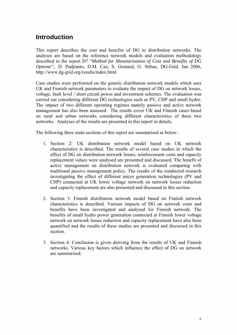
It is assumed that all demand customers are connected at 0.4kV and is composed of 70% of residential customers without electrical heating, 10% of residential customers with electrical heating, 10% of commercial customers and 10% of industrial customers. The annual total load has a maximum of 225MW, a load factor of 0.55, and a power factor of 0.98. Figure 1-1 below shows typical annual load profiles in nine characteristic days used in the studies. Hourly and seasonal load variations were captured and used for load flow analysis. This figure is obtained by aggregating different type of loads, i.e. residential, industrial and commercial loads in the network. Distribution of the loads along feeders was also modelled.

Figure 1-1 Annual load profiles

1.3 Percentage of lines and substations to be upgraded in rural networks

Figure 1-2 to Figure 1-4 present the percentage of 11kV and 33kV lines and 33/11kV substations that need to be upgraded for the different penetration scenarios of DG and for both types of management philosophy: “fit and forget” (F&F) and active management (AM). The case of 2.5GW penetration is not presented since none of the penetration scenarios of DG triggers any reinforcement costs.

For capacities of 5GW and 7.5GW of DG installed over 50% of the GSPs in the UK, less lines require upgrade when DGs are allocated along 2/3 of the circuits than over 1/3 of the circuits, because the capacity of DG installed per line in the first case is low enough to not require reinforcement, whereas when the concentration increases a larger number of reinforcements are required.

On the other hand, as the installed capacity of DG increases to 10GW in the UK, it is the opposite case. The capacity of DG installed per line is such that most of the lines where DG is installed require an upgrade, whatever the penetration density of DG. The higher the density of DG as in scenario H, the lower the number of 11kV lines which need to be upgraded. For the same reasons, when DG is installed over 50% of the GSPs, the number of lines to be reinforced for any penetration of DG is higher for high-density allocation of DG.

Similar comments can be made for 33/11kV substations and 33kV lines: for high

0

50

100

150

200

250

1 2 3 4 5 6 7 8 9 10 11 12 13 14 15 16 17 18 19 20 21 22 23 24

Time

MW

Loa

d

Winter days

Winter Saturday

Winter SundayAutumn/Spring days

Autumn/Spring days

Autumn/Spring SundaySummer days

Summer Saturday

Summer Sunday

12

penetration of DG, the higher the generators concentration in the GSP network, the lower the number of equipment to upgrade. However, the capacity upgrade required is higher for high density of DG and the costs associated are higher, as will be shown in the next sub-section.

0

1

2

3

4

5

6

L (F&F) L (AM) LM (F&F)

LM (AM)

HM (F&F)

HM (AM)

H (F&F) H (AM)

Penetration scenario (Management policy)

Perc

enta

ge o

f sch

eme

to b

e re

plac

ed (%

)

11kV lines 33/11kV transformers 33kV lines Figure 1-2 Percentage of lines and substations to be upgraded in the UK for a DG

penetration of 5GW and for different penetration scenarios

0

1

2 3

4

5

6 7

8

9


LM (AM)

HM (F&F)

HM (AM)

H (F&F) H (AM)


Perc

enta

ge o

f sch

eme

to b

e re

plac

ed (%

)


penetration of 7.5GW and for different penetration scenarios

13

0

2

4

6

8 10

12

14

16

18

L (F&F) L (AM) LM(F&F)

LM(AM)

HM(F&F)

HM(AM)

H (F&F) H (AM)


Perc

enta

ge o

f sch

eme

to b

e re

plac

ed (%

)


penetration of 10GW and for different penetration scenarios

The results obtained with this study also indicate that reinforcement of 11kV lines is driven by voltage constraints as 11kV feeders are characterised by long overhead lines, while the reinforcement of 33/11kV substations and 33kV lines is driven by thermal constraints. As described in the figures above, active management has a positive impact on the percentage of 11kV lines that need upgrading.

1.4 Upgrade cost in rural networks

Figure 1-5 to Figure 1-7 illustrate the total UK upgrade capital costs disaggregated per voltage level and per scenario, and for both passive and active management. They reveal that upgrading 11kV lines is the main cost for all scenarios of penetration of DG. Nevertheless, the cost of upgrading 33/11kV substations increases with the capacity and the density of penetration of DG, and forms a large part of the reinforcement cost in scenario H, and for a penetration of 10GW. These figures also demonstrate how the upgrade costs can be reduced by using active management in 11kV modules. Since the unit cost of various assets is different, it is possible that the upgrade cost for different cases are different although the percentage of circuits to be upgraded in the associated cases are the same as presented in Figure 1-2-Figure 1-4. It can be concluded that if passive approach remains to be used, it will drive more capital investment and increase the cost for integrating DG.

14

0 20 40 60 80

100 120 140 160 180 200


LM(AM)

HM (F&F)

HM(AM)

H (F&F) H (AM)


Upg

rade

cos

t (M

£)

11kV lines 33/11kV transformers 33kV lines Figure 1-5 Upgrade costs for a DG penetration of 5GW

0

50

100

150

200

250

300


LM(AM)

HM (F&F)

HM(AM)

H (F&F)

H (AM)


Upg

rade

cos

t (M

£)

11kV lines 33/11kV transformers 33kV lines

Figure 1-6 Upgrade costs for a DG penetration of 7.5GW

15

0 50

100 150 200 250 300 350 400 450


LM(AM)

HM (F&F)

HM(AM)

H (F&F)

H (AM)


Upg

rade

cos

t (M

£)

11kV lines 33/11kV transformers 33kV lines Figure 1-7 Upgrade costs for a DG penetration of 10GW

In order to determine the operation and maintenance (O&M) cost, 1.4% is applied as the standard annual O&M rate at extra high voltage levels (United Utilities, 2005). This value is assumed for assets at each voltage level for UK distribution networks. Using 7% rate of return and 20 years capital investment time scale, Table 1-6 shows the annuatised upgrade costs and O&M costs for UK rural networks with various DG penetration levels and management policies considering intermittent (I) and non-intermittent (NI) cases.

Table 1-6 Annuatised reinforcement cost and O&M cost in UK rural network

(M£ /year) L LM HM H DG

capacity

Cost type PM AM

NI AM

I PM AM NI

AM I PM AM

NI AM

I PM AM NI

AM I

2.5 GW

Reinf O&M

0 0

0 0

0 0

0 0

0 0

0 0

0 0

0 0

0 0

0 0

0 0

0 0

5GW Reinf O&M

0 0

0 0

0 0

11.89 0.17

0 0

0 0

11.89 0.17

0 0

0 0

22.47 0.31

9.06 0.13

7.93 0.11

7.5 GW

Reinf O&M

9.44 0.13

0 0

0 0

27.85 0.39

4.63 0.06

4.06 0.06

27.47 0.38

4.53 0.06

3.96 0.06

33.89 0.47

25.49 0.36

23.88 0.33

10 GW

Reinf O&M

22.94 0.32

0 0

0 0

45.5 0.64

18.12 0.25

15.95 0.22

44.18 0.62

16.99 0.24

15.01 0.21

53.05 0.74

37.19 0.52

35.49 0.50

1.5 Costs associated with active management

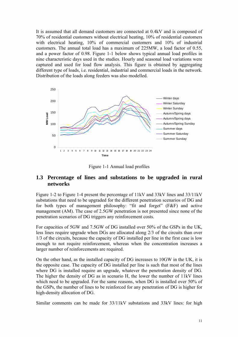
1.5.1 Curtailment cost The first cost associated with active management is the cost of curtailing output of distributed generator, in order not to violate voltage or thermal constraints in times of low demand. This cost can be associated to the opportunity lost of DG due to network constraints. Figure 1-8 shows the energy curtailed for each scenario of non-intermittent DG penetration. The cost associated is obtained by multiplying the amount of energy curtailed by the cost of electricity, which is assumed to be 20£/MWh in this study.

16

0

20

40

60

80

100

120

140

160

180

200

2.5 5 7.5 10DG penetration (GW )

Ene

rgy

cust

aile

d (G

Wh/

year

L LM HM H

Figure 1-8 Energy curtailed for non-intermittent generation

1.5.2 Implementation cost

The second cost associated with active management is its implementation cost. Implementation of generation curtailment necessitates the installation of voltage measurement schemes at the generator point of connection as described in (Liew, S.N., 2002). A reliable communication link between the terminal of the DG and the DSO centre is also required. Besides, in a coordinated area-based voltage control, measurements and communication are also required between a 33/11kV substation and the DSO centre. In this study we suppose that the cost of active management is flat irrespective of the considered level of DG penetration. This is because the cost of active management is assumed for simplicity to be fixed, irrespective of the number of feeders with voltage rise problems as long as there is at least one problem feeder. In rural areas, the cost of implementing active management is therefore supposed to be £10,000 per DG. In urban areas, the cost of implementing active management is assumed £100,000 per substation. However, in practice, the cost of active management has variable cost components and depending on the number of problem feeders, the cost of enabling active management varies.

1.6 Benefits of active management in rural networks

Table 1-7 and Figure 1-9 compare the range of reinforcement and capitalised operation costs for different penetrations of DG in the UK distribution between passive management and active management with all its associated costs described above: energy reduction cost due to curtailment, cost of implementing active management and cost of reinforcement if required. In Table 1-7, the first row in the active management column corresponds to the reinforcement costs for the intermittent case while the second row corresponds to the non-intermittent case. The underlined figures correspond to the cost of implementing active management.

17

Table 1-7 Reinforcement cost (RC) of upgrading feeders and substations in rural system (in M£) for Passive (PM) and Active (AM) management (considering the

intermittent and non-intermittent cases) and cost of implementing (CoI) active management

Scenario ⇒ L LM HM H DG capacity

⇓ PM RC

AM RC CoI

PM RC

AM RC CoI

PM RC

AM RC CoI

PM RC

AM RC CoI

0 0 0 0 2.5GW 0 0 0 0 0 0 0 0 0 0 0 84 5GW 0 0 126 0 80 126 0 80 238 96 40

0 43 42 253 7.5GW 100 0 80 295 49 80 291 48 80 359 270 40

0 169 159 376 10GW 243 0 160 482 192 80 468 180 80 562 394 40

0

200

400

600

800

1000

1200

1400

2.5 5 7.5 10 Installed capacity (GW)

Cos

t (M

£)

Passive rural network Active rural network

Figure 1-9 Ranges of reinforcement cost of upgrade in rural areas

The benefits of active management are clearly illustrated in Figure 1-9 for each penetration of DG. For an installed capacity of 5GW, up to 50% of the cost of upgrading the system could be saved by applying active management, while this figure varies between 15 and 40% for a penetration of 10 GW.

18

Table 1-7 also suggests that reinforcement costs required in the intermittent case are smaller than for the non-intermittent case. This is due to the lower occurrence of the worst-case situation of high output of DG at times of low demand in the intermittent case.

1.7 Benefits of active management in urban networks

In most cases a rise in system fault level requires the switchgear to be replaced with equipment of a higher fault rating. In the developed UK model, the entire switchboard of a substation is replaced if the fault rating at that location is exceeded. The costs of new switchboards used for each voltage level are presented in Table 1-8.

Table 1-8 New switchboard cost Substation GSP 132/33kV 33/11kV

New switchboard cost (£) 3,146,000 1,079,000 497,350

Average system fault levels are assumed at each voltage level; 350MVA at 11kV and 1,000MVA at 33kV, and two different fault level headrooms available at each voltage level are examined. The headroom is used to determine how much DG can be added to various parts of the DSO networks before switchgear fault ratings are exceeded. The two following cases are investigated:

• 0% headroom; in this case the introduction of DG at 11kV requires the upgrade of the switchgear in the 33/11 kV substation.

• 10% headroom; in this case the introduction of DG at 11kV requires the upgrade of the switchgear in the 33/11 kV substation only if its contribution to fault level is superior to 10% of the switchgear rating.

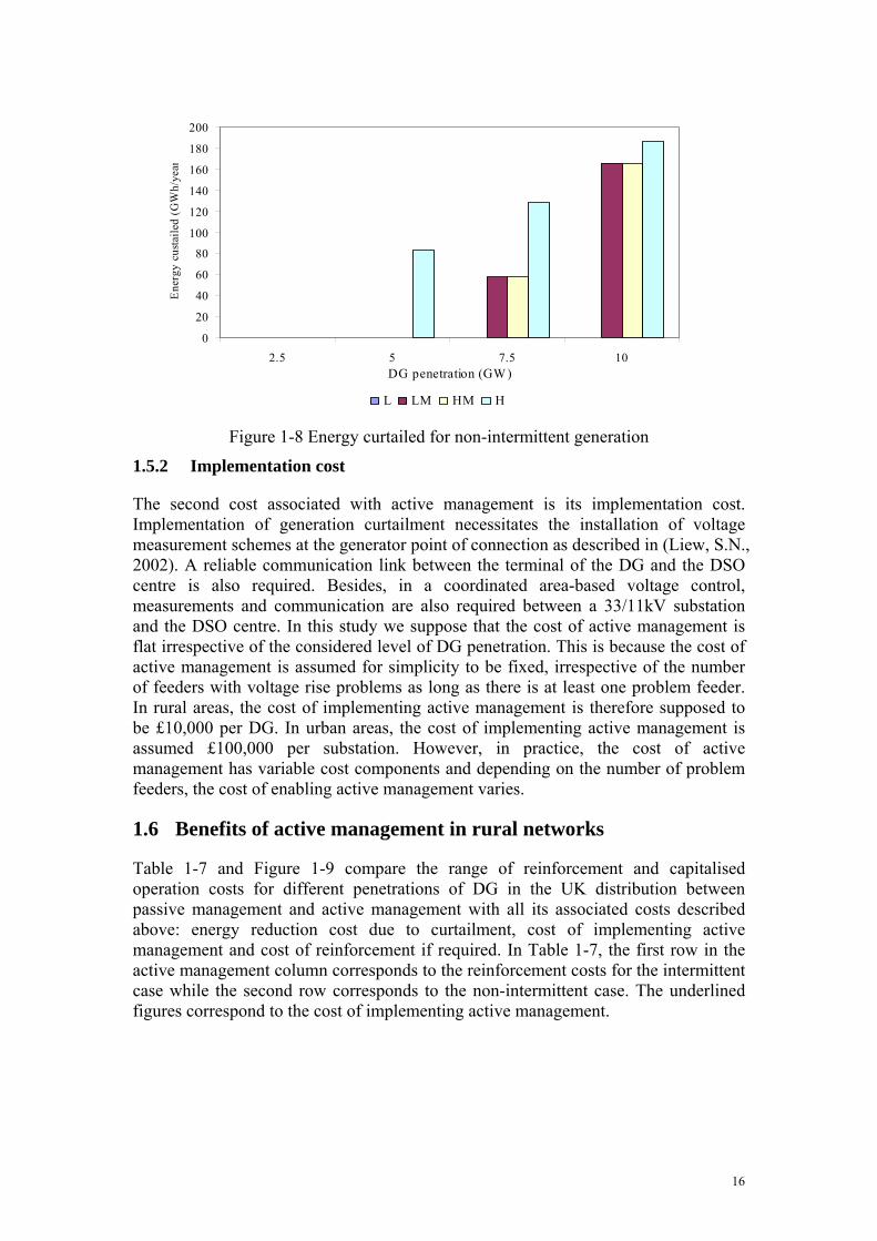
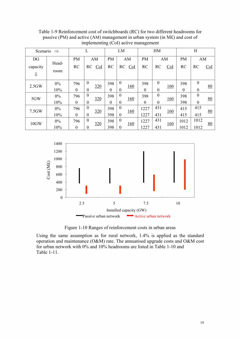
Table 1-9 and Figure 1-10 provide the range of full cost of upgrading switchboards in all the penetration scenarios of DG in urban systems. For active management, the cost of implementing an active managed network is added to the cost of upgrading switchboards. As for rural systems, the benefits of active management can be clearly identified. For low DG penetration, more than half of reinforcement costs could be saved by applying active management.

19

Table 1-9 Reinforcement cost of switchboards (RC) for two different headrooms for passive (PM) and active (AM) management in urban system (in M£) and cost of

implementing (CoI) active management

Scenario ⇒ L LM HM H

DG

capacity

⇓

Head-

room

PM

RC

AM

RC CoI

PM

RC

AM

RC CoI

PM

RC

AM

RC CoI

PM

RC

AM

RC CoI

0% 796 0 398 0 398 0 398 0 2.5GW

10% 0 0 320

0 0 160

0 0 160

0 0 80

0% 796 0 398 0 398 0 398 0 5GW

10% 0 0 320

0 0 160

0 0 160

398 0 80

0% 796 0 398 0 1227 431 415 415 7.5GW

10% 0 0 320

398 0 160

1227 431 160

415 415 80

0% 796 0 398 0 1227 431 1012 1012 10GW

10% 0 0 320

398 0 160

1227 431 160

1012 1012 80

0

200

400

600

800

1000

1200

1400

2.5 5 7.5 10

Installed capacity (GW)

Cos

t (M

£)

Passive urban network Active urban network

Figure 1-10 Ranges of reinforcement costs in urban areas

Using the same assumption as for rural network, 1.4% is applied as the standard operation and maintenance (O&M) rate. The annuatised upgrade costs and O&M cost for urban network with 0% and 10% headrooms are listed in Table 1-10 and Table 1-11.

20

Table 1-10 Annuatised reinforcement cost and O&M cost in urban network with 0% headroom (M£/year)

GW Cost type L(PM) L(AM) LM(PM) LM(AM) HM(PM) HM(AM) H(PM) H(AM)

2.5 Reinf O&M

75.14 1.05

0 0

37.57 0.53

0 0

37.57 0.53

0 0

37.57 0.53

0 0

5 Reinf O&M

75.14 1.05

0 0

37.57 0.53

0 0

37.57 0.53

0 0

37.57 0.53

0 0

7.5 Reinf O&M

75.14 1.05

0 0

37.57 0.53

0 0

115.82 1.62

40.68 0.57

39.17 0.55

39.17 0.55

10 Reinf O&M

75.14 1.05

0 0

37.57 0.53

0 0

115.82 1.62

40.68 0.57

95.53 1.34

95.53 1.34

Table 1-11 Annuatised reinforcement cost and O&M cost in urban network with 10%

headroom (M£/year) GW Cost

type L(PM) L(AM) LM(PM) LM(AM) HM(PM) HM(AM) H(PM) H(AM)

2.5 Reinf O&M

0 0

0 0

0 0

0 0

0 0

0 0

0 0

0 0

5 Reinf O&M

0 0

0 0

0 0

0 0

0 0

0 0

37.57 0.53

0 0

7.5 Reinf O&M

0 0

0 0

37.57 0.53

0 0

115.82 1.62

40.68 0.57

39.17 0.55

39.17 0.55

10 Reinf O&M

0 0

0 0

37.57 0.53

0 0

115.82 1.62

40.68 0.57

95.53 1.34

95.53 1.34

1.8 Effect of DG on distribution losses and distribution network capex

1.8.1 Distribution losses and DG at 11kV Quantifying the variation in annual energy losses due to the introduction of DG with constant output in the UK distribution network is the objective of this section. Due to lacking the number of GSPs for rural and urban networks for the UK, the corresponding results shown below were conducted using average network model, which captures the average characteristics of the UK rural and urban distribution networks, rather than rural and urban network models themselves. And the results are believed to be appropriate enough to show the effect of DG on losses. Since losses at 0.4 kV are not influenced by the connection of DG at 11kV, the different results and figures of this section present the annual energy losses in the entire UK distribution network apart from the low voltage level. The presence of DG at 11kV changes the flow patterns and therefore the losses incurred in transporting electricity through transmission and distribution networks. The first thought is that DG contributes to power loss reduction as the generation energy flow is generally against the major net flow. This is, however, normally but not necessarily true. The impact of DG on losses depends on the penetration and the location of DG in the network as described in Figure 1-11 to Figure 1-14. Low penetration of DG reduces the losses, as the generation is absorbed by local load,

21

which then reduces the flow in the 11kV feeder and in the voltage levels above. However, as the penetration of DG increases, generation starts to exceed local demand, particularly in low loaded lines and at time of low demand, leading to a reverse flow in the 11kV feeders. This reverse flow increases the losses at 11kV and in some cases at higher voltage levels too. Figure 1-11 describes the behaviour of annual energy losses for the penetration scenario where DG is allocated to 2/3 of the 11 kV circuits of 50% of the GSPs in the UK. In that case, for any penetration of DG, the losses in the UK distribution network are lower than when no DG is connected to the network, and a minimum in energy losses is obtained for a DG penetration of 5GW. For low penetration of DG, active management is not required since the system does not need any reinforcement. However for high penetration of DG, the use of active management tends to increase the losses since feeders have smaller sizes than for passive management. For a penetration of 10GW, the corresponding increase in cost of losses is about 3M£/year in the UK network assuming the electricity cost is 20£/MWh.2

0

0.5

1

1.5

2

2.5

3

3.5

0 2.5 5 7.5 10

Penetration of DG (GW)

Loss

es (%

)

Passive management Active management

Figure 1-11 Losses in UK’s distribution network (except for LV) for scenario L Figure 1-12 and Figure 1-13 represent the losses for the penetration scenarios where DG is allocated to 1/3 of the 11 kV circuits of 50% of the GSPs in the UK and DG is allocated to 2/3 of the 11 kV circuits of 25% of the GSPs in the UK respectively. The comments are generally similar to before: the losses for low penetrations of DG (2.5GW and 5GW) are smaller than if no DG is connected to the network. However, as the penetration increases the losses tend to increase in the UK distribution network. Moreover, the losses in these two cases are higher than in the case with a less dense penetration of DG. Similarly to the previous case, active management has a negative impact on losses: energy losses increase by about 15% in the case of high penetration of DG when active management is applied. However the corresponding increases in cost of losses (about 15M£/year for a penetration of 10GW in scenario HM) do not question the benefits of applying active management.

2 Cost of losses is calculated from the annual energy losses multiplied by the specified energy cost.

22

0 0.5

1 1.5

2 2.5

3 3.5

4 4.5

5

0 2.5 5 7.5 10 Penetration of DG (GW)

Loss

es (%

)

Passive management Active management

Figure 1-12 Losses in UK’s distribution network (except for LV) for scenario LM

0

1

2

3

4

5

6


Loss

es (%

)

Passive management Active management Figure 1-13 Losses in UK’s distribution network (except for LV) for scenario HM

Figure 1-14 depicts the losses for the penetration scenario where DG is allocated to 1/3 of the 11 kV circuits of 25% of the GSPs in the UK, which corresponds to a high-density penetration. In this scenario, any penetration of DG increases the losses in the network. This rise can reach 100% when 10GW of DG is connected to the network.

23

0 1 2 3 4 5 6 7 8 9

10


Loss

es (%

)

Passive management Active management Figure 1-14 Losses in UK’s distribution network (except for LV) for scenario H

1.8.2 Distribution network capex and DG Because distributed generators are located near to consumers, the net demand to be supplied from transmission and distribution networks can decrease, postponing the need to reinforce the system in case of load growth or to reduce the investment required in case of equipment replacement. (Mendez, V.H., et al., 2003) assessed the investment deferral in radial distribution networks with distributed generation based on a part of a semi-rural distribution model. However the methodology presented above enables us to study the impact of DG with a flat output on investment deferral in the entire distribution network of the UK for different penetration scenarios (and therefore on security). Table 1-12 presents the maximum flow in the Grid Supply Point of networks where DG is connected. The low-density penetration of DG corresponds to the scenarios L and LM presented above while the high density corresponds to the scenarios HM and H. The maximum flow when no DG is connected to the network is 225MVA in the GSP. The DSO could therefore benefit in the case of a low-density penetration of DG, as the capacity required in the GSP is 2×198MVA instead of 2×225MVA. The minimum flow is obtained for a high density penetration of 7.5GW of DG. It is interesting to note that for high and dense penetrations of DG, the maximum flow in GSPs occurs in times of low demand when power is exported from the distribution network to the transmission network. Similarly, the introduction of DG at 11kV in the network changes the flow in the 132/33kV substations. Table 1-13 describes the maximum flow in each 132/33kV substation when DG is introduced at 11kV. When no DG is installed in the network, the maximum flow is 55MVA.

24

Table 1-12 Maximum flow (in MVA) in GSP substations for GSPs with DG

Maximum flow (in MVA) in GSP substations DG scenario

DG penetration

Low density High density

2.5GW 198 172 5GW 172 123

7.5GW 148 95 10GW 122 145

Table 1-13 Maximum flow (in MVA) in 132/33kV substations for GSPs with DG

Maximum flow (in MVA) in 132/33kV substations

DG scenario

DG penetration


2.5GW 49 43 5GW 43 30

7.5GW 36 23 10GW 30 35

Using the figures in Table 1-12 and Table 1-13, one can derive the potential value (in £M) of DG in replacing distribution network assets in the entire UK. These potential benefits are presented in Table 1-14 in capitalised value.

Table 1-14 Potential value of DG in replacing distribution network assets (£M)

Replacement value of DG (£M) DG scenario

DG penetration


2.5GW 186.24 190.12 5GW 380.24 386.06

7.5GW 582.00 500.52 10GW 776.00 304.58

For low densities of DG penetration at 11kV, the benefits obtained in asset replacement cost increase with the penetration of DG. However the high density scenario, combined with very high penetration of DG tends to decrease these benefits since a high capacity is required at the substations for the upward transfer of power from the 11kV voltage level to the transmission network in times of low demand.

25

1.9 Reduction of losses and provision of network capacity from micro generation

The Engineering Recommendation G83/1 (ER G.83/1, 2003) defines the capacity constraints recommendations for the connection of small scale embedded generators in parallel with public low-voltage distribution networks up to 16A per phase, equating 3.68kVA for a 230V single phase connection. Electricity from micro-generation is both produced and consumed on the premises by technologies such as micro wind, micro hydro, fuel cells, photovoltaics (PV) or micro combined heat and power (micro CHP). In this research only micro CHP and photovoltaics were studied because typical daily and seasonal energy outputs can be used for these two technologies. In the working paper (Distributed Generation Coordination Group, 2004) the different economic benefits delivered by micro generation are summarised as follows:

• It will reduce emissions of COx, SOx, NOx and particulates • It will reduce the total capacity needed within networks • It will reduce the need for peak provision in electricity networks • It will reduce power system losses • It will deliver major energy efficiency gains • It will reduce the amount of large-scale centralised generating capacity

The results presented below quantify the reduction of distribution energy losses and the reduction in total capacity needed for different penetration scenarios of micro CHP and PV in the UK distribution network. Therefore cases studies with 2.5%/5%/7.5%/10% of all UK customers with micro generation over 20%/50% of GSPs in the UK are displayed.

1.9.1 Micro CHP Combined Heat and Power (CHP) is the simultaneous production of electrical power and useful heat. In the case the electrical power of domestic micro CHP is consumed inside the host premises although any surplus or deficit is exchanged with the utility distribution system. The heat generated by micro CHP is used for space heating inside the host premises. Therefore the electrical energy output of micro CHP is driven by the heat requirements of consumers. Figure 1-15 illustrates the normalised generation profile of micro CHP used in this study where it was assumed the output of micro CHP is nil during the summer. Furthermore, it was assumed that 25% of the customers with micro CHP had a technology with a capacity of 3kW and 75% with a capacity of 1.1kW.

26

0

0.2

0.4

0.6

0.8

1

1.2

0 5 10 15 20 Time (Hr)

Mic

ro C

HP

elec

tric

gene

ratio

n (p

u)

Figure 1-15 Normalised output of micro CHP

Table 1-15 gives the annual energy losses and the maximum flow entering in the distribution network for different proportion of customers with micro CHP allocated to 50% of the GSPs in the UK, while Table 1-16 gives the same features when micro CHP is allocated amongst only 20% of the GSPs in the UK. The increase in the proportion of customers with micro CHP leads to a significant reduction in energy losses (from 6.1% to 4.39% in the average network). This reduction is important because the maximum output of micro CHP occurs at time of high customers demand decreasing the transfer of power in the distribution network in times of high demand. For the same reasons the maximum flow entering the GSP network decreases as the capacity of micro CHP increases up to a point where the maximum flow entering the network occurs in at a time when no electricity is produced by micro CHP (like in summer for instance). Similarly to the comments made in section 2.8.2, and since micro CHP generation coincides with peaks of demand, adding micro CHP generation capacity at the low voltage end of the power system defers or removes the need for new network capacity and reduce the utilisation of existing network. This leads therefore to benefits to DSOs. Table 1-15 Losses and maximum flow when micro CHP is allocated to 50% of GSPs

in the UK Losses in GSP with generation (%)/Losses in the

entire UK network (%) Proportion of

customers Average network

Rural network Urban network

Maximum flow entering the GSP (in

MVA) 0% 6.1 8.69 4.47 251.3

2.5% 5.6 / 5.85 7.92 4.12 228.7 5% 5.16 / 5.63 7.24 3.8 206.5

7.5% 4.75 / 5.42 6.63 3.52 187.9 10% 4.39 / 5.24 6.09 3.36 187.9

27

Table 1-16 Losses and maximum flow when micro CHP is allocated to 20% of GSPs in the UK

Losses in GSP with generation (%)/Losses in the entire UK network (%)

Proportion of customers

Average network


Maximum flow entering the

GSP (in MVA)

0% 6.1 8.69 4.47 251.3 2.5% 4.93 / 5.86 6.92 3.72 195.4 5% 4.05 / 5.69 5.62 3.15 187.9

7.5% 3.48 / 5.57 4.78 2.78 187.9 10% 3.18 / 5.51 4.35 2.58 187.9

1.9.2 Photovoltaics Photovoltaic generation corresponds to the direct conversion of sunlight to electricity. Interest is now focused on incorporating the photovoltaic modules into buildings and houses. Thus these small PV installations would be connected directly into customers’ circuits and so interface with the low-voltage distribution network. Figure 1-16 describes the normalised energy profile used in this study based on (Jenkins, N., 1995) to model the output of PV. It is assumed that customers would have a module with a capacity of 1kW.

0

0.2

0.4

0.6

0.8

1

1.2

0 5 10 15 20

Time (Hr)

Nor

mal

ised

ele

ctric

gen

erat

ion

of

PV (p

u)

Summer Autumn/Spring Winter

Figure 1-16 Normalised output of PV Similarly to Table 1-15 and Table 1-16 for micro CHP, Table 1-17 and Table 1-18 describe the distribution losses for different penetrations of PV at 0.4kV. The impact of PV on losses and on the provision of network capacity is less significant then the impact of micro CHP. Indeed, PV in the UK produce electric energy in times of low demand (during summer daytime), but not during peak demands such as the evening of winter weekdays. Therefore the maximum flow entering the distribution network is not affected by the installation of PV (251.3MVA in this example), and even if losses decrease with higher penetrations of PV, the reduction is not significant.

28

Table 1-17 Losses and maximum flow when PV is allocated to 50% of GSPs in the UK


Proportion of customers with

PV Average network



MVA) 0% 6.1 8.69 4.47 251.3

2.5% 5.93 / 6 8.39 4.33 251.3 5% 5.74 / 5.92 8.12 4.2 251.3

7.5% 5.57 / 5.83 7.86 4.09 251.3 10% 5.41 / 5.75 7.62 3.98 251.3

Table 1-18 Losses and maximum flow when PV is allocated to 20% of GSPs in the UK


Proportion of customers with

PV Average network



MVA) 0% 6.1 8.69 4.47 251.3

2.5% 5.65 / 6.01 7.98 4.15 251.3 5% 5.26 / 5.93 7.4 3.88 251.3

7.5% 4.95 / 5.87 6.93 3.65 251.3 10% 4.71 / 5.82 6.58 3.5 251.3

1.10 Summary of the effect of DG connections on UK networks

Corresponding to Table 1-7 and Table 1-9, Table 1-19 and Table 1-20 show the incremental cost (£/kW) for network assets reinforcement in rural and urban networks respectively. The second columns in active management case show the incremental implementation cost of active management. In Table 1-19 for rural networks, the first row in active management case is for intermittent case and the second row is for non-intermittent case. In Table 1-20 for urban networks, the first row corresponds to 0% headroom case and the second row corresponds to 10% headroom case. From Table 1-19 and Table 1-20, we can see that for each DG capacity, in the low and medium DG penetration density cases, the incremental cost can be reduced significantly if active network is applied. While with high penetration level, e.g. for 10GW H penetration scenario, the incremental cost is similar or larger in active management comparing with passive management taking into account the implementation cost of active management.

29

Table 1-19 Incremental cost for assets reinforcement with passive (PM) and active (AM) management for various DG penetration scenarios for rural networks (£/kW)

Scenario ⇒

L LM HM H

DG capacity

PM AM PM AM PM AM PM AM

⇓ IC IC CoI IC IC CoI IC IC CoI IC IC CoI 0 0 0 0 2.5GW 0 0

0 0

0 0

0 0

0 0 0 0 16.8 5GW 0 0 0

25 0

16 25 0

16 48 19.2

8

0 5.7 5.6 33.7 7.5GW 13.3

0 10.7 39.3

6.5 10.7 39

6.4 10.7 47.9

36 5.3

0 16.9 15.9 37.6 10GW 24.3

0 16 48

19.2 8 47

18 8 56

39.4 4

Table 1-20 Incremental cost for assets reinforcement with passive (PM) and active (AM) management for various DG penetration scenarios for urban networks (£/kW)

Scenario ⇒ L LM HM H DG

capacity Head- PM AM PM AM PM AM PM AM

⇓ room IC IC CoI IC IC CoI IC IC CoI IC IC CoI

0% 318.4 0 159.2 0 159 0 159.2 0 2.5GW 10% 0 0

128 0 0

64 0 0

64 0 0

32

0% 159.2 0 79.6 0 79.6 0 79.6 0 5GW 10% 0 0

64 0 0

32 0 0

32 79.6 0

16

0% 106.1 0 53.1 0 164 57.5 55.3 55.3 7.5GW 10% 0 0

42.7 53.1 0

21.3 164 57.5

21.3 55.3 55.3

10.7

0% 79.6 0 39.8 0 123 43.1 101.2 101 10GW 10% 0 0

32 39.8 0

16 123 43.1

16 101.2 101

8

Table 1-21 gives the incremental benefit of DG on network capacity replacement, the value is on average around 76 £/kW for all the cases except the case of 10GW penetration with high density level due to large reversed power flow.

Table 1-21 Incremental replacement benefit of DG (£/kW) Incremental replacement value of DG DG scenario

DG penetration Low density High density 2.5GW 74.496 76.048 5GW 76.048 77.212

7.5GW 77.6 66.736 10GW 77.6 30.458

Incremental value of Micro-CHP on network capacity replacement is shown as Table 1-22. The value is from 23.81£/kW to 83.60£/kW. Since the reason mentioned in

30

section 2.9.2, the maximum power flow does not change with PV installation to the network for each scenario. The incremental value of PV on network capacity replacement is zero and the table is ignored here.

Table 1-22 Incremental benefit of Micro-CHP on replacing distribution network assets (£/kW)

Incremental benefit (£/kW) Proportion of

customers Generator allocated to 50% of GSPs

Generator allocated to 20% of GSPs

2.5% 78.94 83.60 5% 82.83 47.62

7.5% 79.36 31.74 10% 59.52 23.81

31

2 Effect of DG connections on Finnish distribution network

2.1 Finnish generic distribution network models

In order to estimate the costs and benefits of DG connections to Finnish distribution grid, a number of analysis have been conducted for various DG penetration and concentration levels. Studies were performed on generic one-GSP distribution network models. These generic models use several typical circuit parameters, e.g. conductor sizes, lengths, impedances, costs etc. In developing the generic models, different characteristics of networks for different voltage levels and for different network types (rural and urban) are considered, in which the parameters of the networks are obtained from VTT (Technical Research Centre of Finland). Finnish distribution networks comprise three operating voltage levels: 110kV, 20kV and 0.4kV. In developing the generic network models, 110kV networks are excluded from the model for simplicity. Focus of the studies was on the 20 kV and 0.4 kV networks where a number of technical issues will arise with high DG penetrations. It is envisaged that less effect of technical issues DG will bring to the 110 kV networks. Finnish distribution networks are a mix of urban and rural type networks including both short 20 kV feeders in city areas and long overhead line feeders in surrounding areas. In deriving the parameters for the generic models, the Southern Finland is considered as urban area and the rest of Finland as rural. In total, there are 32 GSPs for rural and 14 GSPs for urban networks respectively. In the next sections, models for 0.4kV and 20kV networks are described in more details.

2.1.1 0.4kV network model There are six typical 0.4kV network models in a rural GSP network and five 0.4 kV models in an urban GSP network. A single transformer is installed in each 20kV/0.4kV substation. The total number of transformers installed and their capacity used in our models are listed in Table 2-1.

Table 2-1 Models for 20/0.4kV rural and urban substations Number × capacity of transformers Network

area Model 1 Model 2 Model 3 Model 4 Model 5 Model 6

Rural 200 x 16kVA

640 x 30kVA

960 x 50kVA

640 x 100kVA

640 x 160kVA

120 x 315kVA

Urban 35 x 300kVA

180 x 500kVA

110 x 630kVA

150 x 800kVA

120 x 1MVA

In total there are 10,040 0.4kV circuits included for the rural model and all of them are Aerial Cables (AC) lines with an average length of 0.5km for each circuit. For the urban network model, there are 3135 circuits with an average length of 0.3km for each circuit, among which 2885 circuits are underground (UG) cables and the rest are AC lines.

32

In the studies, a number of different conductor types and sizes are available to be used in the model specifically if 0.4 kV circuits need to be reinforced during the studies. The size and impedance of various circuits considered in the model are listed below:

Table 2-2 Parameters of 0.4kV circuits for 0.4kV rural and urban network models Network

area Cross section

(mm2) R(Ω/km) X(Ω/km) Type

16 2.060 0.090 AC 35 0.938 0.104 AC 50 0.693 0.101 AC 70 0.479 0.097 AC

Rural

120 0.273 0.092 AC 70 0.479 0.097 AC 185 0.182 0.082 UG Urban 240 0.135 0.135 UG

2.1.2 20kV network models

We use one 110kV/20kV substation model for rural networks and two for urban networks. The number and capacity of transformers installed in the substations are listed in Table 2-3. Note that there are two parallel transformers in each urban substation while only a single transformer in each rural 110kV/20kV substation.

Table 2-3 Models for 110/20kV rural and urban substations Number × capacity of transformers Network area Model 1 Model 2

Rural 20 x 20MVA Urban 6 x 2 x 31.5MVA 6 x 2 x 40MVA

In total there are 100 and 108 20kV circuits for rural and urban network models respectively. In the generic rural network model the circuit length ranges from 15km to 70km and in urban network model all the circuits are 5km in length. In the studies, a number of different conductor sizes are available to be used in the model specifically if 20 kV circuits need to be reinforced during the studies. The size and impedance of various circuits considered in the model are summarised in Table 2-4, where OH and UG for circuit type stand for over head and underground respectively.

33

Table 2-4 Parameters of 20kV circuits for rural and urban networks

Network area Cross section (mm2) R(Ω/km) X(Ω/km) Type

34/6 0.847 0.383 OH 54/9 0.535 0.368 OH 85/14 0.337 0.354 OH 132 0.218 0.344 OH

Rural

PAS 70 0.493 0.533 OH 54/9 0.535 0.368 OH 85/14 0.337 0.354 OH 185 0.169 0.119 UG Urban

240 0.130 0.116 UG

2.1.3 Load profiles On the generic network models, loads were populated using a number of characteristic day profiles. There are four types of demand customers considered in the models with different load profiles. They are residential load without electrical heating profile, residential load with electrical heating, commercial load and industrial load. In order to capture hourly temporal variation of loads in different seasons, the characteristic day load profiles for each demand customer type were derived in terms of summer, spring/autumn, and winter business and non business days with hourly time resolution. For rural networks, the load profiles also include a load profile for agriculture customers. In these studies, the 0.4kV peak load in one rural GSP network is 95MW and 10MW for 20kV taking into account the diversity of various load types. The 0.4 kV peak load are 140MW and 80MW for 20kV in an urban GSP network. Figure 2-1 and Figure 2-2 show the characteristic day load profiles used in the studies for rural and urban networks. The profiles are obtained by aggregating the value of various load types at each hour. With different load distribution among different customer types, it is expected that the load profiles for rural and urban networks are different.

34

0

20

40

60

80

100

120

1 3 5 7 9 11 13 15 17 19 21 23

Time (hour)

Load

MW

winter weekdays

Winter Saturdays

Winter Sundays

Spring/Autumn weekdays

Spring/Autumn Saturdays

Spring/Autumn Sundays

Summer weekdays

Summer Saturdays

Summer Sundays

Figure 2-1 Load profiles for a rural GSP network

0

50

100

150

200

250

1 3 5 7 9 11 13 15 17 19 21 23

Time (hour)

Load

MW

winter weekdays

Winter Saturdays

Winter Sundays

Spring/Autumn weekdays

Spring/Autumn Saturdays

Spring/Autumn Sundays

Summer weekdays

Summer Saturdays

Summer Sundays

Figure 2-2 Load profiles for an urban GSP network

2.1.4 DG data A number of DG penetration levels with various allocations across distribution networks were developed. A number of forecasted DG installed capacity for Finland has been provided by VTT. More detailed description can be found in the next sections.

2.2 Description of case studies

2.2.1 DG penetration levels There is no specific target value for DG in Finland (Skytte, K. 2005). At present there are around 800MW DGs primarily connected at 20kV networks and only a small proportion of them are connected at 0.4 kV. Case 1 represents a very similar condition with the present situation where the total installed DG capacity at 20kV and 0.4kV networks is around 800 MW and distributed across rural and urban almost equally. Considering the growth of DG in the future will be higher in rural networks than that in urban networks, other three DG penetration scenarios namely Case 2, 3 and 4 for rural and urban networks

35

respectively were determined. All the four cases are summarised in Table 2-5. The last row in Table 2-5 illustrates the ratio between DG penetration and the network peak load considering the peak load for customers connected to 20 kV and 0.4 kV is around 6.5GW3.

Table 2-5 Total DG installed capacity for rural and urban networks Network area DG installed capacity(MW)

Case 1 Case 2 Case 3 Case 4 Rural 445 490 580 670 Urban 422.5 445 490 535

DG/peak load 13.5% 14.5% 16.6% 18.7%

2.2.2 Allocation of DG

In these studies, we assume all the proposed DGs are medium size DGs and they are connected at 20kV networks. In order to investigate the impact of different distribution of DG in the networks, four different allocation scenarios named as L, LM, HM, and H proposed in section 2 were applied for all levels of DG installed capacity listed in Table 2-5. It can be expected that when DG is more concentrated into a smaller number of feeders, their impact on the power flows at those feeders will be more significant. The allocation of DG for each scenario are summarised in Table 2-6. It should be noticed that the effect of DG in one GSP network will depend on the distribution of DG across the network.

Table 2-6 DG allocation scenarios

DG connected over scenarios

Number of GSPs which have DG out of

total 32 rural GSPs

Number of 20kV feeders which have DG out of total 100 feeders in one GSP

H 8 30 HM 8 70 LM 16 30 Rural

L 16 70

DG connected over scenarios

Number of GSPs which have DG out of total 14 urban GSPs)

Number of 20kV feeders which have DG out of total 108 feeders in one GSP

H 4 36 HM 4 72 LM 7 36 Urban

L 7 72

3 Source: VTT

36

2.2.3 Application of suitable network models for addressing different issues The installation of relatively high DG capacity to distribution networks may trigger a number of technical problems such as voltage rise issues, inadequacy of thermal capacity and the increase in fault level. In order to alleviate network problems, network reinforcement becomes necessary. The reinforcement will incur some costs that need to be minimised. For voltage rise problem, the studies were conducted only using a rural GSP network model since the problem mainly occurs in weak rural networks characterised by long 20kV overhead circuits with small diameters. And for investigating network reinforcement issue due to fault level increase the studies used the urban GSP network model.

2.2.4 Operation philosophies used in the studies In order to assess the benefits and costs of implementing passive and active network management philosophies to facilitate DG connections, these two different philosophies were applied in the studies.

2.2.5 Modelling of intermittent and non intermittent DG Assessment of the impact of intermittent (I) and non-intermittent (NI) DG was proposed for rural network reinforcement studies. Flat output profile was assumed for non intermittent/intermittent DG running with unity power factor. The energy output from intermittent case was assumed to be equal to one third of energy output from non intermittent case.

2.2.6 Benefits and costs of DG connections On one hand, connection of DG may bring a number of benefits in distribution networks such as reduction on distribution losses, deferral of distribution network reinforcement, voltage support, improvement of system security etc. However, quantifying the tangible benefits is a complex task and requires a number of simulations. Scope of our studies in this project is to quantify the benefits of DG connections on the reduction of distribution losses and the deferral of distribution network reinforcement. On the other hand, connection of DG may also incur additional costs due to network capacity reinforcement, new investment in control and communication equipments to enable active network management and increases in distribution system losses especially when DG output increases flows etc. The costs can be quantified by identifying and calculating the cost of upgrading network assets required to facilitate DG connections while maintaining security and operating constraints in distribution systems. The following sections will describe the results for studies conducted on the Finnish generic network models.

37

2.3 Benefits of active management

In these studies, the costs and benefits of implementing passive and active network management to facilitate DG connections according to aforementioned scenarios are quantified. The studies were performed on the urban and rural generic network models. The benefits of active management were derived from the saving obtained in the capital investment with reference to the costs when passive networks were applied. While the cost of active and passive management is quantified by determining the cost of reinforcing assets which need to be updated to support load or DG connections. For active management, the cost of control and communication infrastructure is also added.

2.3.1 Studies on the generic rural network

Network reinforcement for solving voltage rise problems

Results of case studies performed on the generic rural network for quantifying the benefits of active management in solving voltage rise problems due to DG connections are described in this section. Figure 2-3 and Figure 2-4 illustrate the percentage of 20kV feeders that need to be reinforced to curb the voltage rise effect of DG connections for different DG penetration scenarios with passive (PM) and active network management (AM) philosophies. In Finland, the range of statutory voltage change limit is ±5% for 20 kV networks (SFS, 2003). Since DG penetration scenario of 445MW and 490MW demonstrate the same impact on updated feeder number, the results in these two scenarios are shown using the same Figure 2-3. And the same situation is for 580MW and 670MW scenarios shown as Figure 2-4. The results presented are for the whole Finnish rural networks. Using passive management, the ratio of circuits that need to be upgraded varies between 0 % and 9%. While using active management, the ratio varies between 0% and 4.5%. There will be no circuit reinforcement required if the DG penetration level is relatively low. The highest requirement for reinforcement occurs when passive management is applied to facilitate the connection of 580MW and 670MW LM DG scenarios. In these two cases, the number of violated feeders is the highest ones comparing with other cases. It is expected that higher DG penetration level triggers more problems and higher reinforcement costs.

38

0

1

2

3

4

5

6

7

PM AMOper at i on Phi l osophy

Perc

enta

ge o

f 20

kV

feed

ers

with

vol

tage

ri

se p

robl

ems

occu

r(%)

L LM HM H Figure 2-3 The percentage of 20kV feeders upgraded to facilitate connection of

445MW/490MW DG in Finnish rural networks

0123456789

10

PM AMOper at i on Phi l osophy

Perc

enta

ge o

f 20

kV

feed

ers

with

vol

tage

ri

se p

robl

ems(

%)

L LM HM H Figure 2-4 The percentage of 20kV feeders upgraded to facilitate connection of

580MW/670MW DG in Finnish rural networks In Figure 2-4, the lowest requirement to reinforce 20kV circuits with passive management occurs at HM scenario. In this case the ratio of 20 kV circuits that need to be reinforced per GSP is similar as the ratio for the LM case, but because DG in HM case is located in smaller number (25%) of rural GSPs compared with LM case (50% of rural GSPs), the total number of circuits that need to be reinforced becomes less. The results also demonstrate that active operation regime for example by optimising tap changer positions and/or by curtailing temporarily generation output will be able to reduce the requirement to reinforce circuits due to voltage problems. In Figure 2-3 and Figure 2-4 for AM case, there is no circuit reinforcement required for the first three cases (L, LM and HM). However, if the technical problems raised by DG cannot be solved economically using active management , for example if the DG needs to be constrained off too often, a combined active management approach and circuits reinforcement will be the optimum solution as shown in H scenario. In all cases, it can be concluded that by using active management, the number of circuits that need to be reinforced to solve voltage rise problems can be reduced.

39

Capacity reinforcement cost for rural networks

Reinforcement cost depends on the number of circuits that need to be upgraded to facilitate the DG connections. The cost also depends on the type of circuits required to replace the existing circuits. The reinforcement process takes into account the indivisibility of circuits. This approach is in contrast with the approach which assumes that the size of conductors can be increased continuously; thus the results become more realistic. The results of the studies presented in Figure 2-5 to Figure 2-8 show the total Finnish reinforcement costs for 20kV circuits under both passive and active management and also for the non-intermittent/intermittent generation case. The costs shown in those figures correspond to the number of circuits that need to be replaced mentioned in the previous section. It is shown in Figure 2-5 and Figure 2-6 that in most of the cases, reinforcement cost can be avoided by implementing active network management. Even for high DG concentration (scenario H), significant saving can be achieved if active management is implemented. Figure 2-5 and Figure 2-6 also demonstrate that intermittent DG will drive less capacity than non intermittent DG. Thus in both figures, the reinforcement cost for intermittent DG is always less than the reinforcement cost incurred by non intermittent DG. It is expected that intermittent generation will drive less investment since the worst case condition, i.e. when the high output of DG coincides with low demand conditions, tends to be less frequent.

0

20

40

60

80

100

120

445_L 445_LM 445_HM 445_H

DG penetration scenarios

Rei

nfor

cem

ent C

ost (

M€)

PM AM(Non-Intermittent case) AM(Intermittent case)

Figure 2-5 Reinforcement cost with 445MW DG penetration in rural networks

40

Reinforcement cost for 490MW DG installation

0

20

40

60

80

100

120

490_L 490_LM 490_HM 490_H


Rei

nfor

cem

ent C

ost (

M€)


Figure 2-6 Reinforcement cost with 490MW DG penetration in Finnish rural networks


0

20

40

60

80

100

120

580_L 580_LM 580_HM 580_H


Rei

nfor

cem

ent C

ost (

M€)




0

20

40

60

80

100

120

670_L 670_LM 670_HM 670_H


Rei

nfor

cem

ent C

ost (

M€)



41

Operation and maintenance costs

In order to calculate the annuitised reinforcement cost, it is assumed that the time scale to fully recover the capital investment is approximately 20 years with 7% rate of return. Table 2-7 lists the cost of each rural 20kV circuit reinforcement options4. Table 2-8 summarises the annuatised reinforcement cost and O&M cost. The O&M cost of previous studies is presented in Figure 2-9 to Figure 2-12. Except for the O&M cost for scenario with intermittent DG (I), which is indicated specially, all the values of O&M costs are for case studies associated with non intermittent DG. The O&M cost for case with intermittent DG only occurs for case studies associated with scenario H (except for 445MW case) while for other scenarios, the cost is zero (Table 2-8). Table 2-7 Unit investment cost (capitalised) and O&M cost of 20kV circuits for rural

networks Circuit type Investment cost (€/km) O&M cost(€/km/year) O&M cost / investment cost

34/6 6,216 191 3.07% 54/9 8,316 191 2.30% 85/14 9,906 191 1.93% 132 11,375 191 1.68%

PAS 70 13,970 177 1.27% Table 2-8 Annuatised reinforcement cost and O&M cost for rural networks (M€/year)

L LM HM H DG capacity

Cost type (PM) (AM) (PM) (AM) (PM) (AM) (PM) (AM) (AM/I)

445MW Reinf O&M

0 0

0 0

6.28 1.28

0 0

6.57 1.50

0 0

9.91 1.83

3.14 0.64

0 0

490MW Reinf O&M

0 0

0 0

6.62 1.28

0 0

7.33 1.50

0 0

9.91 1.83

3.14 0.64

1.70 0.41

580MW Reinf O&M

7.91 1.93

0 0

9.63 2.02

3.39 0.83

7.72 1.50

0 0

10.47 2.02

4.82 1.01

2.82 0.64

670MW Reinf O&M

7.91 1.93

0 0

10.23 2.02

5.64 1.29

7.72 1.50

3.96 0.96

10.74 2.02

5.11 1.01

4.65 1.01

4 Source : VTT

42

0

2

4

6

8

10

12

14

L(PM) L(AM) LM(PM) LM(AM) HM(PM) HM(AM) H(PM) H(AM)

DG Penetration level(operation philosophy)

Ann

uatis

ed c

ost(M

€/ye

ar)

Reinforcement cost O&M cost

Figure 2-9 Annuatised reinforcement and O&M cost with 445MW DG installation for Finnish rural networks

0

2

4

6

8

10

12

14

L(PM) L(AM) LM(PM) LM(AM) HM(PM) HM(AM) H(PM) H(AM) H(AM/I)


Ann

uatis

ed c

ost(M

€/ye

ar)


Figure 2-10 Annuatised reinforcement and O&M cost with 490MW DG installation

for Finnish rural networks

43

0

2

4

6

8

10

12

14



Ann

uatis

ed c

ost(M

€/ye

ar)



0

2

4

6

8

10

12

14



Ann

uatis

ed c

ost(M

€/ye

ar)



2.3.2 Studies on the generic urban network

Upgrade of switchgear for accommodating the increased fault level

Results of case studies performed on the generic urban network model for quantifying the benefits of active management in solving fault level problems due to DG connections are described in this section. Several methods of fault level reduction are described in (Wu, X., 2003). Splitting network is the common and cheaper option in practice and was used as the active operation approach for urban network case studies. Average system fault level at 20kV urban network is about 80MVA and it is assumed as the switchboard rating in 110kV/20kV substations. The studies assume that all generator contribution to fault level is five times the rating of the generator.

44

Two different fault level head-rooms were examined:

• 0% headroom: in this case the introduction of DG at 20kV requires the upgrade of the switchgear in the 110/20 kV substation.

• 10% headroom: in this case the introduction of DG at 20kV requires the upgrade of the switchgear in the 110/20 kV substation only if its contribution to fault level is 10% above of the switchgear rating.

Figure 2-13 and Figure 2-14 shows the percentage of switchboards that need to be updated in the whole Finnish urban networks for these two cases: 0% headroom case and 10% headroom case with passive and active management.

0

5

10

15

20

25

30

35

422.5MW(PM) 422.5MW(AM) 445MW(PM/AM) 490MW(PM/AM) 535MW(PM/AM)

DG installed capacity(management policy) with 10% headroom case

Perc

ent o

f sw

itchb

oard

nee

d to

be

rein

forc

ed(%

)

L LM HM H

`

Figure 2-13 Percent of switchboard need to be replaced with various DG penetrations

in Finnish urban networks in 0% headroom case

0

5

10

15

20

25

30

35

422.5MW(PM/AM) 445MW(PM/AM) 490MW(PM/AM) 535MW(PM/AM)

DG installed capacity(management policy) with 0% headroom case

Perc

ent o

f sw

itchb

oard

nee

d to

be

rein

forc

ed(%

)

L LM HM H

Figure 2-14 Percent of switchboard need to be replaced with various DG penetrations

in Finnish urban networks in 10% headroom case

45

Except for the 422.5MW L penetration scenario in 10% headroom case, the number of overloaded switchboard is reduced by applying AM comparing with PM, the number doesn’t change with the same density level of different DG capacity in other cases. This is because in these cases the proposed DG capacity for urban network will trigger all the switchboards overloaded irrespective of penetration scenarios, management policies and headrooms. Since the number of overloaded switchboard and the number GSPs with DG are both the highest among all the scenarios, the maximum percentage value occurs at L scenario. Same changing trend will occur for later reinforcement cost figures for the same reason. Figure 2-15 and Figure 2-16 show the effect of various DG penetration levels on fault level (FL) increment on urban 20kV networks ( there are two types for Finnish 20kV network model which is respectively named model 1 and model 2 – see Table 2-3 ) with two headrooms cases and two different management philosophies. The highest FL increment occurs in 0% headroom case with passive management for each DG penetration scenario. Also the Figures show clearly that active management can reduce FL increase dramatically for any DG penetration scenario in both headroom cases.

0

20

40

60

80

100

120

140

160

422.5

_L

422.5

_LM

422.5

_HM

422.5

_H44

5_L

445_

LM

445_

HM44

5_H

490_

L

490_

LM

490_

HM49

0_H

535_

L

535_

LM

535_

HM53

5_H


Faul

t lev

el in

crem

ent d

ue to

DG

(MV

A)

0% HR (PM) 0% HR (AM) 10% HR (PM) 10% HR (AM)

Figure 2-15 Fault level increment at 20kV networks (model 1) due to DG

46

0

20

40

60

80

100

120

140

160

180

200

422.5

_L

422.5

_LM

422.5

_HM

422.5

_H

445_

L

445_

LM

445_

HM

445_

H49

0_L

490_

LM

490_

HM

490_

H53

5_L

535_

LM

535_

HM

535_

H


Faul

t lev

el in

crem

ent d

ue to

DG

(MVA

)


Figure 2-16 Fault level increment at 20kV networks (model 2) due to DG

Reinforcement cost for urban networks

Average cost for switchboards in 110kV/20kV substation is assumed about €380,000. Figure 2-17 to Figure 2-20 represent the total Finnish reinforcement cost of switchboard with two different headrooms and two operation philosophies for various DG installed capacities. From these figures, we can see the reduction of reinforcement cost is driven by the implementation of AM and the headroom of switchboard rating.

0.0

2.0

4.0

6.0

8.0

10.0

12.0

422.5_L 422.5_LM 422.5_HM 422.5_H


Rei

nfor

cem

ent C

ost (

M€)


Figure 2-17 Reinforcement cost with 422.5MW DG installation for urban networks

47

0.0

2.0

4.0

6.0

8.0

10.0

12.0

445_L 445_LM 445_HM 445_H


Rei

nfor

cem

ent C

ost (

M€)


Figure 2-18 Reinforcement cost with 445MW DG installation for urban networks

0.0

2.0

4.0

6.0

8.0

10.0

12.0

14.0

490_L 490_LM 490_HM 490_H


Rei

nfor

cem

ent C

ost (

M€)


Figure 2-19 Reinforcement cost with 490MW DG installation for Finnish urban networks

0.0

2.0

4.0

6.0

8.0

10.0

12.0

14.0

535_L 535_LM 535_HM 535_H


Rei

nfor

cem

ent C

ost (

M€)


Figure 2-20 Reinforcement cost with 535MW DG installation for Finnish urban networks

O&M cost for switchboard is about €1780/year in urban 110kV/20kV substations. Table 2-9 and Table 2-10 show annuatised reinforcement cost and O&M cost with 0% and 10% headroom cases.

48

Table 2-9 Annuatised reinforcement cost and O&M cost in urban network with 0% headroom (M€/year)

MW L(PM) L(AM) LM(PM) LM(AM) HM(PM) HM(AM) H(PM) H(AM)

422.5 Reinf O&M

0.95 0.10

0.25 0.10

0.95 0.05

0.36 0.05

0.95 0.06

0.34 0.06

0.95 0.03

0.41 0.03

450 Reinf O&M

1.00 0.10

0.27 0.10

1.00 0.05

0.39 0.05

1.00 0.06

0.37 0.06

1.00 0.03

0.43 0.03

490 Reinf O&M

1.10 0.10

0.32 0.10

1.10 0.05

0.44 0.05

1.10 0.06

0.42 0.06

1.10 0.03

0.48 0.03

530 Reinf O&M

1.20 0.10

0.37 0.10

1.20 0.05

0.49 0.05

1.20 0.06

0.47 0.06

1.20 0.03

0.54 0.03

Table 2-10 Annuatised reinforcement and O&M cost in urban network with 10%

headroom (M€/year) MW L(PM) L(AM) LM(PM) LM(AM) HM(PM) HM(AM) H(PM) H(AM)

422.5 Reinf O&M

0.75 0.10

0.05 0.10

0.85 0.05

0.26 0.05

0.83 0.06

0.23 0.06

0.89 0.03

0.35 0.03

450 Reinf O&M

0.80 0.10

0.07 0.10

0.90 0.05

0.29 0.05

0.88 0.06

0.25 0.06

0.94 0.03

0.38 0.03

490 Reinf O&M

0.90 0.10

0.12 0.10

1.00 0.05

0.33 0.05

0.98 0.06

0.30 0.06

1.04 0.03

0.43 0.03

530 Reinf O&M

1.00 0.10

0.17 0.10

1.10 0.05

0.39 0.05

1.09 0.06

0.36 0.06

1.14 0.03

0.48 0.03

2.3.3 Additional cost associated with active management

Curtailment of DG output

On active network, in addition to optimising network voltage control devices such as tap changers and reactive compensators the output of DG can be curtailed in order to reduce the voltage rise effect. This effect particularly occurs when demand is low and DG output is high. However, curtailing DG output incurs some costs which include the cost of losing the opportunity to sell energy among other things. Table 2-11 shows the results of the studies with reference to the energy curtailed for various DG penetration levels and for non-intermittent (NI) and intermittent (I) cases.

Table 2-11 Energy curtailed (GWh/year) for whole rural network

Average energy price at 20kV Finnish rural network is assumed to be €47.7/MWh (Source: VTT). Therefore, the energy revenue losses for generator operators can be

L LM HM H Penetration level

NI I NI I NI I NI I 445 MW 0.00 0.00 0.00 0.00 0.00 0.00 0.48 33.93 490 MW 0.00 0.00 9.59 0.96 0.00 0.00 21.46 30.25 580 MW 0.00 0.00 0.60 13.57 17.20 1.72 25.40 40.37 670 MW 0.00 0.00 0.00 29.35 0.18 14.62 0.34 34.56

49

derived as shown in Figure 2-21 and Figure 2-22 respectively for non intermittent and intermittent cases. In most of these cases, higher energy curtailed is required for studies with intermittent DG compared with the energy curtailed for studies with non-intermittent DG. The reason is that in non-intermittent case, considering energy curtailments limit (0.5% of total output), it is more economic to reinforce and replace a number of circuits with larger conductor sizes rather than curtailing energy to mitigates the voltage rise problems. However, this indicates that the less energy curtailment obtained is at the expense of higher assets investment cost.

0

0.2

0.4

0.6

0.8

1

1.2

1.4

445 490 580 670

DG installed capacity(MW)

Ener

gy re

venu

e lo

ss

beca

use

of c

urta

ilmen

t (M

€)

L LM HM H

Figure 2-21 Energy revenue loss due to curtailment in non-intermittent case

0

0.2

0.4

0.6

0.8

1

1.2

1.4

1.6

1.8

2

2.2

445 490 580 670


Ener

gy re

venu

e lo

ss b

ecau

se

of c

urta

ilmen

t (M

€)

L LM HM H

Figure 2-22 Energy revenue loss due to curtailment in intermittent case

AM implementation cost

Using the assumption as the UK case studies, the cost for implementing active management is supposed to be €14,582.4 per DG scheme for Finnish rural networks and €145,824 per substation for urban networks. Table 2-12 and Table 2-13 represent

50

the capitalised cost of implementing active management in the Finnish rural and urban networks.

Table 2-12 Total capital cost (M€) for AM implementation at Finnish 20kV rural networks

DG penetration level DG scenario 445 MW 490 MW 580 MW 670 MW

L 0.00 0.00 0.00 16.33 LM 7.00 7.00 7.00 7.00 HM 8.17 8.17 8.17 8.17 H 3.50 3.50 3.50 3.50

Table 2-13 Total capital cost for AM implementation at Finnish 20kV urban networks

DG scenario

Total cost for AM implementation(M€)

L 8.17 LM 4.08 HM 4.67 H 2.33

The cost of implementing AM in urban networks in these studies is only influenced by the DG density in the one GSP network model. It is important to note that the cost of implementing AM to address the increased fault level due to DG connections may overwhelm its benefits. This is because AM may not significantly reduce the need of reinforcing networks due to the increase of fault level.

2.3.4 Costs and benefits of active management on Finnish networks Considering the costs associated with active management, we combine them with assets upgrade costs that have been analysed previously to get the total investment cost. The costs obtained from studies with active management are then compared with the reinforcement cost required by a passive network in order to quantify the benefits of active management. Figure 2-23 shows the total investment cost of Finnish rural networks in various penetration scenarios with active and passive management and with non-intermittent and intermittent case. The total investment costs in 445MW, 490MW and 580MW L penetration scenarios are zero and not included in Figure 2-23. This figure can indicate clearly the value of AM in Finnish rural networks. 38% to 90% investment cost can be saved if the operation philosophy is changed from passive to active. The results (Figure 2-23) also demonstrate that intermittent DG will drive less investment.

51

0

2040

60

80

100120

140

445_

LM

445_

HM44

5_H

490_

LM

490_

HM49

0_H

580_

LM

580_

HM58

0_H

670_

L

670_

LM

670_

HM67

0_H


Tota

l cos

t(M€)

PM AM ( NI ) AM ( I ) Figure 2-23 Total investment cost with PM and AM philosophy in Finnish rural

networks

For the case studies on the generic urban network models for 422.5MW and 445MW L DG scenarios and for two different headrooms cases, the total investment costs with AM exceed those under PM philosophy because the reduction in the reinforcement cost is less than the implementation cost of the active management. For other scenarios, implementation of active management has clear benefits with reference to the reduction of total investment cost. This situation is shown in Figure 2-24.

0

2

4

6

8

10

12

14

422.5

_L

422.5

_LM

422.5

_HM

422.5

_H44

5_L

445_

LM

445_

HM44

5_H

490_

L

490_

LM

490_

HM49

0_H

535_

L

535_

LM

535_

HM53

5_H


Tota

l inv

estm

ent c

osts

(M€)

0% HR ( PM) 0% HR ( AM) 10% HR ( PM) 10% HR ( AM)

Figure 2-24 Total investment costs in the studies on the generic urban network with PM and AM and two different headroom cases

In order to perform comparisons that are consistent with UK situation, it is assumed that the whole switchboard will need to be replaced no matter how much the fault level increases above its rating. The reinforcement costs with passive management (PM) and active management (AM) are then changed as shown in Table 2-14. In all the cases except for the 422.5MW L density scenario with 10% headroom (HR), DG connection will trigger fault level increases above switchboard rating in Finnish urban

52

networks. The reinforcement cost strongly depends on the number of models and GSPs which have DG. Due to the AM implementation costs, except in the special case mentioned above where AM leads to reduced reinforcement costs, all other cases indicate that for Finish urban networks modified using the assumption described above, AM will result in more reinforcement costs than PM.

Table 2-14 Switchboard reinforcement cost (M€) 422.5MW 445MW 490MW 535MW Scenarios PM AM PM AM PM AM PM AM

L 21.28 21.28

(18.81 with 10% HR)

21.28 29.45 21.28 29.45 21.28 29.45

LM 10.64 14.72 10.64 14.72 10.64 14.72 10.64 14.72 HM 12.16 16.83 12.16 16.83 12.16 16.83 12.16 16.83 H 6.08 8.41 6.08 8.41 6.08 8.41 6.08 8.41

2.4 Effect of DG on distribution network losses

In this section, the results of case studies on evaluating the impact of DG connections on the generic Finnish distribution networks losses are described. Only 20 kV networks and 0.4 kV network losses will be included in the analyses. The studies are used to demonstrate the impact of intermittent and non intermittent DG and also the impact of different DG penetration levels and density levels on the 20 kV and 0.4 kV distribution system losses. Since the DGs are connected at 20 kV network, the changes in losses are particularly due to the changes in 20 kV network losses. Figure 2-25 to Figure 2-28 show the impact of DG connections for various scenarios on distribution network losses. The results are obtained for the case studies with non intermittent DG. For scenario L with 445MW installed capacity, DG contributes to the less energy flows from transmission and hence reduces distribution losses. However, for a large penetration of DG, the losses increase due to the increase in reverse power flows. These figures as well as the later figures in intermittent case also show that losses in the active network tend to be larger than those in the passive network since circuits in the active network tend to be smaller in size, which consequently leads into higher losses.

53

3.1

3.2

3.3

3.4

3.5

3.6

3.7

3.8

3.9

0 445 490 580 670

DG Installed Capacity(MW)

Loss

es(%

)

PM AM

Figure 2-25 Losses in the rural distribution networks for scenario L (non-intermittent DG)

p

0.0

1.0

2.0

3.0

4.0

5.0

6.0

0 445 490 580 670

DG Installed Capacity (MW)PM AM

Loss

es(%

)

Figure 2-26 Losses in the rural distribution networks for scenario LM (non-

intermittent DG)

0.00.51.01.52.02.53.03.54.04.55.0

0 445 490 580 670


Loss

es(%

)

PM AM

Figure 2-27 Losses in the rural distribution networks for scenario HM (non-intermittent DG)

54

p

0.0

1.0

2.0

3.0

4.0

5.0

6.0

7.0

0 445 490 580 670


Loss

es(%

)

PM AM

Figure 2-28 Losses in the rural distribution networks for scenario H (non-intermittent DG)

Considering intermittent case will abate the effect of DG with higher penetration level on losses increase, it is assumed that losses in intermittent case are 0.9 of losses in non-intermittent case for ‘H’ and ‘LM’ penetration scenarios. Conversely, it will decrease the contribution of DG with lower penetration level on the reduction of losses. We use experimental data 1.1 to multiply losses in non-intermittent case for ‘HM’ and ‘L’ penetration scenarios to get losses value in intermittent case. These factors adjust the losses percentage and hence form the changing tendency with various DG installed capacities in intermittent case shown as Figure 2-29 to Figure 2-32.

3.13.23.33.43.53.63.73.83.94.04.1

0 445 490 580 670


Loss

es(%

)

PM AM

Figure 2-29 Losses in rural distribution network for scenario L (intermittent DG)

55

0.00.51.01.52.02.53.03.54.04.55.0

0 445 490 580 670


Loss

es(%

)

PM AM

Figure 2-30 Losses in rural distribution network for scenario LM (intermittent DG)

0.0

1.0

2.0

3.0

4.0

5.0

6.0

0 445 490 580 670


Loss

es(%

)

PM AM

Figure 2-31 Losses in rural distribution network for scenario HM (intermittent DG)

0.0

1.0

2.0

3.0

4.0

5.0

6.0

0 445 490 580 670


Loss

es(%

)

PM AM

Figure 2-32 Losses in rural distribution network for scenario H (intermittent DG)

Figure 2-33 and Figure 2-34 summarise the Finnish rural network losses due to the penetration of non-intermittent / intermittent DGs for various scenarios applied in the networks with active and passive operation philosophies.

56

0.00.51.01.52.02.53.03.54.04.55.05.5

0 445(NI) 445(I) 490(NI) 490(I) 580(NI) 580(I) 670(NI) 670(I)

DG Installed CapacityMW(Output Cases)

Loss

es(%

)

Without DG L LM HM H

Figure 2-33 Losses in the rural passive distribution networks for non-intermittent/intermittent cases with various DG penetration scenarios

0.0

1.0

2.0

3.0

4.0

5.0

6.0

7.0

0 445(NI) 445(I) 490(NI) 490(I) 580(NI) 580(I) 670(NI) 670(I)

DG Installed CapacityMW(Output Cases)

Loss

es (%

)


Figure 2-34 Losses in the rural active distribution networks for non-intermittent/intermittent cases with various DG penetration scenarios

Figure 2-35 and Figure 2-36 shows the losses in the generic Finnish urban networks in non-intermittent and intermittent case respectively. The results for intermittent case were obtained using the adjusting factor mentioned in rural network case studies. Since splitting networks is realised by opening the circuit breakers located between two lower voltage busbars of transformers, the impedance of system between primary and secondary voltage level will be doubled (Wu, X., 2003). For scenario L, the losses decrease but start to increase with more DG installed and higher allocation density.

57

0

0.5

1

1.5

2

2.5

3

3.5

4

4.5

0 422.5 445 490 535


Lose

s (%

)


Figure 2-35 Urban network losses with various DG penetration scenarios (Non-

Intermittent case)

0

0.5

1

1.5

2

2.5

3

3.5

4

4.5

0 422.5 445 490 535


Loss

es(%

)


Figure 2-36 Urban network losses with various DG penetration scenarios (Intermittent

case)

2.5 Effect of DG on distribution network Capex

Another benefit of DG is to replace the system’s distribution and transmission network capacity because they are located close to demand and energy can be consumed directly in local area. Therefore power flow, which is transporting from transmission system decreases. But this is the case only for certain amount of DG installed to network. With higher DG penetration, power flows may start to reverse and the network capacity may start to be driven by DG rather than by demand customers. Since we ignore 110kV voltage level in Finnish distribution network model, only the maximum power flows in 110kV/20kV substations were investigated.

58

Figure 2-37 illustrates the computed maximum power flows measured at the 110kV/20kV substation for various DG penetration scenarios on the generic Finnish active and passive rural network. Maximum power flows in H density level for all DG capacity scenarios are larger than the flow in the case without DG. In other cases the benefit from DG on network capacity replacement can be realised.

0. 00

2. 00

4. 00

6. 00

8. 00

10. 00

12. 00

14. 00

L LM HM H

Penetration Scenario

Max

imum

pow

er fl

ow (M

VA)

Wi t hout DG445MW( PM)490MW( PM)580MW( PM)670MW( PM)445WM( AM)490WM( AM)580WM( AM)670WM( AM)

Figure 2-37 Maximum power flow in one 110kV/20kV substation which has DG with

various DG penetration scenarios for AM and PM philosophy in rural model Also from the curve we can see maximum power flow for each scenario with active management is smaller than that with passive management but not in a large amount in magnitude because of energy curtailment limits for active management. With above maximum power flow value and unit cost for assets, potential benefit of DG (M€) on replacing distribution network assets (110kV/20kV transformer) are assessed in Table 2-15. Positive values mean the Capex will decrease in the corresponding cases. Negative values in H scenario indicate opposite effect of DG on Capex reduction. For L scenario, the value of DG on assets replacement tends to increase with DG capacity increase. For LM and HM cases, it decreases because the excess of maximum flow in these scenarios over this value of non-DG case in substation becomes bigger in magnitude with DG capacity increase.

Table 2-15 Potential benefit of DG on replacing passive (PM) or active (AM) distribution rural network assets (M€)

Scenarios 445 MW 490 MW 580 MW 670 MW L 6.35 6.95 8.13 9.24

LM 3.41 2.79 1.51 0.25 HM 5.01 4.38 3.13 1.86

PM

H -1.45 -2.05 -3.34 -4.64 Scenarios 445 MW 490 MW 580 MW 670 MW

L 6.35 6.95 8.12 9.22 LM 3.48 2.98 1.67 0.40 HM 5.04 4.44 3.39 2.02

AM

H -1.25 -1.72 -2.98 -4.31

59

Figure 2-38 and Figure 2-39 show maximum flow at different substations (model 1 and model 2) in the generic urban network respectively. Table 2-16 represents the potential benefit of DG on replacing urban network assets.

0

5

10

15

20

25

L LM HM HPenetration Scenario

Max

imum

pow

er fl

ow (M

VA

)

Wi t hout DG422. 5MW445MW490MW535MW

Figure 2-38 Maximum power flow in one 110kV/20kV substation (model 1) which

has DG for urban network

0

5

10

15

20

25

30

35

L LM HM HPenetration Scenario

Max

imum

pow

er fl

ow (M

VA)

Wi t hout DG422. 5 MW450MW490MW535MW

Figure 2-39 Maximum power flow in one 110kV/20kV substation (model 2) which

has DG for urban network

Table 2-16 Potential benefit of DG on replacement of urban network assets (M€) Scenarios 422.5MW 445 MW 490 MW 535 MW

L 4.16 4.37 4.76 5.13 LM 3.52 3.30 2.86 2.39 HM 3.78 3.91 3.97 3.50 H 0.16 -0.07 -0.54 -1.00

The potential benefit of DG on network assets replacement in urban area varies from 0.16M€ to 5.13M€ according to various DG penetration levels except H density level with 445MW to 535MW capacity scenarios, in which DG causes more network capacity requirement than non-DG case,.

60

2.6 Effect of micro or mini generation on Finnish distribution network losses reduction and network capacity replacement

In Finland, several micro or mini generation technologies i.e. small hydro power5, diesel generation, biogas and fuel cells, etc exist. These generators are connected at 0.4 kV networks. In order to quantify the effect of small generation connected at the generic Finnish 0.4kV networks; the studies use the output profile of small hydro power generation since it is widely used in rural areas due to the availability of hydro energy from small rivers. The profile is shown in Figure 2-40. The studies focus on the effect of small hydro plant in rural networks. Currently, the total small hydro power plants in Finland is about 40MW and the growth rate is about 9%/year. The forecasted generation capacity cases used in these studies are shown in Table 2-17. The studies assume that all of these generators are allocated at 50% GSPs for low density (L) scenario and 25% GSPs for high density (H) scenario. The number of GSPs which have DG for both scenarios is presented in Table 2-18.

0

0.2

0.4

0.6

0.8

1

1.2

1 5 9 13 17 21

Time(Hr)

P.U

.

Winter Weekdays

Winter Saturday/Sunday

Spring Weekdays

Spring Saturday/Sunday

Summer Weekdays

Summer Saturday/Sunday

Autum Weekdays

Autum Saturday/Sunday

Figure 2-40 Small hydro power generator normalised output profile

Table 2-17 Small hydro power generator installed capacity cases

DG installed capacity(MW) 60 86.25 172.5 210

Table 2-18 Penetration scenarios

5 In this context for Finnish case studies, the capacity of small hydro power is less than 1MW

Scenario Number of GSPs with small generation ( Total 32)

L 16 H 8

61

Table 2-19 Losses and maximum flow when small hydro power generation connected at Finnish rural lower voltage network

Small hydro power generation penetration

scenarios

Losses in the rural networks with DG

(%)

Losses in the whole rural networks (%)

Maximum flow entering

GSP(MVA) without DG 3.42 3.42 111.56 60MW_L 3.29 3.35 109.62 60MW_H 3.16 3.36 107.68

86.25MW_L 3.23 3.33 108.77 86.25MW_H 3.05 3.33 105.99 172.5MW_L 3.05 3.24 105.99 172.5MW_H 2.73 3.25 100.46 210MW_L 2.97 3.20 104.78 210MW_H 2.60 3.22 98.07

Table 2-19 summarises the effect of small hydro power generation on Finnish rural distribution network losses and network capacity replacement. Small hydro power generation connected to Finnish lower voltage rural network decrease the network losses and maximum flow entering GSPs so that bring benefit on network investment deferral or reduction. These effects become clearer with DG penetration levels increase and the minimum losses percent is 2.6% occurring with 210MW H penetration scenario. From Table 2-19 we can see that small hydro generators contribute not only to reduce the maximum flow entering GSP but also to reduce the losses over the distribution network. This is due to the fact that the peak hydro power generation output coincides with peak demand. Comparing with the UK cases, hydro power generation technology has the similar effect on network with that from micro-CHP.

2.7 Summary of the effect of DG connections on Finnish distribution networks

Figure 2-41 and Figure 2-42 represent the incremental investment cost for rural and urban networks considering the assets reinforcement cost as well as all the cost associated with active management for various scenarios. For rural networks, the incremental cost with passive management is from around 122 €/kW to 236 €/kW. For active management, it is from 11.4 €/kW to 81 €/kW for intermittent case and from 14.8 €/kW to around 99.6 €/kW for non-intermittent case. The values are zero for scenario L in all cases except in the case where DG installed capacity is 670MW.

62

0

50

100

150

200

250

445_

LM

445_

HM44

5_H

490_

LM

490_

HM49

0_H

580_

LM

580_

HM58

0_H

670_

L

670_

LM

670_

HM67

0_H


Incr

emen

tal c

ost (

€/kW

)

PM AM(NI) AM(I)

Figure 2-41 Incremental investment cost in active and passive Finnish generic rural networks for various DG penetration scenarios (€/kW)

Figure 2-42 shows the incremental investment cost for various DG penetration scenarios with different headrooms and management philosophies for urban network. The incremental cost ranges from 13.8 €/kW to 25.5 €/kW.

0

5

10

15

20

25

30

422.5

_L

422.5

_LM

422.5

_HM

422.5

_H44

5_L

445_

LM

445_

HM44

5_H

490_

L

490_

LM

490_

HM49

0_H

535_

L

535_

LM

535_

HM53

5_H


Incr

emen

tal i

nves

tmen

t cos

t (€/

kW)


Figure 2-42 Incremental investment cost with various DG penetration scenarios and management philosophies for Finnish urban networks (€/kW)

From Table 2-15 and Table 2-16, we could derive the incremental DG benefit on replacing distribution network assets with passive management and active management for rural and urban networks shown as Table 2-20 and Table 2-21. These DGs are connected at 20kV networks. From these two tables we can see the benefit of DG on network capacity replacement is higher with lower DG penetration levels. Large amount of DG installation will cause opposite effect on network capacity reduction, which is reflected from the negative values.

63

Table 2-20 Incremental benefit of DG on replacement of Rural network assets (€/kW) Scenarios 445 MW 490 MW 580 MW 670 MW

L 14.27 14.19 14.02 13.79 LM 7.67 5.68 2.61 0.37 HM 11.26 8.94 5.40 2.77

PM

H -3.26 -4.19 -5.76 -6.92 Scenarios 445 MW 490 MW 580 MW 670 MW

L 14.27 14.19 14.00 13.76 LM 7.81 6.09 2.87 0.60 HM 11.34 9.07 5.84 3.01

AM

H -2.80 -3.50 -5.14 -6.43

Table 2-21 Incremental benefit of DG on replacement of Urban network assets (€/kW) DG installed capacity (MW) Density

level 422.5 490 580 670 L 9.85 8.91 8.20 7.66

LM 8.34 6.74 4.94 3.57 HM 8.95 7.98 6.84 5.23 H 0.38 -0.14 -0.92 -1.49

Table 2-22 shows the incremental benefit from small hydro power generation on rural network assets replacement. The value is around 15 €/kW for low density level and 31 €/kW for high density level irrespective of generation capacity. Table 2-22 Incremental benefit of small hydro power generation on of Rural network

assets replacement (€/kW) Density level Generation

capacity L H 60MW 15.39 30.75

86.25MW 15.38 30.71 172.5MW 15.35 30.59 210MW 15.35 30.54

64

3 Summary This report describes the cost and benefit of DG on the UK and Finish distribution networks. On one hand, the cost of DG connections is obtained by calculating the cost of network reinforcement needed to mitigate the technical problems, such as voltage rise problems in rural networks and the increase in fault level (short circuit capacity) in urban networks that are caused by its connection. On the other hand, the benefit of DG is determined by computing the reduction in distribution losses and the ability of DG to release network capacity which can be used to accommodate future loads. The studies were carried out using the developed generic networks. Different network characteristics in rural and urban areas and different network control schemes i.e. active and passive control have been modelled and used in these studies to evaluate the impact of different DG penetration levels within the different distribution networks. The impact of different micro generation technologies such as PV, CHP and small hydro on distribution networks was also studied. The drivers which affect the cost and benefit of DG on the system are summarised as below. 1. DG penetration and density level

Greater installed capacity of DG and denser DG penetration will result in more feeders with voltage rise problems in rural networks and will require that more protection assets are updated in urban networks. Hence the reinforcement cost will increase as the DG penetration level increases. DG will contribute in the reduction of system losses when DG reduces power flows across distribution networks. This is likely to happen when the penetration level is relatively low and DG is distributed judiciously in distribution networks. However, the studies have demonstrated increase in losses with high penetration of DG and high density of DG allocation.

2. Network management philosophy (active vs. passive networks) Under the traditional ‘Fit and forget’ approach, i.e. passive network operation philosophy, a large amount of investment is needed to upgrade current network assets. The benefit of active management for reducing these upgrade costs is clear for UK networks and Finnish rural networks. When it is assumed, however, that the entire switchboard must be replaced if required, then in most cases, reinforcement costs for Finish urban networks when using AM are larger than the reinforcement costs with PM. Evaluation of the benefits of AM should consider the AM implementation cost, which covers additional control and communication devices on the networks. Although losses in AM are higher than those in PM due to the continued use of smaller sized assets, the cost of losses is much small in comparison with investment costs. However, the application of active network should not be justified only with the reduction of cost in distribution network but also with its benefits for transmission and the overall system. In the highly distributed power system, controllability of DG facilitated by active network to support transmission and distribution system operation is essential.

3. DG technologies

The effect from non-intermittent and intermittent generation on the distribution network capacity and losses depends on the variability of imbalance between load

65

and generation occurring. Some renewable technology depends on the location of energy source and seasons. CHP has more flexibility in where is can be located than Hydro power generation, so it can have an impact on both rural and urban network. Hydro power is only for rural network. The Micro CHP applied in the UK case and small hydro power applied in the Finnish case both have similar effects on network loss reduction and network capacity replacement because of the coincidence of DG maximum output with peak load. PV has weaker effect in UK since the maximum output of PV occurs in summer while maximum load is in winter.

The results of case studies carried out on the generic UK and Finnish networks can be summarised as follows, in which the results in the unit of sterling pounds for the UK studies are converted into Euro using exchange rate: 1 GBP = 1.5 EUR • Investment cost of distribution networks due to DG integration. Rural networks All the proposed DG is assumed to be connected at medium voltage level circuits. The incremental cost of rural network asset reinforcement is zero for low DG penetration levels in both the UK and Finnish networks. That means the current networks have the ability to accommodation small amount of DG without any reinforcement due to voltage rise problems. Once investment is required, for UK networks with passive management the incremental cost changes from 20€/kW to 83.7€/kW with various DG penetration levels. In networks applying active management with medium and high DG installation, incremental cost changes from 16€/kW to around 64.9€/kW for both intermittent and non-intermittent cases with considering costs associated with active networks operation. The incremental investment costs in medium and high DG penetration scenarios with passive management for Finnish rural networks range from 122€/kW to 236€/kW. With active management, the incremental investment cost drops to 11.4€/kW-81€/kW for intermittent case and 14.8€/kW-99.6/kW for non-intermittent case. The comparison of non-zero incremental cost between UK and Finnish rural networks is listed in Table 3-1.

Table 3-1 Incremental cost comparison between UK and Finnish rural networks

when network assets replacement required (€/kW) UK rural networks Finnish rural networks

Network Management Philosophy

Passive Management

Active Management

Passive Management

Active Management

€/kW 20-83.7 16-64.9 122-236 11.4-99.6

Theses results show that cost of DG penetration strongly depends on the characteristics of the networks. Additionally, the benefit of active management to investment cost saving is higher in Finnish rural networks than the corresponding benefits in the UK. The values in Finnish cases are much larger than those in UK case. This is caused mainly due to following reasons.

66

1. Firstly, the average length of overhead lines which experience problems is around

20km in UK rural networks while this value for Finland is from 30km to 70km which are 1.5 to 3.5 times of UK cases. With the same order of magnitude of unit reinforcement cost per kilometre, circuit replacement will result in more investment costs with longer lines.

2. Secondly, most of the loads in the Finnish network model are located close to the

substation and only a small amount of loads can be used to absorb DG connected at the end of the feeder. In this case, DG connection will trigger voltage rise problems and hence require circuit reinforcement in any scenario. Also, the voltage rise problem is more severe and reinforcement costs are higher compared with the UK cases since in the UK rural network model, the loads are mainly distributed increasingly or uniformly along the feeder.

3. The third reason is due to assumptions in the circuit reinforcement options. For

UK case, we assumed the size of circuit can increase linearly. So we increased the problem circuit size linearly until the voltage problems are resolved so that minimum cost option can be obtained for circuit reinforcement. But for Finnish case, indivisibility of circuit sizes was assumed. This means very big circuits might be needed, with high reinforcement cost, if the second biggest size circuit can not solve voltage rise problem.

Urban networks For urban networks, without any headroom left for accommodating the increase in fault level, DG connections will immediately cause switchboard reinforcement in passive networks. Under these conditions, the incremental cost in UK urban networks varies from 58.9€/kW to 471.5€/kW. With 10% headroom available in the switchgear rating, the incremental cost is in the range of 0 to 243€/kW for the UK. For Finnish urban networks the incremental cost is from 11.4€/kW to 50.4€/kW for both headrooms. With Active management, urban networks incremental reinforcement cost in the UK can be reduced into the range of 23.8€/kW to 189.6€/kW. An exception to this is the ‘L’ density 422.5MW with 10% headroom case. Other cases show for the Finnish network that the cost is bigger with AM than the corresponding value with PM with the value for AM varying from 15.7 €/kW– 69.7€/kW. Table 3-2 gives the range on these values.

Table 3-2 Incremental cost comparison between UK and Finnish urban networks

(€/kW) UK urban networks Finnish urban networks

Management Philosophy

Passive Management

Active Management

Passive Management

Active Management

Head rooms 0% 10% 0% 10% 0% 10% 0% 10%

€/kW 58.9 -471.5

0 - 243

23.8 -189.6

23.8 -189.6

11.4-50.4

11.4-50.4

15.7-69.7

15.7-69.7

From above results, we can see the same unit DG penetration can lead to much more network reinforcement costs in UK urban networks than in Finnish urban networks.

67

This is caused by the network model characteristics as well as the reinforcement cost of switchboard in either network.

The UK generic distribution network model covers 3 voltage levels of 11kV, 33kV and 132kV when considering DG effect on network fault level. Therefore the reinforcement cost on switchboard includes more than one voltage level in large amount of DG penetration case, for example 7.5GW and 10GW of DG in the HM and H scenarios in which the maximum incremental costs occur. Also the cost of switchboards is very high in higher voltage level substations. This can be seen in Table 1-8 for the UK situation. In Finnish case only fault level rise at 20kV voltage level networks is considered and the whole switchboard cost is 380,000€. Apparently more complex networks and more expensive assets contribute to more reinforcement costs. Generally it can be concluded that active management application can reduce reinforcement cost if there is still headroom left.

• Benefits of DG on network losses and capacity reduction. The range of effects of DG connected at medium voltage level on UK and Finland networks are shown in Table 3-3 which focuses on the differences between the value of losses before and after DG connection. Here we introduce the same adjust factors for intermittent case, which is described in section 3.4 for Finnish networks, to UK case studies. The negative value in bracket means losses increase.

Table 3-3 Effect range of DG on UK and Finnish distribution networks losses reduction (average value)

UK Finland Network

Management Philosophy

Passive Management

Active Management

Passive Management

Active Management

Non-intermittent /Intermittent NI I NI I NI I NI I

Losses (%) Reduction

(-4.4) -0.62

(-3.6) -0.6

(-6.2) -0.62

(-5.3) -0.6

(-1.0) -0.04

(-0.88) -0.002

(-1.55) -0.04

(-1.3) -0.002

The Incremental benefit of DG on network capacity replacement costs for the UK case remains around 112.5€/kW except when the value drops to 45.1€/kW in 10GW with ‘H’ density level scenario in which large reversed power flow occurs. This value for Finnish rural networks varies from 0.37€/kW to 14.27€/kW and from 0.38€/kW to 9.85€/kW for urban networks apart from the H density level for which almost all the DG capacity scenarios with negative values occur. In other words, too high DG penetration will not bring benefit of network reinforcement deferral. The incremental benefit on UK network capacity replacement is much bigger than Finnish case. This is because DG connection can bring more contribution to capacity replacement for UK networks because it covers from 11kV to 132kV voltage level networks including more expensive substations. For Finnish case, only 110kV/20kV substations capacity is considered to be replaced. Comparing the values of incremental network investment costs with incremental potential benefits of DG on network capacity replacement, we can see the investment saving due to the network reinforcement deferral can not offset the network upgrading

68

cost for each scenario. Generally higher benefits occur in relatively low DG penetration levels with lower density scenarios. • Benefits of micro or mini generation on network losses and capacity reduction. Because micro (or mini) generation is connected directly at low voltage networks where the most distribution network customers are connected, these generations could contribute effectively in the reduction of network losses. In the UK, on average the losses can be reduced by 0.4 %-0.8% depending on the production profiles of the micro generation. While the benefit of small hydro power generation in Finnish rural networks in term of losses is around 0.2%. The benefit of micro or mini generation on network investment deferral strongly depends on the production profiles of micro generation and load profiles of demand customers. The benefit from PV is zero in the UK. And Micro-CHP incremental benefit is from 35.4£/kW to 124£/kW for UK case. The incremental benefit from small hydro power generation is about 15.36€/kW for L density level and 30.6€/kW for H density level situations. In both cases, micro generation brings positive value to the UK and Finnish network capacity replacement

69

4 References

D. Pudjianto, D.M. Cao, S. Grenard, G. Strbac, “Deliverables D7: Method for Monetarisation of Cost and Benefits of DG Options”, Report for DG-Grid, Jan 2006, http://www.dg-grid.org/results/index.html.

Green, P., Smith, S. and Strbac, G. (1999) “Evaluation of alternative distribution network design policy”, IEE Electric Power Distribution System Engineering, Vol. 146, 53-60.

Jenkins, N., Allan, R.N., Crossley, P., Kirschen, D. and Strbac, G. (2000) “Embedded Generation”, Institution of Electrical Engineers, London.

Liew, S.N. (2002b) “Technical and Economic Assessments of Active Distribution Networks”. PhD thesis. The University of Manchester Institute of Science and Technology.

“Statement of charging methodology for use of united utilities electricity PLC’s electricity distribution network”. United Utilities Electricity PLC. April 2005.

Mendez, V.H., Rivier, J., de la Fuente, J.I., Gomez, T., Arceluz, J. and Marin, J. (2003) “A Monte Carlo approach for assessment of investments deferral in radial distribution networks with distributed generation”, IEEE Power Tech Conference’2003, Bologna, Italy.

Engineering Recommendation (ER) G.83/1, (2003) “Recommendation for the connection of small-scale embedded generators (up to 16A per phase) in parallel with public low-voltage distribution networks”, Energy networks association. http://www.energynetworks.org/spring/engineering/distributedgeneration02.asp

Jenkins, N. (1995) “Photovoltaic systems for small-scale remote power supplies”, Power Engineering Journal.

Skytte, K. and Ropenus, S. (2005) “Regulatory Review and International Comparison of EU-15 Member States”, Report for DG-GRID. http://www.dg-grid.org/results/result_report-skytte1.pdf

“Finnish standards association (SFS)”, 2003. SFS Handbook 142. ISBN 952-5420-08-6.

Wu, X., Mutale, J., Jenkins, N. And Strbac, G. (2003) “An investigation of network splitting for fault level reduction”, Working Paper for Tyndall Center.

Engineering Recommendation (ER) G.59/1, (1991) “Recommendations for the connection of embedded generating plant to the public electricity suppliers’ distribution systems” 1991 The Electricity Association”, Electricity Networks Association.

Engineering Recommendation (ER) G.75, (2002) “Recommendations for the connection of embedded generating plant to public distribution systems above 20kV or with outputs over 5MW”, Electricity Networks Association.

cost/benefits of dg connections to grid system and benefits of dg connections to grid system d.m....

Documents