crabs in cold water regions: biology, management, and economics
TRANSCRIPT
A.J. Paul, Earl G. Dawe, Robert Elner, Glen S. Jamieson,Gordon H. Kruse, Robert S. Otto, Bernard Sainte-Marie,
Thomas C. Shirley, and Douglas Woodby, Editors
Proceedings of the symposium Crab2001, Crabs in ColdWater Regions: Biology, Management, and Economics
January 17-20, 2001, Anchorage, Alaska, USA
University of Alaska Sea Grant College ProgramAK-SG-02-01
Price: $40.00
BIOLOGY, MANAGEMENT, AND ECONOMICS
NAT
ION
AL
OC
EA
NICAND ATMOSPHERIC
ADMIN
IST
RAT
ION
US
DEPARTMENT OF COMMER
CE
University of Alaska Sea GrantP.O. Box 755040205 O’Neill Bldg.Fairbanks, Alaska 99775-5040Toll free (888) 789-0090(907) 474-6707 Fax (907) 474-6285http://www.uaf.edu/seagrant/
Elmer E. Rasmuson Library Cataloging-In-Publication Data
Crabs in cold water regions : biology, management, and economics / Editors: A.J. Paul … [etal.]. Fairbanks, Alaska : University of Alaska Sea Grant, [2002].
876 p. ; cm. – (Lowell Wakefield Fisheries Symposium ; [19th]), (University of AlaskaSea Grant College Program ; AK-SG-02-01)
Note: “... Proceedings of the symposium Crab2001, Crabs in cold water regions:biology, management, and economics, January 17-20, 2001, Anchorage, Alaska, USA.”
Includes bibliographical references and index
1. Crabs—Congresses. 2. Crab fisheries—Congresses. I. Title. II. Paul, A. J. III. Series:Lowell Wakefield Fisheries Symposium series ; 19th. IV. Series: Alaska Sea Grant CollegeProgram report ; AK-SG-02-01.
QL444.M33 C73 2002
ISBN: 1-56612-077-2
Citation for this volume is: 2002. A.J. Paul, E.G. Dawe, R. Elner, G.S. Jamieson, G.H.Kruse, R.S. Otto, B. Sainte-Marie, T.C. Shirley, and D. Woodby (eds.). Crabs in Cold WaterRegions: Biology, Management, and Economics. University of Alaska Sea Grant, AK-SG-02-01, Fairbanks. 876 pp.
CreditsThis book is published by the University of Alaska Sea Grant College Program, which iscooperatively supported by the U.S. Department of Commerce, NOAA National Sea GrantOffice, grant no. NA86RG-0050, project A/161-01; and by University of Alaska Fairbankswith state funds. University of Alaska is an affirmative action/equal opportunity institu-tion.
Sea Grant is a unique partnership with public and private sectors combining re-search, education, and technology transfer for public service. This national network ofuniversities meets changing environmental and economic needs of people in our coastal,ocean, and Great Lakes regions.
iii
Contents
About the Symposium .................................................................................. ix
The Lowell Wakefield Symposium Series ................................................. ix
Proceedings Acknowledgments ................................................................. x
Correct Spelling and Publication Date for the Golden King Crab(Lithodes aequispinus Benedict, 1895)
Thomas C. Shirley ....................................................................................... 1
Checklist of Alaskan CrabsBradley G. Stevens ....................................................................................... 5
Life History, Growth, and MortalitySetal Stage Duration of Female Adult Dungeness Crab(Cancer magister)
Todd W. Miller and David Hankin ................................................................ 9
Estimating Intermolt Duration in Giant Crabs(Pseudocarcinus gigas)
Caleb Gardner, Andrew Jenkinson, and Hendrik Heijnis ........................... 17
Molting of Red King Crab (Paralithodes camtschaticus)Observed by Time-Lapse Video in the Laboratory
Bradley G. Stevens ..................................................................................... 29
Growth of Red King Crabs from theCentral Aleutian Islands, Alaska
Ivan Vining, S. Forrest Blau, and Douglas Pengilly .................................... 39
Estimating Natural Mortality of King Crabs from TagRecapture Data
M.S.M. Siddeek, Leslie J. Watson, S. Forrest Blau,and Holly Moore ........................................................................................ 51
Estimating Molting Probabilities of Female DungenessCrabs (Cancer magister ) in Northern California:A Multi-Stage Latent Variable Approach
Qian-Li Xue and David G. Hankin .............................................................. 77
iv
Contents
Effects of Windchill on the Snow Crab (Chionoecetes opilio)Jonathan J. Warrenchuk and Thomas C. Shirley ....................................... 81
Testing Carapace Morphology Characteristicsfor Field Identification of Chionoecetes Hybrids
Daniel Urban, Douglas Pengilly, Luke Jadamec,and Susan C. Byersdorfer .......................................................................... 97
Life History of the Galatheid Crab Munida subrugosain Subantarctic Waters of the Beagle Channel, Argentina
Federico Tapella, M. Carolina Romero, Gustavo A. Lovrich,and Alejandro Chizzini ........................................................................... 115
The Complete Larval Development of Chionoecetesjaponicus under Laboratory Conditions
Kooichi Konishi, Toshie Matsumoto, and Ryo Tsujimoto ........................... 135
Growth, Maturity, and Mating of Male Southern KingCrab (Lithodes santolla) in the Beagle Channel, Argentina
Gustavo A. Lovrich, Julio H. Vinuesa, and Barry D. Smith ....................... 147
Growth and Molting of Golden King Crabs (Lithodesaequispinus) in the Eastern Aleutian Islands, Alaska
Leslie J. Watson, Douglas Pengilly, and S. Forrest Blau ............................ 169
Larval Culture of the King Crabs Paralithodescamtschaticus and P. brevipes
Jiro Kittaka, Bradley G. Stevens, Shin-ichi Teshima,and Manabu Ishikawa ............................................................................. 189
Injuries and Aerial Exposure to Crabs duringHandling in Bering Sea Fisheries
Donn A. Tracy and Susan C. Byersdorfer ................................................. 211
Reproductive Biology and BehaviorSize at Maturity of Kodiak Area Female Red King Crab
Douglas Pengilly, S. Forrest Blau, and James E. Blackburn ...................... 213
Mating Pairs of Red King Crabs (Paralithodescamtschaticus) in the Kodiak Archipelago, Alaska,1960-1984
Guy C. Powell, Douglas Pengilly, and S. Forrest Blau ............................... 225
v
Contents
Acoustical Behavior in King Crab(Paralithodes camtschaticus)
Larissa K. Tolstoganova ........................................................................... 247
Preliminary Notes on the Reproductive Conditionof Mature Female Snow Crabs (Chionoecetes opilio)from Disko Bay and Sisimiut, West Greenland
AnnDorte Burmeister ............................................................................... 255
The Sperm Plug Is a Reliable Indicator of Mating Successin Female Dungeness Crabs (Cancer magister )
Shauna J. Oh and David G. Hankin ......................................................... 269
Observations on Rearing Red King Crab (Paralithodescamtschaticus) Zoeae and Glaucothoe in a RecyclingWater System
Nikolina Kovatcheva ................................................................................ 273
Reproductive Biology of Lithodes santolla in theSan Jorge Gulf, Argentina
Julio H. Vinuesa and Pamela Balzi ........................................................... 283
Fecundity of Red King Crabs (Paralithodes camtschaticus)off Kodiak Island, Alaska, and an Initial Look atObserver Agreement of Clutch Fullness
B. Alan Johnson, S. Forrest Blau, and Raymond E. Baglin ........................ 305
Reproductive Cycle of the Helmet Crab(Telmessus cheiragonus)
Jiro Nagao and Hiroyuki Munehara ........................................................ 323
Spatiotemporal Trends in Tanner Crab(Chionoecetes bairdi ) Size at Maturity
Robert S. Otto and Douglas Pengilly ........................................................ 339
Recruitment and Population DynamicsA New Method to Estimate Duration of MoltStages in Crustaceans
David Hankin .......................................................................................... 351
Assessment and Management of Crab Stocks underUncertainty of Massive Die-offs and Rapid Changes inSurvey Catchability
Jie Zheng and Gordon H. Kruse ............................................................... 367
vi
Contents
Trends in Prevalence of Bitter Crab Disease Caused byHematodinium sp. in Snow Crab (Chionoecetes opilio)throughout the Newfoundland and LabradorContinental Shelf
Earl G. Dawe ........................................................................................... 385
Bitter Crab Syndrome in Tanner Crab (Chionoecetesbairdi ) Alitak Bay, Kodiak, Alaska 1991-2000
Daniel Urban and Susan C. Byersdorfer .................................................. 401
Reproductive Capacity Morphometrically Assessedin Cancer pagurus from the Shetland Islands
Shelly M.L. Tallack ................................................................................... 405
Studies on Red King Crab (Paralithodes camtschaticus)Introduced to the Barents Sea
Knut E. Jørstad, Eva Farestveit, Hari Rudra,Ann-Lisbeth Agnalt, and Steinar Olsen .................................................... 425
Fisheries and Stock AssessmentA New Fishery for Grooved Tanner Crab (Chionoecetestanneri ) off the Coast of British Columbia, Canada
G.D. Workman, A.C. Phillips, F.E. Scurrah, andJ.A. Boutillier ........................................................................................... 439
Restratification of Red King Crab Stock AssessmentAreas in Southeast Alaska
John E. Clark, Sandy Hinkley, and Timothy Koeneman ........................... 457
Retrospective Length-Based Analysis ofBristol Bay Red King Crabs: Model Evaluationand Management Implications
Jie Zheng and Gordon H. Kruse ............................................................... 475
Population Assessment Using a Length-BasedPopulation Analysis for the Japanese Hair Crab(Erimacrus isenbeckii)
Hiroshi Yamaguchi, Yuji Ueda, Yasuji Kanno, andTakashi Matsuishi .................................................................................... 495
Population Structure of Blue King Crab (Paralithodesplatypus) in the Northwestern Bering Sea
M.V. Pereladov and D.M. Miljutin ............................................................. 511
vii
Contents
Methodological Problems Associated with AssessingCrab Resources Based on Trap Catch Data
Sergey A. Nizyaev and Sergey D. Bukin ................................................... 521
Inquiry for Application of Data Collected by ObserversDeployed in the Eastern Bering Sea Crab Fisheries
Mary Schwenzfeier, Holly Moore, Ryan Burt, andRachel Alinsunurin .................................................................................. 537
Environmental, Ecological, and Habitat RelationshipsSurvival of Tanner Crabs Tagged with Floy Tagsin the Laboratory
Bradley G. Stevens ................................................................................... 551
European Green Crab (Carcinus maenas) Dispersal:The Pacific Experience
G.S. Jamieson, M.G.G. Foreman, and J.Y. Cherniawsky,and C.D. Levings ..................................................................................... 561
Distribution and Demography of Snow Crab(Chionoecetes opilio) Males on the Newfoundlandand Labrador Shelf
Earl G. Dawe and Eugene B. Colbourne ................................................... 577
Observations of Movement and Habitat Utilizationby Golden King Crabs (Lithodes aequispinus) inFrederick Sound, Alaska
Zachary N. Hoyt, Thomas C. Shirley, Jonathan J. Warrenchuk,Charles E. O’Clair, and Robert P. Stone .................................................... 595
Habitat Use by Juvenile Dungeness Crabs in CoastalNursery Estuaries
Christopher N. Rooper, David A. Armstrong, andDonald R. Gunderson .............................................................................. 609
Habitat Preferences of Juvenile Tanner and RedKing Crabs: Substrate and Crude Oil
Adam Moles and Robert P. Stone .............................................................. 631
Relative Trophic Position of Cancer magister MegalopaeThomas C. Kline Jr. .................................................................................. 645
viii
Contents
Syntheses of Fishery Histories, ManagementStrategies, and EconomicsRed King Crab (Paralithodes camtschaticus) in theEastern Okhotsk Sea: Problems of StockManagement and Research
Boris G. Ivanov ........................................................................................ 651
The Norwegian Red King Crab (Paralithodes camtschaticus)Fishery: Management and Bycatch Issues
Jan H. Sundet and Ann Merete Hjelset ..................................................... 681
Alaska’s Mandatory Shellfish Observer Program,1988-2000
Larry Boyle and Mary Schwenzfeier ........................................................ 693
Development and Management of Crab Fisheries inShetland, Scotland
Ian R. Napier ........................................................................................... 705
Mortality of Chionoecetes Crabs Incidentally Caughtin Alaska’s Weathervane Scallop Fishery
Gregg E. Rosenkranz ............................................................................... 717
Occurrence of Northern Stone Crab (Lithodes maja) atSoutheast Greenland
Astrid K. Woll and AnnDorte Burmeister .................................................. 733
Review of the Family Lithodidae (Crustacea: Anomura:Paguroidea): Distribution, Biology, and Fisheries
S.D. Zaklan .............................................................................................. 751
Participants .................................................................................................. 847
Index ............................................................................................................. 855
ix
About the SymposiumCrab is one of the world’s most valuable marine consumables, especiallyto Alaska. So it is not surprising that the topic of crab has been addressedmore often than any other by the Lowell Wakefield Symposium series,each time at the request of resource managers and researchers. Crab2001,Crabs in Cold Water Regions: Biology, Management, and Economics, heldJanuary 17-20, 2001 in Anchorage, Alaska, was the sixth crab symposiumin the series (1982, 1984, 1985, 1989, 1995, and 2001). The year for theCrab2001 symposium had been “selected” six years earlier by participantsat the 1995 Wakefield symposium on high latitude crabs.
The symposium was organized and coordinated by Brenda Baxter,University of Alaska Sea Grant Program, with the assistance of the orga-nizing committee. Committee members are: Earl Dawe, Department ofFisheries and Oceans, Canada; Glen Jamieson, Department of Fisheriesand Oceans, Canada; Gordon Kruse, University of Alaska Fairbanks, Schoolof Fisheries and Ocean Sciences (formerly of Alaska Department of Fishand Game); Bob Otto, U.S. National Marine Fisheries Service, Alaska Fisher-ies Science Center; A.J. Paul, University of Alaska Fairbanks, Institute ofMarine Science; and Dave Witherell, North Pacific Fishery ManagementCouncil.
Symposium sponsors are: University of Alaska Sea Grant College Pro-gram; Alaska Department of Fish and Game; North Pacific Fishery Manage-ment Council; U.S. National Marine Fisheries Service; and WakefieldEndowment, University of Alaska Foundation.
The Lowell Wakefield Symposium SeriesThe University of Alaska Sea Grant College Program has been sponsoringand coordinating the Lowell Wakefield Fisheries Symposium series since1982. These meetings are a forum for information exchange in biology,management, economics, and processing of various fish species and com-plexes as well as an opportunity for scientists from high latitude coun-tries to meet informally and discuss their work.
Lowell Wakefield was the founder of the Alaska king crab industry. Herecognized two major ingredients necessary for the king crab fishery tosurvive—ensuring that a quality product be made available to the con-sumer, and that a viable fishery can be maintained only through soundmanagement practices based on the best scientific data available. LowellWakefield and Wakefield Seafoods played important roles in the develop-ment and implementation of quality control legislation, in the prepara-tion of fishing regulations for Alaska waters, and in drafting international
x
agreements for the high seas. Toward the end of his life, Lowell Wakefieldjoined the faculty of the University of Alaska as an adjunct professor offisheries where he influenced the early directions of the university’s SeaGrant Program. This symposium series is named in honor of Lowell Wake-field and his many contributions to Alaska’s fisheries. Three Wakefieldsymposia are planned for 2003-2005.
Proceedings AcknowledgmentsThis publication presents 53 symposium papers. Each full-length paperwas reviewed by two peer reviewers, extended abstracts had one revieweach, and papers were revised according to recommendations by associ-ate editors who generously donated their time and expertise: A.J. Paul,Earl G. Dawe, Robert Elner, Glen S. Jamieson, Gordon H. Kruse, Robert S. Otto,Bernard Sainte-Marie, Thomas C. Shirley, and Douglas Woodby.
The first two papers, by T.C. Shirley and B.G. Stevens, and the last, byS.D. Zaklan, were not presented at the symposium; the editors chose toinclude them in the book. Thanks go to the authors of all 53 contribu-tions.
Many thanks to the following people who reviewed one or more manu-scripts for this book: Klaus Anger, Dave Armstrong, Celine Audet, DavidBarnard, Jim Blackburn, Jim Boutillier, Forrest Bowers, Ryan Burt, LarryByrne, Alan Campbell, John Clark, J. Crain, Paula Cullenberg, Braxton Dew,Bill Donaldson, Rejean Dufour, Bob Elner, Darryl Felder, Richard Forward,Caleb Gardner, Skip Gish, Don Gunderson, David Hankin, Gretchen Har-rington, Marcel Hebert, S.Y. Hong, Luke Jadamec, Glen Jamieson, StephenJewett, B. Alan Johnson, Knut Jørstad, Jiro Kittaka, Tom Kline, KooichiKonishi, Gordon Kruse, Andrew Levings, Gustavo Lovrich, Patsy A. McLaugh-lin, Tony Mecklenburg, G.A. Messick, Bob Miller, Adam Moles, Frank Morado,Mikio Moriyasu, Holly Moore, Hiroyuki Munehara, Jiro Nagao, Peter Ng,Chuck O’Clair, Steinar Olsen, Wongyu Park, A.J. Paul, Judy Paul, DougPengilly, Ian Potter, Martin Robinson, Amelie Rondeau, Christopher Rooper,Gregg Rosenkranz, Janet Rumble, Mary Schwenzfeier, Tom Shirley, ShareefSiddeek, Barry Smith, Brad Stevens, Jan Sundet, Kathy Swiney, ArnieThomson, Shelly Tallack, Dave Taylor, Donn Tracy, Oliver Tully, Al Tyler,Sherry Tamone, Federico Tapella, John Tremblay, Dan Urban, Peter vanTamelen, Julio Vinuesa, Ivan Vining, Elmer Wade, Jonathon Warrenchuk,Leslie Watson, Greg Workman, Hiroshi Yamaguchi, Zane Zhang, and JieZheng.
Copy editing is by Kitty Mecklenburg of Pt. Stephens Research Associ-ates, Auke Bay, Alaska; and Sue Keller, University of Alaska Sea Grant.Layout and format are by Kathy Kurtenbach, and cover design is by TatianaPiatanova, both of University of Alaska Sea Grant.
Crabs in Cold Water Regions: Biology, Management, and Economics 1Alaska Sea Grant College Program • AK-SG-02-01, 2002
Correct Spelling and PublicationDate for the Golden King Crab(Lithodes aequispinus Benedict,1895)Thomas C. ShirleySchool of Fisheries and Ocean Sciences, University of Alaska Fairbanks,Juneau, Alaska
IntroductionThe date of publication of the species description of the golden king crabLithodes aequispinus Benedict, 1895 and the spelling of the specific namehave been sources of confusion for some time for authors. A publicationdate of 1894 has been incorrectly used, and the specific name has beenincorrectly spelled as aequispina.
The source of confusion concerning the publication date is readilyobvious: the volume of the Proceedings of the United States National Mu-seum (Benedict 1895) containing the description of the golden king crab isa collection of separate articles having different publication dates. Althoughthe year 1895 is listed on the title page of the volume, that date pertains tothe entire volume and not to the individual articles, some of which werepublished in 1894. The crux of the issue is probably that Benedict’s articlehas “1894” printed in its running head, as the volume covers the proceed-ings for that year. However, the table of contents of the volume lists thepublication date for Benedict’s article as January 29, 1895. Copies of eacharticle in the proceedings volumes were published as separates in advanceof publication of the completed volumes (Smithsonian Institution 1947).
The source of confusion over the spelling of the specific name of goldenking crab is less obvious. The species was described originally as Lithodesaequispinus, and no valid reason exists to change the spelling of the spe-cific name. Although Benedict (1895) erred in assigning a masculine end-ing to a feminine Latin noun (spina), there is no indication that this was aninadvertent error (Patsy A. McLaughlin, Chair of the American FisheriesSociety Decapod Subcommittee, pers. comm.). Yet, Bouvier (1896) changedBenedict’s Lithodes aequispinus to L. aequispina. The current edition of
2 Shirley — Spelling and Publication Date for Lithodes aequispinus
the International Code of Zoological Nomenclature (ICZN 1999) is unam-biguous on this point: Article 32.2 “The original spelling of a name is the‘correct original spelling,’ unless it is demonstrably incorrect as providedin Article 32.5.” In section 32.5.1 “Inadvertent errors . . . must be cor-rected.” However, “incorrect transliteration or latinization . . . are not to beconsidered inadvertent errors” and therefore not to be corrected. The origi-nal spelling given by Benedict stands because it is not demonstrably in-correct under Article 32.5.
The errors in spelling and date were continued in commonly acceptedtaxonomic references: Macpherson’s 1988 Revision of the Family LithodidaeSamouelle, 1819 (Crustacea, Decapoda, Anomura) in the Atlantic Ocean,and the American Fisheries Scientific Publication 17, Common and Scien-tific Names of Aquatic Invertebrates of the United States and Canada (Wil-liams et al. 1989). An annotation will appear in the new edition of the AFSpublication, stating that the species was incorrectly cited as Lithodesaequispina in the first edition, as was the date of publication as 1894(Patsy A. McLaughlin, Chair of the American Fisheries Society DecapodSubcommittee, pers. comm.).
Thus, the correct scientific name and publication date for the goldenking crab is Lithodes aequispinus Benedict, 1895.
AcknowledgmentsPatsy A. McLaughlin, Chair of the American Fisheries Society Decapod Sub-committee, is thanked for details on Bouvier’s errors and her communica-tions with Smithsonian taxonomists. Catherine W. Mecklenburg, PointStephens Research, obtained the volume of the Proceedings of the UnitedStates National Museum and clarified use of Latin and the InternationalCode of Zoological Nomenclature. Susan Shirley, Alaska Department of Fishand Game, is thanked for editing.
ReferencesBenedict, J.E. 1895. Scientific results of the explorations by the U.S. Fish Commis-
sion steamer “Albatross.” No. XXXI. Descriptions of new genera and species ofcrabs of the family Lithodidae, with notes on the young of Lithodes camtschat-icus and Lithodes brevipes. Proceedings of the United States National Museum17(1016):479-488.
Bouvier, E.L. 1896. Sur la classification des Lithodinés et sur leur distribution dansles océans. Annales des Sciences Naturelles, Zoologie sér. 8, I(1):1-46.
International Commission on Zoological Nomenclature (ICZN). 1999. InternationalCode of Zoological Nomenclature, 4th edn. The International Trust for Zoolog-ical Nomenclature 1999, c/o The Natural History Museum, Cromwell Road,London SW7 5BD, U.K. 306 pp.

Crabs in Cold Water Regions: Biology, Management, and Economics 3
Macpherson, E. 1988. Revision of the family Lithodidae Samouelle, 1819 (Crusta-cea, Decapoda, Anomura) in the Atlantic Ocean. Monografías de Zoología Mari-na 2:9-153, figs. 1-53, pls. 1-28.
Smithsonian Institution, Editorial Division. 1947. A list and index of the publica-tions of the United States National Museum (1875-1946). Smithsonian Institu-tion, Washington, D.C. 306 pp.
Williams, A.B., L.G. Abele, D.L. Felder, H.H. Hobbs Jr., R.B. Manning, P.A. McLaugh-lin, and I. Pérez Farfante. 1989. Common and scientific names of aquatic in-vertebrates from the United States and Canada: Decapod crustaceans. AmericanFisheries Society Special Publication 17, Bethesda.

Crabs in Cold Water Regions: Biology, Management, and Economics 5Alaska Sea Grant College Program • AK-SG-02-01, 2002
Checklist of Alaskan CrabsBradley G. StevensNational Marine Fisheries Service, Kodiak Fisheries Research Center,Kodiak, Alaska
Alaska has long been known for its crab fisheries. The king crab fishery isperhaps the most famous and valuable of these, pound for pound, al-though the snow crab fishery has produced both the greatest landingsand the greatest revenue in recent years. However, there are many morecrab species in Alaskan waters, some of which support incidental or smallfisheries, and others that will never support commercial fishing due totheir size or scarcity. On the occasion of the symposium, Crabs in ColdWater Regions: Biology, Management, and Economics, devoted to the studyof crabs, and occurring in Alaska, it seemed appropriate to consider ex-actly what constitutes an “Alaskan crab.”
The following checklist (Table 1) was assembled from a review of pub-lications on intertidal and subtidal marine species in Alaskan waters, looselydefined as anything within 200 nautical miles of the Alaskan coastline,including islands. Species on the list have been documented to occur inAlaskan waters in a published reference. The exceptions are six speciescollected from Patton Seamount, and not yet published, but which prob-ably also occur on seamounts and on the continental slope closer to shore.Among them, the long clawed spider crab (Macroregonia macrochira) hasnot previously been observed north of 49ºN, but was found on PattonSeamount in the Gulf of Alaska at 54.5ºN, and probably ranges across theentire North Pacific seafloor below 1,000 m.
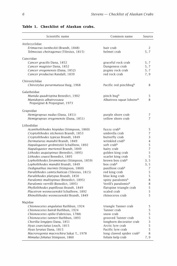
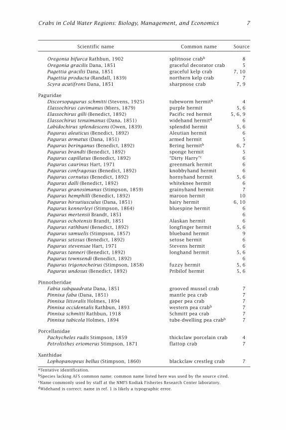
The list (Table 1) is ordered alphabetically by family, then by genusand species. The present list contains 11 families and 80 species of crabsthat have been identified in Alaskan waters. Among these, 28 species arehermit crabs (family Paguridae), 18 are stone crabs (family Lithodidae,including king crabs), 14 are spider crabs (family Majidae, including snowand Tanner crabs), and 6 are pea crabs (family Pinnotheridae). The squatlobsters (family Galatheidae) and pinchbugs (family Chirostylidae) are in-cluded because they are anomurans, like the Paguridae and Lithodidae.Perhaps more will be discovered in the near future.
Latin names denoted with a are tentative identifications. The commonnames are those accepted and published by the American Fisheries Society
6 Stevens — Checklist of Alaskan Crabs
Table 1. Checklist of Alaskan crabs.
Scientific name Common name Source
AtelecyclidaeErimacrus isenbeckii (Brandt, 1848) hair crab 2Telmessus cheiragonus (Tilesius, 1815) helmet crab 5, 7
CancridaeCancer gracilis Dana, 1852 graceful rock crab 5, 7Cancer magister Dana, 1852 Dungeness crab 5, 7Cancer oregonensis (Dana, 1852) pygmy rock crab 5, 7Cancer productus Randall, 1839 red rock crab 7, 9
ChirostylidaeChirostylus perarmatusa Haig, 1968 Pacific red pinchbugb 8
GalatheidaeMunida quadrispina Benedict, 1902 pinch bugb 5Munidopsis albatrossaea Albatross squat lobsterb 8 Pequegnat & Pequegnat, 1973
GrapsidaeHemigrapsus nudus (Dana, 1851) purple shore crab 7Hemigrapsus oregonensis (Dana, 1851) yellow shore crab 7
LithodidaeAcantholithodes hispidus (Stimpson, 1860) fuzzy crabb 5Cryptolithodes sitchensis Brandt, 1853 umbrella crab 7Cryptolithodes typicus Brandt, 1849 butterfly crab 3Dermaturus mandtii Brandt, 1849 wrinkled crabb 4Hapalogaster grebnitzkii Schalfeew, 1892 soft crabb 5Hapalogaster mertensii Brandt, 1849 hairy crab 7Lithodes aequispinus (Benedict, 1895) golden king crab 5Lithodes couesi Benedict, 1895 scarlet king crab 5Lopholithodes foraminatus (Stimpson, 1859) brown box crabb 3, 5Lopholithodes mandtii Brandt, 1849 box crabb 3, 5Oedignathus inermis (Stimpson, 1860) paxillose crabb 7Paralithodes camtschaticus (Tilesius, 1815) red king crab 5Paralithodes platypus Brandt, 1850 blue king crab 5Paralomis multispinus (Benedict, 1895) spiny paralomisb 8Paralomis verrilli (Benedict, 1895) Verill’s paralomisb 8Phyllolithodes papillosus Brandt, 1849 flatspine triangle crab 5Placetron wosnessenskii Schalfeew, 1892 scaled crab 5Rhinolithodes wosnessenskii Brandt, 1849 rhinoceros crab 5
MajidaeChionoecetes angulatus Rathbun, 1924 triangle Tanner crab 5Chionoecetes bairdi Rathbun, 1924 Tanner crab 5Chionoecetes opilio (Fabricius, 1788) snow crab 5Chionoecetes tanneri Rathbun, 1893 grooved Tanner crab 5Chorilia longipes Dana, 1851 longhorn decorator crab 3Hyas coarctatus Leach, 1815 Arctic lyre crab 5Hyas lyratus Dana, 1815 Pacific lyre crab 5Macroregonia macrochira Sakai T., 1978 long clawed spider crabb 8Mimulus foliatus Stimpson, 1860 foliate kelp crab 7, 9
Crabs in Cold Water Regions: Biology, Management, and Economics 7
Scientific name Common name Source
Oregonia bifurca Rathbun, 1902 splitnose crabb 8Oregonia gracilis Dana, 1851 graceful decorator crab 5Pugettia gracilis Dana, 1851 graceful kelp crab 7, 10Pugettia producta (Randall, 1839) northern kelp crab 7Scyra acutifrons Dana, 1851 sharpnose crab 7, 9
PaguridaeDiscorsopagurus schmitti (Stevens, 1925) tubeworm hermitb 4Elassochirus cavimanus (Miers, 1879) purple hermit 5, 6Elassochirus gilli (Benedict, 1892) Pacific red hermit 5, 6, 9Elassochirus tenuimanus (Dana, 1851) widehand hermitd 6Labidochirus splendescens (Owen, 1839) splendid hermit 5, 6Pagurus aleuticus (Benedict, 1892) Aleutian hermit 6Pagurus armatus (Dana, 1851) armed hermit 5Pagurus beringanus (Benedict, 1892) Bering hermitb 6, 7Pagurus brandti (Benedict, 1892) sponge hermit 5Pagurus capillatus (Benedict, 1892) “Dirty Harry”c 6Pagurus caurinus Hart, 1971 greenmark hermit 6Pagurus confragosus (Benedict, 1892) knobbyhand hermit 6Pagurus cornutus (Benedict, 1892) hornyhand hermit 5, 6Pagurus dalli (Benedict, 1892) whiteknee hermit 6Pagurus granosimanus (Stimpson, 1859) grainyhand hermit 7Pagurus hemphilli (Benedict, 1892) maroon hermit 10Pagurus hirsutiusculus (Dana, 1851) hairy hermit 6, 10Pagurus kennerleyi (Stimpson, 1864) bluespine hermit 6Pagurus mertensii Brandt, 1851 6Pagurus ochotensis Brandt, 1851 Alaskan hermit 6Pagurus rathbuni (Benedict, 1892) longfinger hermit 5, 6Pagurus samuelis (Stimpson, 1857) blueband hermit 9Pagurus setosus (Benedict, 1892) setose hermit 6Pagurus stevensae Hart, 1971 Stevens hermit 6Pagurus tanneri (Benedict, 1892) longhand hermit 5, 6Pagurus townsendi (Benedict, 1892) 6Pagurus trigonocheirus (Stimpson, 1858) fuzzy hermit 5, 6Pagurus undosus (Benedict, 1892) Pribilof hermit 5, 6
PinnotheridaeFabia subquadrata Dana, 1851 grooved mussel crab 7Pinnixa faba (Dana, 1851) mantle pea crab 7Pinnixa littoralis Holmes, 1894 gaper pea crab 7Pinnixa occidentalis Rathbun, 1893 western pea crabb 7Pinnixa schmitti Rathbun, 1918 Schmitt pea crab 7Pinnixa tubicola Holmes, 1894 tube-dwelling pea crabb 7
PorcellanidaePachycheles rudis Stimpson, 1859 thickclaw porcelain crab 4Petrolisthes eriomerus Stimpson, 1871 flattop crab 7
XanthidaeLophopanopeus bellus (Stimpson, 1860) blackclaw crestleg crab 7
aTentative identification.bSpecies lacking AFS common name; common name listed here was used by the source cited.cName commonly used by staff at the NMFS Kodiak Fisheries Research Center laboratory.dWidehand is correct; name in ref. 1 is likely a typographic error.
8 Stevens — Checklist of Alaskan Crabs
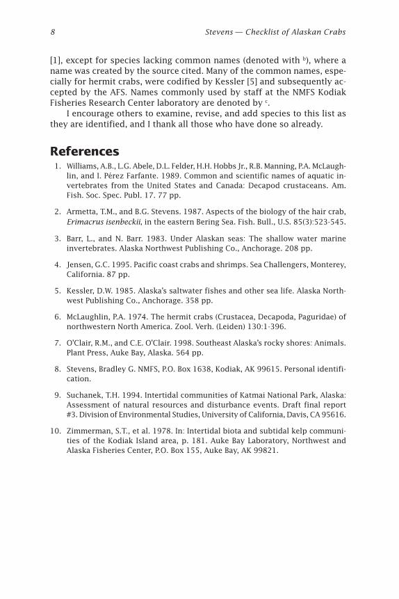
[1], except for species lacking common names (denoted with b), where aname was created by the source cited. Many of the common names, espe-cially for hermit crabs, were codified by Kessler [5] and subsequently ac-cepted by the AFS. Names commonly used by staff at the NMFS KodiakFisheries Research Center laboratory are denoted by c.
I encourage others to examine, revise, and add species to this list asthey are identified, and I thank all those who have done so already.
References 1. Williams, A.B., L.G. Abele, D.L. Felder, H.H. Hobbs Jr., R.B. Manning, P.A. McLaugh-
lin, and I. Pérez Farfante. 1989. Common and scientific names of aquatic in-vertebrates from the United States and Canada: Decapod crustaceans. Am.Fish. Soc. Spec. Publ. 17. 77 pp.
2. Armetta, T.M., and B.G. Stevens. 1987. Aspects of the biology of the hair crab,Erimacrus isenbeckii, in the eastern Bering Sea. Fish. Bull., U.S. 85(3):523-545.
3. Barr, L., and N. Barr. 1983. Under Alaskan seas: The shallow water marineinvertebrates. Alaska Northwest Publishing Co., Anchorage. 208 pp.
4. Jensen, G.C. 1995. Pacific coast crabs and shrimps. Sea Challengers, Monterey,California. 87 pp.
5. Kessler, D.W. 1985. Alaska’s saltwater fishes and other sea life. Alaska North-west Publishing Co., Anchorage. 358 pp.
6. McLaughlin, P.A. 1974. The hermit crabs (Crustacea, Decapoda, Paguridae) ofnorthwestern North America. Zool. Verh. (Leiden) 130:1-396.
7. O’Clair, R.M., and C.E. O’Clair. 1998. Southeast Alaska’s rocky shores: Animals.Plant Press, Auke Bay, Alaska. 564 pp.
8. Stevens, Bradley G. NMFS, P.O. Box 1638, Kodiak, AK 99615. Personal identifi-cation.
9. Suchanek, T.H. 1994. Intertidal communities of Katmai National Park, Alaska:Assessment of natural resources and disturbance events. Draft final report#3. Division of Environmental Studies, University of California, Davis, CA 95616.
10. Zimmerman, S.T., et al. 1978. In: Intertidal biota and subtidal kelp communi-ties of the Kodiak Island area, p. 181. Auke Bay Laboratory, Northwest andAlaska Fisheries Center, P.O. Box 155, Auke Bay, AK 99821.
Crabs in Cold Water Regions: Biology, Management, and Economics 9Alaska Sea Grant College Program • AK-SG-02-01, 2002
Setal Stage Duration of FemaleAdult Dungeness Crab(Cancer magister)Todd W. MillerOregon State University, Hatfield Marine Science Center, Department ofFisheries, Newport, Oregon
David G. HankinHumboldt State University, Department of Fisheries, Arcata, California
Extended AbstractThe Dungeness crab, Cancer magister, supports a significant commercialfishery between northern California and southeastern Alaska. Dynamicsof female C. magister molting patterns and their relation to growth andreproduction have been the subject of several studies (Wild 1980; Mohrand Hankin 1989; Hankin et al. 1989, 1997). The universal staging meth-ods of Drach (1939) and Drach and Tchernigovtzeff (1967) have not, how-ever, previously been applied to adult C. magister. Hatfield (1983) describedvarious stages of the molt cycle of C. magister larvae (megalopae), but herdescription of setal stages and stage durations does not apply to juvenilesor adults.
Adult female C. magister have a distinct annual molting period withmost activity occurring from February through May in northern California(Hankin et al. 1989). For crustaceans with distinct annual molting periods,setal molt staging can, in principle, be used to predict molting destiny ofindividual crabs prior to the annual molting season. Setal stages can onlybe used for this purpose; however, if it is determined that beyond a spe-cific molt stage molting is an “inevitable event” (e.g., a threshold stageafter which the crab must later molt). To be a reliable indicator of moltingdestiny, the expected number of days from entrance of this specific stageuntil molting must exceed the duration of the annual molting period (Mohrand Hankin 1989). If a sample were collected immediately prior to theannual molting season, then crabs staged at such a point or beyond wouldbe predicted to molt whereas other animals would not.
10 Miller and Hankin — Setal Stage Duration
Aiken (1973) used pleopods on the American lobster, Homarusamericanus, to describe premolt development and determined that moltpreparation could become arrested during setal stage D-0, with stage D-1¢being the earliest stage at which molting appeared “inevitable.” O’Halloranand O’Dor (1988), using maxilliped exopodites in the snow crab, Chionoecetesopilio, also found that D-1¢ was the earliest stage at which molting ap-peared inevitable. In this study, we used Drach and Tchernigovtzeff’s (1967)staging method to describe progression of premolt development, estimatedthe error in stage assignments, and estimated duration of individual moltstages.
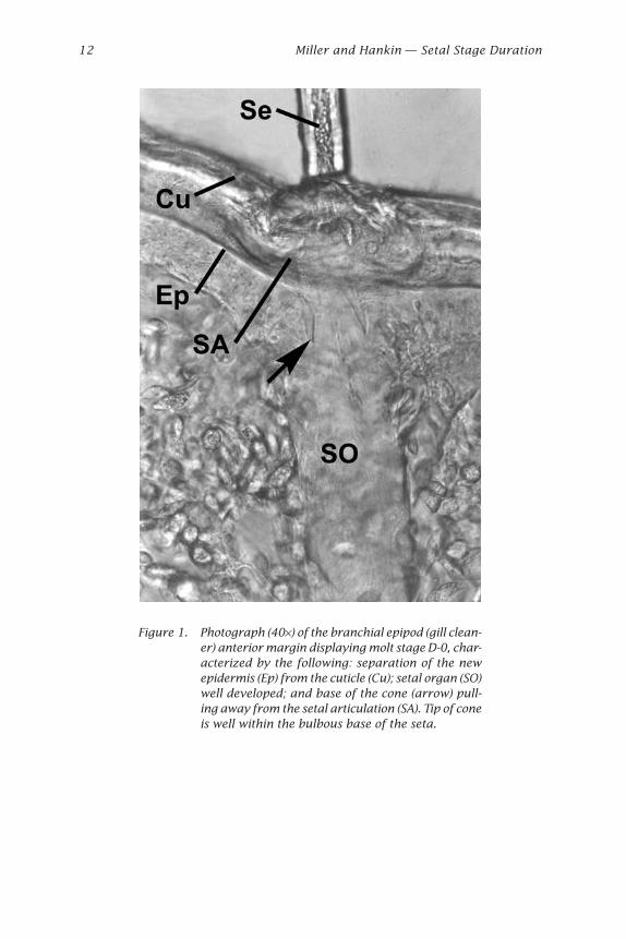
Using the general scheme of Drach and Tchernigovtzeff (1967), wewere able to identify intermolt stages (A1-C4) and premolt stages (D-0, D-1¢,D-1¢¢, D-1¢¢¢, and > D-2) of adult female C. magister based on setal develop-ment of branchial epipods (Table 1). One notable difference between ourobservations and those of Drach and Tchernigovtzeff (1967) is the ab-sence of a “cone” in the setal lumen during the late C4 stage. The cone wasonly apparent in C. magister at stage D-0, when retraction of the epider-mis revealed a cone partially within the bulbous base of the seta (Fig. 1).
We assessed the reliability of molt stage assignments by making threeindependent assignments of molt stage for a sample of 69 appendages.For each appendage, the “average” molt stage assigned was the most fre-quently assigned molt stage (i.e., 3 out of 3, or 2 out of 3 independentstagings) or the intermediate stage if an appendage received 3 differentstage assignments. For the kth molt stage an index of the error in assign-ment of that stage, Ik, was calculated using a modification of Beamish andFournier’s (1981) formula for estimation of error in aging fish:
Ik =
1 111N RX
kij
i
R
j
Nk
==Â
ÊËÁ
ˆ¯̃Â
where Nk is the number of appendages given average stage k, R is thenumber of times each appendage was staged, and Xij is the ith stage as-signment of the jth appendage:
(1) Xij = 0 if stage Xij is the same as the “average” stage (= k) of the jthappendage; or
(2) Xij = 1 if stage Xij is different than the “average” stage of the jth ap-pendage.
(Molt stage assignments were never more than one substage away fromthe average stage, k, over the three independent stagings.)
If all Nk appendages were each given three different assignments inthree sessions, then Ik would take on a maximum value of 1. If, instead, allNk appendages were given identical assignments in all sessions, then Ikwould take on its minimum value of 0. These indexes of errors in molt
Crabs in Cold Water Regions: Biology, Management, and Economics 11
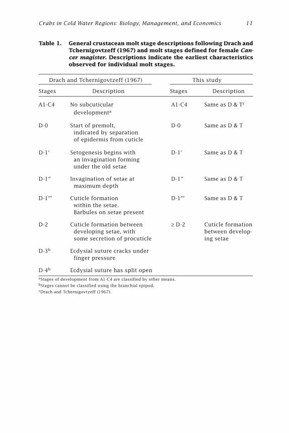
Table 1. General crustacean molt stage descriptions following Drach andTchernigovtzeff (1967) and molt stages defined for female Can-cer magister. Descriptions indicate the earliest characteristicsobserved for individual molt stages.
Drach and Tchernigovtzeff (1967) This study
Stages Description Stages Description
A1-C4 No subcuticular A1-C4 Same as D & Tc
developmenta
D-0 Start of premolt, D-0 Same as D & T indicated by separation of epidermis from cuticle
D-1¢ Setogenesis begins with D-1¢ Same as D & T an invagination forming under the old setae
D-1¢¢ Invagination of setae at D-1¢¢ Same as D & T maximum depth
D-1¢¢¢ Cuticle formation D-1¢¢¢ Same as D & T within the setae. Barbules on setae present
D-2 Cuticle formation between ≥ D-2 Cuticle formation developing setae, with between develop- some secretion of procuticle ing setae
D-3b Ecdysial suture cracks under finger pressure
D-4b Ecdysial suture has split openaStages of development from A1-C4 are classified by other means.bStages cannot be classified using the branchial epipod.cDrach and Tchernigovtzeff (1967).
12 Miller and Hankin — Setal Stage Duration
Figure 1. Photograph (40¥) of the branchial epipod (gill clean-er) anterior margin displaying molt stage D-0, char-acterized by the following: separation of the newepidermis (Ep) from the cuticle (Cu); setal organ (SO)well developed; and base of the cone (arrow) pull-ing away from the setal articulation (SA). Tip of coneis well within the bulbous base of the seta.
Crabs in Cold Water Regions: Biology, Management, and Economics 13
stage assignments could not be calculated for stages D-1¢¢¢ and ≥ D-2 dueto inaccessibility of crabs with those stages at the time of the experiment.Calculated errors in assignment of stages were 0.13, 0.18, and 0.19 forstages A1-C4, D-0, and D-1¢¢¢ respectively, but 0.06 for stage D-1¢¢. To ourknowledge this is the first time that reliability in assignments of molt stageshas been calculated.
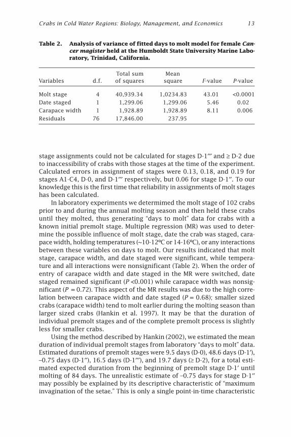
In laboratory experiments we determimed the molt stage of 102 crabsprior to and during the annual molting season and then held these crabsuntil they molted, thus generating “days to molt” data for crabs with aknown initial premolt stage. Multiple regression (MR) was used to deter-mine the possible influence of molt stage, date the crab was staged, cara-pace width, holding temperatures (~10-12ºC or 14-16ºC), or any interactionsbetween these variables on days to molt. Our results indicated that moltstage, carapace width, and date staged were significant, while tempera-ture and all interactions were nonsignificant (Table 2). When the order ofentry of carapace width and date staged in the MR were switched, datestaged remained significant (P <0.001) while carapace width was nonsig-nificant (P = 0.72). This aspect of the MR results was due to the high corre-lation between carapace width and date staged (P = 0.68); smaller sizedcrabs (carapace width) tend to molt earlier during the molting season thanlarger sized crabs (Hankin et al. 1997). It may be that the duration ofindividual premolt stages and of the complete premolt process is slightlyless for smaller crabs.
Using the method described by Hankin (2002), we estimated the meanduration of individual premolt stages from laboratory “days to molt” data.Estimated durations of premolt stages were 9.5 days (D-0), 48.6 days (D-1¢),–0.75 days (D-1¢¢), 16.5 days (D-1¢¢¢), and 19.7 days (≥ D-2), for a total esti-mated expected duration from the beginning of premolt stage D-1¢ untilmolting of 84 days. The unrealistic estimate of –0.75 days for stage D-1¢¢may possibly be explained by its descriptive characteristic of “maximuminvagination of the setae.” This is only a single point-in-time characteristic
Table 2. Analysis of variance of fitted days to molt model for female Can-cer magister held at the Humboldt State University Marine Labo-ratory, Trinidad, California.
Total sum MeanVariables d.f. of squares square F-value P-value
Molt stage 4 40,939.34 1,0234.83 43.01 <0.0001
Date staged 1 1,299.06 1,299.06 5.46 0.02
Carapace width 1 1,928.89 1,928.89 8.11 0.006
Residuals 76 17,846.00 237.95

14 Miller and Hankin — Setal Stage Duration
that would take a relatively short time to progress to the next stage. Wetherefore propose that stage D-1¢¢ is not a legitimate stage and should beconsidered only as an endpoint of stage D-1¢ leading into stage D-1¢¢¢.
Although experimental data thus showed that molting destiny of indi-vidual crabs could be predicted up to 84 days in advance of actual molt-ing, the typical duration of the molting season for female Dungeness crabsin northern California is approximately 120 days, substantially longer thanthe “notification time” achieved via molt staging. Molt stage descriptionand estimation of durations may still, however, have a utility in furtherunderstanding physiological processes involved in molting.
AcknowledgmentsWe would like to thank Dr. Bernard Sainte Marie for his input and com-ments on this research. Thanks to Humboldt State University TelonicherMarine Laboratory staff and Janet Webster (Oregon State University GuinLibrary). This paper is funded by a grant from the National Sea Grant Col-lege Program, National Oceanic and Atmospheric Administration, U.S. De-partment of Commerce through the California Sea Grant College System.The views expressed herein are those of the author(s) and do not neces-sarily reflect the views of NOAA or any of its subagencies. The U.S. Gov-ernment is authorized to reproduce and distribute for governmentalpurposes. This manuscript is dedicated to Arthur and Andrea Miller.
ReferencesAiken, D.E. 1973. Proecdysis, setal development, and molt prediction in the Amer-
ican lobster (Homarus americanus). J. Fish. Res. Board Can. 30:1337-1334.
Beamish, R.J., and D.A. Fournier. 1981. A method for comparing the precision of aset of age determinations. Can. J. Fish. Aquat. Sci. 38:982-983.
Drach, P. 1939. Mue et cycle d’intermue les Crustacea Decapodes. Ann. Inst. Oceanogr.19:103-392.
Drach, P., and C. Tchernigovtzeff. 1967. Sur la methode de determination des stadesd’intermue et son application generale aux crustaces. Vie et Milieu. Series A:Biol Mar. 18(3A):595-610. Translated to English in: Fish. Res. Board Can., Trans-lation Series No. 1296.
Hankin, D.G. 2002. Preliminary assessment of a new method to estimate durationof molt stages in crustaceans. In: A.J. Paul, E.G. Dawe, R. Elner, G.S. Jamieson,G.H. Kruse, R.S. Otto, B. Sainte-Marie, T.C. Shirley, and D. Woodby (eds.), Crabsin cold water regions: Biology, management, and economics. University ofAlaska Sea Grant, AK-SG-02-01, Fairbanks. (This volume.)
Hankin, D.G., T.H. Butler, P.W. Wild, and Q.L. Xue. 1997. Does intense fishing onmales impair mating success of female Dungeness crabs? Can. J. Fish. Aquat.Sci. 54(3):655-669.
Crabs in Cold Water Regions: Biology, Management, and Economics 15
Hankin, D.G., N. Diamond, M.S. Mohr, and J. Ianelli. 1989. Growth and reproductivedynamics of adult female Dungeness crabs (Cancer magister) in northern Cal-ifornia. J. Cons. Cons. Int. Explor. Mer 46:94-108.
Hatfield, S.E. 1983. Intermolt staging and distribution of Dungeness crab, Cancermagister, megalopae. In: P.W. Wild and R.N. Tasto (eds.), Life history, environ-ment, and mariculture studies of the Dungeness crab, Cancer magister, withemphasis on the central California fishery resource. Cal. Dept. Fish Game Fish.Bull. 172:85-96.
Mohr, M.S., and D.G. Hankin. 1989. Estimation of size-specific molting probabili-ties in adult decapod crustaceans based on postmolt indicator data. Can. J.Fish. Aquat. Sci. 46:1819-1830.
O’Halloran, M.J., and R.K. O’Dor. 1988. Molt cycle of male snow crabs, Chionoecetesopilio, from observations of external features, setal changes, and feeding be-havior. J. Crustac. Biol. 8(2):164-176.
Wild, P.W. 1980. Effects of seawater temperature on spawning, egg development,hatching success, and population fluctuations of the Dungeness crab, Cancermagister. Calif. Coop. Ocean. Fish. Investig. Rep. 21:115-120.

Crabs in Cold Water Regions: Biology, Management, and Economics 17Alaska Sea Grant College Program • AK-SG-02-01, 2002
Estimating Intermolt Duration inGiant Crabs (Pseudocarcinus gigas)Caleb GardnerTasmanian Aquaculture and Fisheries Institute, University of Tasmania,Tasmania, Australia
Andrew Jenkinson and Hendrik HeijnisAustralian Nuclear Science and Technology Organisation, Australia
AbstractEstimates of intermolt duration of giant crabs, based on tag-recapturemethodology, are used in evaluating management options. However, sev-eral shortcomings of tag-recovery data have been noted, including thelow number of tags inserted in legal-sized animals and the long periods oftime-at-large which require an unusually long intermolt duration. This ledto the evaluation of alternative methods to estimate intermolt duration.Reproduction in female giant crabs occurs in annual cycles, although fe-males occasionally “skip” a reproductive season and do not become oviger-ous; it has been noted previously that this appears to be associated withmolting. Thus the proportion of females that do not participate in repro-duction may indicate the proportion molting. We tried this approach witha sample of 342 females and measured the number that were “skipping” areproductive season by computerized tomography scanning (CT-scanning)of their ovaries prior to the extrusion of eggs. From the inferred propor-tion molting, intermolt duration was estimated at 9 years for mature sizeclasses; however, 95% confidence limits were broad (6.8-13.1 years). Thisestimate does, however, corroborate those previously reported from studiesin which tag and recapture methods were employed. Radiometric aging(228Th/ 228Ra) of carapaces was also undertaken with the focus of this workon testing an assumption of the method, rather than describing theintermolt duration of a population. We tested the assumption that there isnegligible exchange of radionuclides during intermolt in the exoskeleton,which is critical for reliable estimation of intermolt. SEM images of theinternal structure of the exoskeleton indicated that exchange of materialwithin the exoskeleton was unlikely and the majority of radiometric as-says were consistent with this observation. Radiometric age was estimated
18 Gardner et al. — Estimating Intermolt Duration
by gamma spectroscopy, which allowed rapid analysis compared to previ-ously reported methodology. This rapid processing may facilitate broaderapplication of radiometric aging to crustacean research.
IntroductionGiant crabs (Pseudocarcinus gigas) are fished across southern Australia ina small fishery based on high value live product. The fishery developedonly within the last decade, with negligible catch prior to 1991 (Gardner1998a). As a result, management is rudimentary in comparison to moreestablished fisheries in the region, notably that for the southern rock lob-ster (Jasus edwardsii). Although considerable research has been expendedon giant crabs, more information is required on their biology, includinggrowth. Growth influences most basic fisheries analyses, such as yield-and egg-per-recruit analyses, and is thus a high priority area for research.
General observations on molting of giant crabs were reported byLevings et al. (1996). They reported that males molt more frequently thanfemales, molting occurs in cycles longer than 1 year, and females producebroods over a range of instars (that is, there is no terminal molt to maturity).
Growth in crustaceans is a function of both the increase in size atmolt (molt increment) and the frequency of molting (intermolt duration).Molt increment in giant crabs has been estimated using data collectedthrough field based tag-recapture work with methods discussed by Levingset al. (1996). McGarvey et al. (1999; and R. McGarvey, South AustralianResearch and Development Institute, West Beach, Adelaide, South Australia,pers. comm.) modeled molt increment from the 350 recaptures in thisdata set that had molted at least once and quantified significant differ-ences in spatial patterns among both sexes in four states. They noted thatestimates of intermolt duration from tag recoveries require larger samplesizes than for quantifying the distribution of molt increments. This isbecause of the uncertainty around the time prior to the last molt for eachcrab tagged or recaptured.
Estimates of mean female intermolt by R. McGarvey et al. (pers. comm.)ranged from 4.5 years for immature females of 120 mm carapace length(CL) to 15 years for mature females of 180 mm CL. These estimates werebased on a discrete normal likelihood estimator, mean intermolt periodmodeled as a quadratic polynomial of premolt length. The analysis pooledall recaptures over a 5-year period from across southern Australia, as therewere insufficient data to differentiate regional trends. This analysis oftag-recapture data for intermolt duration by McGarvey et al. (1999) hasbeen used in assessing management of the Australian giant crab fishery,notably showing that the current legal minimum length for females isconservative, protecting about 50% of virgin population egg production.However, several shortcomings of tag recovery data from commercial fish-eries in giant crabs are noted. For instance, although most of the Austra-lian catch is taken in Tasmania, only 14 recaptures that had molted were
Crabs in Cold Water Regions: Biology, Management, and Economics 19
recorded from this state, with only 2 of these from males. Limitations oftagging for estimating intermolt duration of giant crabs are threefold: (1)Because giant crabs are high value and numbers captured are low, tagsinserted in the course of commercial fishing operations have been placedalmost solely in giant crabs that are protected and must therefore be le-gally returned to the sea. These are crabs below the legal minimum lengthof 150 mm CL, and ovigerous females. Tags have thus rarely been placed inlegal size animals. (2) The unusually long intermolt duration of giant crabsrequires corresponding long times-at-large. (3) Uncertainty remains, as withall tag-recovery intermolt period estimators, about the time back to themost recent molt prior to first capture.
We assessed three alternative methods for study of growth in giantcrabs: (1) inferring the proportion of the population molting based on theproportion of females participating in reproduction; (2) radiometric agingof the exoskeleton; and (3) lipofuscin aging. Although lipofuscin aging is arelatively new technique, it has been studied intensively and methods aredescribed in detail elsewhere (Sheehy 1992, Wahle et al. 1996, Sheehy etal. 1998). Consequently, in this paper we focus on the first two methods,which have been applied less widely.
Reproductive State of FemalesFemale giant crabs produce clutches of eggs in annual cycles with femalesextruding eggs in late autumn that hatch in spring, although not all fe-males participate in egg production each year (Levings et al. 1996, Gardner1997). “Skipping” of reproduction by females may occur in years before orafter molting, based on observations in tank trials and also through com-paring fouling state of shells with ovigerous state of females (Gardner1998b, McGarvey et al. 1999). This relationship between molting and skip-ping of reproduction implies that a measure of intermolt duration couldbe obtained from the proportion of females skipping reproduction in any1 year. For instance, if half the population were found to skip reproduc-tion in any 1 year, it would suggest that molting occurred every 2 years.
Radiometric AgingResearch on the radiometric aging of calcified biological structures has beenundertaken sporadically for several decades with several studies focusedon crustaceans (Bennett and Turekian 1984, Le Foll et al. 1989, Nevissi etal. 1996). The application of radiometric aging to crustaceans is based onthe incorporation of radium (228Ra) with calcium into the exoskeleton aftermolting; this radium thereafter decays to thorium (228Th). Several meth-ods to measure nuclear decay in biological samples have been describedincluding alpha-spectroscopy, thermal ionization mass spectrometry, andgamma-spectroscopy (Bennett and Turekian 1984, Reyss et al. 1995,Andrews et al. 1999). Various methods differ in the accuracy of their ageestimation and also in time and expense required to process samples;
20 Gardner et al. — Estimating Intermolt Duration
however, the fundamental principle for the estimation of age throughnuclear decay sequences remains consistent. An aspect of radiometricaging that has caused greater concern among many biologists is the valid-ity of assumptions made in radiometric age determination. These wereoutlined by Nevissi et al. (1996) as: “(1) during molting virtually all thecalcium and associated nuclides are lost by the animal; (2) the carapace iscalcified rapidly after molting, so that (3) addition or removal of radionu-clides during the intermolt period is negligible.”
Similar assumptions to those outlined by Nevissi et al. (1996) exist withall applications of radiometric aging for biological samples, yet they areseldom tested. Fenton et al. (1990) showed that an assumption of con-stant accumulation of 226Ra into otoliths of a finfish, the blue grenadier(Macruronus novaezelandiae), was violated and thus radiometric agingcould not be applied. Le Foll et al. (1989) used radiometric techniques toestimate the age of crustacean exoskeletons of known age, which pro-vided a test of the extent of any addition or removal of radionuclidesduring the intermolt. Although they found reasonable agreement, somediscrepancies were noted at extremes. We also examined the assumptionof negligible addition or removal of radionuclides during the intermoltperiod in giant crabs by comparing age estimates for inner, middle, andouter layers of the carapace.
MethodsProportion of Females ReproducingA total of 342 female giant crabs were collected in April 1998 by a com-mercial fisher from areas adjacent to Bicheno off Tasmania’s east coast.Sizes were from 92 to 208 mm CL, with the majority of animals (N = 327)larger than the size at 50% onset of maturity for this region, approximately135 mm CL (Levings et al. 2001). This sample was collected prior to fe-males extruding their eggs, which typically occurs in May (Gardner 1997).Fishers confirmed that no ovigerous females had been observed along thecoast during the month of April. Samples were collected prior to oviposi-tion to avoid bias in the ratio of reproductively active to inactive females,as ovigerous females have reduced catchability (Gardner 1998a).
The proportion of females in this sample that were reproductivelyactive in the current year was assessed by the extent of ovarian develop-ment. Ovaries and spermathecae were viewed nondestructively using aGM™ computerized tomography scanner (CT-scanner; Gardner et al. 1998).Forty specimens were individually tagged and retained in tanks for a fur-ther 2 months until after oviposition to validate the ovarian classifica-tions from the CT-scans. Ten animals were held in each 4 m3 tank, whichwere equipped with flow-through seawater supply and a sand substrate,approximately 150 mm deep, to assist in oviposition.
The proportion of females without developing ovaries was used as anindicator of the proportion molting by calculating the ratio of females without
Crabs in Cold Water Regions: Biology, Management, and Economics 21
developing ovaries relative to those with developing ovaries. Confidence limitsof this estimate were obtained by bootstrapping using 10,000 simulations.
Test of Assumptions of Radiometric AgingSix male giant crabs were captured from areas adjacent to Bicheno offTasmania’s east coast by a commercial fisher. Each specimen had shellwith heavy wear (carapace-condition 3 in Gardner [1997]) and ranged be-tween 199 and 223 mm CL. Large males were selected for this componentdue to their thick carapaces, which facilitated separation of the shell intodifferent layers and the collection of large amounts of material. Radiometricanalyses were by gamma spectroscopy, which is more rapid with largersamples.
The potential for addition or removal of radionuclides during theintermolt period was initially investigated by viewing the internal struc-ture of the exoskeleton. Scanning electron microscopy (SEM) images wereacquired in environmental mode with an ElectroScan™ ESEM2020 usingwater vapor as the imaging gas. The specimen chamber pressure wasmaintained at 5.0 torr.
Testing of the extent of exchange of radionuclides during the intermoltperiod by radiometric analysis was based on the hypothesis that materialexchange would not occur uniformly through the exoskeleton. If exchangeof radionuclides occurred between the exoskeleton and internal tissues,then we would expect younger age estimates from inner layers. Likewise,if exchange occurred with the environment, then age estimates from outerlayers would be younger than those from the middle or inner layers.
Radiometric analysis was by gamma spectroscopy which avoided thechemical ingrowth stages described by Nevissi et al. (1996), although theprinciple of estimation through the analysis of the 228Th/ 228Ra ratio remainedthe same. Samples of the exoskeleton were prepared for analysis by grind-ing with hand-held grinder (Dremmel™) using a rotating tungsten steel bit.This was intended to separate material into coarse inner, middle, and outerlayers of the exoskeleton, rather than anatomical layers of the integument.Samples were ground further in a standard ring mill prior to radiometricanalyses, then weighed accurately into 55 ml Petri dishes to completely fillthe dish. Due to the absence of any prolonged gaseous stage in the decom-position chain, processing did not involve any steps of prolonged sealing.Samples were measured on a high-resolution Compton suppression gamma-ray spectrometer (Canberra Industries, Meriden, USA). The spectrometerconsisted of an n-type high-purity germanium (HPGe) coaxial detector withrelative efficiency of 50% surrounded by a sodium iodide (NaI) annularguard detector and removable NaI “plug” detector. The detector assemblywas housed in a graded lead shield. Data analysis was performed usingGENIE2000 software developed by Canberra Industries (Meriden, USA).
The activity of 228Ra was determined by measuring its daughter 228Acat 911 keV and the activity of 228Th was determined by its progeny 212Pb at
22 Gardner et al. — Estimating Intermolt Duration
238 keV (Reyss et al. 1995). The age of the specimen was then determinedaccording to the following equation:
Age of carapace at death = (Isotopic Age) – (time between death andmeasurement)where:
Isotopic Age
Activity of ThActivity of Ra
= - ¥ - ¥È
ÎÍ
˘
˚˙4 12 1 0 669
228
228. .
( )( )
Ln
Isotopic Age is in years.
ResultsProportion of Females ReproducingRetention of a subsample of 40 individually tagged female crabs in tanksafter CT-scanning confirmed that the 35 females classed as possessingdeveloping ovaries went on to extrude eggs, while the remaining 5 fe-males with ovaries classed as undeveloped did not extrude eggs. Thisstep validated the use of CT-scanning of ovaries for estimating the pro-portion of the sample that would reproduce in the current year.
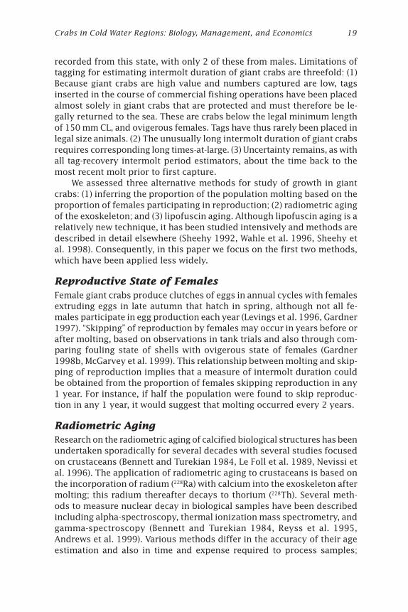
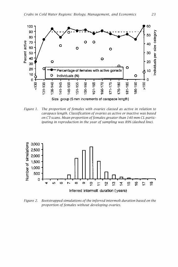
Only two females did not appear to have mated, based on the appear-ance of the spermathecae; each of these were relatively small (92 and 142mm CL). The proportion of females that were reproducing in the currentyear was lowest in smaller size categories, although stabilized in sizeclasses greater than 140 mm CL (Fig. 1). The mean proportion of femalesthat were not reproducing for all size classes greater than 140 mm CLpooled was 11%, which equates to approximately 1 in 9 (N = 327). Assum-ing the apparent link between molting and skipping reproduction holdstrue, this implies an intermolt period of 9 years for female giant crabsgreater than 140 mm CL.
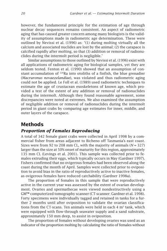
Estimates obtained by this indirect method of estimating intermoltduration appear affected by the constraining upper limit of 100% maturityof females. That is, random error around the estimate of the proportionreproducing appears to have a large influence on the estimate of intermoltduration. This is shown by the bootstrapped estimates of inferred intermoltduration which have a broad range (Fig. 2; lower 95% confidence limit =6.81 years, upper = 13.08 years).
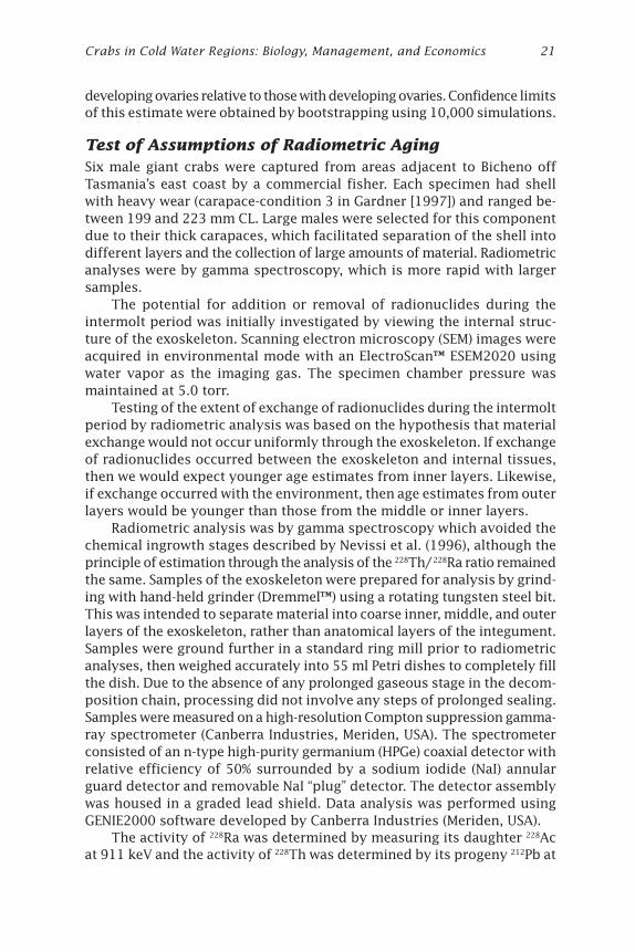
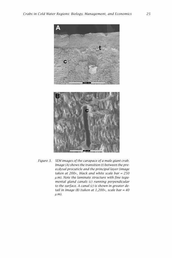
Test of Assumptions of Radiometric AgingThe validity of the assumption of no addition or removal of radionuclidesduring intermolt was initially assessed by viewing samples of the cara-pace in cross section using SEM. General structure of the exoskeleton wassimilar to that described by Stevenson (1985) with the epicuticle, pre-ecdysalprocuticle, and principal layer of the procuticle calcified and formed oflaminae parallel with the surface (Fig. 3A). Fine canals of around 2 mm indiameter run perpendicular to the surface and appeared to be associated
Crabs in Cold Water Regions: Biology, Management, and Economics 23
Figure 1. The proportion of females with ovaries classed as active in relation tocarapace length. Classification of ovaries as active or inactive was basedon CT-scans. Mean proportion of females greater than 140 mm CL partic-ipating in reproduction in the year of sampling was 89% (dashed line).
Figure 2. Bootstrapped simulations of the inferred intermolt duration based on theproportion of females without developing ovaries.
24 Gardner et al. — Estimating Intermolt Duration
with tegumental glands (Fig. 3B). No structures that suggest that materialis exchanged within the carapace were present, such as the canaliculi in-volved in cycling of mammalian bone (Junqueira and Carneiro 1983).
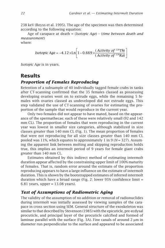
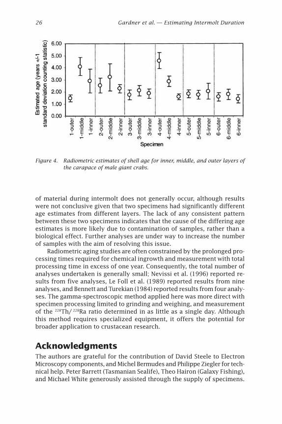
Radiometric results presented here are preliminary as they are basedon only 18 analyses (3 layers for each of 6 crabs; Fig. 4) and further analy-ses are in progress. Estimates for these individuals ranged between 2 and5 years. Although the sample size is small, there appears to be no signifi-cant difference in age estimates between layers in most specimens. Thissuggests that there was no material exchanged within the carapace duringintermolt. In contrast, different age estimates between layers were ob-served in two specimens (numbers 1 and 4). There was no systematicpattern between these sets of analyses; in one case the oldest estimatewas from the outer layer, while the youngest estimate was from the outerlayer in the other.
DiscussionThe methods assessed here may contribute to our understanding ofintermolt duration based on tag-recapture data. Measurement of the pro-portion of females reproducing produced intermolt duration estimates ofaround 9 years, although confidence limits were broad (ranging from 6.8to 13.1 years). This estimate of intermolt duration corroborates that ob-tained from tagging data (McGarvey et al. 1999) and provides support forthe conclusion of an exceptionally long intermolt duration in female giantcrabs. The robust carapace of giant crabs, which can exceed 4 mm in thick-ness, also testifies to a protracted intermolt period.
The use of the proportion of females participating in reproduction toestimate intermolt could only be applied to species meeting a specializedset of criteria. These criteria include a well-defined reproductive seasonand the linking of molting to the reproductive cycle so that the two eventsare mutually exclusive. Estimates will have greater precision where theproportion of animals that are participating in reproduction does not ap-proach the 0% or 100% bounds. This implies greatest precision wheremolting occurs every 2 or 3 years (closer to 50% of animals molting eachyear), rather than the more protracted intermolt of giant crabs which ledto broader confidence limits around estimates.
Radiometric estimates of male intermolt period also corroborate dataobtained through tagging. Our estimates from individual analyses of crabs,which all had worn carapaces, ranged between 2 and 5 years while McGarveyet al. (1999) estimated intermolt from tagging data to be around 4 years.
We attempted to evaluate the potential for error in these estimates ofradiometric age caused by exchange of material during intermolt. Themicroscopic structure of the exoskeleton would suggest that regular turn-over of material within the exoskeleton is unlikely, which is consistentwith the process of endocuticle synthesis described by Stevenson (1985)and Skinner et al. (1992). Radiometric analyses also indicated that exchange
Crabs in Cold Water Regions: Biology, Management, and Economics 25
Figure 3. SEM images of the carapace of a male giant crab.Image (A) shows the transition (t) between the pre-ecdysal procuticle and the principal layer (imagetaken at 200× , black and white scale bar = 250µm). Note the laminate structure with fine tegu-mental gland canals (c) running perpendicularto the surface. A canal (c) is shown in greater de-tail in image (B) (taken at 1,200× , scale bar = 40µm).
26 Gardner et al. — Estimating Intermolt Duration
of material during intermolt does not generally occur, although resultswere not conclusive given that two specimens had significantly differentage estimates from different layers. The lack of any consistent patternbetween these two specimens indicates that the cause of the differing ageestimates is more likely due to contamination of samples, rather than abiological effect. Further analyses are under way to increase the numberof samples with the aim of resolving this issue.
Radiometric aging studies are often constrained by the prolonged pro-cessing times required for chemical ingrowth and measurement with totalprocessing time in excess of one year. Consequently, the total number ofanalyses undertaken is generally small; Nevissi et al. (1996) reported re-sults from five analyses, Le Foll et al. (1989) reported results from nineanalyses, and Bennett and Turekian (1984) reported results from four analy-ses. The gamma-spectroscopic method applied here was more direct withspecimen processing limited to grinding and weighing, and measurementof the 228Th/ 228Ra ratio determined in as little as a single day. Althoughthis method requires specialized equipment, it offers the potential forbroader application to crustacean research.
AcknowledgmentsThe authors are grateful for the contribution of David Steele to ElectronMicroscopy components, and Michel Bermudes and Philippe Ziegler for tech-nical help. Peter Barrett (Tasmanian Sealife), Theo Hairon (Galaxy Fishing),and Michael White generously assisted through the supply of specimens.
Figure 4. Radiometric estimates of shell age for inner, middle, and outer layers ofthe carapace of male giant crabs.
Crabs in Cold Water Regions: Biology, Management, and Economics 27
Jean Louis Reyss and Daniel Latrouite provided advice on gamma spec-troscopy. Hobart Radiology donated CT-scanning equipment and staff timeto the project. Rick McGarvey helped improve the manuscript. Financialsupport was provided by the Australian Institute of Nuclear Science andEnergy, the Australian Research Council, The Tasmanian Department ofPrimary Industry and Fisheries, and the Tasmanian giant crab industry.
ReferencesAndrews, A.H., K.H. Coale, J.L. Nowicki, C. Lundstrom, Z. Palacz, E.J. Burton, and
G.M. Cailliet. 1999. Application of an ion-exchange separation technique andthermal ionization mass spectroscopy to 226Ra determination of long-lived fish-es. Can. J. Fish. Aquat. Sci. 56:1329-1338.
Bennett, J.T., and K.K. Turekian. 1984. Radiometric ages of brachyuran crabs fromthe Galapagos spreading-centre hydrothermal ventfield. Limnol. Oceanogr.29:1088-1091.
Fenton, G.E., D.A. Ritz, and S.A. Short. 1990. 210Pb/226Ra disequilibria in otoliths ofblue grenadier, Macruronus novaezelandiae; problems associated with radio-metric ageing. Aust. J. Mar. Freshw. Res. 41:467-473.
Gardner, C. 1997. Effect of size on reproductive output of giant crabs Pseudocarci-nus gigas (Lamarck): Oziidae. Aust. J. Mar. Freshw. Res. 48:581-587.
Gardner, C. 1998a. The Tasmanian giant crab fishery: A synopsis of biological andfisheries information. Tasmanian Department of Primary Industry and Fisher-ies Report 43. 40 pp.
Gardner, C. 1998b. The larval and reproductive biology of the giant crab. Ph.D.thesis, University of Tasmania, Hobart, Tasmania, 333 pp.
Gardner, C., M. Rush, and T. Bevilacqua. 1998. Nonlethal imaging techniques forcrab spermathecae. J. Crustac. Biol. 18:64-69.
Junqueira, L.C., and J. Carneiro. 1983. Basic histology, 4th edition. Lange MedicalPublications, Los Altos, California. 510 pp.
Le Foll, D., E. Brichett, J.L. Reyss, C. Lalou, and D. Latrouite. 1989. Age determina-tion of the spider crab Maja squinado and the European lobster Homarus gam-marus by 228Th/ 228Ra chronology: Possible extension to other crustaceans.Can. J. Fish. Aquat. Sci. 46:720-724.
Levings, A., B.D. Mitchell, T. Heeren, C. Austin, and J. Matheson. 1996. Fisheriesbiology of the giant crab (Pseudocarcinus gigas, Brachyura, Oziidae) in south-ern Australia. In: High latitude crabs: Biology, management, and economics.University of Alaska Sea Grant, AK-SG-96-02, Fairbanks, pp. 125-151.
Levings, A., B.D. Mitchell, R. McGarvey, J. Matthews, L. Laurenson, C. Austin, T.Heeren, N. Murphy, A. Miller, M. Rowsell, and P. Jones. 2001. Fisheries biologyof the giant crab (Pseudocarcinus gigas). Final report to the Fisheries Researchand Development Corporation, 93/220 and 97/132. 388 pp.
28 Gardner et al. — Estimating Intermolt Duration
McGarvey, R., J.M. Matthews, and A.H. Levings. 1999. Yield-, value-, and egg-per-recruit of giant crab, Pseudocarcinus gigas. South Australian Research andDevelopment Institute Report. 73 pp.
Nevissi, A., J.M. Orensanz, A.J. Paul, and D.A. Armstrong. 1996. Radiometric esti-mation of shell age in Chionoecetes spp. from the eastern Bering Sea, and itsuse to interpret shell condition indices: Preliminary results. In: High latitudecrabs: Biology, management, and economics. University of Alaska Sea Grant,AK-SG-96-02, Fairbanks, pp. 389-396.
Reyss, J.L., S. Schmidt, F. Legeleux, and P. Bonte.1995. Large, low background well-type detectors for measurements of environmental radioactivity. Nucl. Instr.and Meth. in Phys. Res. A 357:391-397.
Sheehy, M.R.J. 1992. Lipofuscin age-pigment accumulation in the brains of ageingfield- and laboratory-reared crayfish Cherax quadricarinatus (von Martens)(Decapoda: Parastacidae). J. Exp. Mar. Biol. Ecol. 161:79-89.
Sheehy, M., N. Caputi, C. Chubb, and M. Belchier. 1998. Use of lipofuscin for resolv-ing cohorts of western rock lobster (Panulirus cygnus). Can. J. Fish. Aquat. Sci.55:925-936.
Skinner, D.M., S.S. Kumari, and J.J. O’Brien. 1992. Proteins of the crustacean exo-skeleton. Am. Zool. 32:470-484.
Stevenson, J.R. 1985. Dynamics of the integument. In: D.E. Bliss and L.H. Mantel(eds.), The biology of Crustacea, Vol. 9. Academic Press, New York, pp. 1-42.
Wahle, R.A., O. Tully, and V. O’Donovan. 1996. Lipofuscin as an indicator of age incrustaceans: Analysis of the pigment in the American lobster Homarus amer-icanus. Mar. Ecol. Prog. Ser. 138:117-123.
Crabs in Cold Water Regions: Biology, Management, and Economics 29Alaska Sea Grant College Program • AK-SG-02-01, 2002
Molting of Red King Crab(Paralithodes camtschaticus)Observed by Time-Lapse Videoin the LaboratoryBradley G. StevensNational Marine Fisheries Service, Kodiak Fisheries Research Center,Kodiak, Alaska
AbstractMolting of six red king crabs was observed and recorded on time-lapsevideo in January 2000. Three molted during daytime, and three at nightunder dark red light. A suite of 16 behaviors were exhibited during the 6hours prior to and one hour after molting, including two behaviors notpreviously observed: body shaking and leg pumping. During leg pump-ing, the crab alternately contracted and extended the legs causing the newexoskeleton to bend and fold, thus shortening the legs to enable theirextraction from the old exoskeleton. Average time required for ecdysis,from splitting the carapace to complete extrication, was 0.34 hour (20minutes, 17 seconds).
IntroductionAmong all animals, the growth process of the Arthropoda is unique becauseof the requirement for ecdysis, or molting of the exoskeleton. In crusta-ceans, this process has been fairly well studied from a metabolic and physi-ological point of view, as reviewed by Skinner (1985). The stages of ecdysiswere initially defined by Drach (1939) based on exoskeleton hardness, thenlater redefined by Skinner (1962) on the basis of subcuticular cellular pro-cesses. The longest stage is the intermolt, or anecdysial period (stage C4).During this period, molt inhibiting hormone (MIH) is secreted by the X-organ/sinus gland complex of the eyestalk, preventing ecdysis (Skinner1985). Cessation of MIH release, usually in response to environmental stimuli,allows production and release of molting hormone (MH, or a-ecdysone)from the Y-organ, stimulating ecdysis. Molting begins with proecdysis,
30 Stevens — Molting of Red King Crab
during which ecdysone is released, and somatic muscles atrophy (D0), theold exoskeleton is reabsorbed (D1), epidermal cells enlarge and secrete anew cuticle (D2-D3), and astaxanthin is resorbed from the cuticle into theblood (D4). Ecdysis (stage E) occurs when the carapace splits at the epimeralline, and the animal withdraws from the old exoskeleton. During the fol-lowing stages, termed metecdysis, the epidermal cells shrink (A), muscleis synthesized (B), endocuticle is formed (C1-C3), and the shell hardens.
The stages of ecdysis and early metecdysis are probably the mostvulnerable periods in the life of a crustacean. During this brief interval,the muscles are weakened, the animal may be trapped halfway out of theold exoskeleton, it may be blinded, and the soft new cuticle provides littleprotection from predators. It is therefore surprising that few studies havebeen conducted on the behavioral aspects of molting. For the red kingcrab (Paralithodes camtschaticus) there is evidence that adults cease feed-ing up to 3 weeks prior to molting, and do not resume feeding until morethan a week afterwards (Zhou et al. 1998). First- through fourth-stage ju-venile red king crabs spend more time in sheltered habitats than on opensand during periods of molting (B.G. Stevens, unpubl. data). However, thephysical act of molting has rarely been documented.
The commercial value and size of king crabs makes them particularlyworthwhile subjects for studies of molting. Predation of crabs duringmolting is a common subject of speculation and hyperbole among com-mercial fishermen. Recently molted red king crabs are occasionally foundin the stomachs of large predatory fish such as Pacific cod (Gadus macro-cephalus) and Pacific halibut (Hippoglossus stenolepis), leading many fish-ermen to blame them for the demise of local crab populations. Over geologictime scales, crustaceans must have developed adaptive behaviors whichlessen the likelihood of molt-associated mortality. This study was con-ducted in order to better understand the behavioral aspects of molting inred king crab. Specific questions of interest were: How long does it take?When does it occur? Are specialized behaviors involved? What problemscan arise during molting? And not least of all, it seemed worthwhile torecord the process on video for research and educational purposes.
Materials and MethodsRed king crabs were captured by scuba divers and brought to the labora-tory, where they were measured and tagged with a numbered Petersondisk tag attached to a plastic cable-tie wrapped around the third right leg.Crabs were held in two 500 liter tanks, fed twice weekly with squid, andobserved daily until they showed signs of molting. About 24 hours priorto molting the abdomen began to swell, from its normal thickness at theedge of about 1-2 mm, to a thickness of about 5-10 mm. The crab was thenplaced into a 200 liter tank (dimensions 0.5 ¥ 0.5 ¥ 0.65 m) containingrunning filtered seawater and a gravel-covered bottom. A waterproof blackand white video camera was suspended in the tank so that it viewed 90%
Crabs in Cold Water Regions: Biology, Management, and Economics 31
of the tank bottom. The tank was illuminated indirectly by a white fluores-cent light from 0700 to 1700, and by dark red light from 1700 to 0700 (L:Dratio of 10:14). The camera signal was recorded on a time lapse VCR(Panasonic AG6550) running in continuous 24 hour mode (actual time com-pression ratio was 13:1). Crabs were checked periodically to determinewhen molting occurred. If the crab had not completed molting within 24hours, the tape was rewound and restarted.
Recorded videotapes were converted to an MPEG type digital videofile, and analyzed using “The Observer Video-Pro” software (Noldus Cor-poration, Netherlands). Individual behavior codes were assigned to key-board characters, so that the computer recorded the behavior code, videoframe number, and time (to the nearest 0.1 second) whenever a key waspressed. Independent variables recorded were species, sex, tag number,and date and time that the time-lapse recording was started. Behavioralobservations were of two types: events and states. Events (Table 1) wereshort discrete behaviors for which only the start time was recorded. Someevents had modifiers describing the event. States (Table 2) were longer-lasting but nonoverlapping behaviors, which lasted until the next behav-ioral state occurred. Events could occur within states. Descriptions of theevents, states, and modifiers are listed in Tables 1 and 2.
Most crabs were in the observation tank for more than a day beforemolting, although some molted within a few hours. For this reason, thelength of observation varied for each crab. In order to standardize as muchas possible, only the last 6 hours of the time-lapse video prior to moltingwas analyzed for most crabs. This period is about equivalent to the dura-tion of molt stage D4.
ResultsVideotaped observations were made for six crabs in January of 2000. Twocrabs were females, and four were males; sizes ranged from 82 to 102 mmcarapace length (CL; Table 3). Although “Leg out,” “Abdomen,” and “Molt”with their associated modifiers were used to describe specific stages ofthe molting process, they are not behaviors per se. Shove, Tilt, Rest, Rock,Push, Walk, Move legs, Rotate, and Stand/sit are normal behaviors that areused in other contexts besides molting; they were probably associatedwith finding a “comfortable” place and position in which to begin moltingand may not be part of the molting process itself. Pump body and Pumplegs were behaviors that were strictly associated with the act of ecdysisand did not occur in any other context. Shaking, although it began up to 6hours prior to molting, is not a behavior exhibited by crabs at any othertime, and was never observed prior to this study.
Figures 1A and 1B illustrate the behaviors of two crabs from 5 hoursbefore molting to about 1 hour after. These two were selected because oftheir similarity in general behavior pattern, length of observation time, andsimilarity to mean data (see Fig. 2). The following is a general description
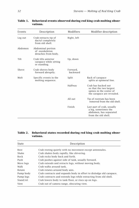
32 Stevens — Molting of Red King Crab
Table 1. Behavioral events observed during red king crab molting obser-vations.
Events Description Modifiers Modifier description
Leg out Crab extracts tip of Right, left dactyl completely from old shell.
Abdomen Abdominal portion of exoskeleton detaches from body.
Tilt Crab tilts anterior Up, down carapace while sitting or standing.
Shove Crab shoves body Forward, forward abruptly. backward
Molt Specific events in the Split Back of carapace molting sequence. splits at epimeral line.
Halfway Crab has backed out so that the two largest spines in the center of the carapace are revealed.
All out Tip of rostrum has been removed from the old shell.
Finish Last part of crab, usually a leg, sometimes the abdomen, has separated from the old shell.
Table 2. Behavioral states recorded during red king crab molting obser-vations.
State Description
Rest Crab resting quietly with no movement except antennules.
Shake Crab shakes body rapidly, like shivering.
Rock Crab rocks body back and forth.
Push Crab pushes against side of tank, usually forward.
Move legs Crab extends and retracts legs, without moving body.
Walk Crab walks around tank.
Rotate Crab rotates around body axis.
Pump body Crab contracts and expands body in effort to dislodge old carapace.
Pump legs Crab contracts and extends legs while extracting from old shell.
Stand/sit Crab lowers body to tank floor, or rises up on legs.
View Crab out of camera range, obscuring view.
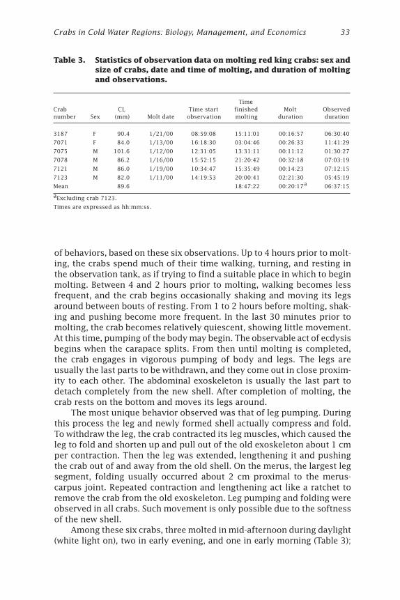
Crabs in Cold Water Regions: Biology, Management, and Economics 33
of behaviors, based on these six observations. Up to 4 hours prior to molt-ing, the crabs spend much of their time walking, turning, and resting inthe observation tank, as if trying to find a suitable place in which to beginmolting. Between 4 and 2 hours prior to molting, walking becomes lessfrequent, and the crab begins occasionally shaking and moving its legsaround between bouts of resting. From 1 to 2 hours before molting, shak-ing and pushing become more frequent. In the last 30 minutes prior tomolting, the crab becomes relatively quiescent, showing little movement.At this time, pumping of the body may begin. The observable act of ecdysisbegins when the carapace splits. From then until molting is completed,the crab engages in vigorous pumping of body and legs. The legs areusually the last parts to be withdrawn, and they come out in close proxim-ity to each other. The abdominal exoskeleton is usually the last part todetach completely from the new shell. After completion of molting, thecrab rests on the bottom and moves its legs around.
The most unique behavior observed was that of leg pumping. Duringthis process the leg and newly formed shell actually compress and fold.To withdraw the leg, the crab contracted its leg muscles, which caused theleg to fold and shorten up and pull out of the old exoskeleton about 1 cmper contraction. Then the leg was extended, lengthening it and pushingthe crab out of and away from the old shell. On the merus, the largest legsegment, folding usually occurred about 2 cm proximal to the merus-carpus joint. Repeated contraction and lengthening act like a ratchet toremove the crab from the old exoskeleton. Leg pumping and folding wereobserved in all crabs. Such movement is only possible due to the softnessof the new shell.
Among these six crabs, three molted in mid-afternoon during daylight(white light on), two in early evening, and one in early morning (Table 3);
Table 3. Statistics of observation data on molting red king crabs: sex andsize of crabs, date and time of molting, and duration of moltingand observations.
TimeCrab CL Time start finished Molt Observednumber Sex (mm) Molt date observation molting duration duration
3187 F 90.4 1/21/00 08:59:08 15:11:01 00:16:57 06:30:40
7071 F 84.0 1/13/00 16:18:30 03:04:46 00:26:33 11:41:29
7075 M 101.6 1/12/00 12:31:05 13:31:11 00:11:12 01:30:27
7078 M 86.2 1/16/00 15:52:15 21:20:42 00:32:18 07:03:19
7121 M 86.0 1/19/00 10:34:47 15:35:49 00:14:23 07:12:15
7123 M 82.0 1/11/00 14:19:53 20:00:41 02:21:30 05:45:19
Mean 89.6 18:47:22 00:20:17 06:37:15
aExcluding crab 7123.
Times are expressed as hh:mm:ss.
a
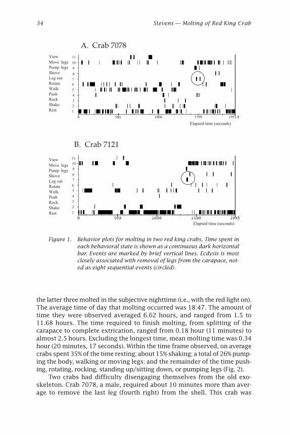
34 Stevens — Molting of Red King Crab
Figure 1. Behavior plots for molting in two red king crabs. Time spent ineach behavioral state is shown as a continuous dark horizontalbar. Events are marked by brief vertical lines. Ecdysis is mostclosely associated with removal of legs from the carapace, not-ed as eight sequential events (circled).
the latter three molted in the subjective nighttime (i.e., with the red light on).The average time of day that molting occurred was 18:47. The amount oftime they were observed averaged 6.62 hours, and ranged from 1.5 to11.68 hours. The time required to finish molting, from splitting of thecarapace to complete extrication, ranged from 0.18 hour (11 minutes) toalmost 2.5 hours. Excluding the longest time, mean molting time was 0.34hour (20 minutes, 17 seconds). Within the time frame observed, on averagecrabs spent 35% of the time resting; about 15% shaking; a total of 26% pump-ing the body, walking or moving legs; and the remainder of the time push-ing, rotating, rocking, standing up/sitting down, or pumping legs (Fig. 2).
Two crabs had difficulty disengaging themselves from the old exo-skeleton. Crab 7078, a male, required about 10 minutes more than aver-age to remove the last leg (fourth right) from the shell. This crab was
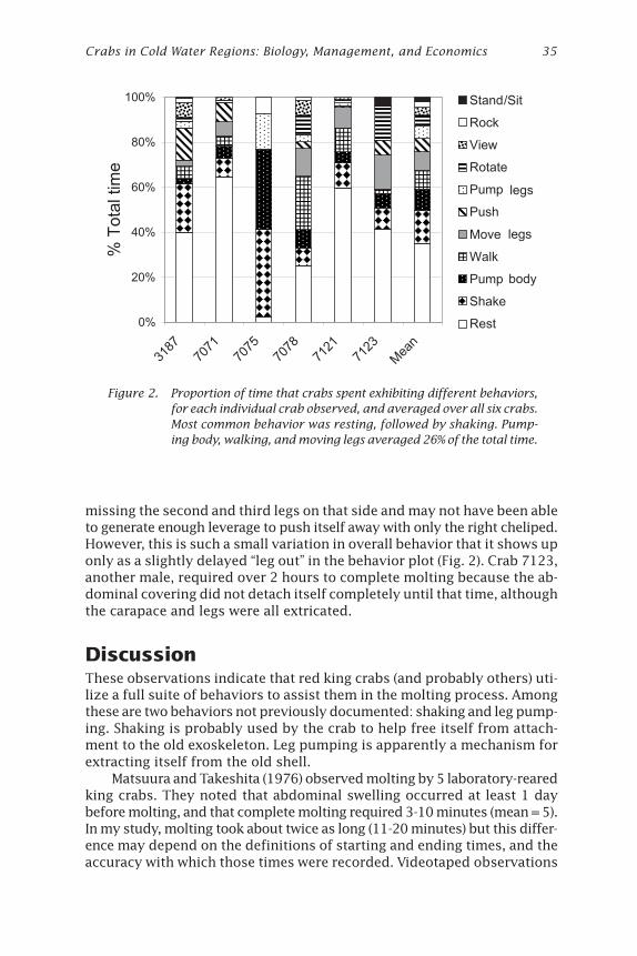
Crabs in Cold Water Regions: Biology, Management, and Economics 35
missing the second and third legs on that side and may not have been ableto generate enough leverage to push itself away with only the right cheliped.However, this is such a small variation in overall behavior that it shows uponly as a slightly delayed “leg out” in the behavior plot (Fig. 2). Crab 7123,another male, required over 2 hours to complete molting because the ab-dominal covering did not detach itself completely until that time, althoughthe carapace and legs were all extricated.
DiscussionThese observations indicate that red king crabs (and probably others) uti-lize a full suite of behaviors to assist them in the molting process. Amongthese are two behaviors not previously documented: shaking and leg pump-ing. Shaking is probably used by the crab to help free itself from attach-ment to the old exoskeleton. Leg pumping is apparently a mechanism forextracting itself from the old shell.
Matsuura and Takeshita (1976) observed molting by 5 laboratory-rearedking crabs. They noted that abdominal swelling occurred at least 1 daybefore molting, and that complete molting required 3-10 minutes (mean = 5).In my study, molting took about twice as long (11-20 minutes) but this differ-ence may depend on the definitions of starting and ending times, and theaccuracy with which those times were recorded. Videotaped observations
Figure 2. Proportion of time that crabs spent exhibiting different behaviors,for each individual crab observed, and averaged over all six crabs.Most common behavior was resting, followed by shaking. Pump-ing body, walking, and moving legs averaged 26% of the total time.
36 Stevens — Molting of Red King Crab
are more accurate because the observer does not have to look away torecord the time of an event, and the videotape can be reviewed for accuracy.
Molting of crustaceans is under hormonal control but may be entrainedto synchronize with an external environmental cue. Molting of larval Ameri-can lobsters (Homarus americanus) to the postlarval stage is synchronizedwith the light:dark cycle; it generally occurs within 10 hours after theonset of darkness whether in a natural or reversed daylight cycle, regard-less of scotophase length (Waddy and Aiken 1999). Molting becomes asyn-chronous within 3 days after exposure to constant light or darkness, andcan be reinstated stepwise over 4 days. Molt timing of American lobstersis also dependent on temperature; molting occurs earlier in the seasonwhen water temperatures are warmer (Tremblay and Eagles 1997). Molt-ing in the shore crab (Carcinus maenas) is circatidal; adult females col-lected from mating pairs during low tide molted at the expected time ofhigh tides in the laboratory (Abello et al. 1997), and wild-caught glaucothoemolted to the first crab stage at times of expected high tide (Zeng et al.1997).
In this study, half (3 of 6) of the crabs molted during daytime, and halfin the subjective nighttime. This sample size is not large enough to makea general statement about the time of molting. Although crabs were ex-posed to a L:D cycle of about 10:14 (from artificial lighting in the labora-tory, longer than available daylight in January) prior to observation, whetherthey retain their entrained natural rhythm after several months in thelaboratory is unknown.
In the confined environment of a laboratory tank, molting crabs usu-ally move away from others, but are often cannibalized soon after molting(personal observation). If loss of legs increases the time required to extri-cate itself from the old shell, such crabs may be more vulnerable to canni-balism or predation during this extended period of vulnerability. In thecase of crab 7078, its vulnerable period (30 minutes) was 50% longer thanaverage (20 minutes). Leg loss is a common effect of the sorting and dis-card process in commercial fisheries (Stevens 1990, MacIntosh et al. 1996);thus, one previously unrecognized effect of handling-induced leg loss ispotentially increased vulnerability to predation during subsequent molts.
Reference to trade names in this paper does not imply endorsementby the National Marine Fisheries Service.
ReferencesAbello, P., C.G. Warman, and E. Naylor. 1997. Circatidal moulting rhythm in the
shore crab Carcinus maenus. J. Mar. Biol. Assoc. U.K. 77:277-280.
Drach, P. 1939. Mue et cycle d’intermue chez les Crustaces Decapodes. Ann. Inst.Oceanogr. 19:103-391.
Crabs in Cold Water Regions: Biology, Management, and Economics 37
MacIntosh, R.A., B.G. Stevens, J.A. Haaga, and B.A. Johnson. 1996. Effects of han-dling and discarding on mortality of Tanner crabs (Chionoecetes bairdi). In:High latitude crabs: Biology, management, and economics. University of Alas-ka Sea Grant, AK-SG-96-02, Fairbanks, pp. 577-590.
Matsuura, S., and K. Takeshita. 1976. Molting and growth of the laboratory-rearedking crab, Paralithodes camtschatica (Tilesius). Rep. Fish. Res. Lab., KyushuUniv. 3:1-14.
Skinner, D.M. 1962. The structure and metabolism of a crustacean integumentarytissue during a molt cycle. Biol. Bull. 123:635-347.
Skinner, D.M. 1985. Molting and regeneration. In: D.E. Bliss (ed.), The biology ofCrustacea. Vol. 9. Integument, pigments, and hormonal processes. AcademicPress, Orlando, Florida, pp. 43-146.
Stevens, B.G. 1990. Survival of king and Tanner crabs captured by commercial soletrawls. Fish. Bull., U.S. 88:731-744.
Tremblay, M.J., and M.D. Eagles. 1997. Molt timing and growth of the lobster, Homar-us americanus, off northeastern Cape Breton Island, Nova Scotia. J. ShellfishRes. 16:383-394.
Waddy, S.L., and D. Aiken. 1999. Timing of the metamorphic molt of the Americanlobster (Homarus americanus) is governed by a population-based, photoperi-odically entrained daily rhythm. Can. J. Fish. Aquat. Sci. 56:2324-2330.
Zeng, C., E. Naylor, and P. Abello. 1997. Endogenous control of timing of metamor-phosis in megalopae of the shore crab Carcinus maenas. Mar. Biol. 128:299-305.
Zhou, S., T.C. Shirley, and G.H. Kruse. 1998. Feeding and growth of the red kingcrab Paralithodes camtschaticus under laboratory conditions. J. Crust. Biol.18:337-345.

Crabs in Cold Water Regions: Biology, Management, and Economics 39Alaska Sea Grant College Program • AK-SG-02-01, 2002
Growth of Red King Crabs fromthe Central Aleutian Islands, AlaskaIvan Vining, S. Forrest Blau, and Douglas PengillyAlaska Department of Fish and Game, Kodiak, Alaska
AbstractGrowth per molt and molting probability were estimated from male redking crabs Paralithodes camtschaticus that were tagged and released duringthe 1970s by Alaska Department of Fish and Game (ADFG) biologists in theAdak Island to Amlia Island area within the Adak (Aleutians) ManagementArea, Alaska. There were 14,742 tagged crabs released, of which 1,385 wererecovered by fishermen during commercial red king crab fisheries, and bysubsequent pot surveys by ADFG. Measurement error and growth per moltin carapace length (CL) were estimated using mixture model analyses. Crabstagged and released in different years had different growth rates, from anaverage growth of approximately 8 mm CL to 16 mm CL in a single year. Themolting probability also varied between years, though high molting prob-abilities were estimated for crabs less than 115 mm CL, and low moltingprobabilities were estimated for crabs greater than 155 mm CL, for all years.
IntroductionAccurate life history information is necessary for proper management ofcommercial marine fisheries. Knowledge of various aspects of growth,such as size at age and annual growth rate, is some of the most importantinformation desired (Powell 1967). Growth parameters have become espe-cially important with increased use of catch-based models (i.e., catch-at-age and catch-at-length models) to estimate population size and trends(Zheng et al. 1995, Collie and Kruse 1998).
Past studies and analyses of growth per molt in king crabs have notinvestigated annual growth variability and used graphical methods tospecify growth. Most of the growth per molt and molting probability analy-ses have been conducted by combining several mark-recapture surveys ora single survey. Moreover, measurement error has only been subjectivelydistinguished from true growth in past studies (Weber and Miyahara 1962,Powell 1967, Weber 1974).
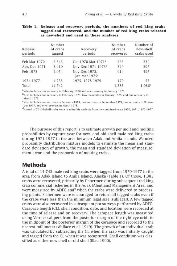
40 Vining et al. — Growth of Red King Crabs
The purpose of this report is to estimate growth per molt and moltingprobabilities by capture year for new- and old-shell male red king crabsduring 1971-1977 in the area between Adak and Amlia islands. We usedprobability distribution mixture models to estimate the mean and stan-dard deviation of growth, the mean and standard deviation of measure-ment error, and the proportion of molting crabs.
MethodsA total of 14,742 male red king crabs were tagged from 1970-1977 in thearea from Adak Island to Amlia Island, Alaska (Table 1). Of those, 1,385crabs were recovered, primarily by fishermen during subsequent red kingcrab commercial fisheries in the Adak (Aleutians) Management Area, andwere measured by ADFG staff when the crabs were delivered to process-ing plants. Fishermen were encouraged to return all tagged crabs even ifthe crabs were less than the minimum legal size (sublegal). A few taggedcrabs were also recovered in subsequent pot surveys performed by ADFG.Carapace length (CL), shell condition, date, and location were recorded atthe time of release and on recovery. The carapace length was measuredusing Vernier calipers from the posterior margin of the right eye orbit tothe midpoint of the posterior margin of the carapace and recorded to thenearest millimeter (Wallace et al. 1949). The growth of an individual crabwas calculated by subtracting the CL when the crab was initially caughtand tagged from the CL when it was recaptured. Shell condition was clas-sified as either new-shell or old-shell (Blau 1990).
Table 1. Release and recovery periods, the numbers of red king crabstagged and recovered, and the number of red king crabs releasedas new-shell and used in these analyses.
Number Number Number ofRelease of crabs Recovery of crabs new-shellperiods tagged periods recovered crabs used
Feb-Mar 1970 2,543 Oct 1970-Mar 1971a 263 239
Apr, Dec 1971 3,410 Nov-Dec 1971-1973b 329 297
Feb 1973 4,054 Nov-Dec 1973, 614 497 Jan-Mar 1975c
1974-1977 4,735 1975, 1978-1979 179 53
Total 14,742 1,385 1,086d
a Also includes one recovery in February 1970 and one recovery in January 1973.bAlso includes one recovery in February 1973, two recoveries in January 1975, and one recovery in March 1975.c Also includes one recovery in February 1974, one recovery in September 1974, one recovery in Novem- ber 1977, and one recovery in March 1978.dA total of 70 old-shell crabs were used in this analysis from the combined years 1970, 1971, 1973-1977.
Crabs in Cold Water Regions: Biology, Management, and Economics 41
The data from recovered male crabs were divided into five samplesfor analysis based on shell condition at release and year of release (Table1). Crabs were separated by shell condition because past studies indicatenew- and old-shell red king crabs have different growth rates and moltingprobabilities (Weber and Miyahara 1962, McCaughran and Powell 1977,Schmidt and Pengilly 1990, Zheng et al. 1995). The recovery of taggedmales released in new-shell condition in each of 1970, 1971, and 1973provided sample sizes sufficient to analyze separately by year of release.However, due to the low number of tag recoveries of crabs tagged andreleased in new-shell condition during 1974-1977 these data were pooledfor analyses, as were the data from males tagged and released in old-shellcondition during 1970, 1971, and 1973-1977. Due to the larger samplesizes, we concentrated our investigation more on the crabs released innew-shell condition during 1970, 1971, and 1973.
Growth per molt was calculated by estimating the parameters of amixture model. A mixture model is a composite of two or more probabil-ity distributions. We estimated a composite of two or more normal distri-butions, with the mean of each normal distribution representing theexpected growth per molt. The formula for a mixture model representinga composite of three normal distributions is:
f x( ) ( , ) ( , ) ( ) ( , )= p m + p m + - p - p m1 1 1 1 2 2 2 2 1 2 3 3 31F F Fs s s
whereF(m, s) = a normal density function with mean m and standard devia-
tion s,
p1 = weight given to F1,
m1 = mean of normal density function F1,
s1 = standard deviation of normal density function F1,
p2 = weight given to F2,
m2 = mean of normal density function F2,
s2 = standard deviation of normal density function F2,
m3 = mean of normal density function F3, and
s3 = standard deviation of normal density function F3.
The parameters p1, m1, s1, p2, m2, s2, m3, and s3 were estimated in this mix-ture model. The mixture model for a composite of two normal distribu-tions is identical to the three normal distributions mixture model exceptthat only one weight parameter and only two normal distribution param-eters are specified.
In the context of our estimation of growth per molt, F1(m1, s1) repre-sents the distribution of measurement error that can occur at the time oftagging and recovery of crabs that did not molt, and p1 represents theproportion in a sample of recovered crabs that did not molt. The second
42 Vining et al. — Growth of Red King Crabs
and third normal distributions F2(m2, s2) and F3(m3, s3) represent the growthin a single molt and in two molts, respectively, plus independent mea-surement error that can occur at the time of release and recovery. Theweights p2 and (1 – p1 – p2) represent the proportions in a sample of recov-ered crabs that molted and grew one and two times, respectively.
Maximum likelihood estimates of the mixture model were computedby minimizing the negative log likelihood (Venables and Ripley 1994). Thefunctions used to estimate the mixture model parameters were written inthe statistical package/language S-Plus (MathSoft 1998) by Venables andRipley (1994). Parameter standard error calculations were calculated fromthe information matrix generated by the minimization estimate of Venablesand Ripley (1994). Histograms of the growth data were used to provideguidance on the number of normal distributions that were likely present.When more than one model was possible, convergence to a unique solu-tion and comparability of the parameter estimates to published estimatesof red king crab growth were used to evaluate the best model.
The mixture model results were compared to the growth of recoveredcrabs to identify crabs that had not molted (i.e., the apparent “growth”represented measurement error) and crabs that had molted or grown priorto recovery. The male red king crabs that were at large for approximately1 year (8-14 months) and had lived through one “molting season” weregiven a binary attribute “0” if they were classified as not having moltedand “1” if they were identified as having molted and grown.
A logit model was fit to molting probability versus carapace length.The form of the logit model (MathSoft, Inc. 1997) was:
p
ee
x
x=
+
+
+
a b
a b1
wherex = carapace length of a red king crab at release,
p = probability of molting in one year for red king crabs of carapace length x, and
a and b are logit model parameters to be estimated.
A generalized linear model (glm) function in S-Plus (MathSoft 1998) wasemployed to estimate the parameters of the logit model. The carapacelengths where 10%, 50%, and 90% of the crabs will have molted was esti-mated from the logit model.
ResultsScatterplots of apparent growth in carapace length for recovered malesreleased in new-shell condition indicated most of the smaller crabs (<120mm CL) molted at least once, but few large crabs (>155 mm CL) molted.
Crabs in Cold Water Regions: Biology, Management, and Economics 43
Little or no dependency of growth on size at release was evident in thescatterplots.
The mixture model parameters for the crabs released in new-shellcondition during 1970 were estimated using a two-normal-distributionsmodel (Fig. 1a), whereas the mixture model parameters for the crabs re-leased in 1971 and 1973 were each analyzed using a three-normal-distri-butions model (Figs. 1b and 1c). The pooled new-shell and old-shell sampleswere both analyzed using a two-normal-distributions model.
The estimated parameters for the different mixture models varied byyear (Table 2). Estimates of the portion of crabs within a sample that didnot molt ranged from 0.19 for males released as new-shells in 1971 to0.84 for males released as new-shells in 1970. The estimated average growthfrom one molt was similar for crabs released in new-shell condition dur-ing 1970 (10.6 mm CL) and during 1973 (10.8 mm CL). The estimatedaverage growth from a single molt for crabs released in new-shell condi-tion during 1971 was 15.7 mm CL, indicating a possibly higher growth ofmolting crabs between 1971 and 1972 than during the other molting sea-sons. The average growth from a single molt estimated from the poolednew- and old-shell samples was considerably lower (8.3 mm and 8.8 mmCL respectively) than the estimates from the other samples. To comparethe growth from one molt between sample years and shell condition, 95%confidence intervals were estimated for the mean of the first growth-per-molt. The 95% confidence interval for new-shell crabs of 1970 was 9.5-11.6 mm, for 1971 it was 15.3-16.1 mm, for 1973 it was 10.1-11.6 mm,and for 1974-1977 it was 6.7-9.9 mm, with old-shell being from 7.3 to 10.4mm. This shows that new-shell growth for the first molt was not signifi-cantly different between 1970 and 1973, but the growth from 1971 wasdifferent. Also, though marginal, the combined new-shell 1974-1977 growthfor the first molt was not significantly different from 1970, but was sig-nificantly different from 1971 and 1973. The old-shell growth for the firstmolt was only significantly different from the 1971 new-shell growth.
Average growth from two molts was estimated as 26.7 mm CL fromthe sample of males released as new-shells in 1971 and 28.0 mm CL fromthe sample of males released as new-shells in 1973 (Table 2). Estimatedmean measurement error for each sample was within 1 standard error of0.0 mm CL, and the standard deviation of measurement error was esti-mated to be less than 1.0 mm CL in each sample (Table 2).
A change in carapace length of ≥5 mm was used as an indication ofgrowth. From the mixture model analysis, the probability that a ≥5 mmchange was due to measurement error was less than 0.001 for all yearsand shell conditions, indicating a difference in carapace length of 5 mm ormore was not due to measurement error. The probability of crabs at re-lease size molting within 8-14 months after release, as estimated by thelogit model, varied among samples (Table 3, Fig. 2). All models indicatedhigh probabilities (>0.9) of molting within 8-14 months for males £118mm CL, and low molting probabilities (<0.1) for males ≥154 mm CL (Table 4).
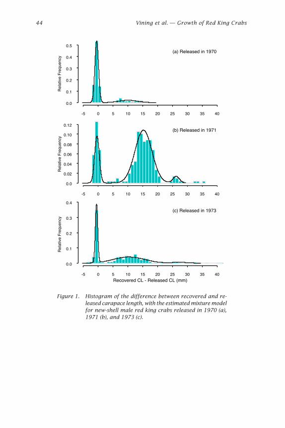
44 Vining et al. — Growth of Red King Crabs
Figure 1. Histogram of the difference between recovered and re-leased carapace length, with the estimated mixture modelfor new-shell male red king crabs released in 1970 (a),1971 (b), and 1973 (c).
0.0
0.1
0.2
0.3
0.4
0.5
Rel
ativ
e F
requ
ency
-5 0 5 10 15 20 25 30 35 40
(a) Released in 1970
0.0
0.02
0.04
0.06
0.08
0.10
0.12
Rel
ativ
e F
requ
ency
-5 0 5 10 15 20 25 30 35 40
(b) Released in 1971
0.0
0.1
0.2
0.3
0.4
Rel
ativ
e F
requ
ency
-5 0 5 10 15 20 25 30 35 40
(c) Released in 1973
Recovered CL - Released CL (mm)
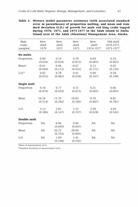
Crabs in Cold Water Regions: Biology, Management, and Economics 45
Table 2. Mixture model parameter estimates (with associated standarderror in parentheses) of proportion molting, and mean and stan-dard deviation (S.D.) of growth for male red king crabs taggedduring 1970, 1971, and 1973-1977 in the Adak Island to AmliaIsland area of the Adak (Aleutians) Management Area, Alaska.
Male New- New- New- New- Old-shell crabs shell shell shell shell 1970,1971,sampled 1970 1971 1973 1974-1977 1973-1977
No molts
Proportion 0.84 0.19 0.39 0.69 0.34(0.024) (0.024) (0.023) (0.065) (0.063)
Meana –0.01 0.08 –0.07 0.13 0.03(0.044) (0.112) (0.033) (0.151) (0.134)
S.D.b 0.62 0.78 0.41 0.90 0.58(0.032) (0.082) (0.030) (0.107) (0.108)
Single molt
Proportion 0.16 0.77 0.55 0.31 0.66(0.024) (0.026) (0.025) (0.065) (0.063)
Mean 10.56 15.70 10.83 8.29 8.81(0.514) (0.202) (0.382) (0.807) (0.781)
S.D. 3.13 2.85 5.35 2.99 4.69(0.386) (0.147) (0.337) (0.628) (0.542)
Double molt
Proportion NA 0.04 0.06 NA NA(0.049) (0.047)
Mean NA 26.72 28.04 NA NA(0.354) (0.893)
S.D. NA 1.09 3.41 NA NA(0.248) (0.592)
aMean of measurement error.bStandard deviation of measurement error.
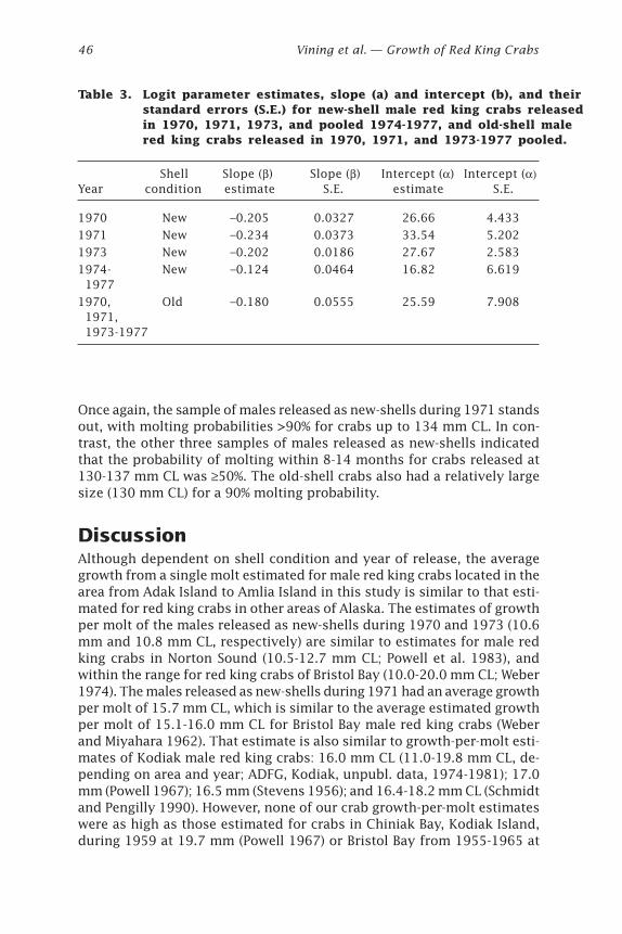
46 Vining et al. — Growth of Red King Crabs
Table 3. Logit parameter estimates, slope (a) and intercept (b), and theirstandard errors (S.E.) for new-shell male red king crabs releasedin 1970, 1971, 1973, and pooled 1974-1977, and old-shell malered king crabs released in 1970, 1971, and 1973-1977 pooled.
Shell Slope (b) Slope (b) Intercept (a) Intercept (a)Year condition estimate S.E. estimate S.E.
1970 New –0.205 0.0327 26.66 4.433
1971 New –0.234 0.0373 33.54 5.202
1973 New –0.202 0.0186 27.67 2.583
1974- New –0.124 0.0464 16.82 6.619 1977
1970, Old –0.180 0.0555 25.59 7.908 1971, 1973-1977
Once again, the sample of males released as new-shells during 1971 standsout, with molting probabilities >90% for crabs up to 134 mm CL. In con-trast, the other three samples of males released as new-shells indicatedthat the probability of molting within 8-14 months for crabs released at130-137 mm CL was ≥50%. The old-shell crabs also had a relatively largesize (130 mm CL) for a 90% molting probability.
DiscussionAlthough dependent on shell condition and year of release, the averagegrowth from a single molt estimated for male red king crabs located in thearea from Adak Island to Amlia Island in this study is similar to that esti-mated for red king crabs in other areas of Alaska. The estimates of growthper molt of the males released as new-shells during 1970 and 1973 (10.6mm and 10.8 mm CL, respectively) are similar to estimates for male redking crabs in Norton Sound (10.5-12.7 mm CL; Powell et al. 1983), andwithin the range for red king crabs of Bristol Bay (10.0-20.0 mm CL; Weber1974). The males released as new-shells during 1971 had an average growthper molt of 15.7 mm CL, which is similar to the average estimated growthper molt of 15.1-16.0 mm CL for Bristol Bay male red king crabs (Weberand Miyahara 1962). That estimate is also similar to growth-per-molt esti-mates of Kodiak male red king crabs: 16.0 mm CL (11.0-19.8 mm CL, de-pending on area and year; ADFG, Kodiak, unpubl. data, 1974-1981); 17.0mm (Powell 1967); 16.5 mm (Stevens 1956); and 16.4-18.2 mm CL (Schmidtand Pengilly 1990). However, none of our crab growth-per-molt estimateswere as high as those estimated for crabs in Chiniak Bay, Kodiak Island,during 1959 at 19.7 mm (Powell 1967) or Bristol Bay from 1955-1965 at
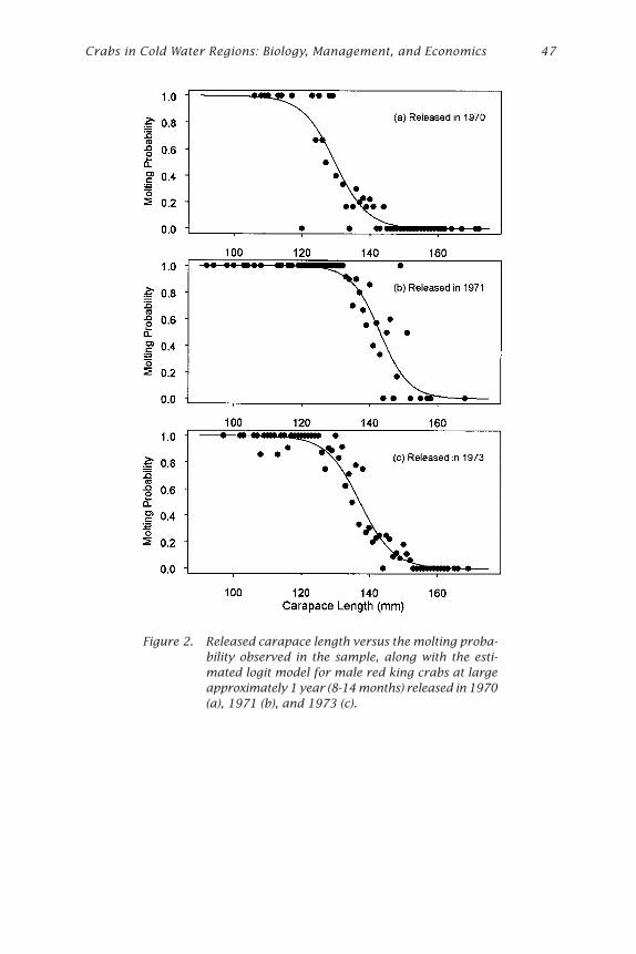
Crabs in Cold Water Regions: Biology, Management, and Economics 47
Figure 2. Released carapace length versus the molting proba-bility observed in the sample, along with the esti-mated logit model for male red king crabs at largeapproximately 1 year (8-14 months) released in 1970(a), 1971 (b), and 1973 (c).
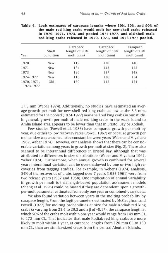
48 Vining et al. — Growth of Red King Crabs
17.5 mm (Weber 1974). Additionally, no studies have estimated an aver-age growth per molt for new-shell red king crabs as low as the 8.3 mm,estimated for the pooled (1974-1977) new-shell red king crabs in our study.In general, growth per molt of male red king crabs in the Adak Island toAmlia Island area appears to be lower than that in Bristol Bay or Kodiak.
Few studies (Powell et al. 1983) have compared growth per molt byyear, due either to low recovery rates (Powell 1967) or because growth permolt at size was assumed to be constant between years (Weber and Miyahara1962, Weber 1974). However, our analysis shows that there can be consid-erable variation among years in growth per molt at size (Fig. 2). There alsoseemed to be interannual differences in Bristol Bay, although that wasattributed to differences in size distributions (Weber and Miyahara 1962,Weber 1974). Furthermore, when annual growth is combined for severalyears interannual variation can be overshadowed by one or two high re-coveries from tagging studies. For example, in Weber’s (1974) analysis,54% of the recoveries of crabs tagged over 7 years (1955-1961) were fromtwo release years (1957 and 1958). One implication of annual variabilityin growth per molt is that length-based population assessment models(Zheng et al. 1995) could be biased if they are dependent upon a growth-per-molt parameter estimated from only one year or combined-years data.
We also found variation between years in the molting probability bycarapace length. From the logit parameters estimated by McCaughran andPowell (1977) for molting probabilities at size for male Kodiak red kingcrabs (a varying from 25.4 to 29.3 and a b of –0.17), the carapace length atwhich 50% of the crabs molt within one year would range from 149 mm CLto 172 mm CL. That indicates that male Kodiak red king crabs are morelikely to molt within 1 year, at carapace lengths from 120 mm CL to 150mm CL, than are similar-sized crabs from the central Aleutian Islands.
Table 4. Logit estimates of carapace lengths where 10%, 50%, and 90% ofthe male red king crabs would molt for new-shell crabs releasedin 1970, 1971, 1973, and pooled 1974-1977, and old-shell malered king crabs released in 1970, 1971, and 1973-1977 pooled.
Carapace Carapace Carapace Shell length of 90% length of 50% length of10%
Year condition molt (mm) molt (mm) molt (mm)
1970 New 119 130 140
1971 New 134 143 152
1973 New 126 137 148
1974-1977 New 118 136 154
1970, 1971, Old 130 142 154 1973-1977
Crabs in Cold Water Regions: Biology, Management, and Economics 49
Both the growth per molt and molting probability estimates couldhave been influenced by recapture bias because most tag recoveries werecollected by the fishing fleet. Sublegal crabs may have been recoveredless often than legal-sized crabs. Hence, growth of males released assublegals may be over-represented because if a sublegal crab did not molt,thus retaining its sublegal classification, it was less likely to be reportedsince it would not be legal to keep under normal circumstances. However,the tagging studies that provided growth-per-molt estimates of male redking crabs in other areas of Alaska also relied upon king crab commercialfisheries for tag recoveries.
Differences between years observed in the growth per molt and molt-ing probabilities in the Adak Island to Amlia Island area could be due tochanges in environmental conditions or spatial variability. Favorable en-vironmental conditions could likely lead to greater growth and highermolting probabilities. However, we have found no data to indicate anymajor difference in temperature or other environmental conditions. Thesamples collected in the Adak Island to Amlia Island area were all from thesame general area (Blau 1993), so any differences were not likely due tospatial differences.
Finally, we note the utility of mixture models in estimating growth-per-molt parameters of crabs. The value of the mixture-model approach isthat it allows for estimating parameters of measurement error and growthfrom one or more molts without any a priori specification of the range ofvalues that represent no molts (measurement error), one molt, or multiplemolts.
AcknowledgmentsSpecial thanks are due to all ADFG staff, fishermen, and seafood proces-sors who were involved with the tag and recovery efforts on Adak red kingcrabs over the years. Specifically the primary ADFG shellfish biologists incharge of the various Adak red king crab surveys in the 1970s included: K.Griffin, C. Hurd, R. Nelson, J. McMullen, A. Schmidt, R. Tamburelli, P. Tate,and H. Yoshihara. G. Powell planned the 1975-1977 surveys. S. Harris en-tered all the data. This is contribution PP-205 of the Alaska Department ofFish and Game, Commercial Fisheries Division, Juneau.
ReferencesBlau, S.F. 1990. Size at maturity of female red king crabs (Paralithodes camtschati-
ca) in the Adak Management Area, Alaska. In: Proceedings of the InternationalSymposium on King and Tanner Crabs. University of Alaska Sea Grant, AK-SG-90-04, Fairbanks, pp. 105-116.
50 Vining et al. — Growth of Red King Crabs
Blau, S.F. 1993. Overview of the red king crab surveys conducted in the Adak Manage-ment Area R, Alaska, 1969-87. Alaska Department of Fish and Game, Division ofCommercial Fisheries, Regional Information Report 4K93-10, Kodiak. 42 pp.
Collie, J.S., and G.H. Kruse. 1998. Estimating king crab (Paralithodes camtchaticus)abundance from commercial catch and research survey data. In: G.S. Jamiesonand A. Campbell (eds.), Proceedings of the North Pacific Symposium on Inver-tebrate Stock Assessment and Management. Can. Spec. Publ. Fish. Aquat. Sci.125:73-83.
MathSoft, Inc. 1997. S-Plus 4.0, guide to statistics. Data Analysis Products Division,MathSoft, Seattle. 877 pp.
MathSoft, Inc. 1998. S-Plus 4.5, release 2. MathSoft, Seattle.
McCaughran, D.A., and G.C. Powell. 1977. Growth model for Alaska king crab(Paralithodes camtschatica). J. Fish. Res. Board Can. 34:989-995.
Powell, G.C. 1967. Growth of king crabs in the vicinity of Kodiak Island, Alaska.Alaska Department of Fish and Game, Informational Leaflet 6, Juneau. 106 pp.
Powell, G.C., R. Peterson, and L. Schwarz. 1983. The red king crab, Paralithodescamtschatica (Tilesius) in Norton Sound, Alaska: History of biological researchand resource utilization through 1982. Alaska Department of Fish and Game,Information Leaflet 222, Juneau. 104 pp.
Schmidt, D., and D. Pengilly. 1990. Alternative red king crab fishery managementpractices: Modeling the effects of varying size-sex restrictions and harvestrates. In: Proceedings of the International Symposium on King and TannerCrabs. University of Alaska Sea Grant, AK-SG-90-04, Fairbanks, pp. 551-566.
Stevens, H.R. 1956. Progress report on king crab research. Alaska Department ofFisheries, Annual Report for 1955. Alaska Fisheries Board and Alaska Depart-ment of Fisheries Rep. 7:87-93.
Venables, W.N., and B.D. Ripley. 1994. Modern applied statistics with S-Plus. Springer-Verlag, New York. 462 pp.
Wallace, M.M., C.J. Pertuit, and A.R. Hvatum. 1949. Contribution to the biology ofking crab (Paralithodes camtschatica Tilesius). U.S. Fish Wildl. Serv., Fish. Leaf-let 340. 50 pp.
Weber, D.D. 1974. Observation on growth of southeastern Bering Sea king crab,Paralithodes camtschatica, from a tag-recovery study, 1955-65. NMFS-DR-86,Seattle. 122 pp.
Weber, D.D., and T. Miyahara. 1962. Growth of the adult king crab Paralithodescamtschatica (Tilesius). Fish. Bull., U.S. 62:53-75.
Zheng, J., M.C. Murphy, and G.H. Kruse. 1995. A length-based population modeland stock-recruitment relationships for red king crab, Paralithodes camtschat-icus, in Bristol Bay, Alaska. Can. J. Fish. Aquat. Sci. 52:1229-1246.
Crabs in Cold Water Regions: Biology, Management, and Economics 51Alaska Sea Grant College Program • AK-SG-02-01, 2002
Estimating Natural Mortalityof King Crabs from TagRecapture DataM.S.M. SiddeekAlaska Department of Fish and Game, Commercial Fisheries Division,Juneau, Alaska
Leslie J. Watson and S. Forrest BlauAlaska Department of Fish and Game, Commercial Fisheries Division,Kodiak, Alaska
Holly MooreAlaska Department of Fish and Game, Commercial Fisheries Division,Dutch Harbor, Alaska
AbstractNatural mortality (M) is used as a surrogate for the maximum sustainableyield level of fishing mortality in determining limit and target referencepoints under precautionary management for the Bering Sea and AleutianIslands (BSAI) crab stocks. Precise M estimates are needed to improve stock-assessment models as well as computer-simulation models for evaluatingalternative harvest strategies. In the federal crab fishery management planfor the BSAI areas, an annual M of 0.3 for Tanner and snow crabs(Chionoecetes) and 0.2 for king crabs (Lithodes and Paralithodes) wereadopted. We attempted to determine plausible M values for BSAI golden,red, and blue king crab stocks by employing an optimization routine thatminimized the differences between observed and expected effective taggedpopulations based on 1990s tag-release-recapture data. The age-based-Virtual Population Analysis (VPA) M estimator produced an annual M of0.38 for male golden king crabs in the Aleutian Islands and 0.54 for malered king crabs in Bristol Bay. The annual M estimated by the multinomialmaximum likelihood method for St. Matthew Island combined sexes blueking crabs was 0.19. The length-based-VPA M estimator was annually vari-able and ranged from 0.02 to 1.62 for the Bristol Bay red king crab males.The red king crabs M estimates appeared high considering its longevity.
52 Siddeek et al. — Estimating Natural Mortality
The simplified assumptions made for the length-based analysis cast doubton the variable M estimates. Type A error was high among all experiments,but was estimated from the models and hence did not affect M estimates.
IntroductionThe instantaneous natural mortality (M ) is an important parameter in BeringSea and Aleutian Islands (BSAI) crab stock assessment and management(NPFMC 1999). The analysis and data are poor for most BSAI crab stocks;consequently, M is used as a surrogate for the maximum sustainable yieldlevel of fishing mortality (FMSY) in determining limit and target referencepoints under precautionary management (Restrepo et al. 1998).
Although M of BSAI crabs is likely to vary by size, age (Hirschhorn1966, Balsiger 1974, Reeves and Marasco 1980, Reeves 1988, Greenberget al. 1991), or year (Zheng et al. 1995a), finding a constant or average Mreflecting the longevity of the species is directly relevant to current crabstock assessment and management, and helps to obtain a direct estimateof FMSY. Although M may not frequently equal FMSY, one could establish arelationship between F and M to obtain an optimum yield (Siddeek, ADFG,unpubl.). Thus, estimation of M appears to be a useful exercise, althougha difficult one, for heavily exploited stocks such as BSAI crabs. Therefore,in this paper we attempted to estimate M for Aleutian Islands golden kingcrab (Lithodes aequispinus), Bristol Bay red king crab (Paralithodescamtschaticus), and St. Matthew Island blue king crab (P. platypus) usingtag-recapture data with a suite of optimization techniques.
Tag-recapture data have been used in the past to estimate M and manyother parameters of BSAI crab stocks. Hirschhorn (1966) and Balsiger (1974)used data from the 1950s and 1960s tag-recaptures with effort data toestimate size-specific annual M for Bristol Bay red king crab males in thesize range 80-179 mm carapace length (CL). The estimates varied from0.001 to 0.93 for the size range 80-169 mm CL with M increasing by size(Balsiger 1974). Other size-specific M estimates based on trawl survey dataranged from 0.08 to 1.21 for the size range 85-169 mm CL, but smallercrabs (<125 mm CL) had higher natural mortality (Reeves and Marasco1980, Reeves 1988, Greenberg et al. 1991, Zheng et al. 1995a). Zheng et al.(1995a) reviewed those estimates and concluded that a curve of M mightbe bowl-shaped when plotted by length and varied over time. Althoughsound statistical methodologies have been employed in a number of tag-recapture and trawl-survey data analyses (e.g., Balsiger 1974), they sufferfrom the confounding effect of both M and the catchability coefficient (q)in the estimation process. Siddeek (1989, 1991) developed an optimiza-tion technique based on Pope’s (1972) cohort (or virtual population analy-sis, VPA) formulas for estimating M using tag-recapture data, obtainedunder either variable or constant intervening F without fishing effort. Weadopted this method in this paper to reduce the confounding error on Mestimation. We formulated a new length-based VPA M estimator following
Crabs in Cold Water Regions: Biology, Management, and Economics 53
Zheng et al.’s (1995a) length-based model for crab populations. We alsoapplied the multinomial maximum likelihood estimator (Seber 1982, Hamp-ton 2000) to experiments for which a VPA M estimator could not be ap-plied. We used the 1990s tag-recapture data to assess the natural mortalitypattern in recent years.
Materials and MethodsTag ReleasesThe Alaska Department of Fish and Game (ADFG) conducted tagging sur-veys of Bristol Bay red king crabs in 1990, 1991, and 1993 (Watson 1992,Pengilly and Watson 1992, Watson and Pengilly 1994); St. Matthew Islandblue king crabs in 1995 and 1998 (Blau 1996, Blau and Watson 1999); andAleutian Islands golden king crabs in 1991 and 1997 (Blau and Pengilly1994, Blau et al. 1998) by chartered commercial crab vessels (Table 1).(Adak and Dutch Harbor areas were combined and are now Aleutian Is-lands.) These tagging experiments were conducted during summer monthsbefore the fishing season started. Recaptures were used for refinement oftrawl survey population size estimates, estimation of exploitation rates,establishment of relative population indexes, and estimation of growthand mortality parameters.
Rectangular, king crab pots were used to capture crabs for tagging inall surveys with the exception of the 1991 golden king crab survey in theAleutian Islands where smaller, conical pots were used. Tagging location,date, and fishing depth were recorded for each pot retrieved. Upon potretrieval, carapace length of crabs was measured to the nearest millime-ter, shell condition recorded, tagged, and released on or adjacent to thecapture location. Isthmus-loop tags (spaghetti or Floy tags) were used totag crabs (Gray 1965) larger than 80-90 mm CL. Internal, passive inte-grated transponder (PIT) tags were also used on some legal-sized (>152.4-mm carapace width (CW)) blue king crabs during the 1995 St. MatthewIsland survey, but recovery rates were so poor that data were excludedfrom current analysis (Blau 1996). The carapace length of each crab wasmeasured from the posterior margin of the right eye orbit to the midpointof the posterior margin of the carapace with Vernier calipers (Wallace et al.1949). The exoskeletal condition on each crab was categorized either asnew-shell (1), old-shell (2), or very old-shell (3) based primarily on thedegree of scratching on the coxae (Wallace et al. 1949). Sublegal or legalsize for males was determined by measuring carapace width (the straight-line distance across the carapace, including the adjacent outer spines)using fixed measuring sticks set at 5.5 inches (139.7 mm CW) for blue kingcrabs, 6.0 inches (152.4 mm CW) for golden king crabs, and 6.5 inches(165.1-mm CW) for red king crabs. Tag recoveries were recorded by onboardobservers at sea and by ADFG dockside samplers at various crab process-ing plants.
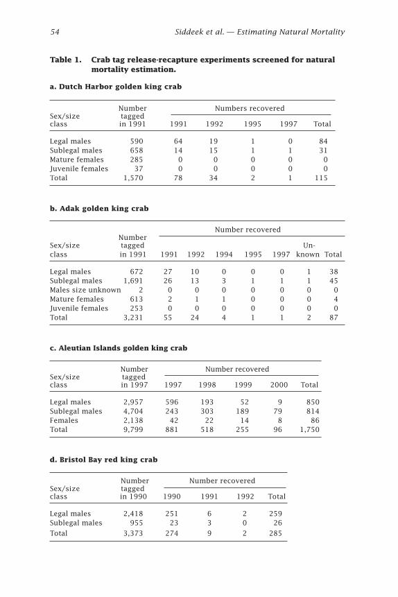
54 Siddeek et al. — Estimating Natural Mortality
Table 1. Crab tag release-recapture experiments screened for naturalmortality estimation.
a. Dutch Harbor golden king crab
Number Numbers recoveredSex/size taggedclass in 1991 1991 1992 1995 1997 Total
Legal males 590 64 19 1 0 84Sublegal males 658 14 15 1 1 31Mature females 285 0 0 0 0 0Juvenile females 37 0 0 0 0 0Total 1,570 78 34 2 1 115
b. Adak golden king crab
Number recovered Number
Sex/size tagged Un-class in 1991 1991 1992 1994 1995 1997 known Total
Legal males 672 27 10 0 0 0 1 38Sublegal males 1,691 26 13 3 1 1 1 45Males size unknown 2 0 0 0 0 0 0 0Mature females 613 2 1 1 0 0 0 4Juvenile females 253 0 0 0 0 0 0 0Total 3,231 55 24 4 1 1 2 87
c. Aleutian Islands golden king crab
Number Number recoveredSex/size taggedclass in 1997 1997 1998 1999 2000 Total
Legal males 2,957 596 193 52 9 850Sublegal males 4,704 243 303 189 79 814Females 2,138 42 22 14 8 86Total 9,799 881 518 255 96 1,750
d. Bristol Bay red king crab
Number Number recoveredSex/size taggedclass in 1990 1990 1991 1992 Total
Legal males 2,418 251 6 2 259Sublegal males 955 23 3 0 26
Total 3,373 274 9 2 285
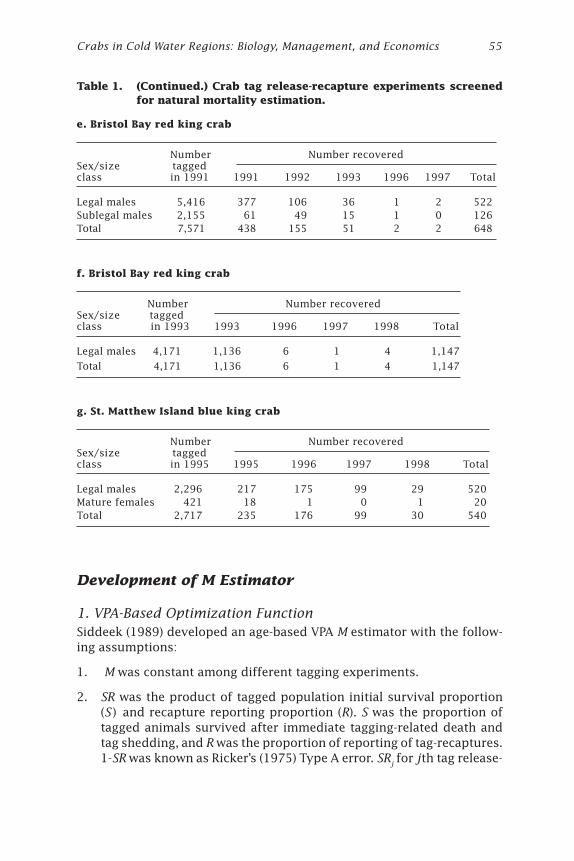
Crabs in Cold Water Regions: Biology, Management, and Economics 55
Table 1. (Continued.) Crab tag release-recapture experiments screenedfor natural mortality estimation.
Development of M Estimator
1. VPA-Based Optimization FunctionSiddeek (1989) developed an age-based VPA M estimator with the follow-ing assumptions:
1. M was constant among different tagging experiments.
2. SR was the product of tagged population initial survival proportion(S ) and recapture reporting proportion (R). S was the proportion oftagged animals survived after immediate tagging-related death andtag shedding, and R was the proportion of reporting of tag-recaptures.1-SR was known as Ricker’s (1975) Type A error. SRj for jth tag release-
e. Bristol Bay red king crab
Number Number recoveredSex/size taggedclass in 1991 1991 1992 1993 1996 1997 Total
Legal males 5,416 377 106 36 1 2 522Sublegal males 2,155 61 49 15 1 0 126Total 7,571 438 155 51 2 2 648
f. Bristol Bay red king crab
Number Number recoveredSex/size taggedclass in 1993 1993 1996 1997 1998 Total
Legal males 4,171 1,136 6 1 4 1,147
Total 4,171 1,136 6 1 4 1,147
g. St. Matthew Island blue king crab
Number Number recoveredSex/size taggedclass in 1995 1995 1996 1997 1998 Total
Legal males 2,296 217 175 99 29 520Mature females 421 18 1 0 1 20Total 2,717 235 176 99 30 540
56 Siddeek et al. — Estimating Natural Mortality
recapture experiment (hereafter referred to as experiment) was nor-mally distributed with a common mean and standard deviation.
3. Two groups of experiments considered for optimization had suffereddifferent magnitudes of annual instantaneous total mortality (Z ).
4. Numerous releases were made in each experiment to conform to de-terministic mortality process and to minimize dependence betweensuccessive recaptures.
We modified some of the above assumptions to suit the current tag-recapture data analysis as follows:
1. SRj for jth experiment within a group of experiments was distributedlog normally with a common mean and standard deviation. Comparedto commercial catches, tag recaptures were few and lognormal errorstructure reduced heteroscedasticity of SR variance.
The assumption of a common mean ln(SR) for a selected group ofexperiments is plausible because we chose the group members to havethe same species, season of tagging, type of tag, and condition ofhandling. Furthermore, we arbitrarily grouped the experiments by tri-al estimated closer SRj values.
2. At least two experiments with different magnitudes of Z were avail-able. Although one experiment would be sufficient to determine Mfrom the minimization functions 7 and 16 developed in the subse-quent sections, nevertheless, following Silliman’s [1943] approach ofsolving two simultaneous equations with varying total mortality andeffort for a unique M solution, we used at least two experiments withdifferent Z (hence different F ) values in the minimization functionsfor M estimation.
The SRj for jth experiment was estimated by the following steps:
N N e C ejt jtM
jty Mj
+- - -= -1
1( ) (1)
and
N N e C ejt jtM
jty Mj= ++1
(2)
whereNjt+1 = tagged population number from jth experiment at the start of
t+1th time period (duration of a time period was set to one year) after release,
Cjt = observed number of tag recaptures from jth experiment during tth time period after release,
Crabs in Cold Water Regions: Biology, Management, and Economics 57
M = constant annual instantaneous natural mortality of the taggedpopulation during tth time period after release, and
yj = time fraction in years from the mid-date of jth tag releases to mid-or start date of the first fishing season.
Following Pope (1972),
SR
NC e C e C e N ej
jj
y Mj
y M Mjt
yjn
nMj j jM tM= + + + + ++ +1
00 1[ ... ... ] (3)
Njn was estimated using the following relation:
N
C Z
F ejnjn n
nZn
=- -( )1
(4)
whereZn = annual instantaneous total mortality of the tagged population
during the last tag recovery time period after release, n, and
Fn = annual instantaneous fishing mortality of the tagged population during the last tag recovery time period after release, n.
The Zn (and hence Fn by subtracting a given M value from Zn) to tunethe VPA to estimate SRj for jth experiment was determined by fitting alinear regression to the natural log of the Baranov’s catch equation (i.e.,modified from equation [18] with constant F, M, Z, yj, and d) as follows:
ln( ) ln[( / )( )]C F SR N Z e My tZjt j jZ
j+-+ = ¥ ¥ - - -1 01 1 d (5)
whereln = natural logarithm.
The minimization function (7) to estimate M from observed tag recap-ture data (Cjt
) was formulated by the following steps:
SR Sjj= Ree (6)
whereSRj = estimated product of initial survival and reporting proportions
for jth experiment, and
ej = a normal random error with a mean of zero and standard devia-tion s,
ln(SR) = expected (mean) value of ln(SRj); and
58 Siddeek et al. — Estimating Natural Mortality
[ln( ) ln( )]SR SRjjk -Â =
21
(7)
wherek = number of experiments in the selected group.
We opted to formulate the minimization function based on SRj ratherthan Cjt because errors in Njt (and hence SRj) estimates shrink during thebackward computation process as the number of time steps of calculationincreases (Pope 1972). Ln(SRj) and ln(SR) can be considered as a form ofobserved and expected ln(SR). Note that SRj has the accumulation of allobserved catches and similarly we may think of SR to have the accumula-tion of all expected catches.
The above was an age-based approach, which could be extended to alength-based form used in crab population modeling. Following Sullivanet al. (1990) and Zheng et al. (1995a),
[ ] [ ][ ][ ]N P m Al t l l t l tji ji l ji ji+ ¢=1 (8)
where[ ] = matrix sign,
A N O e C el t l t l t
Ml t
y M
ji ji jit
ji
j t= + -- - -( ) ( )1 (9)
Nljit = new-shell tagged populations of length class lji in jth experiment during the tth time period after release,
Cljit = number of tag recoveries of length class lji in jth experiment during the tth time period after release,
Oljit = old-shell tagged populations of length class lji in jth experiment during the tth time period after release,
O N O e C e ml t l t l t
Ml t
y Ml tji ji ji
tji
j t
ji= + - -- - -[( ) ]( )( )1 1 , (10)
mljit = molting probability of crabs in length class lji in jth experiment during the tth time period after release,
Mt = annually variable instantaneous natural mortality of crabs in length class lji in jth experiment during the tth time period after release, and
Pljil ¢
= probability of crabs in length class lji in jth experiment growing to length class l ¢¢ The annual growth increment (x) was assumed to have a gamma distribution as follows:
Crabs in Cold Water Regions: Biology, Management, and Economics 59
P
gamma x dx
gamma x dx
l l
ll
l
ll
l
i
nji
jil ji
l ji
jil ji
l jij¢
¢ -
¢ -
¢ -
¢ -
=
=
Ú
ÚÂ
( / , )
( / , )
a b
a b
t
t
t
t
1
2
1
2
1
(11)
gamma x
x el
x
l jiji
l ji
l ji( / , )
( )a b
b a
a b
a=- -1
G, (12)
wherenj = number of length classes in the jth experiment,
l¢1 and l¢2 = lower and upper limits, respectively, of the receiving length class l¢,
b = a parameter of the gamma distribution,
a bl lji ji
G= / , and (13)
Glji = mean annual growth increment per molt for the length class lji in jth experiment with a middle carapace length tlji just before molting.
The mean annual growth increment was assumed to be a linear functionof the molting class mid-length as follows:
G a bl ji l ji
= + t , (14)
wherea and b = constants.
We assumed Mt to be length invariant for the current tag-recaptureanalysis. For simplicity, we also assumed all recaptures were new shells.Therefore, the term Oljit in equation 9 and the entire equation 10 wereignored in the current analysis. See the discussion section for justification.
The terminal population abundance vector Nljin for experiment j wasestimated using equation 4 for each size group i with a constant Zn esti-mated from equation 5 and Fn calculated from Zn by subtracting a given Mvalue. This population size vector was projected backward by one step byinverse matrix multiplication to obtain the previous time-step populationsize vector as follows:
[ ] [ ] [ ] [ ] [ ]N m P N e C el t l t l l l t
Ml t
y M
ji ji ji ji ji
j= +-¢
-+
1 11
(15)
,
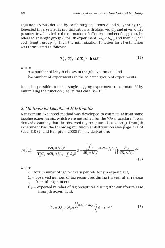
60 Siddeek et al. — Estimating Natural Mortality
Equation 15 was derived by combining equations 8 and 9, ignoring Oljit.Repeated inverse matrix multiplication with observed Cljit and given otherparametric values led to the estimation of effective number of tagged crabsreleased at length group lji for jth experiment, SRlji ¥ Nlji 0, and then SRlji foreach length group lji. Then the minimization function for M estimationwas formulated as follows:
jk
lin SR SR
ji
j= =Â -Â1
21[ln( ) ln( )] (16)
wherenj = number of length classes in the jth experiment, and
k = number of experiments in the selected group of experiments.
It is also possible to use a single tagging experiment to estimate M byminimizing the function (16). In that case, k = 1.
2. Multinomial Likelihood M EstimatorA maximum likelihood method was developed to estimate M from sometagging experiments, which were not suited for the VPA procedure. It wasderived assuming that the observed tag recapture data set <Cjt> from jthexperiment had the following multinomial distribution (see page 274 ofSeber [1982] and Hampton [2000] for the derivation):
f CSR N
C SR N C
C
SR NC
SR Njtj j
jt j j jtt
T
t
T
jtt
T
j j
SR N C jt
j jt
TCj j jt
t
T
jt( )( )!
( !)( )!( ) ( )
^^
=¥
¥ - Â’-
Â
¥ ¥’
==
=¥ - Â
=
=0
011
1
0 011
01
(17)
whereT = total number of tag recovery periods for jth experiment,
Cjt = observed number of tag recaptures during tth year after release from jth experiment,
C jt
^
= expected number of tag recaptures during tth year after release from jth experiment,
C SR N e
FZ
ejt j j
F M Myt
t
Zk k jt
k
t
t t^ ( )
( )= ¥ -- + -
-=
-Â
01
1
1d
d (18)
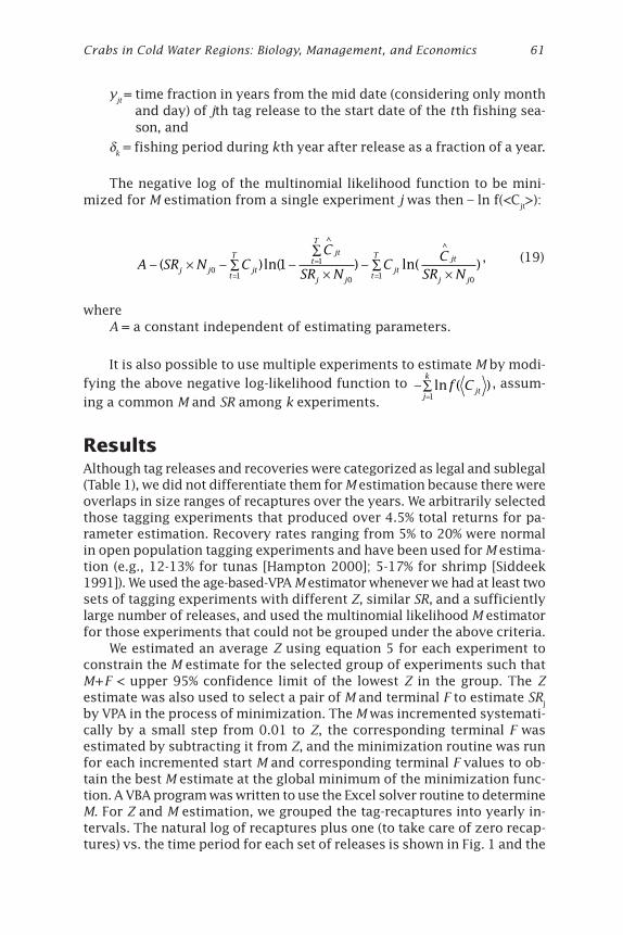
Crabs in Cold Water Regions: Biology, Management, and Economics 61
yjt = time fraction in years from the mid date (considering only monthand day) of jth tag release to the start date of the tth fishing sea-son, and
dk = fishing period during kth year after release as a fraction of a year.
The negative log of the multinomial likelihood function to be mini-mized for M estimation from a single experiment j was then – ln f(<Cjt>):
A SR N C
C
SR NC
CSR Nj j jt
t
T jtt
T
j jjt
t
T jt
j j
- ¥ - Â -Â
¥- Â
¥=
=
=( )ln( ) ln( )
^^
01
1
0 1 0
1 , (19)
whereA = a constant independent of estimating parameters.
It is also possible to use multiple experiments to estimate M by modi-fying the above negative log-likelihood function to
- Â
=ln ( )f Cjt
j
k
1
, assum-ing a common M and SR among k experiments.
ResultsAlthough tag releases and recoveries were categorized as legal and sublegal(Table 1), we did not differentiate them for M estimation because there wereoverlaps in size ranges of recaptures over the years. We arbitrarily selectedthose tagging experiments that produced over 4.5% total returns for pa-rameter estimation. Recovery rates ranging from 5% to 20% were normalin open population tagging experiments and have been used for M estima-tion (e.g., 12-13% for tunas [Hampton 2000]; 5-17% for shrimp [Siddeek1991]). We used the age-based-VPA M estimator whenever we had at least twosets of tagging experiments with different Z, similar SR, and a sufficientlylarge number of releases, and used the multinomial likelihood M estimatorfor those experiments that could not be grouped under the above criteria.
We estimated an average Z using equation 5 for each experiment toconstrain the M estimate for the selected group of experiments such thatM+F < upper 95% confidence limit of the lowest Z in the group. The Zestimate was also used to select a pair of M and terminal F to estimate SRj
by VPA in the process of minimization. The M was incremented systemati-cally by a small step from 0.01 to Z, the corresponding terminal F wasestimated by subtracting it from Z, and the minimization routine was runfor each incremented start M and corresponding terminal F values to ob-tain the best M estimate at the global minimum of the minimization func-tion. A VBA program was written to use the Excel solver routine to determineM. For Z and M estimation, we grouped the tag-recaptures into yearly in-tervals. The natural log of recaptures plus one (to take care of zero recap-tures) vs. the time period for each set of releases is shown in Fig. 1 and the
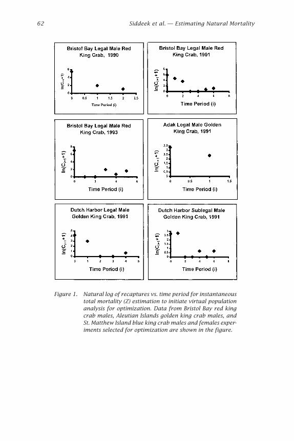
62 Siddeek et al. — Estimating Natural Mortality
Figure 1. Natural log of recaptures vs. time period for instantaneoustotal mortality (Z) estimation to initiate virtual populationanalysis for optimization. Data from Bristol Bay red kingcrab males, Aleutian Islands golden king crab males, andSt. Matthew Island blue king crab males and females exper-iments selected for optimization are shown in the figure.
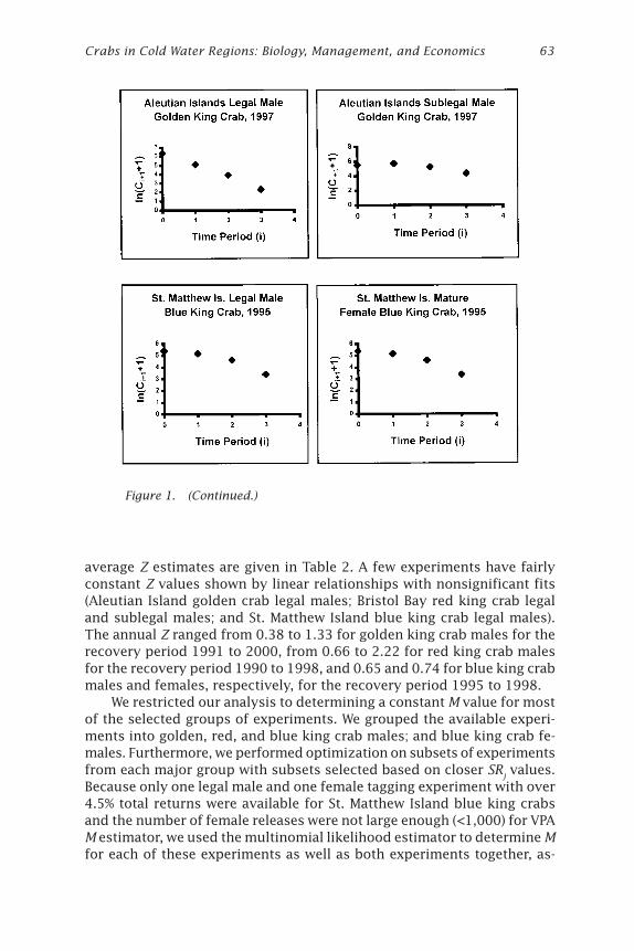
Crabs in Cold Water Regions: Biology, Management, and Economics 63
Figure 1. (Continued.)
average Z estimates are given in Table 2. A few experiments have fairlyconstant Z values shown by linear relationships with nonsignificant fits(Aleutian Island golden crab legal males; Bristol Bay red king crab legaland sublegal males; and St. Matthew Island blue king crab legal males).The annual Z ranged from 0.38 to 1.33 for golden king crab males for therecovery period 1991 to 2000, from 0.66 to 2.22 for red king crab malesfor the recovery period 1990 to 1998, and 0.65 and 0.74 for blue king crabmales and females, respectively, for the recovery period 1995 to 1998.
We restricted our analysis to determining a constant M value for mostof the selected groups of experiments. We grouped the available experi-ments into golden, red, and blue king crab males; and blue king crab fe-males. Furthermore, we performed optimization on subsets of experimentsfrom each major group with subsets selected based on closer SRj values.Because only one legal male and one female tagging experiment with over4.5% total returns were available for St. Matthew Island blue king crabsand the number of female releases were not large enough (<1,000) for VPAM estimator, we used the multinomial likelihood estimator to determine Mfor each of these experiments as well as both experiments together, as-
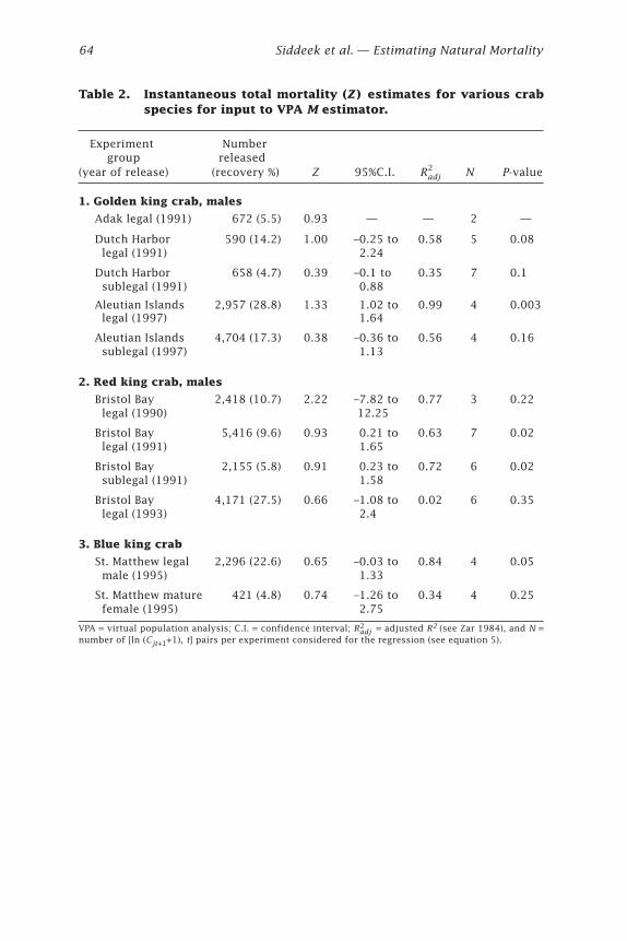
64 Siddeek et al. — Estimating Natural Mortality
Table 2. Instantaneous total mortality (Z ) estimates for various crabspecies for input to VPA M estimator.
Experiment Number group released(year of release) (recovery %) Z 95%C.I. Radj
N P-value
1. Golden king crab, males
Adak legal (1991) 672 (5.5) 0.93 — — 2 —
Dutch Harbor 590 (14.2) 1.00 –0.25 to 0.58 5 0.08 legal (1991) 2.24
Dutch Harbor 658 (4.7) 0.39 –0.1 to 0.35 7 0.1 sublegal (1991) 0.88
Aleutian Islands 2,957 (28.8) 1.33 1.02 to 0.99 4 0.003 legal (1997) 1.64
Aleutian Islands 4,704 (17.3) 0.38 –0.36 to 0.56 4 0.16 sublegal (1997) 1.13
2. Red king crab, males
Bristol Bay 2,418 (10.7) 2.22 –7.82 to 0.77 3 0.22 legal (1990) 12.25
Bristol Bay 5,416 (9.6) 0.93 0.21 to 0.63 7 0.02 legal (1991) 1.65
Bristol Bay 2,155 (5.8) 0.91 0.23 to 0.72 6 0.02 sublegal (1991) 1.58
Bristol Bay 4,171 (27.5) 0.66 –1.08 to 0.02 6 0.35 legal (1993) 2.4
3. Blue king crab
St. Matthew legal 2,296 (22.6) 0.65 –0.03 to 0.84 4 0.05 male (1995) 1.33
St. Matthew mature 421 (4.8) 0.74 –1.26 to 0.34 4 0.25 female (1995) 2.75
VPA = virtual population analysis; C.I. = confidence interval; Radj = adjusted R2 (see Zar 1984), and N =
number of [ln (Cjt+1+1), t] pairs per experiment considered for the regression (see equation 5).
2
2
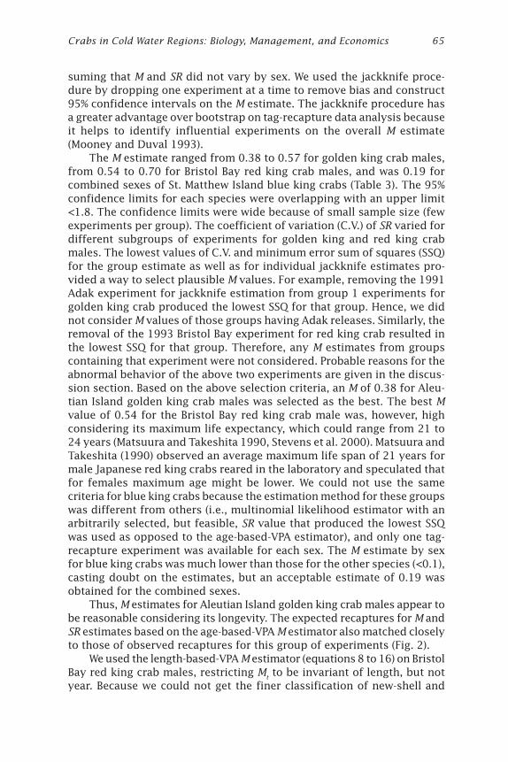
Crabs in Cold Water Regions: Biology, Management, and Economics 65
suming that M and SR did not vary by sex. We used the jackknife proce-dure by dropping one experiment at a time to remove bias and construct95% confidence intervals on the M estimate. The jackknife procedure hasa greater advantage over bootstrap on tag-recapture data analysis becauseit helps to identify influential experiments on the overall M estimate(Mooney and Duval 1993).
The M estimate ranged from 0.38 to 0.57 for golden king crab males,from 0.54 to 0.70 for Bristol Bay red king crab males, and was 0.19 forcombined sexes of St. Matthew Island blue king crabs (Table 3). The 95%confidence limits for each species were overlapping with an upper limit<1.8. The confidence limits were wide because of small sample size (fewexperiments per group). The coefficient of variation (C.V.) of SR varied fordifferent subgroups of experiments for golden king and red king crabmales. The lowest values of C.V. and minimum error sum of squares (SSQ)for the group estimate as well as for individual jackknife estimates pro-vided a way to select plausible M values. For example, removing the 1991Adak experiment for jackknife estimation from group 1 experiments forgolden king crab produced the lowest SSQ for that group. Hence, we didnot consider M values of those groups having Adak releases. Similarly, theremoval of the 1993 Bristol Bay experiment for red king crab resulted inthe lowest SSQ for that group. Therefore, any M estimates from groupscontaining that experiment were not considered. Probable reasons for theabnormal behavior of the above two experiments are given in the discus-sion section. Based on the above selection criteria, an M of 0.38 for Aleu-tian Island golden king crab males was selected as the best. The best Mvalue of 0.54 for the Bristol Bay red king crab male was, however, highconsidering its maximum life expectancy, which could range from 21 to24 years (Matsuura and Takeshita 1990, Stevens et al. 2000). Matsuura andTakeshita (1990) observed an average maximum life span of 21 years formale Japanese red king crabs reared in the laboratory and speculated thatfor females maximum age might be lower. We could not use the samecriteria for blue king crabs because the estimation method for these groupswas different from others (i.e., multinomial likelihood estimator with anarbitrarily selected, but feasible, SR value that produced the lowest SSQwas used as opposed to the age-based-VPA estimator), and only one tag-recapture experiment was available for each sex. The M estimate by sexfor blue king crabs was much lower than those for the other species (<0.1),casting doubt on the estimates, but an acceptable estimate of 0.19 wasobtained for the combined sexes.
Thus, M estimates for Aleutian Island golden king crab males appear tobe reasonable considering its longevity. The expected recaptures for M andSR estimates based on the age-based-VPA M estimator also matched closelyto those of observed recaptures for this group of experiments (Fig. 2).
We used the length-based-VPA M estimator (equations 8 to 16) on BristolBay red king crab males, restricting Mt to be invariant of length, but notyear. Because we could not get the finer classification of new-shell and
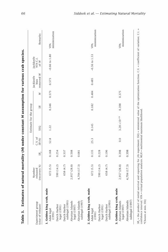
66 Siddeek et al. — Estimating Natural Mortality
Tab
le 3
.Esti
mate
s o
f n
atu
ral
mort
ali
ty (
M)
un
der
con
sta
nt
M a
ssu
mp
tion
for
vari
ou
s c
rab
sp
ecie
s.
SRj
= t
he
pro
du
ct o
f in
itia
l su
r viv
al a
nd
rep
or t
ing f
or
j th
exp
erim
ent;
SSQ
= m
inim
ized
val
ue
of
the
op
tim
izat
ion
fu
nct
ion
; C
.V.
= c
oef
fici
ent
of
var
iati
on
; C
.I.
=co
nfi
den
ce i
nte
r val
; V
PA =
vir
tual
po
pu
lati
on
an
alysi
s; M
LH =
mu
ltin
om
ial
max
imu
m l
ikel
iho
od
.a C
ho
sen
at
min
. SS
Q
1.
Gold
en
kin
g c
rab
, m
ale
Ad
ak l
egal
67
2 (
5.5
)0
.16
85
2.8
1.2
20
.34
60
.57
30
.57
3–0
.66
to 1
.80
VPA
(1
99
1)
min
imiz
atio
n
Du
tch
Har
bor
59
0 (
14
.2)
0.2
54
le
gal
(1
99
1)
Du
tch
Har
bor
65
8 (
4.7
)0
.33
7
sub
legal
(1
99
1)
Ale
uti
an I
slan
ds
2,9
57
(2
8.8
)0
.50
8
legal
(1
99
7)
Ale
uti
an I
slan
ds
4,7
04
(1
7.3
)0
.68
1
sub
legal
(1
99
7)
2.
Gold
en
kin
g c
rab
, m
ale
Ad
ak l
egal
67
2 (
5.5
)0
.13
52
5.3
0.1
45
0.1
82
0.4
84
0.4
85
–0.5
6 t
o 1
.53
VPA
(1
99
1)
m
inim
izat
ion
Du
tch
Har
bor
59
0 (
14
.2)
0.2
28
le
gal
(1
99
1)
Du
tch
Har
bor
65
8 (
4.7
)0
.19
6
sub
legal
(1
99
1)
3.
Gold
en
kin
g c
rab
, m
ale
Ale
uti
an I
slan
ds
2,9
57
(2
8.8
)0
.39
80
.03
.28
¥ 1
0–1
90
.39
80
.37
5V
PA
legal
(1
99
7)
m
inim
izat
ion
Ale
uti
an Isl
and
s4,7
04 (17.3
)0.3
98
su
ble
gal (1
997)
Est
imat
e fo
r th
e gro
up
Nu
mb
er
Jack
kn
ife
Jack
kn
ife
Exp
erim
ent
gro
up
r
elea
sed
C.V
. o
f
b
ias
95
% C
.I.
(yea
r o
f re
leas
e)
(
reco
ver
y %
)
SRj
SR
(%
)
SS
Q
S
R
M
re
mo
ved
M
o
f M
R
emar
ks
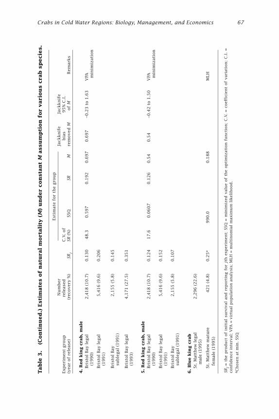
Crabs in Cold Water Regions: Biology, Management, and Economics 67
Tab
le 3
.(C
on
tin
ued
.) E
sti
mate
s o
f n
atu
ral
mort
ali
ty (
M)
un
der
con
sta
nt
M a
ssu
mp
tion
for
vari
ou
s c
rab
sp
ecie
s.
SRj
= t
he
pro
du
ct o
f in
itia
l su
r viv
al a
nd
rep
or t
ing f
or
j th
exp
erim
ent;
SSQ
= m
inim
ized
val
ue
of
the
op
tim
izat
ion
fu
nct
ion
; C
.V.
= c
oef
fici
ent
of
var
iati
on
; C
.I.
=co
nfi
den
ce i
nte
r val
; V
PA =
vir
tual
po
pu
lati
on
an
alysi
s; M
LH =
mu
ltin
om
ial
max
imu
m l
ikel
iho
od
.a C
ho
sen
at
min
. SS
Q
4.
Red
kin
g c
rab
, m
ale
Bri
stol
Bay
leg
al2
,41
8 (
10
.7)
0.1
30
48
.30
.59
70
.19
20
.69
70
.69
7–0
.23
to 1
.63
VPA
(1
99
0)
m
inim
izat
ion
Bri
stol
Bay
leg
al5
,41
6 (
9.6
)0
.20
6
(19
91
)
Bri
stol
Bay
2,1
55
(5
.8)
0.1
45
su
ble
gal
(1
99
1)
Bri
stol
Bay
leg
al4
,17
1 (
27
.5)
0.3
51
(1
99
3)
5.
Red
kin
g c
rab
, m
ale
Bri
stol
Bay
leg
al2
,41
8 (
10
.7)
0.1
24
17
.60
.06
07
0.1
26
0.5
40
.54
–0.4
2 t
o 1
.50
VPA
(1
99
0)
m
inim
izat
ion
Bri
stol
Bay
leg
al5
,41
6 (
9.6
)0
.15
2
(19
91
)
Bri
stol
Bay
2,1
55
(5
.8)
0.1
07
su
ble
gal
(1
99
1)
6.
Blu
e k
ing c
rab
St.
Mat
thew
leg
al2
,29
6 (
22
.6)
m
ale
(19
95
)
St.
Mat
thew
mat
ure
42
1 (
4.8
)0
.25
a
99
0.0
0.1
88
MLH
fe
mal
e (1
99
5)
Es
tim
ate
for
the
gro
up
Nu
mb
er
Jack
kn
ife
Jack
kn
ife
Exp
erim
ent
gro
up
r
elea
sed
C.V
. o
f
b
ias
95
% C
.I.
(yea
r o
f re
leas
e)
(
reco
ver
y %
)
SRj
SR
(%
)
SS
Q
S
R
M
re
mo
ved
M
o
f M
R
emar
ks
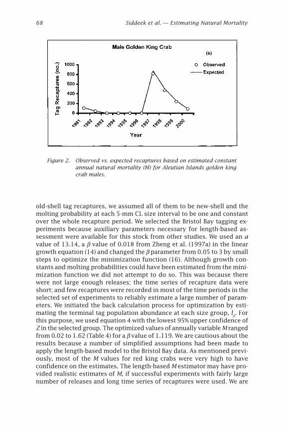
68 Siddeek et al. — Estimating Natural Mortality
old-shell tag recaptures, we assumed all of them to be new-shell and themolting probability at each 5-mm CL size interval to be one and constantover the whole recapture period. We selected the Bristol Bay tagging ex-periments because auxiliary parameters necessary for length-based as-sessment were available for this stock from other studies. We used an avalue of 13.14, a b value of 0.018 from Zheng et al. (1997a) in the lineargrowth equation (14) and changed the b parameter from 0.05 to 3 by smallsteps to optimize the minimization function (16). Although growth con-stants and molting probabilities could have been estimated from the mini-mization function we did not attempt to do so. This was because therewere not large enough releases; the time series of recapture data wereshort; and few recaptures were recorded in most of the time periods in theselected set of experiments to reliably estimate a large number of param-eters. We initiated the back calculation process for optimization by esti-mating the terminal tag population abundance at each size group, lji. Forthis purpose, we used equation 4 with the lowest 95% upper confidence ofZ in the selected group. The optimized values of annually variable M rangedfrom 0.02 to 1.62 (Table 4) for a b value of 1.119. We are cautious about theresults because a number of simplified assumptions had been made toapply the length-based model to the Bristol Bay data. As mentioned previ-ously, most of the M values for red king crabs were very high to haveconfidence on the estimates. The length-based M estimator may have pro-vided realistic estimates of M, if successful experiments with fairly largenumber of releases and long time series of recaptures were used. We are
Figure 2. Observed vs. expected recaptures based on estimated constantannual natural mortality (M) for Aleutian Islands golden kingcrab males.
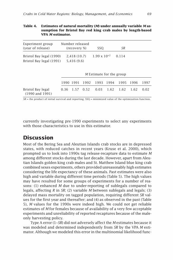
Crabs in Cold Water Regions: Biology, Management, and Economics 69
Table 4. Estimates of natural mortality (M) under annually variable M as-sumption for Bristol Bay red king crab males by length-basedVPA M estimator.
Experiment group Number released(year of release) (recovery %) SSQ SR
Bristol Bay legal (1990) 2,418 (10.7) 1.99 x 10+2 0.114
Bristol Bay legal (1991) 5,416 (9.6)
M Estimate for the group
1990 1991 1992 1993 1994 1995 1996 1997
Bristol Bay legal 0.36 1.57 0.52 0.03 1.62 1.62 1.62 0.02 (1990 and 1991)
SR = the product of initial survival and reporting; SSQ = minimized value of the optimization function.
currently investigating pre-1990 experiments to select any experimentswith those characteristics to use in this estimator.
DiscussionMost of the Bering Sea and Aleutian Islands crab stocks are in depressedstates, with reduced catches in recent years (Kruse et al. 2000), whichprompted us to look into 1990s tag release-recapture data to estimate Mamong different stocks during the last decade. However, apart from Aleu-tian Islands golden king crab males and St. Matthew Island blue king crabcombined sexes experiments, others provided unreasonably high estimatesconsidering the life expectancy of these animals. Past estimates were alsohigh and variable during different time periods (Table 5). The high valuesmay have resulted for some groups of experiments for a number of rea-sons: (1) enhanced M due to under-reporting of sublegals compared tolegals, affecting R in SR; (2) variable M between sublegals and legals; (3)delayed mass mortality on tagged population, requiring different SR val-ues for the first year and thereafter; and (4) as observed in the past (Table5), M values for the 1990s were indeed high. We could not get reliableestimates of M for females because of availability of a very few acceptableexperiments and unreliability of reported recaptures because of the male-only harvesting policy.
Type A error (1–SR) did not adversely affect the M estimates because itwas modeled and determined independently from SR by the VPA M esti-mator. Although we modeled this error in the multinomial likelihood func-
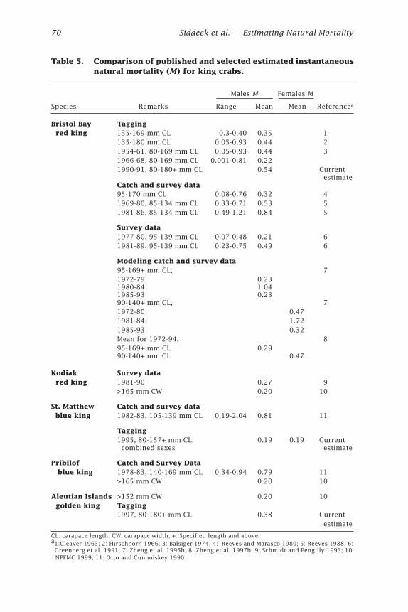
70 Siddeek et al. — Estimating Natural Mortality
Table 5. Comparison of published and selected estimated instantaneousnatural mortality (M) for king crabs.
Males M Females M
Species Remarks Range Mean Mean Referencea
Bristol Bay Tagging red king 135-169 mm CL 0.3-0.40 0.35 1
135-180 mm CL 0.05-0.93 0.44 21954-61, 80-169 mm CL 0.05-0.93 0.44 31966-68, 80-169 mm CL 0.001-0.81 0.221990-91, 80-180+ mm CL 0.54 Current
estimateCatch and survey data95-170 mm CL 0.08-0.76 0.32 41969-80, 85-134 mm CL 0.33-0.71 0.53 51981-86, 85-134 mm CL 0.49-1.21 0.84 5
Survey data1977-80, 95-139 mm CL 0.07-0.48 0.21 61981-89, 95-139 mm CL 0.23-0.75 0.49 6
Modeling catch and survey data95-169+ mm CL, 71972-79 0.231980-84 1.041985-93 0.2390-140+ mm CL, 71972-80 0.471981-84 1.721985-93 0.32Mean for 1972-94, 895-169+ mm CL 0.2990-140+ mm CL 0.47
Kodiak Survey data red king 1981-90 0.27 9
>165 mm CW 0.20 10
St. Matthew Catch and survey data blue king 1982-83, 105-139 mm CL 0.19-2.04 0.81 11
Tagging1995, 80-157+ mm CL, 0.19 0.19 Current combined sexes estimate
Pribilof Catch and Survey Data blue king 1978-83, 140-169 mm CL 0.34-0.94 0.79 11
>165 mm CW 0.20 10
Aleutian Islands >152 mm CW 0.20 10 golden king Tagging
1997, 80-180+ mm CL 0.38 Current estimate
CL: carapace length; CW: carapace width; +: Specified length and above.a1:Cleaver 1963; 2: Hirschhorn 1966; 3: Balsiger 1974; 4: Reeves and Marasco 1980; 5: Reeves 1988; 6: Greenberg et al. 1991; 7: Zheng et al. 1995b; 8: Zheng et al. 1997b; 9: Schmidt and Pengilly 1993; 10:
NPFMC 1999; 11: Otto and Cummiskey 1990.
Crabs in Cold Water Regions: Biology, Management, and Economics 71
tion, we did not estimate it through the model because of availability of afew acceptable tagging experiments for blue king crabs. However, we choseacceptable SR values based on lowest SSQ after trial runs of optimizationon blue king crab data. Type A error was high in all experiments and rangedfrom 0.52 to 0.89 for golden and red king crab males. This emphasizedthe need for a large number of releases for plausible mortality estimation.The M estimates may be inflated due to continuous tag shedding, system-atic tagging mortality, and emigration (Ricker’s type B error). Pengilly andWatson (1992) observed that Floy tag loss from red king crabs in holdingtanks was virtually nonexistent. The loss rate of tags from deepwater goldenking crab was not known. Because the loss rate in their natural environ-ment was largely unknown and difficult to model independently from M,we assumed Type B error to be negligible. Nearly 97% of recaptures fromthe 1991 Adak experiment were reported during the first two years afterrelease and 99% of recaptures from the 1993 Bristol Bay experiment werereported during the first year after release (Table 1), suggesting an en-hanced catchability on tagged population during the initial years of theseexperiments. This may have been due to abnormal behavior or nonran-dom mixing of tagged crabs, or nonrandom distribution of effort duringthe first two seasons after the release and is known as Ricker’s type Cerror. The jackknife procedure was useful to detect this type of abnormalexperiments, and thus we were able to choose M from the group that ex-cluded abnormal experiments.
Minimum variation among ln(SRj) for a selected group of experimentswas a critical assumption for successful optimization. The M estimateswere selected from those groups having smaller CV of SR (Table 3). Thus,the constant ln(SR) assumption within the selected group was satisfied.The best estimates of M for golden and red king crab males were selectedfrom groups with individual releases exceeding 2000; thus, the numerousreleases assumption for deterministic mortality processes was also satis-fied.
The size-specific natural mortality (Mlji) can be introduced in the newlength-based-VPA M estimator and the multinomial likelihood M estimator(Hampton 2000) for parameter estimation. In the past, size-specific M es-timates have been reported from tag-recapture analysis (Hirschhorn 1966,Balsiger 1974). However, we opted not to pursue along this line with thecurrent data for the following reasons. First, because recaptures were mixedwith new- and old-shell crabs, M within a size class may not be a constant.Due to different molting probabilities, in a given size range one could findan old crab that had not molted in a given year as well as a younger crabthat had molted into that size class from a smaller size group in that year.Second, the tag recovery periods extended to a few years, 2 to 7 at mostwith few number of recaptures (Table 1); thus, number of data points werenot sufficient to estimate a large number of parameters with precision.Third, the primary objective of this paper was to obtain an average con-stant M, if possible, for direct application to currently used crab stock
72 Siddeek et al. — Estimating Natural Mortality
assessment and management procedures. A major drawback of size-spe-cific M estimator is the assumption of length-invariant SR, which may nothold for experiments with a wider size range of releases. However, onemay select a subset of appropriate length classes to keep SRj fairly con-stant among them to obtain successful optimization.
The age-based-VPA M estimator has a greater advantage over its length-based counterpart on crab mortality estimation from tag-recapture databecause a crab’s complex growth process (growth is a function of moltincrement and molting probability) could be ignored in the former, thusreducing the number of estimating parameters in the model. However, itrequires successful experiments with numerous releases, similar SR val-ues, and different total mortality values for plausible M estimation. On theother hand, the new length-based-VPA M estimator could be used with asingle successful experiment with numerous releases and recaptures forsuccessful optimization provided conditions specified in the previousparagraph are met.
AcknowledgmentsFunding for the Aleutian Islands, Bristol Bay, and St. Matthew Island crabsurveys was provided through the State of Alaska Bering Sea test fish pro-gram. We appreciate the technical and logistic help provided by DouglasPengilly of the Department of Fish and Game, Division of CommercialFisheries, Kodiak. We thank Gordon Kruse and Jie Zheng of ADFG andanonymous reviewers for their suggestions to improve this presentation.This study is funded in part by cooperative agreement NA97FN0129 fromthe National Oceanic and Atmospheric Administration (NOAA). The viewsexpressed herein are those of the authors and do not necessarily reflectthe views of NOAA or any of its subagencies. This is contribution PP 212 ofthe Alaska Department of Fish and Game, Division of Commercial Fisher-ies, Juneau.
ReferencesBalsiger, J.W. 1974. A computer simulation model for the south eastern Bering Sea
king crab population. Ph.D. thesis, University of Washington, Seattle. 198 pp.
Blau, S.F. 1996. The 1995 St. Matthew Island blue king crab survey. Alaska Depart-ment of Fish and Game, Division of Commercial Fisheries, Regional Informa-tion Report 4K96-27, Kodiak.
Blau, S.F., and D. Pengilly. 1994. Findings from the 1991 golden king crab survey inthe Dutch Harbor and Adak management areas including analysis of recov-ered tagged crabs. Alaska Department of Fish and Game, Division of Commer-cial Fisheries, Regional Information Report 4K94-35, Kodiak.
Crabs in Cold Water Regions: Biology, Management, and Economics 73
Blau, S.F., and L.J. Watson. 1999. St. Matthew Island blue king crab survey, 1998.Alaska Department of Fish and Game, Division of Commercial Fisheries, Re-gional Information Report 4K99-66, Kodiak.
Blau, S.F., L.J. Watson, and I. Vining. 1998. The 1997 Aleutian Islands golden kingcrab survey. Alaska Department of Fish and Game, Division of CommercialFisheries, Regional Information Report 4K98-30, Kodiak.
Cleaver, F.C. 1963. Bering Sea king crab (Paralithodes camtschaticus) tagging exper-iments. In: ICNAF North Atlantic Fish Marketing Symposium. Int. Comm. North-west Atl. Fish. Spec. Publ. 4:59-63.
Gray, G.W. Jr. 1965. Tags for marking king crabs. Prog. Fish-Cult. 27:221-227.
Greenberg, J.A., S.C. Matulich, and R.C. Mittelhammer. 1991. A system of equationsapproach to modeling age structured fish populations: The case of Alaskanred king crab, Paralithodes camtschaticus. Can. J. Fish. Aquat. Sci. 48:1613-1622.
Hampton, J. 2000. Natural mortality rates in tropical tunas: Size really does matter.Can. J. Fish. Aquat. Sci. 57:1002-1010.
Hirschhorn, G. 1966. Variation in biomass of eastern Bering Sea king crabs basedon tagging estimates of growth and mortality. Int. North Pac. Fish. Comm. Doc.909.
Kruse, G.H., F.C. Funk, H.J. Geiger, K.R. Mabry, H.M. Savikko, and S.M. Siddeek.2000. Overview of state-managed marine fisheries in the central and westernGulf of Alaska, Aleutian Islands, and southeastern Bering Sea, with referenceto Steller sea lions. Alaska Department of Fish and Game, Division of Commer-cial Fisheries, Regional Information Report No. 5J00-10, Juneau. 173 pp.
Matsuura, S., and K. Takeshita. 1990. Longevity of red king crab, Paralithodescamtschatica, revealed by long-term rearing study. In: Proceedings of the In-ternational Symposium on King and Tanner Crabs. University of Alaska SeaGrant, AK-SG-90-04, Fairbanks, pp. 181-188.
Mooney, C.Z., and R.D. Duval. 1993. Bootstrapping: A nonparametric approach tostatistical inference. Sage university paper series: Quantitative applications inthe social sciences, 95. Sage Publications, Inc. 73 pp.
NPFMC (North Pacific Fishery Management Council). 1999. Draft for secretarial re-view: Environmental assessment for Amendment 7 to the fishery managementplan for the commercial king and Tanner crab fisheries in the Bering Sea/Aleutian Islands to 1. Revise definitions of overfishing, MSY, and OY; 2. Updatethe BSAI crab FMP. Prepared by NPFMC, ADFG, NMFS, and UA staff. 50 pp.
Otto, R.S., and P.A. Cummiskey. 1990. Growth of adult male blue crab (Paralithodesplatypus). In: Proceedings of the International Symposium on King and TannerCrabs. University of Alaska Sea Grant, AK-SG-90-04, Fairbanks, pp. 245-257.
Pengilly, D., and L.J. Watson. 1992. Visible (floy) and non-visible (pit) tag retentionexperiments and automated pit tag detection trials conducted on Bristol Bayred king crab in 1991. Alaska Department of Fish and Game, Division of Com-mercial Fisheries, Regional Information Report 4K92-28, Kodiak.

74 Siddeek et al. — Estimating Natural Mortality
Pope, J.G. 1972. An investigation of the accuracy of virtual population analysisusing cohort analysis. Int. Comm. Northwest Atl. Fish. Res. Bull. 9:65-74.
Reeves, J.E. 1988. A biological assessment of the minimum size limit for BristolBay red king crab. NOAA Tech. Memo. NMFS F/NWC-133, Seattle, Washington.64 pp.
Reeves, J.E., and R. Marasco. 1980. An evaluation of alternate management optionsfor the southern Bering Sea king crab fishery. NWAFC Processed Report 80-6.National Marine Fisheries Service, Northwest Alaska Fisheries Center, Seattle,Washington. 85 pp.
Restrepo, V.R., G.G. Thompson, P.M. Mace, W.L. Gabriel, L.L. Low, A.D. MacCall, R.D.Methot, J.E. Powers, B.L. Taylor, P.R. Wade, and J.F. Witzig. 1998. Technicalguidance on the use of precautionary approaches to implementing nationalstandard 1 of the Magnuson-Stevens Fishery Conservation and ManagementAct. NOAA Tech. Memo. NMFS-F/SPO-31. 54 pp.
Ricker, W.E. 1975. Computation and interpretation of biological statistics of fishpopulations. Department of the Environment Fisheries and Marine Service,Bulletin 191, Ottawa. 382 pp.
Schmidt, D.C., and D. Pengilly. 1993. Review of harvest strategies used in the manage-ment of lithodid crab in Alaska. In: G. Kruse, D.M. Eggers, R.J. Marasco, C. Pautzke,and T.J. Quinn II (eds.), Proceedings of the International Symposium on Man-agement Strategies for Exploited Fish Populations. University of Alaska SeaGrant, AK-SG-93-02, Fairbanks, pp. 385-407.
Seber, G.A.F. 1982. The estimation of animal abundance and related parameters,2nd edn. Macmillan, New York. 645 pp.
Siddeek, M.S.M. 1989. The estimation of natural mortality in Irish Sea plaice Pleuro-nectes platessa L. using tagging methods. J. Fish. Biol. 35(Suppl. A):145-154.
Siddeek, M.S.M. 1991. Estimation of natural mortality of Kuwait’s grooved tigerprawn Penaeus semisulcatus (de Haan) using tag-recapture and commercialfisheries data. Fish. Res. 11:109-125.
Silliman, R.P. 1943. Studies on the Pacific pilchard or sardine (Sardinops caerulea),5: A method of computing mortalities and replacements. U.S. Fish Wildl. Serv.Spec. Sci. Rep. Fish. 24:235-242.
Stevens, B.G., J.A. Haaga, R.A. MacIntosh, R.S. Otto, and L. Rugolo. 2000. AFSC pro-cessed report 2000-07: Report to the industry on the 2000 eastern Bering Seacrab survey, November 2000. National Marine Fisheries Service, Alaska Fisher-ies Science Center, Kodiak Fisheries Research Center, Kodiak.
Sullivan, P.J., H.L. Lai, and V.F. Gallucci. 1990. A catch-at-length analysis that incor-porates a stochastic model of growth. Can. J. Fish. Aquat. Sci. 47:184-198.
Wallace, M.M., C.J. Pertuit, and A.R. Hvatum. 1949. Contribution to the biology ofthe king crab (Paralithodes camtschatica Tilesius). U.S. Fish and Wildlife Ser-vice Leaflet 340. 50 pp.
Crabs in Cold Water Regions: Biology, Management, and Economics 75
Watson, L.J., and D. Pengilly. 1994. Project operational plan for the 1993 Bristol Bayred king crab test fishery project. Alaska Department of Fish and Game, Divi-sion of Commercial Fisheries, Regional Information Report 4K94-27, Kodiak.
Zar, J.H. 1984. Biostatistical analysis, 2nd edn. Prentice Hall, New Jersey. 718 pp.
Zheng, J., M.C. Murphy, and G.H. Kruse. 1995a. A length-based population modeland stock-recruitment relationships for red king crab, Paralithodes camtschat-icus, in Bristol Bay, Alaska. Can. J. Fish. Aquat. Sci. 52:1229-1246.
Zheng, J., M.C. Murphy, and G.H. Kruse. 1995b. Updated length-based populationmodel and stock-recruitment relationships for red king crab in Bristol Bay,Alaska. Alaska Fish. Res. Bull. 2(2):114-124.
Zheng, J., M.C. Murphy, and G.H. Kruse. 1997a. Analysis of harvest strategies forred king crab, Paralithodes camtschaticus, in Bristol Bay, Alaska. Can. J. Fish.Aquat. Sci. 54:1121-1134.
Zheng, J., M.C. Murphy, and G.H. Kruse. 1997b. Alternative rebuilding strategiesfor the red king crab Paralithodes camtschaticus fishery in Bristol Bay, Alaska.J. Shellfish Res. 16(1):205-217.

Crabs in Cold Water Regions: Biology, Management, and Economics 77Alaska Sea Grant College Program • AK-SG-02-01, 2002
Estimating Molting Probabilitiesof Female Dungeness Crabs(Cancer magister) in NorthernCalifornia: A Multi-Stage LatentVariable ApproachQian-Li XueThe Johns Hopkins University, Department of Epidemiology,Baltimore, Maryland
David G. HankinDepartment of Fisheries, Humboldt State University, Arcata, California
Extended AbstractEstimation of size-specific molting probabilities of crustaceans has oftenbeen based on indirect indicators of molting status including visual orchemical methods applied to internal or external features that reflect re-cent molting or molting failure. Mohr and Hankin (1989) proposed a maxi-mum likelihood estimator of size-specific molting probabilities, based onshell condition, a postmolt indicator. The validity of the Mohr-Hankin es-timator hinges upon two key assumptions: (1) a well-defined molting sea-son of relatively short duration, and (2) high classification accuracy.Satisfying condition 1 poses little problem for some crustaceans, includ-ing the Dungeness crab. The validity of assumption 2, however, could bequestionable. All postmolt indicators arguably measure molting statuswith error due to various causes, including at least variation among ob-servers, time elapsed since crabs last molted, and imperfect repeatabilityof classifications. It is well known that the misclassification will lead tobiased inferences (Chen 1989). This study aims to develop improved esti-mators of size-specific molting probabilities that account for the imper-fections in classification of molting status.
We propose a regression model that treats postmolt indicators as sur-rogates for true molt status. We argue that this method addresses bothanalytic challenges identified above. Specifically, we propose a two-stage
78 Xue and Hankin — Estimating Molting Probabilities
procedure that first synthesizes observed information to probabilisticallydetermine true molting status, and then analyzes the association betweenthe true molting status and other covariates via logistic regression; forexample, how premolt carapace width relates to molting probability dur-ing the upcoming season. Our approach to estimating model parametersis similar to pseudo maximum likelihood (Gong and Samaniego 1981).
We illustrate application of our estimator using postmolt shell condi-tion and sperm plug data collected from the northern California popula-tion of adult female Dungeness crabs (Cancer magister). Adult femaleDungeness crabs are known to exhibit a well-defined annual molting sea-son extending from mid-February through mid-May in northern Califor-nia. On the basis of visual inspection of carapace condition (degree ofdeterioration, fouling, and discoloration), the molting history of femalecrabs with respect to the previous molting season was classified into oneof five classes: (1) definitely molted, (2) probably molted, (2.5) impossibleto judge, (3) probably did not molt, and (4) definitely did not molt. Be-cause molting is an essential prerequisite for females to successfully matewith males, a definitive indicator of recent mating activity, if one exists,would allow more reliable assessments of molting success than could beobtained from the shell condition data alone. A recent study (Oh 2000)has provided empirical evidence that presence (or absence) of sperm plugswithin the females’ vaginal tracts in Dungeness crabs is a definitive indica-tor of mating/molting success (or failure) for crabs with postseason cara-pace width (CW) greater than 120 mm (D.G. Hankin, unpubl. observations).Although presence of sperm plugs has been found to be the most reliableindicator of molting status, its use is limited by the need to sacrifice ani-mals. In contrast, shell condition data can be inexpensively and quicklyobtained and hence are more practical for the purpose of estimating molt-ing probabilities in a large sample setting. Comparison of shell conditionassessments with sperm plug data revealed that (a) essentially all class 1crabs (≥120 mm CW) had sperm plugs; (b) essentially no class 2.5 or highercrabs had sperm plugs; and (c) class 2 crabs proved to contain a mixtureof molted and nonmolted crabs (D.G. Hankin, unpubl. observations). Ouranalysis effectively corrects such imperfections in shell classification.
To estimate molting probabilities, we developed a four-stage fittingalgorithm. In stage 1 we calculated the probability p1 (p0) that a crab iscorrectly classified as having (not having) molted, based on sperm plugdata from a substudy. In stage 2 we estimated molting probabilities givenshell condition data from field samples using Bayes’ theorem, while fixingp0 and p1 at their estimates from the first stage. We also assumed that theratio, R, of size-independent survival probabilities through the moltingseason for molting as compared with nonmolting crabs is known. In stage3 we randomly assigned molting status to each crab using its estimatedconditional probability of molting given its shell classification and recon-structed the premolt size distribution according to molting status using awell-defined premolt-postmolt size relationship (Mohr and Hankin 1989).
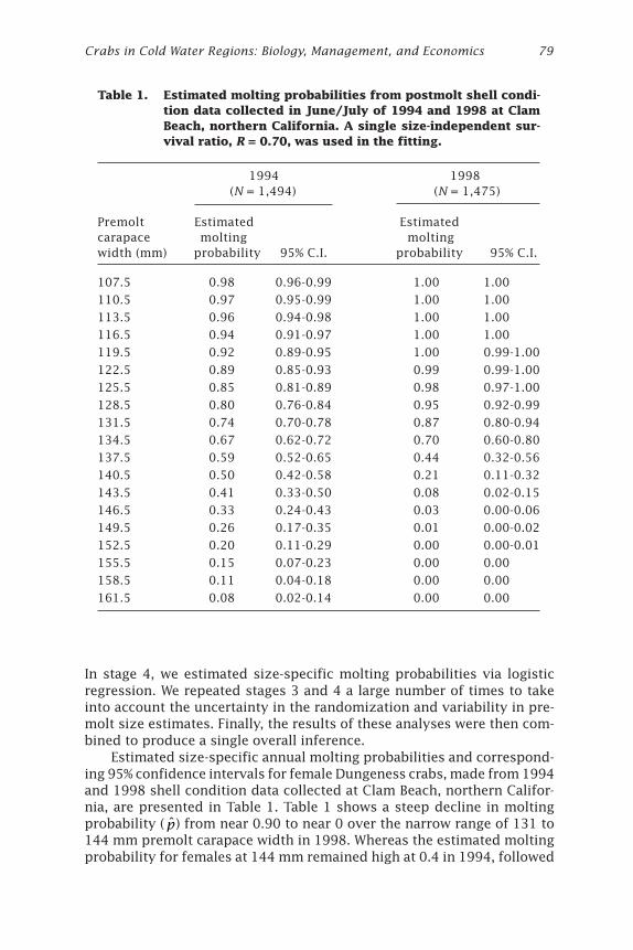
Crabs in Cold Water Regions: Biology, Management, and Economics 79
In stage 4, we estimated size-specific molting probabilities via logisticregression. We repeated stages 3 and 4 a large number of times to takeinto account the uncertainty in the randomization and variability in pre-molt size estimates. Finally, the results of these analyses were then com-bined to produce a single overall inference.
Estimated size-specific annual molting probabilities and correspond-ing 95% confidence intervals for female Dungeness crabs, made from 1994and 1998 shell condition data collected at Clam Beach, northern Califor-nia, are presented in Table 1. Table 1 shows a steep decline in moltingprobability ( ̂p) from near 0.90 to near 0 over the narrow range of 131 to144 mm premolt carapace width in 1998. Whereas the estimated moltingprobability for females at 144 mm remained high at 0.4 in 1994, followed
Table 1. Estimated molting probabilities from postmolt shell condi-tion data collected in June/July of 1994 and 1998 at ClamBeach, northern California. A single size-independent sur-vival ratio, R = 0.70, was used in the fitting.
1994 1998 (N = 1,494) (N = 1,475)
Premolt Estimated Estimatedcarapace molting moltingwidth (mm) probability 95% C.I. probability 95% C.I.
107.5 0.98 0.96-0.99 1.00 1.00
110.5 0.97 0.95-0.99 1.00 1.00
113.5 0.96 0.94-0.98 1.00 1.00
116.5 0.94 0.91-0.97 1.00 1.00
119.5 0.92 0.89-0.95 1.00 0.99-1.00
122.5 0.89 0.85-0.93 0.99 0.99-1.00
125.5 0.85 0.81-0.89 0.98 0.97-1.00
128.5 0.80 0.76-0.84 0.95 0.92-0.99
131.5 0.74 0.70-0.78 0.87 0.80-0.94
134.5 0.67 0.62-0.72 0.70 0.60-0.80
137.5 0.59 0.52-0.65 0.44 0.32-0.56
140.5 0.50 0.42-0.58 0.21 0.11-0.32
143.5 0.41 0.33-0.50 0.08 0.02-0.15
146.5 0.33 0.24-0.43 0.03 0.00-0.06
149.5 0.26 0.17-0.35 0.01 0.00-0.02
152.5 0.20 0.11-0.29 0.00 0.00-0.01
155.5 0.15 0.07-0.23 0.00 0.00
158.5 0.11 0.04-0.18 0.00 0.00
161.5 0.08 0.02-0.14 0.00 0.00
80 Xue and Hankin — Estimating Molting Probabilities
by a gradual decline to less than 0.1 at carapace widths exceeding 158 mmCW. In view of these findings, we conclude that interannual variation insize-specific molting probabilities may make a substantial contribution tobetween-year variation in growth and reproductive potential of femaleDungeness crabs.
In summary, in this paper we developed a new approach to estimatingsize-specific molting probabilities for species that exhibit a well-definedmolting season. By incorporating sperm plug data from the substudy formolting status calibration, the proposed method effectively diminishesthe bias resulting from potential misclassification of shell condition inmolting probability estimation.
ReferencesChen, T.T. 1989. A review of methods for misclassified categorical data in epidemi-
ology. Stat. Med. 8:95-106.
Gong, G., and F.J. Samaniego. 1981. Pseudo maximum likelihood estimation: Theoryand applications. Ann. Statist. 9:861-869.
Mohr, M.S., and D.G. Hankin. 1989. Estimation of size-specific molting probabili-ties in adult decapod crustaceans based on postmolt indicator data. Can. J.Fish. Aquat. Sci. 46:1819-1830.
Oh, S. 2000. The sperm plug is a reliable indicator of mating success in femaleDungeness crabs, Cancer magister. M.S. thesis, Humboldt State University,Arcata, California.
Crabs in Cold Water Regions: Biology, Management, and Economics 81Alaska Sea Grant College Program • AK-SG-02-01, 2002
Effects of Windchill on the SnowCrab (Chionoecetes opilio)Jonathan J. Warrenchuk and Thomas C. ShirleyUniversity of Alaska Fairbanks, School of Fisheries and Ocean Sciences,Juneau, Alaska
AbstractTens of millions of snow crabs, Chionoecetes opilio (Fabricius), are sortedand discarded each year during the Alaskan snow crab fishery. The fish-ery occurs during winter in the Bering Sea and there is a high probabilitythat discarded crabs will be exposed to cold air temperatures and highwinds (windchill) during the sorting process. A laboratory experiment wasconducted to measure responses of snow crab to a range of air tempera-tures and wind speed to assess the effects of windchill. Male snow crabsof sizes typically discarded during the fishery were collected from theBering Sea. A wind tunnel in a walk-in freezer simulated the windy andcold conditions on the deck of a Bering Sea crab boat. Crabs were exposedto wind speeds from 8 to 16 m per second and air temperatures from –2 to–10ºC for 5 minutes. Mortality, reduced activity in the form of a rightingresponse, and limb loss were assessed before, immediately after, 1 day,and 7 days post-treatment. Snow crabs experienced 40-100% mortality atwindchill values from –10ºC to –16ºC. Limb loss was variable, but pro-nounced at windchill values below –10ºC. Righting response was impairedafter all but the least severe treatment. Reduced exposure time signifi-cantly reduced mortality.
IntroductionThe snow crab fishery in Alaska occurs during winter months when condi-tions in the Bering Sea are the most severe. Sublegal-sized males (<78 mmcarapace width, CW) and females must be returned to the sea; crabs deemedunmarketable such as very old-shell males, injured crabs, and small males(78-101 mm CW) are also sorted and discarded. Discarded snow crabsreceive aerial exposure to harsh windchill conditions during pot retrievaland sorting.
82 Warrenchuk and Shirley — Effects of Windchill
Extreme heat loss can be fatal for any organism and is especially prob-lematic for heterothermic crabs. Air movement accelerates heat loss, sothe effects of wind must also be considered. Accelerated cooling due tothe combination of cold temperatures and wind is referred to as windchill(Court 1948). Air movement disturbs the laminar insulating layer of airaround an object and serves to draw heat away from that object (Court 1948).
Aerial exposure for short periods has minimal effects on snow crabfitness. In an experiment on temperature tolerance of snow crabs, crabsstored in moist air for 4 days at 3ºC or 8ºC had no mortality (McLeese1968). Time to 50% mortality was 8.5 days at 3ºC and 1.9 days at 13ºC(McLeese 1968), demonstrating that snow crabs can survive aerial expo-sure to cool moist air for short periods with no mortality.
Aerial exposure to cold air temperatures affects red king crabs,Paralithodes camtschaticus, and Tanner crabs, Chionoecetes bairdi. Shortduration exposure to low temperatures caused the same effects as longerexposure at higher temperatures (Carls and O’Clair 1990). Severe expo-sure (long duration at moderate temperatures or short duration at lowtemperatures) caused death in Tanner crabs and red king crabs (Carls andO’Clair 1990, 1995). Moderate exposures caused reduced vigor, limb loss,depressed feeding rates, and decreased juvenile growth in Tanner crab(Carls and O’Clair 1995). Studies that simulated capture and release indi-cated that handling alone does not cause significantly higher mortality inred king crabs (Zhou and Shirley 1995) and Tanner crabs (MacIntosh et al.1996). Snow crabs, having morphology similar to Tanner crabs, may havesimilar responses to handling. However, laboratory handling is likely tobe conservative when compared to field handling. During the fishery, snowcrabs may fall from 1 meter to a hard surface as pots are tipped for un-loading (Tracy and Byersdorfer 2000). Crabs can be pinched and crushedunder the pot, and the mass release of many crabs through small scup-pers may also cause damage.
The combined effect of wind and cold air temperature, or windchill,could be the most severe stressor on snow crabs. Red king crabs (Shirley1999) and Tanner crabs (Shirley 1998) had dramatic responses to wind-chill exposure. Laboratory experiments with juvenile male Tanner crabsdemonstrated that exposure to windchill values commonly encounteredduring the fishery resulted in mortality, limb loss, and decreased activity(Shirley 1998). Five-minute exposures to temperatures of –7ºC and windspeed of 16 m per second resulted in 90% mortality of Tanner crabs withina week.
Incidental capture of snow crabs occurs in many fisheries in the BeringSea, but the snow crab fishery itself accounts for most of the bycatch.Between 1994 and 1999, bycatch due to the snow crab fishery rangedfrom 40 million to 75 million crabs per year (Table 1). Of lesser impor-tance were groundfish trawls, groundfish fixed gear, scallop dredging, andother crab fisheries. Bycatch of snow crabs is decreasing in the groundfishfisheries and is not a major component of the total bycatch. The majority
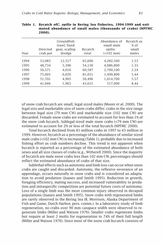
Crabs in Cold Water Regions: Biology, Management, and Economics 83
of snow crab bycatch are small, legal-sized males (Moore et al. 2000). Thelegal size and marketable size of snow crabs differ; crabs in the size rangebetween legal size (79 mm CW) and marketable size (102 mm CW) arediscarded. Female snow crabs are estimated to account for less than 1% ofthe snow crab bycatch. Sublegal-sized male snow crabs (<79 mm CW) areestimated to account for 2% or less of the total bycatch (NPFMC 2000).
Total bycatch declined from 81 million crabs in 1997 to 43 million in1999. However, bycatch as a percentage of the abundance of similar-sizedmale crabs (<102 mm CW) is increasing (Table 1), probably due to increasedfishing effort as crab numbers decline. This trend is not apparent whenbycatch is reported as a percentage of the estimated abundance of bothsexes and all size classes of crabs (e.g., Witherell 2000). Since the majorityof bycatch are male snow crabs less than 102 mm CW, percentages shouldreflect the estimated abundance of crabs of that size.
Sublethal effects such as autotomy and limb loss can occur when snowcrabs are caught and discarded. Autotomy, the reflexive severance of anappendage, occurs naturally in snow crabs and is considered an adapta-tion to avoid predation (Juanes and Smith 1995). Reduction in growth,foraging efficiency, mating success, and increased vulnerability to preda-tion and intraspecific competition are potential future costs of autotomy.Loss of a single limb was the most common injury observed in decapodpopulations (Juanes and Smith 1995). Snow crabs with regenerated limbsare rarely observed in the Bering Sea (R. Morrison, Alaska Department ofFish and Game, Dutch Harbor, pers. comm.). In a laboratory study of limbregeneration, no crabs over 90 mm carapace width were observed to re-generate limbs (Miller and Watson 1976). Smaller crabs regenerate limbsbut require at least 2 molts for regeneration to 74% of their full length(Miller and Watson 1976). Since most of the snow crab bycatch consists of
Table 1. Bycatch of C. opilio in Bering Sea fisheries, 1994-1999 and esti-mated abundance of small males (thousands of crabs) (NPFMC2000).
Groundfish Abundance of Bycatch as trawl, fixed small male % of
Directed gear, scallop Bycatch opilio smallYear crab pot dredge total (<102 mm) males
1994 53,083 12,517 65,600 4,282,500 1.53
1995 48,734 5,396 54,130 4,086,800 1.33
1996 56,571 4,016 60,587 2,700,100 2.24
1997 75,005 6,026 81,031 1,490,800 5.44
1998 51,591 4,905 56,496 1,014,700 5.57
1999 41,666 1,965 43,631 517,000 8.44
84 Warrenchuk and Shirley — Effects of Windchill
males larger than 90 mm, limb loss can be considered permanent. Injuryrates in the field were highly variable, but averaged 24% of discarded crabs(Tracey and Byersdorfer 2000).
Snow crabs of the size caught in the fishery may not regenerate limbsbecause the time and number of molts required is past terminal molt;molting rarely occurs beyond terminal molt. Tanner crabs, red king crabs,and American lobster (Homarus americanus) had a negative correlationbetween body size and injury (Juanes and Smith 1995). A negative correla-tion between body size and injury may indicate that injury reduces sur-vival, and fewer crabs with lost limbs survive to grow to a larger size.
The objectives of this study were to determine the effects of windchillexposure (cold air temperature and wind) on mortality, limb loss, andactivity (measured as a change in the righting response) for male snowcrabs (Chionoecetes opilio) of the size typically discarded as bycatch.
Materials and MethodsThis study was the first to use live C. opilio from the Bering Sea in a labo-ratory experiment. Male snow crabs of the size typically discarded by thefishery were collected (mean CW ± 1 S.D. = 96.3 mm ± 9.0 mm) from theBering Sea in April 2000. Crabs with bitter crab disease, black mat syn-drome, pepper crab, or torch disease (Jadamec et al. 1999) were not re-tained. Care was taken to minimize handling and exposure of the crabs toair. Crabs were maintained in flow-through seawater tanks at the JuneauCenter, School of Fisheries and Ocean Sciences and the National MarineFisheries Service, Auke Bay Laboratory. The seawater intake for both labsis at –30 m in Auke Bay; temperature and salinity variations were withinthe range recorded for the Bering Sea. Seawater discharge from the tankswas passed through a freshwater reservoir before being routed to the sea-water return line.
Crabs were observed for 2 weeks prior to initiation of the experimentto ensure health and uniformity. Size measurements, previous damage(old injuries), shell condition, and hemolymph screening for bitter crabdisease were performed on all specimens. Crabs were marked with Floytags attached with a plastic cable tie to the merus of the fourth or fifthpereiopod. After the completion of the study, the crabs were frozen anddisposed at the Alaska Department of Fish and Game tag lab.
The experiment was composed of seven experimental treatments andone control treatment with 15 replicate crabs in each treatment. Crabswere placed in tanks with one tank per treatment. Each treatment containeda sample of crab sizes with minimized variation in size between tanks.
Exposure times reflected actual sorting time measurements from thefield. Crabs were exposed to treatments for 5 minutes, similar to the aver-age maximum aerial exposure measured by observers in 1998 (Tracy andByersdorfer 2000). Total exposure time was reduced to 2.5 minutes fortwo of the most severe treatments.
Crabs in Cold Water Regions: Biology, Management, and Economics 85
Windchill TreatmentsWind and cold treatments were selected using the best available
weather data reflective of the Bering Sea during the crabbing season. Un-fortunately, the best weather data are obtained from a National WeatherService buoy 300 miles southwest of the fishing grounds. Weather at thebuoy and at the fishing grounds was assumed to be similar. Windchilltreatments were performed with the following combinations of wind speedand temperature for an exposure time of 5 minutes: –2ºC and 8 m persecond, –2ºC and 16 m per second, –6ºC and 8 m per second, –5ºC and 16m per second, –10ºC and 8 m per second, and a control with no exposure.The two most severe treatments, –5ºC and 16 m per second and –10ºC and8 m per second, were also performed with an exposure time of 2.5 minutes.
The windchill for each treatment was calculated using the NationalWeather Service formula:
Temp Temp Windspeed
Windspeed Temp Tempwindchill initial
air initial
= + ¥ ¥ +- ¥ ¥ -
0 045 5 27
10 45 0 28
. [( . )
. ( . )] ( )
where Windspeed = mean wind speed (km/hour), Tempair = ambient tem-perature (ºC), and Tempinitial = initial temperature of body (ºC). The initialbody temperature of a crab was assumed to be the same as the holdingwater temperature (~6ºC).
Windchill treatments were performed in a walk-in freezer. Tempera-ture was recorded every minute and averaged for the duration of the treat-ment. A squirrel cage blower was used to generate wind speeds through awind tunnel (44 ¥ 38 ¥ 239 cm) made of wood and plastic sheeting. Anelectronic anemometer measured wind speeds within the tunnel. To mini-mize aerial exposure, crabs were moved to the cold room while immersedin seawater. Crabs were placed inside the wind tunnel while confined withinmesh cages (43 ¥ 33 ¥ 23 cm, 2.5 ¥ 3.8 cm mesh) to insure uniformity ofexposure aspect. Immediately after exposure, crabs were replaced in sea-water and returned to the lab.
Observations of mortality, limb autotomy, and the righting responsewere made for each numbered crab immediately after crabs were returnedto the wet laboratory, then again after 24 hours, and after 7 days. Mortal-ity was determined by detection of movement of the scaphognathites (gillbailers), pereiopods, mandibles, and maxillae. Functional mortality, wherethe crab remained moribund for extended periods, was noted. Mortalitywas assessed daily for 7 days post-treatment and dead crabs were re-moved from the tanks. Crabs that survived treatments were used to testsignificance of autotomy and included in the analysis of righting response.The righting response is a complex reflex requiring muscle coordinationand balance and can be a sensitive measure of well-being of organisms(Shirley and Stickle 1982). Righting response was determined by placingthe crabs on their dorsum and measuring the time in seconds (to a maximum
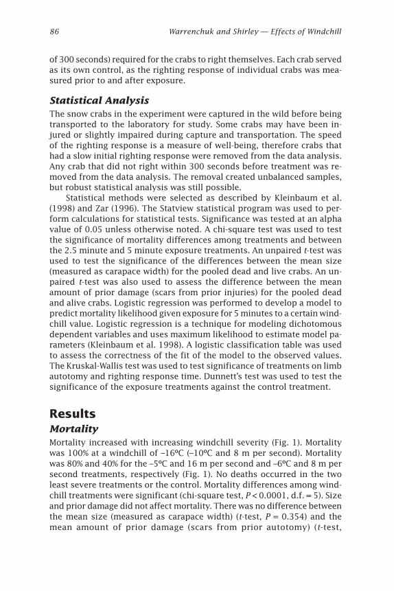
86 Warrenchuk and Shirley — Effects of Windchill
of 300 seconds) required for the crabs to right themselves. Each crab servedas its own control, as the righting response of individual crabs was mea-sured prior to and after exposure.
Statistical AnalysisThe snow crabs in the experiment were captured in the wild before beingtransported to the laboratory for study. Some crabs may have been in-jured or slightly impaired during capture and transportation. The speedof the righting response is a measure of well-being, therefore crabs thathad a slow initial righting response were removed from the data analysis.Any crab that did not right within 300 seconds before treatment was re-moved from the data analysis. The removal created unbalanced samples,but robust statistical analysis was still possible.
Statistical methods were selected as described by Kleinbaum et al.(1998) and Zar (1996). The Statview statistical program was used to per-form calculations for statistical tests. Significance was tested at an alphavalue of 0.05 unless otherwise noted. A chi-square test was used to testthe significance of mortality differences among treatments and betweenthe 2.5 minute and 5 minute exposure treatments. An unpaired t-test wasused to test the significance of the differences between the mean size(measured as carapace width) for the pooled dead and live crabs. An un-paired t-test was also used to assess the difference between the meanamount of prior damage (scars from prior injuries) for the pooled deadand alive crabs. Logistic regression was performed to develop a model topredict mortality likelihood given exposure for 5 minutes to a certain wind-chill value. Logistic regression is a technique for modeling dichotomousdependent variables and uses maximum likelihood to estimate model pa-rameters (Kleinbaum et al. 1998). A logistic classification table was usedto assess the correctness of the fit of the model to the observed values.The Kruskal-Wallis test was used to test significance of treatments on limbautotomy and righting response time. Dunnett’s test was used to test thesignificance of the exposure treatments against the control treatment.
ResultsMortalityMortality increased with increasing windchill severity (Fig. 1). Mortalitywas 100% at a windchill of –16ºC (–10ºC and 8 m per second). Mortalitywas 80% and 40% for the –5ºC and 16 m per second and –6ºC and 8 m persecond treatments, respectively (Fig. 1). No deaths occurred in the twoleast severe treatments or the control. Mortality differences among wind-chill treatments were significant (chi-square test, P < 0.0001, d.f. = 5). Sizeand prior damage did not affect mortality. There was no difference betweenthe mean size (measured as carapace width) (t-test, P = 0.354) and themean amount of prior damage (scars from prior autotomy) (t-test,
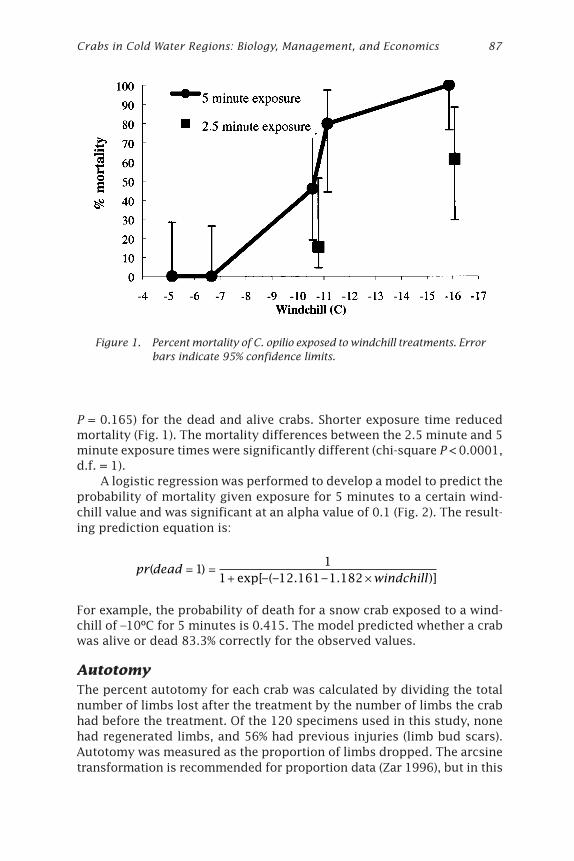
Crabs in Cold Water Regions: Biology, Management, and Economics 87
P = 0.165) for the dead and alive crabs. Shorter exposure time reducedmortality (Fig. 1). The mortality differences between the 2.5 minute and 5minute exposure times were significantly different (chi-square P < 0.0001,d.f. = 1).
A logistic regression was performed to develop a model to predict theprobability of mortality given exposure for 5 minutes to a certain wind-chill value and was significant at an alpha value of 0.1 (Fig. 2). The result-ing prediction equation is:
pr dead
windchill( )
exp[–(– . – . )]= =
+ ¥1
11 12 161 1 182
For example, the probability of death for a snow crab exposed to a wind-chill of –10ºC for 5 minutes is 0.415. The model predicted whether a crabwas alive or dead 83.3% correctly for the observed values.
AutotomyThe percent autotomy for each crab was calculated by dividing the totalnumber of limbs lost after the treatment by the number of limbs the crabhad before the treatment. Of the 120 specimens used in this study, nonehad regenerated limbs, and 56% had previous injuries (limb bud scars).Autotomy was measured as the proportion of limbs dropped. The arcsinetransformation is recommended for proportion data (Zar 1996), but in this
Figure 1. Percent mortality of C. opilio exposed to windchill treatments. Errorbars indicate 95% confidence limits.
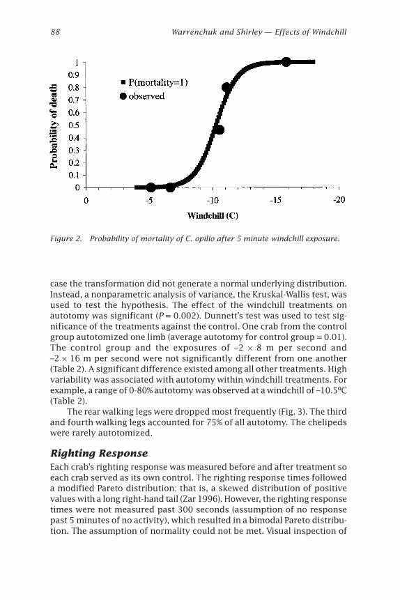
88 Warrenchuk and Shirley — Effects of Windchill
case the transformation did not generate a normal underlying distribution.Instead, a nonparametric analysis of variance, the Kruskal-Wallis test, wasused to test the hypothesis. The effect of the windchill treatments onautotomy was significant (P = 0.002). Dunnett’s test was used to test sig-nificance of the treatments against the control. One crab from the controlgroup autotomized one limb (average autotomy for control group = 0.01).The control group and the exposures of –2 ¥ 8 m per second and–2 ¥ 16 m per second were not significantly different from one another(Table 2). A significant difference existed among all other treatments. Highvariability was associated with autotomy within windchill treatments. Forexample, a range of 0-80% autotomy was observed at a windchill of –10.5ºC(Table 2).
The rear walking legs were dropped most frequently (Fig. 3). The thirdand fourth walking legs accounted for 75% of all autotomy. The chelipedswere rarely autotomized.
Righting ResponseEach crab’s righting response was measured before and after treatment soeach crab served as its own control. The righting response times followeda modified Pareto distribution; that is, a skewed distribution of positivevalues with a long right-hand tail (Zar 1996). However, the righting responsetimes were not measured past 300 seconds (assumption of no responsepast 5 minutes of no activity), which resulted in a bimodal Pareto distribu-tion. The assumption of normality could not be met. Visual inspection of
Figure 2. Probability of mortality of C. opilio after 5 minute windchill exposure.
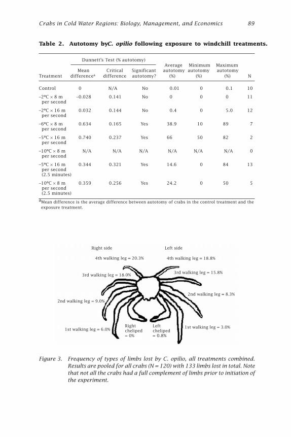
Crabs in Cold Water Regions: Biology, Management, and Economics 89
Table 2. Autotomy by C. opilio following exposure to windchill treatments.
Dunnett’s Test (% autotomy) Average Minimum Maximum
Mean Critical Significant autotomy autotomy autotomyTreatment differencea difference autotomy? (%) (%) (%) N
Control 0 N/A No 0.01 0 0.1 10
–2ºC ¥ 8 m –0.028 0.141 No 0 0 0 11 per second
–2ºC ¥ 16 m 0.032 0.144 No 0.4 0 5.0 12 per second
–6ºC ¥ 8 m 0.634 0.165 Yes 38.9 10 89 7 per second
–5ºC ¥ 16 m 0.740 0.237 Yes 66 50 82 2 per second
–10ºC ¥ 8 m N/A N/A N/A N/A N/A N/A 0 per second
–5ºC ¥ 16 m 0.344 0.321 Yes 14.6 0 84 13 per second (2.5 minutes)
–10ºC ¥ 8 m 0.359 0.256 Yes 24.2 0 50 5 per second (2.5 minutes)
aMean difference is the average difference between autotomy of crabs in the control treatment and the exposure treatment.
Figure 3. Frequency of types of limbs lost by C. opilio, all treatments combined.Results are pooled for all crabs (N = 120) with 133 limbs lost in total. Notethat not all the crabs had a full complement of limbs prior to initiation ofthe experiment.
90 Warrenchuk and Shirley — Effects of Windchill
the distribution of residuals also disproved the assumption ofhomoscedasticity. The lack of homoscedasticity is mainly a function ofthe response times that are truncated at 5 minutes. Therefore, the severetreatments in which all the crabs did not right themselves after 5 minuteshad lower variances than the control and the less severe treatments. Non-parametric analysis of the change in righting response was necessary. TheKruskal-Wallis test was used to test the effect of windchill treatment onthe righting response time. The change in response times due to treat-ment was significantly different (P = 0.002). Dunnett’s test (used for spe-cifically comparing controls to other treatments) (Zar 1996) did not showa significant difference between the control and the least severe windchilltreatment, but a significant difference did exist between the control andthe other three treatments (Table 3). Response times were either signifi-cantly slower or nonexistent. Response times were also significantly slowerafter the 2.5 minute exposure treatments. However, there was no signifi-cant difference between the response times from the 2.5 minute exposuretreatments and the 5 minute exposure treatments (Table 3).
DiscussionMortality increased with increasing severity of treatment. The probabilityof mortality increased after a windchill exposure of –10.3ºC for 5 minutes;no mortality occurred at less severe exposures. Death occurred even whena snow crab was exposed for 2.5 minutes at a windchill of –10.3ºC. Therapid cooling associated with windchill may cause some failure at thecellular level. Ice crystals forming in the cytoplasm disrupt cell membranesand cell death occurs. As heat loss approaches lethal limits, neurons arethe first cells to fail (Prosser 1991). Critical neuron failure is a probablecause of death. Body parts with high surface area to volume ratio areprobably the most susceptible to freezing damage. The appendages, eyestalks, and mouth parts could become irreversibly damaged and wouldcause impairment to the crab. The filamentous gills are also susceptible;injury to the gills could initiate mortality.
The mortality threshold between the –5ºC ¥ 16 m per second and–6ºC ¥ 8 m per second treatments may be due to the different wind speeds.High wind speed may increase the rate of water loss and evaporation fromthe gill chambers thereby increasing the potential for freezing damage tothe gills. The threshold response could be affected by many factors. Thetime of water retention in the gill chambers could have varied dependingupon the angle from which the crabs were removed from the water. Al-though size (measured as carapace width) and prior injuries were foundto be insignificant in predicting mortality, a larger sample size controlledfor these variables might have determined effects. However, the size rangeof crabs incidentally caught by the fishery is narrow so stratifying treat-ments by size may not be a useful endeavor.
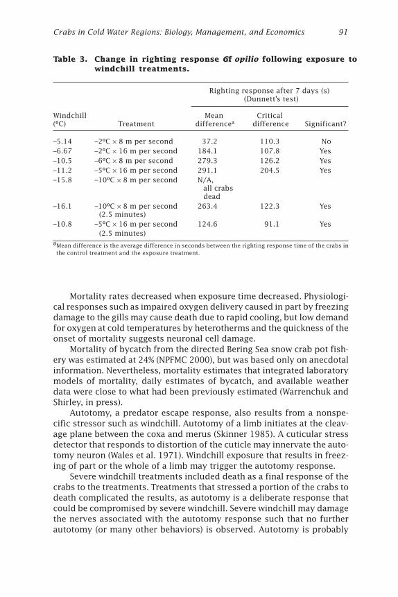
Crabs in Cold Water Regions: Biology, Management, and Economics 91
Mortality rates decreased when exposure time decreased. Physiologi-cal responses such as impaired oxygen delivery caused in part by freezingdamage to the gills may cause death due to rapid cooling, but low demandfor oxygen at cold temperatures by heterotherms and the quickness of theonset of mortality suggests neuronal cell damage.
Mortality of bycatch from the directed Bering Sea snow crab pot fish-ery was estimated at 24% (NPFMC 2000), but was based only on anecdotalinformation. Nevertheless, mortality estimates that integrated laboratorymodels of mortality, daily estimates of bycatch, and available weatherdata were close to what had been previously estimated (Warrenchuk andShirley, in press).
Autotomy, a predator escape response, also results from a nonspe-cific stressor such as windchill. Autotomy of a limb initiates at the cleav-age plane between the coxa and merus (Skinner 1985). A cuticular stressdetector that responds to distortion of the cuticle may innervate the auto-tomy neuron (Wales et al. 1971). Windchill exposure that results in freez-ing of part or the whole of a limb may trigger the autotomy response.
Severe windchill treatments included death as a final response of thecrabs to the treatments. Treatments that stressed a portion of the crabs todeath complicated the results, as autotomy is a deliberate response thatcould be compromised by severe windchill. Severe windchill may damagethe nerves associated with the autotomy response such that no furtherautotomy (or many other behaviors) is observed. Autotomy is probably
Table 3. Change in righting response of C. opilio following exposure towindchill treatments.
Righting response after 7 days (s) (Dunnett’s test)
Windchill Mean Critical(ºC) Treatment differencea difference Significant?
–5.14 –2ºC ¥ 8 m per second 37.2 110.3 No–6.67 –2ºC ¥ 16 m per second 184.1 107.8 Yes–10.5 –6ºC ¥ 8 m per second 279.3 126.2 Yes–11.2 –5ºC ¥ 16 m per second 291.1 204.5 Yes–15.8 –10ºC ¥ 8 m per second N/A,
all crabs dead
–16.1 –10ºC ¥ 8 m per second 263.4 122.3 Yes (2.5 minutes)
–10.8 –5ºC ¥ 16 m per second 124.6 91.1 Yes (2.5 minutes)
aMean difference is the average difference in seconds between the righting response time of the crabs in the control treatment and the exposure treatment.
92 Warrenchuk and Shirley — Effects of Windchill
maximized when the windchill exposure is severe enough to trigger thesynapse, but not so severe as to damage the nerves.
Autotomy resulting from windchill exposure differs from natural,predator-induced autotomy. Windchill-induced autotomy may be moresevere as multiple limbs can be lost following exposure. Windchill expo-sure is a nonspecific stressor whereas predator-induced autotomy is di-rected toward one or a few limbs. The stress of windchill exposure isanalogous to a predator that attacks every limb at the same time. Multiplelimb loss in populations of the related Tanner crab is rare (Juanes andSmith 1995), but sampling bias is probable.
The extent that appendage loss might affect an individual varies withthe number of damaged limbs. The loss of one walking leg would be ex-pected to have a minimal effect on crab fitness. However, the additiveeffects of many lost limbs and the pattern by which they are lost willaffect crab fitness. Autotomy does not necessarily preclude survival. Ashore crab, Hemigrapsus oregonensis, can survive over a year with no limbs(S.D. Rice, National Marine Fisheries Service, Auke Bay Laboratory, Juneau,unpubl. data). However, there is probably some level of autotomy thatmay affect survival. Snow crabs have 10 limbs: four pairs of walking legsand a pair of chelipeds. The chelipeds are presumably the most importantfor survival and function in feeding, defense, and mating (grasping offemales). Chelipeds were rarely lost as a result of windchill in our experi-ment. The rear (fourth) walking leg was the most readily autotomizedlimb, followed by any other walking leg. The rear walking legs may beimportant for some crab behaviors. When healthy crabs right themselvesafter being turned over, the most common technique involves a dorsal toventral flip from anterior to posterior. Snow crabs with a full number oflimbs use both rear (fourth) walking legs to first contact the substrate andinitiate the flip. The smaller diameter limbs may be more susceptible tofreezing damage and autotomy. Mathematical models have demonstratedthat the limbs may cool faster and reach a lower temperature than the crabbody (P. van Tamelen, Alaska Department of Fish and Game, pers. comm.).
Mating behaviors may be affected by autotomy. Tanner crab matingbehavior such as standing over a female, standing “high-on-legs,” kicking,and body lifting (of the female above the male) (Donaldson and Adams1989) rely on leverage and balance and may be difficult without a fullcomplement of limbs. These behaviors have also been observed duringantagonistic interactions with other males (Donaldson and Adams 1989).Autotomy could affect both mating behavior and competitive ability ofmale snow crabs.
Snow crabs in the laboratory flare out their limbs when grasped. It isa behavior that may stem from predator avoidance. A predator that seizesthe crab in the same fashion would be presented with a much larger effec-tive prey size and would have difficulty fitting the crab into its mouth. Acrab with fewer limbs would be easier to consume.
Crabs in Cold Water Regions: Biology, Management, and Economics 93
Injury rates of snow crabs aboard catcher-processors during the 1997-1998 Bering Sea snow crab fishery were assessed from 14,000 nonretainedsnow crabs from 394 sampled pots (Tracy and Byersdorfer 2000). Injuryrates varied among vessels from 7% to 44% of crabs sampled with an aver-age of 24%. Autotomized legs were the most prevalent injury and com-prised 59% of the total injuries. Major damage (cracked carapace, bent ortorn limbs, chela damage) composed 10.9% of the total injuries. Weatherconditions were not noted during the injury assessment sampling.
Injury rates from observer data are the rates of instantaneous limbloss that occurs over the few minutes that the crabs are held. Instanta-neous limb loss in the laboratory study occurred, but snow crabs alsoautotomized limbs over 7 days of observation. This suggests that esti-mates by observers of bycatch limb loss are conservative.
Annual pot surveys by observers on fishing vessels assess the crabcondition (and hence previous injuries). If the rate of limb loss in dis-carded crabs is high, this should be evident in pot samples as the crabsare captured again the following year. However, if injury and limb lossreduce survival, then estimates of bycatch limb loss will be conservative.
The snow crabs in this experiment were handled carefully after beingexposed to the windchill treatments. Bycatch snow crabs are not handledas gently on a fishing vessel, and any rough handling would exacerbatelimb loss.
The righting response was impaired in all but the least severe windchilltreatments. A threshold exists above a severity of exposure of –2ºC and 16m per second (~ –6ºC windchill) where the righting response is impaired.
A functional righting response depends on the unanimity of the ner-vous system and the musculature. The nervous system is complex andeven slight damage can result in a loss of function. Loss of coordinationwas evident by increased righting response times after red king crabs andTanner crabs were exposed to wind and cold (Shirley 1998, 1999). Snowcrabs exposed to windchill below –6ºC also had an impaired righting re-sponse. A snow crab with no righting response, in a state of chill coma,could be considered functionally dead.
Some red king crabs and Tanner crabs in a state of chill coma recov-ered seven days post exposure (Shirley 1999). In this study, several snowcrabs with no righting response immediately after the less severe treat-ments recovered after seven days post exposure, suggesting the potentialto recover from mild exposure. Snow crabs that survived severe to moder-ate windchill exposure were unlikely to recover.
Loss of mobility was evident after windchill exposure. Very little ac-tive movement was observed in crabs that survived windchill less than–10ºC. Only 4 of 8 surviving crabs from the –6ºC and 8 m per secondtreatment were observed actively moving. Sporadic motion of the limbswith no net movement described the remaining survivors. All crabs in theless severe windchill treatments actively moved, even when no righting
94 Warrenchuk and Shirley — Effects of Windchill
response was evident. Crabs that could move exhibited jerky, uncoordi-nated motion of the walking legs. High “standing-on-legs” travel was notnoted. Crab movement could be described as lifting the walking legs, push-ing and sliding the body across the substrate.
Impaired mobility could alter foraging efficiency, seasonal migration,and daily movement behaviors. However, little is known about movementpatterns of snow crabs in the Bering Sea. A tagging and recapture experi-ment in the Gulf of St. Lawrence found that snow crabs moved up to 3 kmin 48 hours (Brêthes et al. 1985).
Loss of mobility and coordination could make crabs more vulnerableto predation. Cod (Gadus morhua) prey seasonally on snow crab in thenorthwest Atlantic and can consume softshell males up to 110 mm CW(Robichaud et al. 1991). Heavy predation on Tanner and snow crabs oc-curs in the southeastern Bering Sea by Alaska and Bering skates, wattledeelpout, Pacific cod, and four sculpin species (Jewett 1982). Predation mightbe more severe if movement or escape responses of crabs were impaired.
It is ironic that the snow crab fishery itself, which catches the abun-dance of snow crab bycatch in the Bering Sea, is not constrained by anybycatch limits. The North Pacific Fishery Management Council could setlimits on the bycatch of snow crab using management similar to the ground-fish fisheries. The groundfish trawl fisheries are constrained by prohib-ited species catch (PSC) limits for snow crab. The snow crab PSC cap is setat 0.1133% of the Bering Sea stock abundance based on annual NationalMarine Fisheries Service trawl survey data, with a minimum PSC of 4.5million crabs and a maximum of 13 million snow crabs (NPFMC 2000).
Another option is to incorporate the estimated bycatch mortality inguideline harvest levels. However, with bycatch mortality included in har-vest limits, there would be no incentive for fishermen to release bycatchwith any concern for survival.
Ultimately, the fate of harvested snow crabs lies with the fishermen.They can choose whether or not to fish during extreme cold and severeweather. Deckhands could prioritize returning discarded crabs to the waterand do so as quickly as possible. Vessel owners can outfit their boats withslides or chutes to release bycatch as opposed to forcing crabs throughthe scuppers. In a fishery where the number of discarded crabs in one yearcan be higher than the allowable harvest the following year (i.e., in 1999-2000), ensuring the survival of discarded crabs makes good business sense.
AcknowledgmentsWe thank L. McNutt (University of Alaska Fairbanks) and Dr. A. Moles (Na-tional Marine Fisheries Service) for assistance. Our gratitude goes to person-nel in Dutch Harbor for support in snow crab collection: R. Morrison and staffat the Alaska Department of Fish and Game, L. Boyle and R. Burt from theObserver Training Center, and G. Blue and the crew of F/V Zolotoi. TheAuke Bay Laboratory graciously provided laboratory space and support. The
Crabs in Cold Water Regions: Biology, Management, and Economics 95
research was funded by the Alaska Department of Fish. and Game underCooperative Agreement NA97FN0129 from the National Oceanic and At-mospheric Administration (NOAA). The views expressed are those of the au-thors and do not necessarily reflect the views of NOAA or any of its subagencies.
ReferencesBrêthes, J.C., R. Bouchard, and G. Desrosiers. 1985. Determination of the area pros-
pected by a baited trap from a tagging and recapture experiment with snowcrabs (Chionoecetes opilio). J. Northw. Atl. Fish. Sci. 6:37-42.
Carls, M.G., and C.E. O’Clair. 1990. Influence of cold air exposures on ovigerous redking crabs (Paralithodes camtschatica) and Tanner crabs (Chionoecetes bairdi)and their offspring. In: Proceedings of the International Symposium on Kingand Tanner Crabs. University of Alaska Sea Grant, AK-SG-90-04, Fairbanks, pp.329-343.
Carls, M.G., and C.E. O’Clair. 1995. Responses of Tanner crabs, Chionoecetes bairdi,exposed to cold air. Fish. Bull., U.S. 93:44-56.
Court, A. 1948. Windchill. Bull. Am. Meteorology C. 29:487-493.
Donaldson, W.E., and A. Adams. 1989. Ethogram of behavior with emphasis onmating for the Tanner crab Chionoecetes bairdi Rathbun. J. Crustacean Biol.9:37-53.
Jadamec, L.K., W.E. Donaldson, and P. Cullenberg. 1999. Biological field techniquesfor Chionoecetes crabs. University of Alaska Sea Grant, AK-SG-99-02, Fairbanks.
Jewett, S.C. 1982. Predation on crabs of the genus Chionoecetes: Literature review.In: Proceedings of the International Symposium on the Genus Chionoecetes.University of Alaska Sea Grant, AK-SG-82-10, Fairbanks, pp. 521-539.
Juanes, F., and D. Smith. 1995. The ecological consequences of limb damage andloss in decapod crustaceans: A review and prospectus. J. Exp. Mar. Biol. Ecol.193:97-223.
Kleinbaum, D.G., L.L. Kupper, and K.E. Muller. 1998. Applied regression analysisand other multivariable methods, 3rd edition. Duxbury Press, Pacific Grove,California, pp. 656-686.
MacIntosh, R.A., B.G. Stevens, J.A. Haaga, and B.A. Johnson. 1996. Effects of han-dling and discarding mortality of Tanner crabs (Chionoecetes bairdi). In: Highlatitude crabs: Biology, management, and economics. University of Alaska SeaGrant, AK-SG-96-02, Fairbanks, pp. 591-611.
McLeese, D.W. 1968. Temperature resistance of the spider crab Chionoecetes opilio.J. Fish. Res. Board. Can. 25 (8):1733-1736.
Miller, R.J., and J. Watson. 1976. Growth per molt and limb regeneration in thespider crab, Chionoecetes opilio. J. Fish. Res. Board Can. 33:1644-1649.
Moore, H., L.C. Byrne, and D. Connolly. 2000. Alaska Department of Fish and Gamesummary of the 1998 mandatory shellfish observer program database. AlaskaDepartment of Fish and Game, Division of Commercial Fisheries, RegionalInformation Report 4K00-21, Kodiak.
96 Warrenchuk and Shirley — Effects of Windchill
North Pacific Fishery Management Council (NPFMC). 2000. Amendment 14 to theFishery Management Plan: A rebuilding plan for the Bering Sea C. opilio stock.National Marine Fisheries Service, Alaska Region, Sustainable Fisheries Divi-sion, P.O. Box 21668, Juneau, AK 99802.
Prosser, C.L. 1991. Environmental and metabolic animal physiology. John Wiley &Sons, pp. 115-130.
Robichaud, D.A., R.W. Elner, and R.F.J. Bailey. 1991. Differential selection of crabChionoecetes opilio and Hyas spp. as prey by sympatric cod Gadus morhuaand thorny skate Raja radiata. Fish. Bull., U.S. 89(4):669-679.
Shirley, T.C. 1998. Appendix D: Crab handling mortality and bycatch reduction. In:G.H. Kruse, King and Tanner crab research in Alaska: Annual report for July 1,1997 to June 30, 1998. Alaska Department of Fish and Game, Division of Com-mercial Fisheries, Regional Information Report 5J98-07, Juneau.
Shirley, T.C. 1999. Appendix B: Effects of windchill on red king crabs. In: G.H. Kruse(ed.), King and Tanner crab research in Alaska: Annual report for July 1, 1998through June 30, 1999. Alaska Department of Fish and Game, Division of Com-mercial Fisheries, Regional Information Report 5J99-10, Juneau.
Shirley, T.C., and W.B. Stickle. 1982. Responses of Leptasterias hexactis (Echinoder-mata: Asteroidea) to low salinity. I. Survival, activity, feeding, growth and ab-sorption efficiency. Mar. Biol. 169:147-154.
Skinner, D.M. 1985. Molting and regeneration. In: D.E. Bliss and L.H. Mantel (eds.),Biology of Crustacea, vol. 9. Academic Press, New York, pp. 43-146.
Tracy, D., and S.C. Byersdorfer. 2000. Summary of crab injury assessment and aeri-al exposure sample results from selected 1997/1998 Bering Sea/Aleutian Is-lands king and Tanner crab fisheries and the 1998 Pribilof Islands hair crabfishery. Alaska Department of Fish and Game, Division of Commercial Fisher-ies, Regional Information Report 4K00-52, Kodiak.
Wales, W., F. Clarac, and M.S. Laverack. 1971. Stress detection at the autotomyplane in the decapod Crustacea. I. Comparative anatomy of the receptors ofthe basi-ischiopodite. Z. Vgl. Physiol. 73:357-382.
Warrenchuk, J.J., and T.C. Shirley. 2002. Estimates of mortality of snow crabs, Chio-noecetes opilio, discarded during the Bering Sea fishery in 1998. Alaska Fish.Res. Bull. 9(1).
Witherell, D. 2000. BSAI crab bycatch. In: Crab Plan Team. Stock assessment andfishery evaluation report for the king and Tanner crab fisheries of the BeringSea and Aleutian Islands regions. North Pacific Fishery Management Council,Anchorage, Alaska.
Zar, J.H. 1996. Biostatistical analysis. Prentice-Hall, Upper Saddle River, New Jer-sey. 649 pp.
Zhou, S., and T.C. Shirley. 1995. Effects of handling on feeding, activity, and surviv-al of red king crabs, Paralithodes camtschaticus (Tilesius, 1815). J. ShellfishRes. 14(1):173-177.
Crabs in Cold Water Regions: Biology, Management, and Economics 97Alaska Sea Grant College Program • AK-SG-02-01, 2002
Testing CarapaceMorphology Characteristicsfor Field Identification ofChionoecetes HybridsDaniel Urban and Douglas PengillyAlaska Department of Fish and Game, Kodiak, Alaska
Luke JadamecUniversity of Maine, Orono, Maine
Susan C. ByersdorferAlaska Department of Fish and Game, Kodiak, Alaska
AbstractThe ability of Tanner crabs, Chionoecetes bairdi, and snow crabs, C. opilio,to hybridize in the Bering Sea was first recorded in 1969 and biologistssince then have struggled with the identification of the various forms ofthe hybrids. The hybrids are not uniformly intermediate between the pa-rental types, but form a smooth cline of morphological types making thefield identification of hybrids a difficult and subjective task. Over 1,000genetically typed carapaces were examined in an effort to develop an ac-curate field identification technique for hybrids and their parental spe-cies. An ordinal scoring system was developed for six morphologicalcharacters with scores ranging from 1 for C. bairdi to 5 for C. opilio, withhybrids being intermediate. Photographs of character variation by crabtype are presented. A classification tree and discriminant function analy-sis were applied to learning sets of carapace scores, and then to test sets,but neither technique could reliably identify carapaces when applied todata outside of the individual learning and test sets. The scoring systemdeveloped here can be used with good success for developing a classifica-tion scheme for a single scorer, but inconsistency of scorers, as demon-strated by components of variance analysis, proved an impediment todeveloping a broadly applicable scheme.
98 Urban et al. — Carapace Morphology Characteristics
IntroductionTanner crabs, Chionoecetes bairdi, and snow crabs, C. opilio, are both widelydistributed in the North Pacific Ocean and Bering Sea, with the snow crabhaving a more northerly distribution that extends to the Arctic Ocean.Snow crabs also occur in the northwest Atlantic Ocean (Fig. 1). Hybrids ofTanner crabs and snow crabs were first recognized by their intermediatemorphological characters in 1969 (Karinen and Hoopes 1971) in an area ofdistributional overlap in the eastern Bering Sea (Fig. 1). The hybridizationwas later confirmed through the use of protein electrophoresis by Johnson(1976) and expanded upon by Grant et al. (1978) and Merkouris et al.(1998). Hybrids in general do not present a single phenotype, but rather awide range of types intermediate to the two parental species. In addition,the gradation is typically not uniform for all characters, but forms a mo-saic of types (Barton and Hewitt 1985). The Chionoecetes hybrids followthis pattern. There is also evidence that these hybrids are fertile and willproduce an F2 generation or may backcross with the parental species(Merkouris et al. 1998). The F2 and backcross hybrids have proven difficultto distinguish from the parental species using either genetic or morpho-logical methods (Campton 1987).
The intermediacy of hybrid morphological characters and their gra-dation into those of the parent stocks pose problems in the field identifi-cation of Chionoecetes in the eastern Bering Sea. Chionoecetes bairdi andC. opilio have both supported valuable commercial fisheries in the easternBering Sea, and those identification problems have resulted in problemsfor fisheries management. During the 1990 commercial fishery for C. opilioin the Bering Sea, for example, concerns were raised due to sublegal C. bairdibeing landed as “hybrids” (ADFG 1991). Those concerns were complicatedby legal questions on identification of C. bairdi, C. opilio, and hybrid crabsduring commercial fisheries and on the legality of retaining hybrids dur-ing the C. bairdi and C. opilio commercial fisheries. In 1991 the AlaskaBoard of Fisheries resolved those legal questions by adopting a regulatorydefinition of C. bairdi and C. opilio (5 AAC 35.521; ADFG 1992) that wasintended to minimize commercial landings of C. bairdi as hybrids or C.opilio. Under that legal definition, C. bairdi are identified on the basis ofeye color and epistome characteristics; all C. bairdi, C. opilio, and hybridsnot conforming to those characteristics are legally considered C. opilio.
Although the legal definition has apparently been effective in the pur-pose for which it was developed, it provides no means for distinguishinghybrids from C. bairdi or C. opilio, which is still an important need forfisheries management and assessing population trends. For example, ac-curate assessment of bycatch during commercial fisheries is hamperedby the difficulty in reliably identifying the three crab types that can occuras bycatch. The potential errors can be great. Using the C. opilio fishery in1997 as an example, it was estimated by the Alaska Department of Fishand Game (ADFG) that the bycatch of C. bairdi was 4.52 million, but the
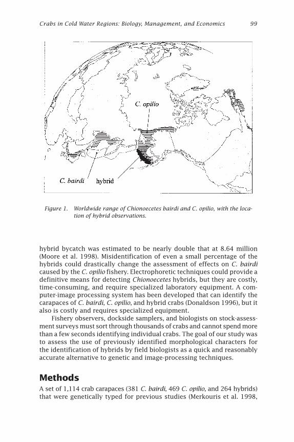
Crabs in Cold Water Regions: Biology, Management, and Economics 99
hybrid bycatch was estimated to be nearly double that at 8.64 million(Moore et al. 1998). Misidentification of even a small percentage of thehybrids could drastically change the assessment of effects on C. bairdicaused by the C. opilio fishery. Electrophoretic techniques could provide adefinitive means for detecting Chionoecetes hybrids, but they are costly,time-consuming, and require specialized laboratory equipment. A com-puter-image processing system has been developed that can identify thecarapaces of C. bairdi, C. opilio, and hybrid crabs (Donaldson 1996), but italso is costly and requires specialized equipment.
Fishery observers, dockside samplers, and biologists on stock-assess-ment surveys must sort through thousands of crabs and cannot spend morethan a few seconds identifying individual crabs. The goal of our study wasto assess the use of previously identified morphological characters forthe identification of hybrids by field biologists as a quick and reasonablyaccurate alternative to genetic and image-processing techniques.
MethodsA set of 1,114 crab carapaces (381 C. bairdi, 469 C. opilio, and 264 hybrids)that were genetically typed for previous studies (Merkouris et al. 1998,
Figure 1. Worldwide range of Chionoecetes bairdi and C. opilio, with the loca-tion of hybrid observations.
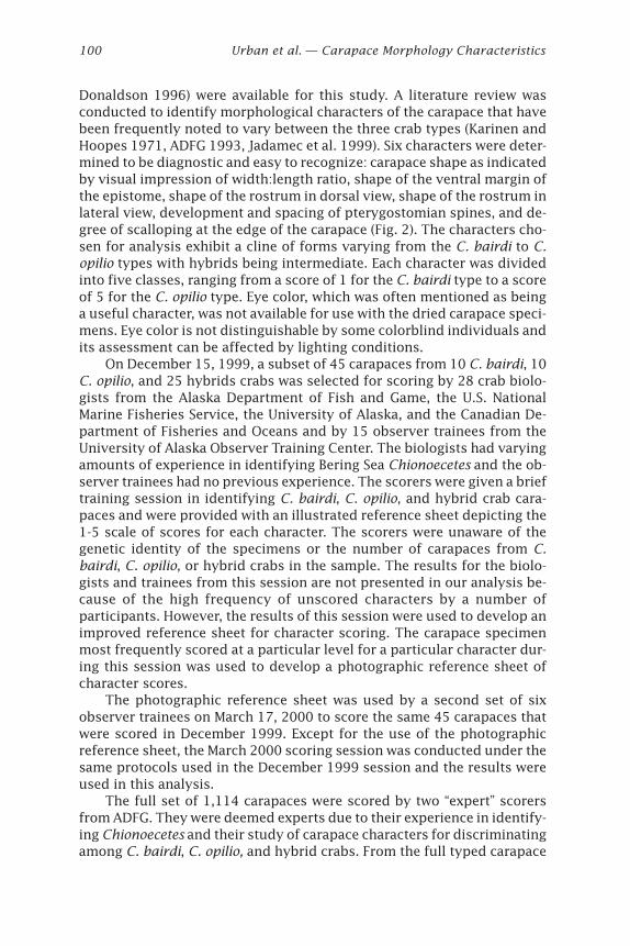
100 Urban et al. — Carapace Morphology Characteristics
Donaldson 1996) were available for this study. A literature review wasconducted to identify morphological characters of the carapace that havebeen frequently noted to vary between the three crab types (Karinen andHoopes 1971, ADFG 1993, Jadamec et al. 1999). Six characters were deter-mined to be diagnostic and easy to recognize: carapace shape as indicatedby visual impression of width:length ratio, shape of the ventral margin ofthe epistome, shape of the rostrum in dorsal view, shape of the rostrum inlateral view, development and spacing of pterygostomian spines, and de-gree of scalloping at the edge of the carapace (Fig. 2). The characters cho-sen for analysis exhibit a cline of forms varying from the C. bairdi to C.opilio types with hybrids being intermediate. Each character was dividedinto five classes, ranging from a score of 1 for the C. bairdi type to a scoreof 5 for the C. opilio type. Eye color, which was often mentioned as beinga useful character, was not available for use with the dried carapace speci-mens. Eye color is not distinguishable by some colorblind individuals andits assessment can be affected by lighting conditions.
On December 15, 1999, a subset of 45 carapaces from 10 C. bairdi, 10C. opilio, and 25 hybrids crabs was selected for scoring by 28 crab biolo-gists from the Alaska Department of Fish and Game, the U.S. NationalMarine Fisheries Service, the University of Alaska, and the Canadian De-partment of Fisheries and Oceans and by 15 observer trainees from theUniversity of Alaska Observer Training Center. The biologists had varyingamounts of experience in identifying Bering Sea Chionoecetes and the ob-server trainees had no previous experience. The scorers were given a brieftraining session in identifying C. bairdi, C. opilio, and hybrid crab cara-paces and were provided with an illustrated reference sheet depicting the1-5 scale of scores for each character. The scorers were unaware of thegenetic identity of the specimens or the number of carapaces from C.bairdi, C. opilio, or hybrid crabs in the sample. The results for the biolo-gists and trainees from this session are not presented in our analysis be-cause of the high frequency of unscored characters by a number ofparticipants. However, the results of this session were used to develop animproved reference sheet for character scoring. The carapace specimenmost frequently scored at a particular level for a particular character dur-ing this session was used to develop a photographic reference sheet ofcharacter scores.
The photographic reference sheet was used by a second set of sixobserver trainees on March 17, 2000 to score the same 45 carapaces thatwere scored in December 1999. Except for the use of the photographicreference sheet, the March 2000 scoring session was conducted under thesame protocols used in the December 1999 session and the results wereused in this analysis.
The full set of 1,114 carapaces were scored by two “expert” scorersfrom ADFG. They were deemed experts due to their experience in identify-ing Chionoecetes and their study of carapace characters for discriminatingamong C. bairdi, C. opilio, and hybrid crabs. From the full typed carapace
Crabs in Cold Water Regions: Biology, Management, and Economics 101
set (not including the 45 that had been scored earlier by observer train-ees), 250 carapaces of each type were randomly chosen for analysis. Eachof the samples of 250 carapaces from the three genetic types was ran-domly subsampled to produce a “learning set” of 600 carapaces (200 fromeach genetic type) and a “test set” of 150 carapaces. The two experts alsorescored five times each a randomly chosen subset of 100 carapaces com-posed of 28 C. bairdi, 34 C. opilio, and 28 hybrid crabs.
A number of statistical techniques were used to analyze the observertrainee and expert carapace scores. Discriminant function analysis (DFA),which has historically been used when a group of specimens from eachcategory is known (Neff and Smith 1979), was used to determine the char-acters that were most important for discriminating between groups. WhileDFA may provide insights into the importance of the variables, the resultscan be difficult to interpret and utilize in a field situation. Classificationtree algorithms (Breiman et al. 1984) were applied to the data sets as theywere seen as being a useful tool in a field situation for distinguishing crabtypes. Classification trees have become a popular alternative to DFA andother multivariate procedures. Classification tree algorithms are appliedto the data as a directed graphing technique where each split in a data setis used to decrease the “impurity” of the data with the final nodes reflect-ing the desired classification categories. Stopping criteria are key to thefunctioning of the classification tree procedure; without them each final
Figure 2. Characters used to distinguish Tanner crab, snow crab, and their hy-brids.
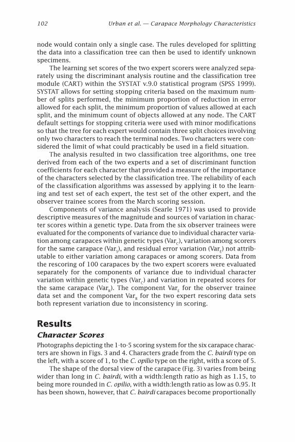
102 Urban et al. — Carapace Morphology Characteristics
node would contain only a single case. The rules developed for splittingthe data into a classification tree can then be used to identify unknownspecimens.
The learning set scores of the two expert scorers were analyzed sepa-rately using the discriminant analysis routine and the classification treemodule (CART) within the SYSTAT v.9.0 statistical program (SPSS 1999).SYSTAT allows for setting stopping criteria based on the maximum num-ber of splits performed, the minimum proportion of reduction in errorallowed for each split, the minimum proportion of values allowed at eachsplit, and the minimum count of objects allowed at any node. The CARTdefault settings for stopping criteria were used with minor modificationsso that the tree for each expert would contain three split choices involvingonly two characters to reach the terminal nodes. Two characters were con-sidered the limit of what could practicably be used in a field situation.
The analysis resulted in two classification tree algorithms, one treederived from each of the two experts and a set of discriminant functioncoefficients for each character that provided a measure of the importanceof the characters selected by the classification tree. The reliability of eachof the classification algorithms was assessed by applying it to the learn-ing and test set of each expert, the test set of the other expert, and theobserver trainee scores from the March scoring session.
Components of variance analysis (Searle 1971) was used to providedescriptive measures of the magnitude and sources of variation in charac-ter scores within a genetic type. Data from the six observer trainees wereevaluated for the components of variance due to individual character varia-tion among carapaces within genetic types (VarC), variation among scorersfor the same carapace (VarS), and residual error variation (VarE) not attrib-utable to either variation among carapaces or among scorers. Data fromthe rescoring of 100 carapaces by the two expert scorers were evaluatedseparately for the components of variance due to individual charactervariation within genetic types (VarC) and variation in repeated scores forthe same carapace (VarR). The component VarE for the observer traineedata set and the component VarR for the two expert rescoring data setsboth represent variation due to inconsistency in scoring.
ResultsCharacter ScoresPhotographs depicting the 1-to-5 scoring system for the six carapace charac-ters are shown in Figs. 3 and 4. Characters grade from the C. bairdi type onthe left, with a score of 1, to the C. opilio type on the right, with a score of 5.
The shape of the dorsal view of the carapace (Fig. 3) varies from beingwider than long in C. bairdi, with a width:length ratio as high as 1.15, tobeing more rounded in C. opilio, with a width:length ratio as low as 0.95. Ithas been shown, however, that C. bairdi carapaces become proportionally
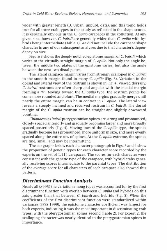
Crabs in Cold Water Regions: Biology, Management, and Economics 103
wider with greater length (D. Urban, unpubl. data), and this trend holdstrue for all three crab types in this study as reflected in the shape scores.It is especially obvious in the C. opilio carapaces in the collection. At anygiven size, however, C. bairdi are generally wider than C. opilio with hy-brids being intermediate (Table 1). We did not include the carapace shapecharacter in any of our subsequent analyses due to that character’s depen-dency on size.
Figure 3 shows the deeply notched epistome margin of C. bairdi, whichvaries to the virtually straight margin of C. opilio. Not only the angle be-tween the middle two plates of the epistome varies, but also the anglebetween the next two distal plates.
The lateral carapace margin varies from strongly scalloped in C. bairdito the smooth margin found in many C. opilio (Fig. 3). Variation in thedorsal and lateral view of the rostrum is shown in Fig. 4. Viewed dorsally,C. bairdi rostrums are often sharp and angular with the medial marginforming a “V”. Moving toward the C. opilio type, the rostrum points be-come more rounded and blunt. The medial margins gradually merge untilnearly the entire margin can be in contact in C. opilio. The lateral viewreveals a steeply inclined and recurved rostrum in C. bairdi. The dorsalmargin of the C. opilio rostrum can be straight and slightly downwardpointing.
Chionoecetes bairdi pterygostomian spines are strong and pronounced,closely spaced anteriorly and gradually becoming larger and more broadlyspaced posteriorly (Fig. 4). Moving toward the C. opilio type, the spinesgradually become less pronounced, more uniform in size, and more evenlyspaced along the entire row of spines. At the C. opilio extreme, the spinesare fine, small, and may be intermittent.
The bar graphs below each character photograph in Figs. 3 and 4 showthe proportion of genetic types for each character score recorded by theexperts on the set of 1,114 carapaces. The scores for each character wereconsistent with the genetic type of the carapace, with hybrid crabs gener-ally receiving scores intermediate to the parental types. The distributionof the average score for all characters of each carapace also showed thispattern.
Discriminant Function AnalysisNearly all (>99%) the variation among types was accounted for by the firstdiscriminant function with overlap between C. opilio and hybrids on thisaxis greater than that between C. bairdi and hybrids (Fig. 5). When thecoefficients of the first discriminant function were standardized withinvariances (SPSS 1999), the epistome character coefficient was largest forboth experts, indicating it was the most important in discriminating crabtypes, with the pterygostomian spines second (Table 2). For Expert 2, thescalloping character was nearly identical to the pterygostomian spines inimportance.
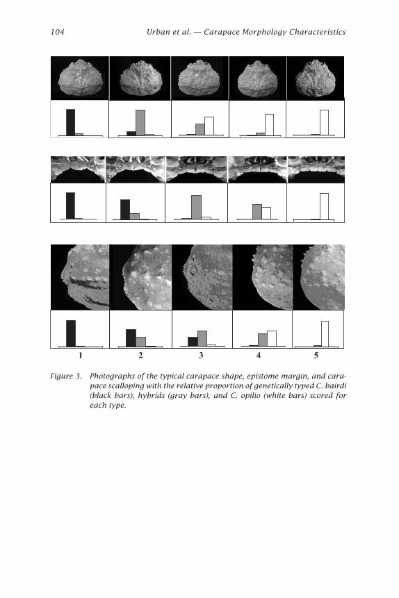
104 Urban et al. — Carapace Morphology Characteristics
Figure 3. Photographs of the typical carapace shape, epistome margin, and cara-pace scalloping with the relative proportion of genetically typed C. bairdi(black bars), hybrids (gray bars), and C. opilio (white bars) scored foreach type.
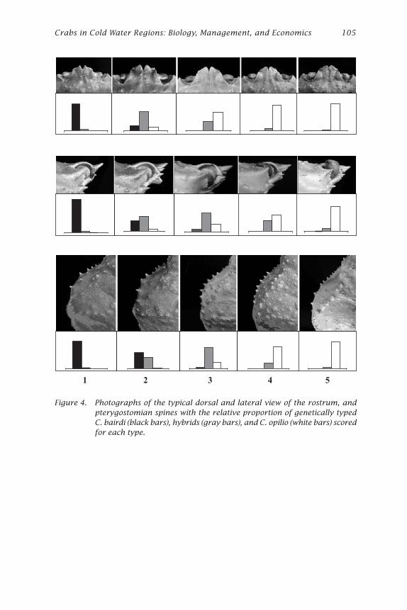
Crabs in Cold Water Regions: Biology, Management, and Economics 105
1 2 3 4 5
Figure 4. Photographs of the typical dorsal and lateral view of the rostrum, andpterygostomian spines with the relative proportion of genetically typedC. bairdi (black bars), hybrids (gray bars), and C. opilio (white bars) scoredfor each type.
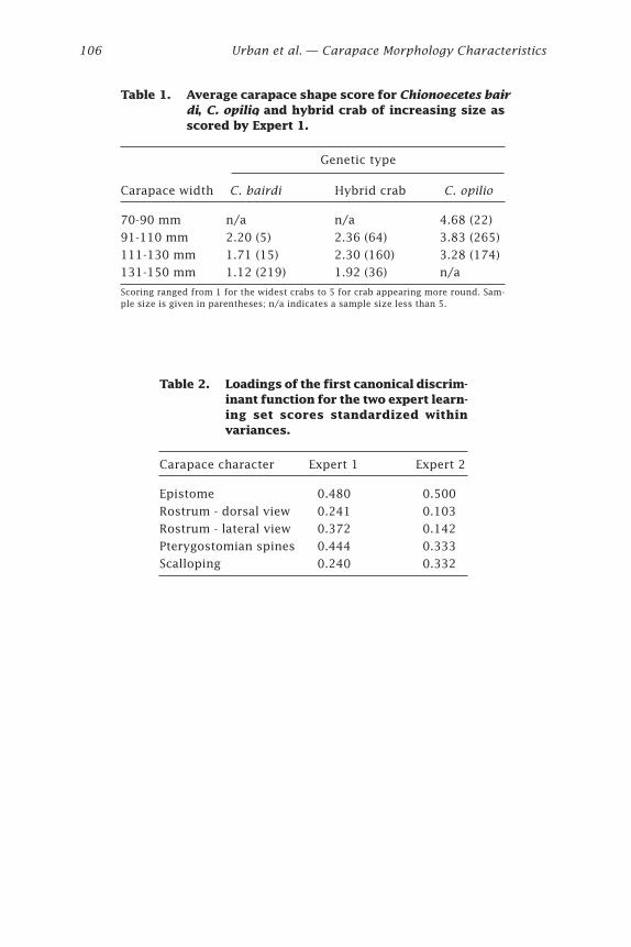
106 Urban et al. — Carapace Morphology Characteristics
Table 1. Average carapace shape score for Chionoecetes bair-di, C. opilio, and hybrid crab of increasing size asscored by Expert 1.
Genetic type
Carapace width C. bairdi Hybrid crab C. opilio
70-90 mm n/a n/a 4.68 (22)
91-110 mm 2.20 (5) 2.36 (64) 3.83 (265)
111-130 mm 1.71 (15) 2.30 (160) 3.28 (174)
131-150 mm 1.12 (219) 1.92 (36) n/a
Scoring ranged from 1 for the widest crabs to 5 for crab appearing more round. Sam-ple size is given in parentheses; n/a indicates a sample size less than 5.
Table 2. Loadings of the first canonical discrim-inant function for the two expert learn-ing set scores standardized withinvariances.
Carapace character Expert 1 Expert 2
Epistome 0.480 0.500
Rostrum - dorsal view 0.241 0.103
Rostrum - lateral view 0.372 0.142
Pterygostomian spines 0.444 0.333
Scalloping 0.240 0.332
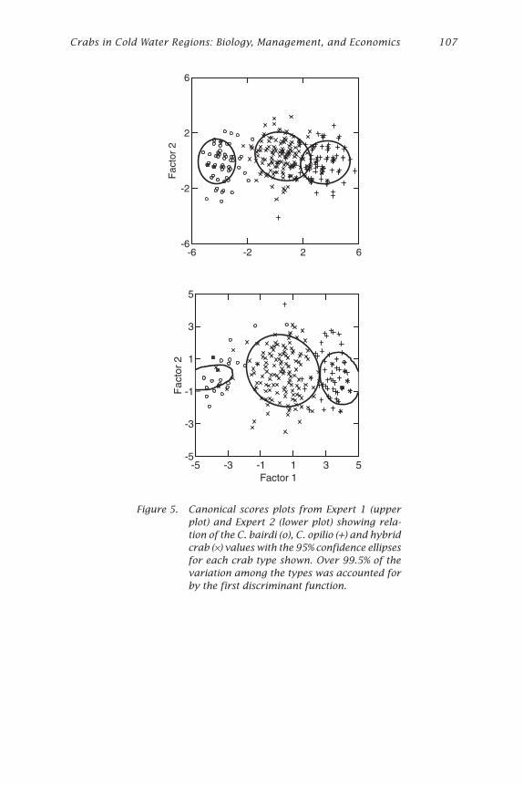
Crabs in Cold Water Regions: Biology, Management, and Economics 107
Figure 5. Canonical scores plots from Expert 1 (upperplot) and Expert 2 (lower plot) showing rela-tion of the C. bairdi (o), C. opilio (+) and hybridcrab (¥) values with the 95% confidence ellipsesfor each crab type shown. Over 99.5% of thevariation among the types was accounted forby the first discriminant function.
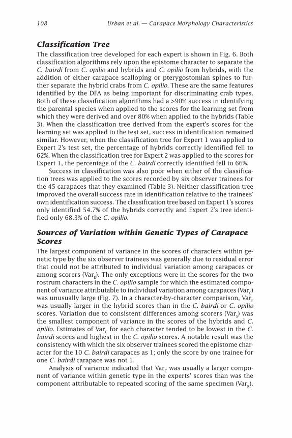
108 Urban et al. — Carapace Morphology Characteristics
Classification TreeThe classification tree developed for each expert is shown in Fig. 6. Bothclassification algorithms rely upon the epistome character to separate theC. bairdi from C. opilio and hybrids and C. opilio from hybrids, with theaddition of either carapace scalloping or pterygostomian spines to fur-ther separate the hybrid crabs from C. opilio. These are the same featuresidentified by the DFA as being important for discriminating crab types.Both of these classification algorithms had a >90% success in identifyingthe parental species when applied to the scores for the learning set fromwhich they were derived and over 80% when applied to the hybrids (Table3). When the classification tree derived from the expert’s scores for thelearning set was applied to the test set, success in identification remainedsimilar. However, when the classification tree for Expert 1 was applied toExpert 2’s test set, the percentage of hybrids correctly identified fell to62%. When the classification tree for Expert 2 was applied to the scores forExpert 1, the percentage of the C. bairdi correctly identified fell to 66%.
Success in classification was also poor when either of the classifica-tion trees was applied to the scores recorded by six observer trainees forthe 45 carapaces that they examined (Table 3). Neither classification treeimproved the overall success rate in identification relative to the trainees’own identification success. The classification tree based on Expert 1’s scoresonly identified 54.7% of the hybrids correctly and Expert 2’s tree identi-fied only 68.3% of the C. opilio.
Sources of Variation within Genetic Types of CarapaceScoresThe largest component of variance in the scores of characters within ge-netic type by the six observer trainees was generally due to residual errorthat could not be attributed to individual variation among carapaces oramong scorers (VarE). The only exceptions were in the scores for the tworostrum characters in the C. opilio sample for which the estimated compo-nent of variance attributable to individual variation among carapaces (VarC)was unusually large (Fig. 7). In a character-by-character comparison, VarE
was usually larger in the hybrid scores than in the C. bairdi or C. opilioscores. Variation due to consistent differences among scorers (VarS) wasthe smallest component of variance in the scores of the hybrids and C.opilio. Estimates of VarC for each character tended to be lowest in the C.bairdi scores and highest in the C. opilio scores. A notable result was theconsistency with which the six observer trainees scored the epistome char-acter for the 10 C. bairdi carapaces as 1; only the score by one trainee forone C. bairdi carapace was not 1.
Analysis of variance indicated that VarC was usually a larger compo-nent of variance within genetic type in the experts’ scores than was thecomponent attributable to repeated scoring of the same specimen (VarR).
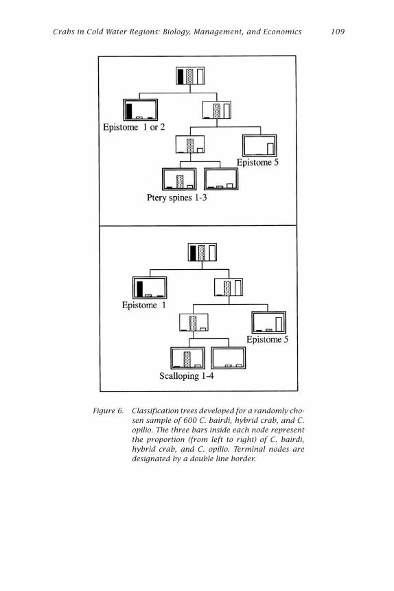
Crabs in Cold Water Regions: Biology, Management, and Economics 109
Figure 6. Classification trees developed for a randomly cho-sen sample of 600 C. bairdi, hybrid crab, and C.opilio. The three bars inside each node representthe proportion (from left to right) of C. bairdi,hybrid crab, and C. opilio. Terminal nodes aredesignated by a double line border.
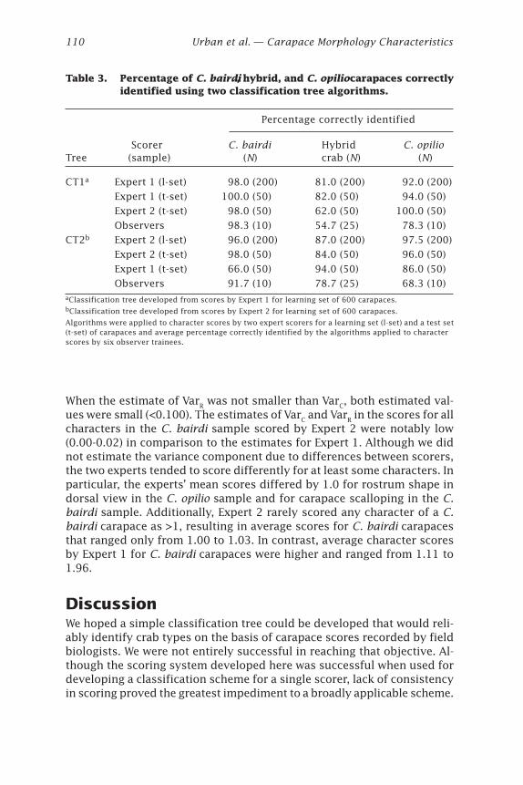
110 Urban et al. — Carapace Morphology Characteristics
When the estimate of VarR was not smaller than VarC, both estimated val-ues were small (<0.100). The estimates of VarC and VarR in the scores for allcharacters in the C. bairdi sample scored by Expert 2 were notably low(0.00-0.02) in comparison to the estimates for Expert 1. Although we didnot estimate the variance component due to differences between scorers,the two experts tended to score differently for at least some characters. Inparticular, the experts’ mean scores differed by 1.0 for rostrum shape indorsal view in the C. opilio sample and for carapace scalloping in the C.bairdi sample. Additionally, Expert 2 rarely scored any character of a C.bairdi carapace as >1, resulting in average scores for C. bairdi carapacesthat ranged only from 1.00 to 1.03. In contrast, average character scoresby Expert 1 for C. bairdi carapaces were higher and ranged from 1.11 to1.96.
DiscussionWe hoped a simple classification tree could be developed that would reli-ably identify crab types on the basis of carapace scores recorded by fieldbiologists. We were not entirely successful in reaching that objective. Al-though the scoring system developed here was successful when used fordeveloping a classification scheme for a single scorer, lack of consistencyin scoring proved the greatest impediment to a broadly applicable scheme.
Table 3. Percentage of C. bairdi, hybrid, and C. opilio carapaces correctlyidentified using two classification tree algorithms.
Percentage correctly identified
Scorer C. bairdi Hybrid C. opilioTree (sample) (N) crab (N) (N)
CT1a Expert 1 (l-set) 98.0 (200) 81.0 (200) 92.0 (200)
Expert 1 (t-set) 100.0 (50) 82.0 (50) 94.0 (50)
Expert 2 (t-set) 98.0 (50) 62.0 (50) 100.0 (50)
Observers 98.3 (10) 54.7 (25) 78.3 (10)
CT2b Expert 2 (l-set) 96.0 (200) 87.0 (200) 97.5 (200)
Expert 2 (t-set) 98.0 (50) 84.0 (50) 96.0 (50)
Expert 1 (t-set) 66.0 (50) 94.0 (50) 86.0 (50)
Observers 91.7 (10) 78.7 (25) 68.3 (10)aClassification tree developed from scores by Expert 1 for learning set of 600 carapaces.bClassification tree developed from scores by Expert 2 for learning set of 600 carapaces.
Algorithms were applied to character scores by two expert scorers for a learning set (l-set) and a test set(t-set) of carapaces and average percentage correctly identified by the algorithms applied to characterscores by six observer trainees.
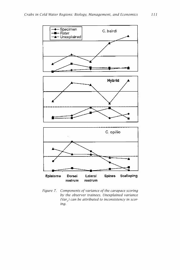
Crabs in Cold Water Regions: Biology, Management, and Economics 111
Figure 7. Components of variance of the carapace scoringby the observer trainees. Unexplained variance(VarE ) can be attributed to inconsistency in scor-ing.
112 Urban et al. — Carapace Morphology Characteristics
Several examples illustrate that point. Expert 2 gave nearly all theepistomes of C. bairdi carapaces a score of 1, which is reflected in thatexpert’s classification tree. However, when Expert 2’s classification treewas applied to Expert 1’s more variable C. bairdi epistome scoring, it per-formed poorly. Similarly, Expert 1’s tree had very poor success in identify-ing hybrid crabs when applied to the observer trainees’ scores. That poorsuccess can be explained by the high VarE (0.816) in the scores of thetrainee observers for the pterygostomian spines character, the characterthat Expert 1’s tree relied on to identify the hybrid crabs.
The greatest component of variance in character scores by traineeobservers was due to inconsistent scoring of carapaces (i.e., poor repeatabil-ity). Character variation within types and consistent scoring differencesamong novices were lesser components of variance. That suggests moretraining is needed if character scoring by novice field biologists is to beused in identifying types through a classification algorithm.
The results of the expert scorers indicated that they were consistentin repeated scores for the same carapace. A greater problem is that theexperts may not be consistent with each other in interpreting a characterscoring. Each expert seems to have developed their own concept of thecrab types and they rely on it more heavily than a reference score sheet,first generally recognizing the carapaces by gestalt. This gestalt sublimi-nally seems to influence their scoring of characters. Again, this suggeststhe need for greater objectivity if character scoring is to be used in identi-fying types through a classification algorithm. The photographic scoringguide developed for this project will, we hope, assist in reaching this goal.
ReferencesADFG (Alaska Department of Fish and Game). 1991. Westward Region report to the
Alaska Board of Fisheries, March 1991. Alaska Department of Fish and Game,Division of Commercial Fisheries, Regional Information Report 4K91-4, Kodiak.
ADFG (Alaska Department of Fish and Game). 1992. Commercial shellfish regula-tions, 1992 edn. Alaska Department of Fish and Game, Division of CommercialFisheries, Juneau.
ADFG (Alaska Department of Fish and Game). 1993. ADFG observer manual forAlaskan crab processors, 3rd edn. Dutch Harbor, Alaska.
Barton, N.H., and G.M. Hewitt. 1985. Analysis of hybrid zones. Annu. Rev. Ecol.Syst. 16:113-148.
Breiman, L., J.H. Friedman, R.A. Olshen, and C.I. Stone. 1984. Classification andregression trees. Wadsworth, Belmont, California.
Campton, D.E. 1987. Natural hybridization and introgression in fishes: Methods ofdetection and genetic interpretations. In: N. Ryman and F. Utter (eds.), Popula-tion genetics and fishery management. University of Washington, Seattle, pp.161-192.
Crabs in Cold Water Regions: Biology, Management, and Economics 113
Donaldson, W.E. 1996. Development of an expert computer vision-based crab clas-sification system. In: High latitude crabs: Biology, management, and econom-ics. University of Alaska Sea Grant, AK-SG-96-02, Fairbanks, pp. 99-114.
Grant, W.S., L. Bartlett, and F.M. Utter. 1978. Biochemical genetic identification ofspecies and hybrids of the Bering Sea Tanner crab, Chionoecetes bairdi and C.opilio. Proc. Natl. Shellfish Assoc. 68:127.
Jadamec, L.S., W.E. Donaldson, and P.J. Cullenberg. 1999. Biological field techniquesfor Chionoecetes crabs. University of Alaska Sea Grant, AK-SG-99-02, Fairbanks,80 pp.
Johnson, A.G. 1976. Electrophoretic evidence of hybrid snow crab, Chionoecetesbairdi ¥ opilio. Fish. Bull., U.S. 74:693-694.
Karinen, J.F., and D.T. Hoopes. 1971. Occurrence of Tanner crabs (Chionoecetes sp.)in the eastern Bering Sea with characteristics intermediate between C. bairdiand C. opilio. Proc. Natl. Shellfish Assoc. 61:8-9.
Merkouris, S.E., L.W. Seeb, and M.C. Murphy. 1998. Low levels of genetic diversityin highly exploited populations of Alaskan Tanner crabs, Chionoecetes bairdi,and Alaskan and Atlantic snow crabs, C. opilio. Fish. Bull., U.S. 96:525-537.
Moore, H., L.C. Byrne, and D. Connolly. 1998. Alaska Department of Fish and Gamesummary of the 1997 mandatory observer program database. Alaska Depart-ment of Fish and Game, Division of Commercial Fisheries, Regional Informa-tion Report 4K98-50, Kodiak.
Neff, N.A., and G.R. Smith. 1979. Multivariate analysis of hybrid fishes. Syst. Zool.25:176-196.
Searle, S.R. 1971. Linear models. John Wiley, New York.
SPSS. 1999. SYSTAT 9. SPSS, Inc., Chicago.
.
