critical knowledge gaps: estimating potential maximum
TRANSCRIPT

Critical knowledge gaps: estimating potential maximum cumulative anthropogenic mortality limits
of key marine mammal species to inform management
Alice I. Mackay, Simon D. Goldsworthy and Peter Harrison
August 2016
FRDC Project No. 2015/035

1
© Year Fisheries Research and Development Corporation and South Australian Research and Development Institute. All rights reserved.
ISBN 978-1-921563-91-1
Critical knowledge gaps: estimating potential maximum cumulative anthropogenic mortality limits of key marine mammal species to inform management.
2015/035
2016
Ownership of Intellectual property rights Unless otherwise noted, copyright (and any other intellectual property rights, if any) in this publication is owned by the Fisheries Research and Development Corporation and the South Australian Research and Development Institute. This work is copyright. Apart from any use as permitted under the Copyright Act 1968 (Cth), no part may be reproduced by any process, electronic or otherwise, without the specific written permission of the copyright owner. Neither may information be stored electronically in any form whatsoever without such permission.
This publication (and any information sourced from it) should be attributed to Mackay, A.I., Goldsworthy, S.D. and Harrison, S. South Australian Research and Development Institute (Aquatic Sciences) 2016, Critical knowledge gaps: estimating potential maximum cumulative anthropogenic mortality limits of key marine mammal species to inform management. Adelaide, 2016.
Creative Commons licence All material in this publication is licensed under a Creative Commons Attribution 3.0 Australia Licence, save for content supplied by third parties, logos and the Commonwealth Coat of Arms.
Creative Commons Attribution 3.0 Australia Licence is a standard form licence agreement that allows you to copy, distribute, transmit and adapt this publication provided you attribute the work. A summary of the licence terms is available from creativecommons.org/licenses/by/3.0/au/deed.en. The full licence terms are available from creativecommons.org/licenses/by/3.0/au/legalcode.
Inquiries regarding the licence and any use of this document should be sent to: [email protected]
Disclaimer The authors warrant that they have taken all reasonable care in producing this report. The report has been through the SARDI internal review process, and has been formally approved for release by the Research Chief, Aquatic Sciences. Although all reasonable efforts have been made to ensure quality, SARDI does not warrant that the information in this report is free from errors or omissions. SARDI does not accept any liability for the contents of this report or for any consequences arising from its use or any reliance placed upon it. Material presented in these Administrative Reports may later be published in formal peer-reviewed scientific literature.
The information, opinions and advice contained in this document may not relate, or be relevant, to a readers particular circumstances. Opinions expressed by the authors are the individual opinions expressed by those persons and are not necessarily those of the publisher, research provider or the FRDC.
The Fisheries Research and Development Corporation plans, invests in and manages fisheries research and development throughout Australia. It is a statutory authority within the portfolio of the federal Minister for Agriculture, Fisheries and Forestry, jointly funded by the Australian Government and the fishing industry.
Researcher Contact Details FRDC Contact Details
Name:
Address:
Phone:
Fax:
Email:
A.I. Mackay
c/o SARDI Aquatic Sciences, 2 Hamra Ave, West Beach, SA 5024
08 8207 5400
08 8207 5481
Address:
Phone:
Fax:
Email: Web:
25 Geils Court
Deakin ACT 2600
02 6285 0400
02 6285 0499
www.frdc.com.au
In submitting this report, the researcher has agreed to FRDC publishing this material in its edited form.

2
Contents
Contents .................................................................................................................................................. 2
Acknowledgments .................................................................................................................................. 4
Abbreviations ......................................................................................................................................... 5
Executive Summary ............................................................................................................................... 6
Introduction ............................................................................................................................................ 8
Objectives ............................................................................................................................................. 14
Methods ................................................................................................................................................ 14
Stakeholder workshop ..................................................................................................................... 14
Closed technical workshop and expert elicitation ........................................................................... 15
Potential Biological Removal analysis ............................................................................................ 15
Estimates of Nmin used in PBR calculations .............................................................................. 17 Australian sea lions (ASL): ...................................................................................................... 17 Long-nosed fur seals (LNFS): .................................................................................................. 18 Australian fur seals (AUFS): .................................................................................................... 19 Short beaked common dolphins (SBCD): ................................................................................ 21 Tursiops spp.: ............................................................................................................................ 22
Results ................................................................................................................................................... 23
PBR Analysis ............................................................................................................................ 23
Discussion ............................................................................................................................................. 27
Conclusion ............................................................................................................................................ 38
Recommendations ................................................................................................................................ 40
References ............................................................................................................................................. 41
Appendix A............................................................................................................................................47
3
Tables
Table 1: Values and data sources used to calculate Potential Biological Removal (PBR) limits for
Australian sea lions. .................................................................................................................................. 18 Table 2: Values and data sources used to calculate Potential Biological Removal (PBR) limits for long-
nosed fur seals. .......................................................................................................................................... 19 Table 3: Values and data sources used to calculate Potential Biological Removal (PBR) limits for
Australian fur seals. .................................................................................................................................. 20 Table 4: Values and data sources used to calculate Potential Biological Removal (PBR) limits for short
beaked common dolphin in Management Zone 3. .................................................................................... 22 Table 5a. Potential Biological Removal (PBR) values for cumulative annual anthropogenic mortalities
of Australian sea lions (ALS) in Zone 1 of the SPF management area. Nmin was calculated using the
most recent pup estimates for that colony and a pup multiplier of 3.8. Sources of pup estimates are
Dennis and Shaughnessy 19961, Gales et al. 19942 and the Department of Parks and Wildlife, Western
Australia3. Rmax is the maximum growth rate, FR is the recovery factor (range 0.1-0.4). ......................... 23 Table 5b. Potential Biological Removal (PBR) values for cumulative annual anthropogenic mortalities
of Australian sea lions (ASL) in Zone 2 in the SPF management area. Nmin was calculated using colony
pup production estimates in Goldsworthy et al. (2015a) and a pup multiplier of 3.8. Rmax is the maximum
growth rate, FR is the recovery factor (range 0.1-0.4). .............................................................................. 24 Table 6. Potential Biological Removal (PBR) values for cumulative annual anthropogenic mortalities of
long-nosed fur seals (LNFS) in three proposed zones in the SPF management area. Nmin from expert
elicitation represent the group average lowest plausible and group average best estimates of abundance.
Rmax is the maximum growth rate, FR is the recovery factor (range 0.5-1). .............................................. 25 Table 7. Potential Biological Removal (PBR) values for cumulative annual anthropogenic mortalities of
Australian fur seals (AUFS) in in the SPF management area. Nmin is the minimum abundance estimate,
Rmax is the maximum growth rate, Fr is the recovery factor. .................................................................... 25 Table 8. Potential Biological Removal (PBR) values for cumulative annual anthropogenic mortalities of
short beaked common dolphins (SBCD) considering abundance estimates from state waters of the Gulfs
and / or on shelf-waters <100m depth within Zone 3 of the SPF bycatch management area. .................. 26 Table 9. Potential Biological Removal (PBR) values for cumulative annual anthropogenic mortalities for
populations of coastal bottlenose dolphins (Tursiops species) based on published estimates of
abundance. ................................................................................................................................................ 26
Figures
Figure 1: The two management zones considered by participants during the second round of Expert
Elicitation when providing estimates of Australian sea lion abundance. These management zones reflect
those used by AFMA under the Australian sea lion management strategy. ............................................. 17 Figure 2: The three spatial management zones considered by participants during the second round of
Expert Elicitation when providing estimates of long-nosed fur seal abundance. AFMA does not use
spatial management zones for interactions between Commonwealth fisheries and fur seals. .................. 18 Figure 3: The single management zone considered by participants during the second round of Expert
Elicitation when providing estimates of Australian fur seal abundance. AFMA does not use spatial
management zones for interactions between Commonwealth fisheries and fur seals. ............................. 20 Figure 4: The seven management zones considered by participants during the second round of Expert
Elicitation when providing estimates of short-beaked common dolphin abundance. These seven
management zones are used by AFMA to manage dolphin interactions within the SPF. ........................ 21 Figure 5: Range of assessment approaches and data requirements of bycatch management under the
Bycatch Policy and Harvest Strategy Policy. ERM= ecological risk management; HS= harvest strategy;
SAFE = Sustainability Assessment for Fishing Effects; SICA = Scale Intensity Consequence Analysis.
Source: Penney et al. (2013). .................................................................................................................... 35

4
Acknowledgments
This project was funded by the Fisheries Research and Development Corporation (FRDC). The editors
would like to thank the participants of the stakeholder and Closed Technical Workshop (CTW) for their
time and input into the project.
We would particularly like to acknowledge and thank all the participants of the CTW for valued
discussions during the workshop and constructive comments on earlier drafts of those reports. We also
thank all those who prepared and provided presentations during the stakeholder workshop. Thank you also
to Dr Jan Carey from the Centre of Excellence for Biosecurity Risk Analysis (CEBRA) for conducting
the Expert Elicitation (EE) process as part of the CTW.
Sarah-Lena Reinhold (SARDI) provided valuable support with workshop logistics and as rapporteur
during both workshops.
We thank Dr Lachlan McLeay and Dr Paul Rogers at SARDI Aquatic Sciences for their comments and
review of the report. The report was approved for release by A/Prof Jason Tanner, Subprogram Leader –
Environmental Assessment, Mitigation and Rehabilitation, Marine Ecosystems, SARDI Aquatic Sciences.

5
Abbreviations
AFMA – Australian Fisheries Management Authority
ASL – Australian sea lion
AUFS – Australian fur seal
CoP – Code of Practice
CTW – Closed technical workshop
DAFF – Department of Agriculture, Fisheries and Forestry
EE – Expert Elicitation
ERAEF – Ecological Risk Assessment of the Effects of Fishing
EM – Electronic monitoring
ERM – Ecological Risk Management
ETBF – Eastern Tuna and Billfish Fishery
ETP – Eastern Tropical Pacific
GHAT - Gillnet Hook and Trap sector
HS – Harvest strategy
HSP – Harvest Strategy Policy
LNFS – long-nosed fur seal (formerly New Zealand fur seal)
MMED – Marine Mammal Excluder Device
MMPA – United States Marine Mammal Protection Act
MU – Management Unit
NMFS – National Marine Fisheries Service
OSP -Optimum Sustainable Population
PBR – Potential Biological Removal
PSA – Productivity Susceptibility Analysis
PVA – Population Viability Analyses
SAFE – Sustainability Assessment for Fishing Effects
SARs – Stock Assessment Reports
SBCD – short-beaked common dolphin
SICA – Scale Intensity Consequence Analysis
SPF – Commonwealth Small Pelagic Fishery
SESSF – Commonwealth Southern and Eastern Scalefish and Shark Fishery
SET – South East Trawl sector of the SESSF
TAP – Threat Abatement Plan
TEPS – Threatened, Endangered, Protected Species
VMP – Vessel Management Plan
WTBF – Western Tuna and Billfish Fishery
ZMRG – Zero Mortality Rate Goal
6
Executive Summary
The Commonwealth Small Pelagic Fishery (SPF) has attracted significant public attention as a result of
marine mammal bycatch mortalities (common dolphins and fur seals) in mid-water trawl operations by
the FV Geelong Star since it commenced fishing in April 2015. The Australian Fisheries Management
Authority (AFMA) currently has a number of management measures in place to minimise further
interactions between marine mammals and the fishery that include spatial and temporal closures based on
bycatch trigger limits. However, the method by which trigger limits are developed for different species is
unclear. As a result a two day workshop organised by the Fisheries Research and Development
Corporation (FRDC) in Melbourne, Victoria, on 25-26 June 2015 recommended that “An expert group
should be established to review current information available to inform the establishment of trigger limits
for key marine mammal species (especially the short-beaked common dolphin, Australian fur seals and
long-nosed fur seals)” (Fitzgerald et al. 2015).
To directly address the recommendations of Fitzgerald et al. (2015) a two day workshop was convened at
SARDI Aquatic Sciences, Adelaide on 19- 20 October 2015, chaired by Professor Peter Harrison, Director
of the Marine Ecology Research Centre, Southern Cross University. The first day of the workshop aimed
to provide stakeholders from Commonwealth and State fisheries and environment agencies, industry and
eNGOs with a summary of currently available information on the abundance and distribution of key
marine mammal species in the area of the SPF. On the second day, a closed technical workshop (CTW)
was convened of invited scientists from government or universities who were directly involved in the
collection or analysis of abundance or distribution data and/or had demonstrated expertise in research
relating to marine mammal ecology.
To meet the recommendation of Fitzgerald et al. (2015), the current project investigated if Potential
Biological Removal (PBR) could be calculated for key marine mammal populations that overlap with the
fishing area of the SPF to inform the setting of bycatch trigger limits. In US managed fisheries, PBR, is
used to estimate limits to bycatch of marine mammal populations. The calculation of PBR requires a recent
estimate of abundance for the population considered. Recent abundance estimates for the three pinniped
species (Australian sea lion, Australian fur seals and long-nosed fur seals) were available for most of their
range overlapping with the SPF. Abundance estimates for short-beaked common dolphins were only
available for a small area that overlaps with the SPF and not available for offshore areas. Abundance
estimates for bottlenose dolphin species were only available for a small number of discrete coastal areas
and lacking for offshore areas. Invited experts discussed these data and undertook expert elicitation (EE)
to estimate abundance of these species in relation to spatial management zones in the SPF. Workshop
participants did not support EE as a means to estimate marine mammal abundance where no data were
available. The number of participants who provided estimates when published estimates were available
varied by species and/or management zone. The CTW provided a synthesis of available information on
the abundance and distribution of key marine mammal species and highlighted existing gaps in
information on these species.
After completion of the CTW and EE process, preliminary PBR was estimated for the Australian sea lion,
Australian fur seal, long-nosed fur seal, and short-beaked common dolphin for those geographical areas
of the SPF area where EE estimates were based on available abundance data. The project did not consider
other methods to estimate limits to bycatch mortality. Although PBR provides a relatively straightforward
means of calculating limits to anthropogenic mortality the method requires regularly updated estimates of
population abundance and bycatch removal across all fisheries and jurisdictions for that population.
AFMA apply bycatch trigger limits for specified marine mammal species/taxa in the midwater trawl sector
of the SPF and gillnet sector of the Commonwealth Southern and Eastern Scalefish and Shark Fishery
(SESSF). These limits are used in conjunction with additional management strategies such as spatial

7
closures and vessel specific management plans.. Trigger limits for Australian sea lion are set based on
information on population abundance and sub-structuring. In the absence of such data for other marine
mammal species, AFMA have selected conservative fishery or taxa specific trigger limits.
There remains a need to develop performance measures and decision rules to manage bycatch of protected
species in Australian commercial fisheries. There is also a need to develop transparent bycatch reference
points (both trigger and limit) and consider the cumulative impact on populations for high risk species
across Commonwealth and State fisheries. Current fishery specific marine mammal risk assessments
undertaken through the Ecological Risk Assessment of the Effects of Fishing (ERAEF) process, could be
improved by including quantitative data on bycatch and monitoring levels across fisheries and
jurisdictions, and should include a spatial bycatch risk analysis based on the temporal distribution of
fishing effort and distribution and relative density of the bycatch species.
Future setting of fishery specific marine mammal trigger limits should follow a risk assessment approach
that considers the impact of cumulative bycatch across fisheries and jurisdictions. A framework to
determine trigger limits for a population based on relative risk posed by different fisheries could be
implemented to ensure trigger limits reflect assessed levels of bycatch risk. Trigger limits could then be
used as performance indicators within fishery specific bycatch management plans such as those used by
AFMA.

8
Introduction
The management of bycatch in Australian Commonwealth waters is legislated under the Fisheries
Management Act 1991 (FM Act), and the Environment Protection and Biodiversity Conservation Act 1999
(EPBC Act). All marine mammal species are listed under the EPBC Act. The Commonwealth Policy on
Fisheries Bycatch (2000) was recently reviewed (DAFF 2013). The review recommended that bycatch
species should be assessed and managed according to both the level of interaction(s) and the level of
understanding and impact risk from that level of interaction. The less information there is on the extent or
effect of interactions on a species, the more precautionary the assessment and management of these
interactions should be. The review identified the use of quantitative decision rules and reference points as
a method for managing interactions with high risk species that could be consistently applied across
fisheries and species (DAFF 2013).
Based on the definitions of the Food and Agriculture Organization of the United Nations (FAO), this
report considers two types of fisheries management reference points; Target Reference Points and Limit
Reference Points (Caddy & Mahon 1995). Target Reference Points (TRPs) are defined as indicating ‘to a
state of a fishing and/or resource which is considered to be desirable and at which management action,
whether during development or stock rebuilding, should aim.’
Limit Reference Points (LRPs) are defined as indicating ‘a state of a fishery and/or a resource which is
considered to be undesirable and which management action should avoid.’ The Potential Biological
Removal (PBR), is an estimate of the upper limit to the cumulative anthropogenic mortality that a
population can sustain and can be considered an LRP. However, this LRP does not imply that this entire
limit should be reached.
Bycatch management in Australian Commonwealth fisheries
The Australian Fisheries Management Authority (AFMA) manages and mitigates bycatch of Threatened,
Endangered and Protected (TEP) species through fishery-specific bycatch and discarding workplans
(AFMA 2008) or under Threat Abatement Plans (TAP) for seabirds (Commonwealth of Australia 2014).
Examples of species specific bycatch strategies include the Dolphin Strategy and Australian Sea Lion
Management Strategy (AFMA 2010b) in the Gillnet, Hook and Trap sector of the Commonwealth
Southern and Eastern Scalefish and Shark Fishery (SESSF). Fishery specific risks to TEP species are
assessed using the Ecological Risk Assessment of the Effects of Fishing (ERAEF) process which uses a
tiered hierarchical framework to assess the risk that a specified fishery management objective is not
achieved (Hobday et al. 2007, 2011). Five ecological components are evaluated using a three tier process,
with the data requirements for risk assessments increasing from largely qualitative (Level 1) to
quantitative (Level 3). One of the specified components of the ERAEF is an assessment of the impacts of
fishing on TEP species. The ERAEF process aims to identify risks at Level 1, which can then be assessed
through a semi-quantitative approach at Level 2 and a quantitative approach at Level 3. The identification
of TEP species assessed as being of high or medium residual risk is used to prioritise management actions
under fishery-specific bycatch and discarding workplans (e.g. AFMA 2014a). These can include the use
of bycatch mitigation devices e.g. marine mammal excluder devices (MMEDs), Codes of Practice (CoP),
specified levels of observer coverage, and species-specific bycatch limits that trigger management actions
including temporal and spatial closures (e.g. AFMA 2014a). AFMA is currently revising its ERAEF
methodology and is conducting trials of that methodology in a number of fisheries, including the SPF
(AFMA pers. comm.).
9
These species specific trigger limits function in such a way that when a certain level of bycatch is reached
or exceeded, an immediate management action is triggered. Trigger limits for the management of dolphin
and seal interactions are currently in place in the gillnet sector of the SESSF and Small Pelagic Fishery
(SPF) (AFMA 2010b, 2014b). Bycatch trigger limits for marine mammals within these fisheries have been
set at either the individual vessel or fleet level, with the objective of reducing bycatch to as close to zero
as possible. Trigger limits result in the temporary cessation of fishing and/or the temporal closure of
fishing areas for a specified period of time.
Bycatch trigger limits for Australian sea lion (ASL) (Neophoca cinerea) in the Gillnet Hook and Trap
(GHAT) sector of the SESSF are specified under the Australian Sea Lion Management Strategy (AFMA
2010b). Current ASL bycatch trigger limits are for seven spatial zones that are based on information
regarding population structuring, size of breeding colonies and number of colonies (AFMA 2010b).
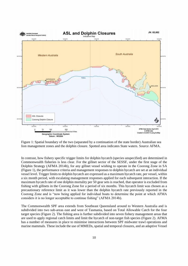
Permanent spatial closures are in place around breeding sites (Figure 1), and additional closures are
triggered if the ASL bycatch limit within a zone is reached. Current management arrangements assume
that individual colonies represent subpopulations and include having larger permanent closures around
colonies that were assessed to have a “higher predicted risk of fishery bycatch, low pup production and
terminal extinction risk” than other colonies. The design of spatial closures and the setting of trigger limits
were based on the results of Population Viability Analyses (PVAs), that assessed the impact of bycatch
mortality on the projected population status of ASL colonies in both South Australia (SA) (Goldsworthy
et al. 2010) and Western Australia (WA) (Campbell 2011). While initially applied to the SESSF, these
spatial closures and ASL management zones are also mandatory for the SPF.
10
Figure 1: Spatial boundary of the two (separated by a continuation of the state border) Australian sea
lion management zones and the dolphin closure. Spotted area indicates State waters. Source AFMA.
In contrast, how fishery specific trigger limits for dolphin bycatch (species unspecified) are determined in
Commonwealth fisheries is less clear. For the gillnet sector of the SESSF, under the first stage of the
Dolphin Strategy (AFMA 2014b), for any gillnet vessel wishing to operate in the Coorong Zone in SA
(Figure 1), the performance criteria and management responses to dolphin bycatch are set at an individual
vessel level. Trigger limits to dolphin bycatch are expressed as a maximum bycatch rate, per vessel, within
a six month period, with escalating management responses applied for each subsequent interaction. If the
maximum bycatch rate of one dolphin mortality per 50 gear sets is reached, that operator is excluded from
fishing with gillnets in the Coorong Zone for a period of six months. This bycatch limit was chosen as a
precautionary reference limit as it was lower than the dolphin bycatch rate previously reported in the
Coorong Zone and is “now being applied for individual boats to determine the point at which AFMA
considers it is no longer acceptable to continue fishing” (AFMA 2014b).
The Commonwealth SPF area extends from Southeast Queensland around to Western Australia and is
subdivided into two sub-areas east and west of Tasmania, based on Total Allowable Catch for the four
target species (Figure 2). The fishing area is further subdivided into seven fishery management areas that
are used to apply regional catch limits and limit the bycatch of non-target fish species (Figure 2). AFMA
has a number of measures in place to minimise interactions between SPF midwater trawl operations and
marine mammals. These include the use of MMEDs, spatial and temporal closures, and an adaptive Vessel
11
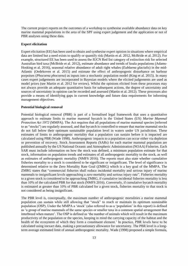
Management Plan (VMP) that specifies mandatory operational procedures and the use of approved
mitigation measures (AFMA 2015a).
The results of ERAEF for midwater trawl operations in the SPF identified 23 marine mammal species as
high risk using Productivity Susceptibility Analysis (PSA) (Daley et al. 2007). The residual risk analysis
of the Level 2 PSA, which takes into consideration management measures in the fishery, retained eight of
these species as high risk (AFMA 2010a). These were the Australian fur seal (Arctocephalus pusiilus
doriferus), bottlenose dolphin (Tursiops truncatus), Indian Ocean bottlenose dolphin (Tursiops aduncus),
Fraser’s dolphin (Lagenodelphis hosei), hourglass dolphin (Lagenorhynchus cruciger), Risso’s dolphin
(Grampus griseus), southern right whale dolphin (Lissodelphis peronii) and the striped dolphin (Stenella
coeruleoalba). The short-beaked common dolphin (SBCD - Delphinus delphis), was identified as at
medium risk from midwater trawling in the SPF under the Level 2 PSA Residual Risk Assessment of the
Ecological Risk Assessment process (AFMA 2010a).
Dolphin interactions with the SPF are managed using spatial closures based on the existing seven spatial
management zones in the fishery (Figure 2). Under the Small Pelagic Fishery (Closures) Direction No.1
2015, if mortality of ≥ 1dolphin (of any species) occurs in a midwater trawl operation, a six month spatial
closure of the zone where the mortality occurred is immediately triggered for the fishery. Since the
commencement of fishing in April 2015, bycatch mortalities of dolphins have triggered the closure of one
management zone (Zone 6) to midwater trawl gear from 17 June to 16 December 2015. The Coorong
Dolphin Closure area (Figure 2), is also closed to midwater trawl vessels to further minimise the risk of
dolphin interactions. Based on very limited data available at the time, AFMA selected a conservative
trigger limit to manage dolphin interactions in the SPF.
After Level 2 PSA Residual Risk Assessment, ASL were identified as at medium risk to midwater trawl
operations in the SPF (AFMA 2010a). Potential interactions with ASL and SPF midwater trawl operations
are managed using two ASL management zones, in South Australian and Western Australian waters, that
extend from the coast to the 130 m depth contour. If an ASL is bycaught within a zone, the vessel must
cease fishing and the zone is closed until AFMA reviews information on the interaction event. Any
pinniped that is bycaught in either of the management zones is considered to be an ASL until there is
evidence to show otherwise. The outcome of the review determines if the closure is lifted or remains in
place for up to 18 months. In addition to these SPF management zones, interactions are further managed
through existing spatial closures mandated under the Australian Sea Lion Management Strategy (AFMA
2010b) (Figure 1).
Two species of fur seal occur in the area of the SPF; the long-nosed fur seal (LNFS – previously the New
Zealand fur seal) (Arctocephalus forsteri) and Australian fur seal (AUFS) (Arctocephalus pusillus
doriferus). The AUFS was identified as at high risk from mid-water trawl fishing in the SPF under the
Level 2 PSA Residual Risk Assessment, and the LNFS as at medium residual risk (AFMA 2010b).
Satellite tracking data show that the area of operation of the SPF overlaps directly with the foraging area
of lactating AUFS (Kirkwood and Arnould 2010) and LNFS (Baylis et al. 2012). If three or more fur seals
(not specified to species) are taken as bycatch during a single shot, the vessel must suspend fishing
immediately, check excluder devices, repair them if necessary, and not recommence fishing until there are
no marine mammals visible in the immediate area.

12
Figure 2: The two sub-areas (east and west of Tasmania indicated by the red line) and seven management
zones of the Small Pelagic Fishery. Source (AFMA 2015)
The SPF has attracted significant public attention as a result of bycatch mortalities of SBCD and fur seals
that have occurred in midwater trawl operations by the FV Geelong Star since it commenced fishing in
April 2015. The current project was initiated on recommendations made by a technical workshop to review
current marine mammal bycatch mitigation strategies in the SPF that was convened by the Fisheries
Research and Development Corporation (FRDC) in Melbourne, Victoria, on 25-26 June 2015 (Fitzgerald
et al. 2015). During the workshop, management responses to marine mammal interactions were discussed.
The report noted that it was unclear what decision rules or data were used by AFMA to establish marine
mammal trigger limits in the SPF, or set the length time of spatial closures triggered if dolphin bycatch
occurred. A key recommendation from the workshop was therefore that “An expert group should be
established to review current information available to inform the establishment of trigger limits for key
marine mammal species (especially the short-beaked common dolphin, Australian fur seals and long-
nosed fur seals)” (Fitzgerald et al. 2015).
Specifically, the report states “The workshop agreed that in the absence of a robust scientific assessment
of dolphin numbers in the area of the SPF, a precautionary approach to setting trigger limits for the
incidental bycatch of dolphins was appropriate. In the short term, an assessment of plausible minimum
population sizes could be made based on currently available information and expert judgement”. The
recommendation was that an expert group would develop “initial estimates of the minimum population
size of key [marine mammal] species in each fishing zone and if possible the area of the fishery”, that
could be used to calculate “Potential Biological Removals (PBR) that would ensure that the population
viability of marine mammals…..is not compromised by fishing-mortality from the SPF”.
13
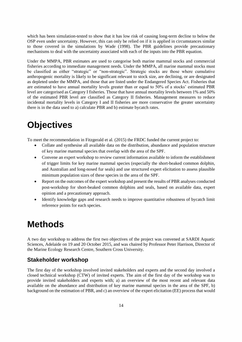
The current project reports on the outcomes of a workshop to synthesise available abundance data on key
marine mammal populations in the area of the SPF using expert judgement and the application or not of
PBR analyses using these data.
Expert elicitation
Expert elicitation (EE) has been used to obtain and synthesise expert opinion in situations where empirical
data are limited but a need exists to qualify or quantify risk (Martin et al. 2012, McBride et al. 2012). For
example, structured EE has been used to assess the IUCN Red list category of extinction risk for selected
Australian bird taxa (McBride et al. 2012), estimate abundance and trends of koala populations (Adams-
Hosking et al. 2016), seasonal relative abundance of adult right whales (Eublaena glacialis) in the mid-
Atlantic (Oedekoven et al. 2015) and estimate the effect of anthropogenic disturbance on harbour
porpoises (Phocoena phocoena) as inputs into a stochastic population model (King et al. 2015). In many
cases expert judgements are incorporated in Bayesian models where the elicited judgements are used as
model priors (see Martin et al. 2012 for review). Whilst the opinions elicited from these processes may
not always provide an adequate quantitative basis for subsequent actions, the degree of uncertainty and
sources of uncertainty in opinion can be recorded and assessed (Martin et al. 2012). These processes also
provide a means of identifying gaps in current knowledge and future data requirements for informing
management objectives.
Potential biological removal
Potential biological removal (PBR) is part of a formalised legal framework that uses a quantitative
approach to estimate limits to marine mammal bycatch in the United States (US) Marine Mammal
Protection Act 1972 (MMPA). The Act requires that all populations of marine mammal species (referred
to as “stocks”) are regularly assessed, and that bycatch is controlled to ensure that marine mammal stocks
do not fall below their optimum sustainable population level in waters under US jurisdiction. These
estimates of limits to anthropogenic mortality that a population can sustain before it is impacted are
calculated using PBR (Wade 1998). Anthropogenic impacts to a population can occur either via depletion
or prevention of recovery. Stock Assessment Reports (SARs) for each marine mammal population are
published annually by the US National Oceanic and Atmospheric Administration (NOAA) Fisheries. Each
SAR must include information on how the stock was defined, a minimum population estimate for that
stock, information on population trends and estimates of all anthropogenic mortality to the stock, as well
as estimates of anthropogenic mortality (NMFS 2016). The reports must also state whether cumulative
fisheries mortality to a stock is considered to be significant or insignificant. The level of significance is
determined relative to the Zero Mortality Rate Goal (ZMRG) which is a key goal of the MMPA. The
ZMRG states that “commercial fisheries shall reduce incidental mortality and serious injury of marine
mammals to insignificant levels approaching a zero mortality and serious injury rate”. Fisheries mortality
to a given stock is considered to be approaching ZMRG, if cumulative incidental fisheries mortality is less
than 10% of the calculated PBR for that stock (NMFS 2016). Conversely, if cumulative bycatch mortality
is estimated at greater than 10% of PBR calculated for a given stock, fisheries mortality to that stock is
not considered as being insignificant.
The PBR level is, conceptually, the maximum number of anthropogenic mortalities a marine mammal
population can sustain while still allowing that “stock” to reach or maintain its optimum sustainable
population (OSP). Under the MMPA a ‘stock’ (also referred to as a ‘population’ in this report) is defined
as ‘a group of marine mammals of the same species or smaller taxa in a common spatial arrangement that
interbreed when mature’. The OSP is defined as ‘the number of animals which will result in the maximum
productivity of the population or the species, keeping in mind the carrying capacity of the habitat and the
health of the ecosystem of which they form a constituent element.’ In practice, PBR levels have to be
calculated using inexact data, making a precautionary allowance for uncertainty. The PBR level is a long-
term average estimated limit of annual anthropogenic mortality. Wade (1998) proposed a simple formula,
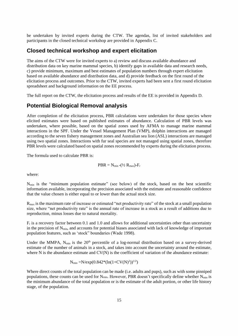
14
which has been simulation-tested to show that it has low risk of causing long-term decline to below the
OSP even under uncertainty. However, this can only be relied on if it is applied in circumstances similar
to those covered in the simulations by Wade (1998). The PBR guidelines provide precautionary
mechanisms to deal with the uncertainty associated with each of the inputs into the PBR equation.
Under the MMPA, PBR estimates are used to categorise both marine mammal stocks and commercial
fisheries according to immediate management needs. Under the MMPA, all marine mammal stocks must
be classified as either “strategic” or “non-strategic”. Strategic stocks are those where cumulative
anthropogenic mortality is likely to be significant relevant to stock size, are declining, or are designated
as depleted under the MMPA, and those that are listed under the Endangered Species Act. Fisheries that
are estimated to have annual mortality levels greater than or equal to 50% of a stocks’ estimated PBR
level are categorised as Category I fisheries. Those that have annual mortality levels between 1% and 50%
of the estimated PBR level are classified as Category II fisheries. Management measures to reduce
incidental mortality levels in Category I and II fisheries are more conservative the greater uncertainty
there is in the data used to a) calculate PBR and b) estimate bycatch rates.
Objectives
To meet the recommendation in Fitzgerald et al. (2015) the FRDC funded the current project to:
Collate and synthesise all available data on the distribution, abundance and population structure
of key marine mammal species that overlap with the area of the SPF.
Convene an expert workshop to review current information available to inform the establishment
of trigger limits for key marine mammal species (especially the short-beaked common dolphin,
and Australian and long-nosed fur seals) and use structured expert elicitation to assess plausible
minimum population sizes of these species in the area of the SPF.
Report on the outcomes of the expert workshop and present the results of PBR analyses conducted
post-workshop for short-beaked common dolphins and seals, based on available data, expert
opinion and a precautionary approach.
Identify knowledge gaps and research needs to improve quantitative robustness of bycatch limit
reference points for each species.
Methods
A two day workshop to address the first two objectives of the project was convened at SARDI Aquatic
Sciences, Adelaide on 19 and 20 October 2015, and was chaired by Professor Peter Harrison, Director of
the Marine Ecology Research Centre, Southern Cross University.
Stakeholder workshop
The first day of the workshop involved invited stakeholders and experts and the second day involved a
closed technical workshop (CTW) of invited experts. The aim of the first day of the workshop was to
provide invited stakeholders and experts with; a) an overview of the most recent and relevant data
available on the abundance and distribution of key marine mammal species in the area of the SPF, b)
background on the estimation of PBR, and c) an overview of the expert elicitation (EE) process that would
15
be undertaken by invited experts during the CTW. The agendas, list of invited stakeholders and
participants in the closed technical workshop are provided in Appendix C.
Closed technical workshop and expert elicitation
The aims of the CTW were for invited experts to a) review and discuss available abundance and
distribution data on key marine mammal species, b) identify gaps in available data and research needs,
c) provide minimum, maximum and best estimates of population numbers through expert elicitation
based on available abundance and distribution data, and d) provide feedback on the first round of the
elicitation process and outcomes. Prior to the CTW, invited experts had been sent a first round elicitation
spreadsheet and background information on the EE process.
The full report on the CTW, the elicitation process and results of the EE is provided in Appendix D.
Potential Biological Removal analysis
After completion of the elicitation process, PBR calculations were undertaken for those species where
elicited estimates were based on published estimates of abundance. Calculation of PBR levels was
undertaken, where possible, based on the spatial zones used by AFMA to manage marine mammal
interactions in the SPF. Under the Vessel Management Plan (VMP), dolphin interactions are managed
according to the seven fishery management zones and Australian sea lion (ASL) interactions are managed
using two spatial zones. Interactions with fur seal species are not managed using spatial zones, therefore
PBR levels were calculated based on spatial zones recommended by experts during the elicitation process.
The formula used to calculate PBR is:
PBR = Nmin *(½ Rmax)*Fr
where:
Nmin is the “minimum population estimate” (see below) of the stock, based on the best scientific
information available, incorporating the precision associated with the estimate and reasonable confidence
that the value chosen is either equal to or lower than the actual stock size.
Rmax is the maximum rate of increase or estimated “net productivity rate” of the stock at a small population
size, where “net productivity rate” is the annual rate of increase in a stock as a result of additions due to
reproduction, minus losses due to natural mortality.
Fr is a recovery factor between 0.1 and 1.0 and allows for additional uncertainties other than uncertainty
in the precision of Nmin, and accounts for potential biases associated with lack of knowledge of important
population features, such as ‘stock” boundaries (Wade 1998).
Under the MMPA, Nmin is the 20th percentile of a log-normal distribution based on a survey-derived
estimate of the number of animals in a stock, and takes into account the uncertainty around the estimate,
where N is the abundance estimate and CV(N) is the coefficient of variation of the abundance estimate:
Nmin =N/exp(0.842*(ln(1+CV(N)2))1/2)
Where direct counts of the total population can be made (i.e. adults and pups), such as with some pinniped
populations, these counts can be used for Nmin. However, PBR doesn’t specifically define whether Nmin is
the minimum abundance of the total population or is the estimate of the adult portion, or other life history
stage, of the population.

16
Default values of Rmax, the maximum rate of increase of a population, proposed by Wade (1998) are 0.04
for small cetaceans and 0.12 for pinnipeds. In the absence of information on specific maximum potential
growth rates for the populations considered in this report, these default values were used, in accordance
with proposed Guidelines for preparing SARs under the US MMPA (NMFS 2016). One source of
uncertainty in estimating Rmax is that as well as requiring data on the current population dynamics of a
“stock” it also assumes some knowledge of what that populations potential growth rate is, particularly
with respect to the effect of density dependence (e.g. recovery from depletion, resource competition).
The choice of recovery factor term, Fr, can allow for uncertainty in estimates of other parameters in the
PBR calculation, such as Rmax. Default values of Fr provided in the Guidelines for SARs under the MMPA
are 0.1 for endangered species (Listed under the US Endangered Species Act, 1973) and 0.5 for stocks
that are depleted and threatened or of unknown status (NMFS 2016) Values of 0.5-1.0 are used for stocks
that are known to be increasing (NMFS 2016). The selection of an appropriate recovery factor can be
improved if there is evidence that uncertainty is low around estimates of abundance or anthropogenic
mortality rates. This includes data detailing the age and / or sex of individuals that are being removed from
the population through anthropogenic mortality.
A number of assumptions are made in calculating PBR, the primary one is that Nmin is derived from a
single population. If the population structure of a species within the region that the PBR is being calculated
for is unknown and abundance estimates from a number of populations are pooled, the resulting PBR
levels will not meet this assumption. This is of particular concern if anthropogenic mortality is
disproportionate across different populations that have been pooled in the area (e.g. one population could
end up being adversely impacted even though aggregate PBR estimates related to bycatch rates suggest
otherwise).
Calculations of PBR were made after the completion of the CTW, with participants only providing input
into the Nmin used in these calculations. Full details of the CTW process, results and discussions are
provided in Appendix A. An 80% confidence interval was derived for Nmin based on the value of
confidence (integer between 50 and 100) assigned by each CTW participant to their individual estimate
ranges (Speirs-Bridge et al. 2010). Where no level of confidence was provided a default value of 80% was
assigned. The average minimum group EE estimates was then used as Nmin for PBR calculations. This is
very different to the US MMPA approach, where estimates are derived explicitly from abundance survey
data. In the absence of information on specific growth rates for the populations considered in this report,
we used default values of Rmax and FR used under the MMPA in accordance with proposed Guidelines for
Preparing Stock Assessment Reports (http://www.nmfs.noaa.gov/pr/sars/guidelines.htm) in the
calculations of PBR for the SPF.

17
Estimates of Nmin used in PBR calculations
Australian sea lions (ASL):
Estimates of Nmin for ASL were provided for each of the two ASL management zones used by AFMA
(Figure 1). These zones were considered appropriate by CTW participants based on the spatial distribution
of the WA and SA meta-populations.
Figure 1: The two management zones considered by participants during the second round of Expert
Elicitation when providing estimates of Australian sea lion abundance. These management zones reflect
those used by AFMA under the Australian sea lion management strategy.
Although ten CTW participants provided estimates of ASL abundance for each of the two AFMA
management zones, these elicited estimates were not used to calculate PBR. The mitochondrial DNA
structure of ASL indicate a high degree of natal philopatry, with extremely low rates of female
immigration and emigration between colonies (Campbell et al. 2008, Lowther et al. 2012). Consequently,
PBR was calculated at the individual colony/sub-population level. Therefore, estimates of Nmin for each
colony were derived from the most recent pup estimates for that colony to which a multiplier of 3.8 was
applied (Goldsworthy et al. 2015a). There are 71 known extant ASL breeding colonies within the area of
the SPF, with good recent abundance data for the colonies in Zone 2 (SA waters). Table 1 presents the
values used to calculate PBR for ASL at the individual colony/sub-population level.
18
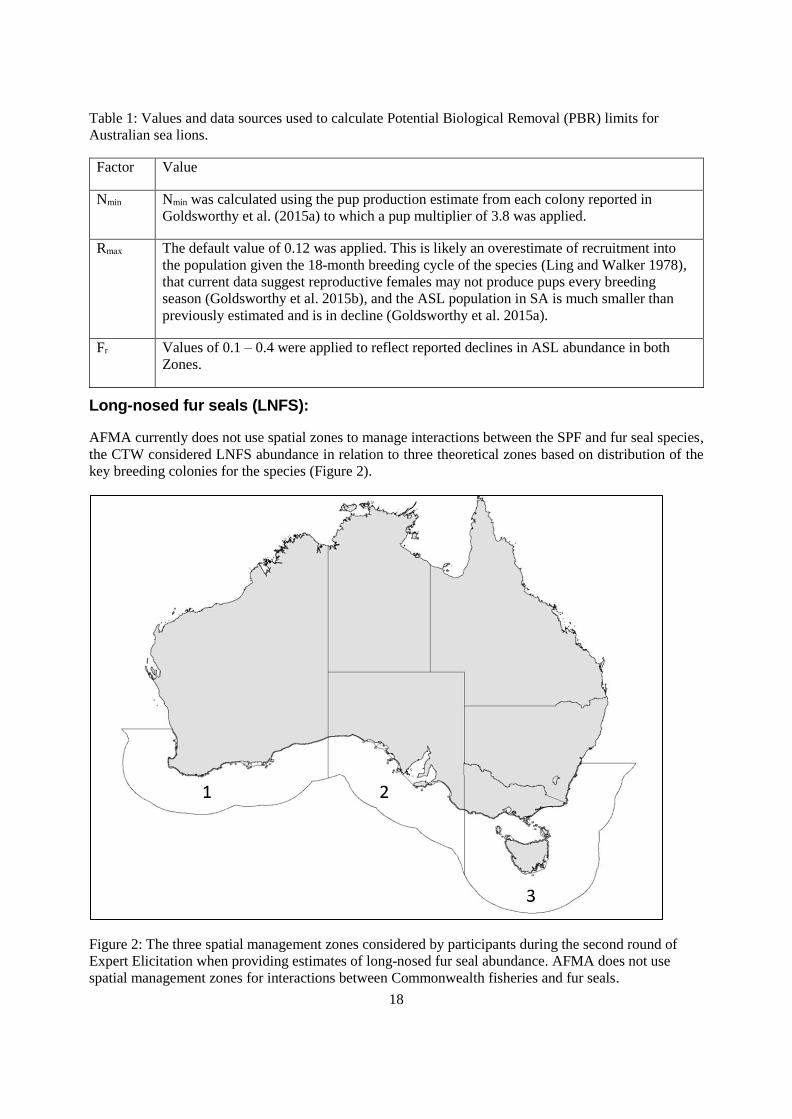
Table 1: Values and data sources used to calculate Potential Biological Removal (PBR) limits for
Australian sea lions.
Factor Value
Nmin Nmin was calculated using the pup production estimate from each colony reported in
Goldsworthy et al. (2015a) to which a pup multiplier of 3.8 was applied.
Rmax The default value of 0.12 was applied. This is likely an overestimate of recruitment into
the population given the 18-month breeding cycle of the species (Ling and Walker 1978),
that current data suggest reproductive females may not produce pups every breeding
season (Goldsworthy et al. 2015b), and the ASL population in SA is much smaller than
previously estimated and is in decline (Goldsworthy et al. 2015a).
Fr Values of 0.1 – 0.4 were applied to reflect reported declines in ASL abundance in both
Zones.
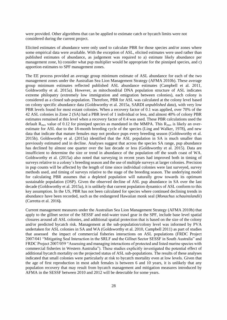
Long-nosed fur seals (LNFS):
AFMA currently does not use spatial zones to manage interactions between the SPF and fur seal species,
the CTW considered LNFS abundance in relation to three theoretical zones based on distribution of the
key breeding colonies for the species (Figure 2).
Figure 2: The three spatial management zones considered by participants during the second round of
Expert Elicitation when providing estimates of long-nosed fur seal abundance. AFMA does not use
spatial management zones for interactions between Commonwealth fisheries and fur seals.

19
Eleven participants provided estimates of LNFS abundance in the three proposed spatial zones. After
estimates were adjusted relative to the level of confidence expressed with each individual response, the
average lowest EE estimate of LNFS abundance was 14,379 (S.E. 1,287) for Zone 1, 83,292 (S.E. 7,685)
for Zone 2 and 2,708 (S.E. 363) for Zone 3. Table 2 presents the values used to calculate PBR for LNFS
for each of the three Zones.
Table 2: Values and data sources used to calculate Potential Biological Removal (PBR) limits for long-
nosed fur seals.
Factor Value
Nmin The Nmin values used were the lowest average estimate from eleven respondents to the
Expert Elicitation process for each management zone. Zone 1 = 14,379; Zone 2 = 83,292;
Zone 3 = 2,708.
Rmax The population growth rate of LNFS in WA (Zone 1) was calculated to be 1.1% per
annum between 1999 and 2011 (Campbell et al. 2014), although estimated population
growth varied between colonies, ranging from -6.6% to + 6.7% annually. A state-wide
survey conducted across SA in the 2013-14 breeding season (Zone 2) estimated pup
production to be 3.6 times greater than the 1989-90 estimate (Shaughnessy et al. 2015).
The combined pup production estimates for Victoria, the Tasmanian Bass Strait colonies
and NSW (Zone 3) were found to have increased by 8% between 2008 and 2014
(McIntosh et al. 2014). Although data exists on abundance trends for some pinniped
species in the USA, we could not find an example of PBR where a value other than the
default R max of 0.12 was used. Therefore the default value of 0.12 was used for PBR
calculations in the current study.
Fr A range of recovery factors from 0.5 to 0.9 were used to reflect potential stable to
increasing population growth rates in all zones. Recovery factors of 1.0 are reserved for
cases where there is assurance that estimates of Nmin, Rmax and estimates of anthropogenic
mortality are unbiased (NMFS 2016).
Australian fur seals (AUFS):
As AFMA does not use spatial zones to manage interactions with fur seals, the CTW considered AUFS
abundance in relation to a single theoretical management zone based on the distribution of breeding
colonies and known ecology of the species (Figure 3).
After estimates were adjusted relative to the level of confidence expressed with each individual response,
the average lowest estimate of AUFS abundance from eleven responses was 87,424 (S.E. 10,415). Table
3 presents the values used to calculate PBR for AUFS for a single management zone.

20
Figure 3: The single management zone considered by participants during the second round of Expert
Elicitation when providing estimates of Australian fur seal abundance. AFMA does not use spatial
management zones for interactions between Commonwealth fisheries and fur seals.
Table 3: Values and data sources used to calculate Potential Biological Removal (PBR) limits for
Australian fur seals.
Factor Value
Nmin The Nmin values used were the lowest average estimate from eleven respondents to Expert
Elicitation process for the single management zone. Zone 1 = 87,424.
Rmax Average annual increases in pup production growth rates have been observed between1986-
87 and 2002-03 (5%) and between 2002-03 and 2007-08 (0.3%), with a decrease observed
between 2007-08 and 2013-14 (6%). Although new sites have been colonised at the edges of
the range of AUFS, trends in abundance are unclear. Due to this uncertainty, the default
Rmax used under the MMPA (0.12) was used.
Fr A range of recovery factors from 0.5 to 0.9 were used to reflect potential stable to increasing
population growth rates in all zones. Recovery factors of 1.0 are reserved for cases where
there is assurance that estimates of Nmin, Rmax and estimates of anthropogenic mortality are
unbiased (NMFS 2016).

21
Short beaked common dolphins (SBCD):
Most CTW participants did not think it was appropriate to provide estimates for SBCD abundance for
those zones where there were no empirical abundance data available. Published abundance estimates for
SBCDs only exist for a discrete area that partially overlaps with SPF management Zone 3 (Bilgmann et
al. 2014a). Estimates of Nmin for SBCD were provided by a total of six participants for Zone 3 (Figure 4).
Two experts stated that the reason they did not provide estimates was that they did not agree with PBR
estimation for this species in relation to SPF management zones, as the zones do not reflect published data
on population structuring for SBCD across this area (Möller et al. 2011, Bilgmann et al. 2014b). This
included the identification of two genetic populations co-occurring in Zone 3 (Bilgmann et al. 2014b).
Figure 4: The seven management zones considered by participants during the second round of Expert
Elicitation when providing estimates of short-beaked common dolphin abundance. These seven
management zones are used by AFMA to manage dolphin interactions within the SPF.
After estimates were adjusted relative to the level of confidence expressed with each individual’s response,
the average lowest estimate from for SBCD abundance in Zone 3 was 26,117. Table 4 presents the values
used to calculate PBR for SBCD Management Zone 3.

22
Table 4: Values and data sources used to calculate Potential Biological Removal (PBR) limits for short
beaked common dolphin in Management Zone 3.
Factor Value
Nmin The Nmin value used was the lowest average estimate from six respondents to Expert
Elicitation process. Zone 3 = 26,117.
Rmax The maximum growth rate for SBCD is not well understood anywhere across its range in
Australian waters. An Rmax of 0.04 was used following the default value for small
cetaceans under the MMPA.
Fr In accordance with NFMS (2016) an FR value of 0.5 was used as the default status for a
stock that is considered of unknown status.
Tursiops spp.:
No estimates of abundance were made for offshore common bottlenose dolphins during the EE, as there
are no data on the abundance, offshore density, population structure or distribution of this species in the
area of the SPF.
The common bottlenose dolphin can occur sympatrically with the Indo-Pacific bottlenose dolphin, and
assessment of abundance of inshore bottlenose dolphins in the southern Australian region is further
complicated by the unresolved taxonomy of the Tursiops genus, with two species described from inshore
waters, the Indo-Pacific bottlenose dolphin T. aduncus and the Burrunan dolphin, T. australis (Charlton-
Robb et al. 2011). The Indo-Pacific bottlenose dolphin has an extensive distribution in shelf waters of
Australia, and while a number of abundance estimates exist for this species, these tend to be for small
restricted areas where dolphins exhibit some degree of residency (see Woinarski et al. 2014). Therefore,
there remains no abundance data for this species for much of its coastal range. Between four and six CTW
participants provided estimates of abundance for inshore bottlenose dolphins in the area of the seven
bycatch management zones, and additional geographically specified areas within the management zones
that were agreed by the CTW participants. Zone 3a represents the SA Gulfs and Investigator Strait, Zone
4a represents Port Philip Bay and Western Port, Victoria, 6a represents the Gippsland Lakes, Victoria.
After estimates were adjusted relative to the level of confidence expressed with each individual’s response,
the average lowest estimate ranged from a few tens to less than 200 individuals.
Given that the abundance and population structure of inshore bottlenose dolphin species across the range
of the SPF is unknown we calculated PBR for resident populations where there are published abundance
estimates using the default values of Rmax (0.04) and Fr (0.5).

23
Results
PBR Analysis
PBR Analysis – Australian sea lion
PBR estimates for each ASL colony in each of the two management zones for a range of recovery values
are presented in Table 5a and 5b. Using a recovery factor of 0.1, individual colony PBR ranged from 0-1
individuals in Zone 1 and 0-11 individuals in Zone 2. Using a recovery factor of 0.4, individual colony
PBR ranged from 0-5 individuals in Zone 1, and 0-44 individuals in Zone 2. The use of the default value
of 0.12 is most likely an overestimate of Rmax for ASL as the most recent comprehensive abundance data
for the species in SA shows a decline of approximately 23% at 32 breeding sites which had been surveyed
6-11 years earlier (Goldsworthy et al. 2015a).
Table 5a. Potential Biological Removal (PBR) values for cumulative annual anthropogenic mortalities of
Australian sea lions (ALS) in Zone 1 of the SPF management area. Nmin was calculated using the most
recent pup estimates for that colony and a pup multiplier of 3.8. Sources of pup estimates are Dennis and
Shaughnessy 19961, Gales et al. 19942 and the Department of Parks and Wildlife, Western Australia3. Rmax
is the maximum growth rate, FR is the recovery factor (range 0.1-0.4).
Breeding site Abundance
estimate
Rmax Range of PBRs based on Fr values; 0.1 -0.4
to 0.4 0.1 0.2 0.3 0.4
Twilight Cove1 15 0.12 0 0 0 0
Spindle Is. 3 201 0.12 1 2 4 5
Ford (Halfway) Is.3 91 0.12 1 1 2 2
Round Is.2 49 0.12 0 1 1 1
Salisbury Is. 2 38 0.12 0 0 1 1
Wickham (Stanley ) Is. 3 68 0.12 0 1 1 2
Glennie Is. 3 80 0.12 0 1 1 2
Taylor Is. 3 15 0.12 0 0 0 0
Kimberley Is. 3 122 0.12 1 1 2 3
MacKenzie Is. 3 19 0.12 0 0 0 0
Rocky (Investigator) Is. 3 61 0.12 0 1 1 1
West Is. 3 76 0.12 0 1 1 2
Red Islet3 103 0.12 1 1 2 2
Middle Doubtful Is. 3 38 0.12 0 0 1 1
Hauloff Rock3 84 0.12 1 1 2 2
Kermadec (Wedge) Is. 3 15 0.12 0 0 0 0
Poison Creek Is. 3 8 0.12 0 0 0 0
Little Is. 3 4 0.12 0 0 0 0
Cooper Is. 30 0.12 0 0 1 1
Twin Peaks. 3 4 0.12 0 0 0 0
Six Mile Is. 3 152 0.12 1 2 3 4

24
Table 5b. Potential Biological Removal (PBR) values for cumulative annual anthropogenic mortalities
of Australian sea lions (ASL) in Zone 2 in the SPF management area. Nmin was calculated using colony
pup production estimates in Goldsworthy et al. (2015a) and a pup multiplier of 3.8. Rmax is the maximum
growth rate, FR is the recovery factor (range 0.1-0.4).
Breeding site Abundance estimate Rmax Range of PBRs for Fr values; 0.1 to 0.4
0.1 0.2 0.3 0.4
The Pages Islands 1816 0.12 11 22 33 44
Seal Slide (Kangaroo Is.) 30 0.12 0 0 1 1
Black Point (Kangaroo Is.) 4 0.12 0 0 0 0
Seal Bay (Kangaroo Is.) 984 0.12 6 12 18 24
Cape Bouguer (Kangaroo Is.) 34 0.12 0 0 1 1
North Casuarina Is. (Kangaroo Is.) 42 0.12 0 1 1 1
Peaked Rocks 220 0.12 1 3 4 5
North Islet 80 0.12 0 1 1 2
Dangerous Reef 1843 0.12 11 22 33 44
English Is. 129 0.12 1 2 2 3
Albatross Is. 262 0.12 2 3 5 6
South Neptune Islands 27 0.12 0 0 0 1
North Neptune Islands 34 0.12 0 0 1 1
Lewis Is. 312 0.12 2 4 6 7
Williams Is. 19 0.12 0 0 0 0
Curta Rocks 27 0.12 0 0 0 1
Liguanea Is. 95 0.12 1 1 2 2
Price Is. 122 0.12 1 1 2 3
Little Hummock Is. 15 0.12 0 0 0 0
Four Hummocks Is. 23 0.12 0 0 0 1
Rocky (South) Is. 42 0.12 0 1 1 1
Rocky (North) Is. 133 0.12 1 2 2 3
Cap Island 118 0.12 1 1 2 3
West Waldegrave Is. 338 0.12 2 4 6 8
Jones Is. 72 0.12 0 1 1 2
Point Labatt 8 0.12 0 0 0 0
Pearson Is. 114 0.12 1 1 2 3
Ward Is. 167 0.12 1 2 3 4
Nicolas Baudin Is. 239 0.12 1 3 4 6
Olive Is. 505 0.12 3 6 9 12
Lilliput 274 0.12 2 3 5 7
Blefuscu 369 0.12 2 4 7 9
Breakwater Is. 103 0.12 1 1 2 2
Lounds Is. 76 0.12 0 1 1 2
Fenelon Is. 72 0.12 0 1 1 2
West Is. 76 0.12 0 1 1 2
Purdie Is. 255 0.12 2 3 5 6
Nuyts Reef (x3) 399 0.12 2 5 7 10
Bunda 02 (B1.1) 11 0.12 0 0 0 0
Bunda 06 (B3) 34 0.12 0 0 1 1
Bunda 19 (B8) 27 0.12 0 0 0 1

25
PBR Analysis – Long-nosed fur seal
PBR estimates for LNFS in each of the three proposed management zones for a range of recovery values
are presented in Table 6.
Table 6. Potential Biological Removal (PBR) values for cumulative annual anthropogenic mortalities of
long-nosed fur seals (LNFS) in three proposed zones in the SPF management area. Nmin from expert
elicitation represent the group average lowest plausible and group average best estimates of abundance.
Rmax is the maximum growth rate, FR is the recovery factor (range 0.5-1).
LNFS
Zone
Nmin:
average
lowest
estimate
from 11
respondents
Rmax Range of PBRs based on Fr values:0.5 to 0.9
0.5 0.6 0.7 0.8 0.9
1 14,379 0.12 431 518 604 690 776
2 83,292 0.12 2,499 2,999 3,498 3,998 4,498
3 2,708 0.12 81 97 114 130 146
PBR Analysis – Australian fur seal
PBR estimates for AUFS within the proposed single management zone were calculated using a range of
recovery values and are presented in Table 7.
Table 7. Potential Biological Removal (PBR) values for cumulative annual anthropogenic mortalities of
Australian fur seals (AUFS) in in the SPF management area. Nmin is the minimum abundance estimate,
Rmax is the maximum growth rate, Fr is the recovery factor.
AUFS
Zone
Nmin: average
lowest
estimate from
11
respondents
Rmax Range of PBRs based on Fr values:0.5 to 0.9
0.5 0.6 0.7 0.8 0.9
1 87,424 0.12 2,623 3,147 3,672 4,196 4,721

26
PBR Analysis – short-beaked common dolphin in Zone 3
PBR estimates for SBCD were only conducted on EE estimates provided for management Zone 3 (Table
8).
Table 8. Potential Biological Removal (PBR) values for cumulative annual anthropogenic mortalities of
short beaked common dolphins (SBCD) considering abundance estimates from state waters of the Gulfs
and / or on shelf-waters <100m depth within Zone 3 of the SPF bycatch management area.
SBCD
Zone
Nmin: average lowest estimate
from 6 respondents
Rmax PBR value based on Fr value of
0.5
3 26,117 0.04 261
PBR Analysis – example for inshore bottlenose dolphin species
Example PBR estimates for bottlenose dolphin were calculated using a recovery factor of 0.5 and the
default maximum growth rate for cetaceans of 0.04. Published abundance estimates for resident
populations in the area of the SPF were used as Nmin.
Table 9. Potential Biological Removal (PBR) values for cumulative annual anthropogenic mortalities for
populations of coastal bottlenose dolphins (Tursiops species) based on published estimates of
abundance.
Resident coastal bottlenose dolphin
population size
Rmax PBR value based on Fr value of
0.5
63 (Bunbury, WA. Smith et al. 2013) 0.04 0.6
80 (Port Philip Bay, Vic. Reviewed in
Woinarski et al. 2014
0.04 0.8
63 (Jervis Bay, NSW. Möller et al. 2002) 0.04 0.6
143 (Port Stephens, NSW. Möller et al.
2002)
0.04 1.4
860 (Ballina coastal region, NSW. Reviewed
in Woinarski et al. 2014)
0.04 8.6

27
Discussion
Closed technical workshop (CTW)
The key objective of the CTW was to “review current information available to inform the establishment
of trigger limits using PBR for key marine mammal species (especially the short-beaked common dolphin,
and Australian and long-nosed fur seals)”. The CTW was successful in providing a synthesis of the current
information available on the abundance, distribution and ecology of Australian sea lions (ASL), Australian
fur seals (AUFS), long-nosed fur seals (LNFS), short-beaked common dolphins (SBCD) and inshore
bottlenose dolphins. Workshop discussions focused on factors affecting the precision of abundance
estimates and highlighted data gaps for each species (see Appendix A for full discussion).
The key concern raised by participants in the CTW was that while EE can provide a means of synthesising
expert judgment, it should not be used as a process to obtain qualitative “estimates” of abundance where
those estimates are then used to calculate trigger limits or thresholds for anthropogenic mortality using
PBR. As a result, two participants of the CTW declined to participate in the elicitation process. A further
three attendees did not provide estimates for any species or zones. Of those participants who did provide
estimates, the total number of respondents reflected the amount of available abundance data by species
and SPF management zones. Eleven participants provided estimates for the two fur seal species and ten
for ASL. Six participants provided estimates for SBCD for the one zone where abundance estimates are
available, while four to six (dependent on zone) provided estimates for inshore bottlenose dolphins.
Participants agreed that as there were no data available on abundance of offshore bottlenose dolphins,
estimates could not be given for this species.
Several participants noted that there are well-established procedures for estimating marine mammal
abundance (e.g. using line-transect, count, and/or mark-recapture surveys), which could be applied to the
species/areas of interest considered during the CTW. A number of participants stressed that estimates of
abundance collected using established methods were required to inform management action, particularly
with respect to calculating trigger limits, and that expert opinion should not be used to provide estimates
where no empirical data were available. As noted by Morgan (2014) “Rather, expert elicitation should
build on and use the best available research and analysis and be undertaken only when, given those, the
state of knowledge will remain insufficient to support timely informed assessment and decision making”
In general, estimates provided through the EE process reflected published abundance estimates where
such information was available. For species and zones where there were no available abundance data,
fewer participants provided estimates, and there was high variability in the lowest plausible estimates of
abundance provided. Sutherland and Burgman (2015) emphasised that the quality of the data obtained
through EE needs to be considered before such data are used to inform decision-making or in subsequent
analysis. The wide ranges in minimum and maximum estimates provided for some species and areas
during the CTW indicate that in the absence of actual abundance data, there was no consensus between
participants on what likely abundance estimates may be. Wide confidence intervals around estimates of
some species/zones showed that even with abundance data available, there was variation in how total
estimates were apportioned to management zones.
PBR analyses
The undertaking of PBR analyses was a component of this project as a result of a recommendation of a
previous FRDC workshop (Fitzgerald et al. 2015) where PBR was identified as a possible means of
estimating sustainable limits to anthropogenic mortality of marine mammal species interacting with the
SPF. Calculation of PBR levels was undertaken by the authors after results of the second round of EE
28
were provided. Other algorithms that can be applied to estimate catch or bycatch limits were not
considered during the current project.
Elicited estimates of abundance were only used to calculate PBR for those species and/or zones where
some empirical data were available. With the exception of ASL, elicited estimates were used rather than
published estimates of abundance, as judgement was required to a) estimate likely abundance per
management zone, b) consider what pup multiplier would be appropriate for the pinniped species, and c)
apportion estimates to SPF management zones.
The EE process provided an average group minimum estimate of ASL abundance for each of the two
management zones under the Australian Sea Lion Management Strategy (AFMA 2010b). These average
group minimum estimates reflected published ASL abundance estimates (Campbell et al. 2011,
Goldsworthy et al. 2015a). However, as mitochondrial DNA population structure of ASL indicates
extreme philopatry (extremely low immigration and emigration between colonies), each colony is
considered as a closed sub-population. Therefore, PBR for ASL was calculated at the colony level based
on colony specific abundance data (Goldsworthy et al. 2015a, SARDI unpublished data), with very low
PBR levels found for most extant colonies. When a recovery factor of 0.1 was applied, over 70% of the
42 ASL colonies in Zone 2 (SA) had a PBR level of 1 individual or less, and almost 40% of colony PBR
estimates remained at this level when a recovery factor of 0.4 was used. These PBR calculations used the
default Rmax value of 0.12 for pinniped species as mandated in the MMPA. This Rmax is likely an over-
estimate for ASL due to the 18-month breeding cycle of the species (Ling and Walker, 1978), and new
data that indicate that mature females may not produce pups every breeding season (Goldsworthy et al.
2015b). Goldsworthy et al. (2015a) identified that the ASL population in SA is much smaller than
previously estimated and in decline. Analyses suggest that across the species SA range, pup abundance
has declined by almost one quarter over the last decade or less (Goldsworthy et al. 2015). Data are
insufficient to determine the size or trend in abundance of the population off the south coast of WA.
Goldsworthy et al. (2015a) also noted that surveying in recent years had improved both in timing of
surveys relative to a colony’s breeding season and the use of multiple surveys at larger colonies. Precision
in pup counts will be affected by the length of time since individual colonies were last surveyed, survey
methods used, and timing of surveys relative to the stage of the breeding season. The underlying model
for calculating PBR assumes that a depleted population will naturally grow towards its optimum
sustainable population (OSP). Given the observed decline of ASL pup abundance in SA over the last
decade (Goldsworthy et al. 2015a), it is unlikely that current population dynamics of ASL conform to this
key assumption. In the US, PBR has not been calculated for species where continued declining trends in
abundance have been recorded, such as the endangered Hawaiian monk seal (Monachus schauinslandii)
(Carretta et al. 2016).
Current management measures under the Australian Sea Lion Management Strategy (AFMA 2010b) that
apply to the gillnet sector of the SESSF and mid-water trawl gear in the SPF, include base level spatial
closures around all ASL colonies, and additional spatial protection that is based on the size of the colony
and/or predicted bycatch risk. Management at the sub-population/colony level was informed by PVA
undertaken for ASL colonies in SA and WA (Goldsworthy et al. 2010, Campbell 2011) as part of studies
that assessed the impact of commercial fisheries interactions on ASL populations (FRDC Project
2007/041 “Mitigating Seal Interaction in the SRLF and the Gillnet Sector SESSF in South Australia” and
FRDC Project 2007/059 “Assessing and managing interactions of protected and listed marine species with
commercial fisheries in Western Australia”). These studies explicitly investigated the potential effect of
additional bycatch mortality on the projected status of ASL sub-populations. The results of these analyses
indicated that small colonies were particularly at risk to bycatch mortality even at low levels. Given that
the age of first reproduction in most adult females is between 6 and 10 years, it is unlikely that any
population recovery that may result from bycatch management and mitigation measures introduced by
AFMA in the SESSF between 2010 and 2012 will be detectable for some years.

29
Levels of PBR for LNFS were calculated for three potential spatial management zones that experts agreed
best reflected their distribution. A range of recovery factors from 0.5-0.9 were used to reflect that the
abundance of the species is increasing, although at different rates across its range in Australia (Campbell
et al. 2011, McIntosh et al. 2014, Shaughnessy et al. 2015). Estimates of PBR limits ranged from 431-776
for Zone 1, 2,499-4,498 for Zone 2 and 81-146 for Zone 3. The three spatial zones considered for LNFS
during the EE were based on the fact that the majority of breeding colonies for the species in Australia
occur in SA (Shaughnessy et al. 2015). Therefore, they do not consider the at sea distribution of this
species. Satellite tracking studies have shown variation in foraging strategies between different age and
sex classes. Adult females nursing pups will initially forage in mid-outer shelf waters before shifting to
much longer foraging trips to pelagic waters associated with the Subtropical Front (Baylis et al. 2012),
while adult and sub-adult males forage along the continental shelf (Page et al. 2006, SARDI unpublished
data). Movement of LNFS have been recorded between haul-outs in SA to Tasmania and New South
Wales, and longer range movement between New Zealand and NSW has also been recorded (Shaughnessy
et al. 2001, SARDI unpublished data). In the US, recent PBRs calculated for northern fur seal (Callorhinus
ursinus) were 451 for the California stock that has an abundance estimate of 14,050 (Carretta et al. 2016),
and 11,802 for the Eastern Pacific stock that has an abundance estimate of 648,534 (Munto et al. 2015).
LNFS were identified as a medium risk species from midwater trawling under the Level 2 PSA Residual
Risk Analysis under the ERAERF (AFMA 2010a). Bycatch of LNFS has been reported in AFMA
logbooks in both the gillnet and South East Trawl (SET) sectors of the SESSF, although bycaught seals
are not always identified to species. Under the US MMPA stock assessment guidance, cumulative fisheries
mortality is considered insignificant and approaching a zero mortality if it is less than 10% of calculated
PBR (NMFS 2016). Therefore, while PBR provides a calculated reference limit for cumulative
anthropogenic mortality, the goal of the MMPA is to ensure such mortalities are insignificant and
approaching zero. For LNFS, 10% of the calculated PBR is 43-69 individuals for Zone 1, 250-400 for
Zone 2, and 8-13 for Zone 3. The continued recovery of LNFS abundance and impacts of this recovery in
terms of future interactions with fisheries, both ecological and operational, was raised on the first day of
the stakeholder workshop. Modelling potential ecological interactions under different future population
scenarios can inform adaptive management of seal-fishery interactions.
A PBR level was calculated for AUFS based on a single spatial management zone that experts agreed best
reflected the distribution and consideration of the species as a single panmictic population (Lancaster et
al. 2010). As with LNFS, a range of recovery factors from 0.5-0.9 were used to reflect a general increasing
trend in abundance as well as range expansion/recolonisation of AUFS (Kirkwood et al. 2005, 2010,
McIntosh et al. 2014). Estimates of cumulative anthropogenic PBR levels ranged from 2,623-4,721
individuals. Ten percent of this PBR level would range between 262 and 420 individuals. Fisheries
interactions have been identified as the most significant and threatening processes for this species. A
review of bycatch levels of AUFS in the SET sector of the SESSF estimated an annual bycatch of 597 fur
seals in the ‘wet boat’ sector of the fishery, based on observed bycatch mortality rates between 1993 and
2010 (Expert Panel on a Declared Commercial Fishing Activity 2014). While the PBR limits we estimated
are higher than the bycatch number reported in the SET, bycatch levels may be above 10% of the
calculated PBR and, following the guidelines for preparing stock assessment reports under the MMPA
(NMFS 2016), would therefore be considered as significant and not approaching the ZMRG.
Calculating PBR for a population assumes that anthropogenic mortality impacts age and sex classes
equally. The sex composition of fur seals caught in the SET has only been assessed in the winter blue
grenadier trawl fishery component off western Tasmania, where bycatch appears to be strongly male
biased (94% of examined AUFS bycaught over three seasons, Tilzey et al. 2006, FRDC Project No.
2001/008). Tracking studies have shown that this is a region where male fur seals predominantly forage
(Tilzey et al. 2006, Arnould and Kirkwood 2008, Kirkwood and Arnould 2011). The sex ratio of bycaught
fur seals has not been assessed in other regions of the fishery that overlap more with the core female
foraging regions in eastern and western Bass Strait (Arnould and Kirkwood 2008, Kirkwood and Arnould

30
2011). Female AUFS typically show strong fidelity to foraging hotspots and have varying lengths of
foraging trips dependent on the distance of the colony from the shelf edge (Arnould and Kirkwood 2008,
Kirkwood and Arnould 2011), and are at greater risk of interacting with mid-water trawl gear where
foraging and fishing areas overlap. If bycatch mortality disproportionately affects breeding females in
some areas of their foraging range, this higher removal rate would need to be factored into PBR
calculations which could be achieved by adjusting the recovery factor, or rate of population increase if
this was known. The amount of certainty in levels of anthropogenic removal can also guide management
decisions on the value of recovery factor used. If there is high precision in estimates of cumulative
anthropogenic mortality then the recovery factor could be increased.
The CTW participants considered SBCD abundance in relation to the seven management zones currently
used by AFMA to manage interactions with dolphins in the SPF. The group noted that the current spatial
delineation of the seven SPF management zones does not reflect recently published analyses of population
structure of SBCD in Australian waters (Möller et al. 2011, Bilgmann et al. 2014b). Two participants
withdrew from providing estimates for SBCD as they did not agree with either the EE process for this
species or the delineation of the seven zones used by AFMA to manage dolphin interactions. Published
abundance data are only available for a small region of Zone 3, therefore a PBR level was only calculated
using lowest average EE estimates provided by six participants for this Zone. The CTW noted that
published abundance estimates for SBCD are restricted to the SA Gulfs and waters less than 100 m in
depth in Zone 3 (Filby et al. 2010, Möller et al. 2012) or to waters out to 100 m off the Eyre Peninsula
(Bilgmann et al. 2014a). There are no data on the abundance of SBCD in off-shelf waters in Zone 3, or
elsewhere across their range. The level of mixing of individuals, either spatially or genetically, between
inshore and offshore areas is unknown, and there are no data on trends in abundance for this species in
Australian waters.
Using a recovery factor of 0.5, the default value for stocks of unknown status (NMFS 2016), and an
elicited estimate of abundance, the calculated PBR limit for Zone 3 was 261 individuals Therefore, the
level where cumulative annual fishing mortality would be considered insignificant and approaching
ZMRG (10% of PBR) for this Zone was 26 individuals. Within the area of SA where abundance data are
available, SBCD bycatch is currently reported in the gillnet sector of the SESSF and purse-seine fishing
operations of the State managed South Australian Sardine Fishery (SASF) (Ward et al. 2015). Interactions
with the gillnet sector of the SESSF are managed under the Dolphin Strategy to minimise bycatch through
performance criteria set at an individual boat level based on trigger limits and assessed through Electronic
Monitoring (EM) and logbook reporting (AFMA 2014b). These individual vessel based management
measures are currently only implemented in the Coorong Zone of the fishery, but are intended to be
implemented in conjunction with EM across all zones where gillnet operations occur. A total of 78 dolphin
mortalities have been reported in protected species interaction reports from Commonwealth gillnet
operations between March 2012 and March 2016. Dolphin interactions with the SASF are managed
through an industry Code of Practice (CoP) and effectiveness of the CoP is assessed by the SA Department
of Primary Industries and Regions (PIRSA) Fisheries and Aquaculture who manage the fishery using data
collected by onboard observers.
During the CTW, the recorded co-occurrence of SBCD from two different genetic populations within
Management Zone 3 of the SPF, and data indicating longitudinal movement of individuals from different
populations between SPF management zones (Bilgmann et al. 2014b), was discussed. Two participants
stated that the identification of two populations in Zone 3 rendered PBR inappropriate for this Zone. Other
participants considered these data but felt that there was still considerable uncertainty in the extent of
population sub-structuring in SBCD, and the level that it is relevant to their management (i.e. in the PBR
context do the Management Units proposed by Bilgmann et al. 2014b equate to a “stock”). Comments
from CTW participants indicated that estimates provided for Zone 3 were based on published aerial survey
data (Möller et al. 2012, Bilgmann et al. 2014a). The elicited estimate of Nmin used to calculate PBR is
within the confidence intervals of the aerial survey abundance estimates of SBCD for the eastern Great

31
Australian Bight, between Ceduna and Coffin Bay and out to the 100 m depth contour (Bilgmann et al.
2014a) which is only a portion of the total area of management Zone 3.
Möller et al. (2012) reported on a preliminary PBR analysis based on the abundance estimates generated
from a winter and summer aerial survey conducted in the South Australian Gulfs and waters out to the
100 m depth contour. They used a recovery factor of 0.5 and an R max of both 0.04 and 0.02 in their
calculations (Möller et al. 2012). PBR from summer abundance estimates were calculated as 61 and 122
for Rmax values of 0.2 and 0.4, respectively. PBR from winter abundance estimates was calculated as 92
and 183 for Rmax values of 0.2 and 0.4, respectively. Möller et al. (2012) state that ‘analyses and subsequent
interpretations of SBCD abundance estimates and PBR calculations presented in the report are preliminary
and highly simplified for expediency. The estimates provided are not definitive and should not be used
for informing any management decisions at this stage’. Möller et a.l (2012) chose the lower value of Rmax
to account for potential lower reproductive rate that may be caused by cryptic mortality (i.e. unseen
mortality) such as separation of calves from mothers (Archer et al. 2004), that may not be recorded during
observed interactions with the SASF. In the Eastern Tropical Pacific (ETP), interactions between dolphins
(predominantly spotted Stenella attenuata and spinner dolphins S. longirostris) and commercial purse
seine operations for tuna have occurred since the late 1950s, resulting in high mortality rates until the
1980s when increased regulations, observer programs and changes to fishing gear and practices led to a
significant reduction in mortalities (Hall 1998). However, the recovery of these species since bycatch has
been reduced has been slower than is expected for small cetaceans (Gerrodette and Forcada 2005, Wade
et al. 2007). The suggested reasons for a lack of observed recovery, that are not necessarily independent,
include under-estimation of bycatch rates including cryptic mortality, potential negative effects on
reproduction and survival that continued chase and encirclement of dolphins may have through elevated
stress or increased energetic demands, and potential effects of ecosystem changes in the ETP (Gerrodette
and Forcada 2005, Wade et al. 2007). In contrast to the ETP tuna purse seine fishery, dolphin interactions
with the SASF do not involve chases.
Fine-scale population sub-structuring of SBCD has been reported in Australian waters (Bilgmann et al
2014b) and in the Pacific US and coast of New Zealand (Amaral et al. 2012). This is in contrast to levels
of structuring reported for SBCD in the Atlantic. In the Northwest Atlantic, SBCD are considered a single
panmictic population with a recent abundance estimate of 173,486 (CV=0.55) (Waring et al. 2015). The
estimate was derived from an aerial survey of the Atlantic Canadian coast from North Labrador to the
Scotian Shelf after correcting for perception and availability bias (Lawson and Gosselin 2009). Shipboard
surveys were also conducted between the lower Bay of Fundy and North Carolina in 2011, and led to
estimated SBCD abundance of 54,507 (CV=0.30) in shelf waters between the 100 and 200 m depth
contours, and 9,828 (CV=0.71) in waters between 200 m and offshore of the 2000 m depth contour (Palka
2012). The current PBR for the stock based on an Rmax of 0.04 and a Fr of 0.5 is 1,125 (Waring et al. 2015).
The average annual mortality rate of SBCD combined for US fisheries in the Northwest Atlantic between
2009 and 2013 was estimated at 363 individuals, so was greater than 10% of PBR (Waring et al. 2015).
SBCD bycatch was observed in gillnet, mid-water and bottom trawl and pelagic long line gear (Waring et
al. 2015). In the Northeast Atlantic, SBCD ranging from waters off Scotland to Portugal are considered a
single panmictic population (ICES 2013, Moura et al. 2013), and on the European Atlantic shelf
population size is estimated at 56,221 (CV=0.234) (Hammond et al. 2013).
The calculation of PBR levels for SBCD in Zone 3 of the SPF may not be appropriate for a number of
reasons. The Nmin provided through the EE process is unlikely to be an over-estimate of actual SBCD
abundance in Zone 3, as a) it reflects the point estimates of abundance from the two aerial surveys
conducted and b) aerial surveys were only conducted in a portion of Zone 3 and did not include slope or
oceanic waters. Therefore, the calculated PBR would be assumed to be precautionary. However, there is
evidence that more than one population occurs in the area (Bilgmann et al. 2014b), although there is
uncertainty in spatial distribution of populations relative to SPF management zones, particularly in
offshore areas. An appropriate PBR for total anthropogenic mortality for SBCD in Zone 3 (or for the range

32
of the species) would need an understanding of the temporal/spatial abundance and distribution of
individuals both in and outside shelf-waters. Bilgmann et al (2014b) proposed that long range longitudinal
movements of SBCD occur during periods of upwelling in SA. Seasonal movements of SBCD onto shelf
waters have been reported in both the Northwest and Northeast Atlantic (Murphy et al. 2013, Waring et
al. 2015). Seasonal movements associated with the sardine run off the south-east coast of South Africa
also occur (Cockroft and Peddemors, 1990). The use of satellite tagging could provide direct observations
of movement (both longitudinal and inshore-offshore) to assess the risks of fisheries interactions to
different populations with respect to area and season. Long-range movement data from SBCD have
previously been collected using satellite telemetry. A rehabilitated SBCD in Southern California, USA,
was equipped with a satellite tag prior to release, and travelled 400 km from the release site over a five-
day period (Zagzebski et al. 2006). An SBCD tagged off the coast of North Carolina moved a maximum
distance of 720 km over a forty day period between the tagging location and waters off New England,
with locations predominantly close to the 200 m isobath (Baird et al. 2015a).
In addition to the seven management zones in the SPF, the CTW considered abundance estimates for
inshore bottlenose dolphin species that are considered resident in coastal areas, gulfs or estuaries. These
were the SA gulfs and Investigator Strait, Port Philip Bay, Western Port, and Gippsland Lakes. The
standard error around average elicited group minimum estimates was large for all zones, reflecting wide
variability in estimates provided by participants. For example, in Zone 3a, which represents the SA gulfs
and Investigator Strait, individual EE estimates of minimum abundance ranged from 84 to 3,667. Given
the wide variability, the group estimate of Nmin was not used to calculate PBR. Published abundance
estimates for Tursiops spp. from discrete coastal areas and estuaries in Australia where there are ‘resident’
individuals have generally been fewer than 200 dolphins (e.g. Moller et al. 2002, Cribb et al. 2013, Smith
et al. 2013, Charlton-Robb et al. 2014). However, the abundance of coastal dolphins can change both
seasonally and over longer time frames as a result of differences in residency patterns of individuals and
immigration and emigration rates into the area for which abundances are calculated (e.g. Smith et al.
2013). Small populations are inherently more susceptible to extinction due to increased mortalities
(anthropogenic or other) than larger populations. Using a recovery factor of 0.5 and the default maximum
growth rate for cetaceans of 0.04, the calculated PBR for a dolphin populations with minimum estimates
of 63 to 143 individuals were less than two individuals a year (0.6 -1.4). For the Ballina coastal region,
where bottlenose dolphin abundance has been estimated at 860 (reviewed in Woinarski et al. 2014), the
calculated PBR was 8.6 individuals a year. However, this population appears to have a high portion of
“transient” individuals. Abundance data for more widely ranging coastal bottlenose dolphins are not
available.
The levels of PBR calculated for ASL during this project support current management of fisheries
interactions for this species. However, a key assumption in the application of the PBR is that a depleted
marine mammal population will always grow towards its optimum sustainable population (OSP) level and
that it is possible for this recovery to occur while some removals happen. This assumption may not hold
true for very small ASL subpopulations that may be susceptible to Allee affects (Goldsworthy et al. 2010).
PBR levels calculated for long-nosed and Australian fur seals indicate that current reported bycatch levels
are unlikely to be of conservation concern for these species. The default recovery factor values provided
in the Guidelines for SARs under the MMPA are 0.1 for endangered species (listed under the US
Endangered Species Act 1973) and 0.5 for stocks that are depleted and threatened or of unknown status
(NMFS 2016). These default recovery factor values are based on population simulation studies (Wade,
1998). For stocks that are known to be increasing, recovery factor values greater than 0.5 can be used
where there is evidence that there are no large biases in estimates of Nmin or Rmax, where the population
structure of the stock is clear and where there are no large biases in the estimates of anthropogenic
mortality to that stock.
It is possible that cumulative bycatch levels for long-nosed and Australian fur seals exceed 10% of
calculated PBR, and would therefore be defined under the US MMPA stock assessment guidelines, as not

33
approaching ZMRG (NMFS 2016). Uncertainties remain over the actual levels of bycatch of fur seals in
Commonwealth and State fisheries, and the numbers and sex-ratio of each species caught. Bycatch
mortalities of marine mammals are often highly skewed by sex and/or age (Fernández-Contreras et al.
2010, Mendez et al. 2010, Brown et al. 2014, Baird et al. 2015b). The effect of such selectivity on the
overall impact of bycatch on a population will vary according to the age or sex predominantly affected.
For example, the removal of reproductively mature females from a population in a long lived species with
low reproductive rates could have a significant effect on the growth rate of that population. If
anthropogenic mortality rates are higher for females than males, the recovery factor should be lowered as
these mortalities will have a greater impact on the population than if mortalities were predominantly of
males.
The level of potential risk to a marine mammal population from fisheries bycatch will be related to the
type of fishing method used and level of fishing effort that overlaps, either temporally or spatially, with
the range of that population. Under the MMPA, estimates of PBR are calculated for each stock, and
therefore the geographical area for which the PBR is relevant is the distribution of that stock. Calculating
PBR for spatially explicit fishery management zones is unlikely to be appropriate for highly mobile
species such as SBCD. Management of bycatch for this species would need to consider cumulative bycatch
rates in all fisheries (Commonwealth and State) and identify which genetic populations are being
impacted. There is also no information on the abundance or distribution of bottlenose dolphins in offshore
areas.
Estimating bycatch limit using PBR
The US MMPA mandates that the National Marine Fishery Service (NMFS) and the US. Fish and Wildlife
Service (FWS) must develop SARs for all marine mammal stocks. Reports for strategic stocks, those
stocks that are listed as threatened or endangered, or where direct human caused mortality exceeds the
PBR level, are reviewed annually. Reports for non-strategic stocks are reviewed every three years or when
new information becomes available. Reports are then revised if the status of the stock has changed or
additional information means a more accurate assessment can be made. These reports must be prepared
following set guidelines (NMFS 2016). For each stock, the report should include information on how a
stock was identified (e.g. genetics, distribution), the most recent abundance estimate for that stock, a
calculation of PBR, and an estimate of annual human-caused mortality and serious injury. Limits
calculated using PBR are estimates of the long-term average limits to anthropogenic mortality of a stock,
and require recent (within eight years) quantitative estimate of abundance (NMFS 2016). The use of PBR
to estimate limits to anthropogenic mortality under the US MMPA requires significant resources to collect
these data.
The ultimate fisheries-specific goal within the MMPA is the ZMRG. For a given stock, SARs provide
estimates of incidental mortality from all fishery sources. These estimates identify all fisheries with
reported bycatch of that stock, the level of observer coverage in each fishery and identifies the source of
data on mortality to that stock (e.g. logbook, onboard observer, strandings). An estimate of the total annual
fishery-caused mortality to that stock is then extrapolated from these data and the level of variance in the
estimate calculated. In order to identify if the ZMRG is being achieved, assessment reports for each marine
mammal stock are required to provide a statement on whether the total fisheries mortality estimated for
that stock is less than, or greater than, 10% of the PBR calculated for that stock. The guidelines note that
if information on marine mammal mortality is only available from fishery dependent logbook data, these
data should not be used to determine whether mortality is less than PBR or 10% of PBR (NMFS 2016). It
is a requirement that the National Ocean and Atmospheric Agency (NOAA) establish monitoring
programs to estimate stock specific mortality and serious injury from commercial fishing operations.
If a PBR framework similar to that implemented under the MMPA was to be applied in Australia, these
data requirements would also need to be met, both in terms of estimating cumulative fisheries mortality
to a given stock and having recent population estimates for that stock. The resources that would be

34
required, as well as costs and practicalities associated with obtaining these data required, including the
development of a legal and policy framework, would need to be assessed. Estimates of cumulative
mortality for individual stocks would need to consider fisheries mortality across jurisdictions, as well as
other sources of anthropogenic mortality to marine mammals, including entanglement in marine debris,
vessel collision and illegal killing (e.g. Page et al. 2004, Kemper et al. 2008).
This project indicates that while PBR can be used to calculate limit reference points for a population, it
requires empirical estimates of abundance. Abundance estimates are only available for some marine
mammal populations in Australian waters, predominantly pinniped species, and are generally lacking for
the small cetacean species, particularly in offshore areas. The use of EE was not supported to estimate
abundance in the absence of empirical data. As stated by Moore et al. (2013) “Population abundance
cannot be inferred from proxy information and is therefore the most limiting factor in estimating a
reference point for bycatch.” High quality data are costly to collect, but where species have formally been
identified as at high risk, e.g. ASL, such data are needed to ensure performance criteria and management
goals are met. In the absence of abundance data needed to calculate reference limits, there remains a need
for a clear framework to develop marine mammal trigger limits and/or bycatch limits that is repeatable,
transparent and consistent across fisheries, and across jurisdictions.
Estimating bycatch reference points using a tiered approach
The development of reference points and decision rules has been identified as an ongoing challenge to
mitigating and managing bycatch (Bensley et al. 2010a, 2010b). Penney et al. (2013, FRDC Project No.
2011/251) identified the lack of data required to develop quantitative risk assessments or reference limits
as a key limiting factor to monitor the performance and effectiveness of bycatch mitigation and
management in Australian Commonwealth fisheries. Where such data are missing, risk-based or
precautionary approaches may be taken to assess management of fisheries bycatch. The appropriateness
of a particular method to estimate bycatch reference points is dependent on the type and quality of
available data (see Curtis et al. 2015 for review).
Under the ERAEF process TEP species identified at risk in Level 1 are then assessed at Level 2 using
productivity susceptibility analysis (PSA). This analysis scores species risk in relation to their
productivity, which is based on attributes such as age at maturity and fecundity, and their susceptibility to
the fishing activity based on availability, encounterability, selectivity and post-capture mortality (Hobday
et al. 2011). The ability to subsequently proceed to quantitative Level 3 assessment is dependent on data
being available for those species identified as at medium or high risk after Level 2 PSA. For most marine
mammal species in Australian waters, the framework used for scoring under the PSA is difficult as for
most species there is no empirical data on availability (i.e. number of individuals) or encounterability
(overlap with the fishery). This lack of data also means that Level 2 PSA is the highest level of assessment
that has been conducted to date for marine mammal species identified as at medium or high risk by the
ERAEF process. As Level 2 PSA assessments do not account for existing management measures in a
fishery, AFMA undertake residual risk analysis for species identified as at risk by the PSA. Residual risk
assessments consider information on existing fishery specific management measures that are aimed at
mitigating threatened, endangered and protected species (TEPS) interactions, and information collated
from observer and logbook data. An Ecological Risk Management (ERM) strategy is then developed for
the fishery in response to the assessment of the ERAEF and to reduce the number of species at risk and
minimise interactions through fishery specific management arrangements. As ERAEF assessments are
fishery specific (Hobday et al. 2011), they do not consider cumulative fisheries impacts.
Moore et al. (2013) provides a review of the challenges to the application of reference points for managing
fisheries interactions with populations of marine megafauna including marine mammals, noting the need
to develop assessment frameworks to ensure sustainable fisheries management. Penney et al. (2013),
extensively reviewed risk-based approaches, reference points and decision rules for fisheries bycatch and
summarised the range of assessment approaches and information requirements for assessments under the
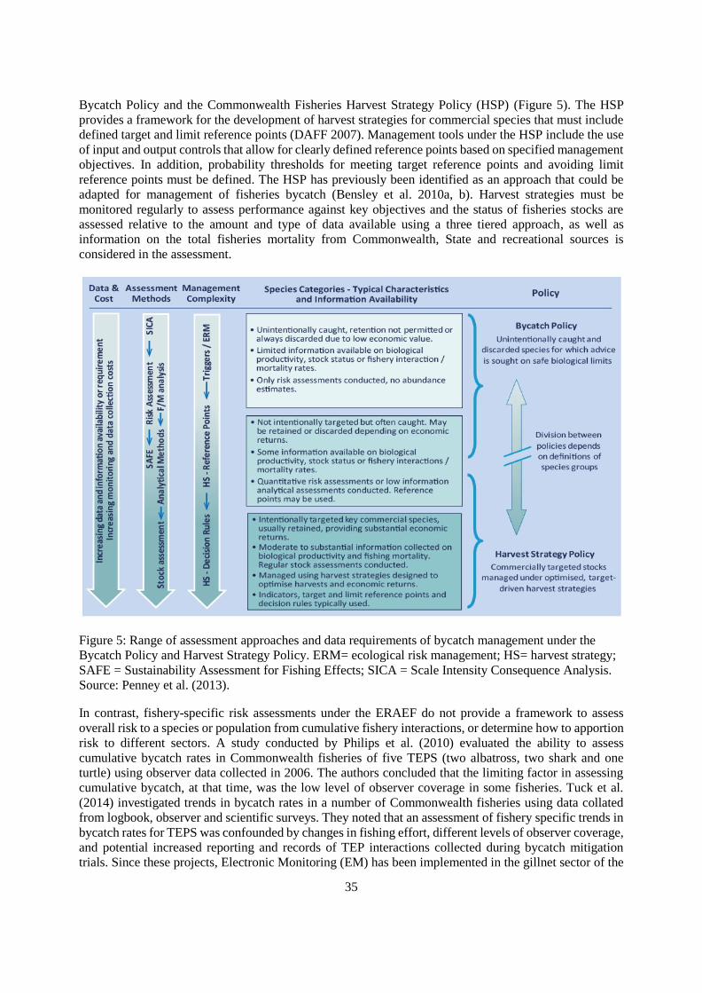
35
Bycatch Policy and the Commonwealth Fisheries Harvest Strategy Policy (HSP) (Figure 5). The HSP
provides a framework for the development of harvest strategies for commercial species that must include
defined target and limit reference points (DAFF 2007). Management tools under the HSP include the use
of input and output controls that allow for clearly defined reference points based on specified management
objectives. In addition, probability thresholds for meeting target reference points and avoiding limit
reference points must be defined. The HSP has previously been identified as an approach that could be
adapted for management of fisheries bycatch (Bensley et al. 2010a, b). Harvest strategies must be
monitored regularly to assess performance against key objectives and the status of fisheries stocks are
assessed relative to the amount and type of data available using a three tiered approach, as well as
information on the total fisheries mortality from Commonwealth, State and recreational sources is
considered in the assessment.
Figure 5: Range of assessment approaches and data requirements of bycatch management under the
Bycatch Policy and Harvest Strategy Policy. ERM= ecological risk management; HS= harvest strategy;
SAFE = Sustainability Assessment for Fishing Effects; SICA = Scale Intensity Consequence Analysis.
Source: Penney et al. (2013).
In contrast, fishery-specific risk assessments under the ERAEF do not provide a framework to assess
overall risk to a species or population from cumulative fishery interactions, or determine how to apportion
risk to different sectors. A study conducted by Philips et al. (2010) evaluated the ability to assess
cumulative bycatch rates in Commonwealth fisheries of five TEPS (two albatross, two shark and one
turtle) using observer data collected in 2006. The authors concluded that the limiting factor in assessing
cumulative bycatch, at that time, was the low level of observer coverage in some fisheries. Tuck et al.
(2014) investigated trends in bycatch rates in a number of Commonwealth fisheries using data collated
from logbook, observer and scientific surveys. They noted that an assessment of fishery specific trends in
bycatch rates for TEPS was confounded by changes in fishing effort, different levels of observer coverage,
and potential increased reporting and records of TEP interactions collected during bycatch mitigation
trials. Since these projects, Electronic Monitoring (EM) has been implemented in the gillnet sector of the

36
SESSF and in the Eastern Tuna and Billfish Fishery (ETBF) and Western Tuna and Billfish Fishery
(WTBF) and as a result should improve the ability to assess cumulative bycatch rates for marine mammal
species in these fisheries. The use of EM will also potentially improve confidence in logbook reporting
rates of TEPS. Fishery-independent observer data are a key source of information required to quantify risk
to TEPS and develop appropriate bycatch reference points.
Noting that data are still lacking to enable fully quantitative estimates of bycatch mortality levels for TEPS
in all Australian fisheries, we propose an additional tier of assessment using existing data be undertaken
as a first step in assessing cumulative impacts of fishing on marine mammal species and/or populations.
This assessment should consider a) spatial distribution of the marine mammal species, b) occurrence of
all fisheries (Commonwealth and State) in the species range, c) type (fishery dependent or independent)
and amount (relative to total fishing effort) of data available on bycatch levels for each fishery, and d) the
level or risk to marine mammal populations from each fishery. Risk of interaction with each fishery would
be assessed in relation to type of fishing gear used, temporal overlap in fishing activities, intensity of
fishing effort, level of previous fishery-independent observer coverage, and information on observed and
reported TEPS interactions. Based on this risk assessment, reference points could then be developed for
each fishery based on the risk assessment, and performance indicators defined to determine if the reference
points were reached.
For widely distributed species, spatial analysis of bycatch across fisheries can provide a means of
identifying areas and/or times of high interaction rates (Goldsworthy and Page 2007, Sims et al. 2008,
Lewison et al. 2014). These data can then be combined with information on the population structure,
movement patterns and temporal densities of the impacted species to develop spatial risk assessments of
bycatch. The use of satellite tags provide direct observations of movement (both longitudinal and inshore-
offshore) that can be used to quantify the risk of fisheries interactions to different populations with respect
to area and season. These data improve spatial risk analyses of the overlap between fishing effort by those
gears assessed as being of high risk to specific populations. The current spatial zones used by AFMA to
manage dolphin interactions in the SPF do not reflect published information on population structure of
SBCD (Möller et al. 2011, Bilgmann et al. 2014a). However, there is evidence that individuals assigned
to different populations can occur in the same spatial area at the same time. For example, a number of
individual SBCD bycaught in South Australian waters in the sardine fishery were assigned to the Pacific
Ocean clade based on their genotype (Bilgmann pers. comm.). Given many populations of marine
mammals are highly mobile, a coordinated approach between Commonwealth and State fisheries
management is needed to assess cumulative bycatch. However, the collection of fishery-independent data
on bycatch rates in fisheries can require significant resources and in some cases it may be more cost
effective to manage a fishery using a precautionary risk based approach rather than invest in more data
collection. Moore et al. (2013) identified that the primary challenge to the development of reference points
was collecting the minimum data required for their development. The move to EM in some
Commonwealth fisheries provides an opportunity to obtain quantitative information on bycatch levels and
assess cumulative impact of bycatch on populations of TEPS in monitored fisheries. Assessments of
strandings data and reports of other sources of mortality such as entanglement in marine debris, direct
killing or ship strike should also be considered.
For small populations, or those with restricted ranges, even low levels of fisheries mortality may be
unsustainable. In these cases abundance data are required to monitor impacts and assess the performance
of bycatch mitigation and management measures. For example, declines of ASL populations in SA have
continued (Goldsworthy et al. 2015a) despite the introduction of extensive management measures to
mitigate bycatch under the Australian Sea Lion Management Strategy (AFMA 2010). There is a need to
revisit population models for this species to assess the extent to which observed declines can be explained
by historical bycatch levels, the timeframe under which recovery as a result of management measures
could be detected, or if there are other factors that may be limiting recovery of this species. For pinniped
populations, abundance data required to assess trends in population are relatively easy to collect,

37
particularly for annual breeding fur seals. In contrast, for cetacean species, such as SBCD, that have large
distributions and exhibit wide-scale movements or migrations, these data require surveys over large areas
that can be costly and logistically challenging. However, such data provide an important reference level
to assess the impact of bycatch or other anthropogenic activities and determine appropriate bycatch limits.
For example, to meet the legislative requirements under the European Union Habitats Directive and inform
conservation and management, wide scale surveys to estimate abundance of small cetaceans in European
waters have been conducted using vessel and aerial surveys (Hammond et al. 2002, 2013). Risk assessment
of bycatch mortality to a population would also be improved by information on the age and sex of
individuals involved. If bycatch is predominantly of reproductively mature females then the impact on
population viability may be greater than if bycatch was directed to males or juveniles. Where data relating
to the life history stages of different populations are scarce, existing archived bycatch samples could be
used to assess the occurrence of different life history stages for populations or species bycaught in
Australian waters. A framework for the collection and utilisation of biological samples from bycaught
animals to inform identification of species, populations, sex and age of bycaught individual was developed
in workshop discussions and provided in Appendix B.
Management of marine mammal interactions with fisheries needs to be adaptive and integrate improved
information on population abundance, trends, bycatch level and/or interaction rates and the effectiveness
of management measures in mitigating interactions. Where management measures have resulted in
reduced fisheries interactions to, or close to zero, but where populations are still declining, identification
of the causes of decline are required, and potential drivers that could further limit population recovery in
the future need to be identified (e.g. environmental changes associated with climate change). For
populations that are increasing as a result of recovery from historical exploitation, exploration of future
population states and identification of areas where interactions with fisheries may increase under various
population trajectories will assist managers and industry to plan and adapt for possible future changes in
interaction levels.
Bensley et al. (2010a, b) recommend a targeted and transparent approach be taken to develop bycatch
management strategies that incorporate reference points, management decision rules and performance
indicators to assess the effectiveness of management approaches. Penny et al. (2013) noted that there
remained a need to develop “measureable and reliable” reference points in Commonwealth fisheries and
proposed a tiered analytical assessment framework be applied to bycatch and byproduct species where the
level of assessment at each tier reflects available data. Fishery-specific reference points should be
developed using available data and spatial risk assessments of the potential cumulative impact of fisheries
bycatch to a given species. Such a method would allow a transparent framework for fishery specific
bycatch reference points to be developed. Performance indicators of management measures can be
assessed relative to these reference points through appropriate levels of representative fisheries
independent monitoring. Monitoring and reporting need to be of adequate quality for the assessment of
mitigation or management performance criteria and for demonstrating that mitigation or management
strategies are achieving their stated management goals. Monitoring also needs to be consistent across
fisheries so that unbiased assessments of the relative risk of different fisheries to a given species can be
made.
As previously concluded by a number of studies (Bensley et al. 2010a, 2010b, Kirby and Ward 2013,
Penney et al. 2013) there remains a need to develop species- and fishery-specific reference points (target
or limit), control rules and performance indicators to manage marine mammal interactions across
Commonwealth and State commercial and recreational fisheries. Reference limits need to be developed
using a process that will be supported by different stakeholder groups and ensure that key management
and policy objectives under key legislation such as the FMA and the EPBC Act can be met by the
Departments responsible for implementing these policies.

38
Conclusion
The project objectives were achieved as follows:
Collate and synthesise all available data on the distribution, abundance and population structure of key
marine mammal species that overlap with the area of the SPF.
Convene an expert workshop to review current information available to inform the establishment of
trigger limits for key marine mammal species (especially the short-beaked common dolphin, and
Australian and long-nosed fur seals) and use structured expert elicitation to assess plausible minimum
population sizes of these species in the area of the SPF.
During the CTW, data relating to the distribution, abundance and population structure of key marine
mammal species were reviewed and discussed. This included a metadata synthesis provided by the
Australian Marine Mammal Centre of State and Commonwealth cetacean sightings and strandings data
available in the National Marine Mammal Database. The review of current information highlighted key
knowledge gaps needed to quantify impacts of fisheries bycatch on protected species, particularly
abundance, distribution and population structure of the small cetacean species considered.
Participants of the CTW agreed that EE is not an appropriate method for obtaining abundance estimates
where empirical data are lacking. Two of the seventeen CTW participants indicated they would not
provide any estimates as part of the EE process and a further three participants did not provide estimates
after the workshop. The total number of individual estimates provided after the second round of EE varied
by species and zones, and EE was only supported for species and/or SPF management zones for which
abundance data were already available. The CTW considered information on the key marine mammal
species in relation to current spatial management zone of the SPF. The appropriateness of these spatial
zones, particularly in relation to managing interactions with highly mobile species, such as SBCD, was
questioned.
Report on the outcomes of the expert workshop and present the results of PBR analyses conducted post-
workshop for short-beaked common dolphins and seals, based on available data, expert opinion and a
precautionary approach.
The project investigated PBR as a means of estimating reference limits for cumulative anthropogenic
mortality to short-beaked common dolphins and seals in the area of the SPF. A key data requirement of
PBR estimation is a recent and robust estimate of abundance. Abundance data for the three pinniped
species considered are relatively good, although recent estimates for ASL are lacking for most breeding
colonies off the south coast of Western Australia. In contrast, abundance data are poor for dolphin species
in Australian waters, and where estimates exist, are mostly restricted to coastal areas or embayments.
Although EE undertaken as part of the CTW provided a means of identifying uncertainties in available
abundance estimates and apportioning those estimates to fishery management zones, it was not used to
provide estimates where no data were available.
The calculation of PBR is relatively simple, but requires a recent estimate of abundance for that population
and that the population is correctly identified. Therefore, caution should be used in interpreting PBR levels
estimated under the current project where some of these factors are either unknown or unresolved.
The PBR limits represent an estimate of the total anthropogenic mortality a population can sustain. These
do not present the estimated limit for a single fishery. PBR levels need to consider cumulative bycatch
across fisheries and jurisdictions, as well as other sources of anthropogenic mortality.

39
Identify knowledge gaps and research needs to improve quantitative robustness of bycatch limit reference
points for each species.
A number of key knowledge gaps were identified during the project that would improve the ability to
estimate bycatch limit reference points for key marine mammal species using a method such as PBR. Key
data gaps for small cetaceans are abundance, distribution and population structure. The collection of
dolphin abundance data, particularly for offshore areas where many Commonwealth fisheries operate,
would require substantial resourcing for aerial and vessel based surveys over larger areas. If interactions
between fisheries and small cetaceans are managed spatially, then improved information on population
structuring and movement patterns are required. The current spatial management of dolphin interactions
in the SPF does not reflect current information relating to these factors for SBCD.
The need to develop a clear and transparent process to determine appropriate bycatch reference points
(both trigger and limit), performance measures and decision rules to manage bycatch of protected species
in Australian commercial fisheries has been identified previously (Bensley et al. 2010a, 2010b, Kirby and
Ward 2013, Penney et al. 2013). This is particularly relevant to managing the potential impact of bycatch
on species that interact with a number of fisheries across jurisdictions. To date, risk assessments for marine
mammals under the ERAEF process have only been conducted to Level 2, and the framework is fishery
specific so does not take into account potential cumulative impacts of fishing and other anthropogenic
mortality to a given population or species. Risk assessments could be improved by inclusion of
quantitative data on bycatch levels across fishery jurisdictions, and should include a spatial bycatch risk
analysis based on the temporal distribution of fishing effort and distribution and relative density of the
bycatch species.
Future setting of fishery specific marine mammal trigger limits should follow a risk assessment approach
that considers the impact of cumulative bycatch across fisheries and jurisdictions. A framework to
determine trigger limits for a population based on relative risk posed by different fisheries should be
implemented to ensure trigger limits reflect assessed levels of bycatch risk. Trigger limits can then be used
as performance indicators within fishery-specific bycatch management plans such as those used by
AFMA.

40
Recommendations
A transparent and consistent approach should be developed to determine appropriate bycatch
trigger limits for marine mammal species in Commonwealth fisheries. This approach should
consider potential cumulative impacts of bycatch and other anthropogenic mortality to a
population for all jurisdictions.
Expert Elicitation is not an appropriate method for calculating Nmin for PBR in the absence of
empirical abundance data. While PBR can be used to estimate sustainable limits of
anthropogenic mortality to a given marine mammal population, the method requires current and
robust estimates of abundance for that population, as well as estimates of total anthropogenic
mortality.
In the absence of information on population size, we recommend that trigger limits should be set
following a risk-based approach that considers the cumulative impact of all Commonwealth and
State fisheries interactions. This assessment should consider a) spatial distribution of the marine
mammal species, b) occurrence of all fisheries (Commonwealth and State) in the species range,
c) type (fishery-dependent or -independent) and amount (relative to total fishing effort) of data
available on bycatch rates for each fishery, and d) level or risk of interaction for each fishery.
The spatial management zones currently used in the Small Pelagic Fishery to manage
interactions with marine mammal species should be reassessed after considering available
information on the population structure and distribution of key species.
There is a need to further investigate the temporal and spatial distribution and population
structure of short-beaked common dolphins.
All bycaught individuals should be identified to species level and validated with photographs,
whether through fishery dependent logbooks or fishery independent monitoring. Current fishery
logbook reports often only record taxa level information for the interaction (e.g. seal or
dolphin).

41
References
Full text of the U.S. Marine Mammal Protection Act (1994) available at:
http://www.nmfs.noaa.gov/pr/laws/mmpa/text.htm#section3
Adams-Hosking, C., McBride, M. F., Baxter, G., Burgman, M., de Villiers, D., Kavanagh, R., Lawler, I.,
Lunney, D., Melzer, A., Menkhorst, P., Molsher, R., Moore, B. D., Phalen, D., Rhodes, J. R., Todd, C.,
Whisson, D. and McAlpine, C. A. (2015). Use of expert knowledge to elicit population trends for the koala
(Phascolarctos cinereus). Diversity and Distributions. doi:10.1111/ddi.12400
AFMA (2008). Program for Addressing Bycatch and Discarding in Commonwealth fisheries implementation
strategy. http://www.afma.gov.au/wp-content/uploads/2014/11/Bycatch-and-Discarding-Implementation-
Strategy-feb-08.pdf
AFMA (2010a). Ecological Risk Management. Report for the midwater trawl sector of the Small pelagic
Fishery http://www.afma.gov.au/wp-content/uploads/2014/11/Ecological-Risk-Management-SPF-midwater-
trawl-March-2010.pdf
AFMA (2010b). Australian Sea Lion Management Strategy. Southern and eastern Scalefish and Shark
Fishery. Version 2.0 – updated July 2015.
AFMA (2014a). Small Pelagic Fishery, Bycatch and Discarding Workplan. 2014-2016.
http://www.afma.gov.au/wp-content/uploads/2014/11/Bycatch-and-Discard-Work-Plan-SPF-2016.pdf
AFMA (2014b). Dolphin Strategy, minimising gillnet bycatch, September 2014.
http://www.afma.gov.au/wp-content/uploads/2014/02/AFMA-Dolphin-Strategy-September-2014.pdf
AFMA (2015a). Vessel Management Plan (VMP) Small Pelagic Fishery, Geelong Star. September 2015.
Version 1.5. http://www.afma.gov.au/wp-content/uploads/2015/09/Vessel-Management-Plan1.5.pdf
AFMA (2015b). Small Pelagic Fishery Management Arrangements Booklet 2015-16. Australian Fisheries
Management Authority. Canberra, Australia.
Archer, F., Gerrodette, T., Chivers, S. and Jackson, A. (2004). Annual estimates of the unobserved incidental
kill of pantropical spotted dolphin (Stenella attenuata attenuata) calves in the tuna purse-seine fishery of the
eastern tropical Pacific. Fishery Bulletin, 102 (2), 233-244.
Arnould, J.P.Y. and Kirkwood, R. (2008). Habitat selection in a benthic diver: the foraging areas of female
Australian fur seals (Arctocephalus pusillus doriferus). Aquatic Conservation: Marine and Freshwater
Ecosystems 17, S53–S67.
Baird, R.W., Webster, D.L, Swaim, Z, Foley, H.J., Anderson, D.B. and Read, A.J. (2015a). Spatial Use by
Cuvier’s Beaked Whales, Short-finned Pilot Whales, Common Bottlenose Dolphins, and Short-beaked
Common Dolphins Satellite Tagged off Cape Hatteras, North Carolina, in 2014. Draft Report. Prepared for
U.S. Fleet Forces Command. Submitted to Naval Facilities Engineering Command Atlantic, Norfolk,
Virginia, under Contract No. N62470-10-3011, Task Orders 14 and 21, issued to HDR Inc., Virginia Beach,
Virginia. 17 July 2015.
Baird, R. W., Mahaffy, S. D., Gorgone, A. M., Cullins, T., McSweeney, D. J., Oleson, E. M., Bradford, A.
L., Barlow, J. and Webster, D. L. (2015b). False killer whales and fisheries interactions in Hawaiian waters:
Evidence for sex bias and variation among populations and social groups. Marine Mammal Science,
31: 579–590.
Bensley, N, Stobutzki, I, Woodhams, J and Mooney, C (2010a). Review of wildlife bycatch management in
Commonwealth fisheries, BRS report prepared for the Department of Agriculture, Fisheries & Forestry,
Fisheries Policy Branch, Canberra, July.

42
Bensley, N, Stobutzki I and Begg, G (2010b). An integrated approach to wildlife bycatch: addressing key
issues to progress the implementation of national plans of action, BRS report prepared for the Department of
Agriculture, Fisheries and Forestry, Canberra, July.
Bilgmann, K, Parra, G.J. and Möller, L.M. (2014a). Inshore cetacean survey between Ceduna and Coffin
Bay, eastern Great Australian Bight. Report as part of the Great Australian Bight Research Program.
Bilgmann, K., Parra, G.J., Zanardo, N., Beheregaray, L.B., and Möller, L.M (2014b). Multiple management
units of short-beaked common dolphins subject to fisheries bycatch off southern and southeastern Australia.
Marine Ecology Progress Series. 500: 265-279
Brown, S., Reid, D. and Rogan, E. (2014). Characteristics of fishing operations, environment and life history
contributing to small cetacean bycatch in the Northeast Atlantic. PLOS One. 9(8): e104468.
Caddy, J.F. and Mahon, R. (1995). Reference points for fisheries management. FAO Fisheries Technical
Paper. No. 347. Rome, FAO. 83pp.
Campbell, R.A., Gales, N.J., Lento, G.M. and Baker, C.S. (2008). Islands in the sea: extreme female natal
site fidelity in the Australian sea lion, Neophoca cinerea. Biology Letters 4, 139–142.
Campbell R. (2011). Assessing and managing interactions of protected and listed marine species with
commercial fisheries in Western Australia. Report to the Fisheries Research and Development Corporation.
Fisheries Research report No.223. Department of Fisheries, Western Australia. 48pp.
Campbell, R., Holley, D., Collins, P. and Armstrong, S. (2014). Changes in the abundance and distribution of
the New Zealand fur seal (Arctocephalus forsteri) in Western Australia: are they approaching carrying
capacity? Australian Journal of Zoology, 62: 261–267
Carretta, J.V., Oleson, E.M., Baker, J., Weller, D.W., Lang, A.R., Forney, K.A., Muto, M.M, Hanson, B.,
Orr, A.J., Huger, H., Lowry, M.S., Barlow, J., Moore, J.E., Lynch, D., Carswell, L. and Brownell, R.L.
(2016). U.S. Pacific Marine Mammal Stock Assessments 2015. NOAA Technical Memorandum NMFS.
doi:10.7289/V5/TM-SWFSC-561.
Charlton-Robb, K., Gershwin, L.A., Thompson, R., Austin, J., Owen, K. and McKechnie, S. (2011). A New
Dolphin Species, the Burrunan Dolphin Tursiops australis sp. nov., Endemic to Southern Australian Coastal
Waters. PLoS ONE. 6(9): e2404.
Charlton-Robb, K., Taylor, A.C. and McKechnie, S.W. (2014). Population genetic structure of the Burrunan
dolphin (Tursiops australis) in coastal waters of south-eastern Australia: conservation implications.
Conservation Genetics 16 (1): 195-217.
Cockcroft, V.G. and Peddemors, V.M. (1990). Seasonal distribution and density of common dolphins
Delphinus delphis off the south-east coast of Southern Africa. South African Journal of Marine Science.
9:371-377
Commonwealth of Australia (2014). Threat Abatement Plan 2014 for the incidental catch (or bycatch) of
seabirds during oceanic longline fishing operations, Department of the Environment, Canberra.
Curtis, K.A., Moore, J.E., Boyd, C. Dillingham, P.W., Lewison, R.L., Taylor, B.L and James, K.C. (2015).
Managing catch of marine megafauna: Guidelines for setting limit reference points. Marine Policy. 61:249-
263
Cribb, N., Miller, C. and Seuront, L. (2013). Indo-Pacific bottlenose dolphin (Tursiops aduncus) habitat
preference in a heterogeneous, urban, coastal environment. Aquatic Biosystems. 9:3.
Department of Agriculture, Fisheries and Forestry (2007). Commonwealth Fisheries Harvest Strategy. Policy
and Guidelines http://www.agriculture.gov.au/SiteCollectionDocuments/fisheries/domestic/hsp.pdf
Department of Agriculture, Fisheries and Forestry (2013). Report on the review of the Commonwealth
Policy on Fisheries Bycatch, Department of Agriculture, Fisheries and Forestry, Canberra.

43
Daley, R., Dowdney, J., Bulman, C, Sporcic, M., Fuller, M., Ling, S. and Hobday, A (2007). Ecological Risk
Assessment for the Effects of Fishing. Report for the midwater trawl sub-fishery of the Small Pelagic
Fishery. Report for the Australian Fisheries Management Authority. Canberra, Australia.
Dennis, T. E. and Shaughnessy, P. D. (1996). Status of the Australian sea lion, Neophoca cinerea, in the
Great Australian Bight. Wildlife Research, 23: 741-754.
Expert Panel on a Declared Commercial Fishing Activity (2014). Report of the Expert Panel on a Declared
Commercial Fishing Activity: Final (Small Pelagic Fishery) Declaration 2012.
Fernández-Contreras, F.F, Cardona, L., Lockyer C. H., and Aguilar, A. (2010). Incidental bycatch of short-
beaked common dolphins (Delphinus delphis) by pairtrawlers off northwestern Spain. ICES Journal of Marine
Science, 67: 1732–1738.
Filby, N.E., Bossley, M., Sanderson, K.J., Martinez, E. and Stockin, K.A. (2010). Distribution and
population demographics of common dolphins (Delphinus delphis) in the Gulf St. Vincent, South Australia.
Aquatic Mammals, 36(1): 33-45
Fitzgerald, J., Ashby, C. and Buxton, C., (Eds.) (2015). 2014-046 Small Pelagic Research Coordination
Program: Technical workshop to explore options for mitigating marine mammal interactions in the Small
Pelagic Fishery.
Gales, N. J., Shaughnessy, P. D. and Dennis, T. E. (1994). Distribution, abundance and breeding cycle of the
Australian sea lion, Neophoca cinerea (Mammalia: Pinnipedia). Journal of Zoology, London, 234: 353-370.
Gerrodette, T. and Forcada, J. (2005). Non-recovery of two spotted and spinner dolphin populations in the
eastern tropical Pacific Ocean. Marine Ecology Progress Series. 291: 1-21.
Goldsworthy, S. D. and Page, B. (2007). A Risk-Assessment Approach to Evaluating the Significance of Seal
Bycatch in two Australian Fisheries. Biological Conservation, 139: 269-285.
Goldsworthy, S. D., Page, B., Shaughnessy, P. D. and Linnane, A. (2010). Mitigating seal interactions in the
SRLF and the gillnet sector SESSF in South Australia. FRDC Project 2007/041 Final Report. SARDI Aquatic
Sciences Publication Number F2009/000613-1, SARDI Research Report Series Number 405, 213 pp.
Goldsworthy, S.D., Mackay, A.I., Shaughnessy, P.D., Bailleul, F. and Holman, D (2015a). Maintaining the
monitoring of pup production at key Australian sea lion colonies in South Australia (2014/15). Final Report
to the Australian Marine Mammal Centre. South Australian Research and Development Institute (Aquatic
Sciences), Adelaide. SARDI Publication No. F2012/000665-5. SARDI Research Report Series No. 871.
73pp.
Goldsworthy, S. D., Bailleul, F., Shaughnessy, P. D., Kennedy, C., Stonnill, M., Lashmar, K., Mackay, A. I.
and McMahon, C. (2015b). Monitoring of Seal Bay and other pinniped populations on Kangaroo Island:
2014/2015. Report to the Department of Environment, Water and Natural Resources. South Australian
Research and Development Institute (Aquatic Sciences), Adelaide. SARDI Publication No. F2014/000332-2.
SARDI Research Report Series No. 881. 48pp
Hall, M.A. (1998). An ecological view of the tuna-dolphin problem: impacts and trade-offs. Reviews in Fish
Biology and Fisheries, 8: 1-34.
Hammond, P.S., Berggren, P., Benke, H., Borchers, D.L., Collet, A., Heide-Jørgensen, M.P, Heimlich, S.,
Hiby, A.R., Leopold, M.F, Øien, N. (2002) Abundance of harbour porpoises and other cetaceans in the North
Sea and adjacent waters. Journal of Applied Ecology. 39: 361-376
Hammond, P.S., Macleod, K., Berggren, P., Borchers, D.L., Burt, L., Cañadas, A., Desportes, G., Donovan,
G.P., Gilles, A., Gillespie, D., Gordon, J., Hiby, L., Kuklik, I., Leaper, R., Lehnert, K., Leopold, M., Lovell,
P., Øien, N., Paxton, C.G.M, Ridoux, V., Rogan, E., Samarra, F., Scheidat, M., Sequeira, M., Siebert, U.,
Skov, H., Swift, R., Tasker, M.L., Teilmann, J., Van Canneyt, O., Vázquez, J.A. (2013). Cetacean abundance
and distribution in European Atlantic shelf waters to inform conservation and management, Biological
Conservation, 164: 107-122.

44
Hobday, A.J., Smith, A.D.M., Webb, H., Daley, R., Wayte, S., Bulman, C., Dowdney, J., Williams, A.,
Sporcic, M., Dambacher, J., Fuller, M. and Walker, T. (2007). Ecological Risk Assessment for the Effects of
Fishing: Methodology. Report R04/1072 for the Australian Fisheries Management Authority, Canberra. July
2007. Available from: http://www.afma.gov.au/environment/eco based/ eras/docs/methodology.pdf.
Hobday, A.J., Smith, A.D.M., Stobutzki, I.C., Bulman, C., Daley, R., Dambacher, J.M., Deng, R.A.,
Dowdney, J., Fuller, M., Furlani, D., Griffiths, S.P., Johnson, D., Kenyon, R., Knuckey, I.A., Ling, S.D.,
Pitcher, R., Sainsbury, K.J., Sprocic, M., Smith, T., Turnbull, C., Walker, T.I., Wayte, S.E., Webb, H.,
Williams, A., Wise, B.S. and Zhou, S. (2011). Ecological risk assessment for the effects of fishing. Fisheries
Research. 108: 372-384
ICES (2013). Report of the Working Group on Marine Mammal Ecology (WGMME), 4– 7 February 2013,
Paris, France. ICES CM 2013/ACOM: 26. 117 pp.
Kemper, C., Coughran, D., Warneke, R., Pirzl, R., Watson, M., Gales, R. and Gibbs, S. (2008). Southern
right whale (Eubalaena australis) mortalitites and human interactions in Australia, 1950-2006. Journal of
Cetacean Research and Mangement. 10(1): 1-8
King, S. L., Schick, R. S., Donovan, C., Booth, C. G., Burgman, M., Thomas, L., Harwood, J. (2015). An
interim framework for assessing the population consequences of disturbance. Methods in Ecology and
Evolution, 6: 1150–1158.
Kirkwood, R. and Arnould, J.P.Y. (2011). Foraging trip strategies and habitat use during late pup rearing by
lactating Australian fur seals. Australian Journal of Zoology. 59: 216–226.
Lancaster, M. L., Arnould, J. P. Y., and Kirkwood, R. (2010). Genetic status of an endemic marine mammal,
the Australian fur seal, following historical harvesting. Animal Conservation 13, 247–255.
Lawson, .J.W., Gosselin, J.F. (2009). Distribution and preliminary abundance estimates for cetaceans seen
during Canada’s marine megafauna survey A component of the 2007 TNASS. Report to the Canadian
Science Advisory Secretariat Department of Fisheries and Oceans. 28 pages.
Lewison, R. L., L. B. Crowder, B. P. Wallace, J. E. Moore, T. Cox, R. Zydelis, S. McDonald, A. DiMatteo,
D. C. Dunn, C. Y. Kot, R. Bjorkland, S. Kelez, C. Soykan, K. R. Stewart, M. Sims, A. Boustany, A. J. Read,
P. Halpin, W. J. Nichols and C. Safina (2014). "Global patterns of marine mammal, seabird, and sea turtle
bycatch reveal taxa-specific and cumulative megafauna hotspots." Proceedings of the National Academy of
Sciences 111(14): 5271-5276.
Ling, J.K. and Walker, G.E. (1978). An 18-month breeding cycle in the Australian sea lion? Search 9,
464−465.
Lowther, A.D., Harcourt, R.G., Goldsworthy, S.D., & Stow, A. (2012). Population structure of adult female
Australian sea lions is driven by fine-scale foraging site fidelity. Animal Behaviour 83, 691–701.
Martin, T., Burgman, M., Fidler, F., Kuhnert, P., Low-Choy, S., McBride, M. and Mengersen, K. (2012).
Eliciting Expert Knowledge in Conservation Science. Conservation Biology, 26, 29–38.
McBride, M. F., Garnett, S. T., Szabo, J. K., Burbidge, A. H., Butchart, S. H. M., Christidis, L., Dutson, G.,
Ford, H. A., Loyn, R. H., Watson, D. M. and Burgman, M. A. (2012). Structured elicitation of expert
judgments for threatened species assessment: a case study on a continental scale using email. Methods in
Ecology and Evolution, 3: 906–920.
McIntosh, R., Sutherland, D., Dann, P., Kirkwood, R., Thalman, S., Alderman, R., Arnould, J.P., Mitchell,
T., Kirkman, S.P., Salton, M., Slip, D. (2014). Pup estimates for Australian and new Zealand fur seals in
Victoria, Tasmania and New South Wales between 2007 and 2013. Report to The Australian Marine
Mammal Centre, Department of the Environment.
Mendez, M., Rosenbaum, H.C., Wells, R.S., Stamper, A. and Bordino, P. (2010). Genetic evidence
highlights potential impacts of by-catch to cetaceans, PLoS ONE 5(12):e15550

45
Möller L.M., Allen S.J. and Harcourt R.G. (2002). Group characteristics, site fidelity and seasonal
abundance of bottlenose dolphins Tursiops aduncus in Jervis Bay and Port Stephens, southeastern Australia.
Australian Mammalogy 24: 11-21.
Möller, L. Valdez, F.P., Allen, S., Bilgmann, K., Corrigan, S. and Beheregaray, L.B (2011). Fine-scale
genetic structure in short-beaked common dolphins (Delphinus delphis) along the East Australian Current.
Marine Biology. 158:113-126
Möller, L., Parra, G.J. and Bilgmann, K. (2012). Population size, structure and habitat preferences of
common dolphins in South Australia: enhancing the assessment, reduction and mitigation of fisheries
operational interactions. Final report to the Australian Marine Mammal Centre.
Moore, J.E., Curtis, K.A., Lewison, R.L., Dillingham, P.W., Cope, J.M., Fordham, S.V., Heppell, S.S.,
Pardo, S.A., Simpfendorfer, C.A., Tuck, G.N. and Zhou, S. (2013). Evaluating sustainability of fisheries
bycatch mortality for marine megafauna: a review of conservation reference points for data-limited
populations. Environmental Conservation. 40 (4): 329-344
Morgan, M.G. (2014). Use (and abuse) of expert elicitation in support of decision making for public policy.
Proceedings of the National Academy of Sciences of the United States of America. 111(20):7176-7184
Moura, A.E., Natoli, A., Rogan, E. and Hoelzel, R. (2013). Atypical panmixia in a European dolphin species
(Delphinus delphis): implications for the evolution of diversity across oceanic boundaries. Journal of
Evolutionary Biology. 26(1): 63-75.
Munto, M.M., Helker, V.T., Angliss, R.P., Allen, B.A., Boveng, P.L., Breiwick, J.M., Cameron, M.F.,
Clapham, P.J, Dahle, S.P., Dahlheim, M.E., Fadely, B.S., Ferguson, M.C., Fritz, L.W., Hobbs, R.C.,
Ivashchenko, Y.V., Kennedy, A.S., London, J.M., Mizroch, S.A., Ream, R.R., Richmond, E.L., Shelden,
K.E.W., Towell, R.G., Wade, P.R., Waite, J.M. and Zerbini, A.R. (2015). Alaska marine mammal stock
assessments, 2015. U.S.Dep. Commer., NOAA Tech. Memo. NMFS-AFSC-323, 300p.
Murphy, S., Pinn, E. H. and Jepson, P.D. (2013). The short-beaked common dolphin (Delphinus delphis) in
the North-East Atlantic: distribution, ecology, management and conservation status. Oceanography and
Marine Biology: An Annual review. 51: 193-280
National Marine Fisheries Service (2016). Guidelines for preparing stock assessment reports pursuant to the
1994 amendments to the MMPA. Protected Resources Management Marine Mammal Protection Act –
Procedures. National Marine Fisheries Service Instruction 02-204-01. February 22, 2016.
http://www.nmfs.noaa.gov/pr/sars/pdf/gamms2016.pdf
Oedekoven, C. Fleishman, E., Hamilton, P., Clark, J.S. and Schick, R.S. (2015). Expert elicitation of
seasonal abundance of North Atlantic right whales Eubalaena glacialis in the mid-Atlantic. Endangered
Species Research. 29: 51-58
Page, B. McKenzie, J., McIntosy, R., Baylis, A., Morrissey, A., Calvert, N., Haase, T., Berris, M., Dowie,
D., Shaughnessy, P.D. and Goldsworthy, S.D. (2004). Entanglement of Australian sea lions and New
Zealand fur seals in lost fishing gear and other marine debris before and after Government and industry
attempts to reduce the problem. Marine Pollution Bulletin. 49:33-42
Page, B., McKenzie, J., Sumner, M.D., Coyne, M. and Goldsworthy, S.D. (2006). Spatial separation of
foraging habitats among New Zealand fur seals. Marine Ecology Progress Series 323, 263–279.
Palka, D. (2012). Cetacean abundance estimates in US northwestern Atlantic Ocean waters from summer
2011 line transect survey. US Dept Commer, Northeast Fish Sci Cent Ref Doc. 12-29; 37 p. Available from:
National Marine Fisheries Service, 166 Water Street, Woods Hole, MA 02543-1026, or online at
http://www.nefsc.noaa.gov/ nefsc/publications/
Philips, K, Giannini, F, Lawrence, E and Bensley, N (2010). Cumulative assessment of the catch of non-
target species in Commonwealth fisheries: a scoping study, Bureau of Rural Sciences, Canberra

46
Shaughnessy, P.D., Briggs, S.V., and Constable, R. (2001). Observations on seals at Montague Island, New
South Wales. Australian Mammalogy 23: 1-7.
Shaughnessy, P. D., Goldsworthy, S. D., Mackay, A.I. (2015). The long-nosed fur seal (Arctocephalus
forsteri) in South Australia in 2013-14: abundance, status and trends. Australian Journal of Zoology, 63:101-
110.
Sims, M., Cox, T. and Lewison, R. (2008). Modeling spatial patterns in fisheries bycatch: improving bycatch
maps to aid fisheries management. Ecological Applications. 18(3): 649-661.
Smith, H.C., Pollock, K., Waples, K., Bradley, S. and Bejder L. (2013). Correction: Use of the Robust
Design to Estimate Seasonal Abundance and Demographic Parameters of a Coastal Bottlenose Dolphin
(Tursiops aduncus) Population. PLOSOne. http://dx.doi.org/10.1371/journal.pone.0076574
Tilzey, R.D.J., Goldsworthy, S., Cawthorn, M., Calvert, N., Hamer, D., Russell, S., Shaughnessy, P.D.,
Wize, B. and Stewardson, C. (2006). Assessment of seal-fishery interactions in the winter blue grenadier
fishery off west Tasmania and the development of fishing practices and Seal Exclusion Devices to mitigate
seal bycatch by factory trawlers.’ FRDC Project No. 2001/008 Final Report. Bureau of Rural Sciences,
Canberra.
Wade, P.R. (1998). Calculating limits to the allowable human-caused mortality of Cetaceans and Pinnipeds.
Marine Mammal Science. 14:1–37.
Wade, P.R., Watters, G.M., Gerrodette, T. and Reilly, S.B. (2007). Depletion of spotted and spinner dolphins
in the eastern tropical Pacific: modelling hypotheses for their lack of recovery. Marine Ecology Progress
Series. 343: 1-14.
Ward, T.M., Ivey, A., Burnell, O. and Carroll, J. (2015). Effectiveness of the industry Code of Practice in
mitigating operational interactions of the South Australian Sardine Fishery with the short-beaked common
dolphin (Delphinus delphis) Report to PIRSA Fisheries and Aquaculture. South Australian Research and
Development Institute (Aquatic Sciences), Adelaide. SARDI Publication No. F2010/000726-5. SARDI
Research Report Series No. 821. 35pp.
Waring, G.T., Josephson, E., Maze-Foley, K. and Rosel, P.E. (Eds) (2015). US Atlantic and Gulf of Mexico
Marine mammal Stock Assessments – 2015. NOAA Technical Memorandum NMFS-NE-238
Woinarski, J.C.S, Burbidge, A.A. and Harrison, P.L (2012). The Action Plan for Australian Mammals 2012.
CSIRO Publishing. Melbourne.
Zagzebski, K.A., Gulland, F.M.D, Haulena, M., Lander, M.E., Greig, D.J., Gage, L.J., Bradley Hanson, M.,
Yochem, P.K. and Stewart, B.S. (2006). Twenty-Five Years of Rehabilitation of Odontocetes Stranded in
Central and Northern California, 1977 to 2002.Aquatic Mammals 2006, 32(3), 334-345

Appendix A Report on the Closed Technical Workshop and Expert Elicitation Process under the project Eliciting Expert
Knowledge to inform the establishment of trigger limits for key marine mammal species that overlap with the
Commonwealth Small Pelagic Fishery (SPF)
Alice I. Mackay, Simon D. Goldsworthy & Peter Harrison
February 2016
FRDC Project No. 2015/035
48
Contents
Appendix A ............................................................................................................................................ 1
Contents ................................................................................................................................................ 48
Tables .................................................................................................................................................... 49
Introduction ......................................................................................................................................... 51
Objectives ............................................................................................................................................. 52
Method .................................................................................................................................................. 53
Synthesis of available information on key marine mammal species that overlap with the SPF . 57
Australian sea lion (Neophoca cinerea) ......................................................................................... 57
Long-nosed fur seal (Arctocephalus forsteri) – formerly New Zealand fur seal ........................... 59
Australian fur seal (Arctocephalus pusillus doriferus) ................................................................... 61
Short-beaked common dolphin (Delphinus delphis) ...................................................................... 62
Bottlenose dolphin (Tursiops sp.) ................................................................................................... 65
Results of Expert Elicitation .............................................................................................................. 67
Elicited estimates of Nmin for Australian sea lion (ASL) abundance .............................................. 67
Elicited estimates of Nmin for long-nosed fur seal (LNFS) abundance ........................................... 69
Elicited estimates of Nmin for Australian fur seal (AUFS) abundance ............................................ 71
Elicited estimates of Nmin for short-beaked common dolphin (SBCD) abundance ........................ 72
Elicited estimates of Nmin for coastal bottlenose dolphins .............................................................. 73
Discussion ............................................................................................................................................. 75
Estimates of abundance from expert elicitation.............................................................................. 75
Feedback on elicitation method and application of workshop outcomes ....................................... 79
Knowledge gaps identified during the closed technical workshop. ............................................... 79
References ............................................................................................................................................ 82
Appendix B: CEBRA report on the Expert Elicitation Process ..................................................... 87
Appendix C: AMMC data synthesis report ...................................................................................... 88
Appendix D: Framework for the collection of biological data ....................................................... 89
Appendix E: Workshop Agenda ........................................................................................................ 91

49
Tables
Table 1: Published estimates of Australian sea lion pup abundance in the area of the Small Pelagic Fishery considered by participants of the Closed Technical Workshop. ......................................................................59
Table 2: Published estimates of long-nosed fur seal pup abundance in the area of the Small Pelagic Fishery considered by participants of the Closed Technical Workshop. ......................................................................61
Table 3: Published estimates of Australian fur seal pup abundance in the area of the Small Pelagic Fishery considered by participants of the Closed Technical Workshop. ......................................................................62
Table 4: Published estimates of short-beaked common dolphin abundance in the area of the Small Pelagic Fishery considered by participants of the Closed Technical Workshop. *estimated by multiplying density estimate by area of Gulf St Vincent with depth > 14m. **Conventional Distance Sampling (CDS). ***Multiple covariate distance sampling (MCDS) ..........................................................................................63
Figures
Figure 1a: The two sub-areas (east and west of Tasmania indicated by the red line) and seven management zones of the Small Pelagic Fishery. Source (AFMA 2015) ............................................................................54
Figure 1b – spreadsheet provided to workshop participants during teleconference. .......................................55
During the teleconference Dr Carey provided a general description of CEBRA’s structured elicitation process, including the influence of cognitive biases and the steps employed to counter their effects. ...........56
Figure 2a: Distribution of Australian sea lion breeding colonies in the SPF area. ..........................................58
Figure 2b: Distribution of long-nosed fur seal breeding colonies in the SPF area. .........................................58
Figure 2c: Distribution of Australian fur seal breeding colonies in the SPF area. ..........................................58
Figure 3: Spatial management zones 1 and 2 considered during the second round of expert Elicitation for the estimation of Australian sea lion abundance. ...................................................................................................67
Figure 4: Individual expert and group best estimates of Australian sea lion abundance for Zone 1 from the second round of expert elicitation. Bars represent estimates of lowest and highest plausible estimates of abundance adjusted to the confidence levels experts provided with their estimates. ......................................68
Figure 5: Individual expert and group best estimates of Australian sea lion abundance for Zone 2 from the second round of expert elicitation. Bars represent estimates of lowest and highest plausible estimates of abundance adjusted to the confidence levels experts provided with their estimates. Elicited estimates of Nmin for long nosed fur seal abundance ....................................................................................................................68
Figure 6: The three spatial management zones considered during the second round of expert elicitation for the estimation of long-nosed fur seal abundance. ............................................................................................69
Figure 7: Individual expert and group estimates of lowest long-nosed fur seal abundance in Zone 1 from the second round of expert elicitation. Confidence intervals represent derived 80% confidence adjusted from the confidence levels experts provided with their estimates. .................................................................................70
Figure 8: Individual expert and group best estimates of long-nosed fur seal abundance in Zone 2 from the second round of expert elicitation. Bars represent estimates of lowest and highest plausible estimates of abundance adjusted to the confidence levels experts provided with their estimates. ......................................70
Figure 9: Individual expert and group best estimates of long-nosed fur seal abundance in Zone 3 from the second round of expert elicitation. Bars represent estimates of lowest and highest plausible estimates of abundance adjusted to the confidence levels experts provided with their estimates. ......................................71
50
Figure 10: Management Zone 1 considered during the second round of expert elicitation for the estimation of Australian fur seal abundance. .....................................................................................................................71
Figure 11: Individual expert and group best estimates of Australian fur seal abundance in Zone 1 from the second round of expert elicitation. Bars represent estimates of lowest and highest plausible estimates of abundance adjusted to the confidence levels experts provided with their estimates. ......................................72
Figure 12: The seven bycatch management zones used by AFMA to manage dolphin interactions within the SPF. ..................................................................................................................................................................72
Figure 13: Individual expert and group best estimates of short-beaked common dolphin in Zone 3 from the second round of expert elicitation. Bars represent estimates of lowest and highest plausible estimates of abundance adjusted to the confidence levels experts provided with their estimates. ......................................73
Figure 14: Average group best estimates for inshore bottlenose dolphin abundance across all bycatch management zones and subregions during the second round of expert elicitation. Bars represent average group estimates of lowest and highest plausible estimates of abundance ........................................................74

51
Introduction
This document provides the methods and results of a closed technical workshop (CTW) convened at SARDI Aquatic Sciences on 20 October 2015. The aims of the CTW were for invited experts to a) review and discuss available data on key marine mammal species that overlap with the area of the Small Pelagic Fishery (SPF), b) identify data gaps and research needs for each species, c) provide minimum, maximum and best estimates of population numbers through expert elicitation (EE) and d) provide feedback on the elicitation process and outcomes.
These aims addressed the recommendations of the report of a technical workshop convened by the Fisheries Research and Development Corporation (FRDC) in Melbourne, Victoria, on 25-26 June 2015 (Fitzgerald et al. 2015). That workshop identified uncertainty as to the methods and data used to derive marine mammal trigger limits in the SPF, and to determine the duration of the temporal closures of management zones in response to dolphin bycatch events (Fitzgerald et al. 2015). A key recommendation from the workshop was that “An expert group should be established to review current information available to inform the establishment of trigger limits for key marine mammal species (especially the short-beaked common dolphin, Australian fur seals and long-nosed fur seals)” (Fitzgerald et al. 2015). Specifically the report stated that “The workshop agreed that in the absence of a robust scientific assessment of dolphin numbers in the area of the SPF, a precautionary approach to setting trigger limits for the incidental bycatch of dolphins was appropriate. In the short term, an assessment of plausible minimum population sizes could be made based on currently available information and expert judgement”. The recommendation was that an expert group would develop “initial estimates of the minimum population size of key [marine mammal] species in each fishing zone and if possible the area of the fishery” to be used to calculate “Potential Biological Removals (PBR) that would ensure that the population viability of marine mammals…..is not compromised by fishing-mortality from the SPF”.
Expert elicitation was chosen as a method to synthesise expert judgement as it can be used to collate expert opinion in situations where empirical data are limited but a need exists to qualify or quantify risk (Martin et al. 2012, McBride et al. 2012). For example, structured expert elicitation has been used to assess the IUCN Red list category of extinction risk for selected Australian bird taxa (McBride et al. 2012), estimate abundance and trends of koala populations (Adams-Hosking et al. 2016), to estimate the effect of anthropogenic disturbance on harbour porpoises (Phocoena phocoena) as inputs into a stochastic population model (King et al. 2015), and to identify global bycatch hotspots for seabirds, marine mammals and turtles (Lewison et al. 2014).
The Ecological Risk Assessment of the Effects of Fishing (ERAEF) (Hobday et al. 2007) for mid-water trawl fisheries in the SPF identified 23 marine mammal species as high risk using Productivity Susceptibility Analysis (PSA) (Daley et al. 2007). The residual risk analysis of the Level 2 PSA which considers management measures in the fishery retained eight marine mammal species as high risk (AFMA 2010a). The CTW considered three of these eight species; the Australian fur seal (Arctocephalus pusiilus doriferus) the bottlenose dolphin (Tursiops truncatus), and the Indian Ocean bottlenose dolphin (Tursiops aduncus). The CTW did not consider the other five small cetacean species identified as at high risk during the PSA of the ERAEF (Daley et al. 2007) as there is no information on the distribution and abundance of these species and there have been no recorded interactions between these species and mid-water trawl operations in the SPF.
In addition, the CTW considered the short-beaked common dolphin (SBCD) (Delphinus delphis) and long-nosed fur seal (LNFS) (Arctocephalus forsteri – formerly New Zealand fur seal), based on the recommendation by Fitzgerald et al. (2015) and on recorded bycatch of SBCD and fur seals in the fishery. Both species were also identified as at medium risk after residual risk analysis (AFMA 2010a). Australian sea lions (ASL) (Neophoca cinerea), were considered as part of the assessment based on the Report of the Expert Panel on a Declared Commercial Fishing Activity: Final (Small Pelagic Fishery) Declaration 2012 (2014), which identified that there was a risk of direct interactions between ASL and midwater trawls as 95% of the species’ range is adjacent to the area of the SPF.

52
Objectives
This report synthesises available data on marine mammal species that overlap with the SPF and reports on the results of a CTW to provide estimates of lowest plausible abundances for these species.
The specific aims addressed the recommendations outlined in Fitzgerald et al. (2015) and were as follow:
• Collate and synthesise all available data on the distribution, abundance and population structure of
key marine mammal species that overlap with the area of the SPF.
• Convene an expert workshop to review current information available to inform the establishment of
trigger limits for key marine mammal species (especially the short-beaked common dolphin, and
Australian and long-nosed fur seals) and use structured expert elicitation to assess plausible
minimum population sizes of these species in the area of the SPF.
• Identify knowledge gaps and research needs to improve quantitative robustness of bycatch limit
reference points for each species.
53
Method
Recent published literature or additional information made available subsequent to the Report of the Expert Panel on the abundance, distribution or ecology of marine mammal species in the area of the SPF was sourced and collated for consideration during the elicitation process on the second day of the workshop. This information augmented the synthesis provided in the Report of the Expert Panel on a Declared Commercial Fishing Activity: Final (Small Pelagic Fishery) Declaration 2012 (2014). The full report is available at:
https://www.environment.gov.au/marine/publications/report-expert-panel-small-pelagic-fishery
Records of short-beaked common dolphin and bottlenose dolphin sightings and strandings in the SPF area were synthesised from the National Marine Mammal Database developed by the Australian Marine Mammal Centre (AMMC) and managed by the Australian Antarctic Data Centre (AADC) at the Australian Antarctic Division (AAD). Records within the database are derived from AMMC records; the Tasmanian Department of Primary Industries, Parks, Water and Environment (DPIPWE) Cetacean Sighting and Stranding Database; the South Australian Museum (SAM) Marine Mammal Database; and the Cetacean Sightings Application which is used to record and report cetacean sightings and related seismic survey data to the Australian government. With the exception of reports from seismic surveys, these sightings data are presence-only, opportunistic records, and in general have no associated sighting effort and therefore cannot be used to estimate abundance. A summary of these data were provided by the AMMC to invited experts prior to the workshop and the full report detailing these data is included in Appendix A3.
Workshop 1: Stakeholder Workshop 19 October 2015
Chair: Professor Peter Harrison, Director of the Marine Ecology Research Centre, Southern Cross University
A one day open workshop was convened at SARDI Aquatic Sciences on 19 October 2015. The aim of the workshop was to provide invited stakeholders and experts with a) an overview of the most recent and relevant data available on the abundance and distribution of key marine mammal species in the area of the Small Pelagic Fishery, b) an outline of the Expert Elicitation process that would be undertaken during the Closed Technical Workshop on 20 October 2015 and c) an overview of the calculation of Potential Biological Removal. The Agenda and list of invited stakeholders and participants in the Stakeholder Workshop are detailed in Appendix A5.
WORKSHOP 2: Expert Elicitation during Closed Technical Workshop 20 October 2015
Chair: Professor Peter Harrison, Director of the Marine Ecology Research Centre, Southern Cross University
The second day, 20 October 2015, was a closed technical workshop of invited experts which followed a structured Expert Elicitation (EE) process led by Dr Jan Carey from the Centre of Excellence for Biosecurity Risk Analysis (CEBRA). Invited experts were those with relevant expertise on the species considered, holders of data on these species within the area of the SPF, involved in management of these species or had expertise in estimating abundance. The list of participants is provided in Appendix A5. As only two or three participants were “expert” on any given species, most of the elicitation results are based on general feedback from other closed technical workshop (CTW) participants.
Expert Elicitation
Prior to this workshop, on 14 October, invited experts undertook a preliminary teleconference where Dr Carey explained the elicitation process. Questions and spreadsheets for the first round of elicitation had been emailed to participants prior to the teleconference, along with a background document prepared by the workshop convenors. The spreadsheets looked for participants to provide initial first round estimates of abundance for each species and each of the seven bycatch management zones set by AFMA in the area of the SPF (Figure 1a-b).

54
Figure 1a: The two sub-areas (east and west of Tasmania indicated by the red line) and seven management zones of the Small Pelagic Fishery. Source (AFMA 2015)

55
Figure 1b – spreadsheet provided to workshop participants during teleconference.

56
During the teleconference Dr Carey provided a general description of CEBRA’s structured elicitation process, including the influence of cognitive biases and the steps employed to counter their effects.
Key points addressed included that the aim of the EE process is not to force consensus, but to capture the range of opinion, and specific instructions for filling in the spreadsheets. Participants were informed that personal identifiers would be removed from responses before they would be summarized so that estimates were anonymous. The full description of methods is provided in Appendix A2. Round 1 responses were completed privately, with spreadsheets emailed to the facilitator by the close of business on 16 October 2015.
During the Stakeholder workshop on 19 October 2015 it was clarified that the seven bycatch management zones in the SPF only relate to dolphin interactions and are not used in relation to manage seal interactions. For the area of the SPF, AFMA use two management zones for ASL, while no zones are specified for either of the two fur seal species. The second round of the EE process was intended to be completed privately during the CTW on 20 October 2015. However, due to reconfiguration of the management zones to be considered for the fur seal species it was agreed that participants would complete the Round 2 spreadsheets after the workshop and return them to the facilitator by 2 November, 2015.
For each species considered during the CTW, the group discussed 1) the appropriateness of the current AFMA management Zones in the SPF, 2) the available data on abundance, distribution and population structure, and 3) sources of bias and / or data gaps. Round 1 EE responses were displayed as a starting point for group discussions.
Data considered by the CTW participants included the synthesis provided by the AMMC and published papers and reports that were provided to participants prior to the workshop. Additional relevant material highlighted during the CTW was circulated to participants before they provided their Round 2 EE estimates.
The CTW therefore provided a day of detailed discussions relating to the best available data on abundance, distribution and population structure for each species, and an opportunity for participants to discuss the results of the Round 1 EE responses. The following concerns were raised during the CTW. The disparity for some species between SPF management zone boundaries and the known spatial distribution of breeding colonies, sub-populations/stocks and foraging zones on those species. The use of EE as a means of estimating abundance, particularly in the absence of data. The use of EE to produce estimates of abundance that would then be used in PBR analyses, and the appropriateness of the PBR as a method to set bycatch trigger limits in Australian fisheries. The CTW participants were informed that after the workshop the editors would use the estimates obtained through the EE process to undertake PBR analysis where data were deemed sufficient to do so.
During the elicitation process, Australian sea lion and common and bottlenose dolphin data were considered with respect to the management zones AFMA currently has in place for each of these species. Given that the seven bycatch management zones identified by AFMA are not used for managing interactions with the two fur seal species, it was agreed that for the purposes of the second round of the expert elicitation process these should be reconfigured to something more representative of the distribution and biology of each of the species.
The group agreed to consider “inshore bottlenose dolphins” as likely to comprise two species, T. aduncus and T. cf. australis, as there are a number of areas where it is not clear if the two species occurred sympatrically. Experts were of the opinion that inshore bottlenose dolphins in these areas could be considered either highly resident and / or distinct genetic populations. Therefore, in addition to the seven management areas, the CTW agreed to provide additional estimates for the South Australian Gulfs, Port Philip Bay, Western Port Bay and the Gippsland Lakes in Victoria. The elicitation spreadsheet was amended with the agreed spatial zones for estimating the abundance of the two fur seal species and for inshore bottlenose dolphin species. The updated spreadsheet for the second round of EE was circulated on 27 October 2015 and participants were asked to return completed spreadsheets to Dr Carey by 02 November 2015.
Following the four-point elicitation method described in Speirs-Bridge et al. (2010), a common level of confidence of 80% was calculated for each participant’s range of estimates. Estimates were standardise
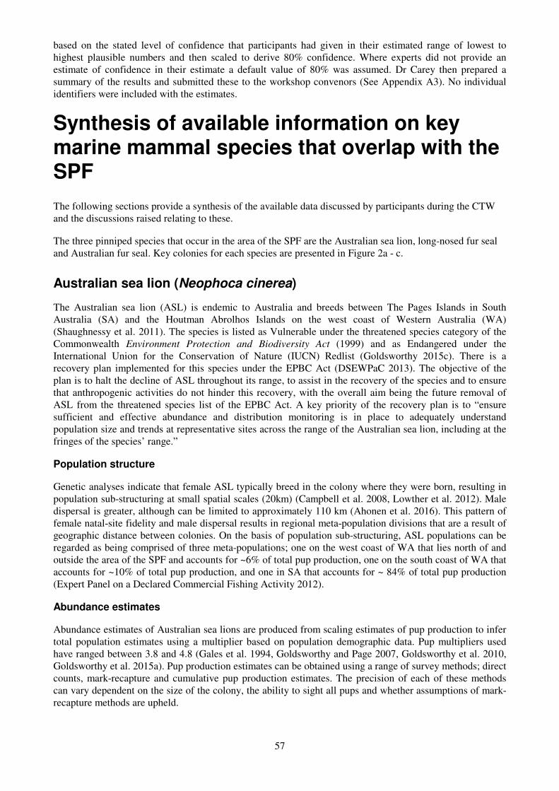
57
based on the stated level of confidence that participants had given in their estimated range of lowest to highest plausible numbers and then scaled to derive 80% confidence. Where experts did not provide an estimate of confidence in their estimate a default value of 80% was assumed. Dr Carey then prepared a summary of the results and submitted these to the workshop convenors (See Appendix A3). No individual identifiers were included with the estimates.
Synthesis of available information on key marine mammal species that overlap with the SPF
The following sections provide a synthesis of the available data discussed by participants during the CTW and the discussions raised relating to these.
The three pinniped species that occur in the area of the SPF are the Australian sea lion, long-nosed fur seal and Australian fur seal. Key colonies for each species are presented in Figure 2a - c.
Australian sea lion (Neophoca cinerea)
The Australian sea lion (ASL) is endemic to Australia and breeds between The Pages Islands in South Australia (SA) and the Houtman Abrolhos Islands on the west coast of Western Australia (WA) (Shaughnessy et al. 2011). The species is listed as Vulnerable under the threatened species category of the Commonwealth Environment Protection and Biodiversity Act (1999) and as Endangered under the International Union for the Conservation of Nature (IUCN) Redlist (Goldsworthy 2015c). There is a recovery plan implemented for this species under the EPBC Act (DSEWPaC 2013). The objective of the plan is to halt the decline of ASL throughout its range, to assist in the recovery of the species and to ensure that anthropogenic activities do not hinder this recovery, with the overall aim being the future removal of ASL from the threatened species list of the EPBC Act. A key priority of the recovery plan is to “ensure sufficient and effective abundance and distribution monitoring is in place to adequately understand population size and trends at representative sites across the range of the Australian sea lion, including at the fringes of the species’ range.”
Population structure
Genetic analyses indicate that female ASL typically breed in the colony where they were born, resulting in population sub-structuring at small spatial scales (20km) (Campbell et al. 2008, Lowther et al. 2012). Male dispersal is greater, although can be limited to approximately 110 km (Ahonen et al. 2016). This pattern of female natal-site fidelity and male dispersal results in regional meta-population divisions that are a result of geographic distance between colonies. On the basis of population sub-structuring, ASL populations can be regarded as being comprised of three meta-populations; one on the west coast of WA that lies north of and outside the area of the SPF and accounts for ~6% of total pup production, one on the south coast of WA that accounts for ~10% of total pup production, and one in SA that accounts for ~ 84% of total pup production (Expert Panel on a Declared Commercial Fishing Activity 2012).
Abundance estimates
Abundance estimates of Australian sea lions are produced from scaling estimates of pup production to infer total population estimates using a multiplier based on population demographic data. Pup multipliers used have ranged between 3.8 and 4.8 (Gales et al. 1994, Goldsworthy and Page 2007, Goldsworthy et al. 2010, Goldsworthy et al. 2015a). Pup production estimates can be obtained using a range of survey methods; direct counts, mark-recapture and cumulative pup production estimates. The precision of each of these methods can vary dependent on the size of the colony, the ability to sight all pups and whether assumptions of mark-recapture methods are upheld.
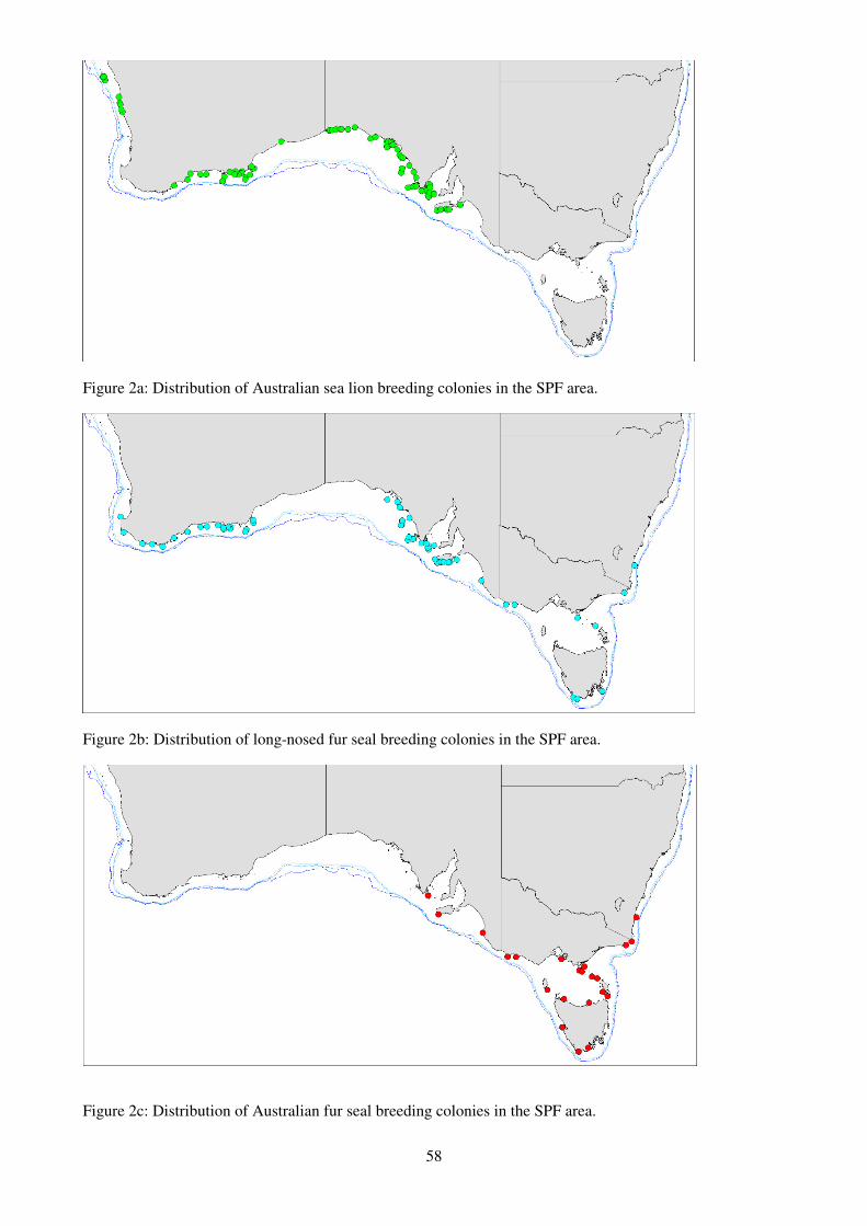
58
Figure 2a: Distribution of Australian sea lion breeding colonies in the SPF area.
Figure 2b: Distribution of long-nosed fur seal breeding colonies in the SPF area.
Figure 2c: Distribution of Australian fur seal breeding colonies in the SPF area.

59
The most comprehensive survey of the ASL population in SA which was conducted in 2014 – 15 (Goldsworthy et al. 2015a), within an 18 month period corresponding to the span of a breeding cycle (Ling and Walker 1978). The total pup abundance was estimated to be 2,520 in 2014/15, with a mean and median pup abundance of 60 (sd = 106.6) and 23, respectively for 42 breeding sites. Only five sites produced more than 100 pups, and these accounted for 58% (1,460) of estimated pup abundance in SA.
When comparing pup abundance in 2014/15 to that derived from equivalent surveys undertaken 6-11 years earlier at a subset of 32 of the breeding sites where data were available, pup abundance declined 23.7% from 2,902 pups to 2,215. Using a multiplier of 3.8 Goldsworthy et al. (2015a) estimated the total size of the ASL population in SA to be 9,652 individuals based on a total pup abundance estimate of 2,520.
There are currently 34 breeding colonies identified in WA. Pup abundance was estimated to be 517 pups (Report of the Expert Panel 2014), with 335 produced in colonies on the southern WA coastline (i.e. within the SPF management areas). Using the 3.8 multiplier, the south coast WA ASL population is estimated to be ~1,270.
The pup multiplier of 3.83 used by Goldsworthy et al. (2015a) is based on ASL survival estimates (Goldsworthy et al. 2010). However, given reductions in pup abundance observed over the last decade, a lower multiplier may be more appropriate (Goldsworthy et al. 2015a).
Published abundance data considered during the CTW are presented in Table 1. Some experts felt that given the reasonably good quality data available on ASL abundance that elicitation should not be undertaken by the group for this species, but instead should be undertaken by one expert who would then record all uncertainties around the estimate.
Table 1: Published estimates of Australian sea lion pup abundance in the area of the Small Pelagic Fishery considered by participants of the Closed Technical Workshop.
Location Year of
survey(s)
Estimated
total pup
numbers
Survey method used Source
Colonies on the southern WA coastline
Between 1988 and 2014
335 Direct counts. Department of Parks and Wildlife, Western Australia ASL database.
42 breeding colonies in South Australia
2013-2015 2,520 Direct count, mark-recapture, cumulative mark-recapture
Goldsworthy et al. (2015a)
Long-nosed fur seal (Arctocephalus forsteri) – formerly New Zealand fur seal
The long-nosed fur seal (LNFS) is listed as a Marine species under the EPBC Act (1999) and globally as of Least Concern under the IUCN Red List. Within Australia, LNFS breed between south-west WA and NSW, with the majority (80%) of the population occurring in SA (Shaughnessy et al. 2015). The species was extensively exploited by sealers in SA between 1800 and 1830, resulting in major reductions in both the range and abundance of the species. Numbers remained at low levels for almost 140 years, after which they began to recover and new colonies were established across their former range (Shaughnessy et al. 2015). Recovery of LNFS since the 1970’s has in part been due to protection of the breeding colonies by State and Commonwealth governments (Shaughnessy et al. 2015).
LNFS feed in shelf waters targeting pelagic and bentho-pelagic prey, and off-shelf waters where they target epipelagic prey (Baylis et al. 2012). Both foraging strategies and diet differ with age and sex (Page et al. 2006). Adult females nursing young initially forage in shelf waters before switching to long foraging trips in

60
oceanic, off-shelf, waters (Baylis et al. 2012). Juvenile and sub-adult males appear to forage predominantly over shelf waters (Page et al. 2006).
Population structure
There is some evidence of population structuring across the breeding range, with genetic variation observed between individuals from SA, Tasmania and New Zealand but little variation observed between individuals from WA and SA (Berry et al. 2012). Movement of a small number of marked individuals between New Zealand and southern Australia has been recorded (Shaughnessy et al. 2001).
Abundance estimates
Abundance estimates of LNFS are produced from scaling estimates of pup production to total population estimates using a multiplier. Pup production estimates can be obtained using a range of survey methods; direct counts and mark-recapture. The precision of each of these methods can vary dependent on the size of the colony and the ability to sight all pups.
LNFS breeding has been recorded at 65 sites across southern Australia, (36 in SA, 20 in WA, four in both Tasmania and Victoria and one in NSW) (Campbell et al. 2014, McIntosh et al. 2014, Shaughnessy et al. 2015). A State-wide survey of LNFS across SA during the 2013/14 breeding season estimated pup abundance to be 20,431, (range 20,312–20,549) representing an estimate 3.6 times greater than that recorded in 1989-90 using similar methods (Shaughnessy et al. 2015). Surveys of 17 breeding sites in WA in 2010-11 estimated a pup abundance of 3,518 from direct counts (Campbell et al. 2014). Pup abundances during the 2013-14 breeding season at four breeding colonies within Victoria, Tasmanian Bass Strait and New South Wales were estimated at 198 ± 13 live pups using mark-recapture and direct counts (McIntosh et al. 2014, DPIPWE unpublished data). These are likely to be underestimates of pup production as surveys occurred before the end of the breeding season and not all breeding sites were surveyed. To estimate total LNFS abundance from pup production estimates, Shaughnessy et al. (2015) used a multiplier of 4.76 developed by Goldsworthy and Page (2007), while Campbell et al. (2014) used multipliers of 4.76 – 4.9 based on two structured population models for LNFS (Shaughnessy et al. 1994, Goldsworthy and Page 2007). Goldsworthy and Page (2007) based their multiplier on life-tables generated from population demographic studies of LNFS at Cape Gantheaume (McKenzie, 2006).
While the overall trend in LNFS populations is increasing, the rate of population growth varies among colonies across the range of the species. Two breeding sites on Kangaroo Island have increased by 15.3% and 19.1% over 12-13 breeding seasons, while those at the Neptune and Liguanea Islands (which account for 47.5% of pup production in SA) appear to have reached carrying capacity (Shaughnessy et al. 2014). Between 1989 and 1999, the annual growth rate of LNFS pup production in WA was estimated to be 10% per annum. Growth rates over the following 12 years were estimated at approximately 1% per annum, indicating colonies in WA may have also reached carrying capacity (Campbell et al. 2014). Pup production increased by 8% between 2008 and 2014 when counts from Victoria, Tasmanian Bass Strait and NSW were combined (McIntosh et al. 2014).
However, pup production at colonies in Bass Strait shows minimal growth, while pup numbers are increasing at Montague Island, NSW. Using a multiplier of 4.70, Shaughnessy et al. (2015) estimated the South Australian population of LNFS to be 97,200 based on 2013/14 pup production estimates. Based on an estimated National pup production of 24,601 and the 4.70 multiplier (Shaughnessy et al. 2015), the total population size is estimated to be ~115,600. Published abundance data considered during the CTW are presented in Table 2.

61
Table 2: Published estimates of long-nosed fur seal pup abundance in the area of the Small Pelagic Fishery considered by participants of the Closed Technical Workshop.
Location Year of
survey(s)
Total pup
numbers
Survey Method
used
Source
17 breeding colonies in
Western Australia
2010/11
breeding season
3,518 Counts Campbell et al.
(2014)
29 breeding colonies in South
Australia
2013 / 14
breeding season
20,431,
(20,312–
20,549)
Counts, mark-
recapture
Shaughnessy et
al. (2015)
Four breeding sites within Vic,
Tasmanian Bass Strait and
NSW
2013/14
breeding season
198 ± 13 Counts and
mark recapture.
McIntosh et al.
(2014)
Australian fur seal (Arctocephalus pusillus doriferus)
Australian fur seals (AUFS) are endemic to southeastern Australia with breeding colonies predominantly located on Victorian and Tasmanian islands in Bass Strait (Kirkwood et al. 2010). Recent surveys indicate an increase in breeding range, with new colonies identified in NSW, western Victoria and Tasmania, and South Australia, as well as an increase in pup numbers at a previously identified colony in South Australia (McIntosh et al. 2014, Shaughnessy et al. 2015). The AUFS is listed as a Marine species under the EPBC
Act (1999) and globally as least concern under the IUCN Red List (2015).
Population structure
The AUFS population is considered to be one single genetic population with high gene flow between colonies maintained by both sexes (Lancaster et al. 2010). AUFS forage almost exclusively on the sea floor, rarely leave the continental shelf, and females typically show strong site fidelity to foraging hotspots (Arnould and Kirkwood 2008, Kirkwood and Arnould 2011). AUFS regularly haul out at a number of sites from the western Eyre Peninsula in SA to Montague Island in NSW (Kirkwood et al. 2010, McIntosh et al. 2014, Shaughnessy et al. 2014). In the last 10 years, new breeding colonies have been established in SA and NSW and in Tasmanian Bass Strait (Kirkwood et al. 2010, McIntosh et al. 2014, Shaughnessy et al. 2014). The group considered that non-breeding adult AUFS that haul out in SA are likely individuals that breed at colonies in the Bass Strait.
Abundance estimates
Abundance estimates of AUFS are produced from estimates of pup production that are then scaled to total population estimates using a multiplier, currently estimated as 4.5 (Gibbens and Arnould, 2009). Since the 2002-2003 breeding season, population estimates of AUFS include a uniform pre-count mortality rate of 15% that is applied to count data. Pup production estimates have been obtained using a range of survey methods: aerial surveys, direct counts and mark-recapture surveys (Kirkwood et al. 2010, McIntosh et al. 2014). AUFS were heavily exploited by sealers between 1798 and 1840. Prior to 2002, AUFS bred at 9 colonies. This increased to 13 established colonies in 2007-2008 and 17 breeding colonies in 2013-14 (McIntosh et al. 2014).
Pup production surveys of breeding sites in Victoria and New South Wales have been undertaken at approximately five-yearly intervals since 2002–03 (Kirkwood et al. 2005, 2010, McIntosh et al. 2014). Estimated pup production from 17 established breeding colonies was 19,820 in 2002-03, 21,881 in 2007–08 and 15,063 in 2013–14 (Kirkwood et al. 2005, 2010, McIntosh et al. 2014). It is unclear if the estimated mean annual 6% decline in pup numbers between the two most recent surveys is indicative of a real decline in the population or is due to high inter annual variability in pup production (McIntosh et al. 2014). Four
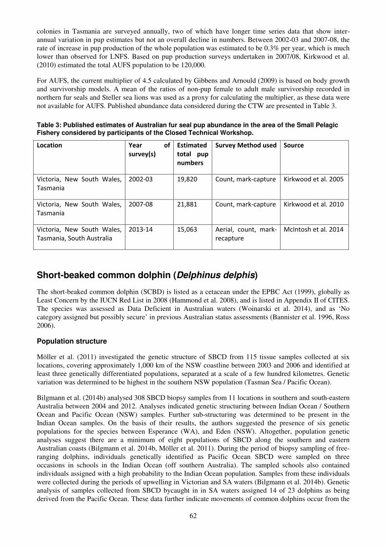
62
colonies in Tasmania are surveyed annually, two of which have longer time series data that show inter-annual variation in pup estimates but not an overall decline in numbers. Between 2002-03 and 2007-08, the rate of increase in pup production of the whole population was estimated to be 0.3% per year, which is much lower than observed for LNFS. Based on pup production surveys undertaken in 2007/08, Kirkwood et al. (2010) estimated the total AUFS population to be 120,000.
For AUFS, the current multiplier of 4.5 calculated by Gibbens and Arnould (2009) is based on body growth and survivorship models. A mean of the ratios of non-pup female to adult male survivorship recorded in northern fur seals and Steller sea lions was used as a proxy for calculating the multiplier, as these data were not available for AUFS. Published abundance data considered during the CTW are presented in Table 3.
Table 3: Published estimates of Australian fur seal pup abundance in the area of the Small Pelagic Fishery considered by participants of the Closed Technical Workshop.
Location Year of
survey(s)
Estimated
total pup
numbers
Survey Method used Source
Victoria, New South Wales,
Tasmania
2002-03 19,820 Count, mark-capture Kirkwood et al. 2005
Victoria, New South Wales,
Tasmania
2007-08 21,881 Count, mark-capture Kirkwood et al. 2010
Victoria, New South Wales,
Tasmania, South Australia
2013-14 15,063 Aerial, count, mark-
recapture
McIntosh et al. 2014
Short-beaked common dolphin (Delphinus delphis)
The short-beaked common dolphin (SCBD) is listed as a cetacean under the EPBC Act (1999), globally as Least Concern by the IUCN Red List in 2008 (Hammond et al. 2008), and is listed in Appendix II of CITES. The species was assessed as Data Deficient in Australian waters (Woinarski et al. 2014), and as ‘No category assigned but possibly secure’ in previous Australian status assessments (Bannister et al. 1996, Ross 2006).
Population structure
Möller et al. (2011) investigated the genetic structure of SBCD from 115 tissue samples collected at six locations, covering approximately 1,000 km of the NSW coastline between 2003 and 2006 and identified at least three genetically differentiated populations, separated at a scale of a few hundred kilometres. Genetic variation was determined to be highest in the southern NSW population (Tasman Sea / Pacific Ocean).
Bilgmann et al. (2014b) analysed 308 SBCD biopsy samples from 11 locations in southern and south-eastern Australia between 2004 and 2012. Analyses indicated genetic structuring between Indian Ocean / Southern Ocean and Pacific Ocean (NSW) samples. Further sub-structuring was determined to be present in the Indian Ocean samples. On the basis of their results, the authors suggested the presence of six genetic populations for the species between Esperance (WA), and Eden (NSW). Altogether, population genetic analyses suggest there are a minimum of eight populations of SBCD along the southern and eastern Australian coasts (Bilgmann et al. 2014b, Möller et al. 2011). During the period of biopsy sampling of free-ranging dolphins, individuals genetically identified as Pacific Ocean SBCD were sampled on three occasions in schools in the Indian Ocean (off southern Australia). The sampled schools also contained individuals assigned with a high probability to the Indian Ocean population. Samples from these individuals were collected during the periods of upwelling in Victorian and SA waters (Bilgmann et al. 2014b). Genetic analysis of samples collected from SBCD bycaught in in SA waters assigned 14 of 23 dolphins as being derived from the Pacific Ocean. These data further indicate movements of common dolphins occur from the
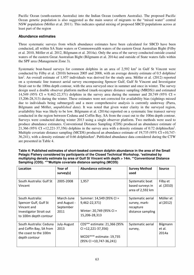
63
Pacific Ocean (south-eastern Australia) into the Indian Ocean (southern Australia). The proposed Pacific Ocean genetic population is also suggested as the main source of migrants to the “mixed water” central NSW population (Möller et al. 2011). This indicates spatial mixing of proposed SBCD populations across at least part of the region
Abundance estimates
Three systematic surveys from which abundance estimates have been calculated for SBCD have been conducted, all within SA State waters or Commonwealth waters of the eastern Great Australian Bight (Filby et al. 2010, Möller et al. 2012, Bilgmann et al. 2014a). Only the area of the survey conducted outside coastal waters of the eastern Great Australian Bight (Bilgmann et al. 2014a) and outside of State waters falls within the SPF area (Management Zone 3).
Systematic boat-based surveys for common dolphins in an area of 2,592 km2 in Gulf St Vincent were conducted by Filby et al. (2010) between 2005 and 2008, with an average density estimate of 0.5 dolphins/ km2. An overall estimate of 1,957 individuals was derived for the study area. Möller et al. (2012) reported on a systematic line transect aerial survey encompassing Spencer Gulf, Gulf St Vincent and Investigator Strait out to the 100m depth contour, with the area surveyed once in summer and once in winter. The survey design used a double observer platform method (mark-recapture distance sampling (MRDS)) and estimated 14,549 (95% CI = 9,462-22,371) dolphins in the survey area during the summer and 20,749 (95% CI = 15,206-28,313) during the winter. These estimates were not corrected for availability bias (sightings missed due to individuals being submerged) and a more comprehensive analysis is currently underway (Parra, Bilgmann and Möller, unpublished data). It was noted that given water clarity in the surveyed region, availability bias was likely to be low. Bilgmann et al. (2014a) reported on a systematic line transect survey conducted in the region between Ceduna and Coffin Bay, SA from the coast out to the 100m depth contour. Surveys were conducted during winter 2013 using a single observer platform. Two methods were used to produce abundance estimates. Conventional Distance Sampling (CDS) produced an abundance estimate of 21,366 (95% CI =12,221-37,356) dolphins in the survey area with a density estimate of 0.72 dolphins/km2. Multiple covariate distance sampling (MCDS) produced an abundance estimate of 19,735 (95% CI =10,747-36,241), with a density estimate of 0.66 dolphin/km2. Published abundance data considered during the CTW are presented in Table 4.
Table 4: Published estimates of short-beaked common dolphin abundance in the area of the Small Pelagic Fishery considered by participants of the Closed Technical Workshop. *estimated by multiplying density estimate by area of Gulf St Vincent with depth > 14m. **Conventional Distance Sampling (CDS). ***Multiple covariate distance sampling (MCDS)
Location Year of
survey(s)
Abundance estimate Survey Method
used
Source
South Australia: Gulf St
Vincent
2005-2008 1,957 Systematic boat
based surveys in
area of 2,592 km
Filby et
al. (2010)
South Australia:
Spencer Gulf, Gulf St
Vincent and
Investigator Strait out
to 100m depth contour
March-June
and August -
September
2011
Summer: 14,549 (95% CI =
9,462-22,371)
Winter: 20,749 (95% CI =
15,206-28,313
Systematic aerial
survey, mark-
recapture
distance sampling
Möller et
al (2012)
South Australia: Ceduna
and Coffin Bay, SA from
the coast to the 100m
depth contour
July-August
2013
CDS** estimate: 21,366 (95%
CI =12,221-37,356)
MCDS*** estimate: 19,735
(95% CI =10,747-36,241)
Systematic aerial
survey,
Bilgmann
et al.
2014a
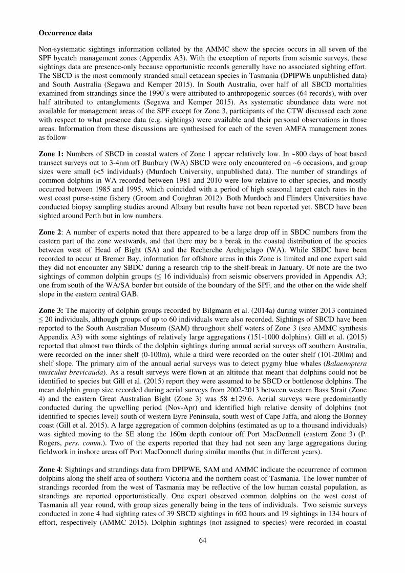
64
Occurrence data
Non-systematic sightings information collated by the AMMC show the species occurs in all seven of the SPF bycatch management zones (Appendix A3). With the exception of reports from seismic surveys, these sightings data are presence-only because opportunistic records generally have no associated sighting effort. The SBCD is the most commonly stranded small cetacean species in Tasmania (DPIPWE unpublished data) and South Australia (Segawa and Kemper 2015). In South Australia, over half of all SBCD mortalities examined from strandings since the 1990’s were attributed to anthropogenic sources (64 records), with over half attributed to entanglements (Segawa and Kemper 2015). As systematic abundance data were not available for management areas of the SPF except for Zone 3, participants of the CTW discussed each zone with respect to what presence data (e.g. sightings) were available and their personal observations in those areas. Information from these discussions are synthesised for each of the seven AMFA management zones as follow
Zone 1: Numbers of SBCD in coastal waters of Zone 1 appear relatively low. In ~800 days of boat based transect surveys out to 3-4nm off Bunbury (WA) SBCD were only encountered on ~6 occasions, and group sizes were small (<5 individuals) (Murdoch University, unpublished data). The number of strandings of common dolphins in WA recorded between 1981 and 2010 were low relative to other species, and mostly occurred between 1985 and 1995, which coincided with a period of high seasonal target catch rates in the west coast purse-seine fishery (Groom and Coughran 2012). Both Murdoch and Flinders Universities have conducted biopsy sampling studies around Albany but results have not been reported yet. SBCD have been sighted around Perth but in low numbers.
Zone 2: A number of experts noted that there appeared to be a large drop off in SBDC numbers from the eastern part of the zone westwards, and that there may be a break in the coastal distribution of the species between west of Head of Bight (SA) and the Recherche Archipelago (WA). While SBDC have been recorded to occur at Bremer Bay, information for offshore areas in this Zone is limited and one expert said they did not encounter any SBDC during a research trip to the shelf-break in January. Of note are the two sightings of common dolphin groups (≤ 16 individuals) from seismic observers provided in Appendix A3; one from south of the WA/SA border but outside of the boundary of the SPF, and the other on the wide shelf slope in the eastern central GAB.
Zone 3: The majority of dolphin groups recorded by Bilgmann et al. (2014a) during winter 2013 contained ≤ 20 individuals, although groups of up to 60 individuals were also recorded. Sightings of SBCD have been reported to the South Australian Museum (SAM) throughout shelf waters of Zone 3 (see AMMC synthesis Appendix A3) with some sightings of relatively large aggregations (151-1000 dolphins). Gill et al. (2015) reported that almost two thirds of the dolphin sightings during annual aerial surveys off southern Australia, were recorded on the inner shelf (0-100m), while a third were recorded on the outer shelf (101-200m) and shelf slope. The primary aim of the annual aerial surveys was to detect pygmy blue whales (Balaenoptera
musculus brevicauda). As a result surveys were flown at an altitude that meant that dolphins could not be identified to species but Gill et al. (2015) report they were assumed to be SBCD or bottlenose dolphins. The mean dolphin group size recorded during aerial surveys from 2002-2013 between western Bass Strait (Zone 4) and the eastern Great Australian Bight (Zone 3) was 58 ±129.6. Aerial surveys were predominantly conducted during the upwelling period (Nov-Apr) and identified high relative density of dolphins (not identified to species level) south of western Eyre Peninsula, south west of Cape Jaffa, and along the Bonney coast (Gill et al. 2015). A large aggregation of common dolphins (estimated as up to a thousand individuals) was sighted moving to the SE along the 160m depth contour off Port MacDonnell (eastern Zone 3) (P. Rogers, pers. comm.). Two of the experts reported that they had not seen any large aggregations during fieldwork in inshore areas off Port MacDonnell during similar months (but in different years).
Zone 4: Sightings and strandings data from DPIPWE, SAM and AMMC indicate the occurrence of common dolphins along the shelf area of southern Victoria and the northern coast of Tasmania. The lower number of strandings recorded from the west of Tasmania may be reflective of the low human coastal population, as strandings are reported opportunistically. One expert observed common dolphins on the west coast of Tasmania all year round, with group sizes generally being in the tens of individuals. Two seismic surveys conducted in zone 4 had sighting rates of 39 SBCD sightings in 602 hours and 19 sightings in 134 hours of effort, respectively (AMMC 2015). Dolphin sightings (not assigned to species) were recorded in coastal
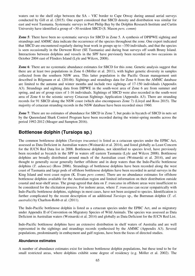
65
waters out to the shelf edge between the SA – VIC border to Cape Otway during annual aerial surveys conducted by Gill et al. (2015). One expert considered that SBCD density and distribution was similar for east and west Tasmania. Systematic surveys in Port Philip Bay by the Dolphin Research Institute and Curtin University have identified a group of ~30 resident SBCD (S. Mason pers. comm)
Zone 5: There have been no systematic surveys for SBCD in Zone 5. A synthesis of DPIPWE sighting and strandings and AMMC data indicate the occurrence of the species throughout the zone. One expert indicated that SBCD are encountered regularly during boat work in groups up to ~350 individuals, and that the species is seen occasionally in the Derwent River (SE Tasmania) and during boat surveys off south Bruny Island. Interactions between dolphins and vessels in the SPF have previously been recorded on two occasions in October 2004 east of Flinders Island (Lyle and Wilcox, 2008).
Zone 6: There are no systematic abundance estimates for SBCD for this zone. Genetic analysis suggest that there are at least two populations in Zone 6 (Möller et al. 2011), with higher genetic diversity in samples collected from the southern NSW area. This latter population is the Pacific Ocean management unit described in Bilgmann et al. (2014b). Sightings and strandings data for Zone 6 from the AMMC database are limited to the autumn and winter months and include two sightings of 17-150 individuals (Appendix A3). Strandings and sighting data from DIPWE in the south-west area of Zone 6 are from summer and spring, and are of group sizes of 1-16 individuals. Sightings of SBCD were also recorded in the south-west area of Zone 6 to the seismic survey Cetacean Sightings Application (Appendix A3). There are stranding records for 91 SBCD along the NSW coast (which also encompasses Zone 7) (Lloyd and Ross 2015). The majority of cetacean stranding records in the NSW database have been recorded since 1960.
Zone 7: There are no estimates of abundance for SBCD in Zone 7, but peaks in bycatch of SBCD in nets set by the Queensland Shark Control Program have been recorded during the winter-spring months across the period 1992-2012 (Meager and Sumpton 2016).
Bottlenose dolphin (Tursiops sp.)
The common bottlenose dolphin (Tursiops trucantus) is listed as a cetacean species under the EPBC Act, assessed as Data Deficient in Australian waters (Woinarski et al. 2014), and listed globally as Least Concern for the IUCN Red Data list in 2008. Bottlenose dolphins, not identified to species level, have previously been recorded as bycatch in the SPF in waters off eastern Tasmania (Lyle and Wilcox 2008). Bottlenose dolphins are broadly distributed around much of the Australian coast (Woinarski et al. 2014), and are thought to generally occur generally further offshore and in deep waters than the Indo-Pacific bottlenose dolphins (T. aduncus) (Ross 2006). Strandings of bottlenose dolphins have been recorded along the west coast of Tasmania and large pods of offshore bottlenose dolphins have been recorded in aerial surveys in the King Island and west coast region (K. Evans pers comm). There are no abundance estimates for offshore bottlenose dolphins available for the Australian region and limited information on their distribution outside coastal and near-shelf areas. The group agreed that data on T. truncatus in offshore areas were insufficient to be considered for the elicitation process. For inshore areas, where T. truncatus can occur sympatrically with Indo-Pacific bottlenose dolphins, sightings in most cases, have not been assigned to species. Identification is further complicated by the recent description of an additional Tursiops sp., the Burrunan dolphin (T. cf. australis) by Charlton-Robb et al. (2011).
The Indo-Pacific bottlenose dolphin is listed as a cetacean species under the EPBC Act, and as migratory under Appendix II of Convention on Migratory Species of Wild Animals. The species was assessed as Data Deficient in Australian waters (Woinarski et al. 2014) and globally as Data Deficient for the IUCN Red List.
Indo-Pacific bottlenose dolphins have an extensive distribution in shelf waters of Australia and are well represented in the sightings and strandings records synthesised by the AMMC (Appendix A3). Several populations, predominantly in embayment and gulf regions, have been the focus of directed studies.
Abundance estimates
A number of abundance estimates exist for inshore bottlenose dolphin populations, but these tend to be for small restricted areas, where dolphins exhibit some degree of residency (e.g. Möller et al. 2002). The

66
assessment of abundance for the southern Australian region is complicated by the unresolved taxonomy of the Tursiops genus, with two species described from inshore waters, the Indo-Pacific bottlenose dolphin T.
aduncus and the Burrunan dolphin, T. australis (Charlton-Robb et al. 2011). Given the distribution of inshore bottlenose dolphins, available spatial information was largely restricted to coastal regions (i.e. State waters), including gulfs and embayments. Therefore, while the species may not directly overlap with fishing operations in the SPF, bycatch of Tursiops sp. have been recorded in other Commonwealth managed fisheries (AFMA 2014b), so it was included in the elicitation process to allow synthesis of current information on its abundance and distribution. It was also noted that there appears to be an offshore gradient in the density of inshore bottlenose dolphins with lower numbers further offshore, and a number of participants commented that densities may be higher in areas like estuaries compared to open coastal areas.
Zone 1: One expert noted that based on preliminary genetic data, there may be more than one species of inshore Tursiops in Zone 1. Robust abundance estimates of bottlenose dolphins are available from Bunbury, WA (Smith et al. 2013) and the Swan River (Chabanne et al. 2012).
Zone 2: Experts noted that there may be a lack of continuity in the coastal distribution of the species in the region between west of Head of Bight (SA) and the Recherche Archipelago (WA), based on observations during flights in the region (S. Goldsworthy pers comm). There are currently no abundance estimates for coastal Tursiops sp. for this zone.
Zone 3: Published abundance estimates for coastal Tursiops spp. were limited to the Port Adelaide River and Barker Inlet estuary (Cribb et al. 2013). Aerial survey data are available for the Spencer Gulf and Gulf St Vincent; analyses are not complete, but preliminary estimates suggest that combined abundance for both gulfs may be approximately 3000 individuals (Flinders University unpublished data). Unpublished data from an early aerial survey estimate in Spencer Gulf in April was of at least a thousand individuals (C. Kemper pers comm). Genetic analysis of 84 biopsy suggest that bottlenose dolphins sampled in the Spencer Gulf are genetically differentiated to those sampled west of the gulf at Flinders Island and Coffin Bay (Bilgmann et al. 2007). Analysis of population structure with a larger sample and additional sampling sites including southern WA, Gulf St Vincent, and Cape Jervis is currently underway at Flinders University.
Zone 4: Stranded bottlenose dolphins in Tasmania have been confirmed to be T. truncatus using molecular and morphological data. There is no confirmation in the DPIPWE stranding dataset of T. aduncus. Molecular analyses indicated that strandings in the northern Bass Strait may also include T. australis, but identification of species and their distribution is preliminary (K. Evans pers comm). Mark-recapture studies of a resident population of bottlenose dolphins in Port Philip Bay have estimated an abundance of 80-100 individuals (reviewed in Woinarski 2014). There is currently little information on the distribution and abundance of bottlenose dolphins in waters west of Port Philip Bay.
Zone 5: There are no published abundance estimates for coastal bottlenose dolphins in Zone 5. Information on inshore bottlenose dolphins is limited by a lack of discrimination between Tursiops species in available records. Molecular analyses of samples from northern and eastern Tasmania identified both T. truncatus and T. australis in Tasmanian waters (Möller et al. 2008, Charlton-Robb et al. 2011).
Zone 6: Resident populations of inshore bottlenose dolphins have been identified in estuary or embayment areas within Zone 6. A resident population of ~50-150 T. australis was estimated within the estuary area of the Gippsland Lakes (Charlton-Robb et al. 2014). Published estimates of resident T. aduncus are 143-160 in Port Stephens and 63-108 in Jervis Bay (Möller et al. 2002).
Zone 7: Abundance of inshore bottlenose dolphins for the Ballina coastal region was estimated at ~860 individuals, with smaller abundance estimates in the Richmond Rivers and Clarence Rivers estimated at 34 and 71 individuals respectively (reviewed in Woinarski et al. 2014).
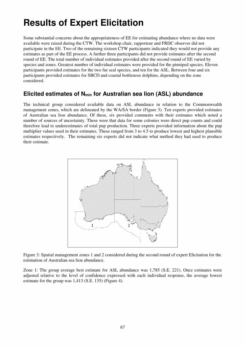
67
Results of Expert Elicitation
Some substantial concerns about the appropriateness of EE for estimating abundance where no data were available were raised during the CTW. The workshop chair, rapporteur and FRDC observer did not participate in the EE. Two of the remaining sixteen CTW participants indicated they would not provide any estimates as part of the EE process. A further three participants did not provide estimates after the second round of EE. The total number of individual estimates provided after the second round of EE varied by species and zones. Greatest number of individual estimates were provided for the pinniped species. Eleven participants provided estimates for the two fur seal species, and ten for the ASL. Between four and six participants provided estimates for SBCD and coastal bottlenose dolphins, depending on the zone considered.
Elicited estimates of Nmin for Australian sea lion (ASL) abundance
The technical group considered available data on ASL abundance in relation to the Commonwealth management zones, which are delineated by the WA/SA border (Figure 3). Ten experts provided estimates of Australian sea lion abundance. Of these, six provided comments with their estimates which noted a number of sources of uncertainty. These were that data for some colonies were direct pup counts and could therefore lead to underestimates of total pup production. Three experts provided information about the pup multiplier values used in their estimates. These ranged from 3 to 4.5 to produce lowest and highest plausible estimates respectively. The remaining six experts did not indicate what method they had used to produce their estimate.
Figure 3: Spatial management zones 1 and 2 considered during the second round of expert Elicitation for the estimation of Australian sea lion abundance.
Zone 1: The group average best estimate for ASL abundance was 1,785 (S.E. 221). Once estimates were adjusted relative to the level of confidence expressed with each individual response, the average lowest estimate for the group was 1,413 (S.E. 135) (Figure 4).

68
Figure 4: Individual expert and group best estimates of Australian sea lion abundance for Zone 1 from the second round of expert elicitation. Bars represent estimates of lowest and highest plausible estimates of abundance adjusted to the confidence levels experts provided with their estimates.
Zone 2: The group average best estimate was 10,556 (S.E. 642). Once estimates were adjusted relative to the level of confidence expressed with each individual response, the average lowest estimate for the group was 9,378 (S.E. 554) (Figure 5). Three experts provided pup multiplier values used in their estimates. Pup multipliers used to produce lowest estimates ranged from 3 to 3.5, and to produce highest estimates ranged from 3.83 to 4. Given declines in abundance of the species across its range (Goldsworthy et al. 2015a), experts noted that using a multiplier of 3.83, that was developed for a stable population, would likely overestimate total abundance.
Figure 5: Individual expert and group best estimates of Australian sea lion abundance for Zone 2 from the second round of expert elicitation. Bars represent estimates of lowest and highest plausible estimates of abundance adjusted to the confidence levels experts provided with their estimates. Elicited estimates of Nmin for long nosed fur seal abundance

69
Elicited estimates of Nmin for long-nosed fur seal (LNFS) abundance
AFMA currently does not use spatial zones to manage interactions between the SPF and fur seal species. The technical group considered LNFS in relation to three management zones based on distribution of the key breeding colonies for the species (Figure 6).
Figure 6: The three spatial management zones considered during the second round of expert elicitation for the estimation of long-nosed fur seal abundance.
Eleven experts provided estimates of LNFS abundance in the three proposed spatial zones. Five experts provided comments with their estimates noting available pup count data considered for each zone had uncertainty associated with survey methods and the length of time that has passed since the most recently available surveys were undertaken. It was also noted that estimated pup numbers were likely underestimates as total pup mortality across the breeding season was not recorded.
Zone 1: The group average best estimate of LNFS abundance was 16,574 (S.E. 1,201). Once estimates were adjusted relative to the level of confidence expressed with each individual response, the average lowest estimate for the group was 14,379 (S.E. 1,287) (Figure 7). Three experts provided the pup multiplier values used in their estimates. These ranged from 3.5 to 4 to produce lowest plausible estimates, and 4.76 to 5 for the highest plausible estimates of LNFS abundance.

70
Figure 7: Individual expert and group estimates of lowest long-nosed fur seal abundance in Zone 1 from the second round of expert elicitation. Confidence intervals represent derived 80% confidence adjusted from the confidence levels experts provided with their estimates.
Zone 2: The group average best estimate of LNFS abundance was 91,945 (S.E. 7,250). Once estimates were adjusted relative to the level of confidence expressed with each individual response, the average lowest estimate for the group was 83,292 (S.E. 7,685) (Figure 8). Three experts provided the pup multiplier values used in their estimates. These ranged from 3.5 to 4 to produce lowest estimates, and 4.76 to 5 for the highest estimates of LNFS abundance.
Figure 8: Individual expert and group best estimates of long-nosed fur seal abundance in Zone 2 from the second round of expert elicitation. Bars represent estimates of lowest and highest plausible estimates of abundance adjusted to the confidence levels experts provided with their estimates.
Zone 3: The group average best estimate of LNFS abundance was 3,363 (S.E. 279). Once estimates were adjusted relative to the level of confidence expressed with each individual response, the average lowest estimate for the group was 2,708 (S.E. 363) (Figure 9). Three provided the pup multiplier values used in

71
their estimates. These ranged from 3.5 to 4 to produce lowest estimates, and 4.76 to 5 for the highest estimates of LNFS abundance.
Figure 9: Individual expert and group best estimates of long-nosed fur seal abundance in Zone 3 from the second round of expert elicitation. Bars represent estimates of lowest and highest plausible estimates of abundance adjusted to the confidence levels experts provided with their estimates.
Elicited estimates of Nmin for Australian fur seal (AUFS) abundance
The technical group considered AUFS in relation to a single management zone (Figure 10). Eleven experts provided estimates of AUFS abundance for the spatial management zone. Five experts provided comments with their estimates noting lack of annual surveys for the species at some locations, uncertainty associated with pup count precision depending on survey methods, the length of time that has passed since the most recently available surveys were undertaken and estimates of total pup mortality.
Figure 10: Management Zone 1 considered during the second round of expert elicitation for the estimation of Australian fur seal abundance.

72
Zone 1: The group average best estimate of AUFS abundance was 104,259 (S.E. 9,936). Once estimates were adjusted relative to the level of confidence expressed with each individual response, the average lowest estimate for the group was 87,424 (S.E. 10,415) (Figure 11). Two experts provided the pup multiplier values used in their estimates. These ranged from 3.5 to 4.4, and two noted that they had incorporated pup mortality rates of 15%, based on previous AUFS studies, into their estimates.
Figure 11: Individual expert and group best estimates of Australian fur seal abundance in Zone 1 from the second round of expert elicitation. Bars represent estimates of lowest and highest plausible estimates of abundance adjusted to the confidence levels experts provided with their estimates.
Elicited estimates of Nmin for short-beaked common dolphin (SBCD) abundance
The technical group considered SBCD abundance estimates in relation to the seven management zones currently used by AFMA to manage interactions with dolphins in the SPF (Figure 12).
Figure 12: The seven bycatch management zones used by AFMA to manage dolphin interactions within the SPF.
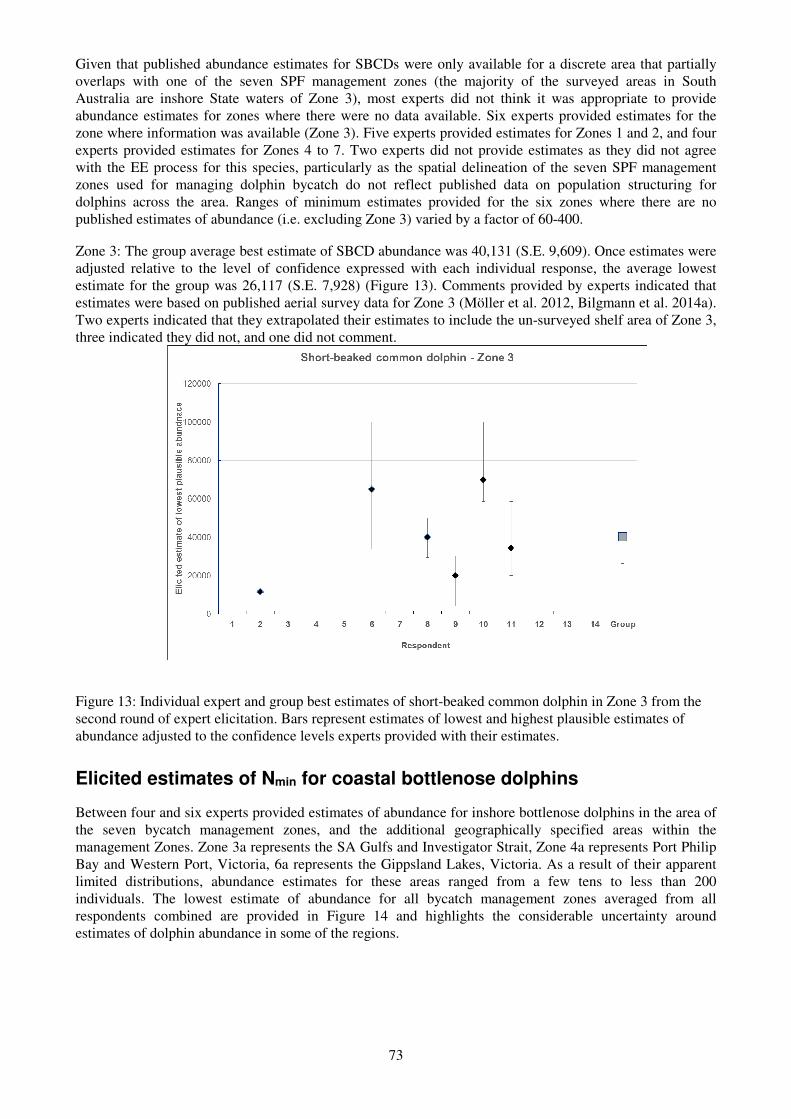
73
Given that published abundance estimates for SBCDs were only available for a discrete area that partially overlaps with one of the seven SPF management zones (the majority of the surveyed areas in South Australia are inshore State waters of Zone 3), most experts did not think it was appropriate to provide abundance estimates for zones where there were no data available. Six experts provided estimates for the zone where information was available (Zone 3). Five experts provided estimates for Zones 1 and 2, and four experts provided estimates for Zones 4 to 7. Two experts did not provide estimates as they did not agree with the EE process for this species, particularly as the spatial delineation of the seven SPF management zones used for managing dolphin bycatch do not reflect published data on population structuring for dolphins across the area. Ranges of minimum estimates provided for the six zones where there are no published estimates of abundance (i.e. excluding Zone 3) varied by a factor of 60-400.
Zone 3: The group average best estimate of SBCD abundance was 40,131 (S.E. 9,609). Once estimates were adjusted relative to the level of confidence expressed with each individual response, the average lowest estimate for the group was 26,117 (S.E. 7,928) (Figure 13). Comments provided by experts indicated that estimates were based on published aerial survey data for Zone 3 (Möller et al. 2012, Bilgmann et al. 2014a). Two experts indicated that they extrapolated their estimates to include the un-surveyed shelf area of Zone 3, three indicated they did not, and one did not comment.
Figure 13: Individual expert and group best estimates of short-beaked common dolphin in Zone 3 from the second round of expert elicitation. Bars represent estimates of lowest and highest plausible estimates of abundance adjusted to the confidence levels experts provided with their estimates.
Elicited estimates of Nmin for coastal bottlenose dolphins
Between four and six experts provided estimates of abundance for inshore bottlenose dolphins in the area of the seven bycatch management zones, and the additional geographically specified areas within the management Zones. Zone 3a represents the SA Gulfs and Investigator Strait, Zone 4a represents Port Philip Bay and Western Port, Victoria, 6a represents the Gippsland Lakes, Victoria. As a result of their apparent limited distributions, abundance estimates for these areas ranged from a few tens to less than 200 individuals. The lowest estimate of abundance for all bycatch management zones averaged from all respondents combined are provided in Figure 14 and highlights the considerable uncertainty around estimates of dolphin abundance in some of the regions.

74
Figure 14: Average group best estimates for inshore bottlenose dolphin abundance across all bycatch management zones and subregions during the second round of expert elicitation. Bars represent average group estimates of lowest and highest plausible estimates of abundance

75
Discussion
The key objective of the CTW was to “review current information available to inform the establishment of trigger limits using PBR for key marine mammal species (especially the short-beaked common dolphin, and Australian and long-nosed fur seals)”. Structured expert elicitation was chosen as a method to synthesise available data on key marine mammal species, integrate expert knowledge and, if possible, to elicit estimates of abundance based on existing data that could then be used to calculate PBR.
The CTW was successful at providing a synthesis of the current available information on the abundance, distribution and ecology of Australian sea lions, Australian and long-nosed fur seals, short-beaked common dolphins and inshore bottlenose dolphins. Workshop discussions focused on factors affecting the precision of existing abundance estimates and highlighted data gaps for each species.
However, participants of the CTW raised a number of concerns about the EE process. The key concern was that while EE can provide a means of synthesising expert judgment, it should not be used as a method to obtain “estimates” of abundance in the absence of empirical data. There was also concern that estimates not based on empirical data would be used to calculate PBR. Two participants of the CTW stated they would not provide estimates during the EE process, and a further three did not provide estimates after the second round of EE. Therefore, there is a disparity between the numbers of participants who attended the closed technical workshop and the number of estimates provided across species and areas.
Additional concerns which participants raised during the CTW about the EE process were:
• The short timeframe given to complete the first elicitation process.
• Lack of clarity during the first elicitation with respect to current AFMA management zones in the
SPF and how these related to management of the three pinniped species.
• The appropriateness of the seven zones used to manage dolphin interactions in the SPF given
published studies of short-beaked common dolphin and bottlenose dolphin species population
structuring (e.g. Möller et al. 2011, Bilgmann et al. 2014b).
Estimates of abundance from expert elicitation
The greatest number of estimates provided by participants during the EE process were for the three pinniped species. The high level of participation reflects the availability of published information on abundance estimates for these species across their ranges. The average minimum group EE estimates for the three pinniped species generally reflected published estimates. For all species, comments provided highlighted uncertainties surrounding precision in estimating pup abundance, estimation of pup mortality, and the appropriate multiplier value to use to scale pup numbers to total abundance estimates.
The two management Zones used by AFMA under the Australian sea lion strategy reflect a natural break at the SA / WA border in the distribution of ASL colonies. Ten participants provided estimates of ASL abundance in each zone. After adjustment to the level of confidence expressed with each individual response, the average minimum group EE estimates of abundance from ten respondents was were similar to published estimates of abundance for ASL. For Zone 1 the EE minimum estimate of abundance was 1,413 (S.E. 135) compared to the most recent published abundance estimates of 1,270 individuals (Report of the Expert Panel 2014). Comments noted that the most recent surveys undertaken in Zone 1 have been between 1988 and 2014 and therefore there is uncertainty surrounding the current pup estimate of 335 for the Zone. There is a need for a more comprehensive survey of ASL colonies in WA to reduce uncertainty in abundance estimates. For Zone 2 the EE estimate of abundance was 9,378 (S.E. 554) compared to results of a comprehensive state wide survey of all colonies in SA that produced an abundance estimate of 9,652 (Goldsworthy et al. 2015a). For Zone 2, two responders estimated minimum plausible numbers at 12,747 and 11,000, but did not provide comments on how they had produced these estimates. Six responders provided comments noting that key main uncertainty in abundance estimates was the choice of what pup multiplier value to use, given that the multiplier of 3.8 used by Goldsworthy et al. (2015a) is based on a stable population.

76
As AFMA do not use spatial zones to manage interactions with fur seals, the CTW agreed that elicited estimates of LNFS would consider three zones that reflected the distribution of colonies for this species. Eleven participants provided estimates of LNFS abundance in each zone After adjustment to the level of confidence expressed with each individual response, the average minimum group EE estimates for LNFS in Zone 1 (WA) was 14,379 (S.E. 1,287). The most recent abundance estimate for LNFS in WA is 17,200 based on a total pup counts of 3,518 in 2010/11 (Campbell et al. 2014). For Zone 2 (SA), after adjustment to the level of confidence expressed with each individual response, the average minimum group EE estimates was 83,292 (S.E. 7,685). This compares to a recent abundance estimate of 97,200 in 2013/14 (Shaughnessy et al. 2015). For Zone 3 (VIC, TAS, NSW), after estimates were adjusted to reflect the level of confidence expressed with each individual response, the average minimum group EE estimate was 2,708 (S.E. 362). Most recent pup abundance estimates for this species in Zone 3 was 198 ± 13 live pups using mark-recapture and direct counts (McIntosh et al. 2014, DPIPWE unpublished data).
The CTW considered AUFS estimates for a single zone covering the known distribution that is considered to be one single genetic population with high gene flow between colonies maintained by both sexes. Eleven participants provided estimates, and after adjustment to the level of confidence expressed with each individual response, the average minimum group EE estimates was 87,424 (S.E. 10,415). Based on pup production surveys undertaken in 2007/08, Kirkwood et al. (2010) estimated the total AUFS population to be 120,000. Estimated pup production from 17 established breeding colonies was 19,820 in 2002-03, 21,881 in 2007–08 and 15,063 in 2013–14 (Kirkwood et al. 2005, 2010, McIntosh et al. 2014). The lowest plausible estimate provided by one respondent was 19,000 individuals, but no comments were provided to how they produced this estimate.
The following uncertainties in estimating abundance of pinniped species were discussed during the CTW and mentioned in comments provided with some EE estimates.
The suitability of direct counts to estimate pup production is dependent on how possible it is to sight all pups present and the size of the colony involved. Counts are more reliable for small colonies where pups can easily be found. Mark-recapture techniques and cumulative pup production methods can increase the precision in the abundance estimate. For the two fur seal species, where breeding is synchronous for the entire population and occurs over a discrete period, mark-recapture surveys to estimate pup production can be timed to occur towards the end of the breeding season when all pups are still of an age class that will be on land and available for counting. In contrast, ASL breed asynchronously across their range and the duration of the breeding season varies with the size of the colony. Given this asynchrony, a critical aspect of reducing uncertainty in abundance estimates is timing the survey correctly with respect to the breeding season regardless of the survey method used. The ability to determine the timing of breeding is confounded by inconsistency in the interbreeding interval between colonies, which has been estimated to range from 16 to 19.9 months.
For ASL colonies with extended breeding seasons (6-9 months), where pups born at the beginning of the season can have already moulted while other pups are still being born, surveys are aimed to commence in the third month of the breeding season. For small sites, which have shorter breeding seasons, direct count methods are used at the end of the breeding season, which typically last 3-4 months. For sites where direct counts are not suitable, or for sites where the breeding season is longer, multiple surveys provide better estimates of pup abundance. Cumulative pup production methods provide an estimate of total number of pups that are present at each survey as well as the cumulative number of pups that were produced between surveys. Goldsworthy et al. (2015a) provide a review of appropriate survey methods.
Direct counts of live pups will underestimate the total number of pups produced within a breeding season in a colony as they do not account for pup mortality rates. Counts of dead pups at the end of the breeding season are known to lead to underestimates of pup mortality due to natural decomposition, scavenging by predators and removal by high tides and storms over the 2-3 month pupping period (Shaughnessy and McKeown 2002). LNFS pup mortality from birth to the end of the breeding season has been recorded to range from 9.6 to 22.2% based on observational data over four breeding seasons at Cape Gantheaume (McKenzie 2006). While pup mortality is likely to vary between colonies, comparison of the two methods
suggest pup mortality rates are on average 6.8% ± 1.4 (SD) greater than estimated from counts of dead pups at the end of the breeding season (McKenzie 2006).

77
For AUFS, a historically derived pup mortality rate of 15% (Kirkwood et al. 2010) has been applied to estimate total pup production based on the total number of live pups counted (McIntosh et al. 2014). McIntosh et al. (2014) validated this estimate in the 2013-14 season at Seal Rocks, where they recorded 14% mortality of all pups born. It is unclear whether pup mortality rates are consistent across the species range, particularly at sites that may be expanding or those that are particularly exposed where pups are at risk of being washed from colonies during storm events. Levels of ASL pup mortality fluctuate between breeding seasons at some breeding sites, but seasonal variations in pup mortality are not consistent across sites (McIntosh et al. 2012). At Seal Bay (SA), average ASL pup mortality recorded over six seasons is 28% (range 20.8 - 41.8%) (Goldsworthy et al. 2015b).
Comments provided with estimates for the pinniped species noted the potential choice(s) of multipliers that could be used to estimate total population size. A range of multipliers have been applied to pup counts for AUFS, LNFS and ASL based on species specific life history tables. However, the relationship between pup production and population size can vary dependent on a number of factors such the trend in the population, changes in survival for different age classes and changes in fecundity and / or pupping rates, which can also vary between breeding seasons and between colonies.
Participation in EE for the two cetacean species was lower than for the pinniped species, and ranged from four to six responses by species or zone. The lower participation rate reflects the lack of data on the abundance of SBCD and bottlenose dolphin species for most of the area of the SPF. The CTW considered SBCD and BND abundance estimates in relation to the seven management zones currently used by AFMA to manage interactions with dolphins in the SPF. The CTW noted that the current spatial delineation of the management zones does not reflect the most recently published data on the genetic structure of short-beaked common dolphins in Australian waters (Möller et al. 2011, Bilgmann et al. 2014b). Two participants withdrew from providing estimates for SBCD as they did not agree with either the EE process for this species or the delineation of the seven management zones used by AFMA to manage dolphin interactions.
Six participants provided estimates for SBCD for Zone 3, and four or five provided estimates for all other zones. Abundance estimates for SBCD are only available for part of the area of SPF management Zone 3 in Gulf and shelf waters out to the 100m depth contour (Filby et al. 2010, Möller et al. 2012, Bilgmann et al. 2014a). Published abundance estimates for the South Australian Gulfs and shelf area out to 100m which were 14,549 (CI=9,462-22,371) in summer and 20,749 (CI=15,206-28,313) in winter (Möller et al. 2012). For the eastern Great Australian Bight, estimates between Ceduna and Coffin Bay out to the 100m depth contour were between 19,735 (CI=10,747-36,241) and 21,366 (CI=12,221-37,356) (Bilgmann et al. 2014a). After adjustment to the level of confidence expressed with each individual response, the average minimum group EE estimates of for SBCD in Zone 3 of 26,117 (S.E. 7,928).Therefore the lowest adjusted group estimate was within the summed confidence intervals of the abundance estimates produced by Möller et al (2012) and Bilgmann et al. (2014a). For the other management zones, four to five experts provided estimates. These varied greatly reflecting the fact that there is no information for abundance of SBCD in these zones.
The group noted that there is no information on the abundance of SBCD in off-shelf waters or the level of mixing (either spatially or genetically) between inshore and offshore areas. While the group noted that the seven AFMA management zones do not reflect the most recently published data on the population structure of short-beaked common dolphins in Australian waters (Möller et al. 2011, Bilgmann et al. 2014b), some experts did not feel the population structure of SBCD in Australian waters was fully resolved. Experts also questioned the applicability of spatial management zones for highly mobile marine species noting evidence indicating longitudinal movement of individuals from different populations between SPF management zones (Bilgmann et al. 2014b). A number of experts also raised concerns that two different populations had been identified by Bilgmann et al. (2014b) within the spatial area of Management Zone 3. Managing two populations within a single zone as a single unit will confound interpretation of impacts of anthropogenic mortality if mortality disproportionately affects one population and not the other. This may be a particular issue if anthropogenic mortality occurs at discrete temporal and / or spatial scales.
In contrast to highly mobile dolphin species such as SBCD, inshore bottlenose dolphins are often found to show high residency patterns in discrete geographic areas such as coastal bays and gulfs. Therefore, in addition to the seven management zones in the SPF, the CTW provided abundance estimates for inshore bottlenose dolphin species specifically for the SA gulfs and Investigator Strait, Port Philip Bay and Western

78
Port and the Gippsland lakes. Between four and six participants provided estimates of abundance for inshore bottlenose dolphins. After adjustment to the level of confidence expressed with each individual response, the average minimum group EE estimates of coastal bottlenose dolphins ranged from 111 (S.E. 66) in Zone 6a (Gippsland Lakes) to a maximum of 1,074 (S.E. 591) in Zone 3a (SA gulfs and Investigator Strait). However, the standard error around average group minimum estimates was large for all zones, reflecting wide variability in estimates provided. For example, in Zone 3a where published abundance data is available for a discrete area (Cribb et al. 2013), individual minimum estimates, adjusted to the level of confidence expressed, ranged from 84 to 3,667. Comments provided by experts indicated the lack of formal abundance data for coastal bottlenose dolphin in most zones. Although inshore bottlenose dolphin species are unlikely to overlap with trawl operations in the SPF, the group agreed to consider them in the EE process as they are known to get bycaught in other fisheries (AFMA 2014b). Small populations are inherently more susceptible to extinction due to increased mortalities (anthropogenic or other) than larger populations.
Participants of the CTW agreed not to undertake EE to estimate abundance of bottlenose dolphins in offshore areas, as there are no abundance estimates for offshore bottlenose dolphins available for the Australian region and limited information on their distribution outside coastal and near-shelf areas (Ross 2006).
Abundance estimates for cetaceans are obtained using systematic surveys that use conventional mark-recapture distance-sampling methods and/or using mark-recapture analysis based on photo-ID. Systematic visual boat-based or aerial surveys provide the ability to cover large areas to estimate abundance of cetacean species when the species range is adequately covered. Surveys need to be designed to ensure that survey transect lines provide equal coverage probability of the area and that surveys are conducted across any density gradients that may exist. Biases in the data collected from these surveys exist due to the assumptions that all animals on the transect line will be detected, no animal movement occurs in response to the survey platform, there is no error in measurement of distance from a sighted animal to the survey line, and that the survey lines are laid at random with respect to the distribution of animals (e.g. across, not along density gradients) and are at an adequate spacing to reduce the likelihood of resighting the same individual(s) across the survey area.
The probability of detecting an animal on a survey transect line is estimated from survey data by developing detection functions based on the perpendicular distances to sightings from the transect line. The ability to detect animals during surveys will be affected by the behaviour of a species, as well as environmental factors such as wind and swell. Errors in how distances and angles to sightings are judged can be improved by using a double observer platform method. This approach uses two independent teams of observers to allow for calculation of sightings that might be missed by one team along the transect line. In the case of boat-based surveys, where avoidance of or attraction to boats is observed for some species, the double platform methodology also records the movement responses of animals to the boat. Responsive movement can then by accounted for during analysis of sightings data. If estimates do not account for responsive movement towards or away from a survey vessel, sighting rates will either be positively or negatively biased. It is not possible to account for this using single observer platform. Group size estimates are improved by using double observer methods, or surveys can be conducted in “closing mode”, where the survey line is broken and the group is approached to allow better estimation of group size.
Spatial variability in the sighting rates of SBCD has been recorded in those regions that the species has been surveyed (e.g. Filby et al. 2010, Bilgmann et al. 2014a), suggesting that the density of this species may also vary on greater spatial scales. It would therefore be inappropriate to extrapolate population estimates from an area in which the species has been surveyed to an unsurveyed region. Furthermore, aerial surveys to estimate the abundance of SBCD (Möller et al. 2012, Bilgmann et al. 2014a) were undertaken in known areas of high occurrence for this species. Also, current abundance estimates have been produced in areas where more than one genetic population has been identified, and there may be fluctuations in SBCD abundance in South Australian waters as a result of seasonal movement of SBCD from south-eastern Australian waters (Bilgmann et al. 2014b).
Photo-ID mark-recapture techniques are also commonly used to estimate cetacean abundance. Photos of natural markings are used as “marks” and recapture events occur each time the same individual is subsequently identified. Mark-recapture studies of inshore bottlenose dolphins in Australian waters have

79
shown variation in individual residency patterns and emigration rates at the scale of study area (e.g. Möller et al. 2002, Smith et al. 2013)
Feedback on elicitation method and application of workshop outcomes
Elicited estimates that were based on published data provided a synthesis of expert judgement in combining abundance estimates across the species range, considering what pup multiplier(s) would be appropriate for the pinniped species and apportioning estimates between management zones. In general, the participants of the CTW did not agree that EE was an appropriate method for estimating abundance of marine mammal species in the absence of empirical data.
Participants noted that there are well-established procedures for estimating marine mammal abundance (from line-transect, count, and/or mark-recapture data), which could be applied to many of the species/areas of interest to this report. Three participants declined to participate in the EE process, and a further three did not provide estimates after the second round of elicitation. Participation varied greatly between species and zones and reflected the level of published abundance data available for consideration. Results of the EE process showed greatest levels of participation when abundance data were available (e.g. the pinniped species) and an opposition to providing estimates when no abundance data were available (e.g. the cetacean species) or, for two experts, when the spatial zones were not considered appropriate. Morgan (2014) notes that “Although it may be tempting to view expert elicitation as a low-cost, low-effort alternative to conducting serious research and analysis, it is neither. Rather, expert elicitation should build on and use the best available research and analysis and be undertaken only when, given those, the state of knowledge will remain insufficient to support timely informed assessment and decision making.”
One participant stated that “The normal process of scientific peer review is a transparent way for anyone literate in the techniques (not necessarily an "expert" on individual species) to evaluate abundance estimates derived accordingly, as long as the assumptions and steps are clearly documented; if an estimate passes muster under such review, then it is a defensible scientific basis for management action (e.g. for calculating a trigger limit). In contrast, an estimate derived from EE stands outside the scientific paradigm; it is essentially unreviewable even by experts (one can check whether the EE steps were done well or badly, but not whether the input numbers reflected the real data appropriately).”
The consensus of the group was that in the absence of empirical data, elicited estimates should not be used to inform management. Even for those species, and or zones, where abundance data are available, elicited estimates varied between individuals as shown by the large standard errors around the adjusted group estimates. Some responders noted in their comments that they were providing estimates that were precautionary either in the pup multiplier they used or basing their estimate on the lower bound confidence interval of a published abundance estimate. A particular concern raised at the CTW was the potential that elicited abundance estimates that were not based on empirical data would be used in PBR calculations.
A number of participants questioned if PBR was an appropriate method for calculating limits to anthropogenic mortality in Australian fisheries. Comments noted that PBR is only one element of a legislative management framework in the US, and that legislative framework mandates the collection of robust abundance estimates for use in PBR calculation. The undertaking of PBR analyses was a component of this project as a result of a recommendation of a previous FRDC workshop (Fitzgerald et al. 2015) where PBR was identified as a possible means of estimating sustainable limits to anthropogenic mortality of marine mammal species interacting with the SPF. Calculation of PBR levels presented in the main document, was undertaken by the authors after results of the second round of expert elicitation were provided. Only those elicited estimates that were based on empirical data were used to calculate PBR. Participants noted that EE could have been conducted in relation to some of the other inputs into PBR such as a choice of recovery factor or maximum growth rate, which could be based on available data for proxy populations or species. This was outside of the scope of the current project.
Knowledge gaps identified during the closed technical workshop.
A number of data gaps and research needs were identified during the stakeholder workshop and CTW. These related to information needed to specifically inform the setting of quantitative bycatch reference
80
limits, whilst others related to improving information on population trends and dynamics of marine mammal species to manage interactions and or assess anthropogenic impacts.
The CTW synthesised available information and current knowledge gaps for the marine mammal species considered. A key requirement in managing bycatch of protected species is the ability to measure the performance of management measures. Since 2010, AFMA has managed ASL interactions in Commonwealth fisheries using spatial closures and trigger limits. Despite the implementation of these management measures, a recent state-wide surveys of ASL colonies undertaken in South Australia has identified a continuing decline in population abundance (Goldsworthy et al. 2015a). Given that the age of first reproduction in most adult females is between 6 and 10 years (Goldsworthy et al. 2015b), it is unlikely that any population recovery that may result from bycatch management and mitigation measures introduced by AFMA in the SESSF between 2010 and 2012 (AFMA 2010b), will be detectable for some years. Updated life history tables should be generated from the most recent demographic data from long-term monitoring of the ASL colony at Seal Bay, Kangaroo Island, and an appropriate framework developed to identify when or if population recovery, as a result of bycatch management measures, could be detected under a range of scenarios (e.g. the absence and presence of other sources of mortality). There is also a need to improve abundance estimates for the species in WA, especially off the south coast, and assess trends in abundance.
For the two fur seal species, continued monitoring of key colonies was recommended to maintain data required to detect trends in abundance. For AUFS, which are bycaught in the SET sector of the SESSF (Expert Panel on a Declared Commercial Fishing Activity, 2014), information on the age and sex of bycaught individuals would improve assessments of impacts of mortality for this species. The potential for increasing levels of interactions (operational and ecological) between recovering fur seal populations and commercial fisheries was noted as a key knowledge gap during the stakeholder workshop. Improving information on the spatial distribution and foraging and consumption effort of fur seals under a range of population trajectories is required to allow adaptive management of fishery resources.
The workshop identified that abundance data required to inform management are lacking for most cetacean species in Australian waters. There is currently no information on the abundance or distribution of SBCD outside of a discrete area of South Australian waters out to 100m depth. There are no abundance or distribution data for other cetacean species in offshore / off-shelf areas of the SPF management zone. Systematic surveys (boat based and aerial) required to produce estimates of abundance of cetaceans over large areas, particularly offshore areas, require considerable resources, but such data provide an important reference level to assess the impact of bycatch or other anthropogenic activities (Hammond et al. 2002, 2013).
The appropriateness of current spatial management of interactions between dolphin species and the SPF was queried. The CTW noted that spatial management of interactions between SBCD and Commonwealth and State fisheries requires improved information on movement patterns and population structuring. Möller et al. (2011) and Bilgmann et al. (2014b) identified eight genetic populations of SBCD between Esperance, WA and Eden, NSW. Participants of the CTW noted that further work should be conducted to resolve population structuring for this species, particularly sampling of dolphins in offshore areas across the distribution range. The level of genetic structure described for SBCD in Australian waters (Möller et al. 2011, Bilgmann et al. 2014b) is very different to SBCD in other areas. In the Northeast Atlantic, SBCD ranging from waters off Scotland to Portugal are considered a single panmictic population (ICES 2013, Moura et al. 2013), and in the Northwest Atlantic SBCD are considered a single panmictic population (Waring et al. 2015).
Bilgmann et al. (2014b) proposed that long range longitudinal movements of SBCD occur during periods of upwelling in SA. The use of satellite tagging would provide direct observations of movement (both longitudinal and inshore-offshore) that could be used to assess risks of fisheries interactions of different populations with respect to area and season. Information on temporal and spatial distribution and population structure of SBCD will inform assessment of impacts of anthropogenic mortality and risk of exposure of populations, particularly if large scales seasonal movements are evident. Analysis of archived samples for this species could be used to estimate life history parameters for the species in Australian waters.
Participants of the CTW highlighted the importance of collecting samples from landed bycaught marine mammals where possible to determine sex and age class and population being impacted. A draft discussion document for the development of a framework to collect biological samples from bycaught TEPS was

81
developed during the CTW (Appendix A4). The CTW acknowledged that the collection of these data would require industry participation, particularly with the move to EM in many fisheries. The perceived potential risk associated with the collection of such data, such as increased management measures, may be a barrier to industry participation. It was also noted that for such a biological sampling scheme to work, secured funding and procedures would need to be in place to ensure samples are analysed.
82
References
Adams-Hosking, C., McBride, M. F., Baxter, G., Burgman, M., de Villiers, D., Kavanagh, R., Lawler, I., Lunney, D., Melzer, A., Menkhorst, P., Molsher, R., Moore, B. D., Phalen, D., Rhodes, J. R., Todd, C., Whisson, D. and McAlpine, C. A. (2015). Use of expert knowledge to elicit population trends for the koala (Phascolarctos cinereus). Diversity and Distributions. doi:10.1111/ddi.12400
AFMA (2010a). Ecological Risk Management. Report for the midwater trawl sector of the Small pelagic Fishery http://www.afma.gov.au/wp-content/uploads/2014/11/Ecological-Risk-Management-SPF-midwater-trawl-March-2010.pdf
AFMA (2010b). Australian Sea Lion Management Strategy. Southern and eastern Scalefish and Shark Fishery. Version 2.0 – updated July 2015.
AFMA (2014b). Dolphin Strategy, minimising gillnet bycatch, September 2014. http://www.afma.gov.au/wp-content/uploads/2014/02/AFMA-Dolphin-Strategy-September-2014.pdf
AFMA (2015) Small Pelagic Fishery Management Arrangements Booklet 2015-16. Australian Fisheries Management Authority. Canberra, Australia.
Ahonen, H., Lowther, A.D, Harcourt, R.G., Goldsworthy, S.D., Charrier, I. and Stow, A.J. (2016). The limits of dispersal: fine scale spatial gnetic structure in Australian sea lions. Frontiers in Marine Science. 3:65.
Arnould, J.P.Y. and Kirkwood, R. (2008). Habitat selection in a benthic diver: the foraging areas of female Australian fur seals (Arctocephalus pusillus doriferus). Aquatic Conservation: Marine and Freshwater Ecosystems 17, S53–S67.
Bannister, J.L., Kemper, C.M. and Warneke, R.M. (1996). The Action Plan for Australian Cetaceans. Australian Nature Conservation Agency: Canberra vii 242 pp.
Baylis, A.M.M, Page, B., McKenzie, J. and Goldsworthy, S.D. (2012) Individual foraging site fidelity in lactating New Zealand fur seals: Continental shelf vs. oceanic habitats. Marine Mammal Science. 28(2): 276-294
Berry, O., Spiller, L.C., Campbell, R., Hitchen, Y. and Kennington, W.J. (2012) Population recovery of the New Zealand fur seal in southern Australia: a molecular DNA analysis. Journal of Mammalogy. 93(2):485-490
Bilgmann, K., Möller, L.M., Harcourt, R.G., Gibbs, S.E. and Beheregaray, L.B. (2007). Genetic differentiation in bottlenose dolphins from South Australia: association with local oceanography and coastal geography. Marine Ecological Progress Series. 341: 265-276.
Bilgmann, K, Parra, G.J. and Möller, L.M. (2014a). Inshore cetacean survey between Ceduna and Coffin Bay, eastern Great Australian Bight. Report as part of the Great Australian Bight Research Program.
Bilgmann, K., Parra, G.J., Zanardo, N., Beheregaray, L.B. and Möller, L.M (2014b). Multiple management units of short-beaked common dolphins subject to fisheries bycatch off southern and southeastern Australia. Marine Ecology Progress Series. 500: 265-279
Campbell, R.A., Gales, N.J., Lento, G.M. and Baker, C.S. (2008). Islands in the sea: extreme female natal site fidelity in the Australian sea lion, Neophoca cinerea. Biology Letters 4, 139–142.
Campbell, R., Holley, D., Collins, P. and Armstrong, S. (2014). Changes in the abundance and distribution of the New Zealand fur seal (Arctocephalus forsteri) in Western Australia: are they approaching carrying capacity? Australian Journal of Zoology, 62: 261–267

83
Chabanne, D., Harrison, L.M., Holyoake, C., Finn, H., Stephens, N. and Bejder, L. (2012) Swan Canning Riverpark dolphin population ecology and health investigations. Final report to the Swan River Trust. 94pp
Charlton-Robb, K., Gershwin, L., Thompson, R., Austin, J., Owen, K. and McKechnie, S. (2011) A New Dolphin Species, the Burrunan Dolphin Tursiops australis sp. nov., Endemic to Southern Australian Coastal Waters. PLoS ONE. 6(9): e2404.
Charlton-Robb, K., Taylor, A.C. and McKechnie, S.W. (2014) Population genetic structure of the Burrunan dolphin (Tursiops australis) in coastal waters of south-eastern Australia: conservation implications. Conservation Genetics 16 (1): 195-217.
Cribb, N., Miller, C. and Seuront L. (2013) Indo-Pacific bottlenose dolphin (Tursiops aduncus) habitat preference in a heterogeneous, urban, coastal environment. Aquatic Biosystems. 9:3.
Daley, R., Dowdney, J., Bulman, C, Sporcic, M., Fuller, M., Ling, S. and Hobday, A (2007). Ecological Risk Assessment for the Effects of Fishing. Report for the midwater trawl sub-fishery of the Small Pelagic Fishery. Report for the Australian Fisheries Management Authority. Canberra, Australia.
Department of Sustainability Environment Water Population and Communities (2013). Recovery Plan for the Australian Sea Lion (Neophoca cinerea). https://www.environment.gov.au/resource/recovery-plan-australian-sea-lion-neophoca-cinerea
Expert Panel on a Declared Commercial Fishing Activity (2014). Report of the Expert Panel on a Declared Commercial Fishing Activity: Final (Small Pelagic Fishery) Declaration 2012.
Filby, N.E., Bossley, M., Sanderson, K.J., Martinez, E. and Stockin, K.A. (2010) Distribution and population demographics of common dolphins (Delphinus delphis) in the Gulf St. Vincent, South Australia. Aquatic Mammals, 36(1): 33-45
Fitzgerald, J., Ashby, C. and Buxton, C., (Eds.) (2015) 2014-046 Small Pelagic Research Coordination Program: Technical workshop to explore options for mitigating marine mammal interactions in the Small Pelagic Fishery.
Gales, N. J., Shaughnessy, P. D. and Dennis, T. E. (1994). Distribution, abundance and breeding cycle of the Australian sea lion, Neophoca cinerea (Mammalia: Pinnipedia). Journal of Zoology, London, 234: 353-370.
Gibbens, J., Arnould, J.P.Y. (2009). Age-specific growth, survival and population dynamics of female Australian fur seals. Canadian Journal of Zoology 87. 902-911.
Gill, P., Pirzl, R., Morrice, M.G. and Lawton, K. (2015) Cetacean diversity of the continental shelf and slope off southern Australia. The Hournal of Wildlife Management. 79.4:672-681
Goldsworthy, S. D. and Page, B. (2007). A Risk-Assessment Approach to Evaluating the Significance of Seal Bycatch in two Australian Fisheries. Biological Conservation, 139: 269-285.
Goldsworthy, S. D., Page, B., Shaughnessy, P. D. and Linnane, A. (2010). Mitigating seal interactions in the SRLF and the gillnet sector SESSF in South Australia. FRDC Project 2007/041 Final Report. SARDI Aquatic Sciences Publication Number F2009/000613-1, SARDI Research Report Series Number 405, 213 pp.
Goldsworthy, S.D., Mackay, A.I., Shaughnessy, P.D., Bailleul, F, Holman, D (2015a). Maintaining the monitoring of pup production at key Australian sea lion colonies in South Australia (2014/15). Final Report to the Australian Marine Mammal Centre. South Australian Research and Development Institute (Aquatic Sciences), Adelaide. SARDI Publication No. F2012/000665-5. SARDI Research Report Series No. 871. 73pp.
Goldsworthy, S. D., Bailleul, F., Shaughnessy, P. D., Kennedy, C., Stonnill, M., Lashmar, K., Mackay, A. I. and McMahon, C. (2015b). Monitoring of Seal Bay and other pinniped populations on Kangaroo Island: 2014/2015. Report to the Department of Environment, Water and Natural Resources. South Australian

84
Research and Development Institute (Aquatic Sciences), Adelaide. SARDI Publication No. F2014/000332-2. SARDI Research Report Series No. 881. 48pp
Goldsworthy, S. D. (2015c). Neophoca cinerea. The IUCN Red List of Threatened Species. Version 2015.2. www.iucnredlist.org.
Groom, C.J. and Coughran, D.K. (2012). Three decades of cetacean strandings in Western Australia: 1981 to 2010. Journal of the Royal Society of Western Australia, 95: 63-76
Hammond, P.S., Berggren, P., Benke, H., Borchers, D.L., Collet, A., Heide-Jørgensen, M.P, Heimlich, S., Hiby, A.R., Leopold, M.F, Øien, N. (2002) Abundance of harbour porpoises and other cetaceans in the North Sea and adjacent waters. Journal of Applied Ecology. 39: 361-376
Hammond, P.S., Bearzi, G., Bjørge, A., Forney, K., Karczmarski, L., Kasuya, T., Perrin, W.F., Scott, M.D., Wang, J.Y., Wells, R.S. and Wilson, B. 2008. Delphinus delphis. The IUCN Red List of Threatened Species 2008: e.T6336A12649851.
Hammond, P.S., Macleod, K., Berggren, P., Borchers, D.L., Burt, L., Cañadas, A., Desportes, G., Donovan, G.P., Gilles, A., Gillespie, D., Gordon, J., Hiby, L., Kuklik, I., Leaper, R., Lehnert, K., Leopold, M., Lovell, P., Øien, N., Paxton, C.G.M, Ridoux, V., Rogan, E., Samarra, F., Scheidat, M., Sequeira, M., Siebert, U., Skov, H., Swift, R., Tasker, M.L., Teilmann, J., Van Canneyt, O., Vázquez, J.A. (2013) Cetacean abundance and distribution in European Atlantic shelf waters to inform conservation and management, Biological Conservation, 164: 107-122.
Hobday, A.J., Smith, A.D.M., Webb, H., Daley, R., Wayte, S., Bulman, C., Dowdney, J., Williams, A., Sporcic, M., Dambacher, J., Fuller, M., Walker, T., 2007. Ecological Risk Assessment for the Effects of Fishing: Methodology. Report R04/1072 for the Australian Fisheries Management Authority, Canberra. July 2007. Available from: http://www.afma.gov.au/environment/eco based/ eras/docs/methodology.pdf.
ICES. 2013. Report of the Working Group on Marine Mammal Ecology (WGMME), 4– 7 February 2013, Paris, France. ICES CM 2013/ACOM: 26. 117 pp.
King, S. L., Schick, R. S., Donovan, C., Booth, C. G., Burgman, M., Thomas, L., Harwood, J. (2015), An interim framework for assessing the population consequences of disturbance. Methods in Ecology and Evolution, 6: 1150–1158.
Kirkwood, R., Gales, R., Terauds, A., Arnould, J. P. Y., Pemberton, D., Shaughnessy, P. D., Mitchell, A. T., and Gibbens, J. (2005). Pup production and population trends of the Australian fur seal (Arctocephalus
pusillus doriferus). Marine Mammal Science 21: 260-282.
Kirkwood, R., Pemberton, D., Gales, R., Hoskins, A.J., Mitchell, A., Shaughnessy, P.D. and Arnould, J.P.Y. (2010). Continued population recovery by Australian fur seals. Marine and Freshwater Research. 61: 695–701.
Kirkwood, R. and Arnould, J.P.Y. (2011). Foraging trip strategies and habitat use during late pup rearing by lactating Australian fur seals. Australian Journal of Zoology. 59: 216–226.
Lancaster, M. L., Arnould, J. P. Y., and Kirkwood, R. (2010). Genetic status of an endemic marine mammal, the Australian fur seal, following historical harvesting. Animal Conservation 13, 247–255.
Lewison, R. L., L. B. Crowder, B. P. Wallace, J. E. Moore, T. Cox, R. Zydelis, S. McDonald, A. DiMatteo, D. C. Dunn, C. Y. Kot, R. Bjorkland, S. Kelez, C. Soykan, K. R. Stewart, M. Sims, A. Boustany, A. J. Read, P. Halpin, W. J. Nichols and C. Safina (2014). "Global patterns of marine mammal, seabird, and sea turtle bycatch reveal taxa-specific and cumulative megafauna hotspots." Proceedings of the National Academy of Sciences 111(14): 5271-5276.
Ling, J.K. and Walker, G.E. (1978) An 18-month breeding cycle in the Australian sea lion? Search 9, 464−465

85
Lloyd, H.B. and Ross, G.A. (2015). Long-term trends in cetacean incidents in New South Wales, Australia. Australian Zoologist. DOI: http://dx.doi.org/10.7882/AZ.2015.015
Lowther, A.D., Harcourt, R.G., Goldsworthy, S.D., & Stow, A. (2012). Population structure of adult female Australian sea lions is driven by fine-scale foraging site fidelity. Animal Behaviour 83, 691–701.
Lyle, J.M., and Willcox, S.T. 2008. Dolphin and seal interactions with mid-water trawling in the commonwealth Small Pelagic Fishery, including an assessment of bycatch mitigation. Fisheries Research and Development Corporation final report, Project No. R05/0996. Tasmanian Aquaculture and fisheries Institute, University of Tasmania, Tasmania, 39p.
Martin, T., Burgman, M., Fidler, F., Kuhnert, P., Low-Choy, S., McBride, M. and Mengersen, K. (2012) Eliciting Expert Knowledge in Conservation Science. Conservation Biology, 26, 29–38.
McBride, M. F., Garnett, S. T., Szabo, J. K., Burbidge, A. H., Butchart, S. H. M., Christidis, L., Dutson, G., Ford, H. A., Loyn, R. H., Watson, D. M. and Burgman, M. A. (2012), Structured elicitation of expert judgments for threatened species assessment: a case study on a continental scale using email. Methods in Ecology and Evolution, 3: 906–920.
McKenzie (2006). Population demographics of New Zealand fur seals (Arctocephalus forsteri). PhD Thesis. La Trobe University.Zoology Dept. Sea Mammal Ecology Group. School of Life Sciences
McIntosh, R. R., Goldsworthy, S. D., Shaughnessy, P. D., Kennedy, C. W. and Burch, P. (2012). Estimating pup production in a mammal with an extended and aseasonal breeding season, the Australian sea lion (Neophoca cinerea). Wildlife Research, 39: 137-148.
McIntosh, R., Sutherland, D., Dann, P., Kirkwood, R., Thalman, S., Alderman, R., Arnould, J.P., Mitchell, T., Kirkman, S.P., Salton, M., Slip, D. (2014) Pup estimates for Australian and new Zealand fur seals in Victoria, Tasmania and New South Wales between 2007 and 2013. Report to The Australian Marine Mammal Centre, Department of the Environment.
Meager, J.J and Sumpton, W.D. (2016). Bycatch and strandings programs as ecological indicators for data-limited cetaceans. Ecological Indicators. 60: 987-995
Möller L.M., Allen S.J. and Harcourt R.G. (2002). Group characteristics, site fidelity and seasonal abundance of bottlenose dolphins Tursiops aduncus in Jervis Bay and Port Stephens, southeastern Australia. Australian Mammalogy 24: 11-21.
Möller LM, Bilgmann K, Charlton-Robb K, Beheregaray LB (2008) Multi-gene evidence for a new bottlenose dolphin species in southern Australia. Molecular Phylogeny and Evolution 49, 674-681.
Möller, L. Valdez, F.P., Allen, S., Bilgmann, K., Corrigan, S. and Beheregaray, L.B (2011). Fine-scale genetic structure in short-beaked common dolphins (Delphinus delphis) along the East Australian Current. Marine Biology. 158:113-126
Möller, L., Parra, G.J. and Bilgmann, K. (2012). Population size, structure and habitat preferences of common dolphins in South Australia: enhancing the assessment, reduction and mitigation of fisheries operational interactions. Final report to the Australian Marine Mammal Centre.
Morgan, M.G. (2014). Use (and abuse) of expert elicitation in support of decision making for public policy. Proceedings of the National Academy of Sciences of the United States of America. 111(20):7176-7184
Moura, A.E., Natoli, A., Rogan, E. and Hoelzel, R. (2013). Atypical panmixia in a European dolphin species (Delphinus delphis): implications for the evolution of diversity across oceanic boundaries. Journal of Evolutionary Biology. 26(1): 63-75.
Page, B., McKenzie, J., Sumner, M.D., Coyne, M. and Goldsworthy, S.D. (2006). Spatial separation of foraging habitats among New Zealand fur seals. Marine Ecology Progress Series 323, 263–279.
86
Ross, G.J.B. (2006).Review of the Conservation Status of Australia's Smaller Whales and Dolphins. 124pp. Report to the Australian Department of the Environment and Heritage, Canberra. Available from:http://www.environment.gov.au/resource/review-conservation-status-australias-smaller-whales-and-dolphins.
Segawa, T. and Kemper, C. (2015). Cetacean strandings in South Australia (1881-2008). Australian mammalogy, 37:51-66.
Shaughnessy, P. D., Goldsworthy, S. D., Hamer, D. J., Page, B. and McIntosh, R. R. (2011). Australian sea lions Neophoca cinerea at colonies in South Australia: distribution and abundance, 2004 to 2008. Endangered Species Research, 13: 87-98.
Shaughnessy, P.D., Goldsworthy, S.D. and Mackay, A.I. (2014). ‘Status and trends in abundance of New Zealand fur seal populations in South Australia.’ Final report to the Australian Marine Mammal Centre. SARDI Research Report Series No. 781. SARDI Aquatic Sciences, Adelaide.
Shaughnessy, P. D., Goldsworthy, S. D., Mackay, A.I. (2015) The long-nosed fur seal (Arctocephalus
forsteri) in South Australia in 2013-14: abundance, status and trends. Australian Journal of Zoology, 63:101-110.
Smith, H.C., Pollock, K., Waples, K., Bradley, S. and Bejder L. (2013) Correction: Use of the Robust Design to Estimate Seasonal Abundance and Demographic Parameters of a Coastal Bottlenose Dolphin (Tursiops aduncus) Population. PLOSOne. http://dx.doi.org/10.1371/journal.pone.0076574
Waring, G.T., Josephson, E., Maze-Foley, K. and Rosel, P.E. (Eds) (2015) US Atlantic and Gulf of Mexico Marine mammal Stock Assessments – 2015. NOAA Technical Memorandum NMFS-NE-238
Woinarski, J.C.S, Burbidge, A.A. and Harrison, P.L (2014) The Action Plan for Australian Mammals 2012. CSIRO Publishing. Melbourne.

87
Appendix B: CEBRA report on the Expert Elicitation Process

Report on the Expert Elicitation Process as
part of the FRDC funded project "Eliciting
Expert Knowledge to inform the
establishment of trigger limits for key marine
mammal species that overlap with the
Commonwealth Small Pelagic Fishery (SPF)”
SARDI Aquatic Sciences, Adelaide
19th - 20th October 2015
Janet M. Carey
Centre of Excellence for Biosecurity Risk Analysis
School of BioSciences
The University of Melbourne

Structured expert elicitation
Summary
This report presents background to the elicitation process applied as part of the FRDC-funded
project "Eliciting Expert Knowledge to inform the establishment of trigger limits for key marine
mammal species that overlap with the Commonwealth Small Pelagic Fishery (SPF)".
Ideally, decision-making would be informed by high quality data. However, empirical data are
often sparse or lacking in fields such as conservation biology and environmental management.
In such cases, managers and other decision-makers have little option but to rely on the opinion
of experts. Structured expert elicitation is increasingly recognised as a valid approach in data-
poor settings.
The use of expert judgement is not without its difficulties. Individuals are known to suffer from
a number of psychological frailties and cognitive biases, including framing, availability,
anchoring and adjustment, and overconfidence. Group assessments are also subject to their own
suite of biases, including groupthink, dominance and halo effects.
Structured expert elicitation aims to improve the quality of expert judgements. Key elements
of structured expert elicitation include the Delphi technique for obtaining consensus among a
group of experts, structured question formats designed to minimise overconfidence, and
recognition of the conditions that characterise ‘wise crowds' able to generate good group
judgements (diversity of opinion, independence, decentralisation and aggregation).
Researchers associated with the Centre of Excellence for Biosecurity Risk Analysis (CEBRA)
developed a Delphi-style elicitation approach where the discussion phase is more direct than
with the standard Delphi method, and the aim is not to reach consensus but to quantify the extent
of uncertainty. Experimental studies of the CEBRA approach have found that group
judgements generally performed as well as or outperformed even the best-regarded individuals
in terms of accuracy and calibration with the truth, and that the discussion phase was important
in improving the accuracy of group averages. Measures such as years of experience, publication
record and self-assessment of expertise were poor predictors of expert performance in elicitation
tasks. A four-point format for questions demonstrably reduced expert overconfidence.
Recent applications of structured expert elicitation to obtain quantitative estimates of
population size include a study of the effects of anthropogenic noise on North Sea harbour
porpoises, the effects of collisions on North Atlantic right whales, and the estimation of koala
populations in eastern and south-eastern Australia.
The structured expert elicitation for key marine mammals had four distinct stages: a
preliminary teleconference, Round 1 responses completed privately on spreadsheets, group
discussion during an expert workshop, and Round 2 responses completed privately after the
workshop.
During and after the workshop, some participants expressed concerns about the process
including having insufficient knowledge to contribute useful estimates for some species, and
the use to which the estimates generated might be put.

Contents 1. Introduction ........................................................................................................................................ 1
1.1. Expert Judgement ......................................................................................................................... 1
1.2. Structured Expert Elicitation .......................................................................................................... 2
1.3. Modified Delphi-style elicitation .................................................................................................... 2
1.4. Applications of expert elicitation ................................................................................................... 3
2. Structured expert elicitation - key marine mammals ................................................................. 5
2.1. Teleconference ................................................................................................................................ 5
2.2. Round 1 responses ......................................................................................................................... 6
2.3. Group discussion ............................................................................................................................ 6
2.4. Round 2 responses ......................................................................................................................... 6
3. Concerns of participants in the expert elicitation ........................................................................ 7
4. References .......................................................................................................................................... 8
1
1. Introduction
This report presents background to the elicitation process applied as part of the FRDC-funded
project "Eliciting Expert Knowledge to inform the establishment of trigger limits for key marine
mammal species that overlap with the Commonwealth Small Pelagic Fishery (SPF)”.
Ideally, decision-making would be informed by high quality data. However, empirical data
are often sparse or lacking in fields such as conservation biology and environmental
management (Martin et al. 2012). In such cases, managers and other decision-makers have
little option but to rely on the opinion of experts (Sutherland 2006). Increasing use of expert
judgement (Martin et al. 2012) has stimulated the development of elicitation methods that aim
to address recognised problems and thus improve the quality of judgements obtained from
experts (Sutherland & Burgman 2015). Structured expert elicitation is increasingly recognised
as a valid approach in data-poor settings (Cooke 2013).
1.1. Expert Judgement
The use of expert judgement is not without its difficulties. Individuals are known to suffer
from a number of psychological frailties and cognitive biases, including the following:
• Framing - The way a question is presented or framed can influence the response
received (Tversky & Kahneman 1981, Plous 1993)
• Availability - Judgements of probability may be influenced by the ease with which an
event is recalled. Events may be judged to have a higher probability of occurrence
than is really the case if they are recent, invoke strong emotions or have been widely
reported (Tversky & Kahneman 1973, Plous 1993, Gigerenzer 2004)
• Anchoring and adjustment - The tendency to base quantitative estimates on values
that been previously suggested or estimated (Tversky & Kahneman 1974) coupled
with an inability to adjust sufficiently far from the anchor (Epsley & Gilovich 2006)
• Overconfidence - When experts have unwarranted confidence in their own judgments
(Oskamp 1965)
Using a group of experts instead of just one individual draws on a wider range of experience
than could be achieved with just a single individual and avoids judgements that reflect only
the cognitive biases of a single individual. An early example of what Surowiecki (2004) has
labelled “the wisdom of crowds” dates back to an agricultural show in the early 1900s when
787 entries in a competition to judge the dressed weight of an ox were summarised by Galton
(1907). The median of the entries was just 9 lb off the true weight of 1198 lb. Of course, group
assessments are also subject to their own suite of biases, including:
• Groupthink - Judgements are unduly affected by a desire for agreement within the
group (Janis 1971).
• Dominance - Individual experts are unduly influenced by the views of a senior or
dominant group member (Maier 1967).
• Halo effects - Perceptions of the opinion of one expert are influenced by the
perception of attributes of that expert unrelated to the subject under consideration
(Thorndike 1920, Nisbett & Wilson 1977).

1.2. Structured Expert Elicitation
If expert judgement is to be used to inform decision-making, then clearly it is desirable that
the judgement be of the best possible quality. Quality in this context has been defined in terms
of calibration between judgements and reality (O’Hagan et al. 2006) and the degree of
precision and confidence associated with an estimate (Cooke 1991). Some key elements of
structured expert elicitation are described below:
• The Delphi technique was designed to obtain a “the most reliable consensus of
opinion of a group of experts” (Dalkey & Helmer 1963). It was developed at the
RAND Corporation in 1950s as a predictive tool for military purposes. More
recently, it has been widely used for expert elicitation in some disciplines such as
medicine and social policy, but is used rather less in ecology and conservation science
(Mukherjee et al. 2015). A standard Delphi assessment involves two or more rounds
of estimates from a group of experts. Between rounds, an anonymous summary of
judgements and the reasoning behind the judgements are provided to participants,
who are then able to revise their estimates if they wish. (Linstone & Turoff 1975).
The private nature of judgements (e.g. completion of a questionnaire) aims to reduce
dominance and halo effects; individuals are not directly influenced by others in the
group they might perceive as more expert.
• Questions asked of experts can be structured to minimise the experts’ overconfidence.
Soll & Klayman (2004) proposed a three-point format for estimates of quantities
(lower, higher, mid-point for researcher-defined level of confidence) which reduced
overconfidence compared to that associated with eliciting ranges (intervals) or point
estimates. Speirs-Bridge et al. (2010) extended the format to four points with the
addition of a measure of confidence assigned by the expert. Providing lower and
upper bounds separately (Steps 1 and 2) encourages experts to consider different lines
of evidence before moving on to make their best estimate (Step 3). Because people
are generally better at evaluating intervals than producing them (Teigan & Jorgensen
2005), the assigning of their own level of confidence to their interval (Step 4) offers
experts an opportunity to review that interval. Calculation of ‘derived’ intervals at a
common level of confidence (generally 80%) is then necessary for the purposes of
comparing and combining the intervals of individual experts (Speirs-Bridge et al.
2010).
• Not all group judgements will be accurate and well calibrated with the truth
(Krinitzsky 1993). Surowiecki (2004) identified four conditions that characterise
‘wise crowds’ able to generate good group judgements: diversity of opinion,
independence, decentralisation (individuals draw on their own local knowledge) and
aggregation (having a suitable means to generate a group judgement from multiple
individual estimates). Where there are calibration questions to provide a measure of
the performance of individual experts, the responses of experts might then be
weighted to improve the quality of group judgements (Cooke 1991).
1.3. Modified Delphi-style elicitation
Researchers associated with the Centre of Excellence for Biosecurity Risk Analysis
(CEBRA; formerly the Australian Centre of Excellence for Risk Analysis (ACERA))

developed a Delphi-style elicitation approach of private judgement / group discussion /
private judgement that allowed for the sharing of evidence while also addressing some
cognitive biases known to have a negative effect on group judgements (ACERA 2010). The
discussion phase is more direct than with the standard Delphi method. While summarised data
are still presented free of personal identifiers, participants are able to communicate directly
with one another, for example, in a workshop setting. This provides an enhanced
opportunity to test the credibility of particular estimates and the logic behind them. CEBRA’s
Delphi-style elicitation process also differs from the standard Delphi in not requiring consensus
among the experts. Emphasis is placed on minimising language-based uncertainty (Carey &
Burgman 2008) and identifying any assumptions underlying the questions asked of the experts.
Genuine differences of opinion that remain after discussion are acknowledged
and incorporated in the final outcome, a key aim being to quantify the extent of uncertainty.
Various aspects of CEBRA’s approach to structured expert elicitation have been tested
experimentally, with the following results.
• In experimental studies where the truth was known to researchers but not to study
subjects, group judgements were generally found to perform as well as or outperform
even the best-regarded individuals in terms of accuracy and calibration with the truth.
Domains tested were the prediction of geopolitical events (Wintle et al. 2012) and
questions of human health, biosecurity or ecology (Burgman et al. 2011).
• The accuracy of group averages improved substantially after the discussion stage in
six separate workshops dealing with questions of human health, biosecurity or
ecology (Burgman et al. 2011).
• No consistent relationships were found between elicitation performance and years of
experience, publication record, self-assessment of expertise or any other demographic
measure of expert status in questions of public health (Burgman et al. 2011),
biosecurity (Burgman et al. 2011, McBride et al. 2012), ecology (Burgman et al.
2011, McBride et al. 2012), or geopolitical events (Wintle et al. 2012). This was in
contrast to the initial expectations of the participating experts in the studies of
Burgman et al. (2011).
• The four-point elicitation method of Speirs-Bridge et al. (2010) demonstrably reduced
expert overconfidence when tested in the domains of ecology (Speirs-Bridge et al.
2010, McBride et al. 2012) and epidemiology (Speirs-Bridge et al. 2010).
1.4. Applications of expert elicitation
The use of quantitative data generated by expert elicitation is not without controversy. There
are concerns that such data may be “biased, poorly calibrated, or self-serving” (Martin et al.
2012). Sutherland and Burgman (2015) emphasise that the quality of expert-generated data
should be considered before using them to inform decision-making or in subsequent analyses.
These authors go on to point out some of the strategies that can be employed to improve the
quality of expert judgements, including the use of groups and a structured approach to the
elicitation (see Section 1.2).
Some recent applications of quantitative data obtained by structured expert elicitation are
outlined below:

• In a study of the effects of anthropogenic noise on North Sea harbour porpoises, King
et al. (2015) used parameter estimates obtained from expert elicitation in a stochastic
population model. The authors anticipated using the model to evaluate cumulative
impacts and assess the effectiveness of mitigation strategies, but noted that the expert
estimates should be augmented with empirical data.
• About 20 experts of diverse backgrounds and affiliations participated in an elicitation
exercise on the effects of collisions on North Atlantic right whales (Fleishman et al.
2016). The experts first contributed to the development of a conceptual model of
collision effects, then provided estimates of the principal parameters needed to
populate the model.
• A panel of 15 active koala researchers participated in a structured expert elicitation to
estimate the total koala population of eastern and south-eastern Australia and changes
in populations within different bioregions (Adams-Hosking et al. 2016). The entire
elicitation process took six months, including a four-day face-to-face workshop for
the discussion phase.
2. Structured expert elicitation - key marine mammals
The second day of the two-day marine mammal workshop held at SARDI Aquatic Sciences,
Adelaide, on 19th and 20th October 2015 was given over to a structured expert elicitation for
participants invited by the workshop convenors. The first day (19th October) had been
devoted to presentations and information sharing with a wider range of stakeholders.
The expert elicitation had four distinct stages:
• A preliminary teleconference on 14th October to explain the elicitation process.
• Round 1 responses to be completed privately, with spreadsheets emailed to the
facilitator by the close of business on Friday 16th October.
• Group discussion during the expert workshop on 20th October
• Round 2 responses to be completed privately and returned to the facilitator by close
of business on 2nd November.
The time frame for the full elicitation process was less than is customary for such an exercise,
due to constraints on the timing of the overall project.
2.1. Teleconference
A preliminary teleconference was used to explain the elicitation process so that participants
understood sufficiently to complete their spreadsheets without undue difficulty. The
teleconference was held on 14th October, but to accommodate additional participants and
multiple time zones, it was repeated later the same day.
Questions and spreadsheets for the first round of elicitation had been emailed to participants
prior to the teleconference, along with a background document prepared by the workshop
convenors.
Key points addressed in the teleconference were as follows:
• A general description of CEBRA’s structured elicitation process, including the
influence of cognitive biases and the steps employed to counter their effects.
• The aim is not to force consensus, but to capture the range of opinion
• Specific instructions for answering the spreadsheets:
• the importance of reading and understanding the briefing material provided
• working through the four-point format of the questions (lowest, highest, best ,
confidence) in the correct order to help minimise overconfidence
• the types of evidence that could be considered when answering the questions
• the value of making brief notes on the reasoning behind estimates
• the importance of not discussing the questions with other expert participants
• Personal identifiers to be removed from estimates before providing the summarised
data to the workshop convenors.

2.2. Round 1 responses
Participants were asked to complete their Round 1 responses privately on the spreadsheet
provided and email the spreadsheet to the facilitator (not to the workshop convenors) by the
close of business on Friday 16th October if possible.
2.3. Group discussion
On the 20th October, the day of the expert elicitation, summaries of Round 1 responses were
displayed as a starting point for the group discussion phase of the process, with each question
considered in turn.
2.4. Round 2 responses
The original intention was for private Round 2 responses to be completed on paper as
questions were discussed in turn during the expert workshop and submitted to the facilitator
at the end of the day; this is the typical approach in CEBRA face-to-face workshops. Due to
late changes to the management zones to be considered, this plan was abandoned on the day
in favour of the participants completing a fresh spreadsheet privately after the workshop.
Participants were asked to return their Round 2 spreadsheets to the facilitator by close of
business on 2nd November.
3. Concerns of participants in the expert elicitation
Concern: During the expert elicitation, several participants expressed concerns commonly
seen in such exercises. Some participants ruled themselves out of some questions because
they felt they had insufficient expertise give a useful response.
Response: This common-raised concern overlooks the fact that the experts were specifically
invited as being as well placed as any to address what are admittedly difficult questions with
high uncertainty (ACERA 2010). Concern: A related concern was the use of expert elicitation to generate estimates of
abundance which would then be used in further calculations.
Response: While empirical data would be preferable, where those data are lacking but a need
for analysis exists, expert judgement may be the only available option. Recent developments
in expert elicitation have aimed at improving the quality of expert judgements and
experiments have demonstrated that improvement has occurred (Burgman et al. 2011, Wintle
et al. 2012). Importantly, CEBRA’s Delphi-style elicitation process specifically aims to
quantify uncertainty; this uncertainty can and should be propagated through any subsequent
calculations to provide a range of plausible results, not just a point estimate. Concern: Other participants were concerned that the spreadsheet would not accept levels of
confidence less than 50%.
Response: This restriction was placed on the spreadsheet because such a value would indicate
a belief that the true value lay outside the interval specified in Steps 1 and 2 of the four-point
elicitation method.

4. References ACERA (2010) Process Manual - Elicitation Tool. Project 0611 report. Australian Centre of Excellence for Risk
Analysis, The University of Melbourne, Melbourne.
http://cebra.unimelb.edu.au/ data/assets/pdf_file/0010/1290466/0611-process-manual.pdf (note that the
Elicitation Tool to which the report refers is no longer available from the web site)
Adams-Hosking, C., McBride, M.F., Baxter, G., Burgman, M., Villiers, D., Kavanagh, R., Lawler, I., Lunney,
D., Melzer, A., Menkhorst, P., Molsher, R., Moore, B.D., Phalen, D., Rhodes, J.R., Todd, C., Whisson, D. &
McAlpine, C.A. (2016) Use of expert knowledge to elicit population trends for the koala (Phascolarctos
cinereus). Diversity and Distributions. DOI: 10.1111/ddi.12400
Burgman, M.A., McBride, M., Ashton, R., Speirs-Bridge, A., Flander, L., Wintle, B., Fidler, F., Rumpff, L. &
Twardy, C. (2011) Expert status and performance. PLoS ONE 6(7): e22998. doi:10.1371/journal.pone.0022998
Carey, J.M. & Burgman, M.A. (2008) Linguistic uncertainty in qualitative risk analysis and how to minimize it.
Annals of the New York Academy of Sciences. 1128: 13-17
Cooke, R. M. (1991) Experts in uncertainty: opinion and subjective probability in science. Oxford University
Press, New York.
Cooke, R.M. (2013) Expert judgement assessment: quantifying uncertainty on thin ice. Nature Climate Change.
3: 311-312.
Dalkey, N. & Helmer, O. (1963) An experimental application of the Delphi Method to the use of experts.
Management Science. 9: 458-467.
Epley, N. & Gilovich, T. (2006) The anchoring-and-adjustment heuristic. Psychological Science. 17: 311–318.
Fleishman, E., Burgman, M., Runge, M.C., Schick, R.S. & Kraus, S. (2016). Expert elicitation of
population-level effects of disturbance. In: The Effects of Noise on Aquatic Life II (pp. 295-302). A.N. Popper,
A. Hawkins (Eds). Advances in Experimental Medicine and Biology 875: 295-302.
Galton, F., 1907. Vox populi. Nature. 75: 450-451.
Gigerenzer, G. (2004) Dread risk, September 11, and fatal traffic accidents. Psychological Science. 15: 286-287.
Janis, I.L. (1971) Groupthink. Psychology Today. 5: 43-76. (Reprinted in: Classics of Organization Theory. (8th
Ed.) Jay M. Shafritz, J.M, Ott, J.S. & Jang, Y.S. (Eds). 2015 Cengage Learning, Independence, KY.)
King, S.L., Schick, R.S., Donovan, C., Booth, C.G., Burgman, M., Thomas, L. & Harwood, J. (2015) An interim
framework for assessing the population consequences of disturbance. Methods in Ecology and Evolution. 6:
1150-1158.
Krinitzsky, E.L. (1993). Earthquake probability in engineering - Part 1: The use and misuse of expert opinion.
Engineering Geology. 33: 257-288.
Linstone, H.A. & Turoff, M. (1975). The Delphi Method: Techniques and Applications. Addison-Wesley Pub.
Co., Reading, MA.
Maier, N.R.F. (1967) Assets and liabilities in group problem solving: the need for an integrative function.
Psychological Review. 74: 239-249.
Martin, T.G., Burgman, M.A., Fidler, F., Kuhnert, P.M., Low-Choy, S., McBride, M. & Mengersen, K. (2012)
Eliciting expert knowledge in conservation science. Conservation Biology. 26: 29–38.
McBride, M.F., Fidler, F. & Burgman, M.A. (2012) Evaluating the accuracy and calibration of expert
predictions under uncertainty: predicting the outcomes of ecological research. Diversity and Distributions. 18:
782-794.
Mukherjee, N., Hugé, J., Sutherland, W.J., McNeill, J., Van Opstal, M., Dahdouh-Guebas, F. & Koedam, N.
(2015) The Delphi technique in ecology and biological conservation: applications and guidelines. Methods in
Ecology and Evolution. 6: 1097-1109.
Nisbett, R.E. & Wilson, T.D. (1977) Halo effect: evidence for unconscious alteration of judgments. Journal of
Personality and Social Psychology. 35: 250–256.
O’Hagan, A., Buck, C. E., Daneshkhah, A., Eiser, J.R., Garthwaite, P.H., Jenkinson, D.J., Oakley, J.E. & T.
Rakow 2006. Uncertain judgements: eliciting experts’ probabilities. Wiley, Chichester, UK.

Oskamp, S. (1965) Overconfidence in case-study judgments. Journal of Consulting Psychology. 29: 261–265.
Plous, S. (1993). The Psychology of Judgment and Decision Making. McGraw-Hill, New York.
Soll, J.B. & Klayman, J. (2004) Overconfidence in interval estimates. Journal of Experimental Psychology
Learning Memory and Cognition. 30: 299-314.
Speirs-Bridge, A., Fidler, F, McBride, M., Flander, L., Cumming, G. & Burgman, M. (2010) Reducing
over-confidence in the interval judgements of experts. Risk Analysis. 30: 512–523.
Surowiecki, J. (2004) The Wisdom of Crowds: Why the Many are Smarter than the Few and how Collective
Wisdom Shapes Business, Economies, Societies, and Nations. Doubleday.
Sutherland, W.J. (2006) Predicting the ecological consequences of environmental change: a review of the
methods. Journal of Applied Ecology. 43: 599–616.
Sutherland, W.J.. & Burgman, M.A. (2015) Use experts wisely. Nature. 526: 317-318.
Teigen, K. & Jørgensen, M. (2005) When 90% Confidence Intervals are 50% certain: On the credibility of
Credible Intervals. Applied Cognitive Psychology. 19:455–475.
Thorndike, E.L. (1920) A constant error in psychological ratings. Journal of Applied Psychology. 4: 25-29.
Tversky, A. & Kahneman, D. (1973) Availability: a heuristic for judging frequency and probability. Cognitive
Psychology. 5: 207–232.
Tversky, A. & Kahneman, D. (1974). Judgment under uncertainty - heuristics and biases. Science. 185:
1124-1131.
Tversky, A. & Kahneman, D. (1981). The framing of decisions and the psychology of choice. Science. 211:
453-458.
Wintle, B., Mascaro, S., Fidler, F., McBride, M., Burgman, M., Flander, L., Saw, G., Twardy, C., Lyon, A. &
Manning, B. (2012) The Intelligence Game: assessing Delphi groups and structured question formats.
Proceedings of the 5th Australian Security and Intelligence Conference, Novotel Langley Hotel, Perth, Western
Australia, 3rd-5th December, 2012. http://ro.ecu.edu.au/cgi/viewcontent.cgi?article=1025&context=asi

88
Appendix C: AMMC data synthesis report

Metadata summary of cetacean sightings &
strandings in the Small Pelagic Fishery zones to
inform bycatch management
Prepared by the
Australian Marine Mammal Centre & Australian Antarctic Data Centre
Australian Antarctic Division, Hobart, Tasmania
October 2015

i
Acknowledgements
Thank you to all who contributed sightings data and to database owners for providing access to database
records for inclusion in this summary, particularly Dr Catherine Kemper (South Australian Museum Marine
Mammal Database) and Dr Rachael Alderman (Tasmanian Department of Primary Industries, Parks, Water
and Environment Cetacean Sighting and Stranding Database).

ii
Contents
Acknowledgements ............................................................................................................................................... i
Contents ............................................................................................................................................................... ii
Background .......................................................................................................................................................... 1
Methodology ....................................................................................................................................................... 3
Results and Discussion......................................................................................................................................... 3
Relevant References .......................................................................................................................................... 10
APPENDIX 1. ....................................................................................................................................................... 11
APPENDIX 2. ....................................................................................................................................................... 15

1
Metadata summary of cetacean sightings & strandings in the Small
Pelagic Fishery zones to inform bycatch management
Background
Interactions between marine mammals and the mid-water trawl operations of the Commonwealth
Small Pelagic Fishery (SPF) have resulted in bycatch mortalities of short-beaked common dolphins
and fur seals (AFMA 2015). The Australian Fisheries Management Authority (AFMA) has currently
set several management measures in place to minimise further bycatch, including spatial and
temporal closures, and an adaptive Vessel Management Plan (VMP) of mandatory operational
procedures and approved mitigation measures (AFMA 2015).
The SPF is divided into seven management zones (Figure 1) and a zone closure is currently triggered
by the incidental mortality of one or more dolphins within that area. A recent workshop to explore
bycatch management options was convened by the Fisheries Research and Development
Corporation (FRDC) on 25-26 June 2015 (Fitzgerald et al. 2015). One of the main discussions was
regarding the basis on which the trigger limit of spatial closures is set. A second expert knowledge
workshop is now planned to review the current information available to inform the setting of
trigger limits for key marine mammal species (Mackay & Goldsworthy 2015).
As part of this review, the workshop participants will review existing data on the distribution and
abundance of marine mammal species which overlap with the SPF management zones. This
metadata synthesis aims to help inform this review by providing a collation of the State and
Commonwealth cetacean sightings and strandings with a focus on short-beaked common dolphins
(Delphinus delphis) which are known to interact with the trawl fishery, and bottlenose dolphins
(Tursiops sp.) which have had possible interactions (Fitzgerald et al. 2015).
The primary repository of marine mammal sighting and stranding records available is the National
Marine Mammal Database (NMMDB), managed by the Australian Marine Mammal Centre (AMMC)
and Australian Antarctic Data Centre (AADC). Data assimilation into the NMMDB is currently still
underway, with the purpose of collating data from a wide variety of sources into a single, national
repository which is centralised, standardised, maintained, and accessible via an online portal
(http://data.marinemammals.gov.au). It aims to respect intellectual property of data contributors
while encouraging data sharing to inform conservation and management decision-making
processes such as this upcoming workshop.

2
Figure 1. SPF management zones 1-7 and catch limit grids. From AFMA (2015).

3
Methodology
Four key data sources were identified as containing relevant records within the region of the
fishery: the AMMC National Sighting and Stranding Database; the Tasmanian Department of
Primary Industries, Parks, Water and Environment (DPIPWE) Cetacean Sighting and Stranding
Database; the South Australian Museum (SAM) Marine Mammal Database; and the seismic survey
Cetacean Sightings Application (CSA; http://data.marinemammals.gov.au/csa). Data from each
source was received by AMMC with permission for use in this review, and has been migrated into
the NMMDB using metadata standards, data filters and verification measures.
Apart from the seismic sightings reports, these data represent presence-only, opportunistic records
collected when a stranding or sighting of a cetacean is reported. Due to this, the majority of records
have no associated sighting effort. The seismic sighting records are collected in a more systematic
format, however these surveys are not designed to estimate cetacean distribution or abundance.
Details on the survey span and sighting effort for the seismic data is summarised below to indicate
the spatial and temporal observer coverage and associated cetacean sightings. Additional seismic
reports have been submitted to the AMMC but are not of standardised format. Given the short
timeframe for this review these sighting reports have not been included, but they will be available
in the future through the National Marine Mammal Data Portal.
The collated data from each source was described by summarising the spatial and temporal bounds
of the database, the total number of records, and the total number of individual dolphins observed.
Records were divided into sightings (of live animals) and ‘other’, which includes animals stranded,
bycaught, entangled, or shipstruck. These categories were not separately defined as they were not
consistently reported throughout the data sources. During data collation, duplicates of any records
were noted and removed to prevent double-counting of individual sightings or strandings. For any
records where the number of individual animals was not explicitly reported, this number was taken
as one. Any missing GPS positions were estimated using the reported sighting location whenever
possible. Maps of records were plotted using ArcGIS (version 10.3) to provide a spatial overview of
the data from each source in relation to the SPF management zones.
Results and Discussion
Overall, a total of 42 cetacean species were recorded as sightings or strandings within the region of
the SPF management zones (Table 1). Eleven species were recorded in all seven zones with the
short-beaked common dolphin, bottlenose dolphin, southern right whale, and humpback whale
among the most frequently recorded.
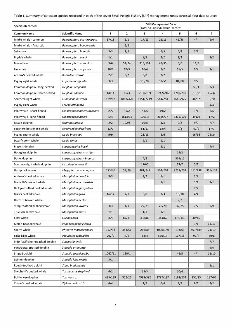
4
Table 1. Summary of cetacean species recorded in each of the seven Small Pelagic Fishery (SPF) management zones across all four data sources
Species Recorded SPF Management Zone
(Total no. individuals/no. records)
Common Name Scientific Name 1 2 3 4 5 6 7
Minke whale - common Balaenoptera acutorostrata 37/18 1/1 17/13 15/15 49/38 4/4 6/6
Minke whale - Antarctic Balaenoptera bonaerensis 2/2
Sei whale Balaenoptera borealis 3/3 2/2 5/3 5/4 3/2
Bryde's whale Balaenoptera edeni 1/1 8/8 2/2 2/2 2/2
Blue whale Balaenoptera musculus 9/6 54/24 318/197 49/35 6/6 11/9
Fin whale Balaenoptera physalus 10/6 10/3 10/4 2/2 18/5 9/7 1/1
Arnoux's beaked whale Berardius arnuxii 2/2 5/2 9/8 2/2
Pygmy right whale Caperea marginata 3/3 20/20 53/51 84/80 9/7
Common dolphin - long-beaked Delphinus capensis 50/1 3/3
Common dolphin - short-beaked Delphinus delphis 14/14 16/3 2190/139 3242/216 1783/261 513/21 45/37
Southern right whale Eubalaena australis 179/18 4867/420 6151/2249 544/284 1660/925 46/82 8/20
Pygmy killer whale Feresa attenuata 4/4
Pilot whale - short-finned Globicephala macrorhynchus 55/2 31/2 44/5 19/2 1/1 6/6
Pilot whale - long-finned Globicephala melas 5/4 1613/32 100/18 2625/77 3314/101 491/9 17/2
Risso's dolphin Grampus griseus 2/2 102/5 10/5 3/3 2/2 9/2 7/7
Southern bottlenose whale Hyperoodon planifrons 12/3 51/17 13/4 9/3 47/9 17/3
Pygmy sperm whale Kogia breviceps 9/9 23/18 6/6 16/16 25/24
Dwarf sperm whale Kogia simus 2/1 1/1
Fraser's dolphin Lagenodelphis hosei 5/1 4/4
Hourglass dolphin Lagenorhynchus cruciger 12/2
Dusky dolphin Lagenorhynchus obscurus 4/2 369/12
Southern right whale dolphin Lissodelphis peronii 170/2 57/7 2/2
Humpback whale Megaptera novaeangliae 273/46 59/29 481/241 504/264 2211/769 411/138 315/109
Andrew's beaked whale Mesoplodon bowdoini 3/3 2/2 1/1 2/2
Blainville's beaked whale Mesoplodon densirostris 1/1 1/1 1/1
Ginkgo-toothed beaked whale Mesoplodon ginkgodens 2/2
Gray's beaked whale Mesoplodon grayi 16/12 2/1 8/8 3/3 10/10 4/4
Hector's beaked whale Mesoplodon hectori 2/2
Strap-toothed beaked whale Mesoplodon layardii 3/3 1/1 27/21 20/20 37/25 7/7 9/9
True's beaked whale Mesoplodon mirus 1/1 1/1 1/1
Killer whale Orcinus orca 66/9 87/11 498/80 344/62 473/140 40/16
Melon-headed whale Peponocephala electra 1/1 13/11
Sperm whale Physeter macrocephalus 352/38 384/51 266/85 1006/140 193/63 591/189 21/10
False killer whale Pseudorca crassidens 207/9 4/4 62/4 556/17 117/18 90/4 80/8
Indo-Pacific humpbacked dolphin Sousa chinensis 7/7
Pantropical spotted dolphin Stenella attenuata 9/6
Striped dolphin Stenella coeruleoalba 1067/11 150/1 46/5 4/4 12/10
Spinner dolphin Stenella longirostris 3/1
Rough-toothed dolphin Steno bredanensis 1/1
Shepherd's beaked whale Tasmacetus shepherdi 6/2 13/3 10/4
Bottlenose dolphin Tursiops sp. 425/139 352/26 4983/392 1797/187 5182/274 155/25 137/65
Cuvier's beaked whale Ziphius cavirostris 4/4 2/2 6/6 8/8 8/3 2/2

5
Short-beaked common and bottlenose dolphins were identified as the cetacean species at greatest
risk of interaction with the fishery (Fitzgerald et al. 2015). Metadata of sighting and stranding
records for these species are presented in further detail for each data source (Table 2), including
spatial and temporal coverage. Both of these species have been recorded within each of the SPF
management zones, though bottlenose dolphins appear to be recorded more frequently in
management zones 1 and 7 than common dolphins (Figures 2 & 3). The AMMC data records span
nationwide and so are the most informative of sightings outside of Tasmania and South Australia.
As other data sources largely focus on these two states, the distribution of records is highly skewed
towards these areas. Overall, a total of 1206 common and 1577 bottlenose dolphin records were
available, spanning a total of 54 and 72 years between 11-Sep-1982 to 06-Jan-2015 and 30-Oct-
1902 to 31-Jan-2014 respectively (Table 2). These records were estimated to include a total of
8,334 common and 13,498 bottlenose dolphin individuals. It is unknown how many records
resighted the same individuals.
The seismic survey data are more systematically recorded than the opportunistic sighting and
stranding records, with some measure of sighting effort. However, these data are not collected in a
manner designed for estimating marine mammal distribution or abundance. The spatial bounds of
seismic surveys are very limited compared to the range of potential cetacean habitat, and the
airguns or other activity may affect the normal behaviour of cetaceans in the area, biasing results.
Observations are also carried out on different platforms, by different observers, in a variety of sea
states, so this presents a challenge in standardising sighting effort across surveys.
Sighting effort was available and assimilated into the NMMDB at the time of this report for a total
of six seismic surveys conducted within the Small Pelagic Fishery region (Table 3). An additional 36
surveys are available through the Cetacean Sightings Application (CSA) version 3 but took place
outside the region of the SPF. Further surveys have been submitted but are beyond the scope of
summary for this report due to the short timeframe. These include electronic records submitted
through CSA version 2 which will be assimilated in the near future, and survey data submitted in
PDF format which will take longer to extract and format. These records will be available in the
future through the National Marine Mammal Data Portal (http://data.marinemammals.gov.au).
During the six available surveys a relatively small number of common dolphins were sighted and all
but one survey sighted no bottlenose dolphins. The results from these six surveys are spatially
biased, with sighting effort largely skewed towards SPF zone 2.
The seasonal spatial distribution and total number of dolphins reported for each record are
presented for each data source in the Appendices (Common dolphin: Appendix 1; Bottlenose
dolphin: Appendix 2). A greater number of common dolphin sightings were of 10 or more
individuals (28%) compared to sightings of bottlenose (7.4%). Sightings of over 50 dolphins were
rare for both species, at 5.7% and 2.9% of all sightings for common and bottlenose dolphins
respectively. Both species were recorded throughout the year, however with no information on
sighting effort it is not possible to draw any conclusions regarding seasonal trends.
Overall, as the majority of these data are opportunistic records collected when a stranding or
sighting of a cetacean is reported, they represent presence-only, non-systematic data on species’

6
distributions. The data can therefore only be used to inform on the potential seasonal locations of
different species, but cannot predict where and when a species is unlikely to be present. Systematic
surveys using designed transect lines with consistent spatial and temporal sighting effort across
species’ habitats are needed to gain an accurate representation of population distribution and
abundance.
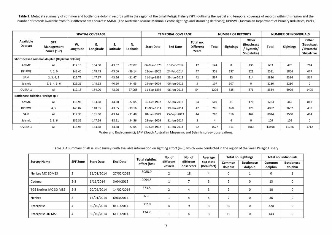
7
Table 2. Metadata summary of common and bottlenose dolphin records within the region of the Small Pelagic Fishery (SPF) outlining the spatial and temporal coverage of records within this region and the
number of records available from four different data sources: AMMC (The Australian Marine Mammal Centre sightings and stranding database); DPIPWE (Tasmanian Department of Primary Industries, Parks,
Water and Environment); SAM (South Australian Museum); and Seismic survey observations.
Table 3. A summary of all seismic surveys with available information on sighting effort (n=6) which were conducted in the region of the Small Pelagic Fishery.
Survey Name SPF Zone Start Date End Date Total sighting
effort (hrs)
No. of different vessels
No. of different observers
Average sea state
(Beaufort)
Total no. sightings Total no. individuals
Common dolphin
Bottlenose dolphin
Common dolphin
Bottlenose dolphin
Nerites MC 3DMSS 2 16/01/2014 27/02/2015 3088.0 2 18 4 0 1 0 1
Ceduna 2-3 1/11/2014 3/04/2015 2094.5 1 7 3 2 0 13 0
TGS Nerites MC 3D MSS 2-3 20/02/2014 14/02/2014 673.5 2 4 3 2 0 10 0
Nerites 3 13/01/2014 6/03/2014 653 1 4 4 2 0 36 0
Enterprise 4 30/10/2014 8/11/2014 602.0 4 9 3 39 0 320 0
Enterprise 3D MSS 4 30/10/2014 6/11/2014 134.2 1 4 3 19 0 143 0
Available Dataset
SPATIAL COVERAGE TEMPORAL COVERAGE NUMBER OF RECORDS NUMBER OF INDIVIDUALS
SPF Management
Zones (1-7)
W. Longitude
E. Longitude
S. Latitude
N. Latitude
Start Date End Date Total no. Different
Years Total Sightings
Other (Beachcast/ Bycatch/ Shipstrike)
Total Sightings
Other (Beachcast/ Bycatch/ Shipstrike
Short-beaked common dolphin (Dephinus delphis)
AMMC All 112.13 154.00 -43.02 -27.07 06-Mar-1979 13-Dec-2012 17 144 8 136 693 479 214
DPIPWE 4, 5, 6 143.40 148.43 -43.66 -39.14 21-Jun-1902 24-Feb-2014 47 358 137 221 2531 1854 677
SAM 2, 3, 4, 5 129.77 147.67 -43.96 -31.47 11-Sep-1892 29-Jun-2013 42 597 83 514 2830 2316 514
Seismic 2, 3, 4, 5, 6 129.29 148.62 -40.56 -34.65 25-Apr-2009 06-Jan-2015 5 107 107 0 2280 2280 0
OVERALL All 112.13 154.00 -43.96 -27.065 11-Sep-1892 06-Jan-2015 54 1206 335 871 8334 6929 1405
Bottlenose dolphin (Tursiops sp.)
AMMC All 113.98 153.68 -44.38 -27.05 30-Oct-1902 22-Jan-2013 64 507 31 476 1283 465 818
DPIPWE 4, 5 143.87 148.55 -43.65 -39.16 11-Nov-1914 19-Jan-2014 42 286 160 126 4082 3652 430
SAM All 117.33 151.30 -43.14 -31.48 01-Jan-1929 25-Sepr-2013 44 780 316 464 8024 7560 464
Seismic 2, 3, 6 132.35 147.24 -38.91 -34.56 25-Apr-2009 31-Jan-2014 3 4 4 0 109 109 0
OVERALL All 113.98 153.68 -44.38 -27.05 30-Oct-1902 31-Jan-2014 72 1577 511 1066 13498 11786 1712

8
Figure 2. Short-beaked common dolphin sighting and stranding records distributed throughout the Small Pelagic Fishery management zones (1-7) from each data source: AMMC (The Australian Marine Mammal
Centre sightings and stranding database); DPIPWE (Tasmanian Department of Primary Industries, Parks, Water and Environment); South Australia Museum; and Seismic survey observations.
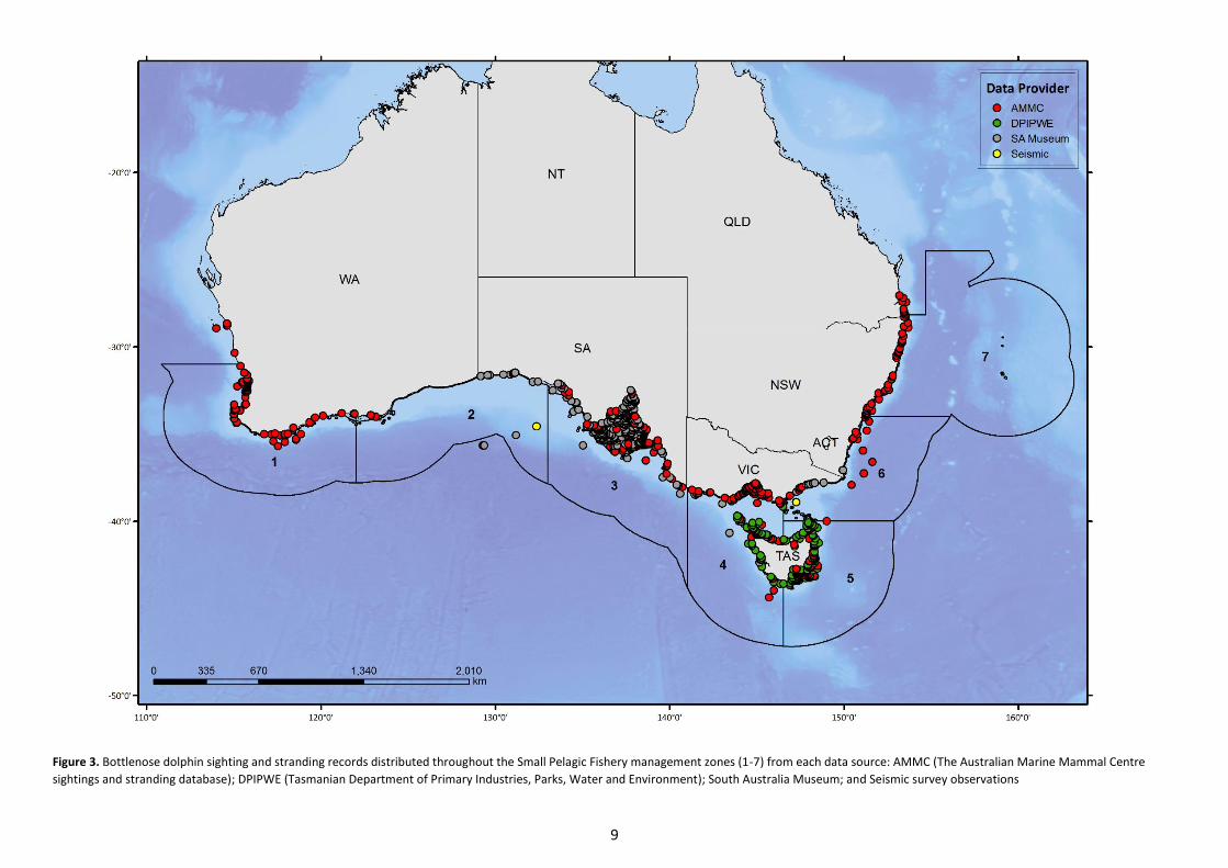
9
Figure 3. Bottlenose dolphin sighting and stranding records distributed throughout the Small Pelagic Fishery management zones (1-7) from each data source: AMMC (The Australian Marine Mammal Centre
sightings and stranding database); DPIPWE (Tasmanian Department of Primary Industries, Parks, Water and Environment); South Australia Museum; and Seismic survey observations
10
Relevant References
AFMA (Australian Fisheries Management Authority) (2015) Small Pelagic Fishery – Assessment report to the
Department of the Environment. July 2015.
Fitzgerald J, Ashby C, Buxton C (2015) Small pelagic research coordination program: Technical workshop to
explore options for mitigating marine mammal interactions in the Small Pelagic Fishery, 2015.
Mackay A, Goldsworthy S (2015) Expert Knowledge Workshop to inform the setting of bycatch trigger limits
for key marine mammal species in the area of the Commonwealth Small Pelagic Fishery – FRDC funded
workshop. SARDI Aquatic Sciences.

11
APPENDIX 1.
Appendix 1.1. Short-beaked common dolphin sighting and stranding records from the AMMC (Australian Marine Mammal Centre) National Sighting and Stranding Database, distributed throughout the Small
Pelagic Fishery management zones (1-7) during summer (n=36) , autumn (n=39), winter (n=28) and spring (n=37).

12
Appendix 1.2. Short-beaked common dolphin sighting and stranding records from the DPIPWE (Tasmanian Department of Primary Industries, Parks, Water and Environment) Cetacean Sighting and Stranding
Database, distributed throughout the Small Pelagic Fishery management zones (1-7) during summer (n=143) , autumn (n=94), winter (n=52) and spring (n=66).

13
Appendix 1.3. Short-beaked common dolphin sighting and stranding records from the SAM (South Australia Museum) Marine Mammal Database, distributed throughout the Small Pelagic Fishery management
zones (1-7) during summer (n=105) , autumn (n=154), winter (n=98) and spring (n=70).

14
Appendix 1.4. Short-beaked common dolphin sighting and stranding records from the seismic survey Cetacean Sightings Application, distributed throughout the Small Pelagic Fishery management zones (1-7)
during summer (n=43) , autumn (n=3), winter (n=1) and spring (n=60).
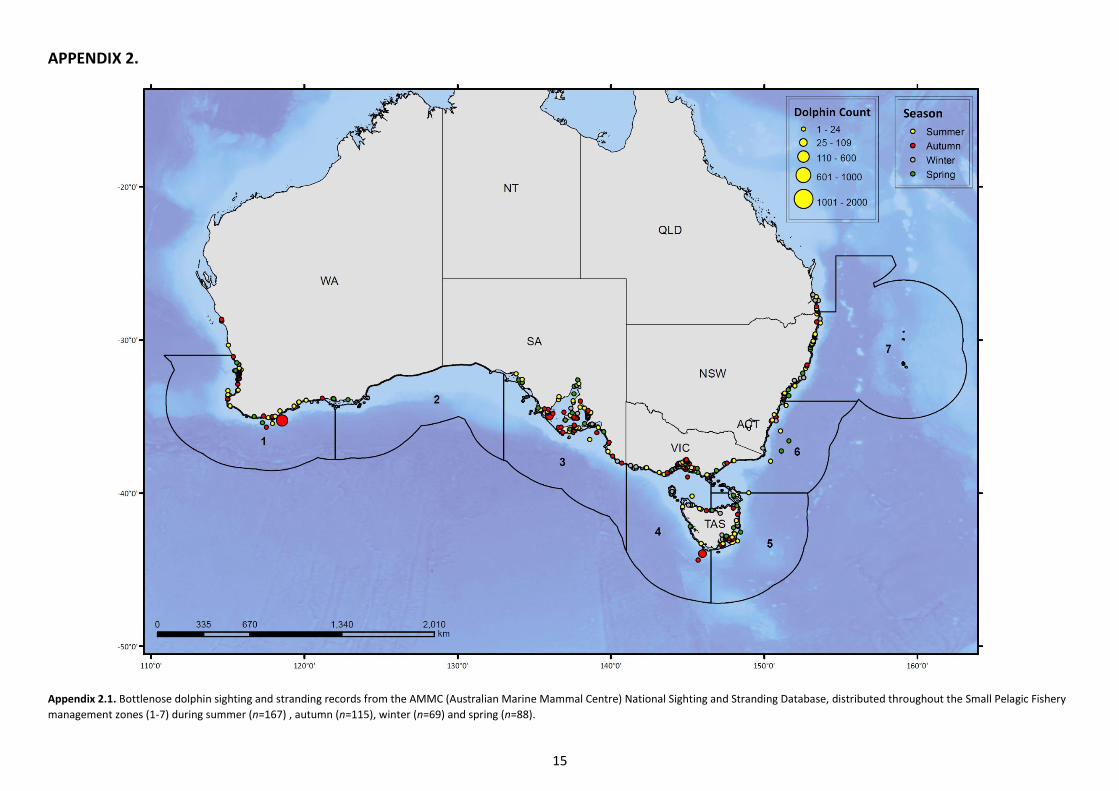
15
APPENDIX 2.
Appendix 2.1. Bottlenose dolphin sighting and stranding records from the AMMC (Australian Marine Mammal Centre) National Sighting and Stranding Database, distributed throughout the Small Pelagic Fishery
management zones (1-7) during summer (n=167) , autumn (n=115), winter (n=69) and spring (n=88).

16
Appendix 2.2. Bottlenose dolphin sighting and stranding records from the DPIPWE (Tasmanian Department of Primary Industries, Parks, Water and Environment) Cetacean Sighting and Stranding Database,
distributed throughout the Small Pelagic Fishery management zones (1-7) during summer (n=77) , autumn (n=61), winter (n=66) and spring (n=80).
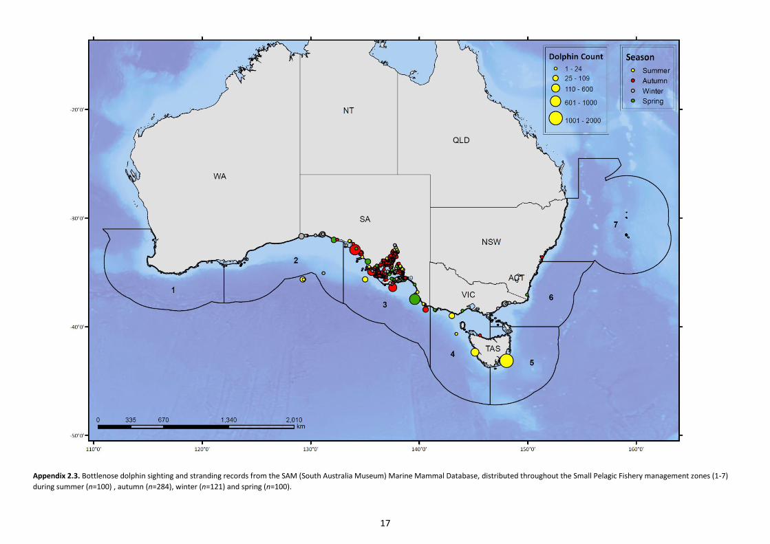
17
Appendix 2.3. Bottlenose dolphin sighting and stranding records from the SAM (South Australia Museum) Marine Mammal Database, distributed throughout the Small Pelagic Fishery management zones (1-7)
during summer (n=100) , autumn (n=284), winter (n=121) and spring (n=100).
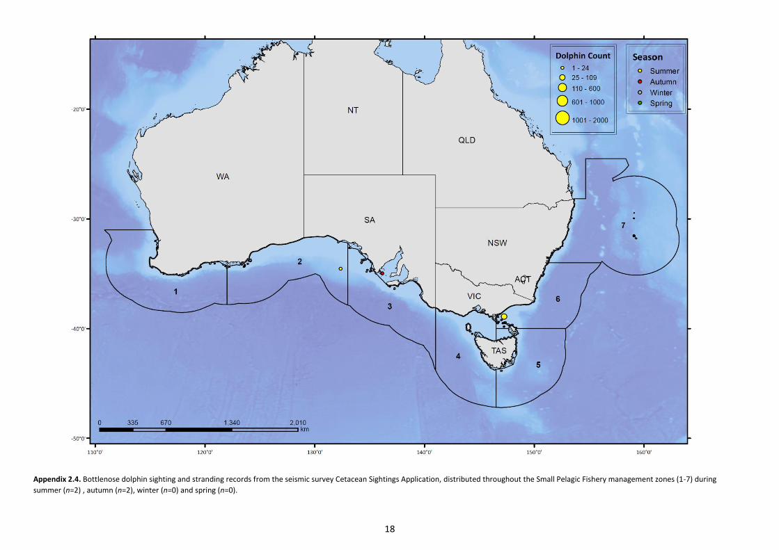
18
Appendix 2.4. Bottlenose dolphin sighting and stranding records from the seismic survey Cetacean Sightings Application, distributed throughout the Small Pelagic Fishery management zones (1-7) during
summer (n=2) , autumn (n=2), winter (n=0) and spring (n=0).

89
Appendix D: Framework for the collection of biological data Draft discussion document regarding the development of a framework for the collection of biological
data from bycaught threatened, endangered and protected (TEP) species.
Biological data from bycaught TEP species can provide important information required for understanding and managing fisheries interactions. This includes the ability to determine the species, population(s), age and sex classes that are being impacted. While current AFMA protocols enable the collection of standard biological measurements of pinnipeds and cetaceans, details regarding the species, population(s), age and sex classes impacted are still lacking.
The move towards Electronic Monitoring across all Commonwealth fisheries means that there will be less observers aboard vessels to collect biological samples and data. Therefore the collection of biological data will increasingly rely on the cooperation of the fishing industry. Because of an increasing reliance on industry involvement, the TEPS interaction sheets for logbook reports to AFMA should form the basis of any biological sampling protocol.
Bycaught individuals will, in general, only be accessible for collection and sampling during the hauling of gear. This is a busy time on a vessel as crew members will have a number of roles to fulfill (depending on the gear) which may include sorting catch, cleaning and reshooting gear. During this time there may be limited opportunity to collect anything but basic data such as species or genus especially if a) the individual is not landed or b) there is no room to retain the individual on deck. There may be opportunities to collect biological samples if the individual can be retained until fishing related duties are completed. Data requests should be prioritized in consultation with industry and other stakeholders bearing in mind time constraints of skippers and crew.
There are a number of key considerations that must be made when requesting and designing a data collection program for industry. If a sampling program is established, there will be a clear need to address the following:
Who will co-ordinate and manage the appropriate permits for data collection from vessels by
industry?
How much time is needed for data collection and how this will be funded?
Will crew members require special training?
If yes, who will provide the training, how will training be funded and what time commitment is required for training?
How will samples be stored?
If physical samples are taken from bycaught individuals how will they be stored (both on the vessel and after the fishing trip)? Who will provide sample collection and storage equipment and how will this be resourced? What will be the mechanism for delivering these to fishing vessels and ensuring supplies are maintained and up to date?
How will samples be collected from vessels?
Samples will need to be able to be deposited at predetermined locations at ports or landing locations. Samples will then need to be transported from these locations to a central repository (e.g. a museum). Again, this process will require co-ordination, funding and management.
Who is responsible for the management of collected samples and how adequate processing, analysis
and reporting on these will be funded?
What will data be used for and how will they be incorporated into management frameworks?
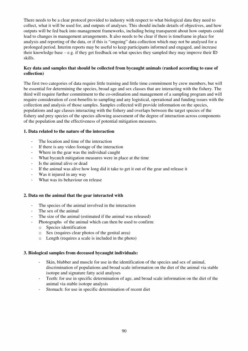
90
There needs to be a clear protocol provided to industry with respect to what biological data they need to collect, what it will be used for, and outputs of analyses. This should include details of objectives, and how outputs will be fed back into management frameworks, including being transparent about how outputs could lead to changes in management arrangements. It also needs to be clear if there is timeframe in place for analysis and reporting of the data, or if this is “ongoing” data collection which may not be analysed for a prolonged period. Interim reports may be useful to keep participants informed and engaged, and increase their knowledge base – e.g. if they get feedback on what species they sampled they may improve their ID skills.
Key data and samples that should be collected from bycaught animals (ranked according to ease of
collection)
The first two categories of data require little training and little time commitment by crew members, but will be essential for determining the species, broad age and sex classes that are interacting with the fishery. The third will require further commitment to the co-ordination and management of a sampling program and will require consideration of cost-benefits to sampling and any logistical, operational and funding issues with the collection and analysis of those samples. Samples collected will provide information on the species, populations and age classes interacting with the fishery and overlaps between the target species of the fishery and prey species of the species allowing assessment of the degree of interaction across components of the population and the effectiveness of potential mitigation measures.
1. Data related to the nature of the interaction
- The location and time of the interaction
- If there is any video footage of the interaction
- Where in the gear was the individual caught
- What bycatch mitigation measures were in place at the time
- Is the animal alive or dead
- If the animal was alive how long did it take to get it out of the gear and release it
- Was it injured in any way
- What was its behaviour on release
2. Data on the animal that the gear interacted with
- The species of the animal involved in the interaction
- The sex of the animal
- The size of the animal (estimated if the animal was released)
- Photographs of the animal which can then be used to confirm: o Species identification o Sex (requires clear photos of the genital area) o Length (requires a scale is included in the photo)
3. Biological samples from deceased bycaught individuals:
- Skin, blubber and muscle for use in the identification of the species and sex of animal, discrimination of populations and broad scale information on the diet of the animal via stable isotope and signature fatty acid analyses
- Teeth: for use in specific determination of age, and broad scale information on the diet of the animal via stable isotope analysis
- Stomach: for use in specific determination of recent diet

91
Appendix E: Workshop Agenda Dates: Monday 19 and Tuesday 20 of October, 2015. SARDI Aquatic Sciences, West Beach, Adelaide
Workshop Agenda
Day 1 - Monday 19 October 2015, convene 09:30 to 17:30 – stakeholders and experts
9:30 – 10:15 Welcome - Professor Gavin Begg (SARDI) Background to workshop – Crispian Ashby (FRDC) Introduction and background to workshop - Professor Peter Harrison (SCU)
10:15 Short coffee break
10:30 – 12: 30 Session 1 Data presentations: Pinnipeds
Australian sea lion and long-nosed fur seal distribution and abundance – Professor Simon Goldsworthy
(SARDI)
Australian fur seal abundance – Dr Peter Shaughnessy (SA Museum)
Australian fur seal at sea distribution – Associate Professor John Arnould (Deakin University)
Question and Answer session
13:00 - 15:00 Session 2 Data presentations: Cetaceans
Presentation of data from the National Marine Mammal Database and Marine Mammal Observer datasets -
Dr Mike Double (Australian Marine Mammal Centre)
Population genetic structure and abundance of short-beaked common dolphins and coastal bottlenose
dolphins in southern and eastern Australia – Associate Professor Dr Kerstin Bilgmann (Flinders University)
Coastal dolphins abundance and genetics – Professor Lars Bejder (Murdoch University)
Question and Answer session
15:00 - 15:30 Coffee break
15:30 - 17:30 Session 3 Background presentations
Overview of Potential Biological Removal (PBR) analysis – Professor Mark Hindell (University of
Tasmania)
Overview of the expert elicitation process – Dr Jan Carey (CEBRA)
Questions and close of workshop to stakeholders
Day 2: Tuesday 20 October 08:30 – 16:00 – closed technical workshop
8:30 First session of expert elicitation
Presentation of results of first elicitation process that was conducted prior to the workshop
Assessment and second elicitation on pinniped data
10:15 Coffee break
10:30 Second session of expert elicitation
Assessment and second elicitation on common dolphin data
12:30 – 13:00 Lunch
13:00 Third session of expert elicitation

92
Assessment and second elicitation on bottlenose dolphin data
15:00 Coffee break
15:15 Fourth session of expert elicitation
Final wrap up and discussions
16:00 Close
List of attending stakeholders Monday 19 October 2015
Representative Organisation
Patrick Hone FRDC
Crispian Ashby FRDC
Brodie Macdonald AFMA
Sally Weekes AFMA
Lynda Bellchambers Department of fisheries WA
Alice Fistr PIRSA
Heidi Alleway PIRSA
Jane McKenzie DEWNR SA
Rachael Alderman DPIPWE, TAS
Mike Double Australian Marine Mammal Centre, Australian Antarctic Division
Allison Runck Commonwealth Department of Agriculture and Water Resources
James Brook Conservation Council SA
Gerry Geen Seafish Tasmania Pty Ltd
Renee Vajtauer Commonwealth Fisheries Association
Marcus Turner South Australian Sardine Industry Association
Paul Watson South Australian Sardine Industry Association
Apologies Organisation
Paul Murphy, Nathan Hanna, Ivan Lawler
Commonwealth Department of the Environment
John Bryan Tasmanian Conservation trust
Alison Webb Department of Economic Development, Jobs, Transport and Resources, VIC
Geoff Allen NSW Department of Primary Industries
Tooni Mahto Australian Marine Conservation Society

93
List of attendees during the closed technical workshop Tuesday 20 October
Attendees Organisation
Peter Harrison (chair) Southern Cross University
Mike Double (morning only) Australian Marine Mammal Centre, Australian Antarctic Division
Mark Bravington CSIRO
Karen Evans CSIRO
John Arnould Deakin University
Jane McKenzie Department of Environment, Water and Natural Resources, SA
Kelly Waples Department of Parks and Wildlife, WA
Sue Mason Dolphin Research Institute
Rachel Alderman DPIPWE
Luciana Möller Flinders University
Kerstin Bilgmann Flinders University
Crispian Ashby (observer) FRDC
Lars Bejder Murdoch University Cetacean Research Unit
Cath Kemper SA Museum
Peter Shaughnessy SA Museum
Mark Hindell University of Tasmania
Simon Goldsworthy SARDI Aquatic Sciences
Alice Mackay SARDI Aquatic Sciences
Sarah-Lena Reinhold (Rapporteur) SARDI Aquatic Sciences
Apologies Organisation
Derek Hamer DBMS Global Oceans
Robert Harcourt Macquarie University
Holly Raudino Department of Parks and Wildlife WA
Peter Gill Blue Whale Study
Mandy Watson Department of Environment and Primary Industries, Vic
Geoff Ross OEH NSW