Cryosphere Part 3: Antarctica

Global Environmental Change – Lecture 7 Spring 2015

Dimensions of Antarctica

• Unlike the Arctic, Antarctica is a continent 14,000,000 km2

• About 98% of Antarctica is covered by ice Averages at least 1.9

kilometers in thickness

• The ice extends to all but the northernmost reaches of the Antarctic Peninsula 2

Gondwana 160 MYBP• Antarctica was part of the Southern

supercontinent known as Gondwana• Around 160 million years ago,

Gondwana began to break up Africa broke off 160 Ma India broke off 125 Ma

Throughout the Cretaceous, Antarctica had a tropical to sub-tropical climate

About 40 M Australia-New Guinea separated from Antarctica

3

Separation of Antarctica• After the breakup, latitudinal currents could isolate Antarctica from Australia,

and the first ice began to appear

• During the Eocene–Oligocene extinction event, about 34 million years ago, CO2 levels were about 760 ppm and had been decreasing from earlier levels in the thousands of ppm

• The collision of India with Asia started to raise the Himalayas, which caused a large increase in the carbonate-silicate cycle, removing CO2 from the atmosphere

• Around 23 Ma, the Drake Passage opened between Antarctica and South America, resulting in the Antarctic Circumpolar Current that completely isolated the continent

4

Full Ice Cover• Models of the changes suggest that declining CO2 levels

became more important

• Ice began to spread over the continent, replacing forests

• Ice has covered most of the continent since about 15 Ma

• The Pleistocene ice-age covered the whole continent and destroyed all major plant life on it

5

Geology of Antarctica• Antarctica is separated into two parts, East and West Antarctica, by the

Gamburtsev Mountains Although these mountains are completely buried by ice, their presence was

first detected by wobbles in the strength of gravity measured from above

East Antarctica is an ancient continental shield Shields are stable, unchanging plateaus at the center of a tectonic plate Normally, they are far from the mountains, like the Gamburtsevs, that occur at

plate boundaries

6

Transantarctic Mountains• Western Antarctica is younger

and more geologically active than its eastern counterpart

• The Transantarctic Mountains, a craggy rock spine that erupts from the ice, marks the boundary between east and west Antarctica

7

Glacial Rebound• GPS data have confirmed that

Antarctica is rebounding from the loss of ice during the last ice age, which ended 12,000 years ago

• The land itself is rising just a few millimeters a year, which is enough to significantly impact calculations of the changing thickness of ice sheets

8

• Transantarctic Mountains, photo by Mike Embree, National Science Foundation

Arctic vs. Antarctic Geography• The Antarctic is almost a

geographic opposite of the Arctic Antarctica is a land mass surrounded

by an ocean, The Arctic is a semi-enclosed ocean,

almost completely surrounded by land

9

Sea Ice• Sea ice is found in remote polar oceans

• On average, sea ice covers about 25 million square kilometers (9,652,553 square miles) of the earth, about two-and-a-half times the area of Canada

• It forms, grows, and melts in the ocean, in contrast to icebergs, glaciers, ice sheets, and ice shelves, which all originate on land

10

Influence on Global Climate• Sea ice influences global climate

Sea ice has a bright surface, so much of the sunlight that strikes it is reflected back into space

Areas covered by sea ice don't absorb much solar energy, so temperatures in polar regions remain relatively cool

If gradually warming temperatures melt sea ice over time, fewer bright surfaces are available to reflect sunlight back into space, more solar energy is absorbed at the surface, and temperatures rise further

This chain of events starts a cycle of warming and melting

11

Ocean Circulation• Sea ice affects the movement of ocean waters

• When sea ice forms, most of the salt is pushed into the ocean water below the ice, although some salt may become trapped in small pockets between ice crystals

• Water below sea ice has a higher concentration of salt and is more dense than surrounding ocean water, which causes it to sink

• In this way, sea ice contributes to the ocean's global "conveyor-belt" circulation

• Cold, dense, polar water sinks and moves along the ocean bottom toward the equator, while warm water from mid-depth to the surface travels from the equator toward the poles

• Changes in the amount of sea ice can disrupt normal ocean circulation, thereby leading to changes in global climate

12

Sea-ice vs. Freshwater Ice• Sea ice forms from salty ocean water, whereas icebergs,

glaciers, and lake ice form from fresh water or snow

• Sea ice grows, forms, and melts strictly in the ocean

• Glaciers are considered land ice, and icebergs are chunks of ice that break off of glaciers and fall into the ocean

• Lake ice is made from fresh water and freezes as a smooth layer, unlike sea ice, which develops into various forms and shapes because of the constant turbulence of ocean water

13

Fresh Water Ice Development• Fresh water is unlike most

substances because it becomes less dense as it nears the freezing point.

• This difference in density explains why ice cubes float in a glass of water

14

• Very cold, low-density fresh water stays at the surface of lakes and rivers, forming an ice layer on the top

Slow Formation of Sea-ice• Salt in ocean water causes the density of the water to increase as it nears

the freezing point, and very cold ocean water tends to sink

• As a result, sea ice forms slowly, compared to freshwater ice, because salt water sinks away from the cold surface before it cools enough to freeze

• The freezing temperature of salt water is lower than fresh water; ocean temperatures must reach -1.8 C to freeze

• Because oceans are so deep, it takes longer to reach the freezing point, and generally, the top 100 to 150 meters of water must be cooled to the freezing temperature for ice to form

15

Behavior of Arctic Ice• Sea ice that forms in the Arctic is not as mobile as sea ice in the

Antarctic

• Sea ice moves around the Arctic basin, but it tends to stay in the cold Arctic waters Floes are more prone to converge, or bump into each other, and pile up into thick

ridges These converging floes makes Arctic ice thicker The presence of ridge ice and its longer life cycle leads to ice that stays frozen longer

during the summer melt So some Arctic sea ice remains through the summer and continues to grow the

following autumn

16

Behavior of Antarctic Ice• Open ocean allows the forming sea ice to move more freely,

resulting in higher drift speeds

• Antarctic sea ice forms ridges much less often than sea ice in the Arctic

• Because there is no land boundary to the north, the sea ice is free to float northward into warmer waters where it eventually melts

• As a result, almost all of the sea ice that forms during the Antarctic winter melts during the summer.

17

Ice Thickness• Because sea ice does not stay in the Antarctic as long as it does

in the Arctic, it does not have the opportunity to grow as thick as sea ice in the Arctic

• Thickness varies significantly within both regions Antarctic ice is typically 1 to 2 meters (3 to 6 feet) thick, Most of the Arctic is covered by sea ice 2 to 3 meters (6 to 9 feet) thick, and

some Arctic regions are covered with ice that is 4 to 5 meters (12 to 15 feet) thick

However, the thick, multiyear ice has been disappearing in the Arctic

18

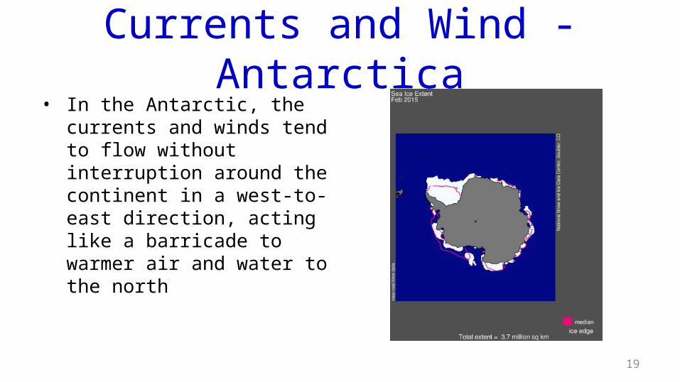
Currents and Wind - Antarctica• In the Antarctic, the currents and

winds tend to flow without interruption around the continent in a west-to-east direction, acting like a barricade to warmer air and water to the north

19

Currents and Wind – Arctic Region• In contrast, the Arctic region north of the

Atlantic Ocean is open to the warmer waters from the south, because of the way the ocean currents flow These warmer waters can flow into the Arctic and

prevent sea ice from forming in the North Atlantic The waters off the eastern coasts of Canada and

Russia are affected by cold air moving off the land from the west

The eastern Canadian coast is also fed by southward-flowing cold water currents that make it easier for sea ice to grow

20

Snowfall• The Arctic Ocean is mostly covered by ice, and surrounded by

land, precipitation is relatively rare Snowfall tends to be low, except near the ice edge

• Antarctica, however, is entirely surrounded by ocean, so moisture is more readily available along the coastline

• Antarctic sea ice tends to be covered by thicker snow, which may accumulate to the point that the weight of snow pushes the ice below sea level, causing the snow to become flooded by salty ocean waters

21

Fresh Water in the Arctic• Water from the Pacific Ocean and several rivers in Russia and

Canada, as well as ice meltwater, provide fresher, less dense water to the Arctic Ocean

• So the Arctic Ocean has a layer of cold, fresh water near the surface with warmer, saltier water below

• This cold, fresh water layer typically allows more ice growth in the Arctic than the Antarctic

22

Ice Sheets, Ice Caps• An ice sheet is a mass of glacial land ice extending more than 50,000 km2

• An ice cap is a dome-shaped mass of glacier ice that spreads out in all directions and is less than 50,000 km2

• The two ice sheets on Earth today cover most of Greenland and Antarctica. During the last ice age, ice sheets also covered much of North America and

Scandinavia. The Antarctic Ice Sheet extends almost 14 million square kilometers, roughly

the area of the contiguous United States and Mexico combined The Antarctic Ice Sheet contains 30 million cubic kilometers of ice If the Antarctic Ice Sheet melted, sea level would rise by about 60 meters

23

Mass Balance in Ice Sheets• Ice sheets are constantly in motion, slowly flowing downhill

under their own weight

• Near the coast, most of the ice moves through relatively fast-moving outlets called ice streams, glaciers, and ice shelves

• As long as an ice sheet accumulates the same mass of snow as it loses to the sea, it remains stable

24

Ice Terminology• An ice stream is a current of ice in an ice sheet or ice cap that flows faster

than the surrounding ice

• A glacier is a mass of ice that originates on land, usually having an area larger than one tenth of a square kilometer; many believe that a glacier must show some type of movement; others believe that a glacier can show evidence of past or present movement

• An ice shelf is a portion of an ice sheet that spreads out over water

• An iceberg is a piece of ice that has broken off from the end of a glacier that terminates in water

25

Antarctic Warming• Most of Antarctica has yet to see dramatic warming

However, the Antarctic Peninsula, which juts out into warmer waters north of Antarctica, has warmed 2.5 degrees Celsius since 1950.

A large area of the West Antarctic Ice Sheet is also losing mass, probably because of warmer water deep in the ocean near the Antarctic coast

In East Antarctica, no clear trend has emerged, although some stations appear to be cooling slightly

Overall, scientists believe that Antarctica is starting to lose ice, but so far the process has not become as quick or as widespread as in Greenland

26

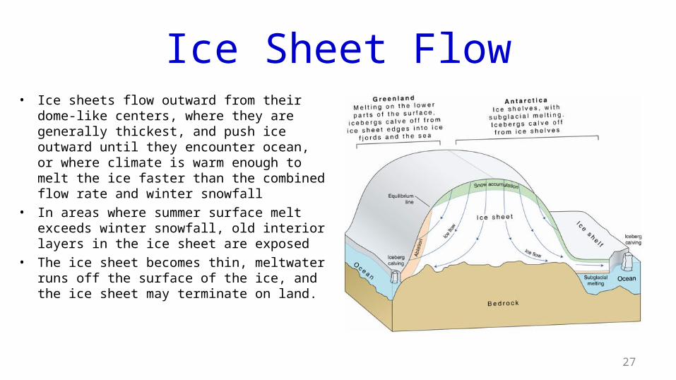
Ice Sheet Flow• Ice sheets flow outward from their dome-

like centers, where they are generally thickest, and push ice outward until they encounter ocean, or where climate is warm enough to melt the ice faster than the combined flow rate and winter snowfall

• In areas where summer surface melt exceeds winter snowfall, old interior layers in the ice sheet are exposed

• The ice sheet becomes thin, meltwater runs off the surface of the ice, and the ice sheet may terminate on land.

27

Ice flow into Oceans• Alpine glaciers may terminate as tidewater

glaciers, ice tongues, or ice shelves Tidewater glaciers terminate by flowing

into the ocean, generally calving ice into the ocean

An ice tongue is a projection of the ice edge up to several km in length caused by wind and current; usually forms when a valley glacier moves very quickly into a lake or ocean

Ice shelves are fully floating thick permanent ice above the ocean

28

Ice Sheet Weather

• Most of the moisture and energy in a storm is in the lower part of the atmosphere

• As a storm approaches an ice sheet, it encounters the steep slopes of the ice sheet edges, and the air is lifted and cooled This leads to heavy blizzards and snowfall along the ice sheet margins. By the time the air masses reach the center of the ice sheet, they are stripped of

most of their moisture. As a result, snow accumulation is typically very low near the summit of an ice

sheet.

29

Ice Sheet “Walls”• Like a wall or

building in the wind, the large bulk of an ice sheet can redirect storms around the ice sheet

30

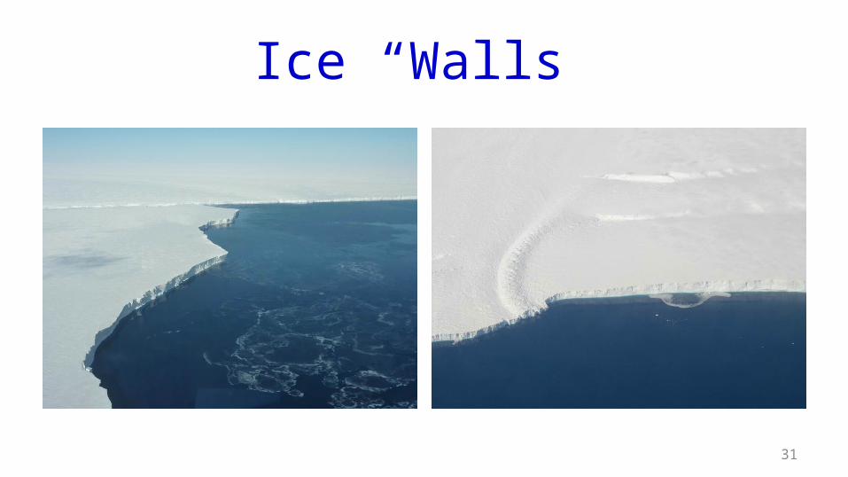
Ice “Walls”

31

Central Ice Sheet Weather

32

• Over the high-elevation center of an ice sheet, the air is typically dry, and skies are clear

• Heat radiates to space from the ice sheet surface because low humidity means less IR absorption

• This chills the surface and the layer of air just above the ice, creating an layering of cold, dense air near the ice surface and warmer air above

• Gravity then pulls the dense layer of cold air downhill

Katabatic Winds• As it flows down the flanks of the ice sheet, the cold air layer picks up

speed

• By the time it reaches the coast, hurricane-force winds, known as katabatic winds, result

• In contrast to coastal storms, katabatic winds can be bone dry

• Cold, dry winds over the surface can lead to ice evaporation of snow and exposure of ice

• "Blue ice" seen in many satellite images results from this process, as do the famous "dry valleys" of Antarctica, where the ice sheet has been completely evaporated away

33

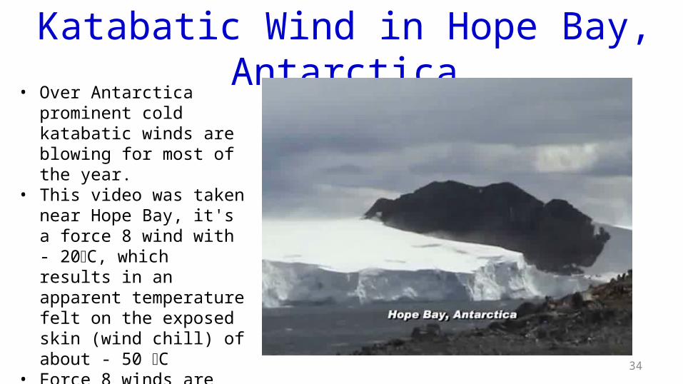
Katabatic Wind in Hope Bay, Antarctica

34

• Over Antarctica prominent cold katabatic winds are blowing for most of the year.

• This video was taken near Hope Bay, it's a force 8 wind with - 20C, which results in an apparent temperature felt on the exposed skin (wind chill) of about - 50 C

• Force 8 winds are gales, with a velocity of 62-74 km/hr

Blue Ice

35

• Blue Ice of Antarctica; courtesy of Brendan van Son

Ice Sheet Mass Balance• Measuring the mass balance of the ice sheets and tracking any

mass balance changes and their causes is very important for forecasting sea level rise

• The mass balance of an ice sheet is the difference between Its total snow input Total loss through melting, ablation, or calving

36

Ice Sheet Mass Balance Measurement • Mass budget method - comparing outflow and melt to

snowfall accumulation

• Volume change or Geodetic method - observing changes in glacier elevation

• Gravimetric method - detecting changes in the Earth’s gravity field over the ice sheet

37

Major Advances in Measurement

38

• 1990s : scientists were unsure of the sign (positive or negative) of the mass balance of Greenland or Antarctica, and knew only that it could not be changing rapidly relative to the size of the ice sheet

• Advances in glacier ice flow mapping using repeat satellite images, and later using interferometric synthetic aperture radar (SAR ) methods, facilitated the mass budget approach, although this still requires an estimate of snow input and a cross-section of the glacier as it flows out from the continent and becomes floating ice.

SAR Technology• A Synthetic Aperture Radar (SAR), is a coherent, mostly airborne or spaceborne,

sidelooking radar system which utilizes the flight path of the platform to simulate an extremely large antenna or aperture electronically, and that generates high-resolution remote sensing imagery

• Over time, individual transmit/receive cycles (PRT's) are completed with the data from each cycle being stored electronically

• The signal processing uses magnitude and phase of the received signals over successive pulses from elements of a synthetic aperture

• After a given number of cycles, the stored data is recombined (taking into account the Doppler effects inherent in the different transmitter to target geometry in each succeeding cycle) to create a high resolution image of the terrain being over flown

39

SAR Capability• By 2002, publications were able to report that both

large ice sheets were losing mass

• In 2010, airborne systems provided resolutions of about 10 cm, with ultra-wideband systems providing resolutions of a few millimeters

40

ICESat and GRACE• In 2003 two new satellites, ICESat and GRACE were launched

• ICESat stands for Ice, Cloud, and land Elevation Satellite

• GRACE stands for Gravity Recovery and Climate Experiment

• These led to vast improvements in one of the methods for mass balance determination, volume change, and introduced the ability to conduct gravimetric measurements of ice sheet mass over time

• The gravimetric method helped to resolve remaining questions about how and where the ice sheets were losing mass

• With this third method, and with continued evolution of mass budget and geodetic methods it was shown that the ice sheets were in fact losing mass at an accelerating rate by the end of the 2000s

41

Mass Balance Results• InSAR observations from 1992 to 2006 mapped the ice flow for most

of the Antarctic coastline In East Antarctica, small glacier losses led to a near-zero loss of 4 ± 61 Gta -1 In West Antarctica, more widespread glacier losses increased ice sheet loss by

59 percent over a decade In 2006, the estimated loss was 132 ± 60 Gt Along the Antarctic Peninsula, losses increased by 140 percent, to 60 ± 46 Gt

in 2006

42

Fig. 1 Antarctic ice velocity derived from ALOS PALSAR, Envisat ASAR, RADARSAT-2, and ERS-1/2 satellite radar interferometry, color-coded on a logarithmic scale, and overlaid on a MODIS mosaic of Antarctica (22), with geographic names discussed in the text.

E Rignot et al. Science 2011;333:1427-1430

Published by AAAS

Geodetic Results - Greenland• From 1997 to 2003, volumetric methods showed that average loss of

ice in Greenland was 80 ± 12 km3 per year

• For 1993-94, the loss was roughly 60 km3 per year

• Causes of the loss About half the increased ice loss was from higher summer melt The rest of the loss resulted from the velocities of some glaciers outstripping

those needed to balance upstream snow accumulation 

• More recent results show a loss of 120 km3 per year

44

Geodetic Results - Antarctica• Recent research showed Antarctica lost overall mass at about 120 gigatons of

ice per year

• Suspected triggers for accelerated ice discharge in both Antarctica and Greenland: Increased surface warning and melt runoff Ocean warming Circulation changes

• During the 21st century it is expected that ice loss will counteract snowfall gains predicted by some climate models 

45

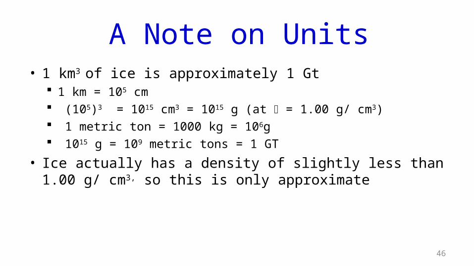
A Note on Units• 1 km3 of ice is approximately 1 Gt

1 km = 105 cm (105)3 = 1015 cm3 = 1015 g (at = 1.00 g/ cm3) 1 metric ton = 1000 kg = 106g 1015 g = 109 metric tons = 1 GT

• Ice actually has a density of slightly less than 1.00 g/ cm3, so this is only approximate

46

ICESat Results• Laser altimetry from ICESat has now supplemented radar altimetry

measurements for more detailed volumetric-based studies.

• In 2009, using ICESat, measurements of both Greenland and Antarctica found that dynamic thinning (ice loss resulting from accelerated glacier flow) now reached all latitudes in Greenland, and had intensified at key areas of Antarctica's grounding line

47

GRACE• GRACE measures changes in the strength of the gravitational

force over the surface of the Earth, including changes driven by the accumulation or loss of ice

48

GRACE Greenland Results• Between April 2002 and April 2006, GRACE data uncovered ice

mass loss in Greenland of 248 ± 36 km3 per year, an amount equivalent to a global sea rise of 0.5 ± 0.1 millimeters per year

• The ice mass loss rate increased by 250 percent between April 2002 to April 2004 and May 2004 to April 2006.

• The increase was due almost completely to increased ice loss rates

in southern Greenland 

49

GRACE Antarctic Results• GRACE measurements indicated a significant ice loss in the

Antarctic Ice Sheet from 2002 to 2005

• Ice sheet mass decreased at 152 ± 80 km3 of ice per year, equal to 0.4 ± 0.2 millimeters of sea level rise per year.

• Most of the mass loss came from the West Antarctic Ice Sheet

50

Data Discrepancies• Glaciologist Robert Bindschadler of NASA's Goddard Space Flight

Center in Greenbelt, Maryland said, “There were so many numbers published out there, how could one not get confused?”

• In the past 15 years, at least 29 studies have estimated how quickly the ice sheets had been losing or gaining mass

• The numbers were all over the map, allowing an overall change in ice sheet mass ranging from a loss of a whopping 676 Gt per year to a gain of 69 Gt

51

Reconciling Data• In 2011, scientists working on the upcoming climate assessment by the

Intergovernmental Panel on Climate Change decided someone had to try something new

• The result was the Ice Sheet Mass Balance Intercomparison Exercise (IMBIE)

• IMBIE had 47 participants from 26 institutions, and was headed by glaciologists Andrew Shepherd of the University of Leeds in the United Kingdom and Erik Ivins of NASA's Jet Propulsion Laboratory in Pasadena, California

• They attempted to make sense of published changes in the ice sheets that were based on four different techniques, each of which gauges the changing amount of ice as snowfall adds ice to an ice sheet and melting and glacier flow to the sea removes it

52

IMBIE Reconciliation • Gains and losses of ice can vary greatly from season to season

and from place to place Surveys made over different, albeit overlapping, time periods and regions

yielded rather different loss rates Once the data were adjusted to uniform regions and periods and a few other

modifications were made, “there's no reason to believe the data sets are saying different things at all,” Shepherd says. “They're showing the same thing.”

53

IMBIE Results• Between 1992 and 2011, the ice sheets each of the regions

listed below changed in mass by Gt a-1 Greenland, -142 ± 49 East Antarctica, +14 ± 43 West Antarctica, -65 ± 26 Antarctic Peninsula -20 ± 14

Since 1992, the polar ice sheets have contributed, on average, 0.59 ± 0.20 millimeter a-1 to the rate of global sea-level rise

54

IMBIE Conclusion• The Richardson et al. paper concluded. “Even the modest rises in ocean

temperature that are predicted over the coming century could trigger substantial ice-sheet mass loss through enhanced melting of ice shelves and outlet glaciers.

• However, these processes were not incorporated into the ice-sheet models that informed the current global climate projections.

• Until this is achieved, observations of ice-sheet mass imbalance remain essential in determining their contribution to sea level.”

55

Snowfall Anomaly• The graph shows the data

from various sources

• In general, there is good agreement

• Note the sharp increase starting around 2009, due to an exceptional snowfall event in East Antarctica

56

• Average anomaly over four drainage basins of Dronning Maud Land in East Antarctica (shaded areas in inset map)

Formation of Antarctica

• Two hundred mybp, Antarctica was part of a supercontinent called Gondwana

• 170 mybp Eastern Gondwana (India, Madagascar, Australia, and Antarctica, drifted to the west of Africa – S. Atlantic Ocean opened

• India drifted N

• 30-40 mybp, Australia and South America moved away, leaving Antarctica about where it is today

57

Drake Passage• Separation of

Chile/Argentina from Antarctica opened the Drake Passage

• This joined the Atlantic and Pacific Oceans

58

Drake Passage Cross-Section• The diagram show a cross-

section between Antarctica and S. America

• This allowed the S. Ocean’s waters free circulation around Antarctica, and created the ACC

59

Antarctic Circumpolar Current• Known as the ACC, this is the world’s largest current

• This current isolated Antarctica, preventing much of the poleward migration of heat from the equator, and turned the Antarctica deep freeze on

• The result has been the largest ice-sheet on earth, containing about 80% of the world’s fresh water

• It also largely isolated the marine organisms of Antarctica from the rest of the world

60

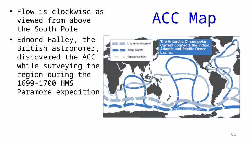
ACC Map• Flow is clockwise as

viewed from above the South Pole

• Edmond Halley, the British astronomer, discovered the ACC while surveying the region during the 1699-1700 HMS Paramore expedition

61

Changes in the ACC• Sarah Gille, from Scripps Institute of Oceanography, reported in

a 2002 Science article that the average mid-depth temperature of the ACC had significantly warmed, and was warming faster than waters in the Atlantic, Indian, and Pacific Oceans

• Fyfe and Saekno (2005) have reported a poleward migration of the ACC about 30 miles since the 1950’s

• They further concluded that, by 2100, shrinkage of the ACC could equal a body of water as large as the Arctic Ocean

62

Shrinking ACC• One outcome of the shrinkage will be an opening for

warm, salty waters from the Indian Ocean to flow into the South Atlantic

• This could greatly influence long-term climate impacts

63

Ice Shelves• Ice shelves already float in the ocean, and therefore they do not

contribute directly to sea level rise when they break up

• However, ice shelf collapse could contribute to sea level rise indirectly

• Ice streams and glaciers constantly push on ice shelves, but the shelves eventually come up against coastal features such as islands and peninsulas, building pressure that slows their movement into the ocean.

64

Consequence of Ice Shelf Collapse• If an ice shelf collapses, the backpressure disappears

• The glaciers that fed into the ice shelf speed up, flowing more quickly out to sea

• Glaciers and ice sheets rest on land, so once they flow into the ocean, they contribute to sea level rise

• The Larsen Ice Shelf, at the north end of the Antarctic Peninsula, has provided recent examples of an ice shelf breakup

65

1995 Breakup of Larsen Ice Shelf • In late January of 1995, a large area, about 2000 square kilometers,

disintegrated into small icebergs during a storm

• At the same time, farther south, a large iceberg broke off the ice shelf front

• Large iceberg calving events are routine for ice shelves, but disintegration is not

• It is hypothesized that the unusual breakup may be a consequence of weakening caused by extreme surface melting during several consecutive warm summer seasons in the 1990's, and by a regional warming over the last few decades

• This was designated the Larsen A Ice Shelf

66

Map• Map of the Larsen Ice shelf

region

• Note the position of James Ross Island for reference

67

British Antarctic Survey (BAS)Image• The "before" picture is taken at 11 GMT,

9/Jan/95

• It is before the iceberg calved, but after the ice shelf between James Ross Island and the peninsula disintegrated

• James Ross Island is the spidery-shaped island slightly above left of the center of the "before" image 

68

BAS Image - After• The "after" is from 12 GMT,

12/Feb/1995

• In this picture the iceberg has calved but has not moved far from where it was calved

69

BAS Image - Later• The 27-2-95 image is 15 days later

• A segment of the ice shelf has broken up and is visible as a plume about 4 times as long as the iceberg

• All images are from near-visible channels and were provided by the ARIES hrpt receiver at Rothera research station

70

Aircraft Photos• Taken by Pete Wragg from within a BAS

twin otter on February 23,1995

• Picture taken approximately 10 km N of Robertson Island, looking WNW

• In the far background the mountains of the Antarctic Peninsula can be seen

71

Cape Longing Photo• Picture taken at Cape Longing, looking

ENE.

• The land in the "foreground" to the left is C. Longing; to the right in middle distance is James Ross Island; in the distance the Peninsula.

• In the center, the channel between James Ross Island and the Mainland is free of shelf ice for the first time in recorded history (which is about 100 years, around here). 

72

SW Tip, James Ross Island• Picture taken over the SW tip of

James Ross Island looking NNW

• In the right foreground, James Ross Island

• In the distance, the Peninsula

• In the middle, the James Ross Channel 

73

Larsen B Breakup• On March 18, 2002 it was

announced that the northern section of the Larsen B ice shelf, a large floating ice mass on the eastern side of the Antarctic Peninsula, has shattered and separated from the continent in the largest single event in a 30-year series of ice shelf retreats in the peninsula

74

2002 Breakup of Larsen B• A total of about 3,250 square kilometers of shelf area disintegrated in a 35-

day period beginning on Jan. 31 of 2002

• Shattered ice formed a plume of thousands of icebergs adrift in the Weddell Sea, east of the Antarctic Peninsula

• Over the 1997-2002 period, the Larsen B shelf has lost a total of 5,700 square kilometers , and is now about 40 percent the size of its previous minimum stable extent

75

Larsen B Breakup• Animation made from still

photos taken 1/31/2002 2/17/2002 2/23/2002 3/07/2002 3/17/2002 4/13/2002

76

• The collapse of the Larsen B Ice Shelf was captured in this series of images from the Moderate Resolution Imaging Spectroradiometer (MODIS) on NASA’s Terra satellite

Larsen Shelf Breakup Effects• The grounded portion of the shelf used to push back against the glaciers,

slowing them down. Without this pushback, the glaciers that fed the ice sheet accelerated and thinned

• Following the spectacular collapse in 2002, the Larsen A and B glaciers experienced an abrupt acceleration, about 300% on average, and their mass loss went from 2–4 Gt a-1 per year between 1996 and 2000, to between 22 and 40 Gt a-1 in 2006

77

Wilkins Ice Shelf Collapse• Farther down the peninsula to the southwest,

the Wilkins Ice Shelf disintegrated in a series of break up events that began in February 2008 (late summer) and continued throughout Southern Hemisphere winter

• The last remnant of the northern part of the Wilkins Ice Shelf collapsed in early April 2009

• It was the tenth major ice shelf to collapse in recent times

78

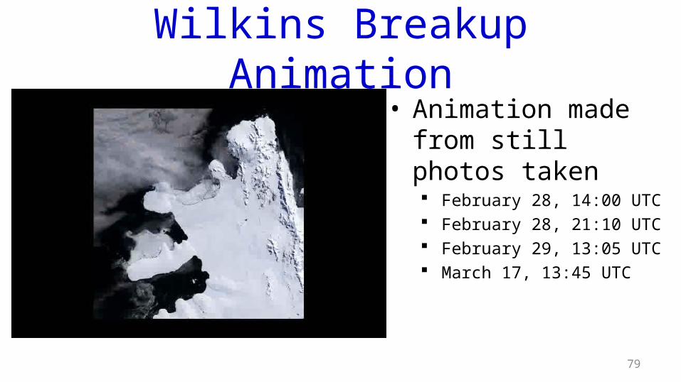
Wilkins Breakup Animation• Animation made from

still photos taken February 28, 14:00 UTC February 28, 21:10 UTC February 29, 13:05 UTC March 17, 13:45 UTC

79

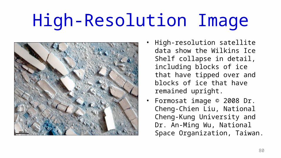
High-Resolution Image• High-resolution satellite data

show the Wilkins Ice Shelf collapse in detail, including blocks of ice that have tipped over and blocks of ice that have remained upright.

• Formosat image © 2008 Dr. Cheng-Chien Liu, National Cheng-Kung University and Dr. An-Ming Wu, National Space Organization, Taiwan.

80

Ice Shelf Differences• The Wilkins Ice Shelf is somewhat unusual in that only the southern end of the shelf

appears to be fed by land-based ice; the rest of the shelf may have formed from accumulation of sea ice that held fast to the coastline through many seasons, as well as snow cover

• Glaciologists estimate that the part of the Wilkins Ice Shelf that formed from sea ice may be 300 to 400 years old, and the part that is fed by glacier flow is older, perhaps up to 1,500 years old

• Because the Wilkins Ice Shelf is only marginally fed by glacier flow, however, its collapse was not expected to have the same impact on sea level rise as the collapse of the Larsen B potentially could

81

Shelf Break-Up Mechanism• Ted Scambos, research scientist at the National Snow and Ice

Data Center in Boulder, Colorado, and his colleagues, Christina Hulbe, associate professor at Portland State University, and Mark Fahnestock, assistant research scientist at the University of Maryland theorized that melt water collecting on the ice shelf surface during unseasonably warm summers might be a primary mechanism in ice shelf breakup

82

Water Cracking Ice• Most ice shelves exhibit some surface melting each summer, but the melting

is usually not widespread enough to affect the structural integrity of the ice

• If summer temperatures are warm enough, significant amounts of melt water can accumulate on ice shelf surfaces, often forming ponds and even streams

• Scambos and Hulbe suspected that excess melt water affected the structural integrity of the ice shelf, particularly in heavily fractured areas.

• “Melt ponds give us a mechanism that makes a nice connection between atmospheric warming and ice shelf disintegration,” said Scambos.

83

Stress Propagation• Hulbe models the effect of melt water on surface crevasses in ice shelves

• Her results showed that melt water, which collects naturally in crevasses, could force even relatively shallow cracks to propagate, or push through, the full thickness of an ice shelf if water continually occupies at least 90 percent of the crevasse

• “When a fracture cracks, it relieves the stress that caused it to crack in the first place. But the tip of that crack becomes a focus at which new stress accumulates, and when the stresses again become large enough to overcome the strength of the ice, the fracture cracks again,” said Hulbe.

84

Water Pressure• In the case of the Larsen B, excessive melt water was

providing the constant stress needed to push fractures through the ice shelf, which was 220 meters thick in places

• The pressure exerted by the melt water is greater than that of the ice, especially if the crevasses are filled with water throughout most of the melt season, as they were on the Larsen B during the 2002 summer season

85

Wilkins 2013• Acquired March 23, 2013, this high-

resolution image from the WorldView-2 satellite shows a portion of the Wilkins Ice Shelf and a large assemblage of icebergs and sea ice just off the shelf front

• Ted Scambos said, “I would not characterize this breakup as a direct result of climate warming, but rather an indirect result of the change in the shape of the shelf.”

86

Use of Satellite Imagery• In 1993, Scambos began monitoring the Antarctic Peninsula using satellite

imagery from the Advanced Very High Resolution Radiometer (AVHRR) sensor

• AVHRR-derived images allowed him to monitor flow features, surface melt water, crevasses, and cracks developing in the ice

• “The AVHRR data set enabled us to build up a pretty good record of the Antarctic coastline, and we could then start speculating about the formation of melt ponds and where the breakups were occurring,” said Scambos

87

MODIS Satellite Imagery• In 2001, Scambos began using NASA’s Moderate Resolution Imaging

Spectroradiometer (MODIS) sensor to monitor the Antarctic Peninsula with even greater detail.

• The MODIS sensor is more sensitive to slight variations in reflected light, making it ideal for imaging ice surfaces.

• “We can see tinier cracks, smaller hills and bumps, and fainter flow features of the ice sheet, which reveals a lot about the flow history of the ice shelf and about whether a specific area is experiencing melting,” said Scambos

88

Additional Ice Shelf Breakup Mechanisms

• David Vaughan, a glaciologist at the British Antarctic Survey in Cambridge, England, suggests that other mechanisms might prove to be equally instrumental in ice shelf breakup.

• “As the ice shelf warms up, the actual strength of the ice may change. Free water between the ice crystals could lubricate and promote fracture growth,” said Vaughan. “And when temperatures are warmer, there’s less sea ice protecting the ice shelf from the ocean swell.”

• Vaughan cites several other possibilities, including possible changes in atmospheric and ocean circulation in the Antarctic region

89

Observation Difficulties• Unlike the melt water fracturing theory, which is easy to monitor using satellite

images, other theories require in situ measurements that can be difficult to obtain.

• A crewmember of the British Antarctic Survey research vessel, James Clark Ross, photographed the aftermath of the Larsen B breakup.

• But according to Vaughan, it was pure luck that the ship happened to be in the area. “Most ship research schedules are determined years in advance, making it virtually impossible for researchers to obtain a ship on short notice. In addition, not all ships have helicopter facilities, meaning researchers can’t be flown ashore,” he said.

90

Ground Based Observation• Tension cracks lined the remaining

Larsen B Ice Shelf south of the Seal Nunataks on March 13, 2002

• Image courtesy of Pedro Skvarca, Instituto Antártico Argentino

• “I don’t think we can look at these other processes using satellite data. If we’re actually trying to see how the material properties of ice shelves change as the temperatures increase, then we actually have to go there,” said Vaughan.

91

Pine Island Glacier (PIG)• The research vessel Nathaniel B Palmer

was investigating the PIG, whose flow speed has increased by over 70%, to around 4 km a-1, since the first observations in the early 1970s

• The accelerations have been accompanied by rapid thinning of the glaciers extending inland from the floating ice shelves that form the glacier termini

92

• One implication of these observed patterns of change is that the mass loss has probably been driven by changes in the rate of submarine melting of the floating ice shelves.

Circumpolar Deep Water• The Palmer had detected the presence of the warm Circumpolar Deep

Water (CDW) on the Amundsen Sea continental shelf, at temperatures 3–4°C above the pressure freezing point in 1994

• In 2009, the Palmer found that submarine melting of PIG had increased by 50% over the intervening 15 years, despite a modest rise in the temperature of CDW of only about 0.1°C

• Documenting the increase in melting from ice front observations was possible, but the reasons remained hidden

93

Using an AUV for Research• During the 2009 cruise, the Palmer

carried an Autosub3, an autonomous underwater vehicle (AUV) capable of accessing and observing the sub-ice cavity

• During the PIG campaign, Autosub3 was launched eight times, including twice for test runs in open water

• It covered a total of 510 km in 94 hours beneath the ice shelf

94

Transverse Ridge• The main outcome of the campaign was the

discovery of a 300 m high submarine ridge lying transverse to the flow of the ice shelf and effectively bisecting the sub-ice cavity

• CDW in Pine Island Bay has free access to the outer cavity, but must clear the ridge to enter the inner cavity where the glacier goes afloat

• The gap above the ridge was less than 300 m, but has grown significantly over recent years as the ice shelf has thinned by nearly 100 m

95

Increasing Gap Size• Positive feedback between the expanding

gap over the ridge, easier access of warm water to the inner cavity, and consequent thinning of the ice may account for much of the observed increase in melting

• The glacier was fully grounded on the ridge sometime prior to the earliest observations

• Its downslope retreat into deeper water has possibly been a self-sustaining process that drove the inland acceleration and thinning

96

Ozone and Climate• When scientists first suggested in the 1970’s that human-produced chemicals could

destroy our ozone shield in the stratosphere, some scientists wondered if ozone and climate could affect each other

• Most nations have been abiding by international agreements to phase out production of ozone-depleting chemicals such as chlorofluorocarbons (CFCs) and halons, and some scientists are predicting the stratospheric ozone layer will recover to 1980 ozone levels by the year 2050

• Well before the expected stratospheric ozone layer recovery date of 2050, ozone’s effects on climate may become the main driver of ozone loss in the stratosphere, resulting in a delay in ozone recovery until 2060 or 2070

97

Stratospheric Cooling• Ozone’s impact on climate consists primarily of changes in temperature.

• The more ozone in a given parcel of air, the more heat it retains

• Ozone generates heat in the stratosphere: By absorbing the sun’s ultraviolet radiation By absorbing upwelling infrared radiation from the lower atmosphere (troposphere).

• Consequently, decreased ozone in the stratosphere results in lower temperatures

• Over recent decades, the mid to upper stratosphere (from 30 to 50 km above the Earth’s surface) has cooled by 1° to 6° C

98

A Question of Timing• Dr. Drew Shindell of the NASA Goddard Institute for Space Studies (GISS) wondered

if stratospheric cooling might result in further depletion of ozone in the stratosphere

• Would the cooling be so fast that even more ozone depletion would occur before the impact of international agreements to limit ozone had time to take effect?

• This might create a possible feedback loop The more ozone destruction in the stratosphere, the colder it would get just because there was less ozone And the colder it would get, the more ozone depletion would occur

99

Polar Ozone Loss• Over both the Arctic and the Antarctic, the deepest ozone

losses result from conditions that occur in the winter and early spring.

• As winter arrives, a vortex of winds develops around the pole and isolates the polar stratosphere.

• The polar vortex is much stronger over Antarctica

100

Polar Stratospheric

Clouds

101

• When temperatures drop below -78°C , thin clouds, composed of water ice, nitric acid, and sulfuric acid mixtures, form – they are called polar stratospheric clouds

• Chemical reactions on the surfaces of ice crystals in the clouds release active forms of CFCs

• These compounds act as catalysts, destroying many ozone molecules for each active CFC created

Ozone Hole Formation• Ozone depletion begins, and the ozone “hole” appears

• In spring, temperatures begin to rise, the ice evaporates, and the ozone layer starts to recover

102

Stratospheric Cooling

103

• The graph shows that the long term average stratospheric temperature declined from the 1981-2010 average, but has remained flat for two decades

• In 2012, the poles experienced warmer-than-average temperatures in the lower stratosphere, especially in the Antarctic region

• This was a response to warmer-than-average temperatures in the troposphere—the layer below the stratosphere.

Ozone Hole Cooling• The ozone hole itself has a minor cooling effect (about 2

percent of the warming effect of GHG’s) because ozone in the stratosphere absorbs heat radiated to space by gases in a lower layer of Earth’s atmosphere (the upper troposphere)

• The loss of ozone means slightly more heat can escape into space from that region

104

A Contrary View• In an article by Baldwin et al. (2007) in Science, they said,

• “Coupled chemistry-climate models include good representations of the stratosphere and interactive ozone chemistry and can therefore simulate changes to the ozone layer and their coupling to climate change. According to these models, ozone recovery will not be a simple reversal of ozone depletion. Rather, the stratospheric cooling from increasing greenhouse gases will accelerate the recovery of the ozone layer, so that pre-1980 ozone abundances are expected to be reached in the middle of this century. The main reason for this acceleration is that most ozone-destroying chemical reactions will be slowed as the stratosphere cools. Beyond 2050, the ozone layer is predicted to become thicker than observed at any time in the last century as the stratosphere continues to cool”

105

Conclusion

More Research is Needed!

106