cs 4487/9587 algorithms for image · pdf filethe university of ontario cs 4487/9587 algorithms...
TRANSCRIPT
The University of
Ontario
CS 4487/9587
Algorithms for Image Analysis
Elements of Image (Pre)-Processing and Feature Detection
Acknowledgements: slides from Steven Seitz, Aleosha
Efros, David Forsyth, and Gonzalez & Woods
The University of
Ontario
CS 4487/9587 Algorithms for Image Analysis
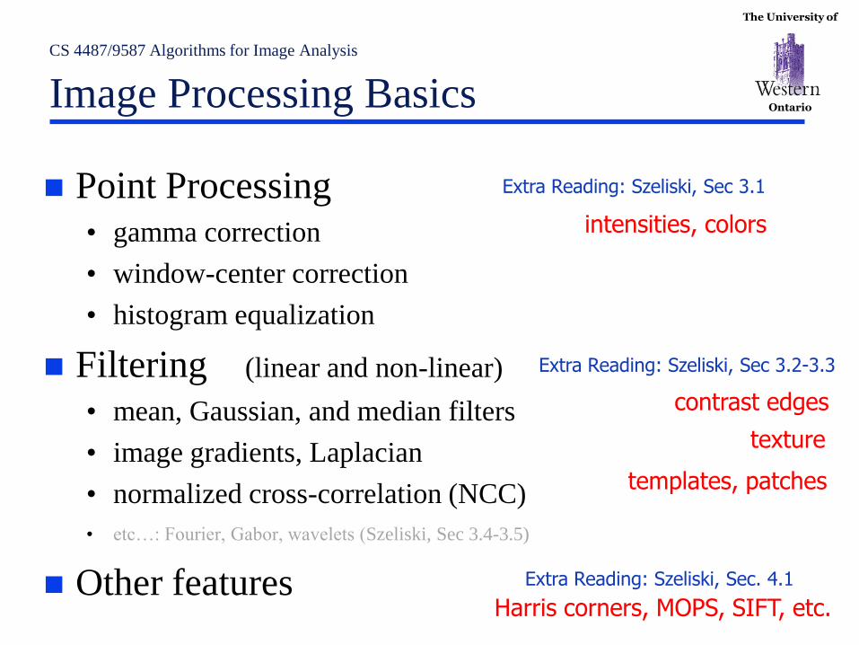
Image Processing Basics
Point Processing • gamma correction
• window-center correction
• histogram equalization
Filtering (linear and non-linear)
• mean, Gaussian, and median filters
• image gradients, Laplacian
• normalized cross-correlation (NCC)
• etc…: Fourier, Gabor, wavelets (Szeliski, Sec 3.4-3.5)
Other features
Extra Reading: Szeliski, Sec 3.1
Extra Reading: Szeliski, Sec 3.2-3.3
Extra Reading: Szeliski, Sec. 4.1
intensities, colors
contrast edges
Harris corners, MOPS, SIFT, etc.
texture
templates, patches
The University of
Ontario Summary of image transformations
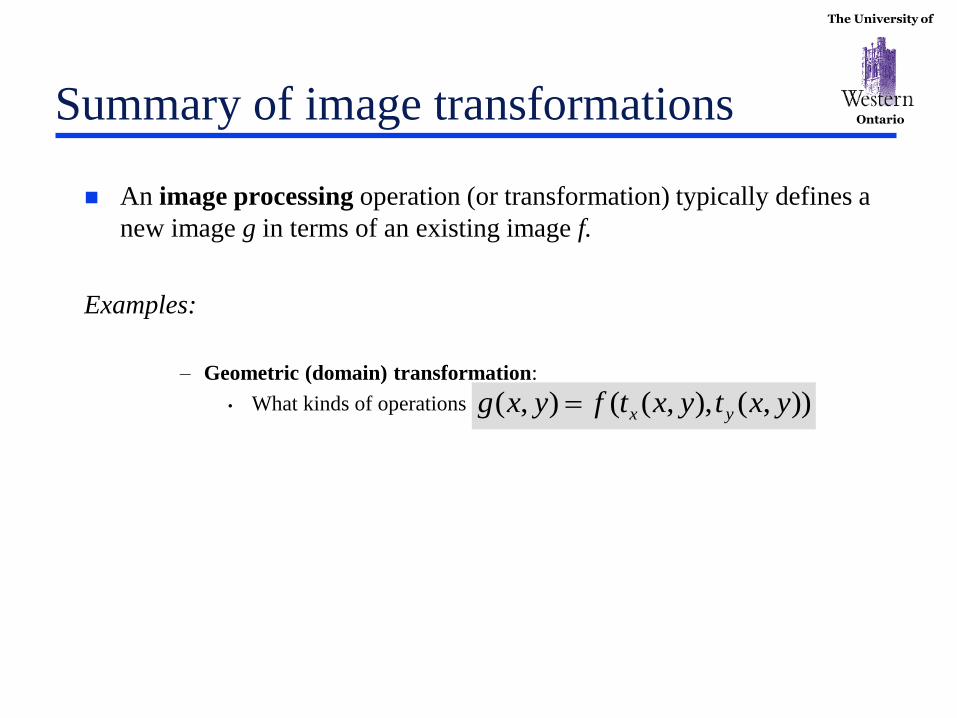
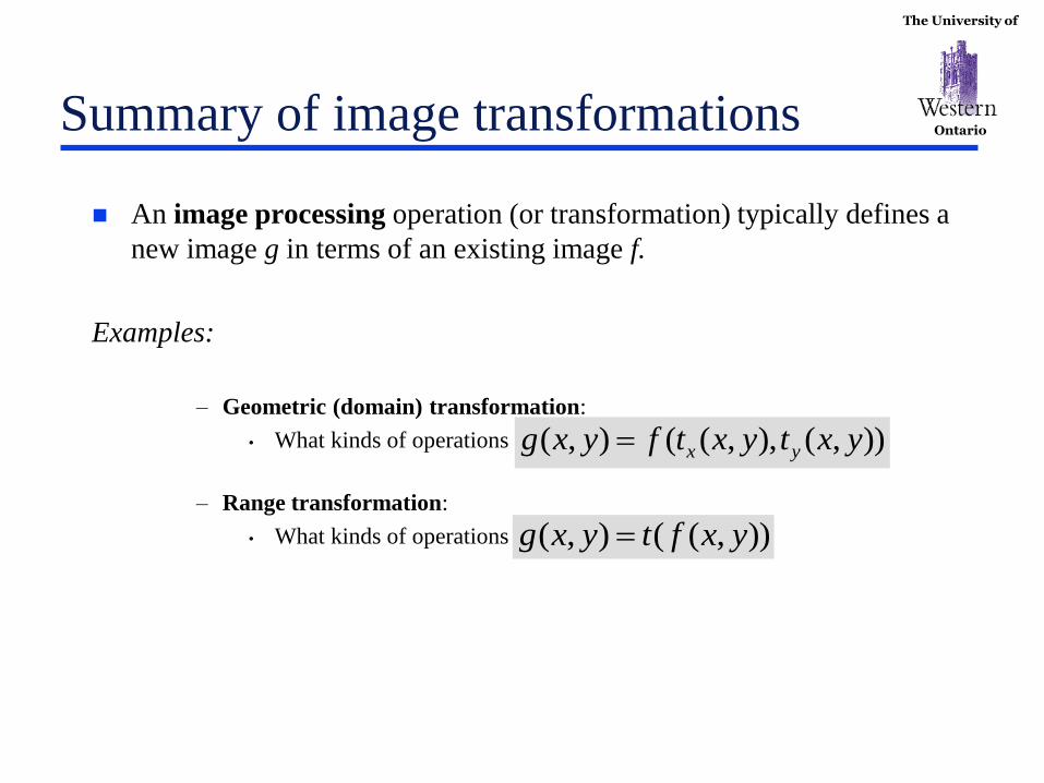
An image processing operation (or transformation) typically defines a
new image g in terms of an existing image f.
Examples:
The University of
Ontario Summary of image transformations
An image processing operation (or transformation) typically defines a
new image g in terms of an existing image f.
Examples:
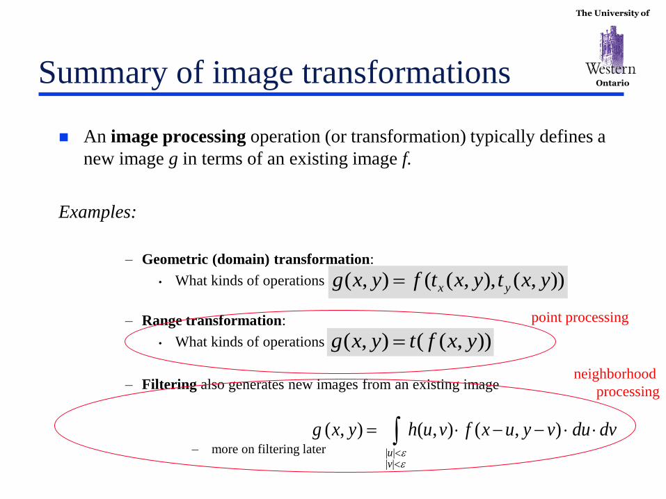
– Geometric (domain) transformation:
• What kinds of operations can this perform?
)),(),,((),( yxtyxtfyxg yx
The University of
Ontario Summary of image transformations
An image processing operation (or transformation) typically defines a
new image g in terms of an existing image f.
Examples:
– Geometric (domain) transformation:
• What kinds of operations can this perform?
– Range transformation:
• What kinds of operations can this perform?
)),(),,((),( yxtyxtfyxg yx
)),((),( yxftyxg
The University of
Ontario Summary of image transformations
An image processing operation (or transformation) typically defines a
new image g in terms of an existing image f.
Examples:
– Geometric (domain) transformation:
• What kinds of operations can this perform?
– Range transformation:
• What kinds of operations can this perform?
– Filtering also generates new images from an existing image
– more on filtering later
)),(),,((),( yxtyxtfyxg yx
dvduvyuxfvuhyxg
vu
||||
),(),(),(
point processing
neighborhood
processing
)),((),( yxftyxg
The University of
Ontario Point Processing
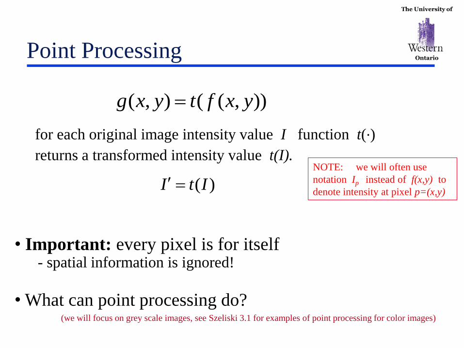
for each original image intensity value I function t(·)
returns a transformed intensity value t(I).
)),((),( yxftyxg
NOTE: we will often use
notation Ip instead of f(x,y) to
denote intensity at pixel p=(x,y)
• Important: every pixel is for itself - spatial information is ignored!
• What can point processing do?
(we will focus on grey scale images, see Szeliski 3.1 for examples of point processing for color images)
)(ItI
The University of
Ontario
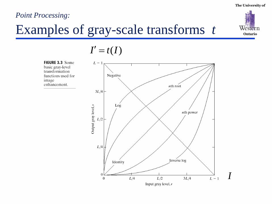
Point Processing:
Examples of gray-scale transforms t
I
)(ItI
The University of
Ontario
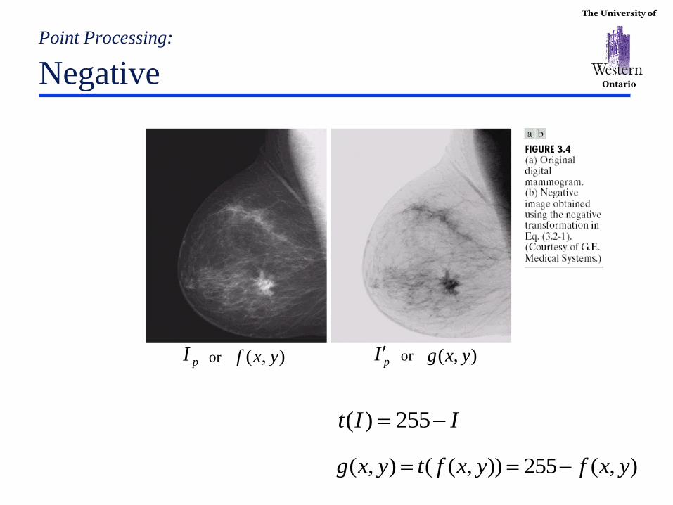
Point Processing:
Negative
),( yxf
),(255)),((),( yxfyxftyxg
IIt 255)(
),( yxgpI or pI or

The University of
Ontario
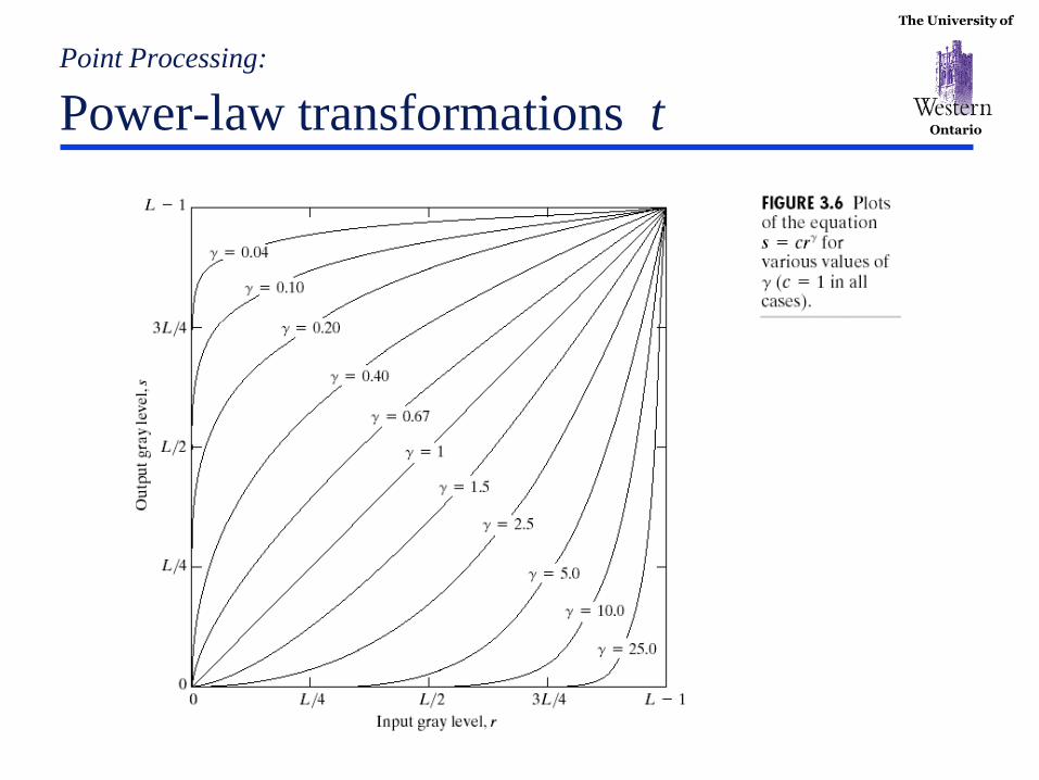
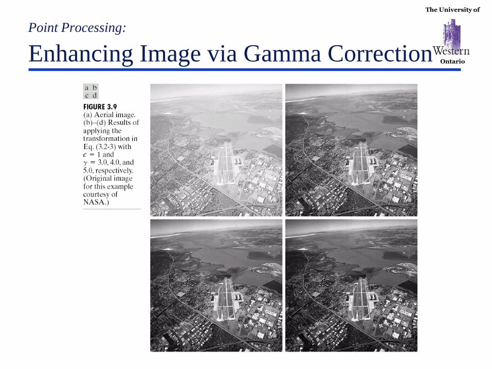
Point Processing:
Gamma Correction
Gamma Measuring Applet:
http://www.cs.berkeley.edu/~efros/java/gamma/gamma.html
The University of
Ontario
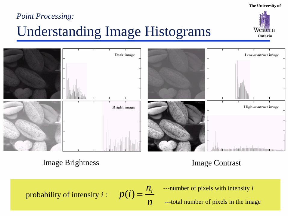
Point Processing:
Understanding Image Histograms
Image Brightness Image Contrast
n
nip i)(probability of intensity i :
---number of pixels with intensity i
---total number of pixels in the image
The University of
Ontario
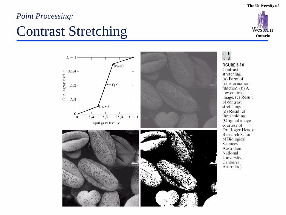
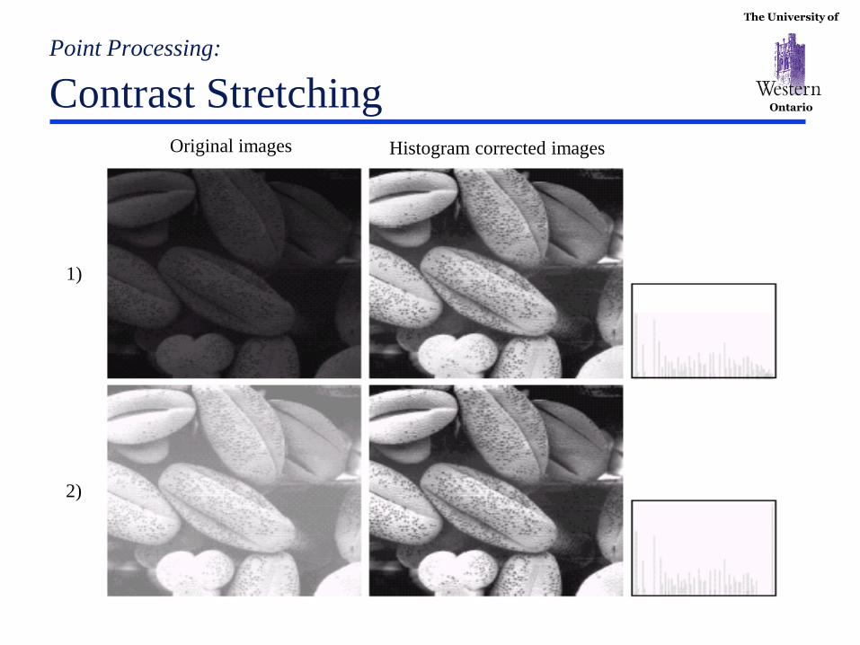
Point Processing:
Contrast Stretching Original images Histogram corrected images
1)
2)
The University of
Ontario
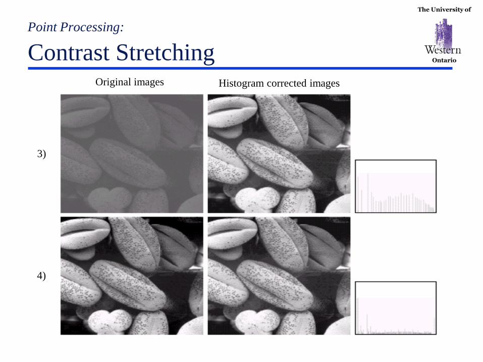
Point Processing:
Contrast Stretching Original images Histogram corrected images
3)
4)
The University of
Ontario
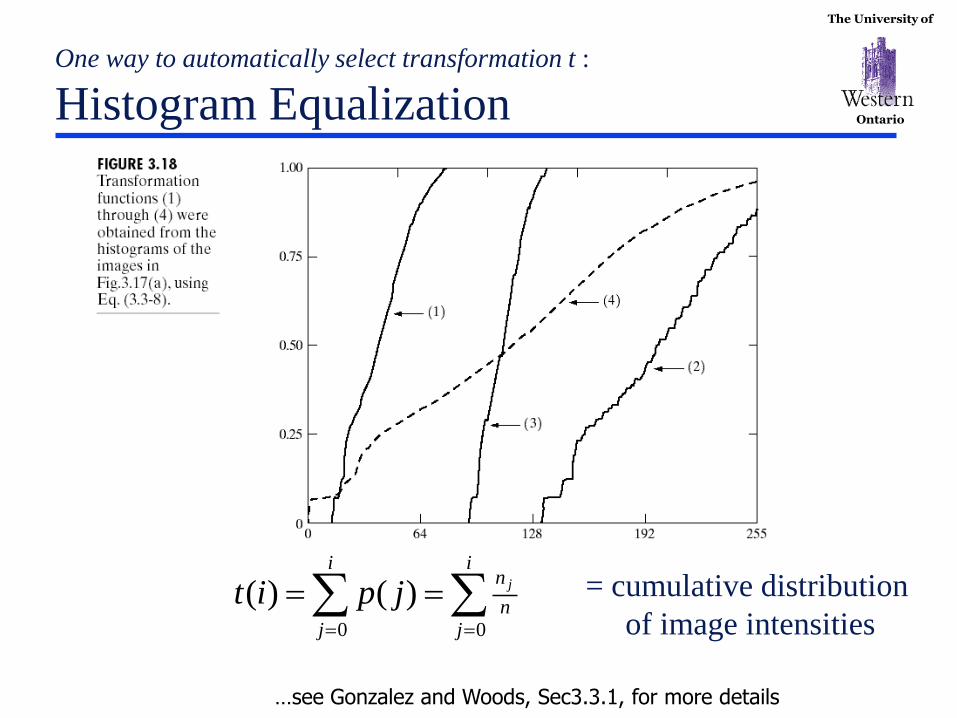
One way to automatically select transformation t :
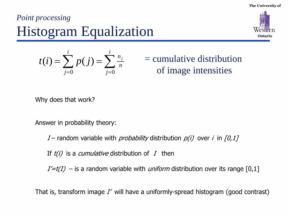
Histogram Equalization
…see Gonzalez and Woods, Sec3.3.1, for more details
= cumulative distribution
of image intensities
i
j
i
j
n
n jjpit0 0
)()(
The University of
Ontario
Point processing
Histogram Equalization
Why does that work? Answer in probability theory: I – random variable with probability distribution p(i) over i in [0,1] If t(i) is a cumulative distribution of I then I’=t(I) – is a random variable with uniform distribution over its range [0,1] That is, transform image I’ will have a uniformly-spread histogram (good contrast)
= cumulative distribution
of image intensities
i
j
i
j
n
n jjpit0 0
)()(

The University of
Ontario
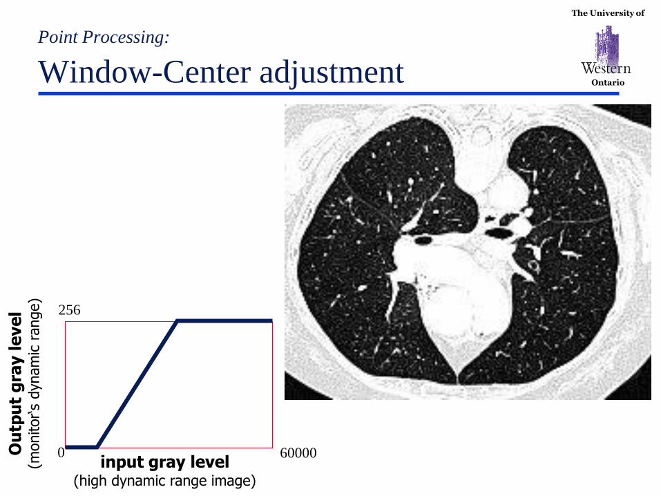
Point Processing:
Window-Center adjustment
input gray level (high dynamic range image)
Ou
tpu
t g
ray l
eve
l (
monitor‘s
dynam
ic r
ange)
0 60000
256
The University of
Ontario
Point Processing:
Window-Center adjustment
input gray level (high dynamic range image)
Ou
tpu
t g
ray l
eve
l (
monitor‘s
dynam
ic r
ange)
0 60000
256
The University of
Ontario
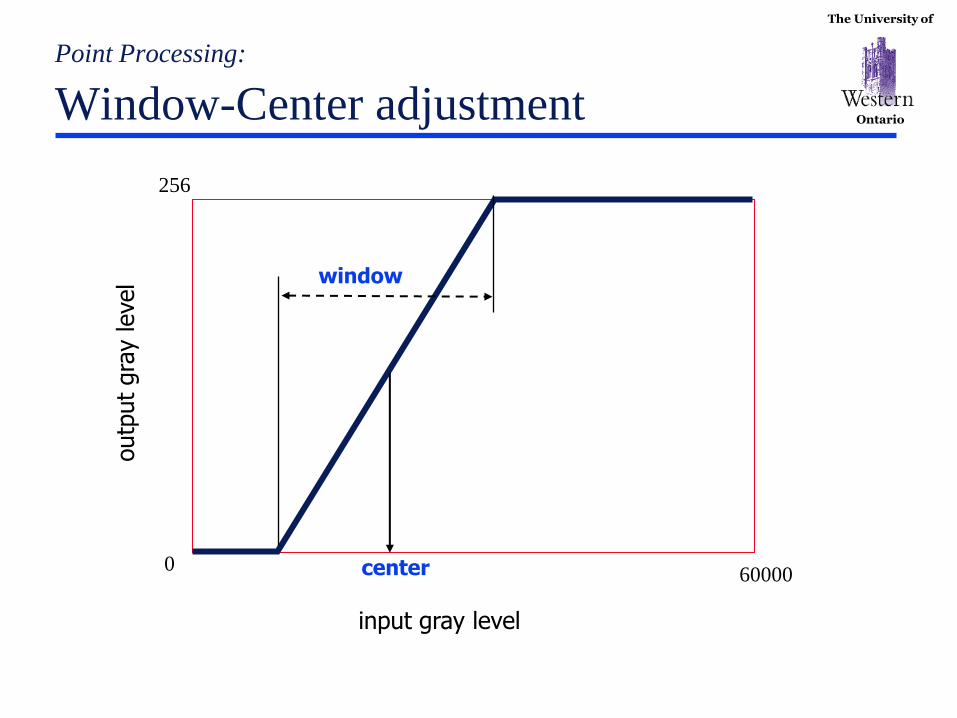
Point Processing:
Window-Center adjustment
input gray level
outp
ut
gra
y level
0 60000
256
center
window
The University of
Ontario
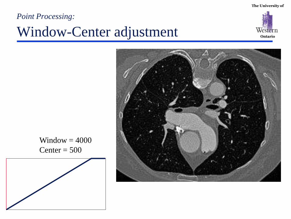
Point Processing:
Window-Center adjustment
Window = 4000
Center = 500

The University of
Ontario
Point Processing:
Window-Center adjustment
Window = 2000
Center = 500
The University of
Ontario
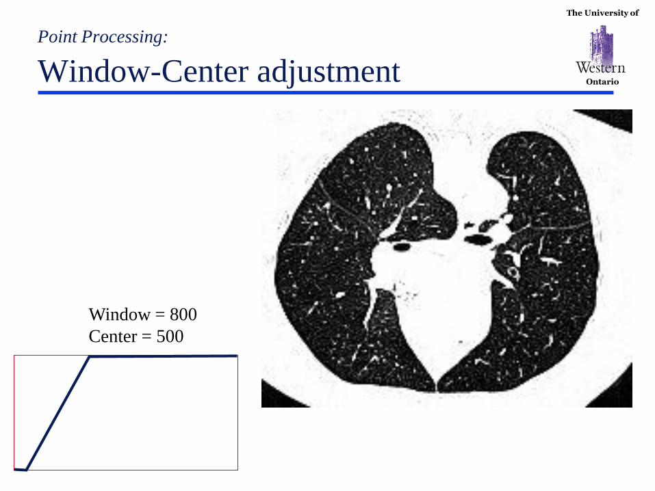
Point Processing:
Window-Center adjustment
Window = 800
Center = 500
The University of
Ontario
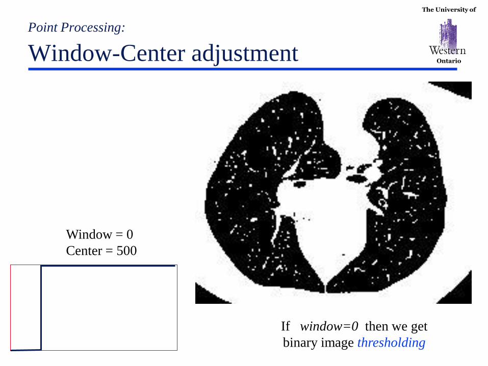
Point Processing:
Window-Center adjustment
Window = 0
Center = 500
If window=0 then we get
binary image thresholding
The University of
Ontario
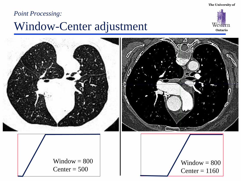
Point Processing:
Window-Center adjustment
Window = 800
Center = 1160
Window = 800
Center = 500
The University of
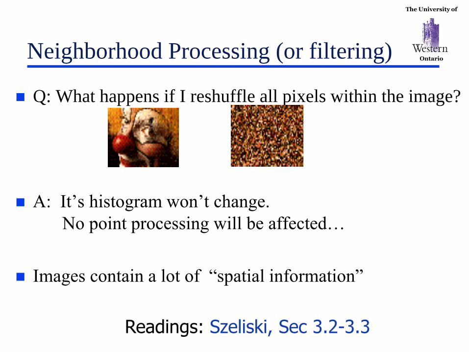
Ontario Neighborhood Processing (or filtering)
Q: What happens if I reshuffle all pixels within the image?
A: It’s histogram won’t change.
No point processing will be affected…
Images contain a lot of “spatial information”
Readings: Szeliski, Sec 3.2-3.3
The University of
Ontario
Neighborhood Processing (filtering)
Linear image transforms
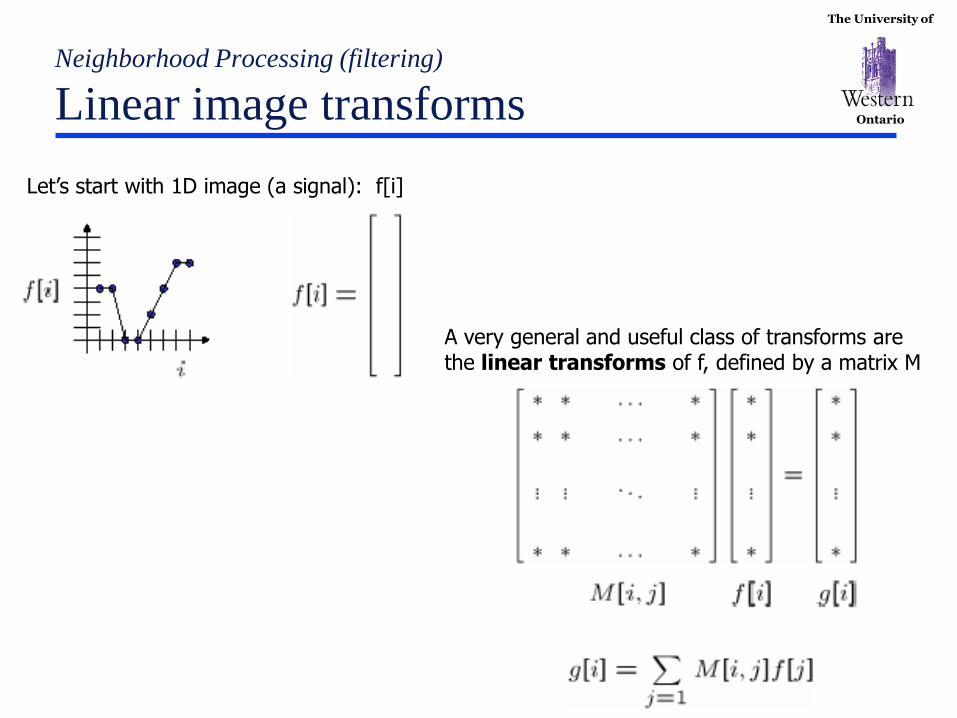
Let’s start with 1D image (a signal): f[i]
A very general and useful class of transforms are the linear transforms of f, defined by a matrix M
The University of
Ontario
Neighborhood Processing (filtering)
Linear image transforms
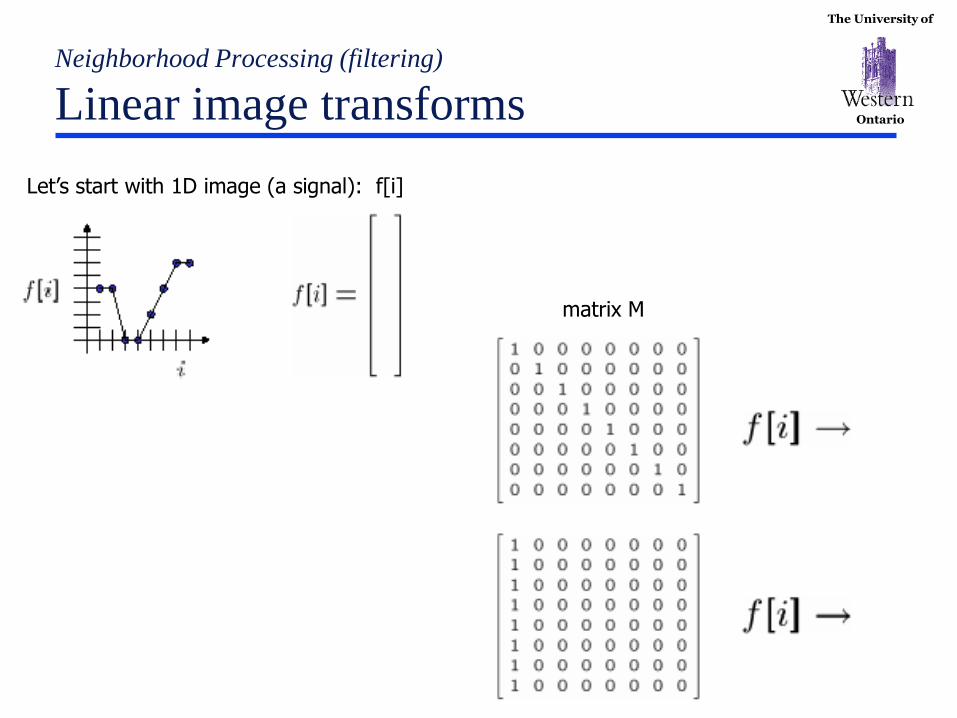
Let’s start with 1D image (a signal): f[i]
matrix M
The University of
Ontario
Neighborhood Processing (filtering)
Linear image transforms
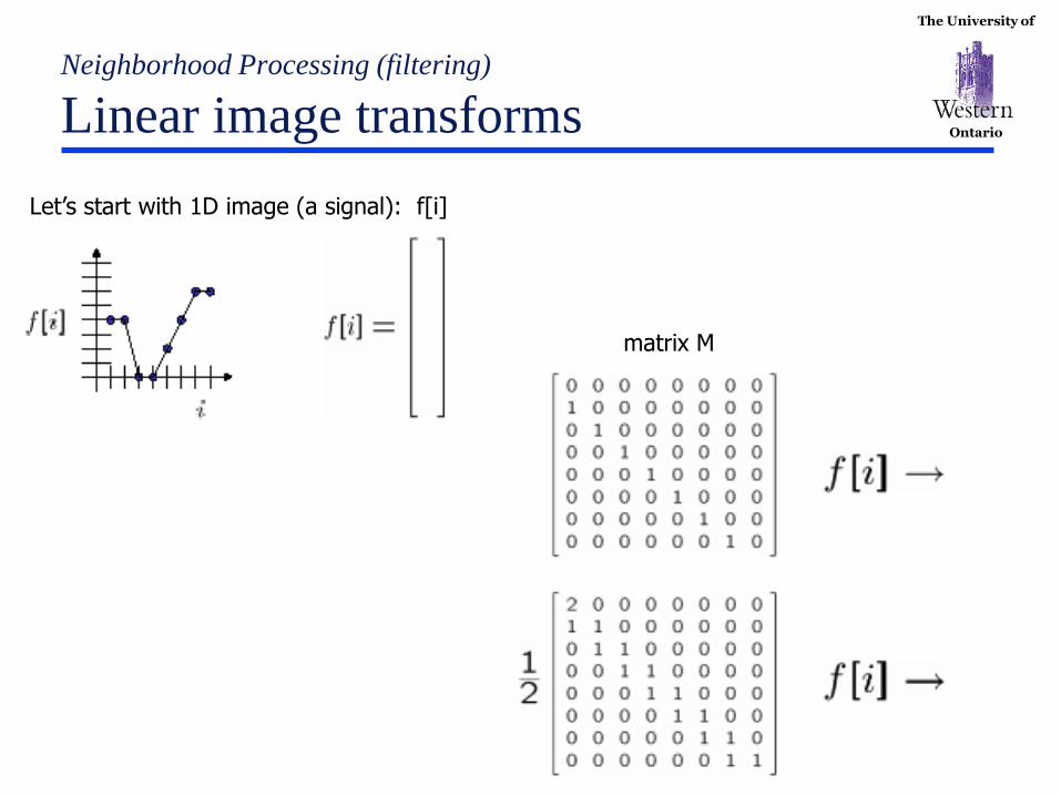
Let’s start with 1D image (a signal): f[i]
matrix M
The University of
Ontario
Neighborhood Processing (filtering)
Linear shift-invariant filters
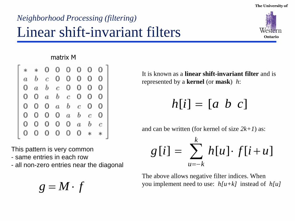
This pattern is very common
- same entries in each row
- all non-zero entries near the diagonal
It is known as a linear shift-invariant filter and is
represented by a kernel (or mask) h:
and can be written (for kernel of size 2k+1) as:
The above allows negative filter indices. When
you implement need to use: h[u+k] instead of h[u]
matrix M
][][ cbaih
k
ku
uifuhig ][][][
fMg
The University of
Ontario
Neighborhood Processing (filtering)
2D linear transforms
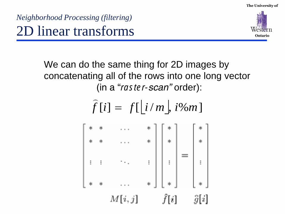
We can do the same thing for 2D images by
concatenating all of the rows into one long vector
(in a “raster-scan” order):
]%,/[][ mimifif
The University of
Ontario
Neighborhood Processing (filtering)
2D filtering
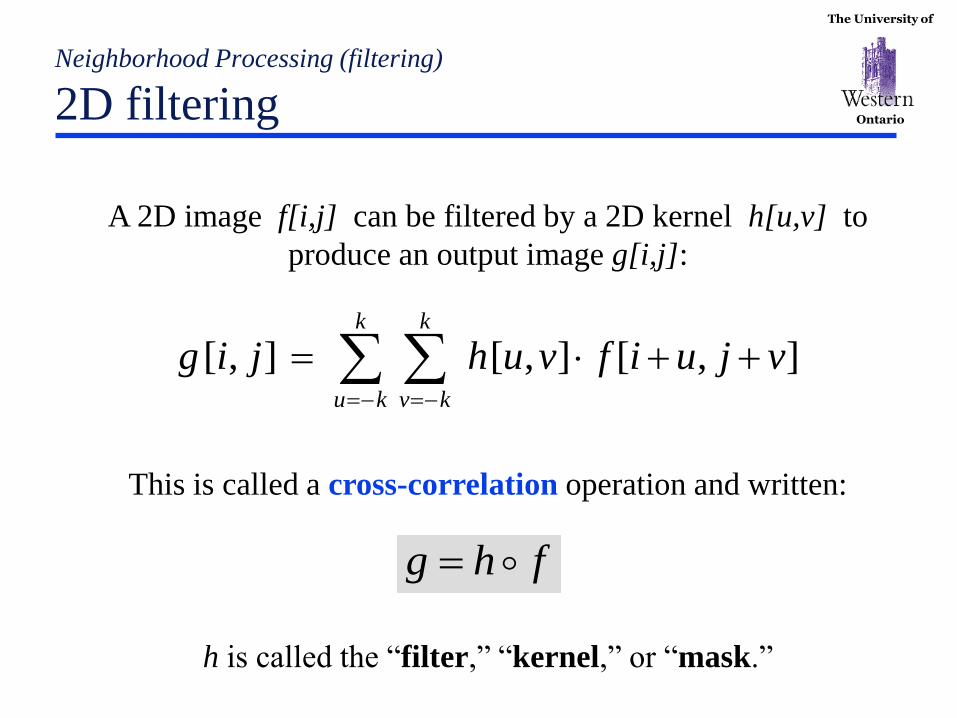
A 2D image f[i,j] can be filtered by a 2D kernel h[u,v] to
produce an output image g[i,j]:
This is called a cross-correlation operation and written:
h is called the “filter,” “kernel,” or “mask.”
fhg
k
ku
k
kv
vjuifvuhjig ],[],[],[
The University of
Ontario
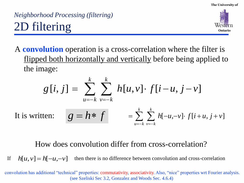
A convolution operation is a cross-correlation where the filter is
flipped both horizontally and vertically before being applied to
the image:
It is written:
How does convolution differ from cross-correlation?
Neighborhood Processing (filtering)
2D filtering
k
ku
k
kv
vjuifvuh ],[],[fhg
k
ku
k
kv
vjuifvuhjig ],[],[],[
If then there is no difference between convolution and cross-correlation ],[],[ vuhvuh
convolution has additional “technical” properties: commutativity, associativity. Also, “nice” properties wrt Fourier analysis.
(see Szeliski Sec 3.2, Gonzalez and Woods Sec. 4.6.4)

The University of
Ontario
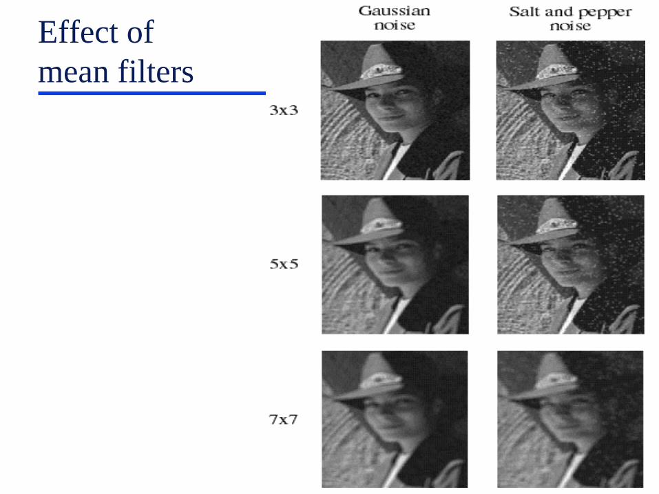
2D filtering
Noise
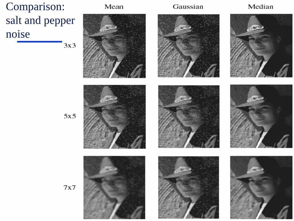
Common types of noise:
• Salt and pepper noise:
random occurrences of
black and white pixels
• Impulse noise: random
occurrences of white pixels
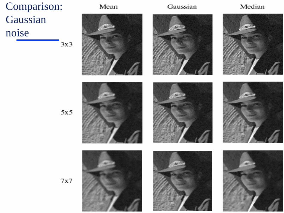
• Gaussian noise: variations in
intensity drawn from a
Gaussian normal distribution
Filtering is useful for
noise reduction...
(side effects: blurring)
The University of
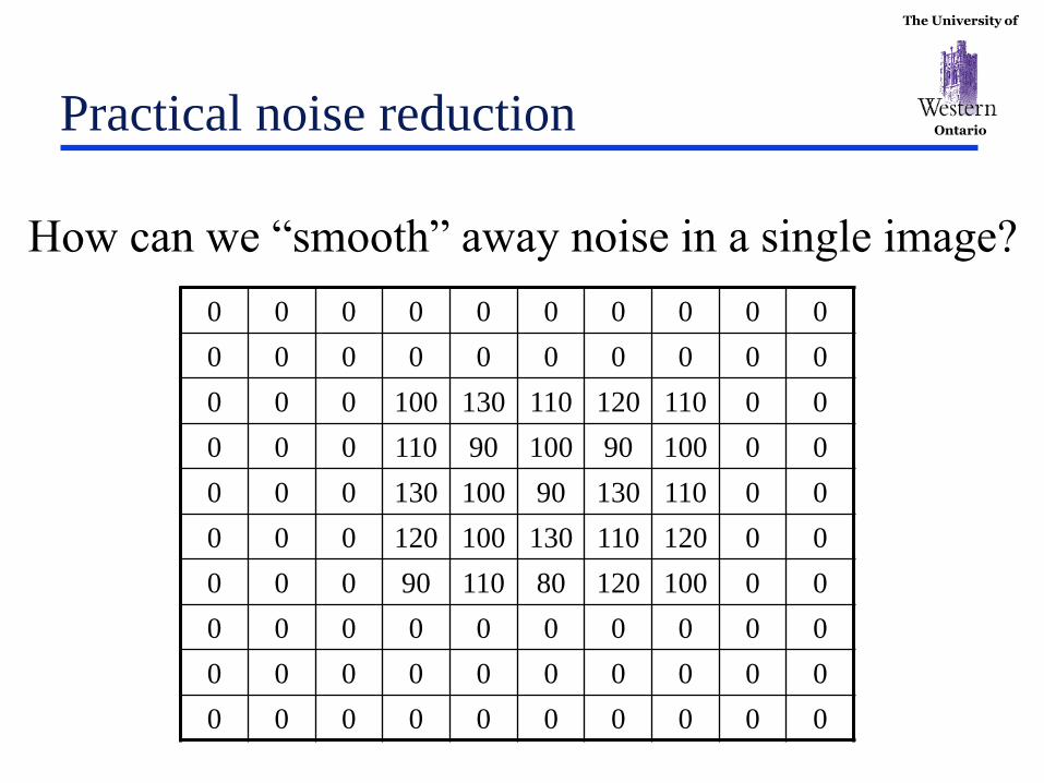
Ontario Practical noise reduction
How can we “smooth” away noise in a single image?
0 0 0 0 0 0 0 0 0 0
0 0 0 0 0 0 0 0 0 0
0 0 0 100 130 110 120 110 0 0
0 0 0 110 90 100 90 100 0 0
0 0 0 130 100 90 130 110 0 0
0 0 0 120 100 130 110 120 0 0
0 0 0 90 110 80 120 100 0 0
0 0 0 0 0 0 0 0 0 0
0 0 0 0 0 0 0 0 0 0
0 0 0 0 0 0 0 0 0 0
The University of
Ontario
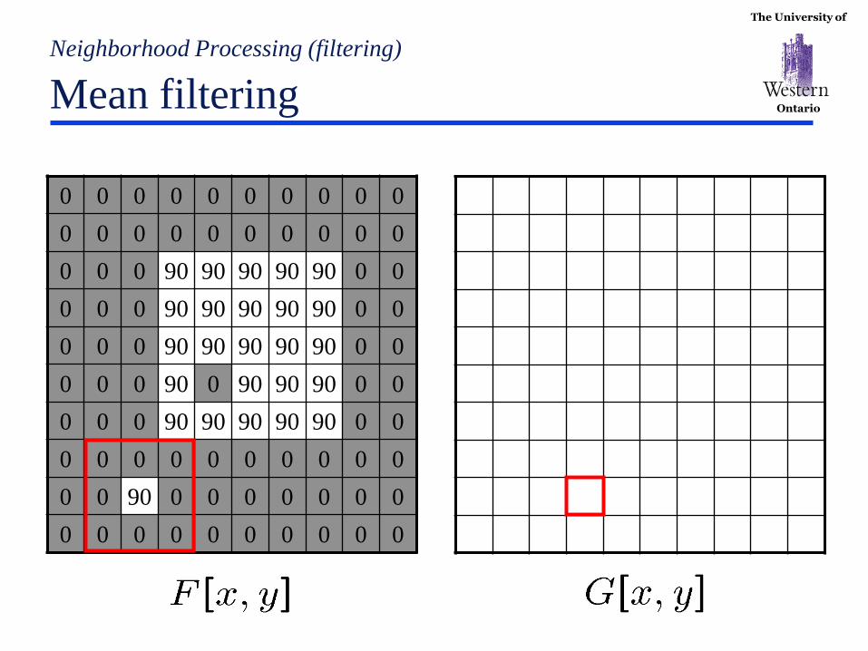
Neighborhood Processing (filtering)
Mean filtering
0 0 0 0 0 0 0 0 0 0
0 0 0 0 0 0 0 0 0 0
0 0 0 90 90 90 90 90 0 0
0 0 0 90 90 90 90 90 0 0
0 0 0 90 90 90 90 90 0 0
0 0 0 90 0 90 90 90 0 0
0 0 0 90 90 90 90 90 0 0
0 0 0 0 0 0 0 0 0 0
0 0 90 0 0 0 0 0 0 0
0 0 0 0 0 0 0 0 0 0
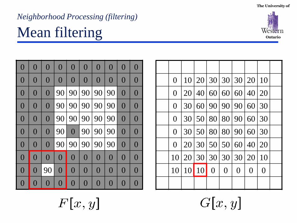
The University of
Ontario
0 0 0 0 0 0 0 0 0 0
0 0 0 0 0 0 0 0 0 0
0 0 0 90 90 90 90 90 0 0
0 0 0 90 90 90 90 90 0 0
0 0 0 90 90 90 90 90 0 0
0 0 0 90 0 90 90 90 0 0
0 0 0 90 90 90 90 90 0 0
0 0 0 0 0 0 0 0 0 0
0 0 90 0 0 0 0 0 0 0
0 0 0 0 0 0 0 0 0 0
Neighborhood Processing (filtering)
Mean filtering
0 10 20 30 30 30 20 10
0 20 40 60 60 60 40 20
0 30 60 90 90 90 60 30
0 30 50 80 80 90 60 30
0 30 50 80 80 90 60 30
0 20 30 50 50 60 40 20
10 20 30 30 30 30 20 10
10 10 10 0 0 0 0 0

The University of
Ontario
Neighborhood Processing (filtering)
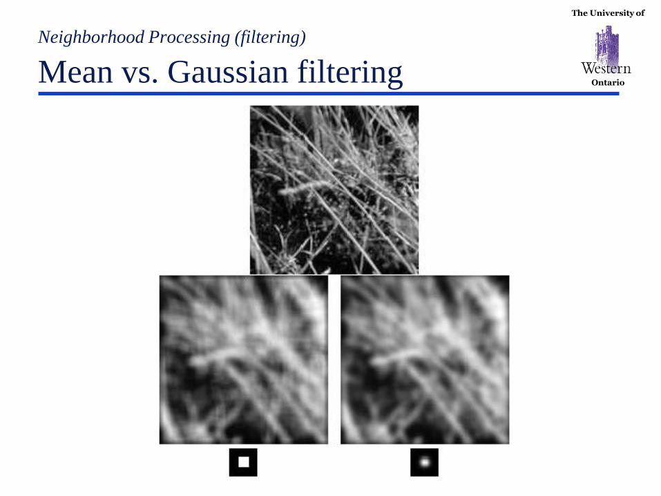
Mean kernel
What’s the kernel for a 3x3 mean filter?
0 0 0 0 0 0 0 0 0 0
0 0 0 0 0 0 0 0 0 0
0 0 0 90 90 90 90 90 0 0
0 0 0 90 90 90 90 90 0 0
0 0 0 90 90 90 90 90 0 0
0 0 0 90 0 90 90 90 0 0
0 0 0 90 90 90 90 90 0 0
0 0 0 0 0 0 0 0 0 0
0 0 90 0 0 0 0 0 0 0
0 0 0 0 0 0 0 0 0 0
],[ yxF
],[ vuH
The University of
Ontario
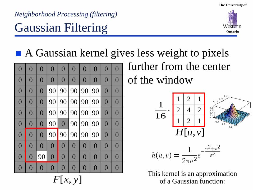
Neighborhood Processing (filtering)
Gaussian Filtering
A Gaussian kernel gives less weight to pixels
further from the center
of the window 0 0 0 0 0 0 0 0 0 0
0 0 0 0 0 0 0 0 0 0
0 0 0 90 90 90 90 90 0 0
0 0 0 90 90 90 90 90 0 0
0 0 0 90 90 90 90 90 0 0
0 0 0 90 0 90 90 90 0 0
0 0 0 90 90 90 90 90 0 0
0 0 0 0 0 0 0 0 0 0
0 0 90 0 0 0 0 0 0 0
0 0 0 0 0 0 0 0 0 0 This kernel is an approximation
of a Gaussian function:
1 2 1
2 4 2
1 2 1
],[ vuH
16
1
],[ yxF
The University of
Ontario
Neighborhood Processing (filtering)
Mean vs. Gaussian filtering
The University of
Ontario
Neighborhood Processing (filtering)
Median filters
A Median Filter operates over a window by
selecting the median intensity in the window.
What advantage does a median filter have over
a mean filter?
Is a median filter a kind of convolution?
- No, median filter is an example of non-linear filtering

The University of
Ontario
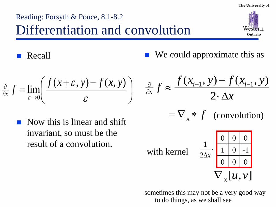
Reading: Forsyth & Ponce, 8.1-8.2
Differentiation and convolution
Recall
Now this is linear and shift
invariant, so must be the
result of a convolution.
We could approximate this as
(convolution)
with kernel
sometimes this may not be a very good way to do things, as we shall see
x
yxfyxff ii
x
2
),(),( 11
),(),(lim
0
yxfyxff
x
fx
0 0 0
1 0 -1
0 0 0
],[ vux
x2
1
The University of
Ontario
Reading: Forsyth & Ponce, 8.1-8.2
Differentiation and convolution
Recall
Now this is linear and shift
invariant, so must be the
result of a convolution.
We could approximate this as
(convolution)
with kernel
sometimes this may not be a very good way to do things, as we shall see
x
yxfyxff ii
x
2
),(),( 11
),(),(lim
0
yxfyxff
x
fx
0 0 0
1 0 -1
0 0 0
],[ vux
x2
1
The University of
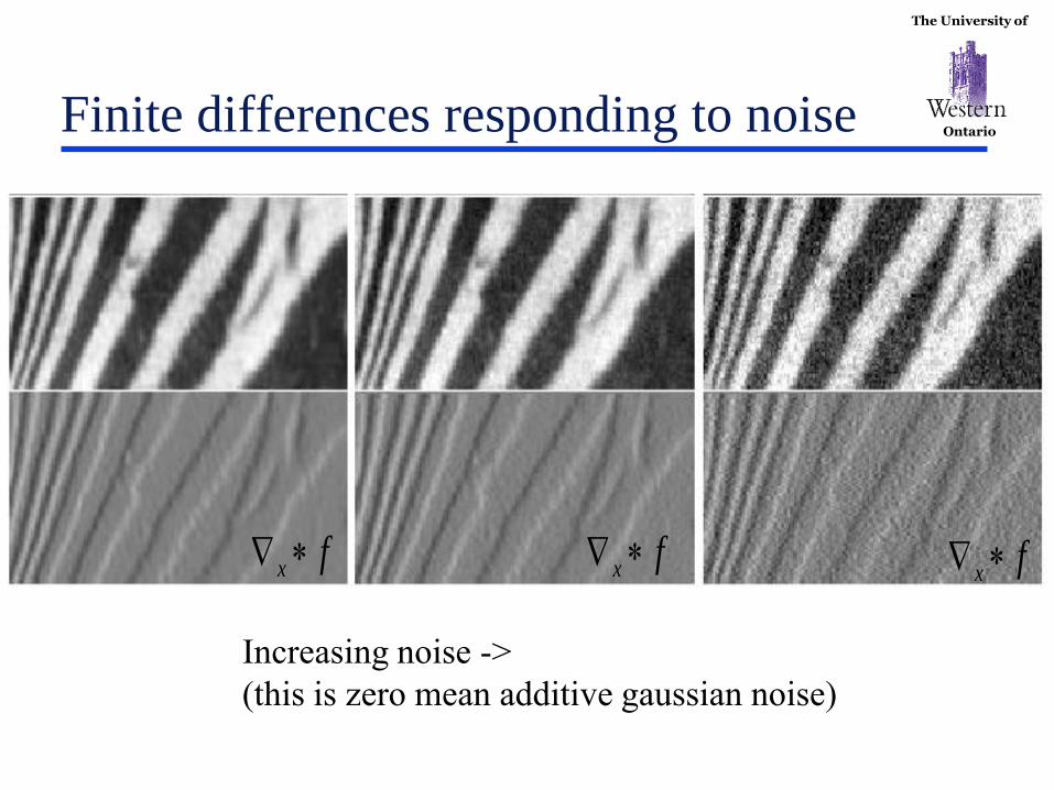
Ontario Finite differences responding to noise
Increasing noise ->
(this is zero mean additive gaussian noise)
fx fx fx
The University of
Ontario Finite differences and noise
Finite difference filters
respond strongly to noise
• obvious reason: image
noise results in pixels that
look very different from
their neighbours
Generally, the larger the
noise the stronger the
response
What is to be done?
• intuitively, most pixels in
images look quite a lot like
their neighbours
• this is true even at an edge;
along the edge they’re similar,
across the edge they’re not
• suggests that smoothing the
image should help, by forcing
pixels different to their
neighbours (=noise pixels?) to
look more like neighbours
The University of
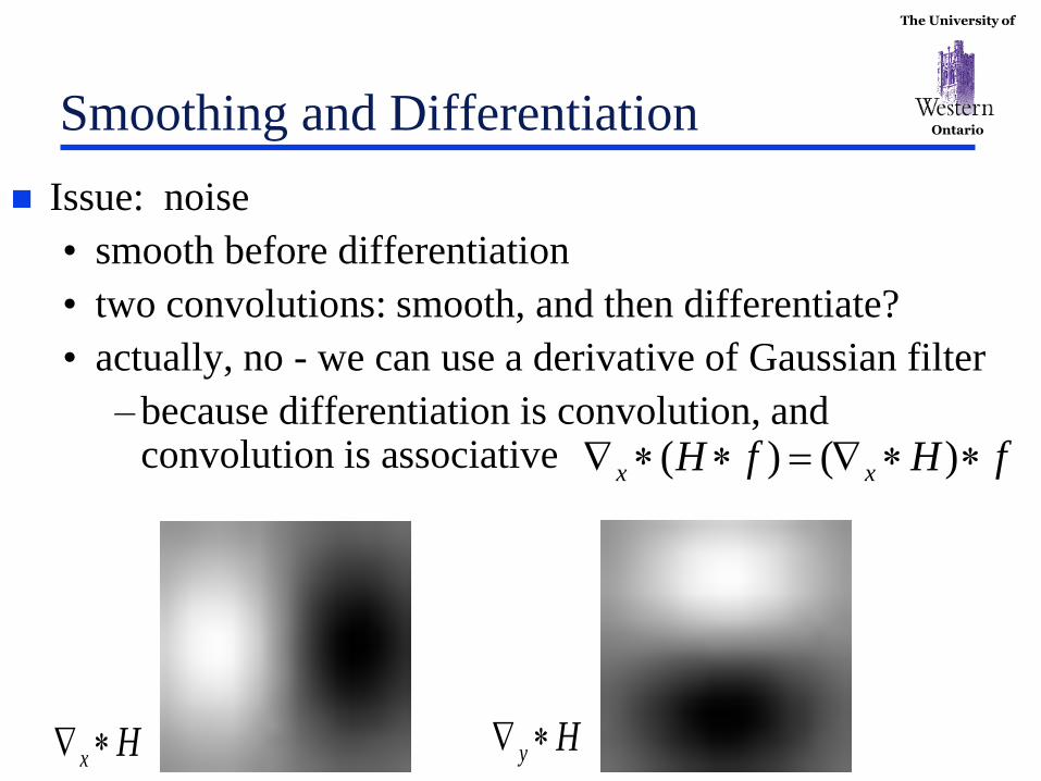
Ontario Smoothing and Differentiation
Issue: noise
• smooth before differentiation
• two convolutions: smooth, and then differentiate?
• actually, no - we can use a derivative of Gaussian filter
– because differentiation is convolution, and convolution is associative
Hx
fHfH xx )()(
Hy

The University of
Ontario
The scale of the smoothing filter affects derivative estimates, and also
the semantics of the edges recovered.
1 pixel 3 pixels 7 pixels
fHx )(
The University of
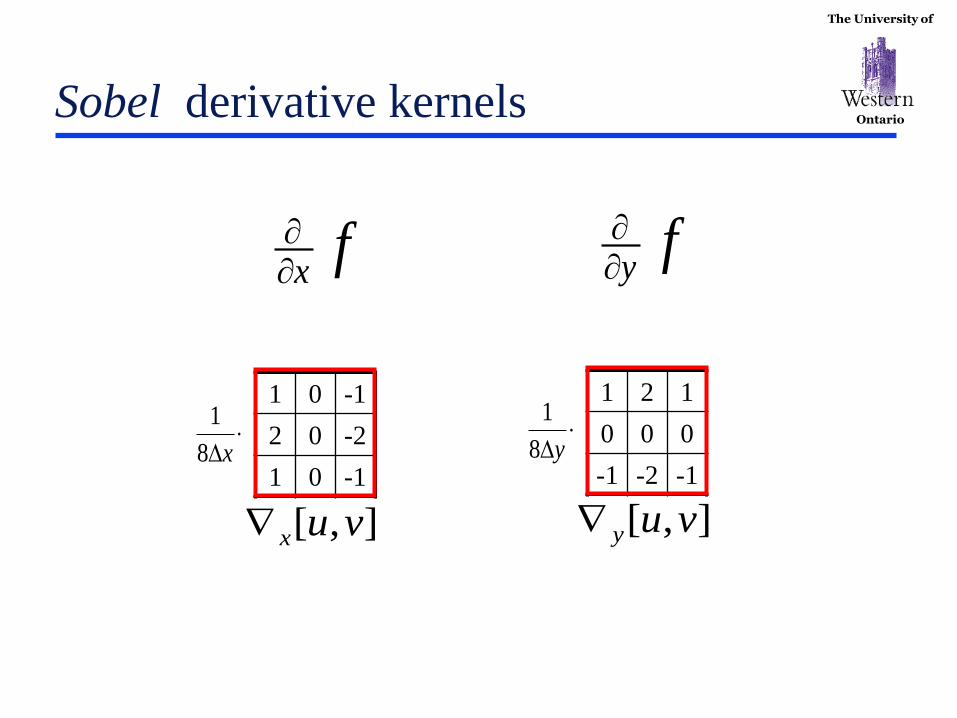
Ontario Sobel derivative kernels
1 0 -1
2 0 -2
1 0 -1
],[ vux
x8
1
fx
1 2 1
0 0 0
-1 -2 -1
],[ vuy
y8
1
fy
The University of
Ontario
x
f
y
f
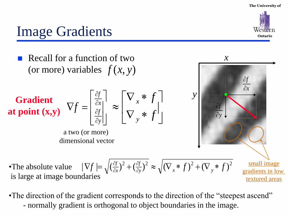
Image Gradients
Recall for a function of two
(or more) variables
f
f
y
x
y
f
x
f
f
),( yxf
Gradient
at point (x,y)
a two (or more)
dimensional vector
x
y
•The absolute value
is large at image boundaries
•The direction of the gradient corresponds to the direction of the “steepest ascend”
- normally gradient is orthogonal to object boundaries in the image.
2222 )()()()(|| fff yxy
f
x
f
small image
gradients in low
textured areas
The University of
Ontario
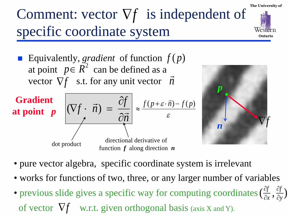
Comment: vector is independent of
specific coordinate system
n
fnf
)(
directional derivative of
function f along direction n
Equivalently, gradient of function
at point can be defined as a
vector s.t. for any unit vector
f
dot product
• pure vector algebra, specific coordinate system is irrelevant
• works for functions of two, three, or any larger number of variables
• previous slide gives a specific way for computing coordinates
of vector w.r.t. given orthogonal basis (axis X and Y).
2Rp )( pf
n
Gradient
at point p f
f
n
)()( pfnpf
p
f
),(y
f
x
f
The University of
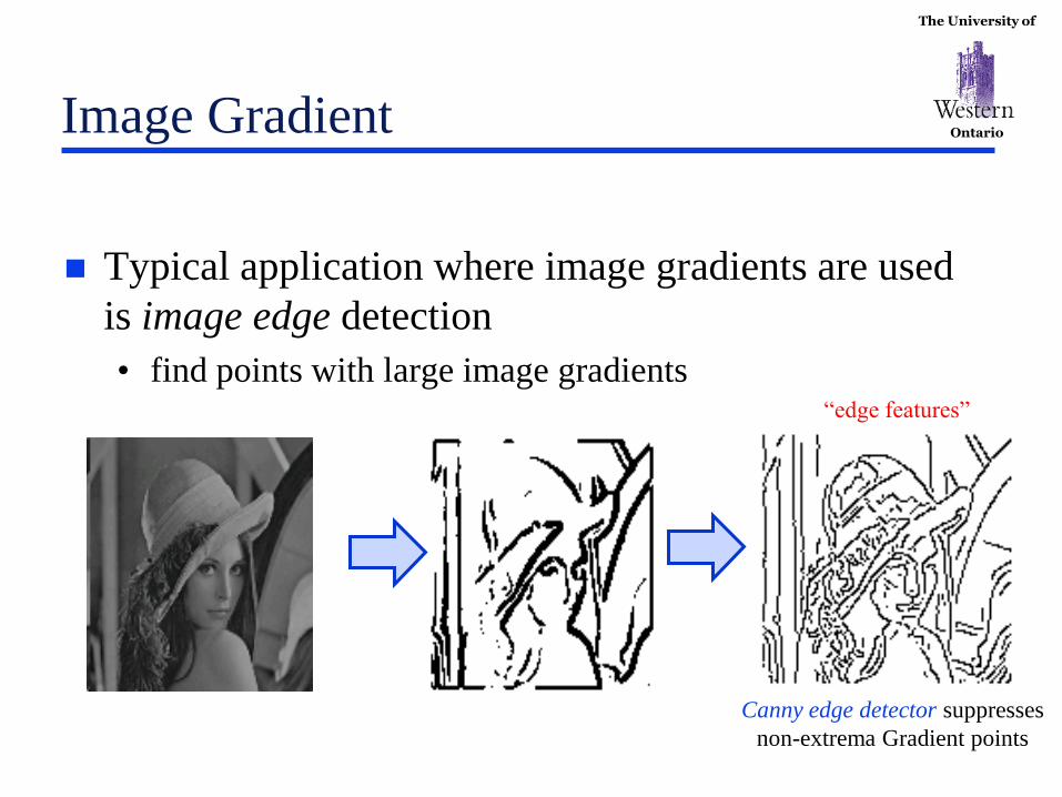
Ontario Image Gradient
Typical application where image gradients are used
is image edge detection
• find points with large image gradients
Canny edge detector suppresses
non-extrema Gradient points
“edge features”
The University of
Ontario
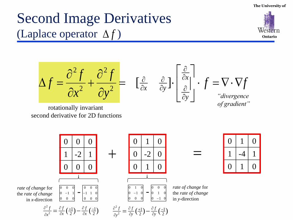
Second Image Derivatives (Laplace operator ) f
ffy
f
x
ff
y
x
yx
][
2
2
2
2
0 0 0
1 -2 1
0 0 0
0 1 0
0 -2 0
0 1 0
0 1 0
1 -4 1
0 1 0
“divergence
of gradient” rotationally invariant
second derivative for 2D functions
000
110
000
000
011
000
-
)()(21
21
2
2
x
f
x
f
x
f
rate of change for
the rate of change
in x-direction 000
010
010
010
010
000
-
)()(21
21
2
2
y
f
y
f
y
f
rate of change for
the rate of change
in y-direction
The University of
Ontario
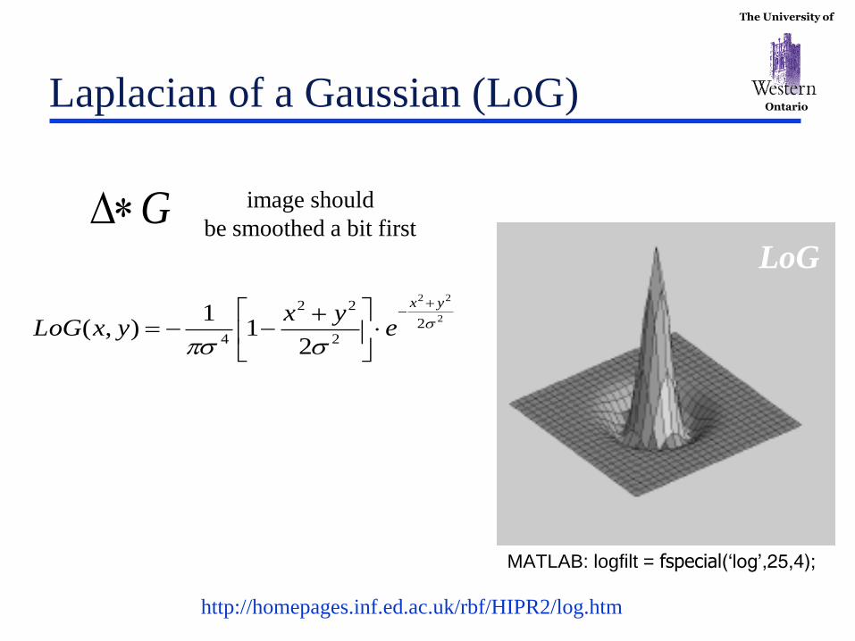
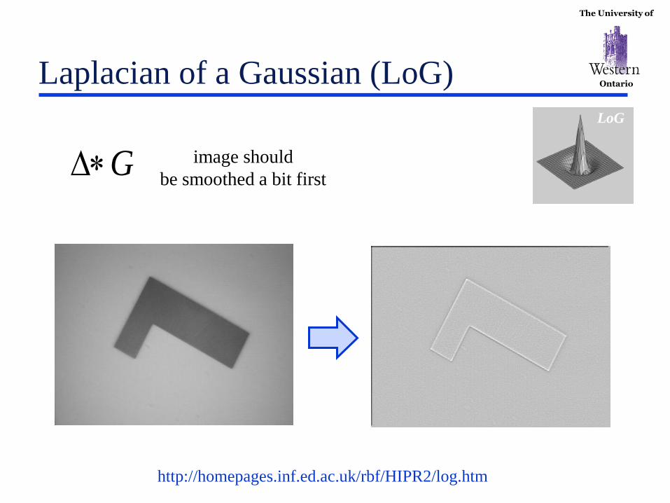
Laplacian of a Gaussian (LoG)
http://homepages.inf.ed.ac.uk/rbf/HIPR2/log.htm
MATLAB: logfilt = fspecial(‘log’,25,4);
2
22
22
22
4 21
1),(
yx
eyx
yxLoG
LoG
G image should
be smoothed a bit first
The University of
Ontario
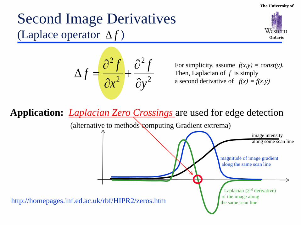
Second Image Derivatives (Laplace operator )
magnitude of image gradient
along the same scan line
Application: Laplacian Zero Crossings are used for edge detection
(alternative to methods computing Gradient extrema)
http://homepages.inf.ed.ac.uk/rbf/HIPR2/zeros.htm
image intensity
along some scan line
Laplacian (2nd derivative)
of the image along
the same scan line
f
2
2
2
2
y
f
x
ff
For simplicity, assume f(x,y) = const(y).
Then, Laplacian of f is simply
a second derivative of f(x) = f(x,y)
The University of
Ontario
Laplacian of a Gaussian (LoG)
G image should
be smoothed a bit first
LoG
http://homepages.inf.ed.ac.uk/rbf/HIPR2/log.htm
The University of
Ontario
+a = ?
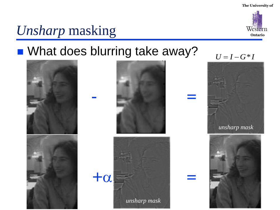
Unsharp masking
What does blurring take away?
- =
unsharp mask
unsharp mask
IGIU *
The University of
Ontario
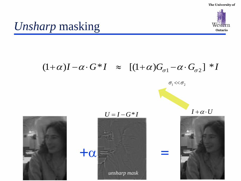
+a = ?
Unsharp masking
unsharp mask
unsharp mask
IGIU * UI a
IGGIGI *])1[(*)1( 21 aaaa
21
The University of
Ontario
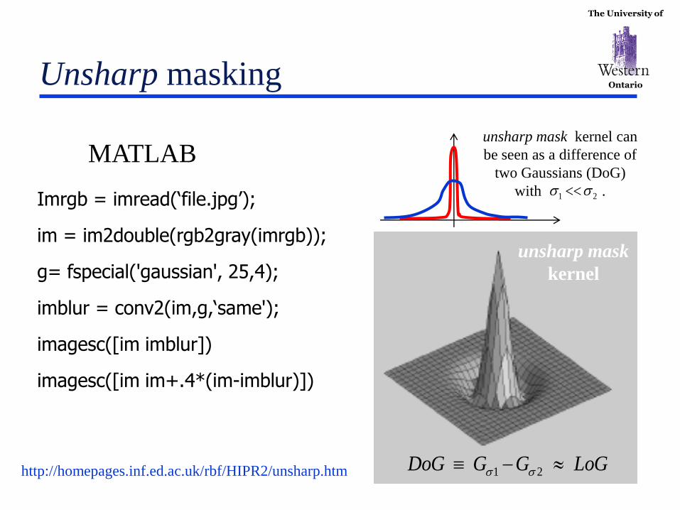
Unsharp masking
MATLAB
Imrgb = imread(‘file.jpg’);
im = im2double(rgb2gray(imrgb));
g= fspecial('gaussian', 25,4);
imblur = conv2(im,g,‘same');
imagesc([im imblur])
imagesc([im im+.4*(im-imblur)])
unsharp mask kernel can
be seen as a difference of
two Gaussians (DoG)
with .
LoGGGDoG 21
21
unsharp mask
kernel
http://homepages.inf.ed.ac.uk/rbf/HIPR2/unsharp.htm
The University of
Ontario
Reading: Forsyth & Ponce ch.7.5
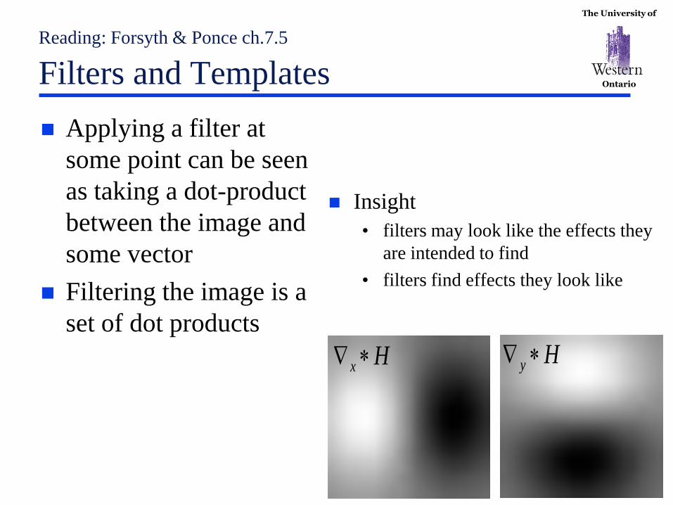
Filters and Templates
Applying a filter at
some point can be seen
as taking a dot-product
between the image and
some vector
Filtering the image is a
set of dot products
Insight
• filters may look like the effects they
are intended to find
• filters find effects they look like
Hx Hy
The University of
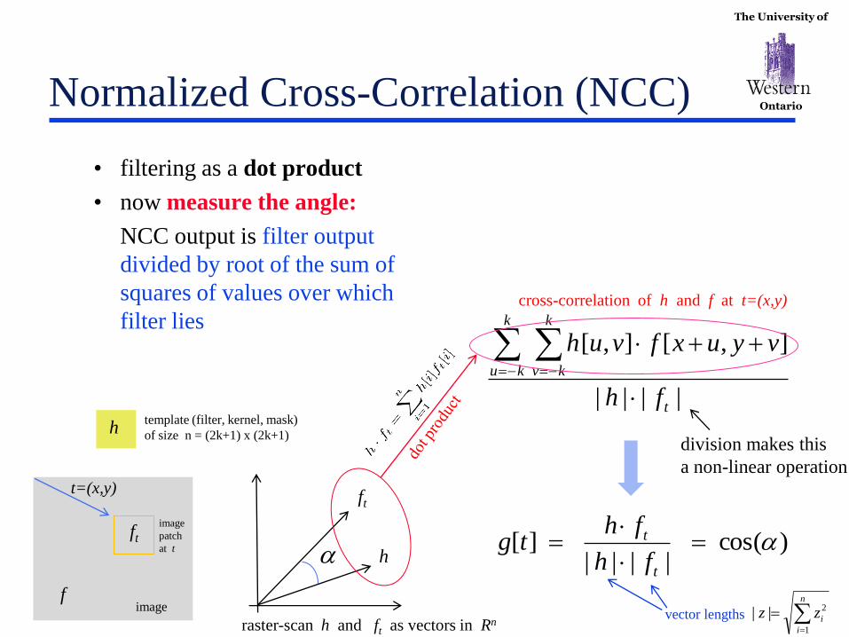
Ontario Normalized Cross-Correlation (NCC)
• filtering as a dot product
• now measure the angle:
NCC output is filter output
divided by root of the sum of
squares of values over which
filter lies
||||
],[],[
t
k
ku
k
kv
fh
vyuxfvuh
cross-correlation of h and f at t=(x,y)
division makes this
a non-linear operation
)cos(||||
][ a
t
t
fh
fhtg
a h
ft
raster-scan h and ft as vectors in Rn
f
t=(x,y)
ft
h
image
template (filter, kernel, mask)
of size n = (2k+1) x (2k+1)
image
patch
at t
n
i
izz1
2||vector lengths
The University of
Ontario Normalized Cross-Correlation (NCC)
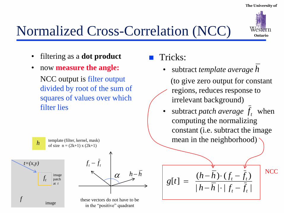
Tricks:
• subtract template average
(to give zero output for constant
regions, reduces response to
irrelevant background)
• subtract patch average when
computing the normalizing
constant (i.e. subtract the image
mean in the neighborhood)
f
t=(x,y)
ft
h
image
||||
)()(][
tt
tt
ffhh
ffhhtg
• filtering as a dot product
• now measure the angle:
NCC output is filter output
divided by root of the sum of
squares of values over which
filter lies
a hh
tt ff
these vectors do not have to be
in the “positive” quadrant
image
patch
at t
NCC
h
tf
template (filter, kernel, mask)
of size n = (2k+1) x (2k+1)
The University of
Ontario Normalized Cross-Correlation (NCC)
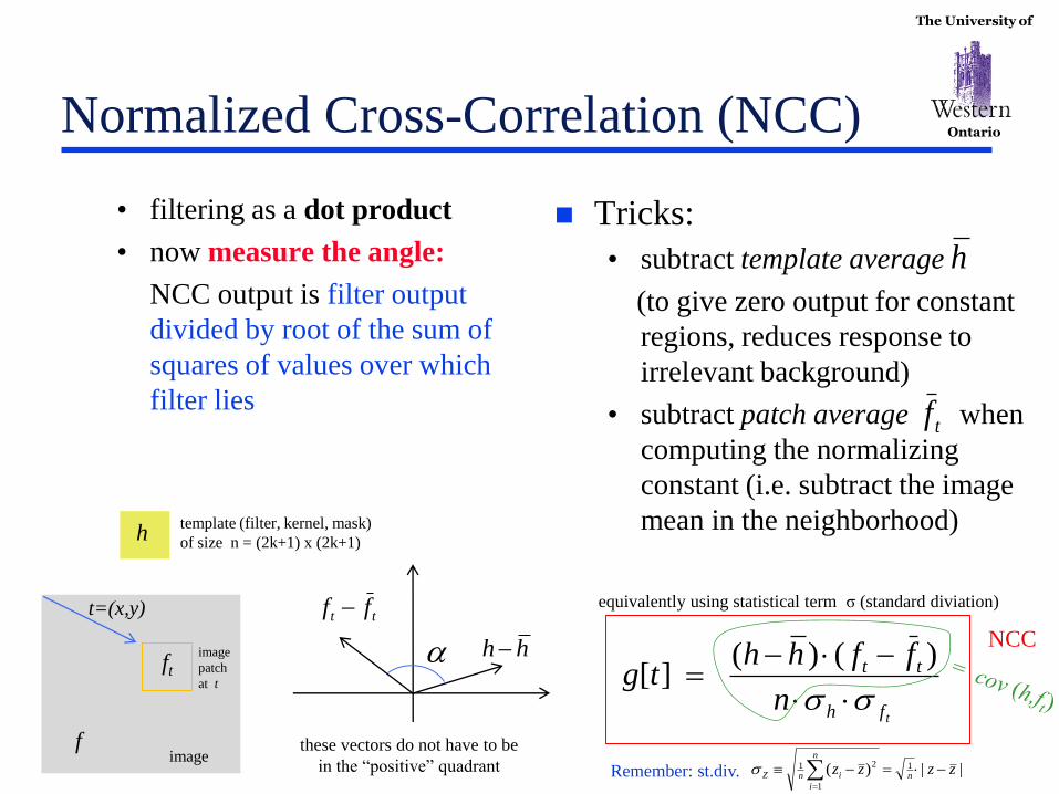
Tricks:
• subtract template average
(to give zero output for constant
regions, reduces response to
irrelevant background)
• subtract patch average when
computing the normalizing
constant (i.e. subtract the image
mean in the neighborhood)
f
t=(x,y)
ft
h
image
• filtering as a dot product
• now measure the angle:
NCC output is filter output
divided by root of the sum of
squares of values over which
filter lies
a hh
tt ff
these vectors do not have to be
in the “positive” quadrant
image
patch
at t
NCC
h
tf
tfh
tt
n
ffhhtg
)()(][
equivalently using statistical term σ (standard diviation)
||)( 1
1
21 zzzzn
n
i
inZ
Remember: st.div.
template (filter, kernel, mask)
of size n = (2k+1) x (2k+1)

The University of
Ontario Normalized Cross-Correlation (NCC)
f
t=(x,y)
ft
h
image
tfh
tfhtg
),cov(][
standard in statistics
correlation coefficient
between h and ft
• filtering as a dot product
• now measure the angle:
NCC output is filter output
divided by root of the sum of
squares of values over which
filter lies
NCC
equivalently using statistical term cov (covariance)
image
patch
at t
n
bbaabbaabbaaEba
n
i
iin
)()())(())((),cov(
1
1
Tricks:
• subtract template average
(to give zero output for constant
regions, reduces response to
irrelevant background)
• subtract patch average when
computing the normalizing
constant (i.e. subtract the image
mean in the neighborhood)
h
tf
template (filter, kernel, mask)
of size n = (2k+1) x (2k+1)

The University of
Ontario
hA hB hC hD
Normalized Cross-Correlation (NCC)
NCC for h and f
image f A
B
C
D
points mark local maxima of NCC
for each template
C
templates
points of interest or feature points
pictures from Silvio Savarese
The University of
Ontario Other features… (Szeliski sec 4.1.1)
Feature points are used for:
• Image alignment (homography, fundamental matrix)
• 3D reconstruction
• Motion tracking
• Object recognition
• Indexing and database retrieval
• Robot navigation
• … other
The University of
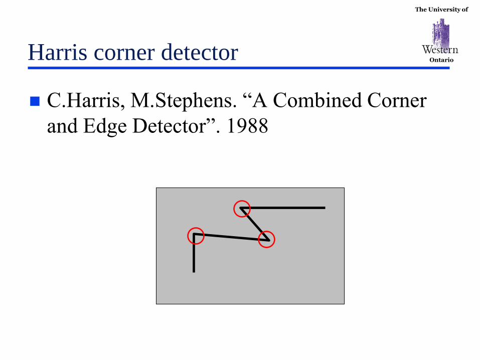
Ontario Harris corner detector
C.Harris, M.Stephens. “A Combined Corner
and Edge Detector”. 1988

The University of
Ontario
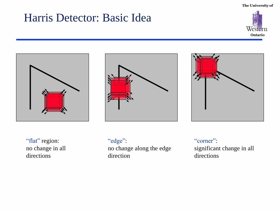
The Basic Idea
We should easily recognize the point by looking through a small window
Shifting a window in any direction should give a large change in intensity
The University of
Ontario
Harris Detector: Basic Idea
“flat” region:
no change in all
directions
“edge”:
no change along the edge
direction
“corner”:
significant change in all
directions
The University of
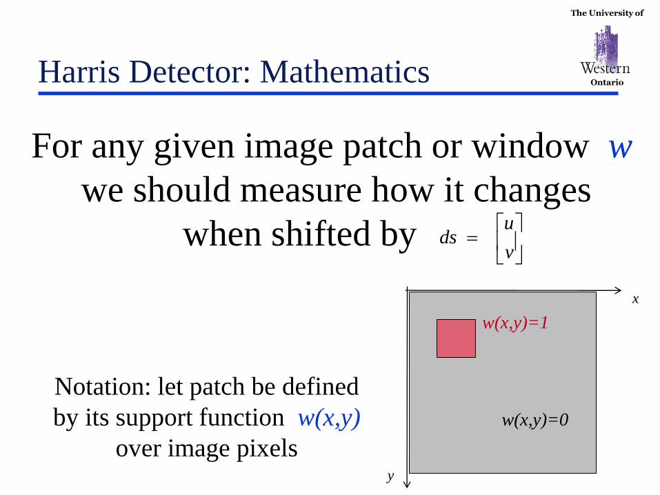
Ontario Harris Detector: Mathematics
For any given image patch or window w
we should measure how it changes
when shifted by
Notation: let patch be defined
by its support function w(x,y)
over image pixels
x
y
w(x,y)=0
w(x,y)=1
v
uds
The University of
Ontario
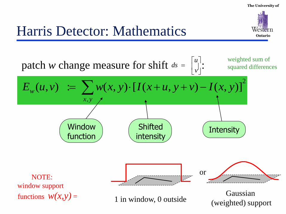
2
,
)],(),([),(:),( yx
w yxIvyuxIyxwvuE
Harris Detector: Mathematics
patch w change measure for shift :
Intensity Shifted intensity
Window function
or NOTE:
window support
functions w(x,y) = Gaussian
(weighted) support 1 in window, 0 outside
weighted sum of
squared differences
v
uds
The University of
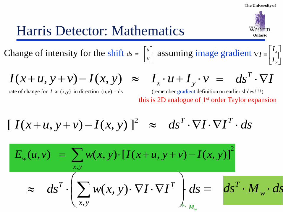
Ontario Harris Detector: Mathematics
vIuIyxIvyuxI yx ),(),(
dsIIdsyxIvyuxI TT 2]),(),([
IdsT
dsIIyxwds T
yx
T
,
),(
2
,
)],(),([),(),( yx
w yxIvyuxIyxwvuE
Change of intensity for the shift assuming image gradient
v
uds
y
x
I
II
rate of change for I at (x,y) in direction (u,v) = ds (remember gradient definition on earlier slides!!!!)
this is 2D analogue of 1st order Taylor expansion
dsMds w
T
Mw
The University of
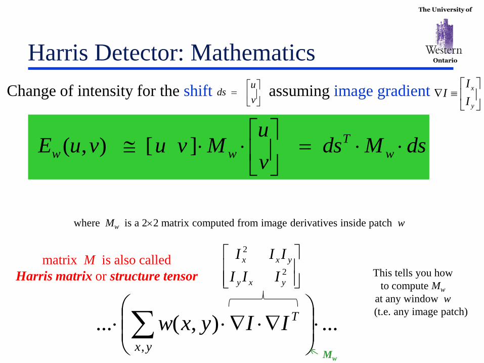
Ontario Harris Detector: Mathematics
dsMdsv
uMvuvuE w
T
ww
][),(
Change of intensity for the shift assuming image gradient
v
uds
y
x
I
II
...),(...,
T
yx
IIyxw
Mw
where Mw is a 22 matrix computed from image derivatives inside patch w
2
2
yxy
yxx
III
III
This tells you how
to compute Mw
at any window w
(t.e. any image patch)
matrix M is also called
Harris matrix or structure tensor
The University of
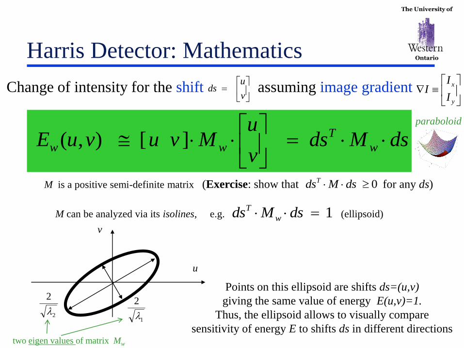
Ontario Harris Detector: Mathematics
M is a positive semi-definite matrix (Exercise: show that for any ds) 0 dsMdsT
M can be analyzed via its isolines, e.g. (ellipsoid) 1 dsMds w
T
Points on this ellipsoid are shifts ds=(u,v)
giving the same value of energy E(u,v)=1.
Thus, the ellipsoid allows to visually compare
sensitivity of energy E to shifts ds in different directions
u
v
1
2
2
2
dsMdsv
uMvuvuE w
T
ww
][),(
Change of intensity for the shift assuming image gradient
v
uds
y
x
I
II
paraboloid
two eigen values of matrix Mw
The University of
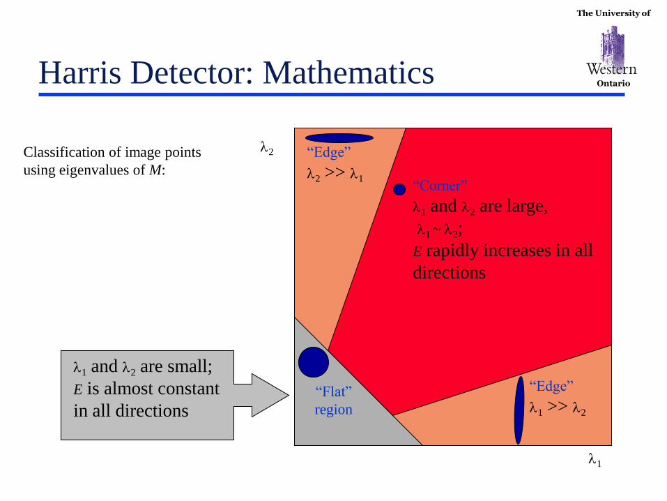
Ontario Harris Detector: Mathematics
1
2
“Corner”
1 and 2 are large,
1 ~ 2;
E rapidly increases in all
directions
1 and 2 are small;
E is almost constant
in all directions
“Edge”
1 >> 2
“Edge”
2 >> 1
“Flat”
region
Classification of image points
using eigenvalues of M:
The University of
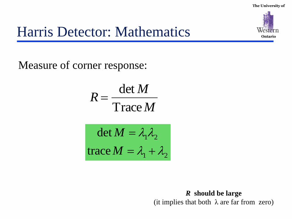
Ontario Harris Detector: Mathematics
Measure of corner response:
1 2
1 2
det
trace
M
M
M
MR
Trace
det
R should be large
(it implies that both λ are far from zero)
The University of
Ontario Harris Detector
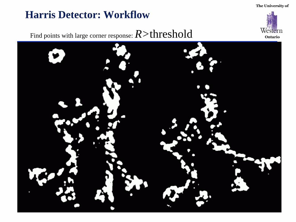
The Algorithm:
• Find points with large corner response function R
R > threshold
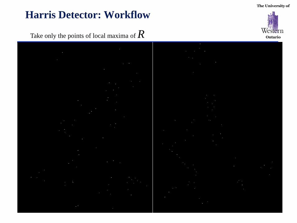
• Take the points of local maxima of R

The University of
Ontario
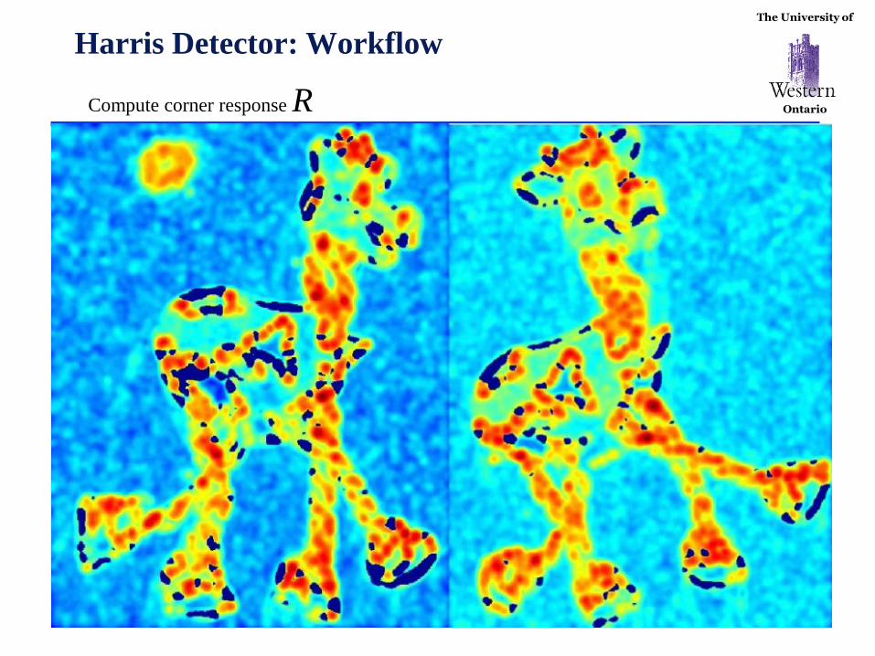
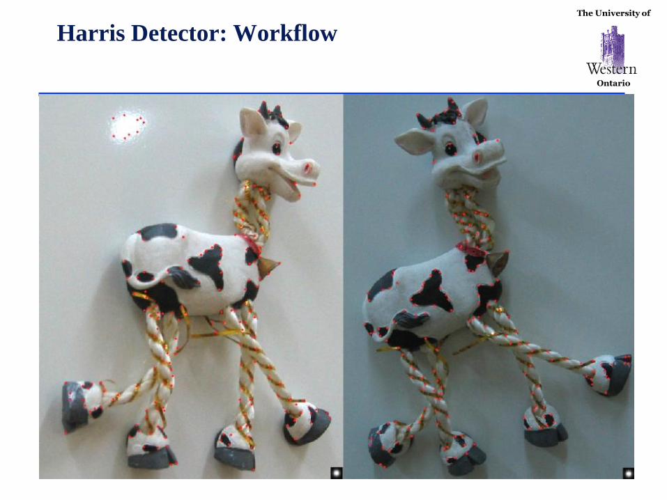
Harris Detector: Workflow
Find points with large corner response: R>threshold
The University of
Ontario
Harris Detector: Workflow
Take only the points of local maxima of R
The University of
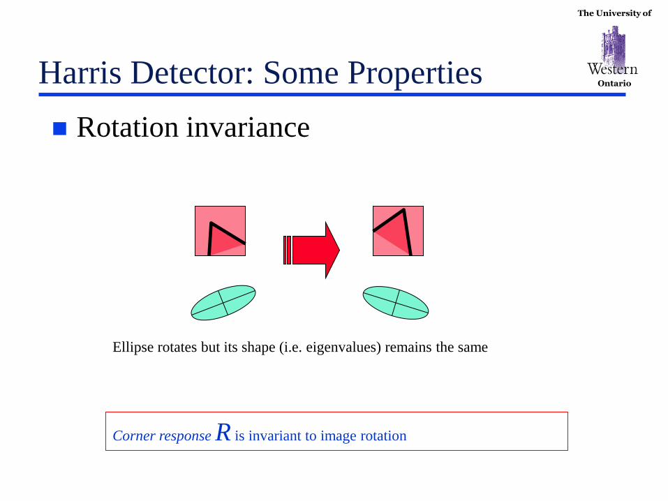
Ontario Harris Detector: Some Properties
Rotation invariance
Ellipse rotates but its shape (i.e. eigenvalues) remains the same
Corner response R is invariant to image rotation
The University of
Ontario Harris Detector: Some Properties
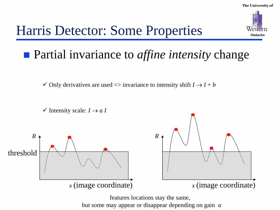
Partial invariance to affine intensity change
Only derivatives are used => invariance to intensity shift I I + b
Intensity scale: I a I
R
x (image coordinate)
threshold
R
x (image coordinate)
features locations stay the same,
but some may appear or disappear depending on gain a
The University of
Ontario Harris Detector: Some Properties
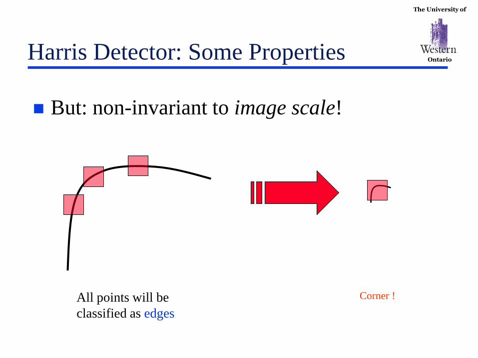
But: non-invariant to image scale!
All points will be
classified as edges
Corner !
The University of
Ontario Scale Invariant Detection
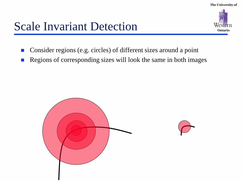
Consider regions (e.g. circles) of different sizes around a point
Regions of corresponding sizes will look the same in both images
The University of
Ontario Scale Invariant Detection
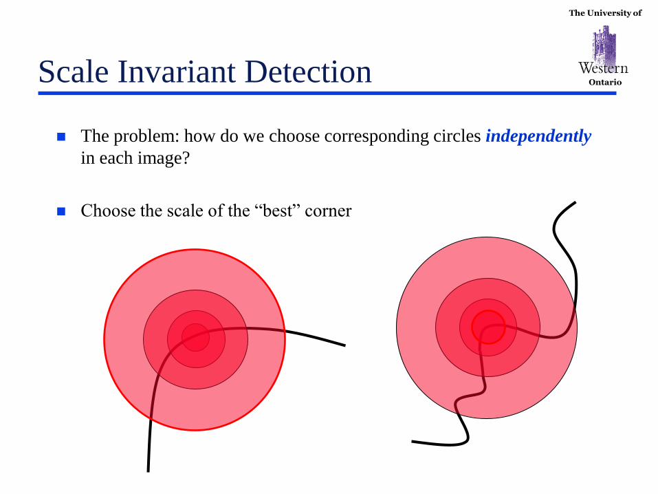
The problem: how do we choose corresponding circles independently
in each image?
Choose the scale of the “best” corner
The University of
Ontario Other feature detectors
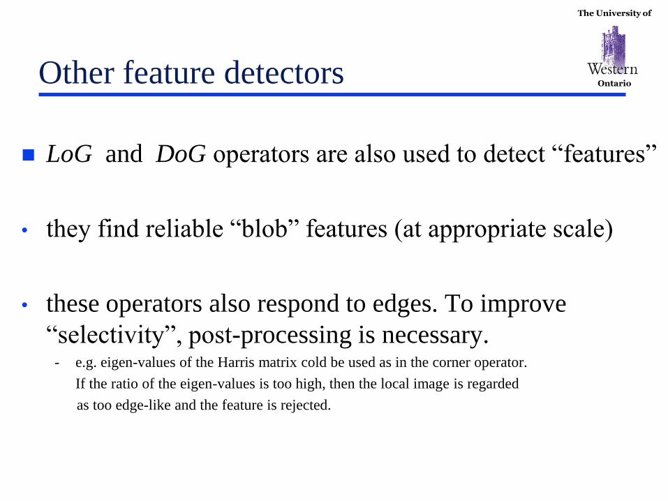
LoG and DoG operators are also used to detect “features”
• they find reliable “blob” features (at appropriate scale)
• these operators also respond to edges. To improve
“selectivity”, post-processing is necessary. - e.g. eigen-values of the Harris matrix cold be used as in the corner operator.
If the ratio of the eigen-values is too high, then the local image is regarded
as too edge-like and the feature is rejected.
The University of
Ontario Other features
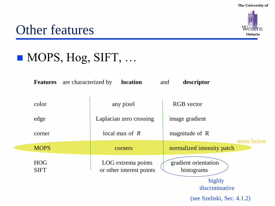
MOPS, Hog, SIFT, …
Features are characterized by location and descriptor
color any pixel RGB vector
edge Laplacian zero crossing image gradient
corner local max of R magnitude of R
MOPS corners normalized intensity patch
HOG LOG extrema points gradient orientation
SIFT or other interest points histograms
highly
discriminative
(see Szeliski, Sec. 4.1.2)
more below
The University of
Ontario Feature descriptors
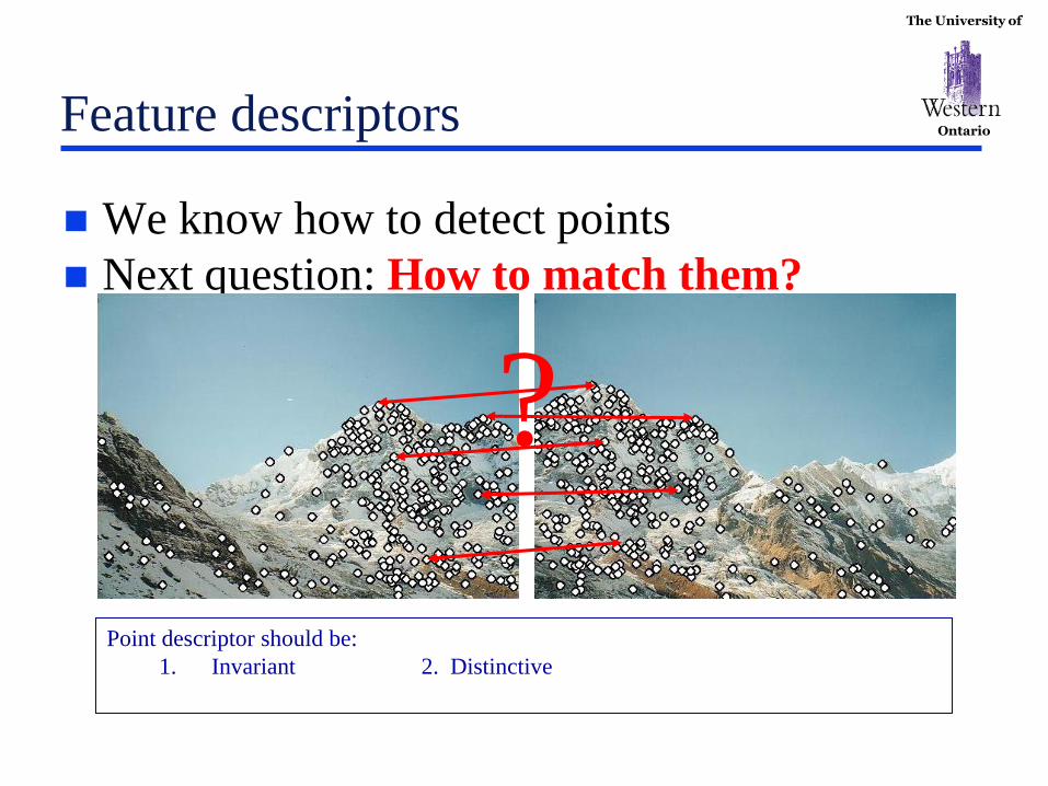
We know how to detect points
Next question: How to match them?
?
Point descriptor should be:
1. Invariant 2. Distinctive
The University of
Ontario
Descriptors Invariant to Rotation
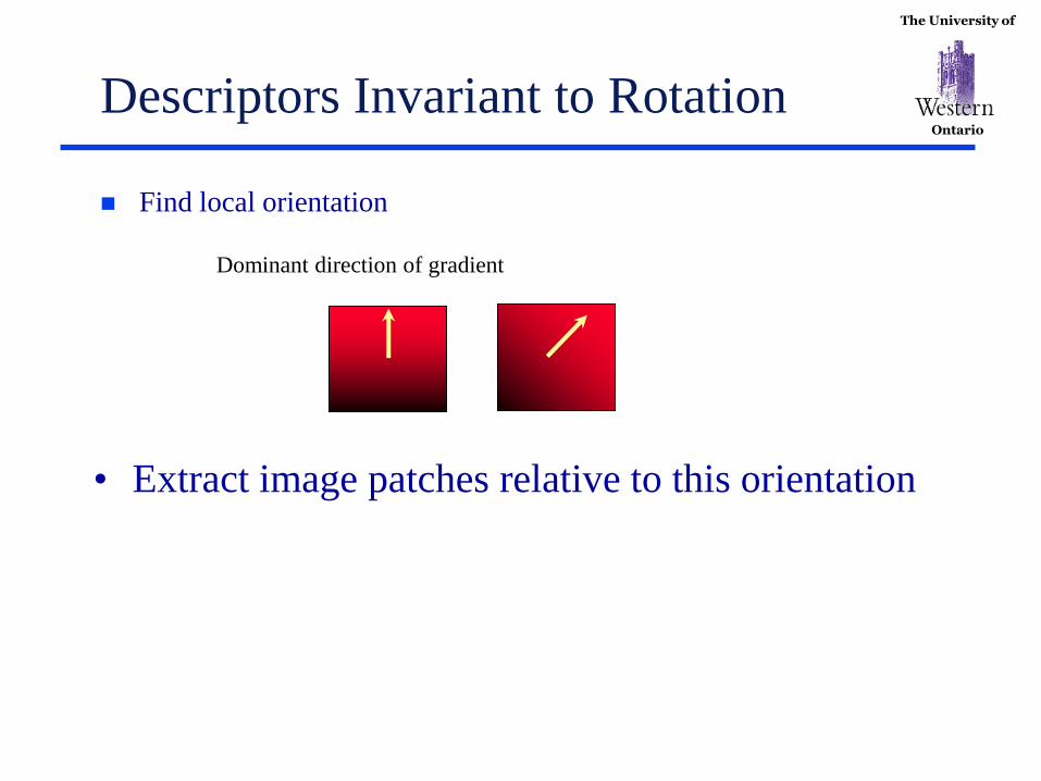
Find local orientation
Dominant direction of gradient
• Extract image patches relative to this orientation

The University of
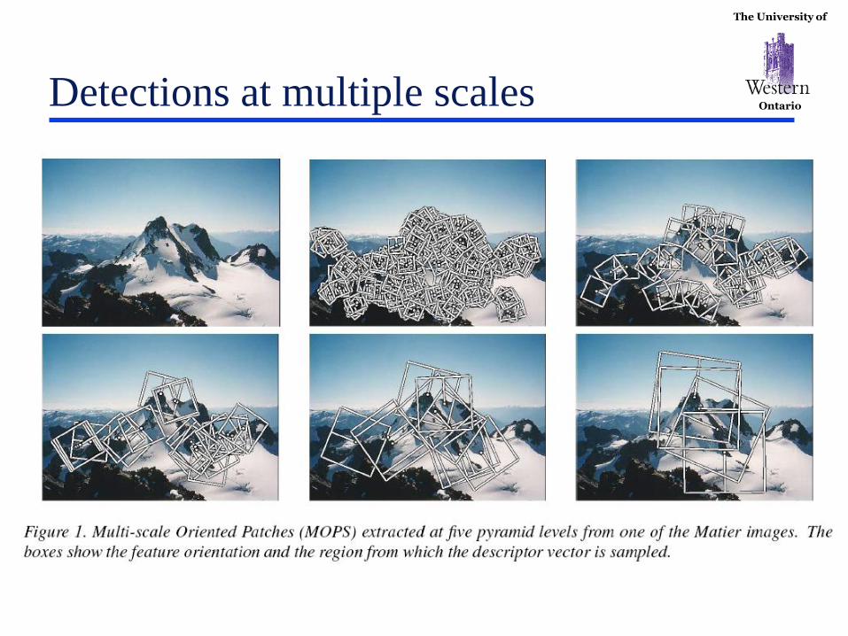
Ontario Multi-Scale Oriented Patches (MOPS)
Interest points
• Multi-scale Harris corners
• Orientation from blurred gradient
• Geometrically invariant to rotation
Descriptor vector
• Bias/gain normalized sampling of local patch (8x8)
• Photometrically invariant to affine changes in intensity
[Brown, Szeliski, Winder, CVPR’2005]
The University of
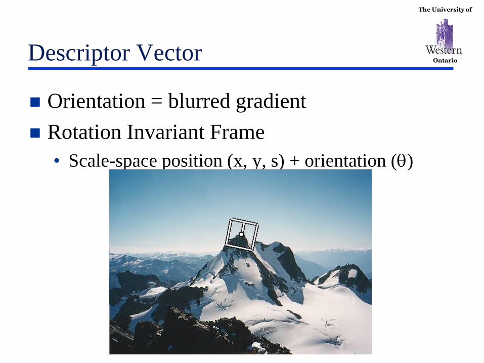
Ontario Descriptor Vector
Orientation = blurred gradient
Rotation Invariant Frame
• Scale-space position (x, y, s) + orientation ()
The University of
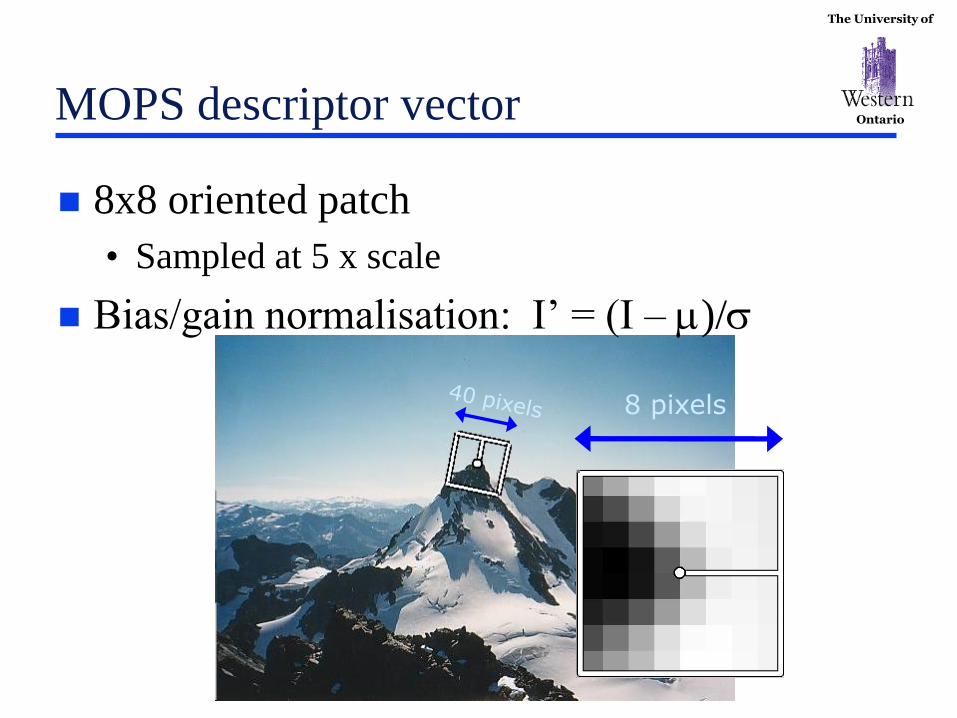
Ontario MOPS descriptor vector
8x8 oriented patch
• Sampled at 5 x scale
Bias/gain normalisation: I’ = (I – )/
8 pixels