The University of

Ontario

The University of

Ontario

5-1

CS 4487/9587

Algorithms for Image Analysis

2D Segmentation (part II)

Deformable Models

Acknowledgements: many slides from the University of Manchester, demos from Visual Dynamics Group (University

of Oxford),

The University of

Ontario

The University of

Ontario

5-2

CS 4487/9587 Algorithms for Image Analysis Deformable Models in 2D

Active Contours or “snakes” • “snakes” vs. “livewire”• (discrete) energy formulations for snakes• relation to Hidden Markov Models (HMM)

Optimization (discrete case)• Gradient Descent• Dynamic Programming (DP), Viterbi algorithm• DP versus Dijkstra

Extra Reading: Sonka et.al 5.2.5 and 8.2 Active Contours by Blake and

Isard

The University of

Ontario

The University of

Ontario

5-3

“Live-wire” vs. “Snakes”

• intelligent scissors [Mortensen, Barrett 1995]

• live-wire [Falcao, Udupa, Samarasekera, Sharma 1998]

1

23

4

Shortest paths on image-based graph connect seeds placed on object boundary

The University of

Ontario

The University of

Ontario

5-4

“Live-wire” vs. “Snakes”

Given: initial contour (model) near desirable object

• Snakes, active contours [Kass, Witkin, Terzopoulos 1987]

• In general, deformable models are widely used

The University of

Ontario

The University of

Ontario

5-5

“Live-wire” vs. “Snakes”

• Snakes, active contours [Kass, Witkin, Terzopoulos 1987]

• In general, deformable models are widely used

Given: initial contour (model) near desirable object

Goal: evolve the contour to fit exact object boundary

The University of

Ontario

The University of

Ontario

5-6

Tracking via deformable models

1. Use final contour/model extracted at frame t as an initial solution for frame t+1

2. Evolve initial contour to fit exact object boundary at frame t+1

3. Repeat steps 1 and 2 for t ‘= t+1

The University of

Ontario

The University of

Ontario

5-7

Tracking via deformable models

Acknowledgements: Visual Dynamics Group, Dept. Engineering Science, University of Oxford.

Traffic monitoringHuman-computer interactionAnimationSurveillanceComputer Assisted Diagnosis in medical imaging

Applications:

The University of

Ontario

The University of

Ontario

5-8

Tracking via deformable models

Tracking Heart Ventricles

The University of

Ontario

The University of

Ontario

5-9

“Snakes”

A smooth 2D curve which matches to image data Initialized near target, iteratively refined Can restore missing data

initial intermediate final

Q: How does that work? ….

gradient descent w.r.t. some function describing snake’s quality

The University of

Ontario

The University of

Ontario

5-10

Preview

assume some energy function f(x) describing snake’s “quality” f(x)

0x

)x('ftxx ii1i

gradient descent for 1D functions

1x2x

local minima for f(x)

x̂

1Rx

for simplicity, assume that "snake” is a vector (or point) in R1

Q: Is snake (contour) a point in some space? ... Yes

The University of

Ontario

The University of

Ontario

5-11

Parametric Curve Representation(continuous case)

A curve can be represented by 2 functions

open curve closed curve

1s0))s(y),s(x()s( ν

Note: in computer vision and medical imaging the term “snake” is commonly associated with such parametric representation of contours. (Other representations will be discussed later!)

Here, contour is a point in (space of functions) R]}1,0[s|)s({ νC

parameter

The University of

Ontario

The University of

Ontario

5-12

Parametric Curve Representation(discrete case)

A curve can be represented by a set of 2D points

niyx iii 0),(ν

Here, contour is a point in _ n2R

)y,x,....,y,x,y,x()ni0|( 1n1n1100i νC

),( nn yx

parameter

The University of

Ontario

The University of

Ontario

5-13

Measuring snake’s quality: Energy function

Contours can be seen as points C in (or in )

We can define some energy function E(C) that assigns some number (quality measure) to all possible snakes

n2R R

)y,x,....,y,x,y,x(),....,,,( 1n1n11001n210 ννννC

E(C)RR n2

(scalars)(contours C)

Q: Did we use any function (energy) to measure quality of segmentation results in 1) image thresholding? 2) region growing? 3) live-wire?

NO

NO

YES (will compare later)

WHY?: Somewhat philosophical question,

but specifying a quality function E(C) is an

objective way to define what “good” means

for contours C.

Moreover, one can find “the best”

contour (segmentation) by optimizing

energy E(C).

The University of

Ontario

The University of

Ontario

5-14

Energy function

Usually, the total energy of snake is a combination of internal and external energies

exin EEE

Internal energy encourages smoothness or any particular

shape

Internal energy incorporates prior knowledge about object boundary

allowing to extract boundary even if some image data is

missing

External energy encourages curve onto image structures (e.g. image

edges)

The University of

Ontario

The University of

Ontario

5-15

Internal Energy (continuous case)

The smoothness energy at contour point v(s) could be evaluated as

Then, the interior energy (smoothness) of the whole snake is

Elasticity/stretching Stiffness/bending

sd

ddsd

sssEin 2

2

)()())((

22

1

0

inin ds))s((EE ]}1,0[s|)s({ νC

The University of

Ontario

The University of

Ontario

Internal Energy(discrete case)

5v4v

3v

2v

1v6v

7v

8v

10v

9v

elastic energy(elasticity)

i1ivds

d

bending energy(stiffness)

1ii1i1iii1i2

2

2)()(ds

d

)( iii y,xν

2n)( 1n210 ,....,,, ννννC

The University of

Ontario

The University of

Ontario

5-17

Internal Energy(discrete case)

Elasticity Stiffness

i1ivds

d

11112

2

2)()( iiiiiiids

d

1

0

211

21 |2|||

n

iiiiiiinE

)( iii y,xν

2n)( 1n210 ,....,,, ννννC

The University of

Ontario

The University of

Ontario

5-18

External energy

The external energy describes how well the curve matches the image data locally

Numerous forms can be used, attracting the curve toward different image features

The University of

Ontario

The University of

Ontario

5-19

External energy

Suppose we have an image I(x,y) Can compute image gradient at any point Edge strength at pixel (x,y) is External energy of a contour point v=(x,y) could be

)I,I(I yx|)y,x(I|

22 |),(||)(|)( yxIIEex vv

1

0

)(n

iiexex EE discrete case

}ni0|{ i νC

1

0

))(( dssEE exex continuous case ]}1,0[s|)s({ νC

External energy term for the whole snake is

The University of

Ontario

The University of

Ontario

5-20

Basic Elastic Snake

The total energy of a basic elastic snake is

continuous case

discrete case

1

0

21

0

2 ds|))s(v(I|ds|ds

dv|E

1n

0i

2i

1n

0i

2i1i |)v(I||vv|E

elastic smoothness term(interior energy)

image data term(exterior energy)

]}1,0[s|)s({ νC

}ni0|{ i νC

The University of

Ontario

The University of

Ontario

5-21

Basic Elastic Snake(discrete case)

This can make a curve shrink

(to a point)

1

0

2n

iiin LE

21

1

0

21 )()( ii

n

iii yyxx

1n

0i

2iiex |)y,x(I|E

21

0

2 |),(||),(| iiy

n

iiix yxIyxI

)y,x,....,y,x,y,x()ni0|( 1n1n1100i νC

C

ii-1 i+1

i+2

Li-1 Li

Li+1

The University of

Ontario

The University of

Ontario

5-22

Basic Elastic Snake (discrete case)

The problem is to find contour

that minimizes

Optimization problem for function of 2n variables• can compute local minima via gradient descent (coming soon)

• potentially more robust option: dynamic programming (later)

2iiy

1n

0i

2iix

2i1i

1n

0i

2i1i |)y,x(I||)y,x(I|)yy()xx()(E

C

nnn Ryyxx 2

1010 ),,,,,( C

The University of

Ontario

The University of

Ontario

5-23

Basic Elastic Snake

Synthetic example

(1) (2)

(3) (4)

The University of

Ontario

The University of

Ontario

5-24

Basic Elastic Snake

Dealing with missing data

The smoothness constraint can deal with missing data:

The University of

Ontario

The University of

Ontario

5-25

Basic Elastic Snake

Relative weighting

Notice that the strength of the internal elastic component can be controlled by a parameter,

Increasing this increases stiffness of curve

large small medium

1

0

2n

iiin LE

The University of

Ontario

The University of

Ontario

5-26

Encouraging point spacing

To stop the curve from shrinking to a point

• encourages particular point separation

1

0

2)ˆ(n

iiiin LLE

The University of

Ontario

The University of

Ontario

5-27

Simple shape prior

If object is some smooth variation on a known shape, use

– where give points of the basic shape

1

0

2)ˆ(n

iiiinE

}ˆ{ i

)ˆ()ˆ()ˆ|(ln CNE Tin

May use a statistical (Gaussian) shape model

The University of

Ontario

The University of

Ontario

5-28

Alternative External Energies

Directed gradient measures

• Where is the unit normal to the boundary at contour point

• This gives a good response when the boundary has the same direction as the edge, but weaker responses when it does not

1n

0iiyi,yixi,xex )(Iu)(IuE νν

)u,u( i,yi,xi u

i

The University of

Ontario

The University of

Ontario

5-29

Additional Constraints

• Snakes originally developed for interactive image segmentation

• Initial snake result can be nudged where it goes wrong

• Simply add extra external energy terms to

– Pull nearby points toward cursor, or

– Push nearby points away from cursor

The University of

Ontario

The University of

Ontario

5-30

Interactive (external) forces

Pull points towards cursor:

Nearby points get pulled hardest

Negative sign gives better energy for

positions near p

1

02

2

||

n

i ipull p

rE

The University of

Ontario

The University of

Ontario

5-31

Interactive (external) forces

Push points from cursor:

Nearby points get pushed

hardest

Positive sign gives better energy for

positions far from p

1

02

2

||

n

i ipush p

rE

The University of

Ontario

The University of

Ontario

5-32

Dynamic snakes

Adding motion parameters as variables (for each snake node)

Introduce energy terms for motion consistency

primarily useful for tracking (nodes represent real tissue elements with mass and kinematic energy)

The University of

Ontario

The University of

Ontario

5-33

Open and Closed Curves

When using an open curve we can impose constraints on the end points (e.g. end points may have fixed position)

– Q: What are similarities and differences with the live-wire if the end points of an open snake are fixed?

open curve

closed curve

n 0 0

1n

1

0

21 )(

n

iiiinE

2

0

21 )(

n

iiiinE

The University of

Ontario

The University of

Ontario

5-34

Discrete Snakes Optimization

At each iteration we compute a new snake position within proximity to the previous snake

New snake energy should be smaller than the previous one Stop when the energy can not be decreased within local

neighborhood of the snake (local energy minima)

Optimization Methods

1. Gradient Descent

2. Dynamic Programming

The University of

Ontario

The University of

Ontario

5-35

Gradient Descent

yE

xE

E

negative gradient at point (x,y) gives direction of the steepest descent towards lower values of

function E

Example: minimization of functions of 2 variables

),( 00 yx

),( yxE

y

x

The University of

Ontario

The University of

Ontario

5-36

Gradient Descent

Et pp

Example: minimization of functions of 2 variables

),( yxE

yE

xE

ty

x

y

x

Stop at a local minima where 0

E

y

x

),( 00 yx

update equation for a point p=(x,y)

The University of

Ontario

The University of

Ontario

5-37

Gradient Descent

Example: minimization of functions of 2 variables

High sensitivity wrt. the initialisation !!

),( yxE

x

y

The University of

Ontario

The University of

Ontario

5-38

Gradient Descent for Snakessimple elastic snake energy

tE' CCupdate equation for the whole snake

t...

yx

...y

x

'y'x

...'y

'x

1n

1n

0

0

yE

xE

yE

xE

1n

1n

0

0

1n

1n

0

0

C

21

1

0

21 )()( ii

n

iii yyxx

2iiy

1n

0i

2iix1n01n0 |)y,x(I||)y,x(I|)y,,y,x,,x(E

here, energy is a function of 2n variables

C

The University of

Ontario

The University of

Ontario

5-39

Gradient Descent for Snakessimple elastic snake energy

i

i

yE

xE

iF

iF tF' iii

νν

update equation for each node

Ct...

yx

...y

x

'y'x

...'y

'x

1n

1n

0

0

yE

xE

yE

xE

1n

1n

0

0

1n

1n

0

0

21

1

0

21 )()( ii

n

iii yyxx

2iiy

1n

0i

2iix1n01n0 |)y,x(I||)y,x(I|)y,,y,x,,x(E

here, energy is a function of 2n variables

C

The University of

Ontario

The University of

Ontario

5-40

Gradient Descent for Snakessimple elastic snake energy

i

i

yE

xE

iF

iF

Q: Do points move independently?

)xx(2)xx(2II2II2 1iii1iyxyxxxxE

i

)yy(2)yy(2II2II2 1iii1iyyyxyxyE

i

= ?

tF' iii

ννupdate equation for each node

C

NO, motion of point i depends on positions of neighboring points

21

1

0

21 )()( ii

n

iii yyxx

2iiy

1n

0i

2iix1n01n0 |)y,x(I||)y,x(I|)y,,y,x,,x(E

here, energy is a function of 2n variables

C

The University of

Ontario

The University of

Ontario

5-41

Gradient Descent for Snakessimple elastic snake energy

i

i

yE

xE

iF

iF

)yy(2)yy(2II2II2 1iii1iyyyxyxyE

i

= ?

tF' iii

ννupdate equation for each node

C

from exterior (image) energy

from interior (smoothness) energy

)xx(2)xx(2II2II2 1iii1iyxyxxxxE

i

21

1

0

21 )()( ii

n

iii yyxx

2iiy

1n

0i

2iix1n01n0 |)y,x(I||)y,x(I|)y,,y,x,,x(E

here, energy is a function of 2n variables

C

The University of

Ontario

The University of

Ontario

5-42

Gradient Descent for Snakessimple elastic snake energy

i

i

yE

xE

iF

iF =

?tF' iii

νν

update equation for each node

C

motion of vi towards higher magnitude of image gradients

motion of vi reducing contour’s bending

sd

dIF

ii yxi 2

2

),(

2 2)|(|v

This term for vi

depends onneighbors

vi-1 and vi+1

21

1

0

21 )()( ii

n

iii yyxx

2iiy

1n

0i

2iix1n01n0 |)y,x(I||)y,x(I|)y,,y,x,,x(E

here, energy is a function of 2n variables

C

The University of

Ontario

The University of

Ontario

5-43

Discrete Snakes:“Gradient Flow” evolution

1n,,0i i

'i

EdtdC Contour evolution via

“Gradient flow”

C

C’

Stopping criteria:

iallforFi 0

local minima of energy E

0 E

tF' iii

ννupdate equation for each node

The University of

Ontario

The University of

Ontario

5-44

Difficulties with Gradient Descent

Very difficult to obtain accurate estimates of high-order derivatives on images (discretization errors)• E.g., estimating requires computation of second image

derivatives

Gradient descent is not trivial even for one-dimensional functions. Robust numerical performance for 2n-dimensional function could be problematic. • Choice of parameter is non-trivial

– Small , the algorithm may be too slow– Large , the algorithm may never converge

• Even if “converged” to a good local minima, the snake is likely to oscillate near it

t

exEyyxyxx I,I,I

tt

The University of

Ontario

The University of

Ontario

5-45

Alternative solution for 2D snakes:Dynamic Programming

1

0110 ),(),,(

n

iiiintotal EE

In many cases, snake energy can be written as a sum of pair-wise interaction potentials

More generally, it can be written as a sum of higher-order interaction potentials (e.g. triple

interactions).

1

01110 ),,(),,(

n

iiiiintotal EE

The University of

Ontario

The University of

Ontario

5-46

Snake energy: pair-wise interactions

2iiy

1n

0i

2iix1n01n0total |)y,x(I||)y,x(I|)y,,y,x,,x(E

21

1

0

21 )()( ii

n

iii yyxx

Example: simple elastic snake energy

1n

0i

2i1n0total ||)(I||),,(E

1

0

21 ||||

n

iii

1

0110 ),(),,(

n

iiiintotal EE

21ii

2i1iii ||||||)(I||),(E where

Q: give an example of snake with triple-interaction potentials?

The University of

Ontario

The University of

Ontario

5-47

DP Snakes

1v2v

3v

4v6v

5v

control points

Energy E is minimized via Dynamic Programming

[Amini, Weymouth, Jain, 1990]

),(...),(),(),...,,( 1132221121 nnnn vvEvvEvvEvvvE First-order interactions

The University of

Ontario

The University of

Ontario

5-48

DP Snakes

1v2v

3v

4v6v

5v

control points

[Amini, Weymouth, Jain, 1990]

Iterate until optimal position for each point is the center of the box,

i.e. the snake is optimal in the local search space constrained by boxes

Energy E is minimized via Dynamic Programming

),(...),(),(),...,,( 1132221121 nnnn vvEvvEvvEvvvE First-order interactions

The University of

Ontario

The University of

Ontario

5-49

),( 44 nvvE),( 433 vvE

)3(3E

)4(3E )4(4E

)3(4E

)2(4E

)1(4E

)4(nE

)3(nE

)2(nE

)1(nE

)2(3E

)1(3E

)4(2E

)3(2E

Dynamic Programming (DP)Viterbi Algorithm

),(...),(),( 11322211 nnn vvEvvEvvE

),( 322 vvE

)1(2E

)2(2E

),( 211 vvE

)( 2nmOComplexity: , Worst case = Best Case

0)1(1 E

0)2(1 E

0)3(1 E

0)4(1 E

Here we will concentrate on first-order interactions

states

1

2

…

m

site

s

1v 2v 3v 4v nv

The University of

Ontario

The University of

Ontario

5-50

Dynamic Programming andHidden Markov Models (HMM)

DP is widely used in speech recognition

time

au

dib

le

sig

nal

word1 word2 word3 word4

ordered (in time) hidden variables (words) to be estimated from observed signal

),(...),(...),( 11101 nnniii vvEvvEvvE

)}|ln{Pr(})|)(ln{Pr( 1 iiii wordwordwordtsignal

The University of

Ontario

The University of

Ontario

5-51

Snakes can also be seen as Hidden Markov Models (HMM)

Positions of snake nodes are hidden variables Timely order is replaced with spatial order Observed audible signal is replaced with image

1n

),(...),(...),( 111211 nnniii vvEvvEvvE

),(||)(|| 1 iielastici EI

The University of

Ontario

The University of

Ontario

5-52

Dynamic Programming for a closed snake?

),(...),(),( 11322211 nnn vvEvvEvvE Clearly, DP can be applied to optimize an open ended snake

Can we use DP for a “looped” energy in case of a closed snake?

1n

),(),(...),(),( 111322211 vvEvvEvvEvvE nnnnn

1n

2

1n

3 4

The University of

Ontario

The University of

Ontario

5-53

Dynamic Programming for a closed snake

),(),(...),(),( 111322211 vvEvvEvvEvvE nnnnn

1. Can use Viterbi to optimize snake energy in case is fixed. (in this case the energy above effectively has no loop)

2. Use Viterbi to optimize snake for

all possible values of c and choose the best of the obtained m solutions.

c1for exact solution

complexity increases to

O(nm3)

The University of

Ontario

The University of

Ontario

5-54

Dynamic Programming for a closed snake

),(),(...),(),( 111322211 vvEvvEvvEvvE nnnnn

DP has problems with “loops” (even one loop increases complexity).However, some approximation tricks can be used in practice…

1. Use DP to optimize snake energy with fixed (according to a given initial snake position).

2. Use DP to optimize snake energy again. This time fix position of an intermediate node where is an optimal position obtained in step 1.

1

2/2/ ˆnn ̂

This is only an approximation,

but complexity is good: O(nm2)

The University of

Ontario

The University of

Ontario

5-55

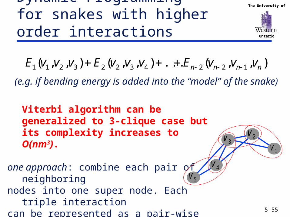
Dynamic Programming for snakes with higher order interactions

),,(...),,(),,( 12243223211 nnnn vvvEvvvEvvvE (e.g. if bending energy is added into the “model” of the snake)

Viterbi algorithm can be generalized to 3-clique case but its complexity increases to O(nm3).

one approach: combine each pair of neighboring nodes into one super node. Each triple interaction can be represented as a pair-wise interaction between 2 super-nodes. Viterbi algorithm will need m3 operations for each super node (why?)

1v2v

3v

4v

5v

The University of

Ontario

The University of

Ontario

5-56

DP snakes (open case)

Summary of Complexity

n

iii vE

1

)(

energy type complexity (order of interactions)

unary potentials O(nm) (d=1)

pair-wise potentials O((n-1)m2) (d=2)

triple potentials O((n-2)m3) (d=3)

complete connectivity O(mn) – exhaustive search (d=n)

2

121 ),,(

n

iiiii vvvE

1

11),(

n

iiii vvE

),...,,( 21 nvvvE

* - adding a single loop increases complexity by factor md-1

*

*

The University of

Ontario

The University of

Ontario

5-57

Problems with snakes

Depends on number and spacing of control points Snake may oversmooth the boundary Not trivial to prevent curve self intersecting

Can not follow topological changes of objects

The University of

Ontario

The University of

Ontario

5-58

Problems with snakes May be sensitive to initialization

– may get stuck in a local energy minimum near initial contour

Numerical stability can be an issue for gradient descent and variational methods (continuous formulation)• E.g. requires computing second order derivatives

The general concept of snakes (deformable models) does generalize to 3D (deformable mesh), but many robust optimization methods suitable for 2D snakes do not apply in 3D• E.g.: dynamic programming only works for 2D snakes

The University of

Ontario

The University of

Ontario

5-59

Problems with snakes

External energy: may need to diffuse image gradients, otherwise the snake does not really “see” object boundaries in the image unless it gets very close to it.

image gradientsare large only directly on the boundary

I

The University of

Ontario

The University of

Ontario

5-60

Diffusing Image Gradients Iimage gradients diffused via

Gradient Vector Flow (GVF)

Chenyang Xu and Jerry Prince, 98

http://iacl.ece.jhu.edu/projects/gvf/

The University of

Ontario

The University of

Ontario

5-61

Alternative Way to Improve External Energy

Use instead of where D() is

• Distance Transform (for detected binary image features, e.g. edges)

1n

0iiex )(DE v

1n

0iiex |)(I|E v

binary image features(edges)

Distance Transform ),( yxD

Distance Transform can be visualized as a gray-scale image

• Generalized Distance Transform (directly for image gradients)

The University of

Ontario

The University of

Ontario

5-62

Distance Transform (see p.20-21 of the text book)

34

23

23

5 4 4

223

112

2 1 1 2 11 0 0 1 2 1

0001

2321011 0 1 2 3 3 2

101110 1

2

1 0 1 2 3 4 3 210122

Distance Transform Image features (2D)

Distance Transform is a function that for each image pixel p assigns a non-negative number corresponding to

distance from p to the nearest feature in the image I

)(D)( pD

The University of

Ontario

The University of

Ontario

5-63

Distance Transform can be very efficiently computed

The University of

Ontario

The University of

Ontario

5-64

Distance Transform can be very efficiently computed

The University of

Ontario

The University of

Ontario

Distance Transform can be very efficiently computed

5-65

• Forward-Backward pass algorithm computes shortest paths in O(n) on a grid graph with regular 4-N connectivity and homogeneous edge weights 1

• Alternatively, Dijkstra’s algorithm can also compute a distance map (trivial generalization for multiple sources), but it would take O(n*log(n)).

- Dijkstra is slower but it is a more general method applicable to arbitrary weighted graphs

The University of

Ontario

The University of

Ontario

5-66

Distance Transform:an alternative way to think about

Assuming

then

is standard Distance Transform (of image features)

..

0)(

WO

featureimageisppixelifpF

)( pF

)( pD

Locations of binary image features

p

||||min)}(||{||min)(0)(:

qpqFqppDqFqq

The University of

Ontario

The University of

Ontario

5-67

Distance Transform vs.Generalized Distance Transform

For general

is called Generalized Distance Transform of

)}(||||{min)( qFqppDq

)( pF

F(p) may represent non-binary image features (e.g. image intensity gradient)

)( pF

)( pF

)( pDD(p) may prefer

“strength” of F(p)to proximity

q p

The University of

Ontario

The University of

Ontario

5-68

Generalized Distance Transforms(see Felzenszwalb and Huttenlocher, IJCV 2005)

The same “Forward-Backward” algorithm can be applied to any initial array • Binary ( ) initial values are non-essential.

If the initial array contains values of function F(x,y) then the output of the “Forward-Backward” algorithm is a Generalized Distance Transform

“Scope of attraction” of image gradients can be extended via external energy based on a generalized distance transform of

))(||||(min)( qFqppDIq

|)),((|),( yxIgyxF

/0

1

0

)(n

iiex vDE

The University of

Ontario

The University of

Ontario

5-69

Metric properties ofdiscrete Distance Transforms

- 1

1 0

0 1

1 -

Forward mask

Backward mask

Manhattan (L1) metric

Set of equidistantpoints

Metric

1.4 1

1 0

1.4 0

1.4 1

1

1.4Better approximationof Euclidean metric

In fact, “exact” Euclidean Distance transform can be computed fairly efficiently (in linear or near-linear time) without bigger masks1) www.cs.cornell.edu/~dph/matchalgs/2) Fast Marching Method –Tsitsiklis, Sethian

Euclidean (L2) metric

The University of

Ontario

The University of

Ontario

5-70

HW assignment 2 DP Snakes

• Use elastic snake model (value of l is important)

• Compare vs.

• Compare vs.

• Compare vs. where D is a

generalized distance transform of

such that (value of is important)

• Use Viterbi algorithm for optimization

• Incorporate edge alignment

• Use 3x3 search box for each control point

1

0

)(n

iiext vDE

1

0

)(n

iiext vFE

|)(| IgF

1

0

2int

n

iiLE

1

0

2int |ˆ|

n

ii LLE

extEEE lint

)}(||||{min)( qFqppDq

1n

0i

2iint LE

1n

0iiint |L|E