ct physics and instrumentation
TRANSCRIPT

CT Physics and
Instrumentation
Tim Marshel R.T.
(R)(N)(CT)(MR)(NCT)(PET)(CNMT)
SNMTS Approved
• 028617: CT Physics and Instrumentation
• CT Waiver Course
• Reference Number: 028617
• 1.5 SNMTS Voice Credits
• You must score greater than 80% in order to receive credit.

Program Objectives
• Describe the physics processes involved in the production of x-rays
• Describe the role of each component in the x-ray tube
• Discuss the role of proper adjustment of x-ray tube voltage and current in CT
• Name the principle parts of a CT scanner
• Discuss the function of each CT scanner component
• Discuss how CT image data are acquired and processed
• Describe the calculation process of Hounsfield units

Program Objectives • Describe CT number values assigned to various tissues
and how these values are assigned into meaningful display windowing
• Discuss CT image quality issues
• List the origin of CT image artifacts and describe their prevention
• Discuss appropriate parameters for the acquisition of low-dose CT for PET attenuation correction
• Describe the parameters and image characteristics required for a diagnostic-quality CT scan
• Discuss the importance of CT quality control
• Review GE‟s Discovery Light-Speed CT Scanner configuration

Introduction
• This will provide an overview of the principles and operation of a computed tomography (CT) scanner as well as look at Image data acquisition, CT image construction , display, image quality protocols, artifacts, radiation safety and quality control
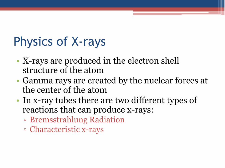
Physics of X-rays
• X-rays are produced in the electron shell structure of the atom
• Gamma rays are created by the nuclear forces at the center of the atom
• In x-ray tubes there are two different types of reactions that can produce x-rays:▫ Bremsstrahlung Radiation▫ Characteristic x-rays
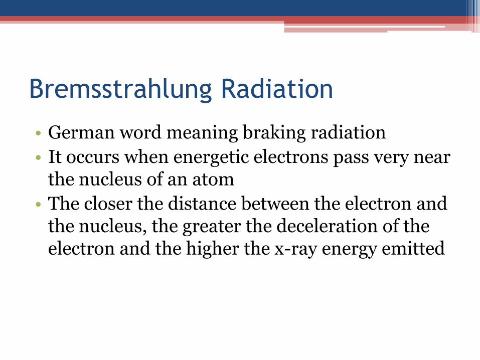
Bremsstrahlung Radiation
• German word meaning braking radiation
• It occurs when energetic electrons pass very near the nucleus of an atom
• The closer the distance between the electron and the nucleus, the greater the deceleration of the electron and the higher the x-ray energy emitted
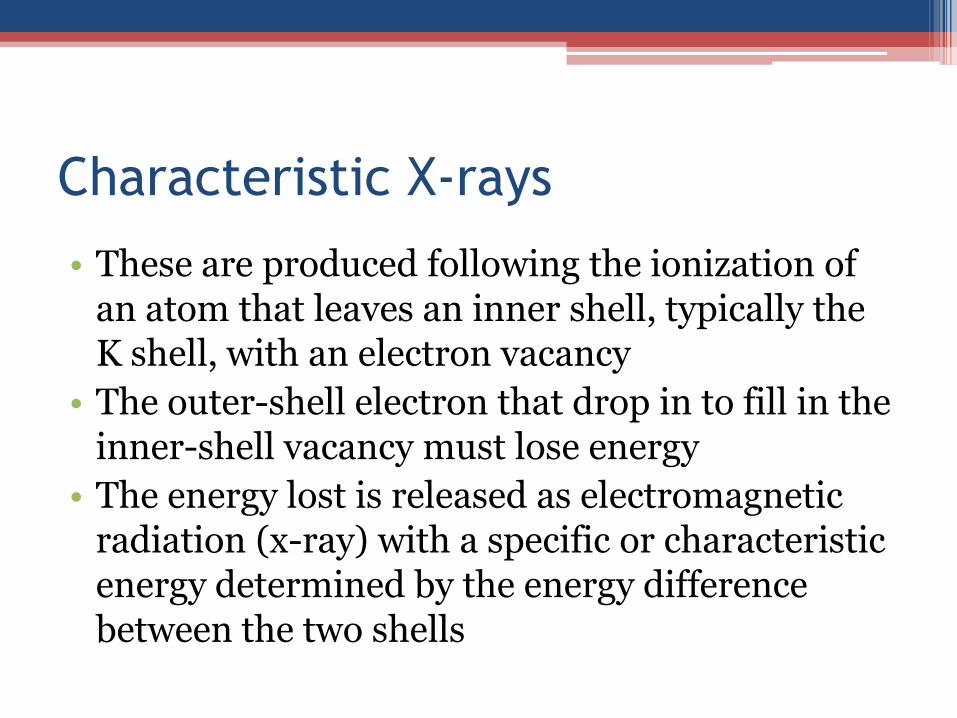
Characteristic X-rays
• These are produced following the ionization of an atom that leaves an inner shell, typically the K shell, with an electron vacancy
• The outer-shell electron that drop in to fill in the inner-shell vacancy must lose energy
• The energy lost is released as electromagnetic radiation (x-ray) with a specific or characteristic energy determined by the energy difference between the two shells

X-ray Tube design
• The x-ray tube is a glass envelope that contains a high vacuum so that accelerated electrons from the internal electrodes may move with ease
• Within the x-ray tube is a cathode that has a very small filament, which is several millimeters in length
• X-ray tubes for CT scanners have an anode that rotates thousands of revolutions per minute in order to prevent the beam of electrons from the cathode from burning the anode and to remove heat from the anode
• X-ray tubes in CT scanners may use standard, high-resolution, and sometimes ultrahigh-resolution focal spot sizes and secondary collimation to improve image resolution
Voltage Variation
• An increase in the high voltage applied to the x-ray tube will result in a corresponding increase in the maximum energy of the x-rays that are produced
Energies required
• For typical PET/CT studies of the body that range will be 80-140kVp(peak kilovoltage)
• This also depends on the size of the patient and the detail that is required
• The energies that can be selected on a CT scanner are usually defined by a limited set of energies such as 80, 100, 120, and 140kVp
• A general rule is that an increase of approximately 15% in kVp is roughly equivalent to doubling the milliampereseconds (mAs)
Tweaking kVp for Scanning
• Higher-energy x-ray photons are needed to penetrate large bones of the shoulder, hip and vertebrae
• The kVp setting also defines the fraction of photons that will successfully reach the detectors of the scanner
• Higher-energy photons are less attenuated by the body
• More photons reaching the detectors will result in lower quantum noise in the images, but the radiation exposure to the patient will increase
Beam Hardening
• The spectrum of x-rays passes though the body, the lower-energy (softer) x-rays are most easily absorbed
• As the beam passes though there is a shift in energy distribution so that a larger fraction of the remaining photons have a higher energy; this spectral shift is called beam hardening
• Beam hardening will create artifacts seen as dark streaks that radiate from the outside toward the inner part of the body

Advantages and disadvantages of
using a higher kVpAdvantages
• Greater penetration through the body
• Decrease in quantum noise
• A reduction in beam hardening artifacts
Disadvantages
• Higher dose to patient
• Reduces differences in tissue densities

Current Variation
• The applied current is another factor that can be adjusted in the x-ray tube
• There is a proportional increase in the number of x-rays, at all energies, when the current in milliampere (mA) is increased
• Both the Bremsstrahlung and characteristic x-rays that are produced increase proportionally with the current

Current Variation in CT
• The range of currents that may be used in CT Scanner is commonly very wide, about 50-400mA
• It is continually variable and typically does not limit the operator to a few preset values
• The mA is a direct defining parameter of the number of photons generated by the x-ray tube
• The mA and the time are the dominant parameters that determine the radiation dose to the patient

Advantages and Disadvantages of
Current VariationAdvantages
• Decrease in image noise
• Increase in contrast resolution
Disadvantages
• Higher mA increases dose to the patient
X-ray Filter
• Both planar x-ray and CT imaging system position an absorbing x-ray filter into the x-ray beam
• The beam-modifying filter has tow purposes:▫ Filtering absorbs low energy x-rays that would
attenuate in the body and create noise; this would improve the image. The filter also reduces patient radiation exposure by as much as 50%
▫ Filtering also helps in shaping the energy distribution of the beam. A filter also aids in preventing the edges of the beam from hardening and this makes the distribution more uniform

Filters on a CT scanner
• The filters on a CT scanner is not interchangeable with other filters
• It is a permanent installation for modifying the beam as mentioned and reduces the unused low-energy radiation, which adds nothing to the image formation
Principles of Computed
Tomography
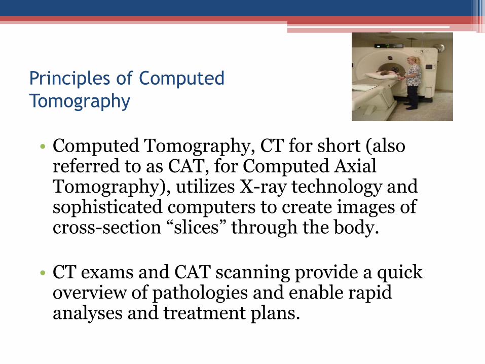
• Computed Tomography, CT for short (also referred to as CAT, for Computed Axial Tomography), utilizes X-ray technology and sophisticated computers to create images of cross-section “slices” through the body.
• CT exams and CAT scanning provide a quick overview of pathologies and enable rapid analyses and treatment plans.
Principles of Computed
Tomography• Tomography is a term that refers to the
ability to view an anatomic section or slice through the body.
• Anatomic cross sections are most commonly refers to transverse axial tomography.
• CT scanner was developed by Godfrey Hounsfield in the very late 1960s.

Contd…
• This x-ray based system created projection information of x-ray beams passed through the object from many points across the object and from many angles (projections).
• Early CT scanners were limited to use in the brain.• In 1974 Robert Ledley introduced techniques that led to
the development of the first CT scanner that could perform whole-body imaging of patients.
• CT produces cross-sectional images and also has the ability to differentiate tissue densities, which create an improvement in contrast resolution.
CT Scanner Design
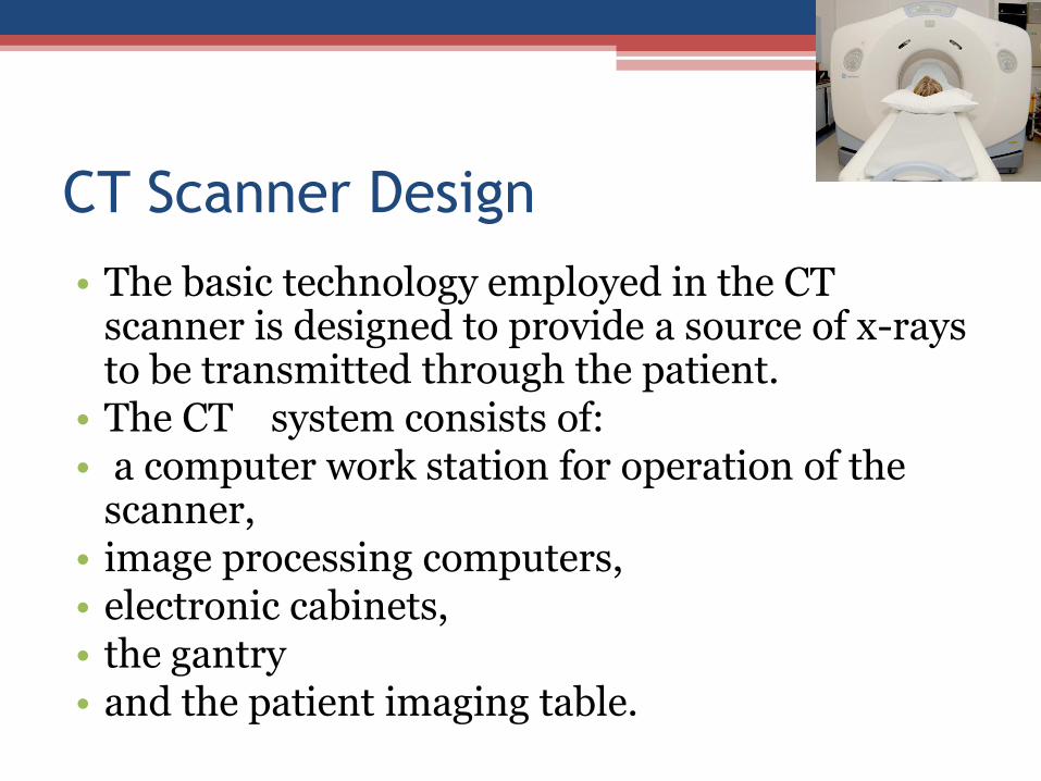
• The basic technology employed in the CT scanner is designed to provide a source of x-rays to be transmitted through the patient.
• The CT system consists of:• a computer work station for operation of the
scanner, • image processing computers,• electronic cabinets, • the gantry• and the patient imaging table.

Composition of the Gantry
• The gantry houses the key components of the scanner.• Many components associated with the production of the
x-ray beam and detection and acquisition of the beam must be located within the rotating portion of the gantry.
• The fan-beam x-ray tube sits opposite the detector array within the rotating gantry.
• The three phase power generator is also within the gantry module.
• Heat from the generator, x-ray tube, and other components must be removed efficiently.

Contd…
• The x-ray tube in a CT scanner is designed to produce a fan beam of x-rays that is approximately as wide as the body.
• Tissue attenuation is measured over a large region from one position of the x-ray tube.
• The x-ray tube on a CT scanner is a much more heavy duty unit than the tubes used for standard x-ray imaging.
• On the opposite side of the patient is the detector array that measures the strength of the x-ray beam at various points laterally across the body.
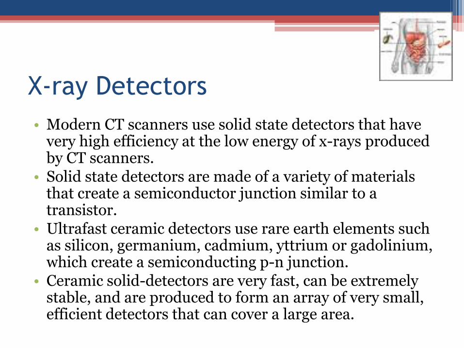
X-ray Detectors
• Modern CT scanners use solid state detectors that have very high efficiency at the low energy of x-rays produced by CT scanners.
• Solid state detectors are made of a variety of materials that create a semiconductor junction similar to a transistor.
• Ultrafast ceramic detectors use rare earth elements such as silicon, germanium, cadmium, yttrium or gadolinium, which create a semiconducting p-n junction.
• Ceramic solid-detectors are very fast, can be extremely stable, and are produced to form an array of very small, efficient detectors that can cover a large area.
contd…
• Detector systems in a multiple-slice CT scanners use detectors that are in a multiple transverse line across the patient in a two-dimensional (2D) array.
• The array size for a 16 slice CT may have more than 800 detector elements laterally across the gantry.
• The size of the individual detector elements is less than 1 mm on each side.
Collimation
• CT scanners use collimators to protect the patient and limit the beam to the size of the detector array that is active during data acquisition.
• The configuration of CT collimation is adjacent to the x-ray tube.
• It restricts the width and shape the beam to the area of interest for a single rotation of the tube and detectors around the patient.
Contd…
• The slice thickness that may be reconstructed can never be thinner than the collimator width.
• Selecting an appropriate collimation thickness will prevent small lesions from being missed.
• Thinner collimation produces less streaking of high density objects.
• Collimation should be sufficiently thinner than the lesions to be detected.
• Slice thickness is important because it defines the volumetric dimension of the image voxels.

Advantages and disadvantages of thinner
collimation
• Advantages are:
• Less volume averaging
• Better resolution on reformatted sagittal and coronal images
• Increased spatial resolution
• Fewer streaking artifacts from high-density objects.
Contd…
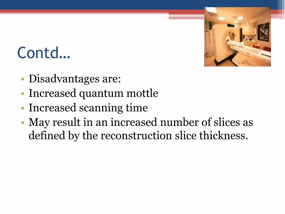
• Disadvantages are:
• Increased quantum mottle
• Increased scanning time
• May result in an increased number of slices as defined by the reconstruction slice thickness.

Rotation Speed
• The rotation speed is the time required for the gantry to make one complete revolution.
• In helical (spiral) CT the gantry rotates continuously in one direction on the slip-ring system,
• While the patient table moves at a constant speed through the gantry to quickly perform the scan of a relatively large body area.
• Faster CT rotation speeds may be desirable for reducing the likelihood of patient motion artifacts.
Pitch
• In helical CT, pitch is the ratio of the patient‟s movement through the gantry during one 360 degree rotation relative to the beam collimation.
• For single slice CT, Pitch is equal to the table movement per rotation divided by slice collimation.
• On most CT and PET/CT systems the pitch is entered as a parameter that is set in defining the procedure for the acquisition of patient data.
• When the pitch is greater than 1.0 mm, there are interspaces created and some portion of the body is being missed.
Increment
• The increment is the distance between the slices.• In CT data are acquired as projection
information along the helical path.• Slices may be reconstructed at various positions
along the helix.• One important factor in defining the slices and
their positional relationship to one another is the distance between the reconstructed axial slices in the „z‟ direction.

Image Data Acquisition
• The high performance of CT scanners creates a volume of reconstructed data instead of a group of slices
• The data acquired from the helical motion of the gantry are obtained as projection information, as in both SPECT and PET
• The raw data may be used to create several image sets to reveal different information from just the one set of raw data

Image Data Acquisition cont’d
• An example is the raw data may be used to generate one set of data to be used for attenuation correction of SPECT or PET
• Another reconstruction set of images may be high-resolution thin slices, but another may be smoother, thicker slices
• The beam width as set by the detector size and collimator determines the maximum resolution that may be obtained in the study
• A typical CT acquisition for combined SPECT/CT or PET/CT may take less than 1 minute
CT Image Reconstruction
• The reconstruction of a multislice CT images will be computed from the helical projection data
• Since the x-ray beam is either fan-shaped or cone-shaped in a helical pattern, special reconstruction algorithms are used to account for this unique geometry
• Image reconstruction may use different reconstruction algorithms that will calculate the attenuation at each pixel in the slice
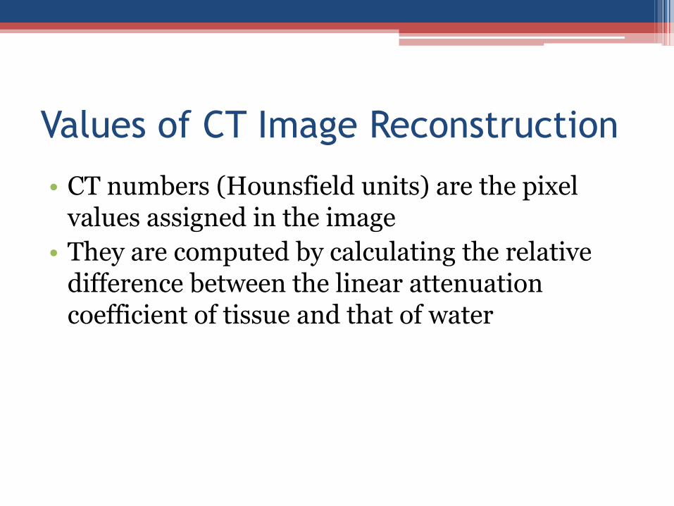
Values of CT Image Reconstruction
• CT numbers (Hounsfield units) are the pixel values assigned in the image
• They are computed by calculating the relative difference between the linear attenuation coefficient of tissue and that of water
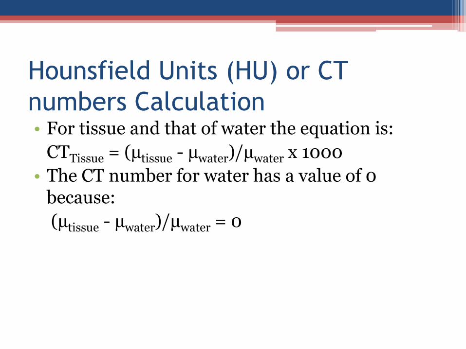
Hounsfield Units (HU) or CT
numbers Calculation• For tissue and that of water the equation is:
CTTissue = (µtissue - µwater)/µwater x 1000
• The CT number for water has a value of 0 because:
(µtissue - µwater)/µwater = 0
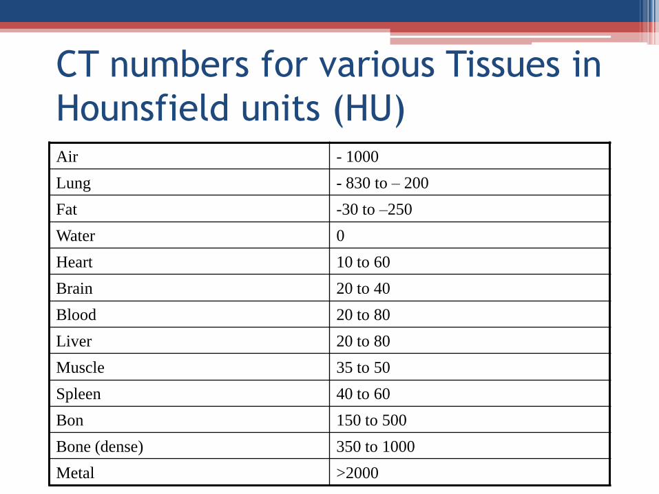
CT numbers for various Tissues in
Hounsfield units (HU)Air - 1000
Lung - 830 to – 200
Fat -30 to –250
Water 0
Heart 10 to 60
Brain 20 to 40
Blood 20 to 80
Liver 20 to 80
Muscle 35 to 50
Spleen 40 to 60
Bon 150 to 500
Bone (dense) 350 to 1000
Metal >2000

Algorithms used in CT Image
Reconstruction• A variety of algorithms have been used to
reconstruct CT images:
▫ Filtered back-projection (FBP)
▫ Iterative algorithms
Reconstruction Kernels
• This is another important parameter that is set prior to CT reconstruction
• The kernel is an algorithm that, in the case of CT reconstruction, defines the clinical application and amount of smoothing that will be applied in the reconstruction process
• Each vendor‟s CT scanner will have a variety of kernels that optimize the image quality to a particular body area or tissue type
• Bone images will require an algorithm that maintains sharpened edges or bone margins

Example of Kernels in
Reconstruction• An example is a Siemens system the kernels are
defined by a letter (or letters) followed by a number• The letter identifies the body area or clinical
application (e.g H=head, B=body, U=ultrahigh resolution, C=Child head)
• The typical numbers ranges from 10-90• Most clinically useful filters use numbers in the
range of 30 to 40• The higher the kernel number, the shaper the image• On the other hand the lower the number the
smoother the image
Advantages and Disadvantages of
CT image reconstructionAdvantages
• Desired image detail is obtained• Filters may sharpen or smooth reconstructed
images• Raw data may be reconstructed post-acquisition
with a variety of filtersDisadvantages
• Multiple reconstructions may be required if significant detail is required from areas of the study that contain bone and soft tissue

Post-processing Filtering
• A post-processing filter such as low-contrast enhancement (LCE) filter will improve low-contrast resolution while it decreases image noise
• A high-contrast enhancement (HCE) filter will produce sharpening of high-contrast differences as in the head imaging and brain imaging

CT Display
• Digital image display of CT information creates unique challenges due to the wide variation in CT numbers in the image
• An example is the chest region contains lung tissue (CT numbers in the range of –850 to –200), fat (-250 to –30), soft tissue (10 to 80), and bone (150 to 500 or more)
• This range of CT numbers in the image is from –850 to 500 numbers

Limitations of CT display
• The human eye is thought to be able to discern only 30 to 100 different shades of gray; because of this only a limited range of CT values are displayed in the image
• Digital imaging is often limited to 8 bits of data and therefore only 256 intensity values are assigned over the entire gray scale from black to white

Examples of CT window selection
• A bone window may be set with CT values selected from 400 to 1000 to view details of the dense bone in the vertebrae
• Windowing from CT numbers 0 to –1200 allows the lung tissue to be viewed
• While windowing from –85 to 165 creates a scale to better evaluate soft tissue

Display of Volumetric Image Data
• Some of the most dramatic display options are those that allow the CT data to be depicted as though the true anatomy of the patient were being visualized
• Although these images are attention-grabbing they typically have little use to the radiologist in interpreting the examination
• But it can have useful application in surgical planning and marketing radiology studies
• Computed tomography images are also the standard display used in radiation therapy treatment planning
MIP
• Maximum intensity projection (MIP) images are generated by taking a stack of image slices and projecting back the maximum intensity of the brightest pixel along that path
• This technique uses the same principles as MIP imaging for SPECT and PET
SSDs
• The creation of shaded surface displays (SSDs) images is typically done in three steps:▫ Reconstruct the CT data from the 2D slices using thin
overlapping slices
▫ Segment out unwanted data using thresholding of the CT numbers or cropping or segmenting out overlying structures
▫ Render or shade the projected images to provide depth perception and illumination of the patient
Image Quality
• Although CT images are relatively simple displays, the generation of the images is based on settings and parameters, as well as some some others
• Each parameter setting that is selected prior to imaging will have some effect on the final image

Contrast Resolution
•Ability to differentiate between different tissue densities in the image
–High-Contrast
–Low-Contrast

High-Contrast Resolution• Ability to see small objects and details that have high density difference compared with background.
▫ very high density difference from one another
Ability to see a small, dense lesion in lung tissue
See objects where bone and soft tissue are adjacent.
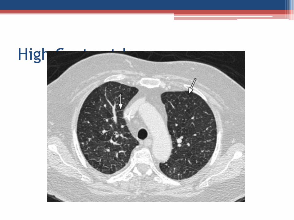
High Contrast Image

Low-Contrast Resolution• Ability to visualize objects that have very little difference in density from one another.
▫ Better when there is very low noise
Visualizing soft-tissue lesion within the liver.
Differentiate gray matter from white matter in the brain.

Low Contrast image

Image Noise
• Noise level: % of contrast
▫ Number of detected photons
▫ Matrix size
▫ Slice thickness
▫ Algorithm
▫ Electronic noise
▫ Scattered radiation
▫ Object size.

CT Protocols• All CT scans begin by performing a scout scan.
▫ used in planning the exam and to establish where the target organs are located.
Not critical for examination
Operator should limit radiation exposure to paient from scout scan.
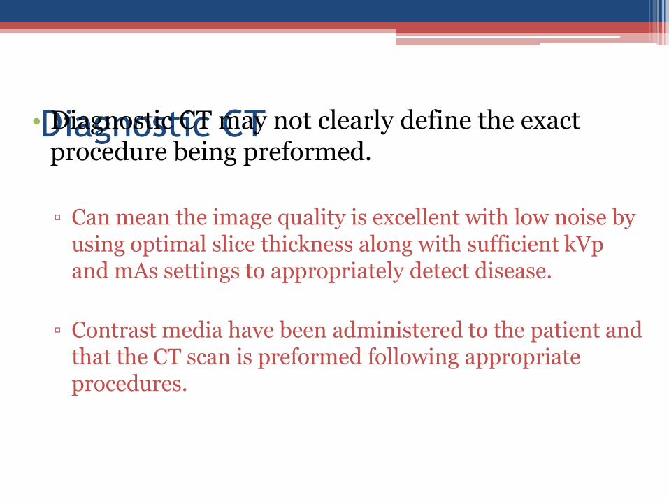
Diagnostic CT• Diagnostic CT may not clearly define the exact procedure being preformed.
▫ Can mean the image quality is excellent with low noise by using optimal slice thickness along with sufficient kVp and mAs settings to appropriately detect disease.
▫ Contrast media have been administered to the patient and that the CT scan is preformed following appropriate procedures.

CT Artifacts
• Artifacts can degrade image quality and affect the perceptibility of detail.
• Includes
▫ Streaks
▫ Rings and bands
▫ Shading
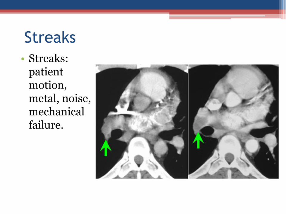
Streaks
• Streaks: patient motion, metal, noise, mechanical failure.
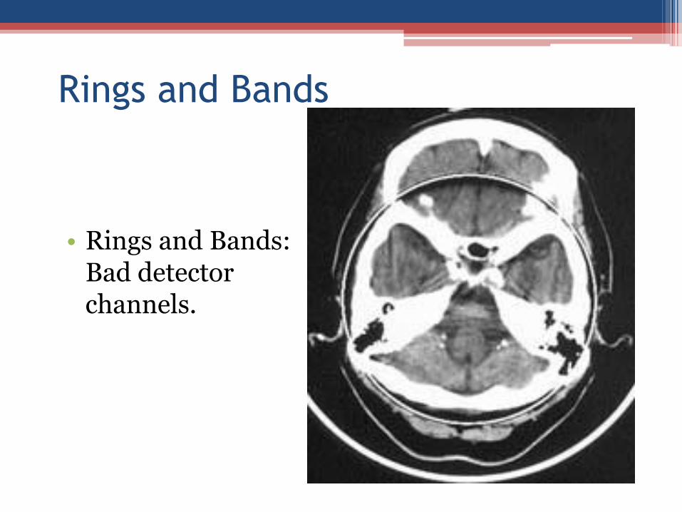
Rings and Bands
• Rings and Bands: Bad detector channels.

Shading
Shading can occur due to incomplete projections.

Quality Control
• The definition of QC consists of 2 parts.▫ Quality assurance requires a measurement of the
CT scanner‟s performance to ensure the scanner is operating at some acceptable level.
▫ Quality control carries the concept of quality assurance one step further – if the quality is inadequate, then steps are taken to correct the problem.

Why do we need QC?
• Maintain high performance standards for our patiant's
• Regulatory agencies demand QC on equipment that can potentially harm patients
▫ Examples:
Mechanical parts wear slowly.
Electronic parts can change characteristics and drift out of optimal adjustment.

LightSpeed16

Hardware Components
• Collimator
▫ Two independently controlled tungsten cams. The rotation of cams provides continuous variable slice thickness and z-axis position

Scan GeometryGantry aperture: HiSpeed 70 cm, LightSpeed 70cm
Focus to isocenter: HiSpeed 63 cm, LightSpeed 54 cm
Focus to detector: HiSpeed 110 cm, LightSpeed 95 cm
Maximum SFOV: HiSpeed 48 cm, LightSpeed 50 cm
Allows 20% mAs reduction
CTi Focal Spot
Detector
LightSpeed Focal
Spot
Detector

Hardware Components
• Changes in the DAS, Slip Ring, and detector have been made.
• New reconstruction algorithms for 16 slice multi-slice data.

Key Points to review…..
• Describe the axial and helical 8 slice configurations
• Explain how signal/data are collected in each configuration
• Explain how slice thickness options are affected by detector configuration in axial and helical modes
• Identify the pitch and table speed options available for each 8 slice and 16 configuration
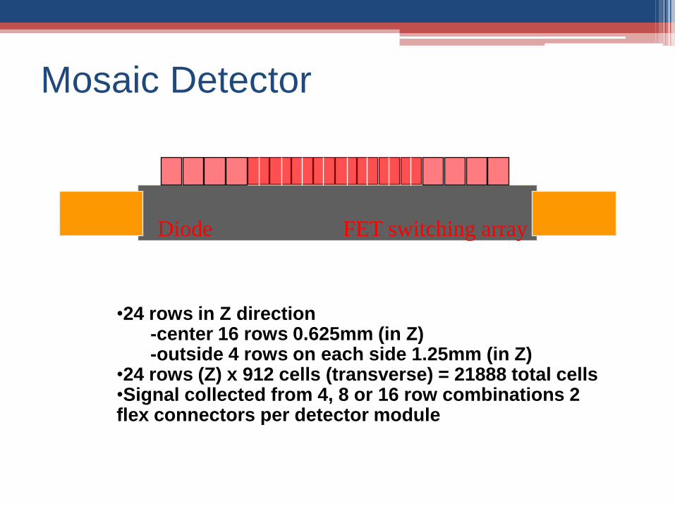
Mosaic Detector
•24 rows in Z direction-center 16 rows 0.625mm (in Z)-outside 4 rows on each side 1.25mm (in Z)
•24 rows (Z) x 912 cells (transverse) = 21888 total cells•Signal collected from 4, 8 or 16 row combinations 2 flex connectors per detector module
Diode FET switching array

Mosaic Detector

Detector Configurations
16 x 0.625 mmX-ray Tube Focal Spot
X-ray Beam Collimator16 signals collected per
gantry rotation from 16
detectors with 1 detectors
contributing to each
signal
0.625 mm slices are the
minimum
10 mm of coverage per
rotation
Diode FET Switching Array
Diode FET Switching Array

Detector Configurations
16 x 1.25 mmX-ray Tube Focal Spot
X-ray Beam Collimator16 signals collected per
gantry rotation from 24
detectors with 1 and 2
detectors contributing to
each signal
1.25 mm slices are the
minimum because two 0.625
mm detectors are combined
per signal
(2 x 0.625 = 1.25) for center 8
signals
And 1x1.25 for each outside 4
20 mm coverage per rotation
Diode FET Switching Array
Diode FET Switching Array

Detector Configurations
8 x 1.25 mmX-ray Tube Focal Spot
X-ray Beam Collimator8 signals collected per
gantry rotation from 16
detectors with 2
detectors contributing to
each signal
1.25 mm slices are the
minimum because two
0.625 mm detectors are
combined per signal
(2 x 0.625 = 1.25)
10 mm of coverage per
rotation
Diode FET Switching Array
Diode FET Switching Array
Detector Configurations
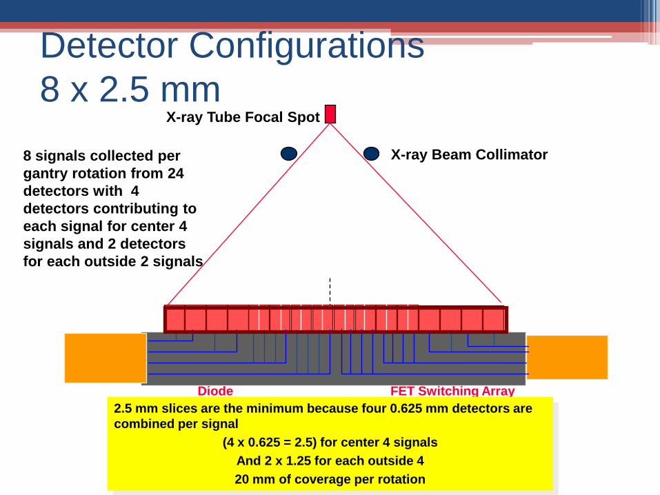
8 x 2.5 mmX-ray Tube Focal Spot
X-ray Beam Collimator
Diode FET Switching Array
2.5 mm slices are the minimum because four 0.625 mm detectors are
combined per signal
(4 x 0.625 = 2.5) for center 4 signals
And 2 x 1.25 for each outside 4
20 mm of coverage per rotation
8 signals collected per
gantry rotation from 24
detectors with 4
detectors contributing to
each signal for center 4
signals and 2 detectors
for each outside 2 signals
Detector Configurations
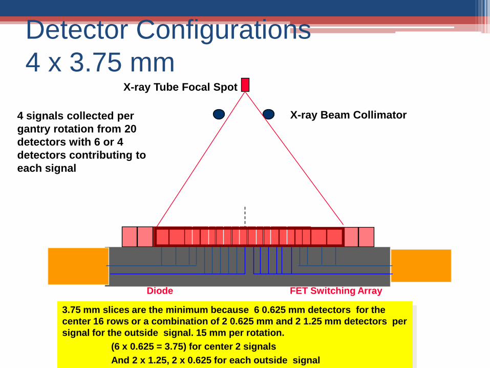
4 x 3.75 mmX-ray Tube Focal Spot
X-ray Beam Collimator
Diode FET Switching Array
3.75 mm slices are the minimum because 6 0.625 mm detectors for the
center 16 rows or a combination of 2 0.625 mm and 2 1.25 mm detectors per
signal for the outside signal. 15 mm per rotation.
(6 x 0.625 = 3.75) for center 2 signals
And 2 x 1.25, 2 x 0.625 for each outside signal
4 signals collected per
gantry rotation from 20
detectors with 6 or 4
detectors contributing to
each signal

Detector Configurations
4 x 1.25 mmX-ray Tube Focal Spot
X-ray Beam Collimator
Diode FET Switching Array
5mm coverage per rotation
4 signals collected per
gantry rotation from 8
detectors with 2 detectors
contributing to each
signal

Detector Configurations2 x 0.625mm
X-ray Tube Focal Spot
X-ray Beam Collimator
Diode FET Switching Array
2 signals collected from two
0.625 mm detector row with
one detector row
contributing to the signal. 0.625 mm slices are the minimum
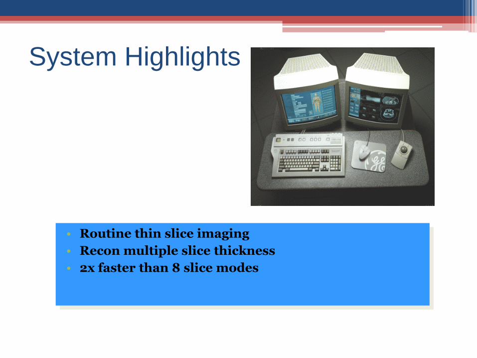
System Highlights
• Routine thin slice imaging
• Recon multiple slice thickness
• 2x faster than 8 slice modes

16 Slice System Highlights• Detector Design
▫ Comprised of 2 row sizes
▫ 24 rows total
▫ 20mm coverage
• Xray beam collimation
-Tracking determines scan modes
- 8 or 16 X acquisition modes
• Xray detection
▫ New scaleable multislice detector and DAS
▫ 96 convertor boards
▫ 1640 hz maximum sample rate
Increases # of views at 0.5 sec. to 820
full views at 0.6 second
• Image processing and reconstruction
▫ New Z-smoothing factors
▫ Full and Plus recon for optimized slice profiles
▫ Recon processing to minimize MIP artifacts

Axial Signal Collection • 16 signals/ 24 rows can be collected per gantry rotation
• Each of the 16 signals can be collected from an individual detector or a combination of 2, 4 or 8 detectors
• Once signal from multiple detectors has been combined into a channel, it cannot be separated
• The number of detectors combined per signal/channel affects the minimum slice thickness
• 16 slices can be generated per slice rotation
• Slice thickness can be increased retrospectively
• Detector configuration at time of acquisition affects the retrospective choices

Axial Configurations16 x 0.625 mm
16 signals collected from sixteen 0.625 mm detectors with 1 detectors contributing to each signal
0.625 mm is the minimum slice thickness. 10 mm coverage per rotation
Cells can be combined to form 16 slices @ 0.625 mm, 8 slices @ 1.25 mm, 4 slices @ 2.5 mm, 2 slices @
5mm and 1 slice @ 10 mm
16i mode = 1 row
Each cell becomes a slice
@ 0.625 mm each
5
8i mode = 2 cells
combined become a slice
@ 1.25 mm each
4i mode = 4 cells
combined become a slice
@ 2.5 mm each
2i mode = 8 cells
combined become a slice
@ 5 mm each
3 9 10 13 151 2 4 6 7 8 11 12 14 16 1 2 3 4 5 6 7 8 21 3 4
1 2 1
1i mode = 16 cells
combined become a slice
@ 10 mm
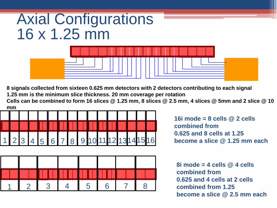
Axial Configurations16 x 1.25 mm
8 signals collected from sixteen 0.625 mm detectors with 2 detectors contributing to each signal
1.25 mm is the minimum slice thickness. 20 mm coverage per rotation
Cells can be combined to form 16 slices @ 1.25 mm, 8 slices @ 2.5 mm, 4 slices @ 5mm and 2 slice @ 10
mm
16i mode = 8 cells @ 2 cells
combined from
0.625 and 8 cells at 1.25
become a slice @ 1.25 mm each1 2 161514131211109876543
1 2 3 4 5 6 7 8
8i mode = 4 cells @ 4 cells
combined from
0.625 and 4 cells at 2 cells
combined from 1.25
become a slice @ 2.5 mm each
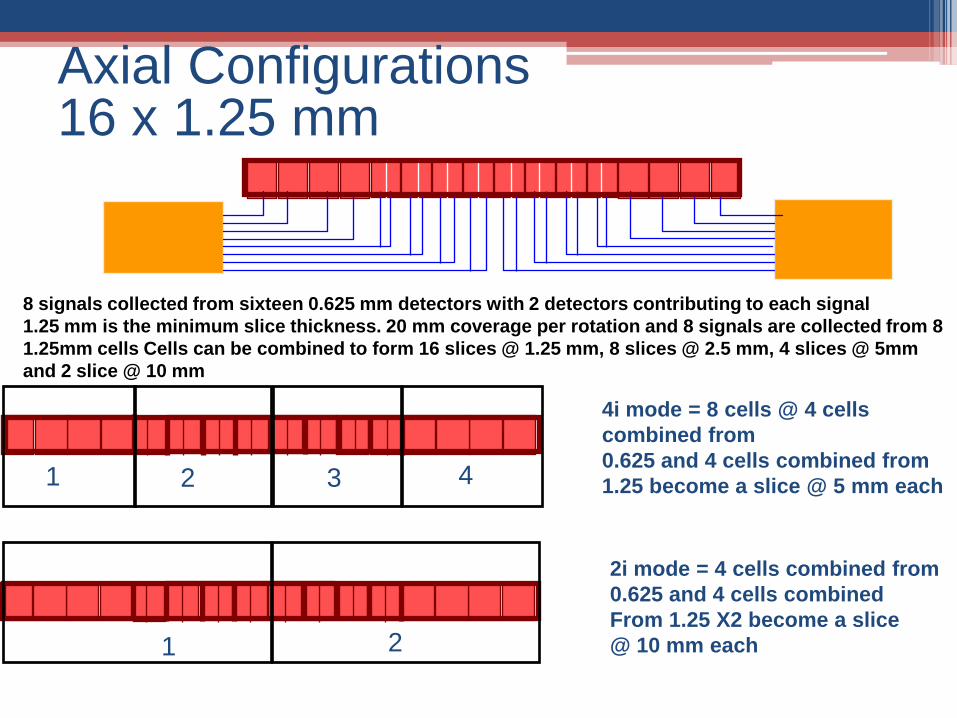
Axial Configurations16 x 1.25 mm
8 signals collected from sixteen 0.625 mm detectors with 2 detectors contributing to each signal
1.25 mm is the minimum slice thickness. 20 mm coverage per rotation and 8 signals are collected from 8
1.25mm cells Cells can be combined to form 16 slices @ 1.25 mm, 8 slices @ 2.5 mm, 4 slices @ 5mm
and 2 slice @ 10 mm
4i mode = 8 cells @ 4 cells
combined from
0.625 and 4 cells combined from
1.25 become a slice @ 5 mm each
2i mode = 4 cells combined from
0.625 and 4 cells combined
From 1.25 X2 become a slice
@ 10 mm each
1 2 3 4
1 2

Axial Configurations8 x 1.25 mm
8 signals collected from sixteen 0.625 mm detectors with 2 detectors contributing to each signal
1.25 mm is the minimum slice thickness. 10 mm coverage per rotation
Cells can be combined to form 8 slices @ 1.25 mm, 4 slices @ 2.5 mm, 2 slices @ 5mm and 1 slice @ 10
mm
8i mode = 1 signal
become a slice
@ 1.25 mm each
1 2 3 54 6 7 8
4i mode = 4 signals
become a slice
@ 2.5 mm each
1 2
2i mode = 8 signals
become a slice
@ 5 mm each
1
1i mode = 8 signals
become a slice
@ 10 mm each
1 2 3 4
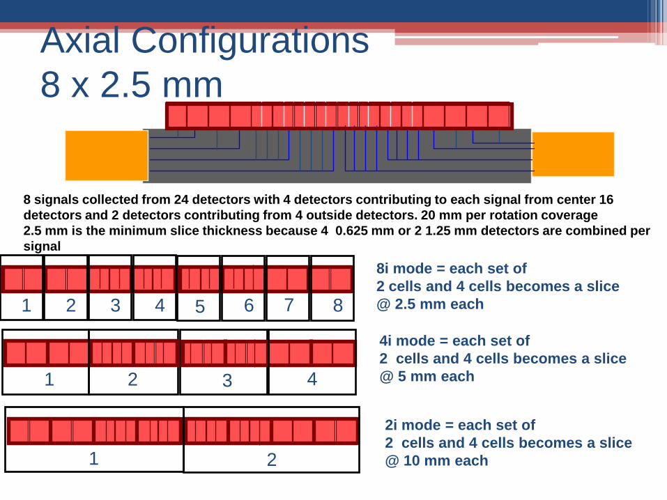
Axial Configurations
8 x 2.5 mm
8 signals collected from 24 detectors with 4 detectors contributing to each signal from center 16
detectors and 2 detectors contributing from 4 outside detectors. 20 mm per rotation coverage
2.5 mm is the minimum slice thickness because 4 0.625 mm or 2 1.25 mm detectors are combined per
signal
8i mode = each set of
2 cells and 4 cells becomes a slice
@ 2.5 mm each1 2 3 4 6 85 7
1 2 3 4
4i mode = each set of
2 cells and 4 cells becomes a slice
@ 5 mm each
1 2
2i mode = each set of
2 cells and 4 cells becomes a slice
@ 10 mm each

Axial Configurations4 x 3.75 mm
4 signals collected from twelve 1.25 mm detectors with 3 detectors contributing to each signal
3.75 mm is the minimum slice thickness because three 1.25 mm detectors are combined per signal
Sets of cells can be combined to create 4 slices @ 3.75 mm each or 2 slices @7.5 mm each 15 mm
coverage per rotation
Diode FET Switching Array
2i mode = 2 sets (of 3 cells each)
are combined to form 2 slices
@ 7.5 mm each
4i mode = each set of
3 cells becomes a slice
@ 3.75 mm each
1 2 3 4 1 2

Detector Configurations
4 x 1.25 mm
Diode FET Switching Array
5mm coverage per rotation
Used for Biopsy 5mm/1i
4 signals collected per gantry rotation from 8
detectors with 2 detectors contributing to each
signal
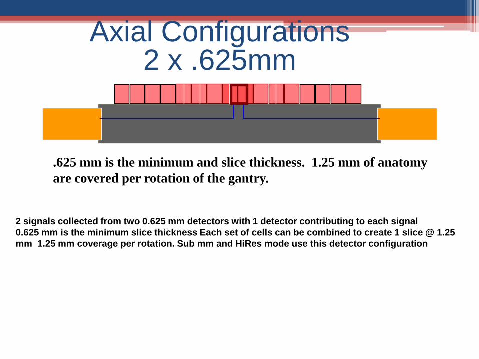
Axial Configurations2 x .625mm
.625 mm is the minimum and slice thickness. 1.25 mm of anatomy
are covered per rotation of the gantry.
2 signals collected from two 0.625 mm detectors with 1 detector contributing to each signal
0.625 mm is the minimum slice thickness Each set of cells can be combined to create 1 slice @ 1.25
mm 1.25 mm coverage per rotation. Sub mm and HiRes mode use this detector configuration

Axial Interface•Select Number of Rows
•Select slice thickness and
number of images per rotation
•System displays retrospective
choices based on prospective
detector configuration
16 Row
• 0.625/16i 1.25/16i
• 1.25/8i 2.5/8i
• 2.5/4i 5/4i
• 5/2i 10/2i
• 10/1i
8 Row
• 1.25/8i 2.5/8i
• 2.5/4i 5/4i
• 5/2i 10/2i
• 10/1i
4 Row 2 Row
• 3.75/4i 0.625/2i (sub mm)
• 7.5/2i 1.25/1i (HiRes)
•To calculate detector
configuration in axial mode
Row selection and
minimum thickness
determines

Axial Interface
axial demo.ppt
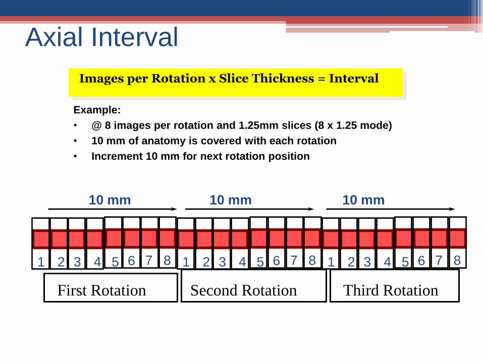
Axial Interval
Images per Rotation x Slice Thickness = Interval
Example:
• @ 8 images per rotation and 1.25mm slices (8 x 1.25 mode)
• 10 mm of anatomy is covered with each rotation
• Increment 10 mm for next rotation position
10 mm 10 mm10 mm
1 2 3 54 6 7 8 1 2 3 54 6 7 8 1 2 3 54 6 7 8
First Rotation Second Rotation Third Rotation

Axial Interval with SkipImages per Rotation x Slice Thickness + Gap = Interval with
Skip
Example:
• @ 8 images per rotation and 1.25 mm slices if a 10 mm gap is desired between
the last slice of the preceding group and the first slice of the succeeding group
• Increment 10 mm (total anatomy covered per rotation) plus 10 mm (the desired
gap) for a total of 20 mm for the next rotation position
10 mm scanned
10 mm gap
10 mm scanned
20 mm interval
1 2 3 54 6 7 8
First Rotation
1 2 3 54 6 7 8
Second Rotation

Tilt Correction
Z axis increment =
slice thickness
No Gantry Tilt
Slice thickness
measured
perpendicular
to slice edges
Gantry Tilt
Z axis increment is greater
than slice thickness due to tilt
Slice thickness remains
the same measured
perpendicular
to slice edgesZ axis increment
equals distance
between slice centers
Distance between slice
centers elongates with
a tilt when projected to
the Z axis
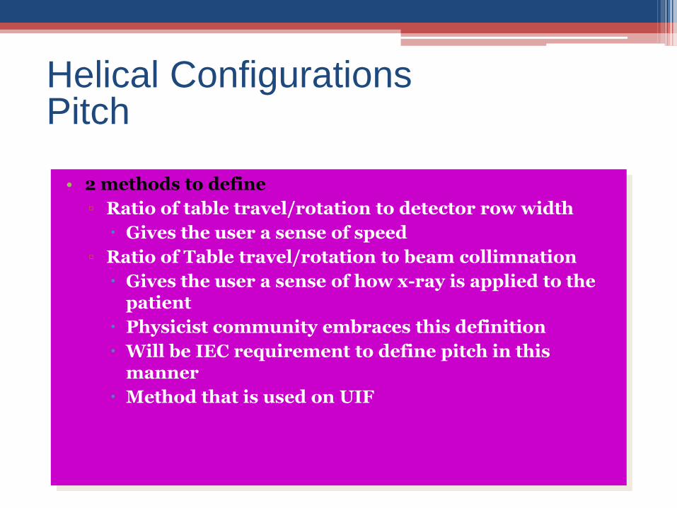
Helical Configurations Pitch
• 2 methods to define
▫ Ratio of table travel/rotation to detector row width
Gives the user a sense of speed
▫ Ratio of Table travel/rotation to beam collimnation
Gives the user a sense of how x-ray is applied to the patient
Physicist community embraces this definition
Will be IEC requirement to define pitch in this manner
Method that is used on UIF

Helical Configurations
• In one helical scan 8 or 16 interleaved or 8 or 16 interspaced helices are collected from 16 or 24 detectors to form a volumetric data set
• A new helical reconstruction algorithm uses data from all 8 or 16 helices to generate each image
▫ Helical weighting algorithms tailored to each pitch mode allow mAs reduction and reduce helical artifact
▫ Slice thickness affected by detector configuration and helical reconstruction algorithm
• Slice thickness can be changed retrospectively
• 4 preferred pitches 8X: 0.625:1, 0.875:1, 1.35:1 and 1.675:1
• 4 preferred pitches 16X: 0.5625:1, 0.937:1, 1.375:1 and 1.75:1

Helical Configurations
16 x 0.625 mm
16 helices collected from sixteen 0.625mm detectors with 1 detector
contributing to each helix
0.5625:1 mode—5.625 mm table travel per rotation—9 x slice thickness
0.9375:1 mode—9.375 mm table travel per rotation--15 x slice thickness
1.375:1 mode--13.75 mm table travel per rotation--22 x slice thickness
1.75:1 mode--17.5 mm table travel per rotation--28 x slice thickness
The helical algorithm can reconstruct 0.625, 1.25, 2.5, 3.75, 5.0, mm
slice thickness
All images use data from all 16 helices
16 cells contribute
to 16 helices--1 cell
per helix
1 2 161514131211109876543

Helical Configurations
16 x 1.25 mm
24 cells contribute
2 combined cells from center 16 cells
and 1 cell from outside 8 contribute
to each helix.
1 2 161514131211109876543
16 helices collected from 24 detectors with 2 detectors
contributing for center 16 cells and 1 detector contributing from
outside 8 detectors to each helix
0.5625:1 mode—11.25 mm table travel per rotation—9 x slice
thickness
0.9375:1 mode—18.75 mm table travel per rotation--15 x slice
thickness
1.375:1 mode—27.5 mm table travel per rotation--22 x slice
thickness
1.75:1 mode--35 mm table travel per rotation--28 x slice thickness
The helical algorithm can reconstruct 1.25, 2.5, 3.75, 5.0, 7.5, 10
mm slice thickness
All images use data from all 16 helices

Helical Configurations
8 x 1.25 mm
8 helices collected from sixteen 0.625mm detectors with 2
detectors contributing to each helix
0.625:1 mode--6.25 mm table travel per rotation—5 x slice
thickness
0.875:1 mode—8.75 mm table travel per rotation--7 x slice
thickness
1.35:1 mode--13.5 mm table travel per rotation—10.8 x slice
thickness
1.675:1 mode—16.75 mm table travel per rotation—13.4 x
slice thickness
The helical algorithm can reconstruct 1.25, 2.5, 3.75, 5.0, 7.5,
10 mm slice thickness
All images use data from all 8 helices
16 cells contribute
to 8 helices--2 cell
per helix
1 2 3 54 6 7 8
Helical Configurations
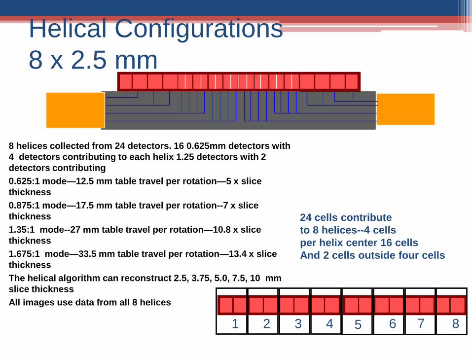
8 x 2.5 mm
24 cells contribute
to 8 helices--4 cells
per helix center 16 cells
And 2 cells outside four cells
1 2 3 4 6 85 7
8 helices collected from 24 detectors. 16 0.625mm detectors with
4 detectors contributing to each helix 1.25 detectors with 2
detectors contributing
0.625:1 mode—12.5 mm table travel per rotation—5 x slice
thickness
0.875:1 mode—17.5 mm table travel per rotation--7 x slice
thickness
1.35:1 mode--27 mm table travel per rotation—10.8 x slice
thickness
1.675:1 mode—33.5 mm table travel per rotation—13.4 x slice
thickness
The helical algorithm can reconstruct 2.5, 3.75, 5.0, 7.5, 10 mm
slice thickness
All images use data from all 8 helices

Helical Interface – 16X ConfigurationsSelect # rows, slice thickness,
pitch and table speed
System displays retrospective
choices based on prospective
detector configuration
• 0.5625:1 5.625 mm/rot = 16 x 0.625 mode
• 0.9375:1 9.375 mm/rot = 16 x 0.625 mode
• 1.375:1 13.75 mm/rot = 16 x 0.625 mode
• 1.75:1 17.5 mm/rot = 16 x 0.625 mode
• 0.6875:1 13.75mm/rot = 16 x 1.25 mode
• 0.9375:1 18.75 mm/rot = 16 x 1.25 mode
• 1.375:1 27.5 mm/rot = 16 x 1.25 mode
• 1.75:1 35 mm/rot = 16 x 1.25 modeTo calculate detector
configuration in
0.5625:1 divide table speed by 9
0.9375:1 divide table speed by 15
1.375:1 divide table speed by 22
1.75:1 divide table speed by 28

Helical Interface – 8X ConfigurationsSelect # rows, slice thickness,
pitch and table speed
System displays retrospective
choices based on prospective
detector configuration
• 0.625:1 6.25 mm/rot = 8 x 1.25 mode
• 0.875:1 8.75 mm/rot = 8 x 1.25 mode
• 1.35:1 13.5 mm/rot = 8 x 1.25 mode
• 1.675:1 16.5 mm/rot = 8 x 1.25 mode
• 0.625:1 12.5mm/rot = 8 x 2.5 mode
• 0.875:1 17.5 mm/rot = 8 x 2.5 mode
• 1.35:1 27.0 mm/rot = 8 x 2.5 mode
• 1.675:1 33.5 mm/rot = 8 x 2.5 mode
To calculate detector
configuration in
0.625:1 divide table speed by 5
0.875:1 divide table speed by 7
1.35:1 divide table speed by 10.8
1.675:1 divide table speed by 13.4
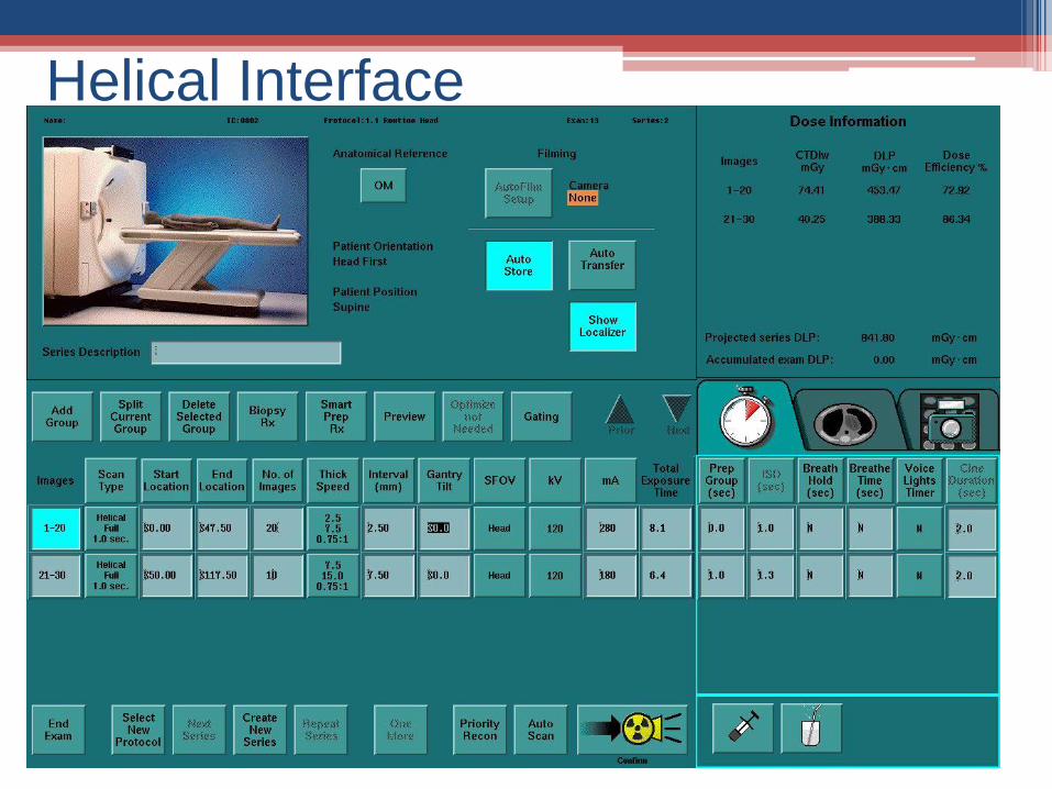
Helical Interface
helical_demo.ppt

Slice Profiles
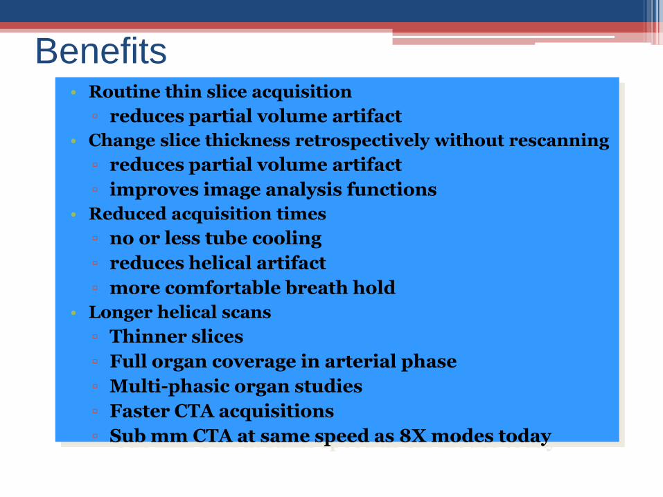
Benefits• Routine thin slice acquisition
▫ reduces partial volume artifact
• Change slice thickness retrospectively without rescanning
▫ reduces partial volume artifact
▫ improves image analysis functions
• Reduced acquisition times
▫ no or less tube cooling
▫ reduces helical artifact
▫ more comfortable breath hold
• Longer helical scans
▫ Thinner slices
▫ Full organ coverage in arterial phase
▫ Multi-phasic organ studies
▫ Faster CTA acquisitions
▫ Sub mm CTA at same speed as 8X modes today
References
• Waterstram-Rich, Christian (2007). Nuclear Medicine and PET/CT. St. Louis, Missouri: Mosby Elsevier.
• Seeram, Euclid (2001). Computed Tomography. USA: W.B. Saunders .