Curve  Fi)ng  

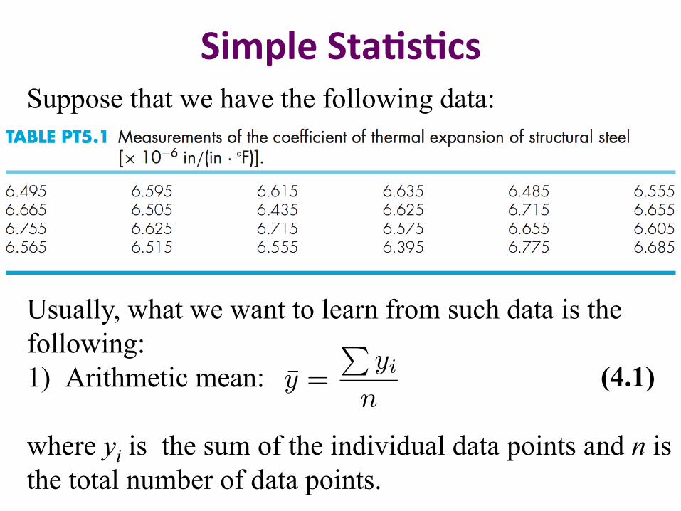
Simple  Sta2s2cs  Suppose that we have the following data:

Usually, what we want to learn from such data is the following: 1)  Arithmetic mean:

where yi is the sum of the individual data points and n is the total number of data points.

y =

Pyin

(4.1)

Simple  Sta2s2cs  

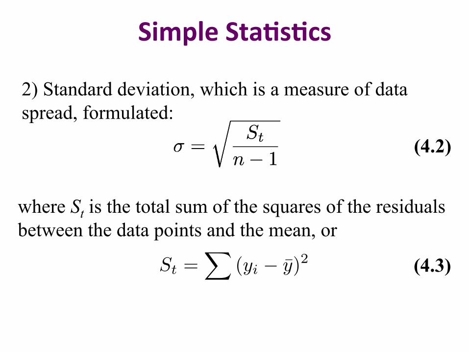
2) Standard deviation, which is a measure of data spread, formulated: where St is the total sum of the squares of the residuals between the data points and the mean, or

St =X

(yi � y)2 (4.3)

(4.2)

Simple  Sta2s2cs  

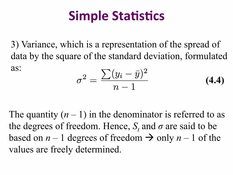
3) Variance, which is a representation of the spread of data by the square of the standard deviation, formulated as: The quantity (n – 1) in the denominator is referred to as the degrees of freedom. Hence, St and σ are said to be based on n – 1 degrees of freedom à only n – 1 of the values are freely determined.

(4.4)

Simple  Sta2s2cs  

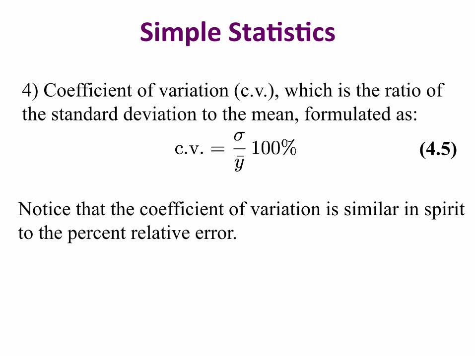
4) Coefficient of variation (c.v.), which is the ratio of the standard deviation to the mean, formulated as: Notice that the coefficient of variation is similar in spirit to the percent relative error.

(4.5)

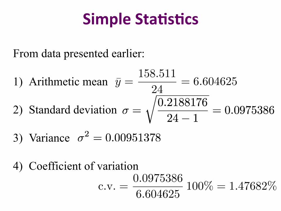
Simple  Sta2s2cs  

From data presented earlier: 1)  Arithmetic mean

2)  Standard deviation 3)  Variance

4)  Coefficient of variation

y =158.511

24= 6.604625

c.v. =0.0975386

6.604625100% = 1.47682%

Normal  Distribu2on  When data is obtained, many times it can considered to be a sample drawn at random from a large population. If the sample number is large, it is theoretically possible to choose class intervals which are very small, but which still have a number of members falling within each class. A frequency polygon of this data has a large number of small line segments and approximates to a continuous curve, which is called a distribution curve. An important symmetrical distribution curve is called the normal curve or normal distribution.

Normal  Distribu2on  Normal distribution curves can differ from one another in the following four ways: 1)  By having different mean values 2)  By having different values of standard deviations 3)  The variables having different values and different

units 4)  By having different areas between the curve and the

horizontal axis.

A normal distribution curve is standardized as follows: (a) The mean value of the unstandardized curve is made the origin, making the mean value

Normal  Distribu2on  (b) The horizontal axis is scaled in standard deviations. This is done by letting where z is called the normal standard variate. (c) The area between the normal curve and the

horizontal axis is made equal to unity.

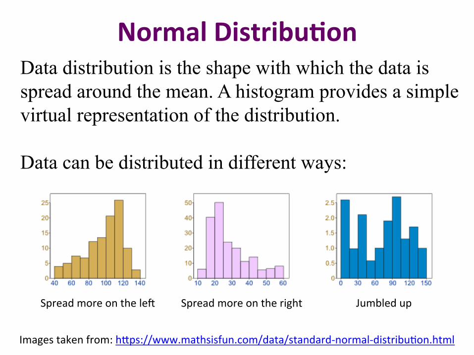
Normal  Distribu2on  Data distribution is the shape with which the data is spread around the mean. A histogram provides a simple virtual representation of the distribution. Data can be distributed in different ways:

Spread  more  on  the  le.   Spread  more  on  the  right   Jumbled  up  

Images  taken  from:  h9ps://www.mathsisfun.com/data/standard-­‐normal-­‐distribu?on.html    

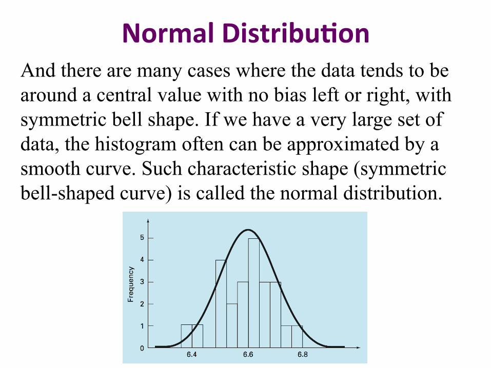
Normal  Distribu2on  And there are many cases where the data tends to be around a central value with no bias left or right, with symmetric bell shape. If we have a very large set of data, the histogram often can be approximated by a smooth curve. Such characteristic shape (symmetric bell-shaped curve) is called the normal distribution.

Normal  Distribu2on  The concepts of the mean, standard deviation, residual sum of the squares, and normal distribution can be used to quantify the confidence that can be ascribed to a particular measurement. If a quantity is normally distributed, the range defined by to will encompass approximately 68% of the total measurements. Similarly, the range defined by to will encompass approximately 95%.

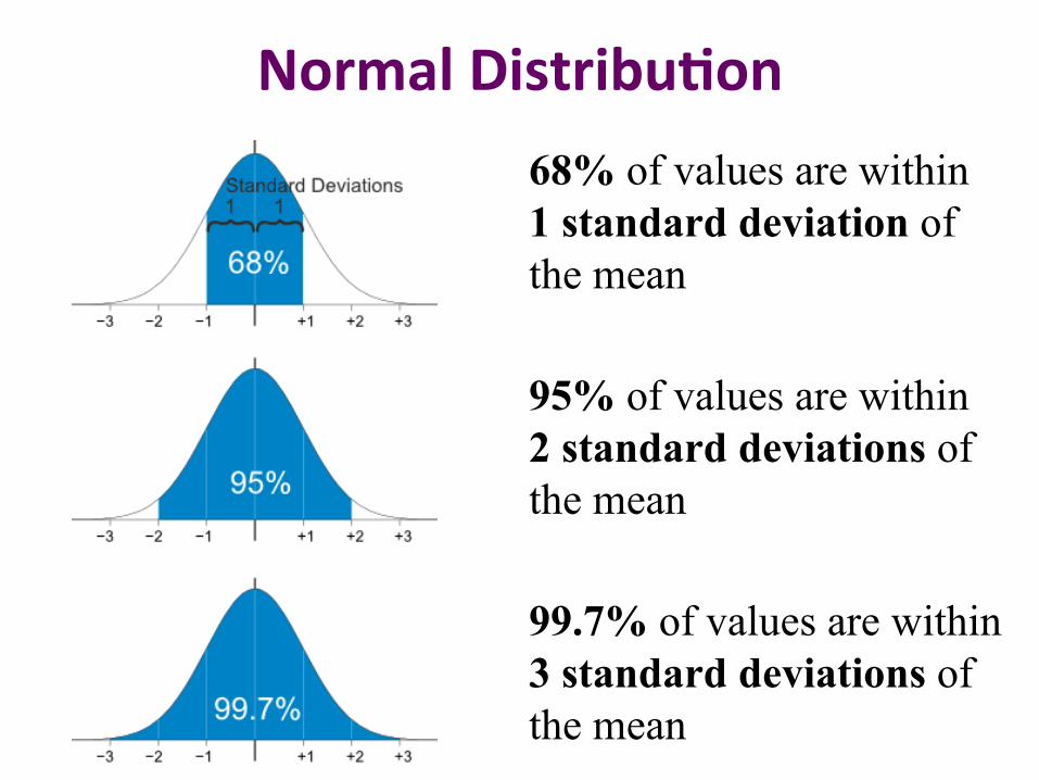
Normal  Distribu2on  68% of values are within 1 standard deviation of the mean 95% of values are within 2 standard deviations of the mean 99.7% of values are within 3 standard deviations of the mean

y � sy

Normal  Distribu2on  From our data, where we can make statement that approximately 95% of the readings should fall between 6.4095 and 6.7997. Or any value is very likely to be within 2 standard deviations.

y = 6.604625

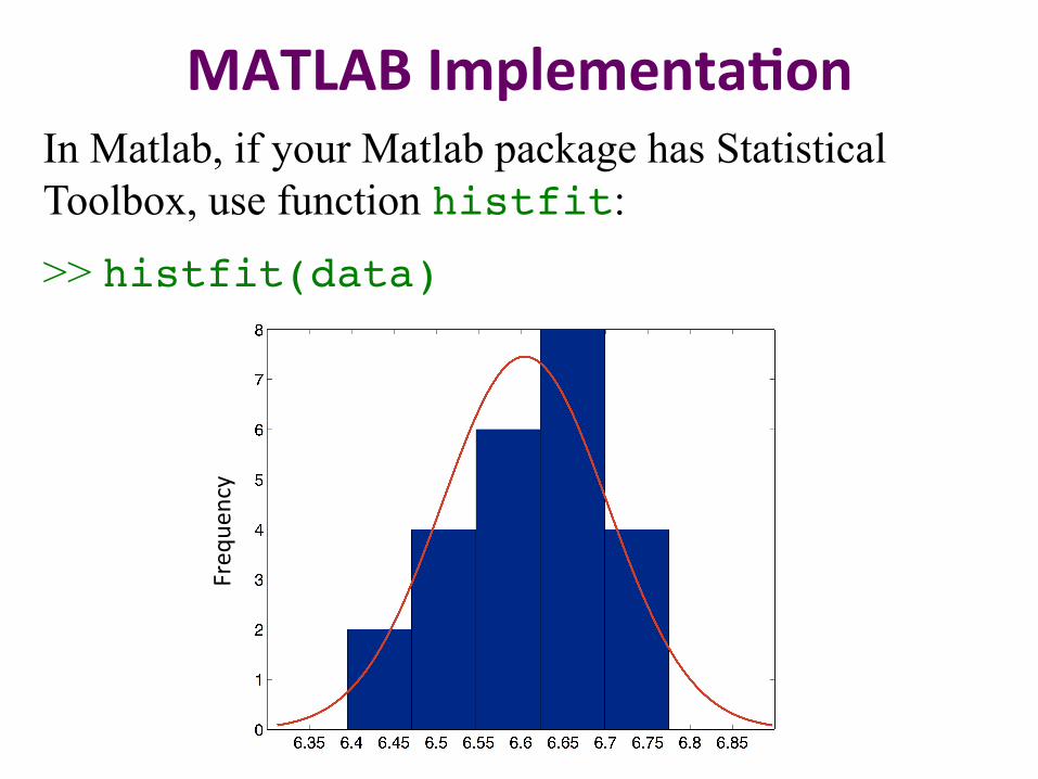
MATLAB  Implementa2on  In Matlab, if your Matlab package has Statistical Toolbox, use function histfit:

>> histfit(data)Freq

uency    

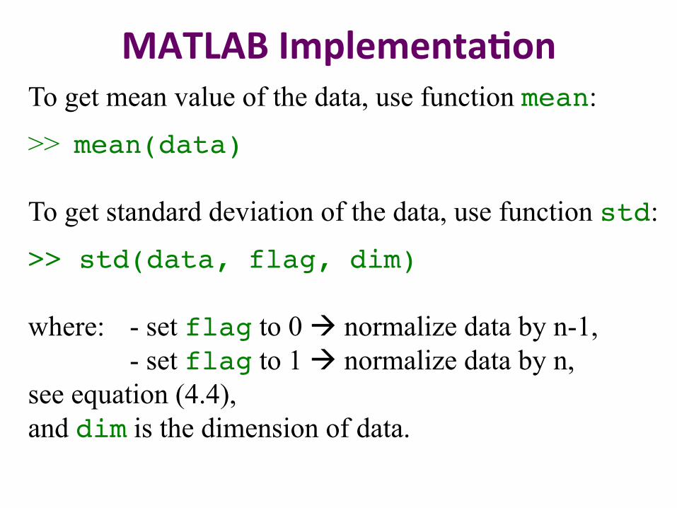
MATLAB  Implementa2on  To get mean value of the data, use function mean:

>> mean(data)

To get standard deviation of the data, use function std:

>> std(data, flag, dim) where: - set flag to 0 à normalize data by n-1,

- set flag to 1 à normalize data by n, see equation (4.4), and dim is the dimension of data.

MATLAB  Implementa2on  Download dataL4.rtf from http://tiny.cc/2vak2x 1)  Calculate mean, standard deviation, variance, and

coefficient of variance 2)  Generate histogram

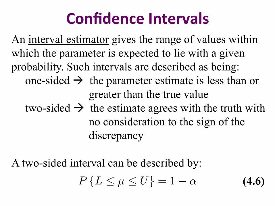
Confidence  Intervals  An interval estimator gives the range of values within which the parameter is expected to lie with a given probability. Such intervals are described as being:

one-sided à the parameter estimate is less than or greater than the true value two-sided à the estimate agrees with the truth with no consideration to the sign of the discrepancy

A two-sided interval can be described by:

P {L µ U} = 1� ↵ (4.6)

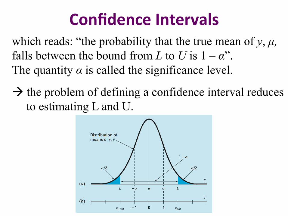
Confidence  Intervals  which reads: “the probability that the true mean of y, µ, falls between the bound from L to U is 1 – α”. The quantity α is called the significance level.

à the problem of defining a confidence interval reduces to estimating L and U.

Confidence  Intervals  Although it is not absolutely necessary, it is customary to view the two-sided interval with the α probability distributed evenly as α/2 in each tail of the distribution, as shown in the figure below.

Confidence  Intervals  If the true variance of the distribution of y, σ2, is known (which is not usually the case), statistical theory states that the sample mean ȳ comes from a normal distribution with mean µ and variance σ2/n. If we don’t know µ, we don’t know where the normal curve is exactly located with respect to ȳ. Hence, we compute a new quantity called the standard normal estimate, represents the normalized distance between ȳ and µ.

z =y � µ

�/pn

(4.7)

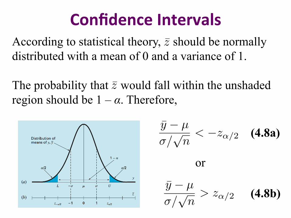
Confidence  Intervals  According to statistical theory, should be normally distributed with a mean of 0 and a variance of 1. The probability that would fall within the unshaded region should be 1 – α. Therefore,

z

z

y � µ

�/pn< �z↵/2

y � µ

�/pn> z↵/2

or

(4.8a)

(4.8b)

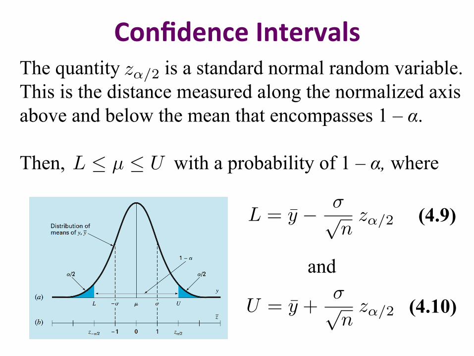
Confidence  Intervals  The quantity is a standard normal random variable. This is the distance measured along the normalized axis above and below the mean that encompasses 1 – α. Then, with a probability of 1 – α, where

and

z↵/2

L µ U

L = y � �pnz↵/2

U = y +�pnz↵/2

(4.9)

(4.10)

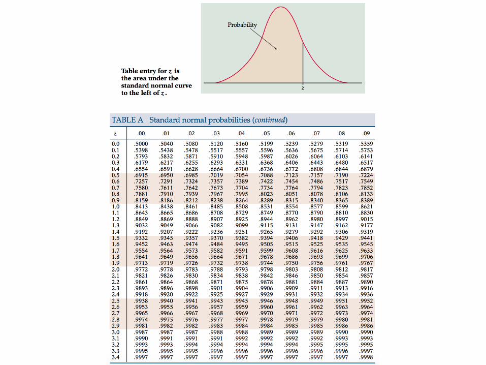
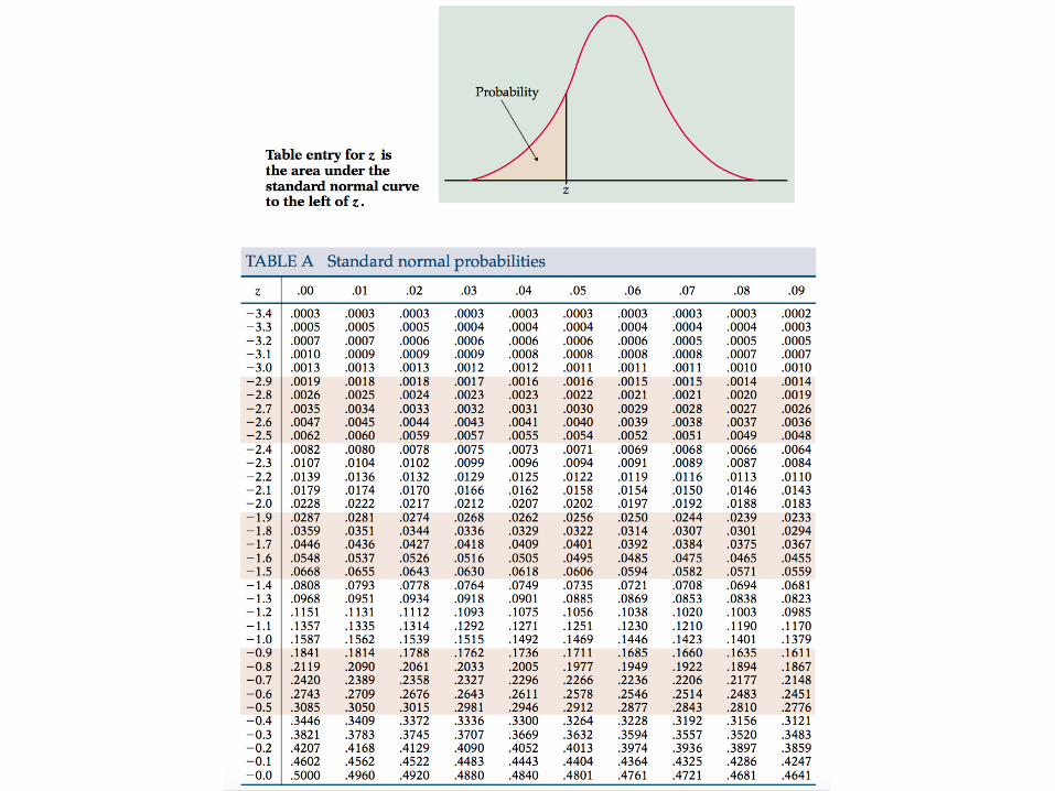
Confidence  Intervals  Values of are tabulated in many resources, such as in statistic books and online resources. Of the online resources are: http://www.stat.purdue.edu/~mccabe/ips4tab/bmtables.pdf (tables presented in the next 2 slides) http://www.normaltable.com http://www.mathsisfun.com/data/standard-normal-distribution-table.html https://en.wikipedia.org/wiki/Standard_normal_table

z↵/2

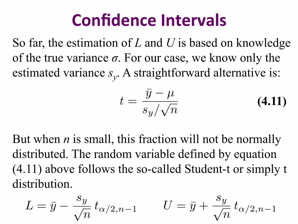
Confidence  Intervals  So far, the estimation of L and U is based on knowledge of the true variance σ. For our case, we know only the estimated variance sy. A straightforward alternative is:

But when n is small, this fraction will not be normally distributed. The random variable defined by equation (4.11) above follows the so-called Student-t or simply t distribution.

t =y � µ

sy/pn

(4.11)

L = y � sypnt↵/2,n�1 U = y +

sypnt↵/2,n�1

Confidence  Intervals  where is the standard random variable for the t distribution for a probability of α/2. The values are also tabulated. See table in the next slide.

t↵/2,n�1

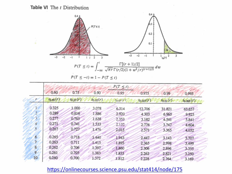
h9ps://onlinecourses.science.psu.edu/stat414/node/175    

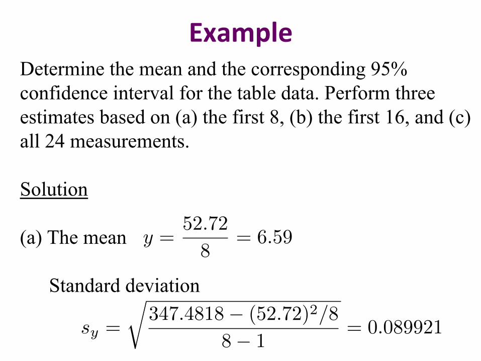
Example  Determine the mean and the corresponding 95% confidence interval for the table data. Perform three estimates based on (a) the first 8, (b) the first 16, and (c) all 24 measurements. Solution (a) The mean

Standard deviation

y =52.72

8= 6.59

sy =

r347.4818� (52.72)2/8

8� 1= 0.089921

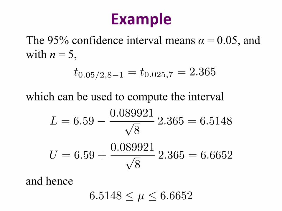
Example   The 95% confidence interval means α = 0.05, and

with n = 5,

which can be used to compute the interval

and hence

t0.05/2,8�1 = t0.025,7 = 2.365

L = 6.59� 0.089921p8

2.365 = 6.5148

U = 6.59 +0.089921p

82.365 = 6.6652

6.5148 µ 6.6652

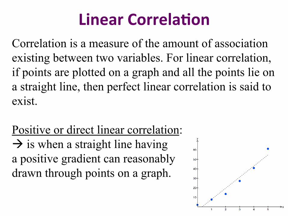
Linear  Correla2on  Correlation is a measure of the amount of association existing between two variables. For linear correlation, if points are plotted on a graph and all the points lie on a straight line, then perfect linear correlation is said to exist. Positive or direct linear correlation: à is when a straight line having a positive gradient can reasonably drawn through points on a graph.

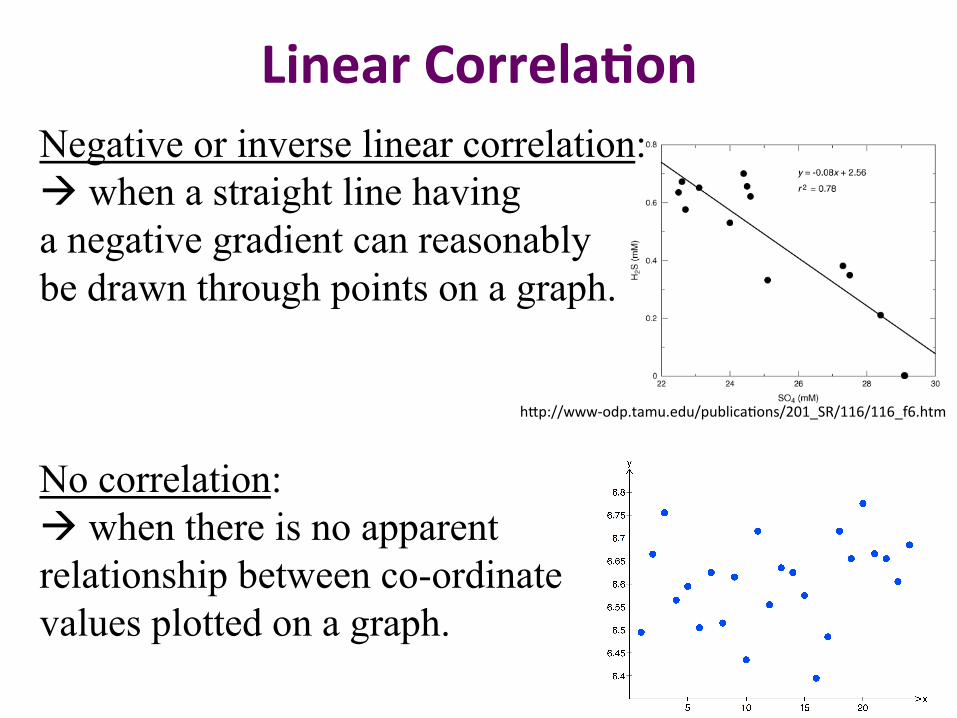
Linear  Correla2on  Negative or inverse linear correlation: à  when a straight line having a negative gradient can reasonably be drawn through points on a graph. No correlation: à when there is no apparent relationship between co-ordinate values plotted on a graph.

h9p://www-­‐odp.tamu.edu/publica?ons/201_SR/116/116_f6.htm  

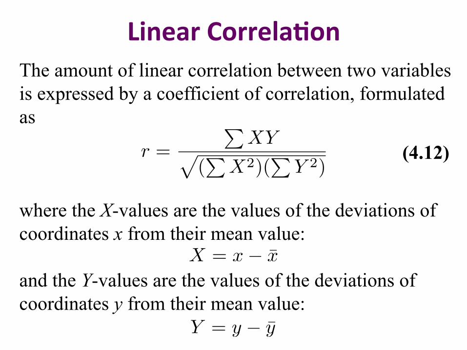
Linear  Correla2on  The amount of linear correlation between two variables is expressed by a coefficient of correlation, formulated as where the X-values are the values of the deviations of coordinates x from their mean value: and the Y-values are the values of the deviations of coordinates y from their mean value:

r =

PXYp

(P

X2)(P

Y 2)

X = x� x

Y = y � y

(4.12)

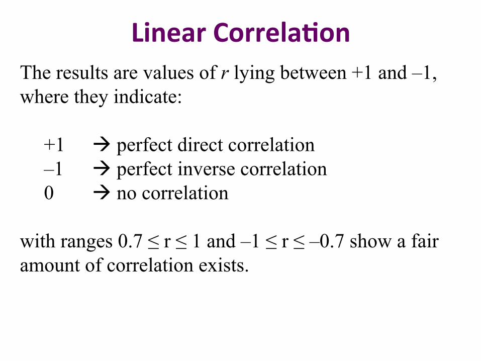
Linear  Correla2on  The results are values of r lying between +1 and –1, where they indicate:

+1 à perfect direct correlation –1 à perfect inverse correlation 0 à no correlation

with ranges 0.7 ≤ r ≤ 1 and –1 ≤ r ≤ –0.7 show a fair amount of correlation exists.

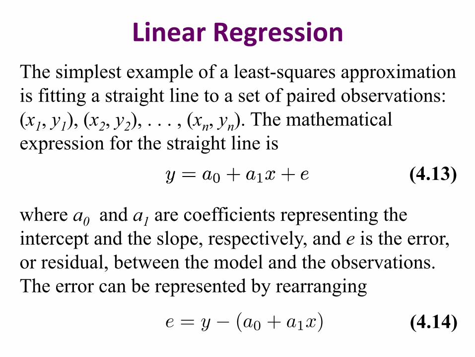
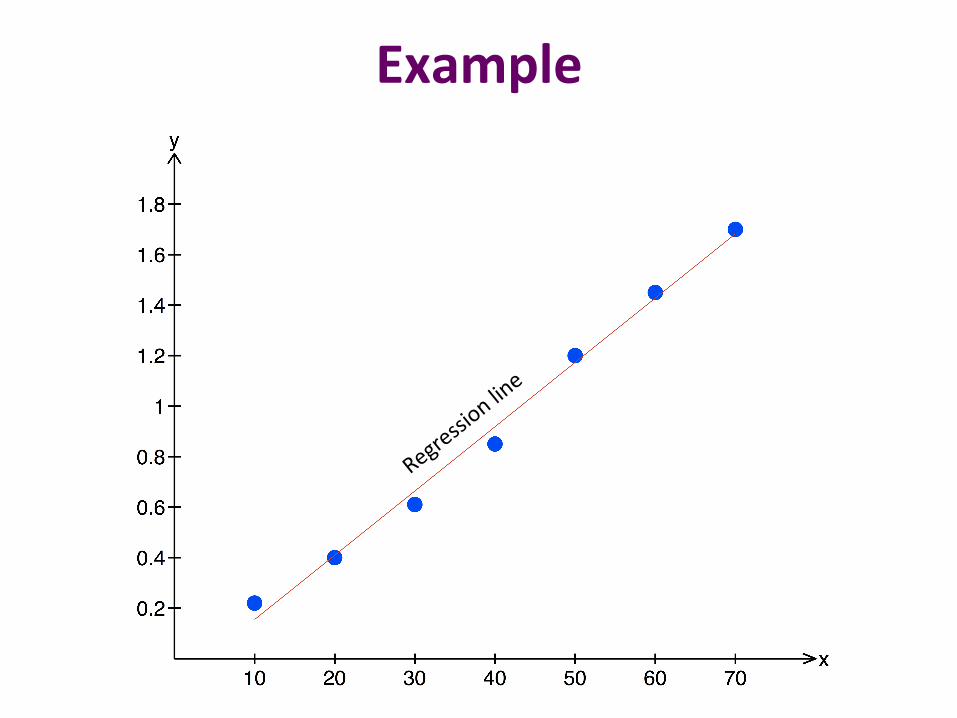
Linear  Regression  The simplest example of a least-squares approximation is fitting a straight line to a set of paired observations: (x1, y1), (x2, y2), . . . , (xn, yn). The mathematical expression for the straight line is where a0 and a1 are coefficients representing the intercept and the slope, respectively, and e is the error, or residual, between the model and the observations. The error can be represented by rearranging

e = y � (a0 + a1x)

(4.13)

(4.14)

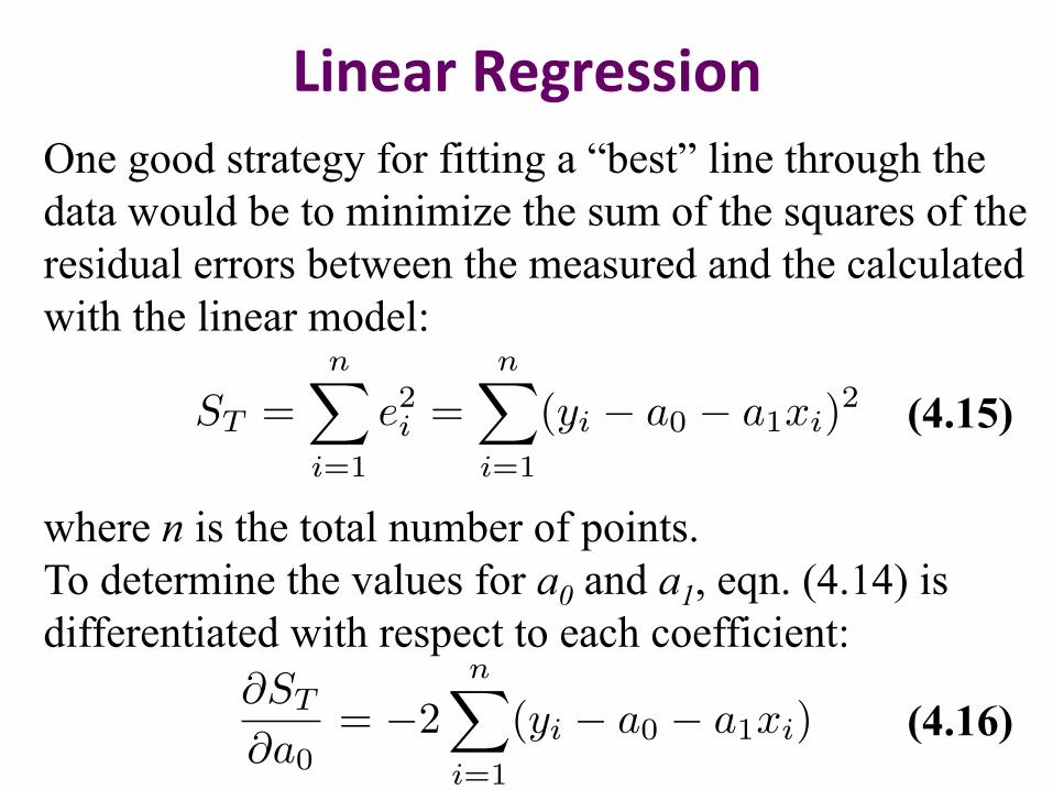
Linear  Regression  One good strategy for fitting a “best” line through the data would be to minimize the sum of the squares of the residual errors between the measured and the calculated with the linear model: where n is the total number of points. To determine the values for a0 and a1, eqn. (4.14) is differentiated with respect to each coefficient:

(4.15) ST =nX

i=1

e

2i =

nX

i=1

(yi � a0 � a1xi)2

@ST

@a0= �2

nX

i=1

(yi � a0 � a1xi) (4.16)

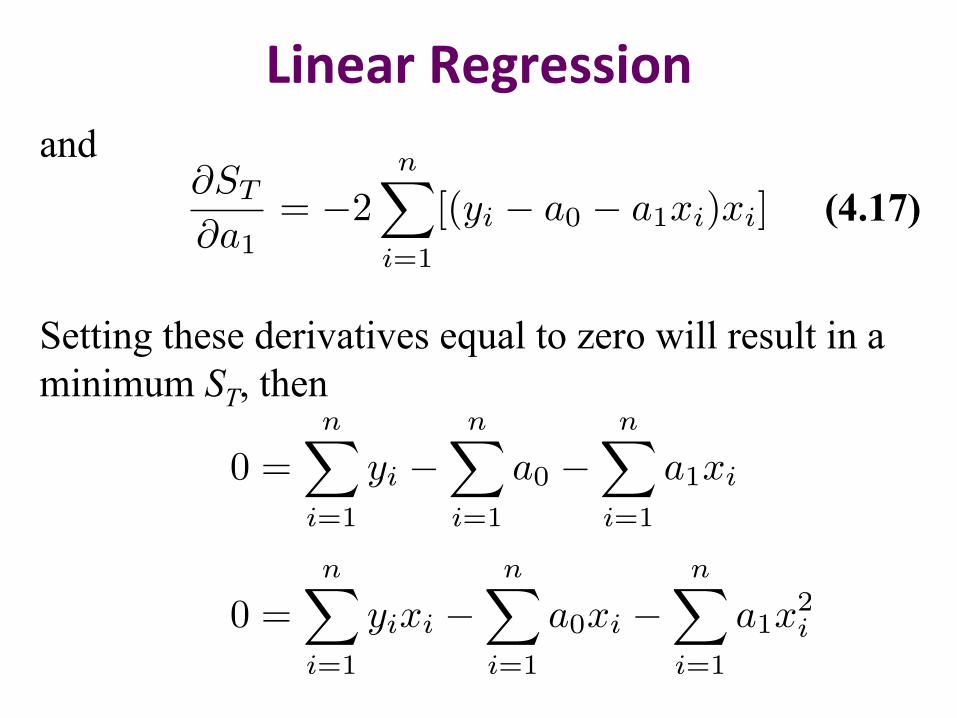
Linear  Regression  and Setting these derivatives equal to zero will result in a minimum ST, then

(4.17) @ST

@a1= �2

nX

i=1

[(yi � a0 � a1xi)xi]

0 =nX

i=1

yi �nX

i=1

a0 �nX

i=1

a1xi

0 =nX

i=1

yixi �nX

i=1

a0xi �nX

i=1

a1x2i

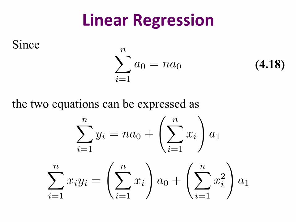
Linear  Regression  Since the two equations can be expressed as

(4.18) nX

i=1

a0 = na0

nX

i=1

yi = na0 +

nX

i=1

xi

!a1

nX

i=1

xiyi =

nX

i=1

xi

!a0 +

nX

i=1

x

2i

!a1

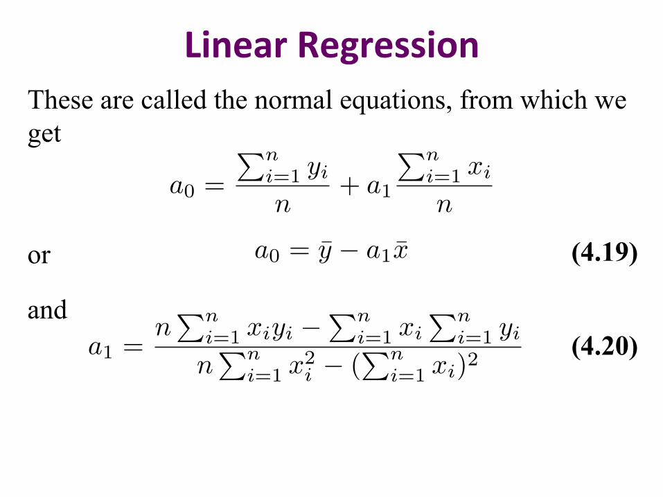
Linear  Regression  These are called the normal equations, from which we get

or

and

(4.19)

a0 =

Pni=1 yi

n

+ a1

Pni=1 xi

n

a1 =n

Pni=1 xiyi �

Pni=1 xi

Pni=1 yi

n

Pni=1 x

2i � (

Pni=1 xi)2

(4.20)

a0 = y � a1x

Example  Consider the following data.

Show if there is correlation and compute the following quantities:

n, x, y

nX

i=1

x

2i ,

nX

i=1

xiyi

nX

i=1

xi,

nX

i=1

yi

a1, a0

10 0.22 20 0.40 30 0.61 40 0.85 50 1.20 60 1.45 70 1.70

x

y

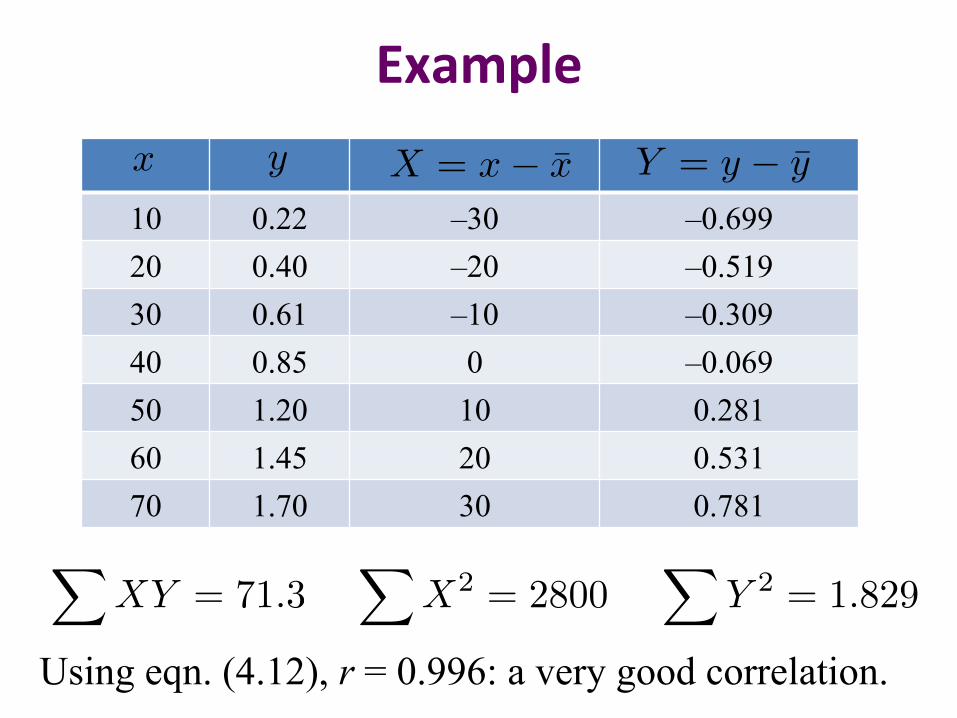
Example  

10 0.22 –30 –0.699 20 0.40 –20 –0.519 30 0.61 –10 –0.309 40 0.85 0 –0.069 50 1.20 10 0.281 60 1.45 20 0.531 70 1.70 30 0.781

X = x� x

Y = y � yx

y

XXY = 71.3

XX2 = 2800

XY 2 = 1.829

Using eqn. (4.12), r = 0.996: a very good correlation.

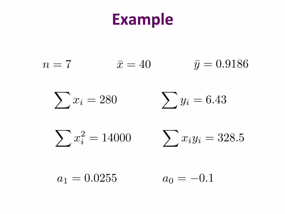
Example  

n = 7 x = 40 y = 0.9186

Xxi = 280

Xyi = 6.43

Xx

2i = 14000

Xxiyi = 328.5

a1 = 0.0255 a0 = �0.1

Example  

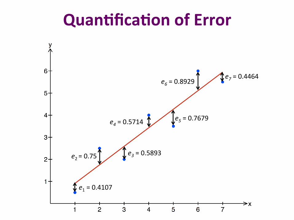
Quan2fica2on  of  Error  

e1  =  0.4107  

e2  =  0.75  e3  =  0.5893  

e5  =  0.7679  

e7  =  0.4464  e6  =  0.8929  

e4  =  0.5714  

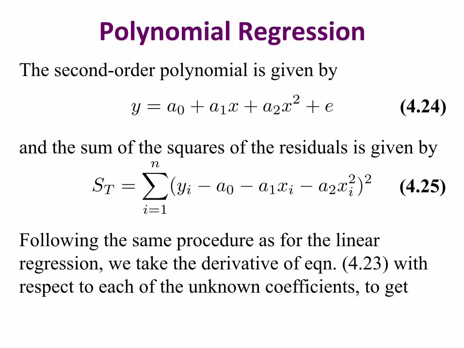
Polynomial  Regression  The second-order polynomial is given by

and the sum of the squares of the residuals is given by Following the same procedure as for the linear regression, we take the derivative of eqn. (4.23) with respect to each of the unknown coefficients, to get

(4.24) y = a0 + a1x+ a2x2 + e

ST =nX

i=1

(yi � a0 � a1xi � a2x2i )

2 (4.25)

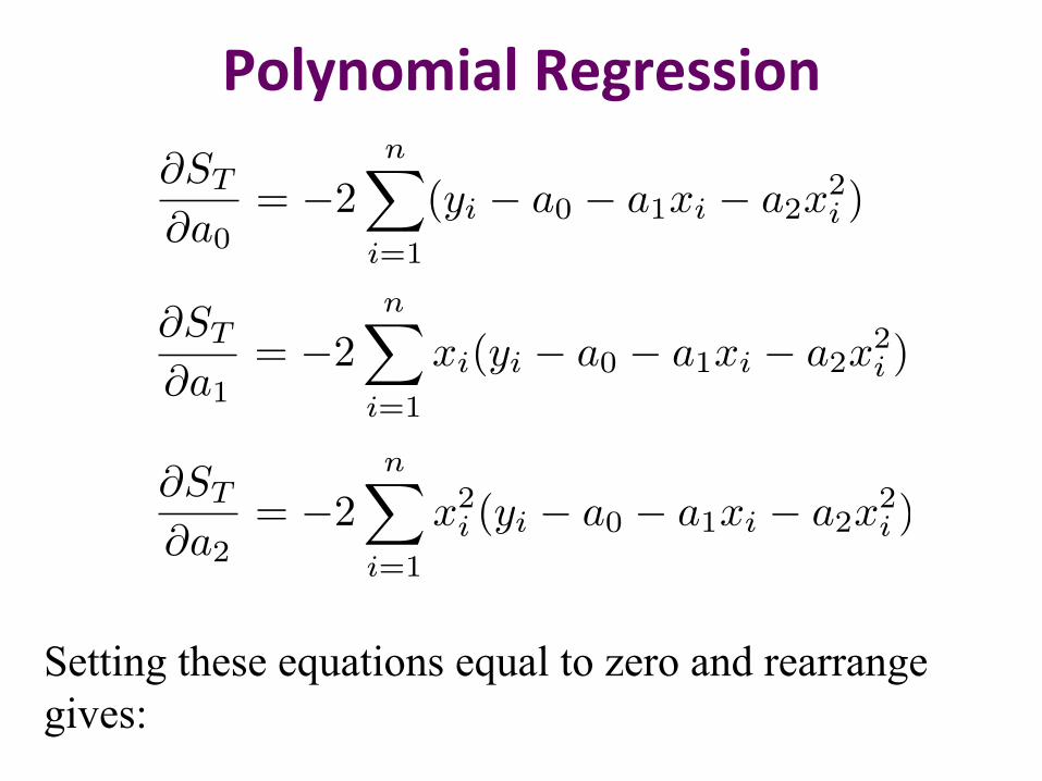
Polynomial  Regression  

Setting these equations equal to zero and rearrange gives:

@ST

@a0= �2

nX

i=1

(yi � a0 � a1xi � a2x2i )

@ST

@a1= �2

nX

i=1

xi(yi � a0 � a1xi � a2x2i )

@ST

@a2= �2

nX

i=1

x

2i (yi � a0 � a1xi � a2x

2i )

Polynomial  Regression  

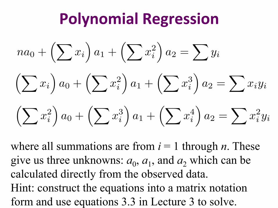
where all summations are from i = 1 through n. These give us three unknowns: a0, a1, and a2 which can be calculated directly from the observed data. Hint: construct the equations into a matrix notation form and use equations 3.3 in Lecture 3 to solve.

na0 +⇣X

xi

⌘a1 +

⇣Xx

2i

⌘a2 =

Xyi

⇣Xxi

⌘a0 +

⇣Xx

2i

⌘a1 +

⇣Xx

3i

⌘a2 =

Xxiyi

⇣Xx

2i

⌘a0 +

⇣Xx

3i

⌘a1 +

⇣Xx

4i

⌘a2 =

Xx

2i yi

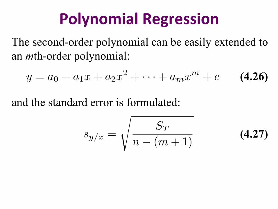
Polynomial  Regression  The second-order polynomial can be easily extended to an mth-order polynomial:

and the standard error is formulated:

(4.26)

(4.27)

y = a0 + a1x+ a2x2 + · · ·+ amx

m + e

sy/x

=

sST

n� (m+ 1)

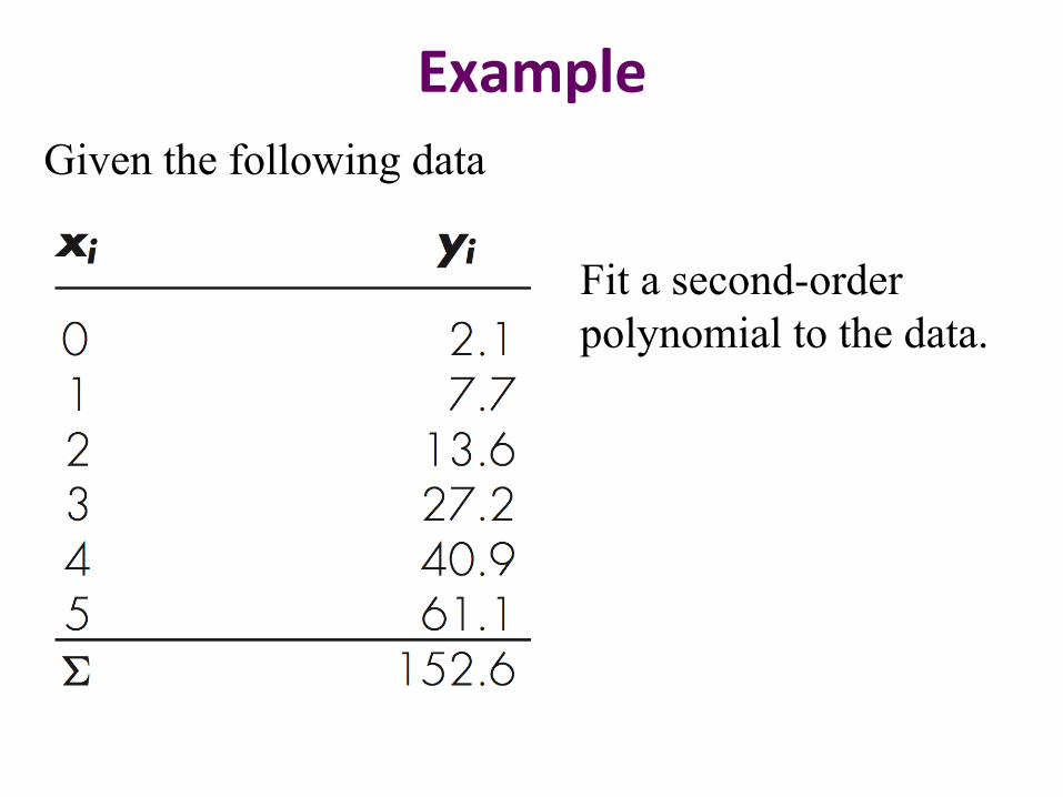
Example  Given the following data

Fit a second-order polynomial to the data.

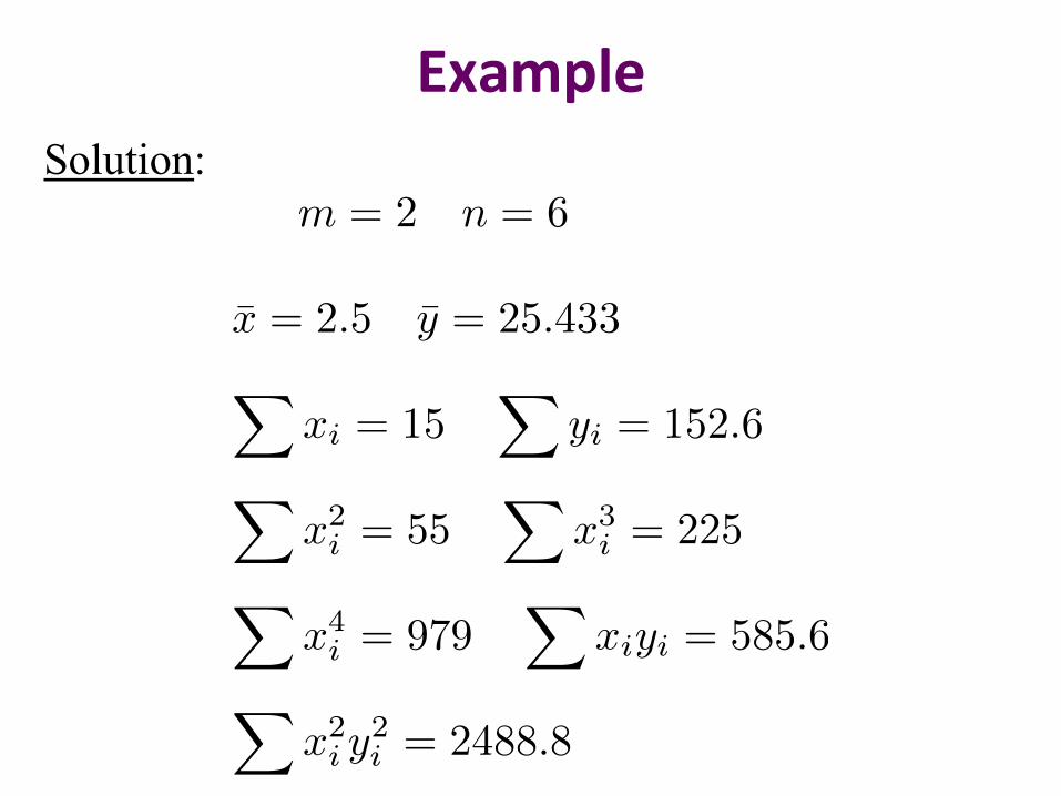
Example  Solution:

m = 2 n = 6

x = 2.5 y = 25.433

Xxi = 15

Xyi = 152.6

Xx

2i = 55

Xx

3i = 225

Xx

4i = 979

Xxiyi = 585.6

Xx

2i y

2i = 2488.8

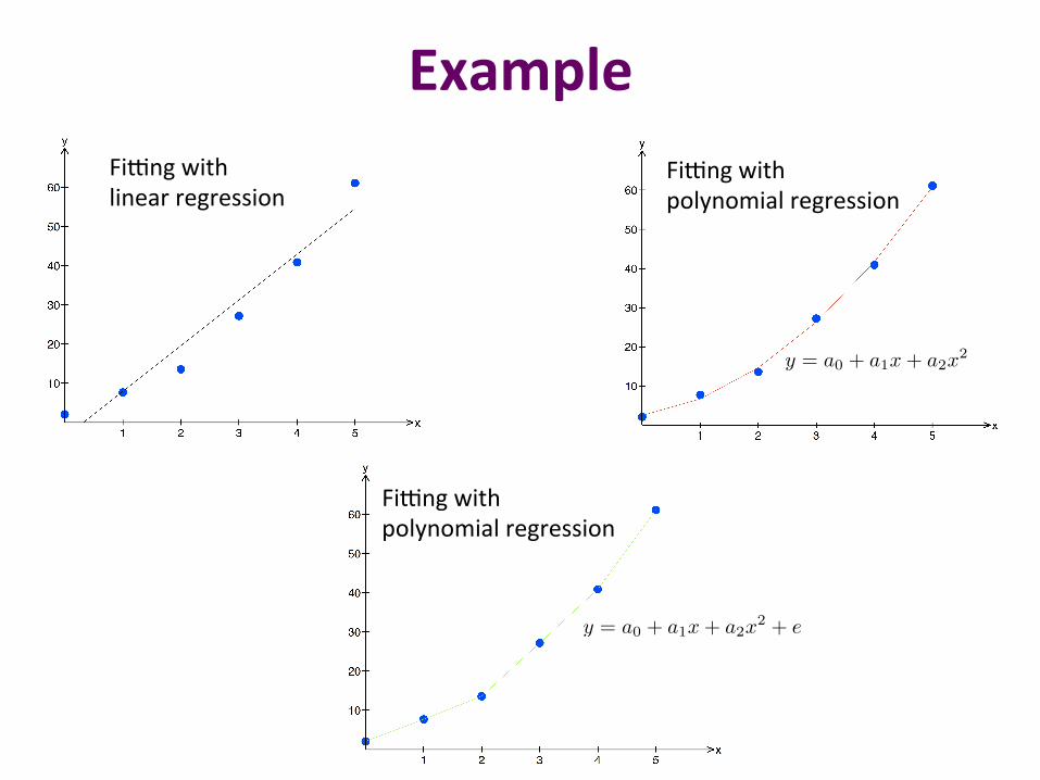
Example  FiPng  with    linear  regression  

FiPng  with    polynomial  regression  

y = a0 + a1x+ a2x2 + e

y = a0 + a1x+ a2x2

FiPng  with    polynomial  regression  

•  Numerical  Methods  for  Engineers,  S.C.  Chapra  and  R.P.  Canale.  

•  Higher  Engineering  Mathema?cs,  John  Bird.  

References