PDEs  Fourier  Series  

Par.al  Differen.al  Equa.ons  (PDEs)  Let the n-dimensional Euclidean space be donated by . A point in has n coordinates . Let u be a function having n coordinates, hence

For n = 2 or n = 3 we may also have different notation, for example:

for functions in for functions in

Sometimes we also write for spherical coordinates. Sometimes we have a “time” coordinate t, in which case for functions in

Par.al  Differen.al  Equa.ons  (PDEs)  There are many different notation for partial derivatives. For example, the partial derivatives of a function in space and time

Physical  Examples  of  PDEs  (1) Wave equation, second-order, linear, homogeneous:

(2) Heat equation, second-order, linear, homogeneous:

(3) Laplace’s equation, second-order, linear, homogeneous:

(4) Poisson’s equation with source function f, second-order, linear, inhomogeneous:

(5) Transport equation, first-order, linear, homogeneous:

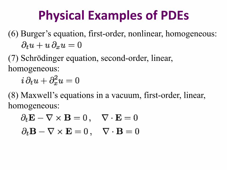
Physical  Examples  of  PDEs  (6) Burger’s equation, first-order, nonlinear, homogeneous:

(7) Schrödinger equation, second-order, linear, homogeneous:

(8) Maxwell’s equations in a vacuum, first-order, linear, homogeneous:

Grad,  Div,  Curl  Define and

Grad,  Div,  Curl  

= Δu (Laplacian)

IBVP  PDEs  PDEs are IBVPs (Initial Boundary Value Problems). Suppose we are interested in studying the diffusion of heat in a body that occupies a bounded region D of x-space. That is, we are interested in solving the heat equation:

in the region:

of (t, x)-space subject to the initial condition:

(13.1)

(13.2)

is temperature distribution at time t = 0.

Boundary  Condi.ons  for  PDEs  Equation (13.2) is a condition on u on the “horizontal” part of the boundary of , but it is not enough to specify u completely; we also need a boundary condition on the “vertical” part of the boundary to tell what happens to the heat when it reaches the boundary surface S of the spatial region D.

(1) One assumption is that S is held at a constant temperature u0, for example by immersing the body in a bath of ice water. This is called Dirichlet condition, where:

(13.3)

Boundary  Condi.ons  for  PDEs  (2) Another assumption is that D is insulated, so that no heat

can flow in or out across S. This is called homogeneous Neumann condition or zero-flux condition. Mathematically, this condition amounts to requiring the normal derivative of u along the boundary S to vanish:

(3) Robin condition is a condition when the region outside D is held at a constant temperature u0, and the rate of heat flow across the boundary S is proportional to the difference in temperatures on the two sides:

(13.5)

(13.4)

Boundary  Condi.ons  for  PDEs  Case (3) is also called Newton’s law of cooling, and a > 0 is the proportionality constant. The conditions (13.3) – (13.4) may be regarded as the limiting case of (13.5) as or

For wave equation, which is second-order in the time variable t,

(13.6)

the conditions required to solve such problem consist of - Initial values of u: - Initial velocity: - Boundary conditions:

Solving  a  Heat/Diffusion  Equa.on  Consider a circular metal rod of length L, insulated along its curved surface so that heat can enter or leave only at the ends. Suppose that both ends are held at temperature zero. The 1-dimensional heat equation with boundary conditions:

Using a method of separation of variables, we try to find solutions of u of the form

(13.9)

and the initial condition

(13.7)

(13.8)

Solving  a  Heat/Diffusion  Equa.on  If we substitute into (13.7) we obtain

Now the left side depends only on t, whereas the right side depends only on x. Since they are equal, they both must be equal to a constant A:

The variables in (13.10) may be separated by dividing both sides by yielding

(13.10)

(13.11)

Solving  a  Heat/Diffusion  Equa.on  These are simple ODEs for T and X that can be solved by elementary methods. (1) If A is positive, the general solutions of the equations for

T and X are

where

(13.13a)

(2) If A is negative, the general solutions of the equations for T and X are

(13.12a)

(13.12b)

(13.13b)

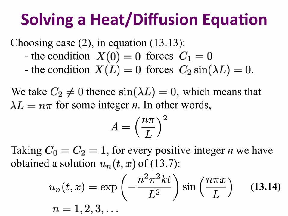
Solving  a  Heat/Diffusion  Equa.on  Choosing case (2), in equation (13.13):

- the condition forces - the condition forces

Taking for every positive integer n we have obtained a solution of (13.7):

(13.14)

We take thence which means that for some integer n. In other words,

Solving  a  Heat/Diffusion  Equa.on  We obtain more solutions by taking linear combinations of the un’s, and then passing to infinite linear combinations, where the solutions now

Applying the initial condition in (13.8) to (13.15) we get

(13.16)

(13.15)

Solving  a  Heat/Diffusion  Equa.on  If we consider other boundary conditions, such as zero-flux condition, the problem now becomes

We use the same technique as before, but the conditions in (13.11) are replaced by

(13.18)

(13.17)

Differentiating (13.13b) and plugging the conditions:

Solving  a  Heat/Diffusion  Equa.on  From which we obtain the sequence of solutions

(13.20)

(13.19)

which can be combined to form the series

Example  Solve the following 1D heat/diffusion equation

(13.21)

Solution: We use the results described in equation (13.19) for the heat equation with homogeneous Neumann boundary condition as in (13.17). From where , we get Applying equation (13.20) we obtain the general solution

Example  From the initial condition

and from matching with the initial condition, we get

Substituting these into the general solution, we obtain the particular solution:

Example  Analytical Solution MATLAB’s pdepe function

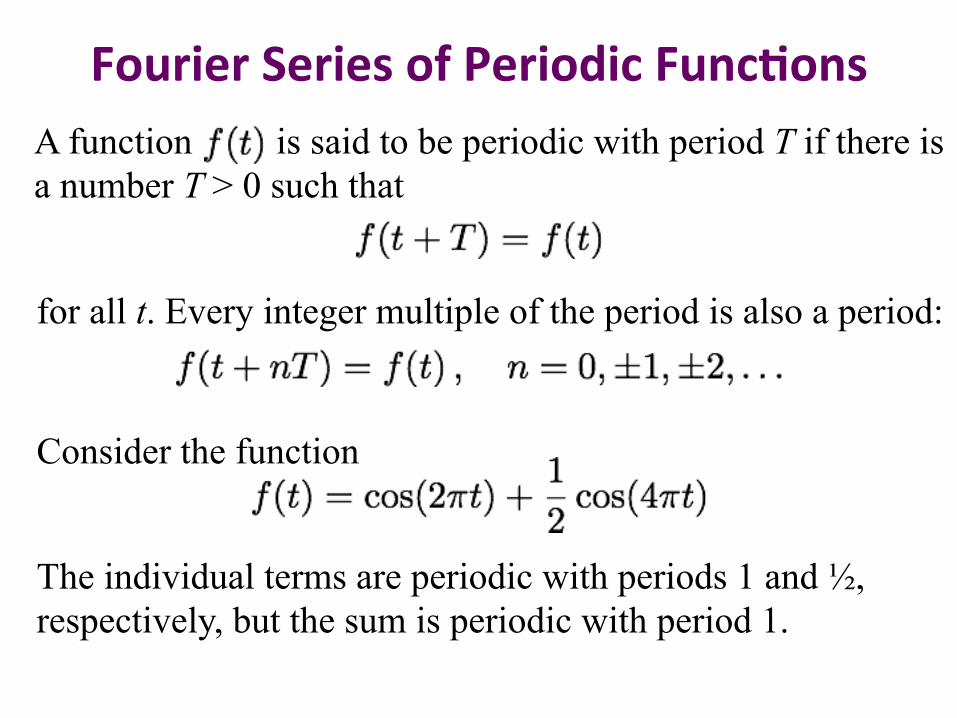
Fourier  Series  of  Periodic  Func.ons  A function is said to be periodic with period T if there is a number T > 0 such that

for all t. Every integer multiple of the period is also a period:

Consider the function

The individual terms are periodic with periods 1 and ½, respectively, but the sum is periodic with period 1.

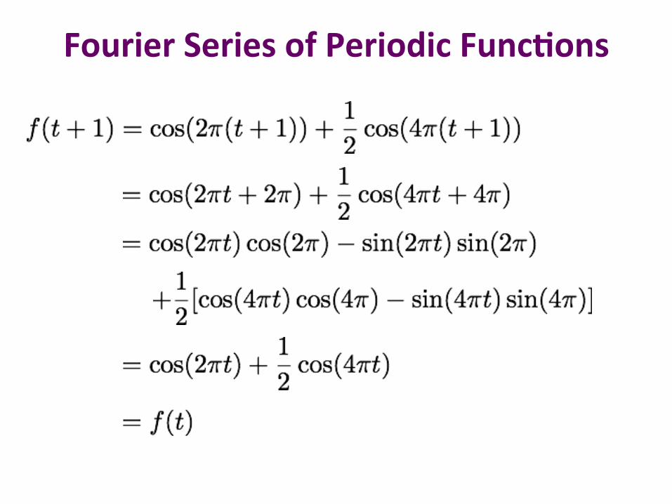
Fourier  Series  of  Periodic  Func.ons  

Fourier  Series  of  Periodic  Func.ons  Suppose that is a function defined on the real line such that for all t. Such functions are said to be periodic with period T, or T-periodic. A continuous Fourier series of a function with period T can be written:

(13.21)

or more concisely,

where is called the fundamental frequency and its constant multiples etc are called harmonics.

Fourier  Series  of  Periodic  Func.ons  Recall the formulas

Hence

Also the formulas

Fourier  Series  of  Periodic  Func.ons  The series in (13.21) can be rewritten as

(13.22)

Now, letting

Fourier  Series  of  Periodic  Func.ons  The expression for becomes

The coefficients cn are complex numbers and they satisfy

Notice that when n = 0 we have which implies that c0 is a real number.

For any value of n, the magnitudes of cn and c−n are equal:

Fourier  Series  of  Periodic  Func.ons  Then the series

(13.23)

can be written as

where, they are both called the Fourier series of f.

Fourier  Series  of  Periodic  Func.ons  How can the coefficients be calculated in terms of ? Let us multiply both sides of (13.22) by (k being an integer) and integrate from 0 to T:

If , the integral term on the right hand side:

Fourier  Series  of  Periodic  Func.ons  

and the case if n = k:

Fourier  Series  of  Periodic  Func.ons  Hence, the only term in the series that survives the integration is the term with n = k, and we obtain

(13.24)

In other words, relabeling the integer k as n, we have the formula for the coefficients cn:

which are the coefficients for the series in (13.23). It is then straightforward to find the coefficients if the series is in the form expressed in (13.21).

Fourier  Series  of  Periodic  Func.ons  From the expressions in (13.22) where

(13.25)

and for

(13.26)

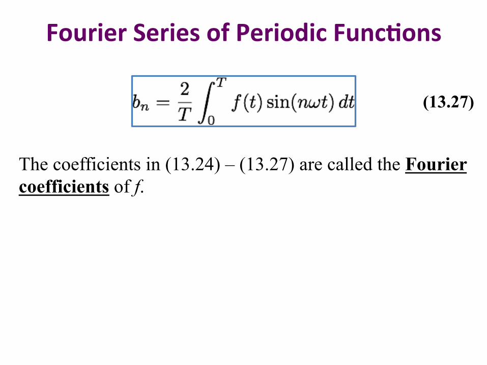
Fourier  Series  of  Periodic  Func.ons  

The coefficients in (13.24) – (13.27) are called the Fourier coefficients of f.

(13.27)

Fourier  Series  of  Periodic  Func.ons  A useful observation is

Function F is even if F(-x) = F(x) and odd if F(-x) = -F(x).

Since is even and is odd, we have:

if f is even:

if f is odd:

Example  Use the (continuous) Fourier series to approximate the square or rectangular wave function

Solution: We first calculate

Example  Then the coefficient an:

Solving term by term:

Example  

from which, the solutions for each sequence:

Example  The middle term gives

Checking the solutions for each n:

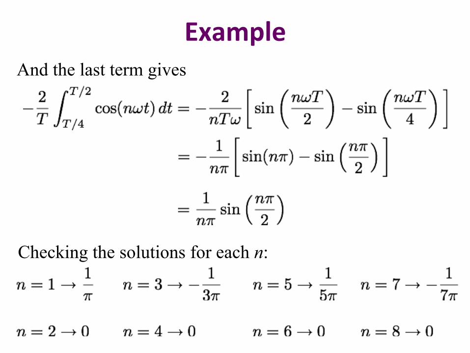
Example  And the last term gives

Checking the solutions for each n:

Example  Collecting all solutions from all terms gives us

etc.

Example  In general

Similarly, it can be determined that all the b’s = 0. Therefore the Fourier series approximation is

Example  

Fourier  Integral  and  Transform  Fourier integral is a tool used to analyze non-periodic waveforms or non-recurring signals, such as lightning bolts. Fourier integral formula is derived from Fourier series by allowing the period to approach infinity:

(13.28)

where the coefficients become a continuous function of the frequency variable ω, as in

(13.29)

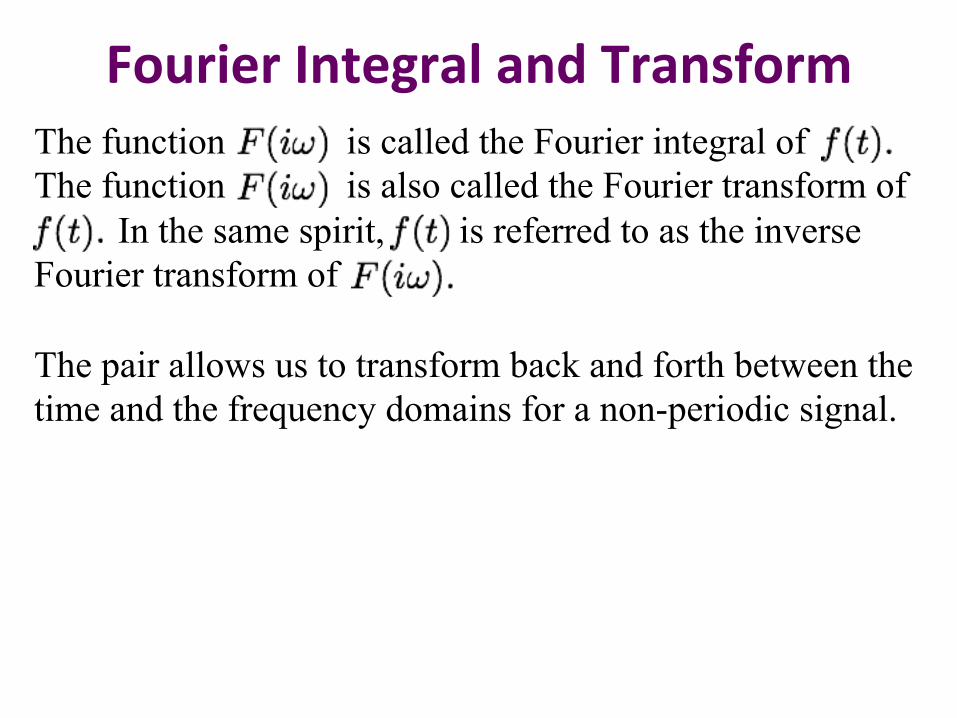
Fourier  Integral  and  Transform  The function is called the Fourier integral of The function is also called the Fourier transform of In the same spirit, is referred to as the inverse Fourier transform of The pair allows us to transform back and forth between the time and the frequency domains for a non-periodic signal.

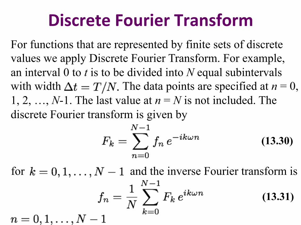
Discrete  Fourier  Transform  For functions that are represented by finite sets of discrete values we apply Discrete Fourier Transform. For example, an interval 0 to t is to be divided into N equal subintervals with width The data points are specified at n = 0, 1, 2, …, N-1. The last value at n = N is not included. The discrete Fourier transform is given by

(13.30)

for and the inverse Fourier transform is

(13.31)

References  1) Fourier Analysis and Its Applications, Gerald B. Folland