Finite  Difference  Methods    (FDMs)  3  

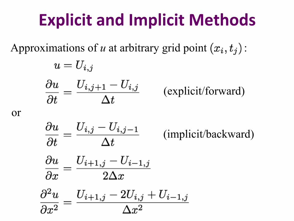
Explicit  and  Implicit  Methods  Approximations of u at arbitrary grid point :

or

(explicit/forward)

(implicit/backward)

Crank-­‐Nicolson  Method  Approximations of u and its derivatives:

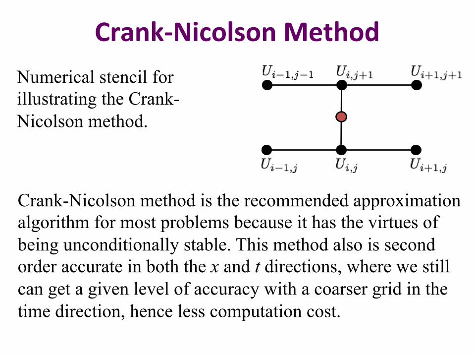
Crank-­‐Nicolson  Method  Numerical stencil for illustrating the Crank-Nicolson method.

Crank-Nicolson method is the recommended approximation algorithm for most problems because it has the virtues of being unconditionally stable. This method also is second order accurate in both the x and t directions, where we still can get a given level of accuracy with a coarser grid in the time direction, hence less computation cost.

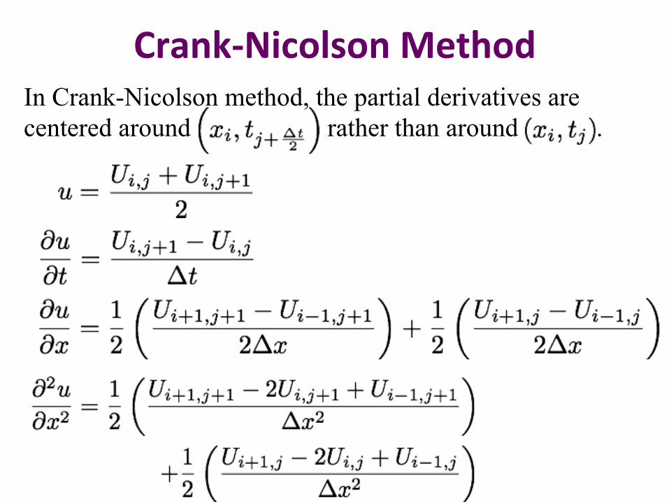
Crank-­‐Nicolson  Method  In Crank-Nicolson method, the partial derivatives are centered around rather than around .

Crank-­‐Nicolson  Method  

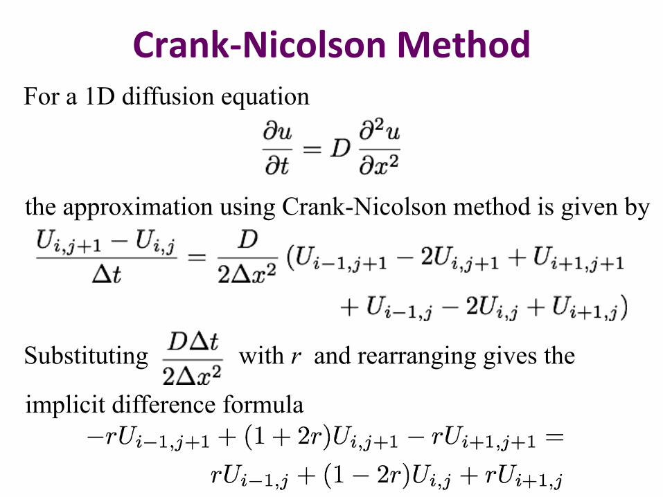
the approximation using Crank-Nicolson method is given by

For a 1D diffusion equation

implicit difference formula

Substituting with r and rearranging gives the

Crank-­‐Nicolson  Method  

, the difference formula is given by If Neumann BC is imposed along x = 0 where

If Neumann BC is imposed along x = L or at i = M, where , the difference formula is given by

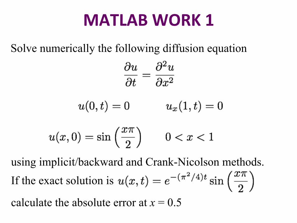
MATLAB  WORK  1  Solve numerically the following diffusion equation

using implicit/backward and Crank-Nicolson methods. If the exact solution is

calculate the absolute error at x = 0.5

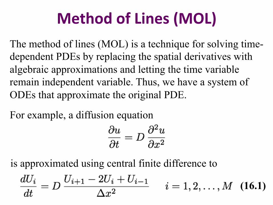
Method  of  Lines  (MOL)  The method of lines (MOL) is a technique for solving time-dependent PDEs by replacing the spatial derivatives with algebraic approximations and letting the time variable remain independent variable. Thus, we have a system of ODEs that approximate the original PDE.

(16.1)

For example, a diffusion equation

is approximated using central finite difference to

Method  of  Lines  (MOL)  If Dirichlet BC is imposed at x = 0, where , then

Therefore the ODE of equation (16.1) for i = 1 is not required and the ODE for i = 2 becomes

At i = M, we have

The value at i = M+1 is obtain from the boundary.

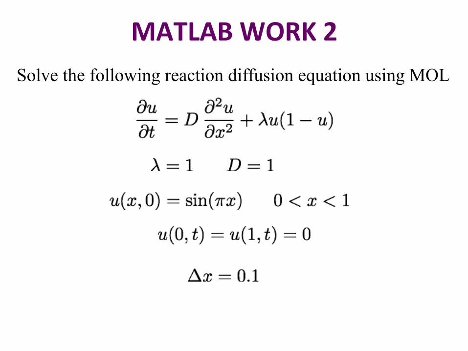
MATLAB  WORK  2  Solve the following reaction diffusion equation using MOL

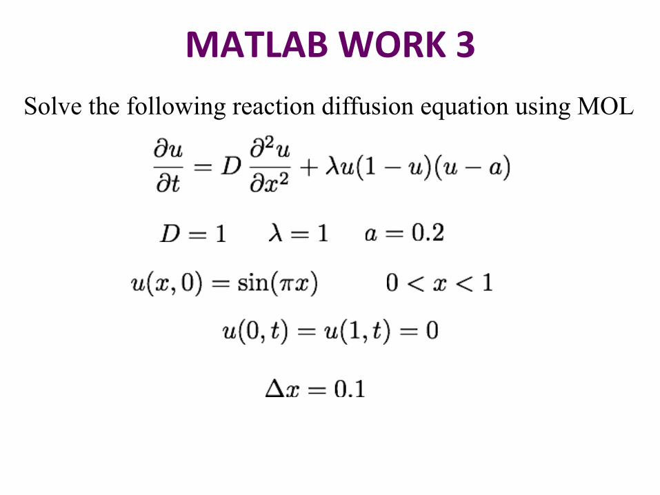
MATLAB  WORK  3  Solve the following reaction diffusion equation using MOL

Crank-­‐Nicolson  Method  http://www.dynamicearth.de/compgeo/ http://www.scholarpedia.org/article/Method_of_lines