CYBER HAGGLER: WEB BASED BARGAINING USING GENETIC ALGORITHM

by

KUMAR UJJWAL

(Under the Direction of Jay E. Aronson)

ABSTRACT

In this thesis, we analyze the sequential bargaining problem from a different perspective. Instead

of taking a game theoretic approach, we model bargaining as a search problem and use a genetic

algorithm to find an equilibrium outcome. Users, as buyers or sellers, only have to specify the product

details and reservation price. The bargaining process is done by buyer and seller software agents. We

have also developed a fully functional website Cyber Haggler (http://www.cyberhaggler.com) to illustrate

our concepts. The software agents are based on realistic assumptions of bounded rationality and they learn

from trial-and-error over time. We also compare Cyber Haggler to both Kasbah and EBay.com. Results

show that our model can be easily implemented commercially on the Internet. Thus, we have been

successful in modeling real world human-like bargaining on the Internet.

INDEX WORDS: Genetic Algorithm, Software Agents, Bargaining Problem, Economic Equilibrium, Bounded Rationality

CYBER HAGGLER: WEB BASED BARGAINING USING GENETIC ALGORITHM

by

KUMAR UJJWAL

B.Tech, ABV-IIITM, India, 2005

M.Tech, ABV-IIITM, India, 2005

A Thesis Submitted to the Graduate Faculty of The University of Georgia in Partial Fulfillment of the

Requirements for the Degree

MASTER OF SCIENCE

ATHENS, GEORGIA

2007

© 2007

Kumar Ujjwal

All Rights Reserved

CYBER HAGGLER: WEB BASED BARGAINING USING GENETIC ALGORITHM

by

KUMAR UJJWAL

Major Professor: Dr. Jay E. Aronson

Committee: Dr. Walter D. PotterDr. Khaled Rasheed

Electronic Version Approved:

Maureen GrassoDean of the Graduate SchoolThe University of GeorgiaMay 2007

iv

DEDICATION

This thesis is dedicated to my adorable mom and doting dad.

v

ACKNOWLEDGEMENTS

I would like to thank Dr. Jay Aronson for numerous fruitful discussions, constructive criticisms and

wonderful ideas. I would like to thank Dr. Don Potter and Dr. Khaled Rasheed for being in my committee

and for their constant support and encouragement during the development of the thesis work. I would like

to thank my wonderful friend Colin Nicholson for going through the whole manuscript and fixing the

grammatical errors.

vi

TABLE OF CONTENTS

Page

ACKNOWLEDGEMENTS.......................................................................................................................... v

LIST OF TABLES.....................................................................................................................................viii

LIST OF FIGURES ..................................................................................................................................... ix

CHAPTER

1 INTRODUCTION..................................................................................................................... 1

1.1 BARGAINING THEORY.............................................................................................. 1

1.2 GAME THEORY AND THE NASH EQUILIBRIUM.................................................. 2

1.3 PERFECT RATIONALITY VS. BOUNDED RATIONALITY ................................... 5

1.4 E-COMMERCE 2007: AUCTION VS. BARGAINING ............................................... 5

1.5 CYBER HAGGLER: AN INTRODUCTION................................................................ 6

2 ONLINE BARGAINING: STATE OF THE ART ................................................................... 8

2.1 THE KASBAH OPEN MARKETPLACE..................................................................... 8

2.2 RELEVANT EVOLUTIONARY ALGORITHM MODELS ...................................... 9

2.3 BAZAAR...................................................................................................................... 10

3 CYBER HAGGLER: WEB BASED BARGAINING VIA A GENETIC ALGORITHM ..... 12

3.1 GENETIC ALGORITHM ............................................................................................ 12

3.2 BARGAINING AS A SEARCH PROBLEM .............................................................. 12

3.3. THE BARGAINING MODEL.................................................................................... 13

3.4 GENETIC ALGORITHM DESIGN FOR CYBER HAGGLER ................................. 18

3.5 USER INTERFACE ..................................................................................................... 23

vii

3.6 CYBER HAGGLER VS. KASBAH ............................................................................ 27

3.7 CYBER HAGGLER VS. EBAY.................................................................................. 28

4 EXPERIMENTS AND RESULTS.......................................................................................... 30

4.1 EXPERIMENT 1.......................................................................................................... 30

4.2 EXPERIMENT 2.......................................................................................................... 37

4.3 EXPERIMENT 3.......................................................................................................... 39

4.4 EXPERIMENT 4.......................................................................................................... 40

4.5 EXPERIMENT 5.......................................................................................................... 42

5 CONCLUSION ....................................................................................................................... 44

5.1 INTRODUCTION........................................................................................................ 44

5.2 SUMMARY ................................................................................................................. 44

5.3 FUTURE WORK ......................................................................................................... 45

REFERENCES .......................................................................................................................................... 47

viii

LIST OF TABLES

Page

Table 3.1: A SAMPLE INITIAL BUYER POPULATION........................................................................ 19

Table 3.2: A SAMPLE INITIAL SELLER POPULATION ...................................................................... 20

Table 3.3: COMPARISON OF CYBER HAGGLER AND KASBAH...................................................... 28

Table 3.4: COMPARISON OF CYBER HAGGLER AND EBAY ........................................................... 29

ix

LIST OF FIGURES

Page

Figure 1.1: Bargaining Process ..................................................................................................................... 1

Figure 3.1: A buyer makes his offers starting from the seller’s reservation price (RPs) ........................... 14

Figure 3.2: A seller makes his offers starting from the buyer’s reservation price (RPb). .......................... 14

Figure 3.3: Buyer’s strategy for different values of Psi (ψ)........................................................................ 16

Figure 3.4: Design overview of Cyber Haggler.......................................................................................... 21

Figure 3.5: Cyber Haggler Form for selling a digital camera ..................................................................... 23

Figure 3.6: A successful product submission in Cyber Haggler’s database ............................................... 24

Figure 3.7: Cyber Haggler buyer form........................................................................................................ 25

Figure 3.8: Cyber Haggler buyer’s search result ........................................................................................ 26

Figure 3.9: A successful deal at $113 when RPs=80 and RPb=120 .......................................................... 27

Figure 4.1: Effect of varying population size where Pc = 80%, Pm =0.005, selection method=roulette

wheel, number of generations=40, elitism =false ..................................................................... 32

Figure 4.2: Comparison of Deal Price using roulette wheel selection and Tournament Selection with

tournament size of 2.................................................................................................................. 33

Figure 4.3: Effect of varying crossover rate where N=20, Pm =0.005, selection method=roulette wheel,

number of generations=40, elitism =false, seller’s deadline (Ts) > buyer’s deadline (Tb)........ 33

Figure 4.4: Effect of varying crossover rate where N=20, Pm =0.005, selection method=roulette wheel,

number of generations=40, elitism =false, buyer’s deadline (Tb) > seller’s deadline (Ts)........ 34

Figure 4.5: Effect of varying mutation rate where N=20, Pc =80%, selection method=roulette wheel,

number of generations=40, elitism =false, seller’s deadline (Ts) > buyer’s deadline (Tb)........ 35

x

Figure 4.6: Effect of varying mutation rate where N=20, Pc =80%, selection method=roulette wheel,

number of generations=40, elitism =false, seller’s deadline (Ts) < buyer’s deadline (Tb)........ 35

Figure 4.7: One-to-one bargaining game with RPb=130, RPs=80, Tb=10 and Ts=20 ................................. 36

Figure 4.8: Result of ten runs of one-to-one bargaining game described in Figure 4.7.............................. 36

Figure 4.9: One-to-one bargaining game with RPb=130, RPs=80, Tb=10 and Ts=50 using random search

.................................................................................................................................................................... 37

Figure 4.10: One-to-one bargaining game with RPb=130, RPs=80, Tb=10 and Ts=50 using genetic

algorithm................................................................................................................................... 38

Figure 4.11: One-to-one bargaining game with RPb=130, RPs=80, Tb=50 and Ts=10 using random search

.................................................................................................................................................................... 38

Figure 4.12: One-to-one bargaining game with RPb=130, RPs=80, Tb=50 and Ts=10 using genetic

algorithm................................................................................................................................... 39

Figure 4.13: Effect of the increasing size of the zone of agreement (Z) on variation in Deal Price........... 40

Figure 4.14: Comparison of Cyber Haggler with human-to-human bargaining in five different games with

seller’s deadline being greater than buyer’s deadline ............................................................... 41

Figure 4.15: Comparison of Cyber Haggler with human-to-human bargaining in five different games with

buyer’s deadline being greater than seller’s deadline ............................................................... 42

Figure 4.16: One-to-many bargaining game with one buyer and three sellers each having different

deadline and different reservation price.................................................................................... 43

1

CHAPTER 1

INTRODUCTION

1.1 BARGAINING THEORY

Bargaining is a type of negotiation in which the buyer and seller of a good or service seek a mutually

acceptable price. The bargaining process ends when the buyer and the seller agree upon a particular price.

The deal price for the same product or service in different bargaining processes can be different. The

agreed upon price is an equilibrium of the seller’s anticipation and the customer’s expectation. The

bargaining process as proposed by [15] is shown in Figure 1.1.

Figure1.1: Bargaining Process

Bargaining can be done on a single-issue or multiple-issues (e.g., price, quality, model, quantity, delivery

date, payment method). This thesis focuses on one-to-one and one-to-many bargaining models for single-

issue negotiations. We develop an ecommerce website, Cyber Haggler (http://www.cyberhaggler.com),

2

where the bargaining process is automated on the single-issue of price. Users as buyers can log on to

Cyber Haggler, find their product and start the bargaining process with the click of a button. Cyber

Haggler will find a deal for the buyer (within the specified reserved price of the buyer). Similarly, users as

sellers can sell their products by specifying the product details and a minimum reservation price in Cyber

Haggler’s database. We find an equilibrium (i.e., the deal price) using a genetic algorithm rather than the

game theoretic techniques. We aim to design bounded rational (discussed in Section 1.3) agents that learn

through trial-and-error to find an equilibrium price.

The game theoretic approach assumes perfectly rational agents with complete knowledge but in a

genetic algorithm based approach, agents are assumed to be bounded rationally; learning through

trial and error. From this point onwards we will be using the word ‘bargaining’ and ‘negotiation’

interchangeably ignoring any subtle difference(s) between them.

1.2 GAME THEORY AND THE NASH EQUILIBRIUM

Game Theory is all about the situations where the players (agents) choose different actions in an attempt

to maximize their returns. Game theoretic models of bargaining [12, 13, 14] assume that the agents are

perfectly rational and that this rationality is common knowledge. In a bargaining game between a buyer

and a seller, knowledge includes what an agent knows about its own parameters (its reservation price,

deadline, and utility function), and also what it knows about its opponent (the opponent’s reservation

price, the opponent’s deadline, and opponent’s utility function).

The following elements constitute a bargaining model as explained in [5]:

a) Bargaining protocol.

b) Bargaining strategies.

c) Information state of agents.

d) Bargaining equilibrium

3

a) Bargaining Protocol

The bargaining protocol refers to the set of rules that govern the interactions among players (i.e., buyers

and sellers). The rules govern the valid states (e.g., offer acceptance/rejection, bargaining timeout) and the

actions that cause changes in the bargaining state, like accepting an offer or leaving a bargaining session

before timeout. In sum, the bargaining protocol defines the circumstances under which the interaction

between agents takes place. The buyer and seller agents must be compatible before a bargaining process

starts. In other words they should obey the same set of protocols.

b) Bargaining Strategies

The bargaining strategies employed by an agent decide the outcome of a bargaining process. The choice

of a strategy depends on the bargaining protocol and the bargaining environment (e.g., one-to-one, one-to-

many etc.). For instance, one strategy may be to bargain stingily until timeout, while another strategy may

be to concede in the first round only [1, 9]. The strategy of a rational decision-maker always maximizes

its expected utility.

c) Information State of Agents

An agent’s information state at any point of time is the knowledge it possesses about itself and its

opponents. Knowledge may include reservation price, utility function, deadline, or the bargaining

strategy. Game theoretic models for bargaining can be divided into two types: those that deal with

complete information and those that deal with incomplete information. In the former setting, agents have

complete information about themselves as well as about the opponents. In this case, agents are supposed

to have perfect rationality [8]. In the later case, agents may not have complete information about their

opponent’s utility function or deadline or strategy. In this case agents are supposed to have bounded

rationality [12]. Clearly, bounded rationality is more realistic in today’s world than perfect rationality.

4

d) Bargaining Equilibrium

Equilibrium forms the crux of a bargaining model. Nash [8] developed the mathematics for sequential

offer protocols. The Nash solution to the bargaining problem maximizes the product of agent's utilities on

the bargaining set. Two strategies are in Nash equilibrium [5] if each agent’s strategy is the best response

to its opponent’s strategy. This is a necessary condition for system stability where both agents act

strategically. The basic assumption of a Nash solution is that the agents act with perfect rationality and

each agent will select an equilibrium strategy when choosing independently. Nash also describes some

axioms for bargaining solutions. Some important ones include symmetry, monotonicity, and efficiency [5,

8]. The bargaining problem arises when a buyer values a product more than a seller, but a question arises;

how to divide the difference? Let us consider a seller who is willing to sell his Dell laptop for $300 and a

buyer who is looking for a Dell laptop and he is willing to pay $400. The margin between the buyer’s

reserved price and the seller’s reserved price is $100. Is it logical to divide $100 in two equal parts and

hence decide the equilibrium to be at $350? Game theory says that it may be the case, but not always.

Attaining an equilibrium also depends on the number of rounds of negotiation and the discount factor of

the buyer and the seller. The discount factor provides a means of evaluating future money amounts in

terms of the current money amounts (i.e., net present value). Let us take the example of the Dell laptop

once again. Suppose there are just two rounds of negotiation and the seller opens first. We also assume

that the buyer and seller know each other’s reserved price. Since the seller knows that the buyer is willing

to pay $400 for the laptop, he will ask for $400 and the buyer will reject this offer and make a

counteroffer of $300. Since both the players always prefer a deal to no deal and the counteroffer of $300

is equal to the seller’s reserved price, the seller will accept this offer. Hence, the whole share of $100 goes

to the buyer and $350 is not an equilibrium point. Let us consider this example again but this time, the

buyer is first to start. Also, suppose that this time, the seller has a discount factor of 0.7. This means that

the seller will accept any offer greater than or equal to $370 ($300+ 0.7*$100). Now if the buyer makes

an offer of $340, the seller will immediately reject it and ask for $400. Since there are only two rounds of

negotiation, an equilibrium price is attained at $400. But suppose the buyer offers $370 to the seller, then

5

the seller will accept it since this was the expected threshold and the bargaining will end with an

equilibrium price at $370. Hence, dividing the margin between the buyer’s reserved price and the seller’s

reserved price equally is not always an equilibrium in a bargaining game. An equilibrium depends on the

bargaining model, which in this context is a function of the reservation prices of the buyer and seller,

rounds of negotiation and the discount factors of the buyer and seller.

1.3 PERFECT RATIONALITY VS. BOUNDED RATIONALITY

As discussed in Section 1.2, perfect rationality is idealistic, while bounded rationality is realistic. With

respect to today’s real world market (including e-commerce), the basic assumption of perfect rationality,

(i.e., the agents always act in a rational way, and have complete knowledge about self and opponents)

seems preposterous. Research work in economics suggests [11] that human beings utilize bounded

rationality rather than perfect rationality. Human beings learn how to win games by playing them through

trial-and-error, experimenting with different strategies, observing pay offs, and hence developing a best

strategy. In this thesis, we focus mainly on bounded rationality where the agents do not have complete

knowledge of its opponent’s strategy and deadline. In Chapter 3, we discuss the basic assumptions of our

model and the information state of the agents at length.

1.4 E-COMMERCE 2007: AUCTION VS. BARGAINING

In recent years, electronic commerce (e-commerce) has shown dramatic growth with the blossoming of

the Internet. Prior to the advent of the Internet, the market typically had a fixed price for every product

and service. However, the Internet has triggered a trend toward dynamic pricing where one can find the

same product for different prices on different ecommerce websites. Bargaining and auctioning can be

interpreted as forms of dynamic pricing on the Internet. Though the Internet is inundated with many

auctioning websites like ebay.com, baazee.com, ebid.com, but online bargaining is less known. However,

in the real world, bargaining exists in day-to-day life. Almost every major city has a flea market. For

instance, the J&J Flea Market in Athens, Georgia boasts to have 10,000 visitors per day. Though

6

auctioning is immensely popular on the Internet, research has shown that consumers prefer e-commerce

websites that offer bargaining opportunities [7] even though they may not obtain the best price.

This thesis is about the design and implementation of a commercially viable model for automated

bargaining, not auctioning. It is important to discuss the main differences between auctioning and

bargaining. Auctioning has its own advantages and disadvantages. Auctioning can be frustrating [15] as a

buyer may not tolerate waiting a few days for the close of an auction for an item such as a Dell laptop at

ebay.com. Another disadvantage of auctioning is that sellers have little say in the process. The final price

is always decided by the buyers. All of these things make auctioning a one sided game.

Unlike auctioning, bargaining includes the seller’s input in determining the deal price, because an

equilibrium is the result of the seller’s anticipation and the buyer’s expectation. As the seller is also

actively involved in determining the price of the product, bargaining is a “win-win” [15] game as

compared to auctioning which is clearly one sided.

1.5 CYBER HAGGLER: AN INTRODUCTION

Research has shown that even in simple single issue negotiations, people often reach suboptimal

solutions, thereby “leaving money on the table” [9]. In the past, game theoretic models have been

developed based on the unrealistic assumptions of perfect rationality and common knowledge. This thesis

focuses on developing agents that have bounded rationality. They learn through trial and error, thereby

choosing the strategies that have the maximum payoff. One way to accomplish this work would be to

encode game theoretic strategies as IF-THEN rules and provide the agents with complete information

from the start. But in this approach, the agents do not have any intelligence. Another way to solve the

bargaining problem would be to design a neural network based on past data and use that network to

predict the outcome of the negotiations. The problem with this approach is that the network needs to be

constantly updated and the training time would increase considerably with increasing data. On the other

hand, a genetic algorithm is very fast and does not need past data in the designing process. We aim to

develop agents with “intelligence” that are capable of evolving and choosing the best strategies over a

7

period of time. These agents should be able to learn through trial-and-error and finally conclude with a

successful deal. We use a genetic algorithm (GA) based approach where we develop one-to-one and one-

to-many bargaining models. The deal price is decided by the stable outcome of the GA model. We have

developed a website http://www.cyberhaggler.com to demonstrate how the model works. We experiment

with different parameter set-ups of the GA, different strategies, and summarize our results in Chapter 4.

The rest of the thesis is organized as follows. Chapter 2 discusses some of the most relevant work related

to our approach. Chapter 3 discusses the design and architecture of our model, along with the user

interface. Chapter 4 discusses the results and Chapter 5 concludes the thesis.

.

8

CHAPTER 2

ONLINE BARGAINING: STATE OF THE ART

2.1 THE KASBAH OPEN MARKETPLACE

Kasbah is an open web-based marketplace created by Chavez and Maes [2]. Like any real world

marketplace, people can negotiate the purchase and sale of goods on Kasbah using software agents. For

example, a user who wants to sell his digital camera can create a selling agent. Similarly, a user who

wants to buy a digital camera can create his buying agent. These selling and buying agents can start a

negotiation and end having a mutually acceptable deal. These user created agents have complete

autonomy, but the users have the final say whether to accept or reject the deal. Also, the agents created by

the users are not very smart; they do not use any kind of artificial intelligence techniques or machine

learning. The user must clearly specify all the parameters when designing his or her agent. The

parameters for a selling agent are:

a) Deadline: Time by which the product must be sold

b) Desired Price: Desired Price at which the product should be sold

c) Lowest Acceptable Price: Minimum Price below which no offer should be accepted

d) Negotiation strategy: Whether the discount factor should be linear, quadratic or cubic.

The buying agent must be similarly designed. Kasbah can be seen as a multi-agent system where various

agents interact with each other to accomplish their goal. Before starting any negotiation, agents are

checked for their compatibility. All agents must obey the same negotiation protocol. Chavez and Maes

report that the user feedback was generally positive, but the participants were disappointed when their

agents did “clearly stupid things,” such as accepting the first feasible offer when a second,

9

better one was available. Kasbah appears to suffer from many inherent problems. For example, a layman

does not know which strategy he should use to sell his camera. Also, for buying a camera, a buyer must

give a deadline, but there is no guarantee that he will be successful in getting a deal. Cyber Haggler does

not suffer from any of these problems. In Chapter 3 we highlight the differences between Cyber Haggler

and Kasbah.

2.2 RELEVANT EVOLUTIONARY ALGORITHM MODELS

The literature is inundated with research papers that use evolutionary algorithms for multi-issue

negotiation. In this section, we discuss only those papers which are tightly related to our work. We

describe how our work is different from them and also point out some potential flaws in their work. Lau

[10] presents an evolutionary learning approach for designing adaptive negotiation agents for multi-issue

negotiation. Lau uses a genetic algorithm for heuristic search to derive potential negotiation solutions.

The fitness function in Lau’s work is designed so that the agents learn their opponent’s preferences by

trial-and-error. The initial population represents a subset of the feasible offers. Each chromosome is a

possible offer and consists of a fixed number of fields representing the various attributes and the fitness

value of that chromosome. The fitness function used by Lau captures three important issues to model real

world bargaining behavior: an agent’s own payoff, the opponent’s partial preference (e.g., the most recent

counteroffer), and the time pressure. The genetic operators such as crossover and mutation are only

applied to the genes representing the attribute values of an offer. Lau has shown how a multi-issue

negotiation system can be designed around an evolutionary approach. However, [10] seems to work well

in a wholesale system where the buyer intends to buy something in bulk. Our work centers on the

structure of today’s e-commerce, where a buyer may buy just one or two camcorders. Therefore, quantity

may not be a significant issue. Also, classical game theoretic models of bargaining are based on the

concept of equilibrium, but [10] does not draw any kind of analogy from the classical game theoretic

models. Finally, [10] does not guarantee a successful deal between a buyer and a seller even though both

actively negotiate. Our work differs from [10] in the following ways: Cyber Haggler can work well for

10

retail as well as wholesale, and a successful deal is guaranteed if a buyer indulges in a negotiation with a

seller. Chapter 3 discusses more about the system design of Cyber Haggler.

Shaheen et al. [4, 5] compares the equilibria of game theoretic models and evolutionary models of

bargaining. Our work is mainly based on [4, 5]. Our bargaining model is solely based on [4]. We have

redefined the concept of strategy tuple described in [4] and extended the work. Our model includes one-

to-one as well as one-to-many scenarios. We have developed an e-commerce website

http://www.cyberhaggler.com (Cyber Haggler) in which bargaining can be automated in the backend, and

users are required to specify just the reservation price. In Chapter 3, we discuss the system architecture in

sufficient detail to give insight about the implementation of Cyber Haggler. In Chapter 4, we discuss the

results of our experiments.

2.3 BAZAAR

Zeng and Sycara [16] have developed Bazaar, an experimental system for bilateral negotiations between

two intelligent agents. Bazaar aims at developing an adaptive negotiation model which can capture a

gamut of negotiation behaviors with minimal computational effort. Bazaar is a multi-agent learning

system based on a sequential decision-making model and it uses a probabilistic framework using a

Bayesian learning representation and updating mechanism. An application of Bazaar to the supply chain

problem is shown in [16]. Zeng and Sycara [16] describe the following observations about Bazaar:

Bazaar aims at modeling a multi-issue negotiation process. By incorporating multiple dimensions

into the action space, Bazaar is able to provide an expressive language to describe the

relationships between these issues and possible trade-offs among them.

Bazaar supports an open world model. Any change in the external environment, if relevant and

perceived by a player, will impact the player's subsequent decision making processes. This

feature is highly desirable and is seldom found in other negotiation models.

11

In most existing negotiation models, learning issues have been either simply ignored or

oversimplified for theoretical convenience. Multi-agent learning issues can be addressed in

Bazaar and conveniently supported by the iterative nature of sequential decision making and the

explicit representation of beliefs about other agents.

Though our research focuses mainly on an evolutionary learning approach, we have discussed Bazaar

mainly because Bazaar uses a different technique to solve this problem. However, we perceive Bazaar as

a very complicated system because of reasons as discussed. For example, designing a Bayesian network is

a very difficult task and it is highly problem dependent. Also updating all the probabilities for the external

environmental impact is difficult because in a complicated environment there may be many factors

affecting the players. Also, in a multi-issue environment the complexity of the model based on a Bayesian

network is likely to increase.

12

CHAPTER 3

CYBER HAGGLER: WEB BASED BARGAINING VIA A GENETIC ALGORITHM

3.1 GENETIC ALGORITHM

A genetic algorithm (GA) is a powerful heuristic search scheme based on the model of Darwinian

evolution. Since its inception in 1975 [6], genetic algorithms have been widely used in search and

optimization problems. A set of randomly generated possible solutions (candidate solutions) to the

problem at hand makes the initial population pool. The candidate solutions to the problem are encoded

into “chromosomes,” which represent a solution or instance of the problem at hand. Traditionally binary

encoding is done but the encoding mechanism is mostly problem dependent. The fitness of every

individual in the population is evaluated. Then multiple individuals are stochastically selected from the

current population (based on their fitness), and modified (recombined and possibly mutated) to form a

new population. The new population is then used in the next iteration of the algorithm. There are three

basic operations, selection, crossover and mutation, which guide the whole GA process. Our problem has

two subpopulations, one is the buyer population and the other is the seller population. Sections 3.3 and

3.4 discuss the bargaining model and the system architecture in detail. We discuss the various parameter

set up of our GA in Chapter 4.

3.2 BARGAINING AS A SEARCH PROBLEM

Bargaining is a search process. We can think of two player multi-issue integrative bargaining as an ‘N’

dimensional search space (where ‘N’ is the number of issues) where the players try to find a mutually

acceptable point. The coordinates of this point in the multidimensional space become the bargaining

solution. Each dimension represents an issue to be negotiated and each dimension can be real valued or

13

discrete. In this thesis, we focus on a single-issue bargaining problem. The issue is the price of the

product and we deal with only discrete values of the price. Since we have formulated the bargaining

problem as a search problem, we can say that the use of GA is very well justified.

3.3 THE BARGAINING MODEL

In this section, we discuss the one-to-one and one-to-many bargaining models. We summarize the basic

assumptions and explain our bargaining protocol.

3.3.1 ONE-TO-ONE

We start with a one-to-one bargaining model where a buyer ‘B’ with a reservation price ‘RPb’ bargains

with a seller ‘S’ with a reservation price ‘RPs’. The reservation price (RPb) [4] of the buyer B is the

maximum price he is willing to pay. B can never accept any offer which is more than his RPb. Also, B

will always make offers less than his RPb. Similarly, the reservation price (RPs) of the seller S is the

minimum price he is willing to accept. S can never accept any offer which is less than his RPs. Also, S

will always ask for offers greater than his RPs. This is a sequential model in which either the buyer B or

the seller S can start the bargaining process. The interval [RPs, RPb] is referred to as the zone of

agreement (from now onwards ‘Z’) [4]. Since a deal is always possible within the zone of agreement, our

claim is that Cyber Haggler always guarantees a successful negotiation provided RPs is less than RPb.

Suppose the buyer B starts off the bargaining process, then B will always make the offers starting from

the seller’s reservation price. Similarly the initial offer made by the seller S will always start from the

buyer’s reservation price. Let Tb and Ts represents the buyer’s deadline and the seller’s deadline

respectively. This means that if Tb < Ts then the bargaining process must conclude within Tb. Similarly if

Tb > Ts then the bargaining process must conclude within Ts. Figure 3.1 shows a buyer making offers

starting from the seller’s reservation price and reaching his own reservation price (RPb) in time Tb.

Boulware, linear and conceder are the various strategies followed by the buyer to reach his own

reservation price starting from the seller’s reservation price. Figure 3.2 shows a seller in addition to the

buyer. The seller makes offers starting from the buyer’s reservation price and reaches his own reservation

price in time Ts.

14

Figure 3.1 A buyer makes his offers starting from the seller’s reservation price (RPs)

Figure 3.2 A seller makes his offers starting from the buyer’s reservation price (RPb). The buyer makes offers starting from the seller’s reservation price (RPs)

Deadline (Rounds of negotiation)

Price

Ts Tb

Buyer’s RPs

offer

Seller’s RPb

Offer

Boulware

Linear

Conceder

Deadline (Rounds of negotiation)Tb

Price

Buyer’s RPs

Offer

RPb

15

Let P (S B) represents the price proposed by seller S at any point of time to buyer B. Similarly, let P

(B S) represents the price proposed by buyer B at any point of time to seller S. Then, the offers made

by buyer B and Seller S at any point of time can be given by [4]:

P (B S) = RPs + F(t)*(RPb – RPs)

P (S B) = RPs + (1-F(t))*(RPb – RPs)

where F (t) is a negotiation decision function (NDF) and a wide range of functions can be chosen for this

purpose. F(t) can be polynomial or exponential. Following NDFs have been defined in [3]:

(a) Polynomial:

Fa(t) = γa + (1-γa) (min (t, Ta)/ Ta)1/ψ

where superscript a is used to refer a buyer or a seller, γ is a parameter close to zero, Ta is the

deadline of the buyer if a refers to B, it is the deadline of the seller if a refers to S and ψ is the

strategy of a (it can be a buyer B or a seller S).

(b) Exponential:

Fa(t) = eθ

where θ = (1-min (t, Ta)/ Ta)ψ ln γa

The symbols have the same meanings as explained in (a).

For the purpose of our research, we use the polynomial function. It can be seen that a wide variety of

strategies can be represented for different values of ψ. However, the following two sets show extreme

behavior [4,9]:

(a) Boulware: For ψ < 1, the initial offer is maintained until time is up and the agent (buyer or

seller) concedes to its reservation value. In other words the buyer B will start with an offer RPs

and will maintain this offer until Tb (if Tb < Ts), when it concedes by making an offer RPb. Figure

3.3 shows the boulware tactics. If both the buyer and the seller stick to the boulware strategy

throughout the bargaining game then the game theoretic equilibrium is (P,T) where T is

minimum of the buyer and seller deadlines and P is equal to RPs (if Ts<Tb) and RPb (if

16

Ts>Tb). Since boulware is the best strategy for both the buyer and the seller, we will use

only this strategy in our model.

(b) Conceder: For ψ>1, the agent (buyer or seller) reaches its reservation value very quickly.

Figure 3.3 shows the conceder tactics. For ψ=1, an agent will show a linear behavior as shown in

Figure 3.3.

Buyer's Strategy for different values of Psi020406080100120010203040Buyer's DeadlineBuyer's Reservation Price

Boulware with Psi=0.002Boulware with Psi=0.001Linear with Psi=1

C

o

n

c

e

d

e

r

w

i

t

h

P

s

i

=

2

Conceder with Psi=200Figure 363���%�X�\�H�U�¶�V���V�W�U�D�W�H�J�\���I�R�U���G�L�I�I�H�U�H�Q�W���Y�D�O�X�H�V���R�I���3�V�L�����%��Since our agents have bounded rationality with partial knowledge, the buyer doesn’t know about the

seller’s utility function and deadline. Similarly the seller doesn’t know about the buyer’s utility function

and deadline. A buyer’s strategy tuple [4] can be defined as Sb = < RPs, RPb���� ��b���� �%b, Tb> where the

symbols have their usual meanings. Similarly, a seller’s strategy tuple can be defined as Ss=<RPb, RPs������s,

�%

s

,

T

s

>

.

T

h

e

u

t

i

l

i

t

y

f

u

n

c

t

i

o

n

o

f

t

h

e

b

u

y

e

r

a

t

a

n

y

t

i

m

e

t

i

s

g

i

v

e

n

a

s

[

4

]

:

U

b

(

p

,

t

)

=

(

R

P

b

-

p

)

+

t

w

h

e

r

e

‘

p

’

i

s

t

h

e

p

r

i

c

e

o

f

f

e

r

e

d

b

y

t

h

e

b

u

y

e

r

B

.

T

h

e

u

t

i

l

i

t

y

f

u

n

c

t

i

o

n

o

f

t

h

e

s

e

l

l

e

r

a

t

a

n

y

t

i

m

e

t

i

s

g

i

v

e

n

a

s

:

U

s

(

p

,

t

)

=

(

p

-

R

P

s

)

+

t

w

h

e

r

e

‘

p

’

i

s

t

h

e

p

r

i

c

e

o

f

f

e

r

e

d

b

y

t

h

e

s

e

l

l

e

r

S

.

17

3.3.2 ONE-TO-MANY

The one-to-many model is very similar to the one-to-one model except that a buyer can bargain with more

than one seller at a given point of time. Let us take an example where we have one buyer and three

sellers. Each of the three sellers has different reservation prices and hence different utility functions. The

buyer B knows the reservation price of all the sellers and all the three sellers know the reservation price of

the buyer. But the three sellers do not have any information about each other. Suppose B offers a price

‘p’ for some product. One of the sellers can accept this offer or all of them can reject this offer. If more

than one seller accepts the offer, then one of them is chosen randomly to be the winner. Suppose all the

three sellers reject the buyer’s offer, then each one will make a counter offer ‘p1’ , ‘p2’ and ‘p3’

respectively. Out of these three counteroffers the one which has the maximum utility value will be chosen

to be presented to the buyer. For example, suppose the reservation prices of the three sellers are 20, 40

and 60 respectively, while the reservation price of the buyer is 100. If the buyer makes an offer of 22, and

the sellers make counteroffers of 90, 98 and 100 respectively then the utility value of the offers made by

the three sellers according to following equation is 70, 58 and 40 at time t=0.

Us(p,t)= (p-RPs) + t where ‘p’ is the price offered by seller S.

Hence the price chosen to be presented to the buyer is 90, since it has the maximum utility value. This

model differs from the previous model only in the number of sellers. Apart from that, the equations used

for this model are exactly same as the one-to-one case.

3.3.3 BASIC ASSUMPTIONS

In this section we describe the basic assumptions of our model.

We deal with bounded rationality where a buyer knows the seller’s reservation value but does not

know about the seller’s deadline and utility function, and the same is true about the seller with

respect to the buyer.

We have assumed a sequential model in which either the buyer or the seller can start the

bargaining process. The bargaining process must conclude within time t where t = minimum

18

(Tb,Ts). In other words, the bargaining must conclude within the minimum of the buyer and

seller’s deadline.

The buyer and the seller, each gain utility over time. Hence both have a tendency to reach a late

agreement.

A deal is always better than no deal. This essentially means that a buyer or a seller always wants

to have a successful negotiation within the zone of agreement rather than a conflict.

3.3.4 BARGAINING PROTOCOL

The buyer and the seller must obey the bargaining protocol which is described as:

The buyer or the seller is chosen randomly to start the bargaining process. If the buyer makes an

offer to the seller, then the seller can accept the offer or reject the offer. Accepting the offer ends

the bargaining process. If the seller rejects the offer, it must make a counteroffer to the buyer.

Suppose the buyer B makes an offer p to the seller at time t. Then the seller S rates this offer by

its utility function Us(p,t). If Us(p,t) is greater than the offer S is going to make at t+1, then S will

accept p. Otherwise it will make a counteroffer. Exactly the same applies to the buyer.

Suppose the buyer B makes an offer p to the seller at time ‘T’ where ‘T’ is the bargaining

deadline (minimum of Tb and Ts), then the seller S must accept this offer. This is important

because we have assumed that a deal is always better than no deal. Since rejecting the offer would

mean a failed negotiation, the seller must accept it. Exactly the same behavior applies to the

buyer, when the seller makes an offer p at time T.

3.4 GENETIC ALGORITHM DESIGN FOR CYBER HAGGLER

In this section we discuss the design of the genetic algorithm. We discuss the various parameter set up of

our GA in Chapter 4.

19

3.4.1 OVERVIEW

Classical game theory assumes a single set of players playing the game with perfect rationality, but in the

genetic algorithm design, we assume two subpopulations of players playing with bounded rationality. One

population represents the buyer and the other population represents the seller. In Section 3.4.1 we define a

buyer’s strategy tuple as Sb = < RPs, RPb, γb, ψb, Tb> and a seller’s strategy tuple as Ss = < RPb, RPs, γs,

ψs, Ts> where the symbols have their usual meanings. A price proposed by either the buyer or the seller

depends on the two variables γ and ψ, because RPb, RPs, Tb and Ts are constant. Since the buyers and the

sellers have different utility functions, the bargaining problem becomes a case of co-evolution where the

evolution of the parameters γ and ψ in one population affects the evolution of these parameters in the

other population. The bargaining process starts with the initialization of both the populations with random

values of γ and ψ as discussed in Section 3.4.1. Once initialized, agents in one of the populations, buyer

or seller, starts the bargaining process. Figure 3.4 shows the design of our system. The first step is the

initialization of the buyer and the seller population. Table 3.1 shows a sample initial buyer population

initialized with boulware strategy. Table 3.2 shows a sample initial seller population initialized with

boulware strategy. The last column in both the tables shows the calculated price based on the various

parameters, as discussed in Section 3.3.1

Table 3.1: A sample initial buyer population

RPs RPb γb ψb Tb Calculated Price

80 130 0.00509366666667 0.890770307656 10 84.0055216261

80 130 0.00600766666667 0.704543181894 10 82.192699161

80 130 0.00338633333333 0.145228492384 10 80.16932315

80 130 0.004954 0.0266991100297 10 80.2477

20

The fittest buyer in this subpopulation (Table 3.1) has a maximal utility value (or a minimum calculated

price). The tuple corresponding to the calculated price of 80.16932315 (shown in italics) is the fittest

buyer. This price is proposed to the seller. The seller may accept this offer leading to the termination of

the bargain or reject the offer and propose the fittest seller from the seller subpopulation as a counter

offer. The fittest seller in this subpopulation (Table 3.2) has a maximal utility value (or a maximum

calculated price). The tuple corresponding to the calculated price of 129.996315265 (shown in italics) is

the fittest seller. Since the difference between the fittest buyer and the fittest seller is considerable, this

round of negotiation fails. The next buyer and the next seller subpopulations are created using the GA

process of selection, crossover and mutation. The whole process is repeated until the deadline is reached

or the bargaining process is terminated: if the buyer accepts the seller’s offer or vice versa.

Table 3.2: A sample initial seller population

RPb RPs γs ψs Ts Calculated Price

130 80 0.009161 0.092696910103 50 129.54195

130 80 0.00638166666667 0.979034032199 50 128.76714806

130 80 0.00736633333333 0.334155528149 50 129.631274647

130 80 0.00218533333333 0.415286157128 50 129.886688159

130 80 6.96666666667E-05 0.314922835905 50 129.996315265

21

Figure 3.4: Design overview of Cyber Haggler

3.4.2 FITNESS FUNCTION

A fitness function aims at utility maximization. Hence, the utility function of the buyer and the seller

defined below serves as the fitness function for the buyer’s population and the seller’s population.

The utility function of the buyer at any time t is given as:

No

SellerBuyer

Stop

Yes Deal Successful

Run GA for buyer Run GA for seller

Initialize Buyer Population

Initialize Seller Population

Calculate fitness of each chromosome in buyer population

Bargain

Calculate fitness of each chromosome in seller population

22

Ub(p,t)= (RPb-p) + t where ‘p’ is the price offered by the buyer ‘B.’

The utility function of the seller at any time t is given as:

Us(p,t)= (p-RPs) + t where ‘p’ is the price offered by the seller ‘S.’

This essentially means that the fittest buyer would have the highest utility value; similarly the fittest seller

would have the highest utility value. As described earlier, the new offspring agents are created by the

process of selection, crossover and mutation. We have used roulette wheel selection where the individuals

are chosen with a probability proportional to their finesses [6]. Chapter 4 describes the various

experiments we have carried out in detail.

3.4.3 OPERATORS

We used a uniform crossover technique. Let us consider the strategy tuple once again.

The buyer’s strategy tuple is Sb = < RPs, RPb, γb, ψb, Tb>. Since γb and ψb are the variables and rest are

constants, we generate a five bit key and generate offspring using uniform crossover. Here is an example:

Parent 1: 40,100, 0.647, 0.00495, 80

Parent 2: 40,100, 0.345, 0.00286, 80

Key: 0 1 1 0 1

Child 1: 40,100, 0.647, 0.00286,80

Child 2: 40,100, 0.345, 0.00495,80

We use the one point mutation as described in [6]. A random number ‘r’ is generated and if the mutation

rate ‘Pm’ is greater than r then that bit is mutated randomly to another valid value; otherwise not. Only γb

and ψb are mutated since the rest are constant. Suppose Pm > r for γb then a random value of γb € [0,1] is

chosen and the current value is replaced by this random value. In Chapter 4, we describe the various

crossover and mutation rates we tested. We also describe how mutation rates and crossover rates affect

the deal price.

23

3.5. USER INTERFACE

In this section, we discuss the detailed design of Cyber Haggler. We describe the various web forms1

(web pages) available in the Cyber Haggler that facilitate the buying and selling of the products on the

Internet.

Figure 3.5: Cyber Haggler Form for selling a digital camera 3.5.1 SELLER SIDE

Consider an example where a user (human buyer) ‘Baron’ wants to purchase a digital camera and another

user (human seller) ‘Sam’ wants to sell a digital camera. As a seller, Sam registers on Cyber Haggler and

he submits the seller web form shown in Figure 3.5.

1 Some of the interface screens were developed from the templates available for free use from www.freewebsitetemplates.com.

24

Once Sam submits the digital camera for sale, his product information is stored in the database of Cyber

Haggler in the table named ‘camera.’ Figure 3.6 shows the successful submission of the digital camera in

the database.

The form asks Sam to specify the following attributes of the digital camera:

a) Condition

b) Make

c) Resolution

d) Year of Purchase

e) Picture of camera

f) Minimum Price willing to accept (in USD)

g) Deadline (Time in days by which the submitted product should be sold)

Figure 3.6: A successful product submission in Cyber Haggler’s database

25

Once Sam submits the digital camera for sale, his product information is stored in the database of Cyber

Haggler in the table named ‘camera.’ Figure 3.6 shows the successful submission of the digital camera in

the database.

3.5.2 BUYER SIDE

The buyer Baron who is looking for a digital camera fills out the form shown in Figure 3.7, thereby

specifying following attributes of the digital camera:

a) Search for (Condition)

b) Make

c) Resolution

d) Year of Purchase not earlier than

e) Maximum Price Willing to Pay (in USD)

Figure 3.7: Cyber Haggler buyer form

26

On submission (by pressing the ‘Search’ button in Figure 3.7), a SQL query is generated corresponding to

his search criteria. For example, suppose Baron’s search criteria are:

a) Search for (Condition): New

b) Make: Kodak

c) Resolution: 6 Megapixel

d) Year of Purchase not earlier than: 2005

e) Maximum Price Willing to Pay (in USD): 120

This will generate the following SQL query:

“SELECT seller_id, condition, make, resolution, picture, year _of_purchase FROM camera WHERE

condition= ‘New’ and make= ‘Kodak’ and resolution = ‘6 Megapixel’ and year_of_purchase > 2005 and

reservation_price < 120.”

Figure 3.8: Cyber Haggler buyer’s search result

27

The result of this query is shown in Figure 3.8. The result lists all the sellers who are willing to sell a

digital camera with the above search criteria. By pressing the ‘Haggle Now’ button in the ‘Search Results

Form’ (Figure 3.8), Baron can initiate the bargaining process. The bargaining process starts in the

background, and he gets a successful deal within his reservation price (RPb). Figure 3.9 shows a

successful deal with deal price = $113, which is within Baron’s reservation price.

Figure 3.9: A successful deal at $113 when RPs=80 and RPb=120

3.6 CYBER HAGGLER VS. KASBAH

As discussed in Chapter 2, (Section 2.1) Kasbah is an open web-based marketplace where people can

negotiate the purchase and sale of goods using software agents. On the other hand, we have designed and

developed Cyber Haggler which is a bargaining website where users simply specify the reservation price

28

for their product and the whole bargaining process is carried out by a population of buying and selling

agents using a genetic algorithm. In this section, we summarize the main differences between Cyber

Haggler and Kasbah. Table 3.3 gives insight as how Cyber haggler compares to Kasbah.

Table 3.3: Comparison of Cyber Haggler and Kasbah

Criterion Cyber Haggler KasbahStrategy Automated (trial-and-error process, strategy

evolves during many negotiations using Genetic Algorithm)

User Defined (users must choose between linear, quadratic or cubic strategies)

Bargaining Time

Maximum 2 minutes May take days (users must define a deadline. It is very likely that the agents may not end in a successful negotiation within the deadline)

Bargaining Outcome

Always successful (Cyber Haggler always finds a successful deal if the reserved price of the buyer is greater than the reserved price of the seller)

May end in a conflict (the bargaining process is not guaranteed to end in a successful deal. It may end in a conflict)

Players Population of buyers and sellers Single set of buyer and seller

Intelligence Agents evolve their strategy in time, hence learning through trial and error

No learning

3.7 CYBER HAGGLER VS. EBAY

EBay is an immensely popular auction website on the Internet. Cyber Haggler, on the other hand is an

endeavor to develop a bargaining website. We have already discussed the main difference between

auction and bargain in Section 1.4. In this section, we highlight the main differences between Cyber

Haggler and EBay.

29

Table 3.4: Comparison of Cyber Haggler and EBay

Criterion Cyber Haggler EBayType Cyber Haggler is a bargain website

where users bargain on productsEBay is an auction website where users auction their products

OperatingTime

Maximum 2 minutes. (buyers can search their product and start bargaining process, which can take a maximum of two minutes)

May take days. (buyers may have to wait for days before the auction ends and the winning bidder gets the product)

Outcome Always successful (Cyber Haggler always finds a successful deal if the reserved price of the buyer is greater than the reserved price of the seller)

Not necessarily successful (bidder must win the auction to get the product. Hence, it depends on other buyers also)

Players Players in the bargaining process involve populations of buying and selling agents

Many-to-many (EBay does not involve software agents in auctioning process. Auctioning process is done by human users only. Many buyers contend for a product being auctioned by a single seller)

Software Agents

Human users just specify the reservation price of the product and the bargaining process is done by software agents

There is no software agent involved in the auctioning process. (as per EBay conditions, using software agents for increasing the bid is not allowed)

30

CHAPTER 4

EXPERIMENTS AND RESULTS

4.1 EXPERIMENT 1

Here we present five experiments to test the model we have developed. The first experiment is done to

find the optimal parameter setting for the genetic algorithm. The second experiment compares the results

of random search with the genetic algorithm. The third experiment is done to measure the variation in

deal price with the increasing size of the zone of agreement. The fourth experiment compares the

performance of Cyber Haggler with human-to-human bargaining in five different bargaining games. The

last experiment explores the one-to-many model of bargaining.

We utilize the following notation:

N= Population size. For simplicity, ‘N’ is same for both the buyer and the seller.

Pc = Crossover Rate

Pm = Mutation Rate

We start with the following set up:

Population Size (N) = 10

Crossover Rate (Pc) = 80%

Mutation Rate (Pm) = 0.005

Selection Method = roulette wheel

Stopping Criteria = 40 generations or the bargaining process termination, because of a mutually

acceptable offer proposed by either agent within 40 generations.

Our goal is to find the optimal parameter settings for the stable outcome. To do this, we ran the genetic

algorithm using every possible combination of the following settings:

N = 10 – 90 in increments of 10

31

Pc = 10% - 80% in increments of 10

Pm = .005 - .05 in increments of .005

Elitism=true or false

Selection Method = roulette wheel or tournament

We run the same GA set-up ten times and then take the average. We observe that having the elitism on or

off does not make any significant difference because the stable outcome depends on both the

subpopulations. We obtain the best performance for the following parameter set-up: N=20, Pc = 80%, Pm

=0.005, roulette wheel selection, elitism=off and stopping criteria = 40 generations or the bargaining

process termination, because of a mutually acceptable offer proposed by either agent within 40

generations. With this parameter set-up, we obtained decent results in almost all the experiments. The

effect of varying the various parameters is discussed next. For each of the following experiments

otherwise mentioned explicitly, we have assumed RPb=130, RPs=80, Tb=10, Ts=20 (if the seller’s

deadline > the buyer’s deadline, otherwise Tb=20 and Ts=10), and the initial population is initialized with

the boulware strategy for both the buyer and the seller populations. We compare the stable outcome in

each case with the game theoretic equilibrium. If both the buyer and the seller follow the boulware

strategy throughout the bargaining game then the game theoretic equilibrium is (P,T) where T is the

minimum of the buyer and the seller deadlines and P is equal to RPs (if Ts<Tb) and RPb (if Ts>Tb).

Since the assumptions of our model are different from that of a game theoretical model as discussed

earlier, we do not expect that our stable outcome will exactly match that of the game theoretic

equilibrium. However because our assumptions are based upon sound economic principles, we expect the

stable outcome to be fairly close to the game theoretic equilibrium. Hence, if with increasing crossover

rates, we get results closer to the game theoretic equilibrium, we will prefer a higher crossover rate to a

lower crossover rate.

32

(a) Effect of population

We notice in Figure 4.1 that increasing the population size from 10 to 90 has no significant change in the

concluding deal price. However, the running time for the GA to reach the stable outcome increases

considerably with the increasing population.

Effect of population on Deal Price

126.8

127

127.2

127.4

127.6

127.8

128

128.2

0 20 40 60 80 100

Population

Dea

l Pri

ce(i

n U

SD)

Deal Price

Figure 4.1 Effect of varying population size where Pc = 80%, Pm =0.005, selection method=roulette wheel, number of generations=40, elitism =false

(b) Effect of Selection Mechanism

We experiment with the roulette wheel selection as well as with the tournament selection. We run the

same GA using two different selection mechanisms ten times and then average the results. The results in

Figure 4.2 shows the outcome of five different bargaining games using two different selection methods

when the seller’s deadline is greater than the buyer’s deadline. The (RPs, RPb) in these cases are (20,40),

(40,80),(60,120),(80,160) and (100,200). On average, roulette selection outperforms tournament selection,

33

but the difference is marginal. We decided to use roulette wheel selection for all of the subsequent

experiments.

Comparison of Deal Price using Roulette wheel selection and Tournament selection when seller's deadline is greater than buyer's deadline

0

50

100

150

200

250

0 2 4 6

Five bargaining games

Dea

l Pri

ce(i

n U

SD)

Roulette selection

Tournament Selection

Figure 4.2 Comparison of Deal Price using Roulette wheel selection and Tournament Selection with tournament size of 2.

Effect of crossover on Deal Price when Seller's Deadline is greater than Buyer's Deadline

121

122

123

124

125

126

127

128

129

0 20 40 60 80 100

Crossover Rate

Dea

l Pri

ce(i

n U

SD)

Deal Price

Figure 4.3 Effect of varying crossover rate where N=20, Pm =0.005, selection method=roulette wheel, number of generations=40, elitism =false, seller’s deadline (Ts) > buyer’s deadline (Tb)

34

(c) Effect of Crossover

In Figure 4.3, when the seller’s deadline is greater than the buyer’s deadline, we notice that a higher

crossover favors the stable outcome to be 128, which is closer to the buyer’s reserved price. The same

trend can be seen in Figure 4.4 when the buyer’s deadline is greater than the seller’s deadline, where the

stable outcome gets closer to the seller’s reserved price with an increasing crossover rate.

Effect of crossover on Deal Price when Seller's Deadline is lesser than Buyer's Deadline

106

108

110

112

114

116

118

120

122

0 20 40 60 80 100

Crossover Rate

Dea

l Pri

ce(i

n U

SD)

Deal Price

Figure 4.4 Effect of varying crossover rate where N=20, Pm =0.005, selection method=roulette wheel, number of generations=40, elitism =false, buyer’s deadline (Tb) > seller’s deadline (Ts)

(d) Effect of Mutation

In Figure 4.5, when the seller’s deadline is greater than the buyer’s deadline, we see that an increasing

mutation rate starts deviating away from the buyer’s reserved price. However, for the low mutation rate of

0.005, the stable outcome is closer to the equilibrium condition. The same trend can be seen in Figure 4.6

when the buyer’s deadline is greater than the seller’s deadline where the stable outcome is closer to the

seller’s reserved price for a low rate of mutation. The trend in both cases can be readily understood. With

an increasing rate of mutation, the best solution is lost easily. This causes a shift from the equilibrium

condition.

36

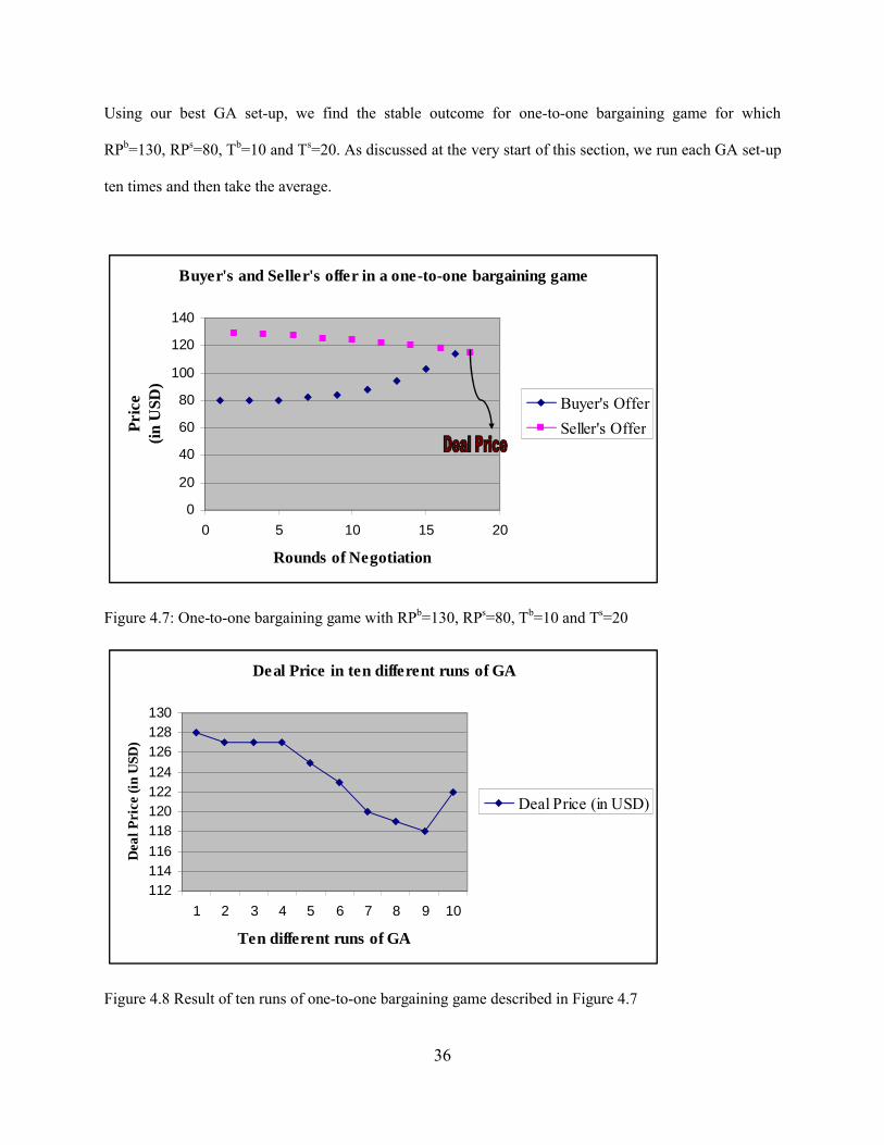
Using our best GA set-up, we find the stable outcome for one-to-one bargaining game for which

RPb=130, RPs=80, Tb=10 and Ts=20. As discussed at the very start of this section, we run each GA set-up

ten times and then take the average.

Buyer's and Seller's offer in a one-to-one bargaining game

0

20

40

60

80

100

120

140

0 5 10 15 20

Rounds of Negotiation

Pri

ce(i

n U

SD)

Buyer's Offer

Seller's Offer

Figure 4.7: One-to-one bargaining game with RPb=130, RPs=80, Tb=10 and Ts=20

Deal Price in ten different runs of GA

112114116

118120122124

126128130

1 2 3 4 5 6 7 8 9 10

Ten different runs of GA

Dea

l Pri

ce (i

n U

SD)

Deal Price (in USD)

Figure 4.8 Result of ten runs of one-to-one bargaining game described in Figure 4.7

37

Figure 4.7 shows one such run displaying the successive offers made by the buyer and the seller in

different rounds of negotiation. Figure 4.8 shows the deal price (stable outcome) in all ten experiments. It

can be noticed that the GA does not give the same results and sometimes can give the sub-optimal results.

This is why we run the same GA program ten times and then average the results. The average deal after

ten experiments was found to be 123.

4.2 EXPERIMENT 2

In this experiment, we compare the performance of the genetic algorithm with random search. We find

the stable outcome using these two methods where the (RPs, RPb) couplet is (80,130), Tb =10 and Ts=50

(if the seller’s deadline is greater than the buyer’s deadline, otherwise Tb =50 and Ts=10).

Buyer's and Seller's offers in a bargaining game using Random Search when buyer's deadline < seller's deadline

0

20

40

60

80

100

120

140

0 5 10 15 20

Rounds of negotiation

Dea

l Pri

ce (

in U

SD)

Buyer's Offer

Seller's Offer

Figure 4.9 One-to-one bargaining game with RPb=130, RPs=80, Tb=10 and Ts=50 using random search

It is clear from Figures 4.9 and 4.10 that the random search does not converge but the genetic algorithm

converges. In random search, when the seller’s deadline is very high as compared to the buyer’s deadline,

the offers proposed by the seller remains almost constant and the buyer’s offers keep on fluctuating.

However, using the genetic algorithm, the buyer’s offers converge fast because of a low deadline but the

38

Buyer's and Seller's offers in a bargaining game using Genetic Algorithm when buyer's deadline < seller's deadline

0

20

40

60

80

100

120

140

0 5 10 15 20

Rounds of negotiation

Dea

l Pri

ce (

in U

SD)

Buyer's Offer

Seller's Offer

Figure 4.10 One-to-one bargaining game with RPb=130, RPs=80, Tb=10 and Ts=50 using genetic

algorithm

Buyer's and Seller's offers in a bargaining game using Random Search when buyer's deadline > seller's deadline

0

20

40

60

80

100

120

140

0 5 10 15 20

Rounds of negotiation

Dea

l Pri

ce (

in U

SD)

Buyer's Offer

Seller's Offer

Figure 4.11 One-to-one bargaining game with RPb=130, RPs=80, Tb=50 and Ts=10 using random search

seller’s offers converge very slowly because of a higher deadline. The stable outcome is fairly close to

RPb as expected. Similarly, in Figures 4.11 and 4.12, again we see that the random search fails to

converge. The buyer’s deadline is greater than the seller’s deadline and the offers proposed by the buyer

39

remains almost constant. The offers made by the seller keep on fluctuating. Again, using the genetic

algorithm, we see in Figure 4.12 that the stable outcome is fairly close to RPs, because the buyer’s

deadline is greater than the seller’s deadline. Hence we conclude that the random search fails miserably

when compared to the genetic algorithm.

Buyer's and Seller's offers in a bargaining game using Genetic Algorithm when buyer's deadline > seller's deadline

0

20

40

60

80

100

120

140

0 5 10 15 20

Rounds of negotiation

Dea

l Pri

ce (

in U

SD)

Buyer's Offer

Seller's Offer

Figure 4.12 One-to-one bargaining game with RPb=130, RPs=80, Tb=50 and Ts=10 using genetic algorithm

4.3 EXPERIMENT 3

In Section 3.2, we described bargaining as a search problem where the genetic algorithm (GA) is used to

find the stable outcome. In the game theoretic technique, we have the concept of equilibrium but in a

genetic algorithm approach, the equilibrium is the stable outcome. Since a GA is not guaranteed to

converge and give the same result each time it runs, we run the same GA ten times and then take the

average. We notice that the variation in the stable outcome increases with an increasing size of the zone

of agreement (Z). We calculate the variation in deal price as:

Variation in deal price (in %) = (Max. –Min)*100/Min

where Max = maximum value of the deal price obtained in ten runs of the GA

40

Min= minimum value of the deal price obtained in ten runs of the GA

In Figure 4.13 we show the variation in the deal price in five different cases. The (RPs, RPb) in these cases

are (80,100), (80,200), (80,300) (80,400) and (80,500). Hence, the sizes of Z in these cases are 20, 120,

220, 320 and 420. We see that the variation in deal price increases with the size of Z. This is because the

search space increases accordingly with the increasing size of Z and the GA does not converge at the

same point, leading to variation in results. This also means that a buyer who has a very high reserve price

pays more than the one with a lower reserve price.

Effect of increasing size of Zone of agreement (Z) on variation in Deal Price

0

100

200

300

400

500

0 2 4 6 8

Variation in Deal Price(in %)

Size

of

Zon

e of

Agr

eem

ent

Variation in DealPrice

Figure 4.13: Effect of increasing the size of the zone of agreement (Z) on variation in Deal Price

4.4 EXPERIMENT 4

In order to measure the effectiveness of Cyber Haggler, we compare the performance of Cyber Haggler

with human-to-human bargaining in five different games. The (RPs,RPb) couplet were (20, 40), (40,80),

(60,120), (80,160) and (100,200). We analyze the results for two different situations. Firstly, when the

seller’s deadline is greater than the buyer’s deadline and secondly, when the seller’s deadline is less than

the buyer’s deadline. In human-to-human bargaining both the buyers and the sellers know each others

reserved prices but do not know each other’s deadlines. All the participants were students of The

41

University of Georgia. A third person acts as a mediator to start and end the bargaining in accordance

with the bargaining protocol. Human-to-human bargaining is exactly the same as our proposed model

except for the fact that it does not involve any computer program and uses a mediator to start and end the

bargaining process.

Comparison of Deal Price between Cyber Haggler and Human-to-Human bargaining when seller's deadline is

greater than buyer's deadline

0

50

100

150

200

250

0 2 4 6

Five one-to-one bargaining games

Dea

l Pri

ce(i

n U

SD) Cyber Haggler

Human-to-HumanBargaining

Figure 4.14: Comparison of Cyber Haggler with human-to-human bargaining in five different games with seller’s deadline being greater than buyer’s deadline

In Figure 4.14 we see that the stable outcome of Cyber Haggler benefits the seller more when compared

to human-to-human bargaining. This is consistent with the game theoretic equilibrium when the seller’s

deadline is greater than the buyer’s deadline. The same can be inferred from Figure 4.15. One limitation

of this experiment is that the results of human-to-human bargaining depends on a number of factors such

as whether the person is really good at bargaining or not, the utility function of bargainer, etc. In sum, the

results of human-to-human bargaining can be different in different cases and it is very likely that they can

outperform Cyber Haggler. However, our aim in this thesis is to develop intelligent and adaptive

bargaining agents and we do not claim that Cyber Haggler will outperform every human bargainer.

42

Comparison of Deal Price between Cyber Haggler and Human-to-Human bargaining when seller's deadline is lesser

than buyer's deadline

020406080

100120140160

0 2 4 6

Five one-to-one bargaining games

Dea

l P

rice

(in

US

D) Cyber Haggler

Human-to-HumanBargaining

Figure 4.15: Comparison of Cyber Haggler with human-to-human bargaining in five different games with buyer’s deadline being greater than seller’s deadline

4.5 EXPERIMENT 5

In this experiment, we test our model in one-to-many bargaining game. The assumptions and the

bargaining protocol for this model are same as discussed in Chapter 3. A buyer with RPb=130 is

bargaining simultaneously with three sellers each having different reservation price. RPs1=70, RPs2=80

and RPs3=90. The deadline of the buyer is Tb=10 and the deadline of the sellers is Ts1 = 40 (seller 1), Ts2 =

30 (seller 2) and Ts3 = 20 (seller 3). We see that the seller having the lowest reservation price has the

highest deadline and vice versa. The reason for this choice was to examine the results in such a situation

because a seller with the lowest reservation price as well as the lowest deadline will eventually win the

deal over the other sellers. Figure 4.12 shows the offers made by different sellers and buyers in different

rounds of negotiation. We see that the offers made by seller 1 are always lower than those of the other

sellers and eventually seller 1 wins the deal in the final round of negotiation. Since seller 1 has the lowest

reservation price, even though it has a longer deadline, it beats the other sellers, albeit marginally. Hence,

it can be interpreted that the algorithm will always favor a seller with a lower reservation price and

43

preferably a lower deadline. Even though the deadline is not the lowest, a very low reservation price can

result in a successful deal as is evident from our experiment.

One-to-many bargaining game

0

20

40

60

80

100

120

140

0 5 10 15 20

Rounds of negotiation

Pri

ce(i

n U

SD) Buyer's Offer

Seller 1 with RP=70

Seller 2 with RP=80

Seller 3 with RP=90

Figure 4.16: One-to-many bargaining game with one buyer and three sellers each having different deadline and different reservation price

44

CHAPTER 5

CONCLUSION

5.1 INTRODUCTION

In this Chapter we provide summary and potential directions for future research.

5.2 SUMMARY

We have developed a web-based bargaining website Cyber Haggler (http://www.cyberhaggler.com).

Game theory has excessive research on the bargaining models under the assumption of perfect rationality.

However, we are interested in one-to-one and one-to-many sequential bargaining models where the

players (buyers and sellers) exhibit bounded rationality. Our aim in this thesis is to develop intelligent

buyer and seller agents that learn from trial-and-error to reach a deal. They should be able to simulate

human-type reasoning. For example: consider the situation of a haggler who goes to a flea market and

starts bargaining for a product such as a used guitar. As a buyer, he sets a reserved price for the guitar and

plans to make all offers up to and including his reserved price. Similarly, the guitar seller also sets a

reservation price in his mind and plans not to accept any offer less than his reservation price. The buyer

starts from a very small offer and increases it. Similarly the seller asks for a very high price and decreases

it. The moment an offer is mutually acceptable a deal is made. We capture the same process and

implement it as a genetic algorithm. We could have encoded game theoretic equilibrium rules into a well-

structured knowledge-based system, but this approach cannot include automated learning. Also, this

approach would have been very inflexible. Thus, we pose the bargaining problem as a search and

optimization problem and use a genetic algorithm to find an equilibrium point in the search space. Also,

while game theory assumes that the players have perfect rationality and complete knowledge, we make

our model more realistic by assuming that the players have bounded rationality and partial knowledge. In

our genetic algorithm model, we have two subpopulations, one for the buyer and the other for the seller.

45

We evolve these populations and the stable outcome becomes the deal price. While the game theoretic

approach has an equilibrium point, the genetic algorithm approach has a stable outcome where the buyer

and the seller populations offer the same price to each other. We started with a discussion on bargaining

theory in Chapter 1. In Chapter 2, we discussed the most relevant work related to our thesis. Most

importantly is Kasbah. In Chapter 3, we gave the details of our negotiation model. Also, we discussed the

differences between Cyber Haggler and Kasbah, and Cyber Haggler and EBay. In Chapter 4, we

conducted various experiments to test our model. Experiment 1 aimed at finding an optimal parameter set

up for the genetic algorithm, Experiment 2 compared the performance of the genetic algorithm with

random search, Experiment 3 showed the variation of the deal price with the increasing size of the zone of

agreement, Experiment 4 compared Cyber Haggler with human-to-human bargaining; and Experiment 5

discussed the one-to-many bargaining model.

5.3 FUTURE WORK

Though we have developed a fairly significant and very realistic model of bargaining, there are many

more aspects to be developed in a versatile real world bargaining model. We can extend our present work

in the future. Future work may include the following:

The present work deals with price as the only issue. The model could be extended to a multi-issue

bargaining model including price, quality, quantity, delivery time, payment method, and more.

In the present model, the buyer can search results in real time and haggle to get a deal

immediately. The seller could utilize such capabilities. In this way, a seller can find all the

interested buyers in real time and start the bargaining process to obtain a deal immediately.

Currently, a default value is used for the buyer’s deadline. A better idea would be to estimate the

buyer’s deadline based on attributes such as the utility value of the product, number of buyers

contending for the product at any time, the buyer’s per month transactions with Cyber Haggler,

and so on.

46

Bargaining is a complex problem for which we have proposed a web-based and user-friendly

model and an implementation. Cyber Haggler covers all the features of a good bargaining model.

It may prove to be an important work in the development of web-based bargaining models.

47

REFERENCES

[1] Bazerman, M., T. Magliozzi, and M. Neale. “Integrative bargaining in a competitive market.”Organization Behavior and Human Decision Processes, 35:294–313, 1985.

[2] Chavez, Anthony, and Maes, “Kasbah: An agent marketplace for buying and selling Goods,” MIT Media Lab, http:// agents.www.media.mit.edu:80/groups/ agents/ Publications/ kasbah_paam96.ps, July 1996.

[3] Faratin, P., C. Sierra, and N. R. Jennings. “Negotiation decision functions for autonomous agents.”International Journal of Robotics and Autonomous Systems, 24(3-4):159–182, 1998.

[4] Fatima, S. S., M. Wooldridge, and N. R. Jennings. “A Comparative Study of Game Theoretic and Evolutionary Models of Bargaining for Software Agents,” Proceedings of the Artificial Intelligence Review, 23:185-203

[5] Fatima, S. S., M. Wooldridge, and N. R. Jennings. “Comparing Equilibria for Game-Theoretic and Evolutionary Bargaining Models,” Proceedings of the Fifth International Workshop on Agent-Mediated Electronic Commerce (AMEC-2003), Melbourne, Australia, July 2003.

[6] Holland, J.H. (1975) Adaptation in Natural and Artificial Systems, Ann Arbor, MI: University of Michigan Press, 1975.

[7] Liang, Ting-Peng, Her-Sen Doong, “Effect of Bargaining in Electronic Commerce,” Workshop on Advanced Issues of E-Commerce and Web/based Information Systems (WECWIS-1999): 174-181

[8] Nash, J.F., “The bargaining problem,”Econometrica 18 (1950) 155–162.

[9] Raiffa, H., The Art and Science of Negotiation, Belknap/Harvard U. Press, 1982.

[10] Raymond Y. K. Lau: “Towards Genetically Optimised Multi-Agent Multi-Issue Negotiations.”Hawaii International Conference on System Sciences (HICSS) 2005

[11] Roth, A. E., “Bargaining experiments,” In J. Kagel and A. E. Roth, editors, Handbook of Experimental Economics. Princeton, NJ: Princeton University Press, 1995.

[12] Rubinstein, A., “A bargaining model with incomplete information about time preferences,” Econometrica, 53:1151–1172, January 1985.

[13] Rubinstein, A., Perfect equilibrium in a bargaining model, Econometrica, 50(1):97–109, January 1982.

[14] Sandholm, T. and N. Vulkan. “Bargaining with deadlines.” Proceedings of the Association for the Advancement of Artificial Intelligence (AAAI-99), 44–51, Orlando, FL, 1999.

48

[15] Sheng, Y. P., Z Chen, “Online Bargaining as a Form of Dynamic Pricing and the Sellers' Advantage from Information Asymmetry” Proceedings of the Americas' Conference on Information Systems (AMCIS-2005), Omhaha,Nebraska, 2005.

[16] Zeng, D, and K Sycara, “Bayesian learning in negotiation,” Working Notes of the AAAI 1996 Stanford Spring Symposium Series on Adaptation, Coevolution, and Learning in Multiagent Systems, Stanford University, Palo Alto, CA 1996, also http://www.cs.cmu.edu/~zeng.