danks ms thesis 2007

SPATIAL, TEMPORAL, AND LANDSCAPE CHARACTERISTICS OF MOOSE-VEHICLE COLLISIONS

IN MAINE

by

Zachary David Danks

A thesis submitted in partial fulfillment

of the requirements for the Master of Science Degree

State University of New York

College of Environmental Science and Forestry Syracuse, New York

July 2007 Approved: Department of Environmental and Forest Biology ______________________________ ___________________________ Dr. William F. Porter, Major Professor Dr. George W. Curry, Chair, Examining Committee ______________________________ ___________________________ Dr. Donald J. Leopold, Department Dr. Dudley J. Raynal, Dean, Chair Instruction and Graduate Studies © Copyright Zachary David Danks All rights reserved

ii

ACKNOWLEDGEMENTS

Funding for this research was provided by the American Wildlife

Conservation Foundation, the Research Foundation of the State University of New

York, and the Department of Environmental and Forest Biology at SUNY-ESF. I

received additional support from Elk Lake Lodge and from SUNY-ESF as a Webb

Apprentice and staff member at the Adirondack Ecological Center. Data were

generously provided by John Perry and Greg Costello of the Maine Department of

Transportation and by Karen Morris of the Maine Department of Inland Fisheries and

Wildlife. The Quantitative Studies Lab at SUNY-ESF and the Adirondack Ecological

Center at the Huntington Wildlife Forest provided computer-related resources.

Completion of this thesis would not have been possible without the assistance

of many important people. First, I thank my major professor, Dr. William F. Porter,

for recognizing the potential for this research and for a quality work environment full

of helpful people and resources. His guidance and confidence in me were critical and

permitted me to develop a project pursuant to my interests in wildlife biology. I thank

also my committee members, Stacy McNulty and Drs. Jacqueline Frair, H. Brian

Underwood, James Gibbs, and George Curry; their critical review and helpful

suggestions greatly strengthened my thesis. Drs. Steve Stehman, Lianjun Zhang, and

Paul Bern provided additional statistical advice.

I am particularly grateful for the support of all QSL members that I have been

associated with. Ben Zuckerberg and Jeff Organ never failed to discuss GIS and stats

issues. I enjoyed working for and alongside Amy Dechen on her Chronic Wasting

iii

Disease research. Carolyn Spilman, Annie Woods, Frank DeSantis, Sarah Nystrom,

and Elizabeth Dowling were fun and indispensable friends during my time at ESF.

All provided many critical reviews of my work and endless encouragement.

I learned much from Ray Masters, Charlotte Demers, Stacy McNulty, Paul

Hai, Steve Signell, Marianne Patinelli-Dubay, Mike Gooden, and Bruce Breitmeyer at

the Adirondack Ecological Center. My time at the Huntington Wildlife Forest was

greatly enjoyed, due in no small part to their tutelage and friendship.

I thank John and Margot Ernst and Mike and Cammy Sheridan, who let me

live and work at Elk Lake Lodge – a magnificent spot in the Adirondacks. It was a

joy to know the many wonderful staff members, all of whom I consider family.

I acknowledge my early mentors in wildlife science from Kentucky – Drs. Jeff

Larkin, Karen Alexy, John Cox, and David Maehr, and Mike Orlando – who let me

work on some very exciting fieldwork and introduced me to the graduate experience.

My biggest thanks goes to my family, who remained steadfast in their support

of me through the hardest and best of times. In particular, I thank: my father David,

for teaching me to respect and appreciate our land and wildlife resources; my mother

Jeanie, for teaching me compassion and how to communicate genuinely with people;

and my sister Jennie, for teaching me that endless devotion to a big brother is among

life’s most precious blessings. Also, I am proud to have had the tireless support of

Elizabeth Dowling – my fiancée – whom I am lucky to have met while at ESF; I am

excited to share my life with such a wonderful, bright woman. The love and patience

of my family and my Maker could not have been appreciated more.

iv

TABLE OF CONTENTS

ACKNOWLEDGEMENTS .......................................................................................... ii

TABLE OF CONTENTS..............................................................................................iv

LIST OF TABLES ........................................................................................................vi

LIST OF FIGURES .................................................................................................... vii

LIST OF APPENDICES ............................................................................................ viii

ABSTRACT..................................................................................................................ix

INTRODUCTION ........................................................................................................ 1

STUDY AREA ............................................................................................................. 3

METHODS ................................................................................................................... 6

Data Collection…………………………………………………………………….. 6

Moose-vehicle collisions………………………………………………………... 6

Roads……………………………………………………………………………. 7

Land cover and topography……………………………………………………... 8

Moose harvest…………………………………………………………………… 8

Temporal Patterns of Moose-Vehicle Collisions…………………………………...9

Spatial Patterns of Moose-Vehicle Collisions……………………………………... 9

K-function analysis……………………………………………………………… 9

Kernel density analysis………………………………………………………… 11

Landscape Characteristics of Moose-Vehicle Collisions………………………… 12

GIS analysis……………………………………………………………………. 12

Statistical analysis………………………………………………………………14

v

RESULTS ................................................................................................................... 16

Temporal Patterns of Moose-Vehicle Collisions………………………………….16

Spatial Patterns of Moose-Vehicle Collisions……………………………………. 17

K-function analysis…………………………………………………………….. 17

Kernel density analysis………………………………………………………… 17


DISCUSSION............................................................................................................. 22

Temporal Patterns of Moose-Vehicle Collisions………………………………… 22

Spatial Patterns of Moose-Vehicle Collisions……………………………………. 26


MANAGEMENT IMPLICATIONS .......................................................................... 36

LITERATURE CITED ............................................................................................... 38

APPENDICES ............................................................................................................ 81

VITA ........................................................................................................................... 84

vi

LIST OF TABLES

1. Land cover reclassification of Maine GAP Analysis land cover imagery of Maine, USA, 1991-1993..............................................................................51

2. Landscape covariates measured for locations of moose-vehicle collisions

and random points on roads in western Maine, USA, 1992-2005. ..................52 3. Candidate logistic regression models used to predict moose-vehicle

collisions in western Maine, USA, 1992-2005.. ..............................................54 4. Descriptive statistics of landscape covariates measured for locations of

moose-vehicle collisions and random points on roads in western Maine, USA, 1992-2005. .............................................................................................56

5. Descriptive statistics of landscape covariates measured for locations of

moose-vehicle collisions and random points on roads statewide in Maine, USA, 1992-2005. .............................................................................................57

6. Model-fitting results for logistic regression models used to predict

moose-vehicle collisions in western Maine, USA, 1992-2005........................58 7. Coefficient estimates from the final (reduced) logistic regression model

used to predict moose-vehicle collisions in western Maine, USA, 1992-2005..................................................................................................................59

8. Validation results of logistic regression modeling used to predict moose-

vehicle collisions in western Maine and statewide, Maine, USA, 1992-2005..................................................................................................................60

vii

LIST OF FIGURES

1. Locations of moose-vehicle collisions in western Maine, USA, 1992-2005..................................................................................................................61

2. Density per km2 of roads, moose-vehicle collisions, and hunter harvest of

moose in townships of Maine, USA, 1992-2005.. ...........................................63 3. Temporal distribution of moose-vehicle collisions in the western Maine

study area and statewide, Maine, USA, 1992-2005.........................................65 4. Plotted values of the L-statistic for network K- function analysis of

moose-vehicle collisions in western Maine, USA, 1992-2005........................67 5. Fixed kernel density estimations of moose-vehicle collisions in western

Maine, USA, 1992-2005. .................................................................................69 6. Clusters of moose-vehicle collisions and random points identified

through kernel density analysis in western Maine, USA, 1992-2005..............71 7. Predicted probability of moose-vehicle collisions against landscape

predictor covariates, western Maine, USA, 1992-2005 ...................................73 8. Predicted probability of moose-vehicle collisions against traffic volume

shown by level of speed limit, western Maine, USA, 1992-2005.. .................75 9. Mean values of land cover composition covariates calculated within

buffers surrounding moose-vehicle collisions and random points in western Maine, USA, 1992-2005.....................................................................77

10. Mean or proportional values of land cover configuration covariates

calculated within buffers surrounding moose-vehicle collisions and random points in western Maine, USA, 1992-2005. .......................................79

viii

LIST OF APPENDICES

1. APPENDIX A. Calculation of human population density in Maine using 2000 Census Bureau data. ................................................................................81

2. APPENDIX B. Description of the K- function and network K- function. .........82

ix

ABSTRACT

Danks, Zachary D. Spatial, temporal, and landscape characteristics of moose-vehicle collisions in Maine. Word processed and bound thesis, 84 pages, 8 tables, 10 figures, 2 appendices, 2007. I analyzed moose (Alces alces)-vehicle collisions (MVCs) in Maine from 1992-2005 using spatial statistics and Geographic Information Systems (GIS). My objectives were to describe temporal and spatial distributions of MVCs and to develop predictive models based on landscape characteristics. MVCs were most frequent from June-October and clustered spatially at local and regional scales. Logistic regression modeling showed that the predicted probability of MVC increased by 57% for each 500-vehicle/day increase in traffic volume, by 35% for each 8-km/hour increase in speed limit, and by 36% for each 5% increase in cutover forest cover. Land cover covariates were most explanatory at spatial extents (2.5-5 km) that approximated the spatial requirements of moose. Where the reduction of timber harvesting, conifer cover, and wetlands over large areas is not feasible, lowering driving speeds during high-risk times of day and year and in high risk areas may be most effective for reducing MVCs. Key words: Alces alces, collision, cutover, Geographic Information System, GIS, landscape characteristics, Maine, moose, motor vehicles, traffic Author’s name in full: Zachary David Danks Candidate for degree of: Master of Science Date: July 2007 Major Professor: William F. Porter Department: Environmental and Forest Biology State University of New York College of Environmental Science and Forestry, Syracuse, New York.

Signature of Major Professor: _____________________________________

1

INTRODUCTION

Transportation and wildlife agencies across North America face the challenge

of reducing motor vehicle collisions with large mammals. Although most large

mammal-vehicle collisions involve deer (Odocoileus spp.), collisions involving

moose (Alces alces) pose greater safety risks to motorists due to the large body size

(360-600 kg) and high center of gravity of moose (1.85-1.95 m; Bubenik 1998).

Moose-vehicle collisions (MVCs) can lead to the injury or death of vehicle occupants

and moose, vehicle damage, losses of recreational opportunities such as moose

hunting and viewing, increased insurance premiums, and increased public

dissatisfaction with moose presence along roads (Child and Stuart 1987, Child 1998,

Schwartz and Bartley 1991).

Approximately 2,500-3,000 MVCs occur annually in the United States and

Canada, but this estimate is conservative because many MVCs go unreported (Child

and Stuart 1987, Child 1998). In several northern states and Canadian provinces,

hundreds of MVCs are reported each year, which in some regions constitutes a

significant proportion of the annual allowable hunter harvest of moose (Child 1998).

In regions where mammalian predators of moose are absent, such as New England,

MVCs may constitute the primary source of non-hunting mortality of moose (Peek

and Morris 1998). Projected moose population increases in urbanized jurisdictions

like Massachusetts and New York may lead to more frequent MVCs (Hicks and

McGowan 1992, Vecellio et al. 1993).

2

Maine currently supports the largest moose population in the lower 48 states

(Peek and Morris 1998). Each year 600-700 MVCs occur in Maine, imposing an

estimated annual economic impact of $17.5 million (Farrell et al. 1996, MIFW 2006).

From 1996-1998 there were =14,900 motor vehicle collisions in Maine involving

moose, white-tailed deer (O. virginianus), or black bears (Ursus americanus), which

resulted in 10 human fatalities and combined economic losses of =$101 million

(MIWG 2001).

Collisions involving moose may result from several factors related to

population levels, roads, and habitat. Seasonal behaviors associated with foraging,

parturition, dispersal, and breeding probably influence moose presence along roads

(MIWG 2001). When near roads, individual moose face risks from traffic and

inattentive motorists, which can greatly influence the amount and location of MVCs

(Belant 1995, Joyce and Mahoney 2001, Seiler 2005, Hurley 2007). The amount and

configuration of adjacent habitat may also be important predictors of MVCs (MIWG

2001; Seiler 2004, 2005). Certain habitat features can attract moose to roadsides to

feed (Child 1998), and topographic features or road structures can funnel moose

movements across roads (Clevenger et al. 2001). Weather and time of day coinciding

with peaks in human and moose activity may be confounding variables that promote

the occurrence of MVCs (Joyce and Mahoney 2001, Dussault et al. 2006b).

Interactions of these factors may produce patterns of collisions that are aggregated

temporally and spatially, such that certain roads contain disproportionately higher

numbers of collisions (Joyce and Mahoney 2001, Malo et al. 2004). Additionally,

3

spatial distributions of wildlife-vehicle collisions likely vary with spatial scale, which

affects how and where mitigation projects are employed (Clevenger et al. 2003, Malo

et al. 2004).

Improved understanding of the temporal and spatial distributions of MVCs

and landscape characteristics associated with their occurrence could improve

managers’ ability to predict high-collision locations and prioritize mitigation efforts. I

sought to address this management need within the state of Maine where MVCs are

an ecological, economic, and political problem. Based on prior studies of large-

mammal vehicle collisions and moose ecology, I hypothesized that MVCs in Maine

would (1) be distributed non-randomly in time or space; (2) be related to moose

abundance, traffic, and habitat; and (3) be a product of landscape-scale habitat

influences reflective of the life history and spatial requirements of moose. To address

these hypotheses, my objectives for this study were to (1) describe temporal and

spatial distribution patterns of MVCs, (2) determine relationships between landscape

characteristics and the risk of MVCs, and (3) identify geographic extents at which

habitat management might effectively reduce MVCs.

STUDY AREA

I studied the effects of landscape factors on MVCs at both a regional and

statewide level in the state of Maine. Maine is located between 42° 58’40” and 47°

27’33” North latitude and 66° 56’48” and 71° 06’41” West longitude. The physical

geography of Maine varies by latitude, longitude, and altitude, and was shaped by

glaciers as recently as 11,000 YBP. Across the state, terrain varies from low (<200 m

4

above seal level), gently sloping hills in coastal regions, to hilly uplands (200-450 m)

in interior and northeastern regions, to mountains (300-1,606 m) in western and

northwestern regions (McMahon 1990, Boone 1997).

Maine is characterized by extensive forest on uplands and lowlands, rivers and

small streams, brackish and freshwater wetlands, and inland lakes (Krohn et al. 1998).

Vegetation patterns in Maine vary regionally in accordance with climate, which is

influenced by latitude, elevation, distance from the coast, and by the southwest-

northeast orientation of the mountains and coast (Fobes 1946, McMahon 1990).

Species richness of woody plants increases 2-fold from north-western to south-eastern

Maine in response to climatic gradients (McMahon 1990). Three major forest

associations are present in Maine: spruce (Picea spp.) - fir (Abies balsamea) -

northern hardwoods (beech [Fagus grandifolia], yellow birch [Betula alleghaniensis],

sugar maple [Acer saccharum]) in the northern and mid- and east-coastal regions;

northern hardwoods - hemlock (Tsuga canadensis) - white pine (Pinus strobus) in

portions of the central and eastern regions; and transition hardwoods (oak [Quercus

spp.], hickory [Carya spp.], ash [Fraxinus spp.]) - white pine - hemlock in

southwestern and south-central regions (Westveld et al. 1956). Most of Maine’s

northern forests are owned by private timber companies and contain varying

proportions of clear-cut, partially cut, and mature forest age classes (Griffith and

Alerich 1996, Luppold 2004).

McMahon (1990) delineated 15 biophysical regions in Maine based on

relationships between the distributions of woody plant species and several

5

environmental variables, such as climate, topography, geology, and soils. The

biophysical classification incorporates both biological and environmental

characteristics and provides a useful framework for conducting ecological analyses at

a regional scale. In addition to a statewide scale, I chose the Western Mountains

biophysical region (hereafter referred to as western Maine) for a regional study area

for my analysis of MVCs (Figure 1; MEGIS 1991). Western Maine (latitude 45° 25'

north, longitude 70° 35' west) is a 10,271-km2 area bounded by mountains along the

Maine-Quebec border to the North, the Mahoosuc Range to the Southwest, and the

330-m contour and several lower elevation valleys west of Moosehead Lake to the

East (McMahon 1990). The region has a low human population density (4.1

persons/km2) compared to the statewide average for Maine (29.9 persons/km2;

Appendix I). The climate is characterized by cool summers (mean maximum July

temperature = 23.9 C), cold winters (mean minimum January temperature = -18.1 C)

with high annual snowfall (mean = 280 cm), and low annual precipitation (mean =

98.4 cm). Elevation averages 330-660 m, with several peaks above 1,000 m

(McMahon 1990). Terrain is mountainous with steep stream drainages and several

large lakes. Vegetation is predominately forested; mid-elevation uplands and well

drained lowlands are composed of northern hardwood forests, while ridges are

typically stands of balsam fir and red spruce (Picea rubens). Paper birch (B.

papyrifera), aspen (Populus spp.), and red maple (A. rubrum) are common on

mountain slopes and poorly drained areas. Lowland conifers include black spruce

6

(Picea mariana), northern white cedar (Thuja occidentalis), and tamarack (Larix

laricina).

My analysis is based on the system of local, state, and national highways in

Maine as represented by a roads data set maintained by the Maine Department of

Transportation (MDOT; G. Costello, MDOT, unpublished data). The state highway

system serves arterial and through traffic and is maintained primarily by MDOT

(MDOT 2006c). Roads included in the analysis are classified according to the Federal

Functional Classification of Highways, which includes 4 general categories of paved

roads: principal arterial, minor arterial, collector, and local (MDOT 2006b). In the

MDOT road system, there are approximately 35,783 km (0.4 km/km2) of paved

highway statewide and approximately 2,492 km (0.2 km/km2) in western Maine.

METHODS

Data Collection

Moose-vehicle collisions.—I obtained MVC data from MDOT (MDOT

Accident Records Section, unpublished data). These data consisted of MVCs (n =

8,156) recorded throughout the state of Maine from 1992-2005 (Figure 1). The data

represented MVCs that were reported by state, county, or local police when either a

human injury or =$1,000 ($500 prior to 1999) in property damage resulted from the

collision (MDOT 2006a). Police recorded the location of each MVC with software on

a laptop computer that referenced the MVC location to the state road network, but not

necessarily by mile-marker (Hubbard et al. 2000). The MDOT Accident Records

Section reviewed the police records to verify spatia l accuracy of reported location

7

information (estimated as ±0.16 km; G. Costello, MDOT, personal communication)

and compiled the data into a shapefile for use in a Geographic Information System

(GIS).

Given the monetary threshold for collision reporting, these data represent a

conservative sample of the actual number of MVCs that occur on Maine roads.

Numbers of MVCs may be underrepresented on local roads not maintained by

MDOT, and MVCs that do not meet the property damage threshold or do not cause a

human injury may not be reported (G. Costello, MDOT, personal communication).

Usually MVCs are fatal for the moose involved (Farrell et al. 1996, Seiler 2004), but

because some MVCs do not result in the death of the animal, these data do not fully

represent mortality of moose via motor vehicle collisions. Moose-vehicle collisions

have been under-reported in Sweden and other North American jurisdictions

(Almkvist et al. 1980 [cited in Seiler 2004], Child and Stuart 1987). Despite the

limitations of the collision-reporting procedure, I assumed the data were

representative of MVCs that occurred in Maine from 1992-2005.

Roads.—I obtained roads, speed limit, and traffic volume data from MDOT.

The roads data consisted of a statewide network of paved road segments that had been

classified by MDOT according to the Federal Functional Classification of Highways

(MDOT 2006b). Speed limit (km/hour) and traffic volume (annual average daily

traffic) data had been recorded for each road link in the statewide road network and

were provided by MDOT as shapefiles.

8

Land cover and topography.—I derived habitat variables from a land cover

map of Maine produced by the U.S. Geological Survey Biological Resources

Division GAP Analysis Program (ME-GAP; Krohn et al. 1998). The ME-GAP land

cover map consists of classified LANDSAT Thematic Mapper (TM) imagery

acquired in 1991 and 1993, with 30 X 30-m resolution and 37 land cover classes

depicting forested lands (9 classes), wetlands (18 classes), agricultural lands (4

classes), developed lands (4 classes) and other lands (2 classes). Overall classification

accuracy of the ME-GAP land cover map was 88.1% (Krohn et al. 1998). I

reclassified land cover classes using the Spatial Analyst extension in ArcMap 9.1

(ESRI 2004), which reduced the number of cover classes from 37 to 11 (Table 1). I

reclassified ME-GAP land cover classes as cover types used in assessments of

landscape- level habitat suitability for moose (Allen et al. 1987, Koitsch 2003). For

streams and areas of human development, I used shapefiles depicting features shown

on USGS 1:24,000 quadrangles (MEGIS 1992a, b).

For topographic variables, I used a 30 X 30-m resolution digital elevation

model (DEM) of Maine from the United States Geological Survey (USGS; USGS

2006). I derived slope and aspect layers from the DEM using Spatial Analyst.

Moose harvest.—In addition to records of MVCs, I obtained moose harvest

data from the Maine Department of Inland Fisheries and Wildlife (MIFW; K. Morris,

MIFW, unpublished data). Harvest data consisted of the number of hunter-harvested

moose reported annually by township from 1992-2005. During this period, moose

hunting was allowed in 691 of 917 townships (75%) in Maine, all of which were

9

located in northern portions of the state (Figure 2). Moose harvest statistics were

biased towards areas that received the highest hunting pressure, which were cutover

areas on privately-owned timber company lands having a network of logging roads

that permit access for hunters (K. Morris, MIFW, personal communication). Seiler

(2005) noted limitations of using harvest statistics to index moose abundance, but

nonetheless used them in a study of MVCs in Sweden. In the absence of better

information on the spatial distribution of moose in Maine, I indexed the moose

population by averaging the annual moose harvest/township across years and

standardizing by township area. The resulting variable represented the annual average

number of hunter-harvested moose/10km2 by township.

Temporal Patterns of Moose-Vehicle Collisions

To describe temporal patterns of MVCs in western Maine and statewide, I

compared the frequency of MVCs across months, times of day, and years using chi-

square (?2) analysis. I calculated the ratio of annual MVC frequency to annual moose

harvest as a simple index of the proportional relationship between MVCs and moose

abundance (Seiler 2004). I used the Spearman rank correlation coefficient (PROC

CORR; SAS Institute 2006) to assess the correlation (r) between annual MVC

frequency and year, annual harvest and year, annual MVC frequency and annual

harvest, and the MVC/harvest ratio and year.

Spatial Patterns of Moose-Vehicle Collisions

K-function analysis.—To describe spatial patterns of MVCs, I used K-

function analysis to quantify the degree of clustering of MVC point locations across a

10

range of spatial scales. The K-function (Appendix B; Bailey and Gatrell 1995) uses

the Euclidean distance between all points of interest within a homogenous spatial

region to calculate the number of neighboring points within a specified radial distance

increment t of each point in the data set. The distance increments t can be thought of

as the radii of concentric circles placed over each point i, such that the number of

points j occurring within t is counted (Bailey and Gatrell 1995). By specifying

multiple t, the user can determine, across several scales, whether the observed spatial

distribution of points varies from a random Poisson distribution (i.e., a regular or

clustered distribution).

To account for the distribution of MVC points along the linear road network

rather than a homogeneous 2-dimensional area (Spooner et al. 2004), I applied Okabe

and Yamada’s (2001) network K-function using the extension SANET version 3.0 for

ArcMap 9.1 (Okabe et al. 2006). The network K- function is calculated as

???

?n

i

Tnetwork nn

RLtK

1)1(||

)(ˆ (points of P on RLp(t))

where n is sample size, RLp is a specific road section within the sys tem of sections

defining the road network | RLT |, and P are all MVC points located on | RLT | within a

distance t of point i. In SANET, I used K̂ (t)network to compute an observed spatial

distribution of MVC points and an expected spatial distribution of random points for

each 1 km (t = 1 km) along | RLT |. Random points were assumed to follow a binomial

distribution, being uniformly and independently distributed along | RLT |; thus, the

11

expected distribution was calculated with 100 Monte Carlo simulations of random

coordinates on | RLT |.

I displayed output using the L-transformation, which describes K̂ (t)network as a

function of distance t [denoted L(t)] and represents the difference between the

observed and expected distributions (Bailey and Gatrell 1995, Clevenger et al. 2003,

Ramp et al. 2005). Positive values of L(t) indicate clustering and negative values

indicate regular dispersion. To test the significance of L(t) values, I used SANET to

generate 95% confidence limits for the random distribution based on maximum and

minimum values of K for randomly distributed points. I defined significant (P < 0.05)

clustering as values of L(t) above the upper confidence limit and significant

dispersion as values of L(t) below the lower confidence limit. Values of L(t) within

the confidence interval indicated a random point distribution.

Kernel density analysis.—In addition to K-function analysis, I used kernel

density estimation to visually depict the spatial distribution of MVCs. Kernel density

estimation calculates the intensity of a spatial point pattern within a moving function

across a 2-dimensional region (Bailey and Gatrell 1995). The spatial extent of the

function is controlled by the bandwidth of the kernel, such that increasing the

bandwidth increases smoothing of the spatial pattern. As a qualitative comparison of

the effect of smoothing, I ran kernel density estimations using bandwidth radii of 1, 5,

and 10 km. These choices of bandwidth reflect a range of possible distances over

which mitigation measures might be employed, as well as the spatial requirements of

moose (Leptich and Gilbert 1989, Thompson et al. 1995). I applied kernel estimations

12

with the fixed kernel density estimator in the Hawth’s Tools extens ion for ArcMap

(Beyer 2004).

Landscape Characteristics of Moose-Vehicle Collisions

GIS analysis.—To determine the relationships of landscape characteristics

with risk of MVC, I derived traffic, topographic, and land cover covariates for MVC

points and randomly located points (Table 2). I generated random points at random

along roads and equal in number to MVCs (n = 8,156) using the Random Point

Generator extension for ArcView 3.3 (Jenness 2005). I measured all landscape

covariates using ArcMap 9.1; I extracted some covariates from input layers at the

point location using the Hawth’s Tools extension, but averaged other covariates

within buffers surrounding MVCs and random points using the FragStatsBatch

extension (Mitchell 2005; Table 2). This extension makes repeated calls to the

program FRAGSTATS (McGarigal and Marks 1995) to calculate landscape

composition and configuration metrics within buffers. I used buffers of 0.25, 0.5, 1.0,

2.5, and 5.0 km radius surrounding MVC points, which encompassed areas of 0.2,

0.8, 3.1, 19.6, and 78.5 km2, respectively. These buffer radii cover a range of spatial

extents for landscape covariates, each of which could influence how MVC patterns

are expressed. Point-derived variables and the 0.25-, 0.5-, and 1.0-km buffer radii

represented smaller spatial scales typical for mitigation work along roads. Larger

buffer radii of 2.5 and 5.0 km (circular areas of 19.6 and 78.5 km2, respectively)

approximated an annual home range and multiple home ranges of moose in Maine

(Leptich and Gilbert 1989, Thompson et al. 1995).

13

For MVC and random points within the 5 buffer sizes, I used FragStatsBatch

to derive proportional values of land cover for cutover forest, non-woody wetland,

deciduous-mixed forest (deciduous and mixed forest classes combined), and

coniferous forest from the reclassified ME-GAP land cover map (Tables 1, 2). These

variables were used to rate habitat suitability for moose in the northeastern and north-

central United States because they provide forage and cover for moose (Allen et al.

1987, Koitsch 2002). I also used FragStatsBatch to calculate 2 additional composition

metrics for land cover, edge density and Simpson’s diversity index, and 2

configuration metrics, an interspersion-juxtaposition index for land cover (IJI) and

mean patch area of landscape- level land cover patches (McGarigal and Marks 1995).

These 4 land cover variables have been associated with wildlife-vehicle collisions in

other studies (Finder et al. 1999, Hubbard et al. 2000, Nielsen et al. 2003, Malo et al.

2004, Seiler 2005), and may influence habitat suitability for moose (Dussault et al.

2006a).

In addition to composition and configuration, I measured the distance from

each MVC or random point to land cover classes that might attract moose to roads,

conceal moose from drivers due to dense cover, or relate to human activity. Using

Hawth’s Tools, I created raster surfaces for distance to non-woody wetland (open

water and non-woody wetland classes combined), distance to shrub wetland, distance

to forest, and distance to development (Table 2).

I used the DEM to measure the topographic variables including elevation,

slope, aspect, and terrain ruggedness. I classified angular aspect values derived from

14

the DEM into 1 of 8 aspect categories. I calculated terrain ruggedness as the standard

deviation of elevation at each of the 5 buffer sizes.

Statistical analysis.—I compared the means of landscape covariates between

MVCs and random points using unpaired t-tests (P < 0.05, PROC TTEST; SAS

Institute 2006). Prior to developing statistical models, I assessed collinearity among

covariates by examining a Spearman rank correlation matrix (PROC CORR; SAS

Institute 2006) and variance inflation factors (PROC REG; SAS Institute 2006;

Allison 1999). For pairs of highly correlated variables (r > |0.7|), I eliminated 1 of the

pair based on the value of the deviance (-2 X log likelihood) from a univariate model

against the binary response.

I estimated the effects of landscape covariates on the probability of MVC

through logistic regression modeling. Logistic regression expresses the relationship

between independent variables and a logit-transformed binary response variable, in

this case whether a given point along the road network represented a MVC point or a

randomly located control point (Hosmer and Lemeshow 2000). I separated the full

data set into model building and model validation subsets. I used 75% of the

observations in western Maine to build logistic regression models and the remaining

25% of the observations to validate models.

To test hypotheses relating risk components to MVCs, I developed several a

priori candidate models within each risk component (Table 3; PROC LOGISTIC;

SAS Institute 2006). I restricted consideration to a small number of candidate models

for each risk component (Burnham and Anderson 2002). For the Traffic risk

15

component, I considered a quadratic term for traffic volume (Seiler 2005). I used

Akaike’s Information Criteria (AIC) to rank candidate models within each component

based on relative information loss (?AIC i) and weight of evidence (wi) of model i.

Models with ?AIC i < 2 were considered competing models (Burnham and Anderson

2002). I combined covariates from best supported component models into a full

model (Frair et al. 2007). I screened for non-contributing covariates in the full model

by removing each covariate in turn, examining the change in AIC, and retaining

covariates that reduced AIC by >2 units; this resulted in a reduced final model (Frair

et al. 2007). In addition to AIC, I assessed model fit based on the receiver operating

characteristic curve. The area under the curve (AUC) is a measure of the

discriminatory power of a model and ranges from 0.5 (model predictions no better

than chance) to 1.0 (best possible discriminatory power); AUC values =0.8 can be

considered an excellent fit. I interpreted the contribution of logistic regression

coefficients in terms of odds ratios, and I adjusted units for odds ratio calculation

according to the scaling of each predictor covariate (Hosmer and Lemeshow 2000).

I used a Moran’s I correlogram to test for spatial autocorrelation in the non-

standardized deviance residuals from the final model (PASSAGE; Rosenberg 2001).

Moran’s I showed positive autocorrelation of residuals at =60 km. To account for

spatial dependence among observations and avoid underestimating standard errors for

model coefficient estimates, I grouped MVCs and control points based on clusters of

observations identified in the kernel analysis. Each observation was assigned an

identification value based on the kernel cluster (50% kernel contour) it fell within or

16

was nearest. I made this cluster identification value a repeated measure variable in the

reduced final logistic regression model, which was modified to incorporate a

generalized estimating equation (GEE) framework (PROC GENMOD, SAS Institute

2006; Allison 1999). Using the GEE version of the final model, I calculated standard

errors that were robust to clustering in order to reduce Type I errors (White 1980,

Hurley 2007).

To validate the reduced final model, I applied the GEE version of the model to

(1) the reserved 25% of the western Maine data not used for model building and (2)

observations from all other regions of Maine. This separate, 2-part validation allowed

comparison of model performance in both regional and statewide contexts. I assessed

model validation accuracy by the percentage of correctly classified responses of

observations (probability cutoff = 0.5, based on where sensitivity and specificity

curves cross; Hosmer and Lemeshow 2000) and the AUC statistic.

RESULTS


In western Maine, MVC frequency varied among months of the year (?2 =

701.7, df = 11, P < 0.001), time periods of the day (?2 = 1,180.9, df = 5, P < 0.001),

and years (?2 = 69.5, df = 13, P < 0.001). Statewide, MVC frequency also varied

among months (?2 = 3,992.5, df = 11, P < 0.001), time periods (?2 = 7,450.5, df = 5, P

< 0.001), and years (?2 = 235.1, df = 13, P < 0.001). Most MVCs occurred from May-

October in both western Maine (81.6%) and statewide (80.4%), with peak monthly

frequencies in June (18.6% in western Maine, 21.0% statewide; Figure 3a). Smaller

17

rises in MVCs occurred in September statewide and in October in western Maine

(Figure 3a). Most MVCs occurred between late afternoon and midnight (1600-2400

hours) in western Maine (62.0%) and statewide (65.3%), with the majority of those

between 2000-2400 hours (48.6% in western Maine, 51.2% statewide; Figure 3b).

Annual MVC frequency peaked at 154 in western Maine and at 791 statewide, both in

1998 (Figure 3c). In western Maine the annual frequency of MVC was correlated

with annual moose harvest (r = 0.52, P = 0.06) but not year (r = 0.22, P = 0.45;

Figure 3c). Statewide the annual frequency of MVC was correlated with annual

moose harvest (r = 0.66, P = 0.01) and year (r = 0.70, P = 0.006; Figure 3c). The ratio

of MVC to moose harvested decreased over the study period, both in western Maine

(r = -0.79, P < 0.001) and statewide (r = -0.61, P = 0.01; Figure 3d).


K-function analysis.—Network K-function analysis revealed significant (P <

0.05) clustering of MVCs at local (0-4 km) and regional (22-41 and 45-54 km) scales,

shown by peaks in the L(t) statistic (Figure 4). Moose-vehicle collisions were not

clustered at intermediate scales; instead, MVCs were distributed regularly from 7-19

km and randomly at 4-7, 19-22, 41-45, and 54-60 km.

Kernel density analysis.—When kernel density was calculated with a 1-km

bandwidth, clusters of MVCs (i.e., kernel range =50%) appeared discrete and

localized (Figure 5a); mean road length encompassed by these clusters was 2.9 km

(±4.7 SD). With the 5-km bandwidth, clusters of MVCs were much larger (Figure

5b); mean road length encompassed by these clusters was 69.8 km (±187.1 SD). With

18

the 10-km bandwidth, clusters of MVCs were larger still (Figure 5c); mean road

length encompassed by these clusters was 304 km (±573.0 SD).

Based on the evidence of local clustering from both K-function and kernel

analyses, I chose kernel clusters defined by the 1-km bandwidth for use as the

repeated measure grouping term in GEE logistic regression modeling (Figure 6).


In western Maine, mean daily traffic volume was nearly twice as high at

MVCs as random points (Table 4). Statewide, mean daily traffic volume was >3

times higher at MVCs than random points (Table 5). Speed limit was on average 6

and 11 km/hour higher at MVCs than random points in western Maine (Table 4) and

statewide (Table 5), respectively. Based on ?AIC, I found support for a candidate

model (Traffic 4; Table 3) that included traffic volume, traffic volume2, speed limit,

and an interaction term for traffic volume and speed limit (Table 6). All 4 of these

terms were retained in the reduced final model. In the final model, the predicted

probability of MVC peaked at intermediate levels of traffic volume (Figure 7). Peak

MVC was predicted to occur at lower volume of traffic as speed limit increased

(Figure 8). For each additional 500 vehicles/day, the odds of a location being a MVC

increased by 57% (odds ratio = 1.57; Table 7). For each 8-km/hour (5-mile/hour)

increase in speed, the odds of a MVC increased by 35% (odds ratio = 1.35; Table 7).

Landscape composition covariates best predicted MVCs within the 2.5-km

buffer size (Table 6). In western Maine, mean percent cover within 2.5 km of MVC

was comprised of 37% more cutover forest, 10% more coniferous forest, 5% less

19

deciduous-mixed forest, and 10% less non-woody wetland than random points (Table

4). Statewide, mean percent cover within 2.5 km of MVC was comprised of 20%

more cutover forest, 12% more coniferous forest, 2% more deciduous-mixed forest,

and 26% less non-woody wetland than random points. Across the 5 buffer sizes,

mean percent cutover forest decreased but mean percent non-woody wetland and

coniferous forest remained consistent; the relative differences between MVCs and

random points was similar across the 5 buffer sizes for mean cutover forest, but

changed for non-woody wetland and coniferous forest (Figures 9a-c). Deciduous-

mixed forest and Simpson’s diversity increased with buffer size, but edge density

decreased (Figures 9d-f). Mean edge density and mean Simpson’s diversity index

varied by less than 2% between MVCs and random points within all 5 buffer sizes

(Figures 9e, f), although within the 2.5 km buffer the difference was statistically

significant (P < 0.05) for edge density in western Maine and statewide and for

Simpson’s diversity in western Maine (Table 4, 5). Modeling showed that for every

5% increase in percent of cutover and coniferous forest within 2.5 km of the road, the

predicted odds of MVC increased by 36% and 19%, respectively (Table 7).

Landscape configuration covariates best predicted MVCs within the 5.0-km

radius buffer (Table 6). Within 5 km of the road in western Maine, mean area of land

cover patches was on average 5% larger for MVCs than random points (Table 4) and

increased with buffer size (Figure 10a). Statewide, mean patch area did not differ

between MVCs and random points within the 5.0-km buffer (Table 5). Within 5 km

in western Maine and statewide, MVCs were characterized by less interspersion of

20

cover types (IJI; Table 4, 5). Mean IJI showed an overall decrease with increasing

buffer size (Figure 10b). Within the 0.25- and 0.5-km buffer sizes, MVCs showed

greater interspersion of cover types than random points, but less interspersion at the

1.0-, 2.5-, and 5.0-km buffer sizes (Figure 10b). Only IJI within the 5.0-km buffer

was retained in the final model (Tables 6, 7). For each 5% increase in IJI within 5 km

of the road, the predicted odds of MVC decreased by 11% (odds ratio = 0.89; Table

7).

In western Maine, on average MVCs occurred 65 m closer to non-woody

wetlands, 113 m closer to shrub wetlands, 4 m closer to forests, and 197 m closer to

streams compared to random points; MVCs occurred 438 m farther from developed

areas than random points (Table 4). Statewide, on average MVCs occurred 7.5 m

closer to non-woody wetlands, 148 m closer to shrub wetlands, 13 m closer to forests,

and 52 m closer to streams compared to random points; MVCs occurred 463 m

farther from developed areas than random points (Table 5). The best supported

candidate model for the Distance risk component included all 5 covariates for

distance to cover type (Tables 3, 6), but only distance to shrub wetland (odds ratio =

0.96) and distance to developed area (odds ratio = 1.02) were retained in the reduced

final model (Table 7).

Mean slope was 7% and 14% lower at MVCs compared to random points in

western Maine and statewide, respectively (Table s 4, 5). Mean elevation was 21%

and 11% higher at MVC in western Maine and statewide, respectively (Tables 4, 5).

Terrain ruggedness was 2-7% lower (P < 0.05) for MVCs than random points within

21

the 0.25-, 0.5-, and 5.0-km radius buffers, but no different within the 1.0- or 2.5-km

radius buffers (Figure 10c). Aspect did not differ between MVCs and random points

(?2 = 13.1, df = 7, P = 0.73; Figure 10d). Elevation was correlated with percent

cutover forest (r = 0.74, P < 0.05) and therefore was not included in models. The

best-supported candidate model for the topography component included only slope,

but slope did not contribute to predictive ability of the full model (i.e., eliminating

slope from full model improved AIC by >2) and was not retained in the reduced final

model (Tables 6, 7).

Assessment of the differences in moose harvest between MVCs and random

points was limited to observations in townships that permitted moose hunting (nMVC =

5,805 and ncontrols = 5,731). Moose harvest (moose harvested/10 km2) was 50% and

35% higher for MVC compared to control locations in western Maine and statewide,

respectively (Tables 4, 5). Harvest was correlated with proportion of cutover forest (r

= 0.64, P < 0.05). However, the harvest-only candidate model provided little

predictive power (AUC = 0.614; Table 6). Similarly, although harvest was included

in the full model, it did not contribute to the predictive ability of the full model and

was not retained in the reduced final model.

The modeling process resulted in a parsimonious final logistic regression

model that was better supported than a full model (? AIC = 13.4) and that showed

better predictive ability (AUC = 0.817) than individual candidate models (Table 6).

Overall classification accuracy of the final model using the western Maine validation

subset was 75.0%, but AUC value was even higher (0.835; Table 8). Applying the

22

final model to the statewide validation set resulted in an overall correct classification

accuracy of 68.8%, or AUC = 0.828 (Table 8). Predicted probability of MVC was

positively related with speed limit, cutover and coniferous forest within 2.5 km, and

distance to developed area; negatively related with land cover interspersion within 5

km and distance to shrub wetland; and non- linearly related with traffic volume,

dependent upon speed limit (Figures 7, 8).

DISCUSSION

Moose-vehicle collisions in Maine showed clear patterns of occurrence across

years, within seasons, at specific times of day, and over specific spatial scales.

Collisions were related to a combination of factors associated with moose harvest,

traffic and habitat; moose harvest was correlated with MVCs on an annual basis, but

traffic and habitat were important predictors of MVCs at fine spatial scales. As

expected, traffic was the most influential component of MVC risk. However, habitat

characteristics related to land cover were important secondary components of risk.

The composition, configuration, and proximity of specific land cover classes best

predicted MVCs within broad spatial extents (19.6 and 78.5 km2) surrounding the

road location. This suggests that habitat characteristics immediately adjacent to roads

may be less useful for predicting MVCs than landscape-scale habitat characteristics,

which better reflect the life history of moose and their relationship to habitat.


The seasonal and daily temporal patterns observed for MVCs in Maine

correspond with observations of MVCs in Ontario and Manitoba (Child and Stuart

23

1987), Minnesota (Belant 1995), and Newfoundland (Joyce and Mahoney 2001). In

these regions, moose abundance influenced the annual, seasonal, and daily patterns of

MVCs. Statewide in Maine, the annual frequency of MVC increased over the study

period from <400/year in 1992 to >600/year in 2005. Over the same period, the

statewide moose harvest increased from <1,000/year to >2,200/year in 2005. I

observed a significant positive correlation between annual MVC frequency and

annual moose harvest statewide. In contrast, MVCs did not increase significantly in

western Maine over these years despite a significant increase in annual moose harvest

for the region. This suggests that at coarse scales in time (e.g., years) and space (e.g.,

statewide), harvest levels account for trends in the moose population well enough to

represent a relationship between relative abundance and annual MVC occurrence.

However, at finer spatial scales the temporal distribution of MVCs does not correlate

with harvest due to the influence of other factors (see below). In addition, there was a

1-year lag in harvest behind MVCs, which probably resulted from adjustments in the

allocation of moose hunting permits by the MIFW; the moose harvest in Maine is

limited by the number of hunting permits, which is set in response to perceived

management needs (e.g., reducing MVCs; MIFW 2006). For example, high numbers

of MVCs in 1998 prompted an increase in permits and harvest in 1999 (Figure 3c).

Seventy-nine percent of all MVCs in Maine occurred between June and

October, a similar pattern to that observed in Newfoundland (70%; Joyce and

Mahoney 2001). This seasonal distribution of MVCs coincides with the peak travel

season by motorists, including tourists that may be particularly naïve to the risk of

24

MVC (Joyce and Mahoney 2001). In Maine from 1996-1998, the percentage of out-

of-state drivers involved in collisions with moose, white-tailed deer, or black bear

was twice as high as the percentage in all other types of collisions (MIWG 2001).

This underscores the need for driver awareness programs to be implemented

regionally, if not nationally, and prior to and during the peak travel season.

Behaviors of moose associated with parturition, dispersal, seasonal shifts in

habitat use, and breeding also coincide with seasonal trends in MVCs. The monthly

frequency of MVC was highest in June (21%), a month which covers the period of,

and immediately following, parturition. A June peak in monthly frequency of MVC

was observed in northern Ontario (Fraser 1979). Prior to giving birth to calves

between late May and mid-June, cow moose separate themselves from other moose,

including their calves (i.e., yearlings) from the previous year (Schwartz 1998).

Following abandonment, inexperienced yearling moose may come into more frequent

contact with roads and the hazard of oncoming traffic. In Newfoundland, the majority

of moose involved in collisions during May and June were yearlings (Joyce and

Mahoney 2001). Activity of moose also may increase in late spring and early summer

in response to the new availability of terrestrial vegetation, such as is present in

cutovers or along roadsides (Child 1998). Terrestrial vegetation consumed during this

period contains elevated levels of potassium and water (Crossley 1985). Increased

uptake of potassium upsets a physiological balance with sodium, which leads to a

deficiency of sodium in the diet (Weeks and Kirkpatrick 1976, Crossley 1985). To

mitigate their sodium deficit, moose often use roadside ditches and pools where road

25

salt has accumulated (Fraser 1979, Fraser and Thomas 1982, Dussault et al. 2006b).

By mid- to late June, moose forage in ponds and open wetlands more frequently as

aquatic vegetation becomes available (Jordan 1987, Morris 2002), which could result

in more frequent MVCs where roads bisect these habitats.

Smaller rises in MVC frequency observed in September and October reflect

an increase in movements associated with breeding (Best et al. 1977, Belant 1995).

Child et al. (1991) observed an early summer-fall bimodal pattern for MVCs in

British Columbia similar to that reported here, but there MVCs were more frequent

during the fall rut. In Minnesota, 36% of all MVCs involving male moose occurred in

September and October compared to 19% for female moose. In Newfoundland, more

male moose than expected statistically were involved in MVCs, although seasonal

differences by sex were not reported (Joyce and Mahoney 2001). Moose calves,

temporarily abandoned by their dams during the rut, may be more likely to be

involved in collisions during October than during summer (Joyce and Mahoney

2001). The demographic composition of moose involved in MVCs in Maine may be

similar to those in other jurisdictions, but demographic data were not available for

this study.

Daily patterns of MVCs in Maine peaked during low light hours across all

seasons (73% western Maine, 75% statewide). Small increases in MVCs occurred

during early morning and early evening hours when motorists commute to and from

work or school. These findings support past studies that documented the highest

frequency of MVCs under low-light conditions (Child et al. 1991, Joyce and

26

Mahoney 2001, Dussault et al. 2006b). Activity and movements of moose increase

during crepuscular periods and at night during summer (Phillip et al. 1973, Best et al.

1978); this reflects the trade-off between foraging and avoiding thermal stress during

daylight hours, but would lead to an increased likelihood of MVCs during low-light

periods. Darkness can severely impair the ability of drivers to evade moose standing

on the road or road right-of-way (Rodgers and Robins 2007).


In addition to the temporal patterns observed, moose-vehicle collisions were

clustered spatially on roads at local (0-4 km) and regional scales (22-41 and 45-54

km), but not at intermediate scales. Two different but complementary spatial

statistical techniques showed close agreement in delineating MVC clusters at these 2

scales. Kernel density provided a visual indication of the clustering of MVCs, while

the network K-function quantified these patterns in terms of the road network that

logically constrained the spatial location of MVCs (Spooner et al. 2004). In addition,

the scale of clustering identified by the K-function analysis corresponded with the

mean length of roads within kernel clusters and the predominant scale of influence of

habitat covariates (2.5-5 km; see next section).

Clustering of MVCs at 2 distinct spatial scales suggests underlying effects of

landscape characteristics on the distribution of individual moose, moose populations,

traffic, and, subsequently, MVCs. In terms of traffic, the localized clustering of

MVCs (0-4 km) relates to the character of rural roads where MVCs are most common

in western Maine (see distance to developed areas; Tables 4, 5). Rural roads often

27

have high posted speed limits (e.g., 80-89 km/hr; but even higher actual driving

speeds) over a few kilometers until topography causes changes in road alignment and

necessitates reduced speed limits, which subsequently increases driver attentiveness

and presumably lowers the risk of MVC. Ecologically, this localized scale

approximates an average-sized moose home range (20-30 km2; Leptich and Gilbert

1989, Thompson et al. 1995) and corresponds with the spatial extent at which land

cover covariates best predicted MVCs (2.5-5 km). This reflects how spatial patterns

of MVCs may be expressed at the same spatial scale as moose perceive their

environment and utilize habitat resources (Bowyer et al. 1997). At the home range

scale, moose are attracted to specific areas based on available life requisites provided

by the composition and configuration of habitat (Allen et al. 1987, Peek 1998).

Clustering of MVCs over longer stretches of road (22-41 and 45-54 km)

indicates higher order clustering, such that the local clusters actually cluster over

larger scales; this broad-scale clustering may have resulted from variation in the

dispersion of moose, habitat resources, or traffic across the regional landscape. Thus,

the potential for MVCs exists all along busy roads that bisect high-quality moose

habitat in areas where moose are relatively abundant.

Clustering of wildlife-vehicle collisions in relation to life history and home

range size has been demonstrated for other species. Using kernel density and K-

function analyses, Ramp et al. (2005) detected clusters of collisions corresponding to

the scale of home ranges for several species of mammals and birds in Australia.

Using a kernel density analysis, Shuey and Cadle (2001) observed broad-scale

28

clustering of black bear-vehicle collisions in Florida. In contrast, a K- function

analysis of small mammal and bird collisions in Alberta revealed significant

clustering at =60 km, which exceeded the home range size of nearly all species

examined and was presumed related to traffic characteristics on the Trans-Canada

Highway (Clevenger et al. 2003).


Within the spatial extents that I examined, the most important landscape

characteristics were related to traffic and land cover. The amount and speed of traffic

were the first and third most important landscape characteristics related to MVCs in

Maine, respectively. On average, traffic volume and speed limit were higher at MVC

locations than random locations. My results for MVCs in Maine showed a non- linear

effect of traffic volume on the predicted probability of MVC and an interaction

between traffic volume and speed limit. That the effect of traffic volume was

dependent on speed limit indicates differential risks of MVC on different types of

roads. On roads with lower speed limits, such as local roads and collector routes,

increased traffic flow promotes the risk of MVC. Conversely, roads with higher speed

limits, such as interstate highways and major arterials, have a decreased risk of MVC

at higher traffic volumes, perhaps because high levels of fast-moving traffic may

frighten moose from roads (Seiler 2005).

The effects of traffic volume and speed on the risk of MVC have been shown

in other jurisdictions where MVC occur. Similar to my results for MVCs in Maine,

traffic volume and speed limit were higher at MVC sites than control sites and were

29

important spatial predictors of MVCs in south-central Sweden (Seiler 2005). Seiler

(2005) also observed a non- linear relationship between MVC density and traffic

volume, where MVC density peaked at intermediate traffic volumes, and an

interaction between traffic volume and speed limit. Traffic volume, in conjunction

with moose density, successfully predicted high density MVC segments along the

Trans-Canada Highway in Newfoundland (Joyce and Mahoney 2001). Traffic volume

was highly correlated with annual frequencies of MVCs at the county scale in

Minnesota (Belant 1995), and at county and national scales in Sweden (Seiler 2004).

In northern Ontario, monthly frequency of MVCs increased with increasing traffic

volume (Fraser 1979); however, the June peak in MVC frequency did not coincide

with the July-August peak in traffic volume, which suggests that traffic may only

partially account for MVCs.

Despite the ir relationships with traffic characteristics, MVCs were most

common in late evening when traffic is lower but moose activity and movement are

greater relative to other times of the day (Phillips et al. 1973, Best et al. 1978,

Dussault et al. 2004). Additionally, MVCs were most common during summer when

=75% of moose activity involves foraging (Geist 1963, Van Ballenberghe and

Miquelle 1990). During daily and seasonal peaks in moose activity, the amount and

location of forage influences moose movements (Phillips et al. 1973, Van

Ballenberghe and Miquelle 1990) and risk of MVC.

In this study, the proportion of cutover forest within 2.5 km of the road (a

19.6-km2 area) was positively related with the probability of MVC and was the

30

second best predictor of MVCs overall (Table 7). This reflects preferable fo raging

conditions for moose in areas subjected to timber harvesting. Timber harvesting can

enhance foraging habitat for moose by approximating forest disturbances (e.g., fire or

insect outbreak) that promote forest regeneration and early successional growth of

deciduous browse (Telfer 1974, Peek et al. 1976, Forbes and Theberge 1993). In

habitats where wildfire is controlled or uncommon, such as Maine, timber harvesting

is particularly important for augmenting the forage resources of moose (Forbes and

Theberge 1993). Cutovers 10-30 years old are a preferred habitat of moose in

northern Maine, primarily due to greater browse availability relative to other habitats

(Schoultz 1978, Cioffi 1981, Leptich and Gilbert 1989, Thompson et al. 1995).

Moose density may increase substantially following clear-cutting and other harvest

regimes if the quantity and quality of browse is improved (Forbes and Theberge 1993,

Rempel et al. 1997, Potvin et al. 2005). Moose-vehicle collisions in Sweden are

common on roads with nearby clear-cuts and young forest plantations (Seiler 2004,

2005).

Two additional covariates – the proportion of coniferous forest and land cover

interspersion-juxtaposition – also were most important at broad spatial scales (within

2.5 and 5 km of the road [19.6- and 78.5-km2 areas], respectively). Risk of MVC was

higher in areas with greater amounts of coniferous forest, but less interspersion of

cover types. The importance of conifer cover and land cover interspersion to MVC

risk likely relates to their importance as moose habitat. Suitable habitat for moose has

been defined by the presence of ample foraging habitat interspersed with mature

31

coniferous cover (Allen et al. 1987, Koitzch 2003, Dussault et al. 2006a). Mature

coniferous forest enhances the suitability of nearby high forage areas (e.g., cutovers)

by providing shelter from deep snow (Coady 1974, Thompson and Vukelich 1981),

escape cover from intense solar radiation (Schwab and Pitt 1991, Dussault et al.

2004) or predators (Dussault et al. 2005), and a source of winter browse – primarily

balsam fir and hemlock (Thompson and Vukelich 1981, Forbes and Theberge 1993).

The interspersion of cover and forage is an important landscape attribute that may

drive habitat selection by moose in conjunction with risk of predation, hunting, or

timber harvesting (Brusnyk and Gilbert 1983, Rempel et al. 1997, Dussault et al.

2005). Dussault et al. (2005) found forage-cover interspersion to be as important as

the availability of any particular cover type.

Contrary to my expectation that MVCs would occur in diverse habitats with

high levels of forage-cover interspersion, MVC locations were characterized by lower

values of the interspersion-juxtaposition index (IJI) than random locations. Lower IJI

at MVCs contradicts the finding of higher land cover diversity (Simpson’s index;

Table 4). Maier et al. (2005) noted a similar contradiction between diversity and

interspersion metrics; they found that the density of female moose in Alaska was

related positively to patch richness (a diversity metric) and to contagion (an

interspersion metric, the inverse of IJI). Higher values of contagion are equivalent to

lower values of IJI, both of which indicate large, unfragmented patches of land cover.

The resolution of the land cover data used in this study (30 X 30 m) was too coarse to

represent fine-scale differences in vegetation quality and age within mature forest

32

stands, which partially drive habitat selection by moose (Peek 1998) and, in turn, risk

of MVC (Child 1998). Instead, the negative association of IJI and MVC risk may

indicate an association of MVCs with unfragmented habitat. Where large patches of

forage and cover habitat occur, moose may have to move farther between patches and

cross roads more frequently than if patches were smaller and better interspersed.

The relationships of MVCs to cutover and coniferous forest and landscape-

level habitat interspersion are important findings for 3 reasons. First, they reflect the

importance of logged and closed canopy coniferous forest to moose for forage and

cover habitat, respectively, and suggest a higher risk of MVC in large, unbroken

patches of these habitats. Second, the effects of cutover and coniferous forest were

greatest within a home-range sized area (19.6 km2) surrounding the road, while

interspersion-juxtaposition was most important at an even larger scale (78.5 km2).

These landscape-scale habitat relationships reflect the broad spatial requirements of

moose and the need to consider landscape- level influences on MVCs (Boyer et al

1997, Dussault et al. 2005, Maier et al. 2005). Third, these landscape-scale effects

correspond with the scale of spatial clustering observed for MVCs (0-4 km) and

further indicate that MVCs are a landscape-level problem.

Previous assessments of MVCs in Maine indicated that most occur on flat,

low-lying stretches of road near wetlands (MIWG 2001). During early summer,

moose that occupy upland cutovers or closed-canopy forests through the fall and

winter increase their use of non-woody herbaceous wetlands where aquatic vegetation

has become available (Crossley 1985, Jordan 1987, Thompson et al. 1995, Morris

33

2002). This shift to non-woody wetlands corresponds with the seasonal peak in

MVCs. I found that MVC locations, as compared to random locations, occurred

closer to wetlands (non-woody and shrub) and streams, at lower slopes and higher

elevations, and farther from developed areas. Despite significant differences for many

wetland and topographic covariates, only distance to shrub wetlands and distance to

developed areas were important predictors of MVC risk.

Shrub wetland habitat provides moose the dual values of forage and cover,

particularly where willow (Salix spp.) and other browse species are present in

association with non-woody wetlands (Crossley 1985, Krohn et al. 1998, Morris

2002). Female moose in northern Maine preferred wet lowland areas with vegetation

<15 m tall and <60% canopy closure (Crossley 1985). Moose may be more mobile in

shrub wetlands than open non-woody wetlands due to the enhanced security cover of

dense shrub vegetation. Increased mobility could lead to encounters with vehicles

when roads bisect areas with shrub wetlands. Given the importance of non-woody

wetlands as summer foraging habitats, the lack of association between MVC risk and

the distance to or proportional cover of non-woody wetlands was surprising. Non-

woody wetlands, shrub wetlands, and streams were on average =0.3 km away from

MVC locations, suggesting that MVCs do not usually occur at these habitat types, but

rather on uplands with wetlands nearby. In areas where MVCs do occur at wetlands

immediately adjacent to the roadway, MVC risk may be based partly on driver

visibility. Moose would generally be more visible to drivers when standing in open

non-woody wetlands as compared to lowland conifer swamps or wetlands dominated

34

by willow or alder (Alnus spp.) thickets, particularly during daylight, dawn, or dusk,

but not at night unless illuminated by vehicle headlights.

Distance to areas of human development was positively associated with risk

of MVC in Maine. Collisions with moose may be more frequent away from areas of

human activity because the availability of suitable foraging habitat, primarily

cutovers, is higher in remote areas. Collisions with large mammals have been shown

to occur farther from individual residences and in less urbanized areas (Malo et al.

2004, Ramp et al. 2005, Seiler 2005), which is probably due to higher population

densities of those species away from human development. However, population

densities of moose may be greater near towns and developed areas, presumably due to

the existence of nearby diverse, early successional vegetation (e.g., edges; Schneider

and Wasel 2000, Maier et al. 2005). In such situations, MVC may be more common

closer to areas of human development.

I predicted that topography would influence the probability of MVC by

funneling moose movements from uplands to low-lying sites along roads. However,

any potential effect of slope, aspect, or ruggedness was countered by the fact that,

inherently, roads are constructed at low slope positions. The resolution of the digital

topographic data did not permit an analysis of fine scale topographic differences

along the road right-of-way (e.g., berms) that may have obscured moose from drivers

(Malo et al. 2004). Aspect was not related to MVC risk, although moose in Maine

have shown preference for south- and west-facing slopes (Thompson et al. 1995). The

higher mean elevation associated with MVCs compared to random locations was

35

unexpected; most MVCs occur during summer when low elevation (<300 m) habitats

are used more extensively by moose in Maine (Crossley 1985, Thompson et al. 1995,

Morris 2002). Higher elevations at MVCs indicate that collisions are not restricted to

low-lying wetlands. Elevation was highly correlated with cutover forest (r = 0.71), an

important upland habitat of moose in Maine (Thompson et al. 1995) and the second

most important landscape covariate related to MVCs.

I did not find a relationship between MVC locations and moose abundance,

but others have (Joyce and Mahoney 2001; Seiler 2004, 2005; Dussault et al. 2006b).

This inconsistency was probably caused by (1) the use of harvest data rather than

survey data to index abundance, (2) the scale at which harvest data were collected and

the limited range of variation in density of harvest represented, and (3) the relative

importance of other landscape covariates to risk of MVC. Population surveys of

moose are not regularly conducted by MIFW (K. Morris, MIFW, personal

communication), so only harvest data were available to index relative abundance.

However, harvest data are biased because hunting effort is concentrated along logging

roads in cutovers in western and northern Maine (K. Morris, MIFW, personal

communication). I observed a strong positive correlation between harvest and percent

cutover area surrounding MVC locations, which reflects the bias in harvest.

When examined over coarse temporal and spatial scales (i.e., years,

statewide), moose harvest was positively correlated with frequency of MVC;

however, at finer scales (i.e., day, road location), harvest did not explain enough

variation to discern MVCs from random locations along roads. Instead, landscape

36

characteristics related to roads and habitat better predicted risk of MVC. Similar to

my results, Seiler (2004) failed to find a correlation between harvest and MVCs at

fine spatial scales; he suggested that at fine spatial scales, landscape characteristics

become more important to MVC risk than moose density. Joyce and Mahoney (2001)

caution that because moose density applies to broad spatial areas and does not

necessarily represent the actual number of moose occupying roadside habitats,

“managing for reduced moose densities may not result in the desired decrease in

MVC.” Indeed, moose harvest data used in my study were recorded at the scale of

townships, whereas MVC data were recorded at the sub-kilometer scale along roads.

Currently, the MIFW uses licensed hunting to reduce moose densities and MVCs

(MIFW 2006). Given that harvest was not related to MVCs, accurate estimates of

relative moose density at finer scales will be needed to better assess the effect of

moose abundance on MVCs.

The model developed for western Maine performed well when applied to

MVC data for the rest of the state. This indicates that despite heterogeneity in

ecological, physical, and social conditions across different regions, similar road and

habitat characteristics influence the probability of MVC. Similar landscape

characteristic s may influence the risk of MVC in other regions of northeastern North

America and throughout the species’ circum-boreal distribution.

MANAGEMENT IMPLICATIONS

Reducing motor vehicle collisions with moose and other large mammals will

remain a critical management challenge as long as human development and

37

transportation infrastructure encroach upon wildlife habitat. This study confirms that

traffic characteristics constitute the primary component of risk for MVCs, which

highlights the incompatibility of moose and intensive traffic. Rather than target

problems associated with traffic, most management strategies for reducing collisions

attempt to manipulate site characteristics (e.g., roadside vegetation clearing [Rea

2003], sound and reflective devices [Schafer and Penland 1985], fencing [Clevenger

et al. 2001]) or reduce moose populations through hunting (MIFW 2006). Of these,

only fencing has proven effective for reducing collisions with moose and other large

mammals (Romin and Bissonette 1996, Seiler 2005); however, fencing is expensive

and can prohibit animal movements among seasonal ranges (Seiler et al. 2004).

Landscape-scale influences of habitat may partially explain why roadside

mitigation strategies have proven inadequate for reducing collisions with large

mammals. The composition, configuration, and proximity of habitat near MVC

locations clearly relate to the scale at which moose perceive and move about their

environment, reflected by the large home ranges needed by moose to satisfy life

requisites. Quantifying spatial patterns can provide a starting point for understanding

how collisions relate to the spatial arrangement of landscape characteristics in a

particular area. Given the influence of land cover on MVCs, knowledge of MVC

clustering could identify where habitat management or roadway structures (e.g.,

fencing) would be most beneficial and economical. For example, reducing forest

cutting and/or conifer cover within 2-5 km of high-collision road segments could

38

reduce collisions. However, habitat alterations to reduce collisions may still prove

impractical given ecological, economical, logistical, and social constraints.

As an alternative to manipulating site characteristics, addressing traffic would

be the simplest and arguably most effective method of reducing MVCs. Speed limit

reduction has been recognized as an obvious means of preventing MVCs but is not

currently viewed as a feasible management alternative (MIWG 2001). However,

knowledge of the spatial and temporal distribution of collisions in relation to

landscape features could justify reducing speed limits or rerouting traffic flow on

certain road sections during seasonal or daily periods of highest risk. Public

information campaigns to improve driver awareness are an important part of any

wildlife-vehicle collision mitigation program (Del Frate and Spraker 1991), but such

programs cannot ensure alertness and adherence of drivers to recommended driving

speeds. Until the driving public is willing to reduce the speed and intensity of traffic,

MVCs will continue to occur where suitable moose habitat exists.

LITERATURE CITED

Allen, A. W., P. A. Jordan, and J. W. Terrell. 1987. Habitat suitability index models:

moose, Lake Superior region. U. S. Fish and Wildlife Service Biological

Report 82(10.55), Fort Collins, Colorado, USA.

Allision, P. D. 1999. Logistic regression using the SAS system: theory and

application. SAS Institute, Cary, North Carolina, USA.

39

Almkvist, B., A. T. Ekblom, and S. A. Rempler. 1980. Slutrapport Viltolycksprojekt.

Swedish National Road Administration, TU 146:1980-05, Borlänge, Sweden.

Bailey, T. C., and A. C. Gatrell. 1995. Interactive spatial data analysis. Longman,

New York, New York, USA.

Bashore, T. L., W. M. Tzilkowski, and E. D. Bellis. 1985. Analysis of deer-vehicle

collisions sites in Pennsylvania. Journal of Wildlife Management 49: 769-774.

Belant, J. L. 1995. Moose collisions with vehicles and trains in northeastern

Minnesota. Alces 31: 45-52.

Best, D. A., G. M. Lynch, and O. J. Rongstad. 1978. Seasonal activity patterns of

moose in the Swan Hills, Alberta. Alces 14: 109-125.

Beyer, H. L. 2004. Hawth’s analysis tools for ArcGIS.

<http://www.spatialecology.com/htools>. Accessed 15 July 2006.

Boone, R. B. 1997. Modeling the climate of Maine for use in broad-scale ecological

analyses. Northeastern Naturalist 4: 213-230.

Bowyer, R. T., V. Van Ballenberghe, and J. G. Kie. 1997. The role of moose in

landscape processes: effects of biogeography, population dynamics, and

predation. Pages 265-287 in J. A. Bissonette, editor. Wildlife and landscape

ecology: effects of pattern and scale. Springer-Verlag, New York, New York,

USA.

Brusnyk, L. M., and F. F. Gilbert. 1983. Use of shoreline timber reserves by moose.

Journal of Wildlife Management 47: 673-685.

40

Bubenik, A. B. 1998. Evolution, taxonomy, and morphophysiology. Pages 77-124 in

A. W. Franzmann and C. C. Scwartz, editors. Ecology and management of

North American moose. Smithsonian Institution Press, Washington, D. C.,

USA.

Burnham, K. P., and D. R. Anderson. 2002. Model selection and multimodel

inference: a practical information-theoretic approach. Second edition.

Springer-Verlag, New York, New York, USA.

Child, K. N. 1998. Incidental mortality. Pages 275-301 in A. W. Franzmann and C. C.

Scwartz, editors. Ecology and management of North American moose.

Smithsonian Institution Press, Washington, D. C., USA.

Child, K. N., S. P. Barry, and D. A. Aitken. 1991. Moose mortality on highways and

railways in British Columbia. Alces 27: 41-49.

Child, K. N., and K. M. Stuart. 1987. Vehicle and train collision fatalities of moose:

some management and socio-economic considerations. Swedish Wildlife

Research Supplement 1: 699-703.

Cioffi, P. J. 1981. Winter cover and browse selection by moose in Maine. Thesis,

University of Maine, Orono, USA.

Clevenger, A. P., B. Chruszcz, and K. E. Gunson. 2001. Highway mitigation fencing

reduces wildlife-vehicle collisions. Wildlife Society Bulletin 29: 646-653.

Clevenger, A. P., B. Chruszcz, and K. E. Gunson. 2003. Spatial patterns and factors

influencing small vertebrate fauna road-kill aggregations. Biological

Conservation 109: 15-26.

41

Clevenger, A. P., and N. Waltho. 2000. Factors influencing the effectiveness of

wildlife underpasses in Banff National Park, Alberta, Canada. Conservation

Biology 14: 47-56.

Coady, J. W. 1974. Influence of snow on behaviour of moose. Naturaliste Canadien

101: 417-436.

Crossley, A. 1985. Summer pond use by moose in northern Maine. Thesis, University

of Maine, Orono, USA.

Del Frate, G. G., and T. H. Spraker. 1991. Moose vehicle interactions and an

associated public awareness program on the Kenai Peninsula, Alaska. Alces

27: 1-7.

Dussault, C., J. Ouellet, R. Courtois, J. Huot, L. Breton, and J. Larochelle. 2004.

Behavioural responses of moose to thermal conditions in the boreal forest.

Ecoscience 11: 321-328.

Dussault, C., J. Ouellet, R. Courtois, J. Huot, L. Breton, and H. Jolicoeur. 2005.

Linking moose habitat selection to limiting factors. Ecography 28: 619-628.

Dussault, C. D., R. Courtois, and J. Ouellot. 2006a. A habitat suitability index model

to assess moose habitat selection at multiple spatial scales. Canadian Journal

of Forest Research 36: 1097-1107.

Dussault, C. D., M. P. Poulin, R. Courtois, and J. Ouellet. 2006b. Temporal and

spatial distribution of moose-vehicle accidents in the Laurentides Wildlife

Reserve, Quebec, Canada. Wildlife Biology 12: 415-425.

42

Environmental Systems Research Institute [ESRI]. 2004. ArcMap. Version 9.1.

Environmental Systems Research Institute, Redlands, California, USA.

Farrell, T. M, J. E. Sutton, D. E. Clark, W. R. Horner, K. I. Morris, K. S. Finison, G.

E. Menchen, and K. H. Cohn. 1996. Moose-motor vehicle collisions: an

increasing hazard in northern New England. Archives of Surgery 131: 377-

381.

Forbes, G. J., and J. B. Theberge. 1993. Multiple landscape scales and winter

distribution of moose, Alces alces, in a forest ecotone. Canadian Field-

Naturalist 107: 201-207.

Frair, J. L., E. H. Merrill, J. R. Allen, and M. S. Boyce. 2007. Know thy enemy:

experience affects elk translocation success in risky landscapes. Journal of

Wildlife Management 71: 541-554.

Fraser, D. 1979. Sightings of moose, deer, and bears on roads in northern Ontario.

Wildlife Society Bulletin 7: 181-184.

Fraser, D., and E. R. Thomas. 1982. Moose-vehicle accidents in Ontario: relation to

highway salt. Wildlife Society Bulletin 10: 261-265.

Geist, V. 1963. On the behavior of the North American moose (Alces alces

andersonii Peterson-1950) in British Columbia. Behaviour 20: 377-415.

Griffith, D. M., and C. L. Alerich. 1996. Forest statistics for Maine-1995. USDA

Forest Service, Northeastern Forest Experiment Station, Resource Bulletin

NE-135, Radnor, Pennsylvania. Griffith, D. M., and C. L. Alerich.

43

Hicks, A. C., and E. M. McGowan. 1992. Restoration of moose in northern New

York State: draft EIS. New York State Department of Environmental

Conservation, Albany, USA.

Hosmer, D. W., Jr., and S. Lemeshow. 2000. Applied logistic regression. Second

edition. John Wiley & Sons, New York, USA.

Hubbard, M. W., B. J. Danielson, and R. A. Schmitz. 2000. Factors influencing the

location of deer-vehicle accidents in Iowa. Journal of Wildlife Management

64:707-713.

Hurley, M. V. 2007. The prediction of moose-vehicle collisions in Mount Revelstoke

and Glacier National Parks, Canada. Thesis, University of Northern British

Columbia, Prince George, Canada.

Jenness, J. S. 2005. Random point generator version 1.3.

<http://www.jennessent.com/arcview/randpts.avx.htm.>. Accessed 18

February 2006.

Jordan, P. A., G. Goeransson, and S. Lavsund. 1987. Aquatic foraging and the sodium

ecology of moose: a review. Swedish Wildlife Research Supplement 1.

Joyce, T. L., and S. P. Mahoney. 2001. Spatial and temporal distributions of moose-

vehicle collisions in Newfoundland. Wildlife Society Bulletin 29: 281-291.

Koitzch, K. B. 2002. Application of a moose habitat suitability index model to

Vermont wildlife management units. Alces 38: 89-107.

44

Krohn, W. B., R. B. Boone, S. A. Sader, J. A. Hepinstall, S. M. Scheafer, and S. L.

Painton. 1998. Final contract report to the USGS Biological Resources

Division, Gap Analysis Program, Moscow, Idaho, USA.

Leptich, D. J., and J. R. Gilbert. 1989. Summer home range and habitat use by moose

in northern Maine. Journal of Wildlife Management 53: 880-885.

Luppold, W. G. 2004. Analysis of the interaction between timber markets and the

forest resources of Maine. Northern Journal of Applied Forestry 21:135-143.

Maier, J. A. K., J. M. Ver Hoef, A. D. McGuire, R. T. Bowyer, L. Saperstein, and H.

A. Maier. 2005. Distribution and density of moose in relation to landscape

characteristics: effects of scale. Canadian Journal of Forest Research 35:

2233-2243.

Maine Department of Inland Fisheries and Wildlife [MIFW]. 2006. Moose hunting in

southern Maine. <http://www.state.me.us/ifw/wildlife/wildlife.htm>.

Accessed 23 January 2006.

Maine Department of Transportation [MDOT]. 2006a. Safety management: moose

crash data. <http://www.maine.gov/mdot/safety-programs/maine-crash-

data.php>. Accessed 23 January 2006.

Maine Department of Transportation [MDOT]. 2006b. Federal Functional

Classification of Highways. <http://www.maine.gov/mdot/maines-

transportation-systems/classification-highways%20.php>. Accessed 23

January 2006.

45

Maine Department of Transportation [MDOT]. 2006c. State highway system.

<http://www.maine.gov/mdot/maines-transportation-systems/state-highway-

system%20.php>. Accessed 23 January 2006.

Maine interagency work group on wildlife/motor vehicle collisions [MIWG]. 2001.

Collisions between large wildlife species and motor vehicles in Maine: interim

report. <http://mainegov-images.informe.org/mdot/pubs/pdf/437-

446moosereport.pdf>. Accessed 20 Sep 2004.

Maine Office of Geographic Information Systems [MEGIS]. 1991. biophy.

<http://megis.maine.gov/catalog> Accessed 18 March 2005.

Maine Office of Geographic Information Systems [MEGIS]. 1992a. gnis-p.

<http://megis.maine.gov/catalog> Accessed 18 March 2005.

Maine Office of Geographic Information Systems [MEGIS]. 1992b.

streams_04202006. <http://megis.maine.gov/catalog> Accessed 2 September

2006.

Maine Office of Geographic Information Systems [MEGIS]. 2002. mcdccd00.

<http://megis.maine.gov/catalog> Accessed 25 May 2006.

Malo, J. E., F. Suarez, and A. Diez. 2004. Can we mitigate animal-vehicle accidents

using predictive models? Journa l of Applied Ecology 41: 701-710.

McGarigal, K., and B. J. Marks. 1995. FRAGSTATS – spatial pattern analysis

program for quantifying landscape structure. U.S. Forest Service, Pacific

Northwest Research Station, General Technical Report PNW-GTR-351.

46

McMahon, J. S. 1990. The biophysical regions of Maine: patterns in the landscape

and vegetation. Thesis, University of Maine, Orono, USA.

Minitab 2005. Version 14. Minitab, State College, Pennsylvania, USA.

Mitchell, B. R. 2005. Fragstatsbatch extension for ArcGIS 9. <http://www.esri.com>.

Accessed 6 April 2006.

Morris, K. I. 2002. Impact of moose on aquatic vegetation in northern Maine. Alces

38: 213-218.

Okabe, A., K. Okunuki, and S. Shiode. 2006. SANET: a toolbox for spatial analysis

on a network. Version 3.0 – 072006. Center for Spatial Information Science,

University of Tokyo, Tokyo, Japan.

Okabe, A., and I. Yamada. 2001. The K-function method on a network and its

computational implementation. Geographical Analysis 33: 271-290.

Peek, J. M. 1998. Habitat relationships. Pages 351-375 in A. W. Franzmann and C. C.

Scwartz, editors. Ecology and management of North American moose.

Smithsonian Institution Press, Washington, D. C., USA.

Peek, J. M., and K. I. Morris. 1998. Status of moose in the contiguous United States.

Alces 34: 423-434.

Peek, J. M., D. L. Urich, and R. J. Mackie. 1976. Moose habitat selection and

relationships to forest management in northeastern Minnesota. Wildlife

Monographs 48.

47

Phillip, R. L., W. E. Berg, and D. B. Siniff. 1973. Moose movement patterns and

range use in northwestern Minnesota. Journal of Wildlife Management 37:

266-278.

Potvin, F., L. Breton, and R. Courtois. 2005. Response of beaver, moose, and

snowshoe hare to clear-cutting in a Quebec boreal forest: a reassessment 10

years after cut. Canadian Journal of Forest Research 35: 151-160.

Ramp, D., J. Caldwell, K. A. Edwards, D. Warton, and D. B. Croft. 2005. Modelling

of wildlife fatality hotspots along the Snowy Mountain Highway in New

South Wales, Australia. Biological Conservation 126: 474-490.

Rea, R.V. 2003. Modifying roadside vegetation management practices to reduce

vehicular collisions with moose (Alces alces). Wildlife Biology 9: 81-91.

Rempel, R. S., P. C. Elkie, A. R. Rodgers, and M. J. Gluck. 1997. Timber-

management and natural disturbance effects on moose habitat: landscape

evaluation. Journal of Wildlife Management 61: 517-524.

Rodgers, A.R., and P. J. Robins. 2007. Moose detection distances on highways at

night. Alces (in press).

Romin, L. A., and J. A. Bissonette. 1996. Deer-vehicle collisions: status of state

monitoring activities and mitigation efforts. Wildlife Society Bulletin 24: 276-

283.

Rosenberg, M. S. 2001. PASSAGE: pattern analysis, spatial statistics, and geographic

exegenesis. Version 1.1.2.3. Department of Biology, Arizona State University,

Tempe, Arizona, USA.

48

SAS Institute 2006. Version 9.1.3. SAS Institute, Inc., Cary, North Carolina, USA.

Schafer, J. A., and S. T. Penland. 1985. Effectiveness of swareflex reflectors in

reducing deer-vehicle accidents. Journal of Wildlife Management 49: 774-

776.

Schneider, R. R., and S. Wasel. 2000. The effect of human settlement on the density

of moose in northern Alberta. Journal of Wildlife Management 64: 513-520.

Schoultz, J. D. 1978. Habitat use of commercially harvested forests by moose in north

central Maine. Thesis, University of Maine, Orono, USA.

Schwab, F. E., and M. D. Pitt. 1991. Moose selection of canopy cover types related to

operative temperature, forage, and snow depth. Canadian Journal of Zoology

69: 3071-3077.

Schwartz, C. C., and B. Bartley. 1991. Reducing incidental moose mortality:

considerations for management. Alces 27: 227-231.

Schwartz, C. C. 1998. Reproduction, natality, and growth. Pages 141-172 in A. W.

Franzmann and C. C. Scwartz, editors. Ecology and management of North

American moose. Smithsonian Institution Press, Washington, D. C., USA.

Seiler, A. 2004. Trends and spatial patterns in ungulate-vehicle collisions in Sweden.

Wildlife Biology 10: 301-313.

Seiler, A. 2005. Predicting locations of moose-vehicle collisions in Sweden. Journal

of Applied Ecology 42: 371-382.

Seiler, A., G. Cederlund, H. Jernelid, P. Graingstedt, and E. Ringaby. 2003. The

barrier effect of highway E4 on migratory moose (Alces alces) in the High

49

Coast area, Sweden. Pages 1-18 in E. Turcott, editor. Proceedings of the IENE

conference on habitat fragmentation due to transport infrastructure. Infra Eco

network Europe, Brussels, Belgium.

Shuey, M. L., and N. Cadle. 2001. Assessing deer-vehicle collision risk: a risk index

for Texas. Transactions of the westerns section of the Wildlife Society 37: 47-

54.

Spooner, P. G., I. D. Lunt, A. Okabe, and S. Shiode. 2004. Spatial analysis of

roadside Acacia populations on a road network using the network K-function.

Landscape Ecology 19: 491-499.

Telfer, E. S. 1974. Logging as a factor in wildlife ecology in the boreal forest. The

Forestry Chronicle 50: 45-48.

Thompson, I. D., and M. F. Vukelich. 1981. Use of logged habitats in winter by

moose cows with calves in northeastern Ontario. Canadian Journal of Zoology

59: 2103-2114.

Thompson, M. E., J. R. Gilbert, G. J. Matula, Jr., and K. I. Morris. 1995. Seasonal

habitat use by moose on managed forest lands in northern Maine. Alces 31:

233-245.

United States Geological Survey [USGS] 2006. National Elevation Dataset.

<http://ned.usgs.gov>. Accessed 29 May 2006.

Van Ballenberghe, V. V., and D. G. Miquelle. 1990. Activity of moose during spring

and summer in interior Alaska. Journal of Wildlife Management 54: 391-396.

50

Vecellio, G. M., R. D. Deblinger, and J. E. Cardoza. 1993. Status and management of

moose in Massachusetts. Alces 29: 1-7.

Westveld, M. R., R. I. Ashman, H. I. Baldwin, R. P. Holdsworth, R. S. Johnson, J. H.

Lambert, H. J. Lutz, L. Swain, AND M. Standish. 1956. Natural forest

vegetation zones of New England. Journal of Forestry 54: 332-338.

White, H. 1980. A heteroskedasticity-consistent covariance matrix estimator and a

direct test for heteroskedasticity. Econometrica 48: 817-830.

51

Table 1. Land cover reclassification of Maine GAP Analysis (ME-GAP) land cover

imagery of Maine, USA, 1991-1993.

Reclassified classes Abbreviation Original ME-GAP classes

Deciduous forest DC Deciduous forest

Mixed forest MX Deciduous/coniferous forest, coniferous/deciduous forest

Coniferous forest CF Coniferous forest

Cutover forest CUT Clearcut, early regeneration, late regeneration, light partial cut, heavy partial cut

Non-woody wetlands NWW Fresh aquatic bed, fresh emergent, wet meadow, peatland, mudflat, sand shore, gravel shore, rock shore, salt aquatic bed, salt emergent, shallow water

Forested wetlands

FORWET Deciduous forested wetland, coniferous forest wetland, dead-forest wetland

Shrub wetlands SHBWET Deciduous scrub-shrub wetland, coniferous scrub-shrub wetland, dead scrub-shrub wetland

Open water WA Open water, salt water

Developed DEV Sparse residential, dense residential, urban/industrial

Agricultural AG Crops/ground, grassland, blueberry field, abandoned field

Other OTHER Alpine tundra, rock/talus

52

Table 2. Landscape covariates measured for locations of moose-vehicle collisions (MVCs) and random points on roads in

western Maine, USA, 1992-2005. Measurement extent refers to whether values of covariates were extracted to a point location

(for MVCs and random points) or averaged within buffers of 5 different sizes. Buffer radii were 0.25, 0.5, 1.0, 2.5, and 5.0 km.

Risk Component Covariate Description (units) Measurement Extent

MOOSE ABUNDANCE

HARVEST

Annual average number of hunter-harvested moose per township standardized by township area (harvest/10 km2)

Point

TRAFFIC

SPEED

Posted speed limit (km/hour)

Point

AADT Traffic volume (annual average daily vehicle traffic)

Point

AADT2 Traffic volume squared

Point

TOPOGRAPHY ELEV Elevation (m; 30-m resolution digital elevation model [DEM])

Point

SLOPE Slope (degrees; from DEM)

Point

ASPECT 1 of 8 categorical aspect classes (from DEM)

Point

ELSD Ruggedness (standard deviation of elevation [m])

Buffers

DISTANCE D_FOR D_NWW

Distance to forest (m) Distance to non-woody wetland (m)

Point Point

53

Table 2. Continued.

Risk Component Covariate Description (units) Measurement Extent

DISTANCE D_SHBWET

D_STR D_DEV

Distance to shrub wetland (m) Distance to stream (m) Distance to development (m)

Point Point Point

COMPOSITION CUT Cutover forest within buffer (%)

Buffers

NWW Non-woody wetland within buffer (%)

Buffers

DCMX Deciduous and mixed forest within buffer (%)

Buffers

CF Coniferous forest within buffer (%)

Buffers

ED Density of land cover type edges within buffer (m / ha)

Buffers

SIDI Simpson's diversity index within buffer (0-1; approaches 1 as cover class richness increases)

Buffers

CONFIGURATION

IJI

Interspersion-juxtaposition index within buffer (0-100; approaches 100 as cover class interspersion increases)

Buffers

ARMN

Mean patch area within buffer (ha)

Buffers

54

Table 3. Candidate logistic regression models used to predict moose-vehicle collisions (MVCs) in western Maine, USA, 1992-

2005. Multiple working hypotheses are included for each of the 6 risk components except moose abundance.

Risk component Biological hypothesis Candidate model (multiple working hypotheses)a

1 SPEED + AADT

2 SPEED + AADT + AADT X SPEED 3 SPEED + AADT + AADT2

4 SPEED + AADT + AADT2 + AADT X SPEED 1 D_NWW + D_SHBWET + D_STR2 D_FOR

3 D_DEV4 D_NWW + D_SHBWET + D_STR + D_FOR

5 D_NWW + D_SHBWET + D_STR + D_FOR + D_DEV1 CUT(0.25) + NWW(0.25) + CF(0.25) + SIDI(0.25) 2 CUT(0.5) + NWW(0.5) + CF(0.5) + SIDI(0.5)

3 CUT(1.0) + NWW(1.0) + CF(1.0) + SIDI(1.0)4 CUT(2.5) + NWW(2.5) + CF(2.5) + SIDI(2.5)

5 CUT(5.0) + NWW(5.0) + CF(5.0) + SIDI(5.0)1 ARMN(0.25) + IJI(0.25)

2 ARMN(0.5) + IJI(0.5)3 ARMN(1.0) + IJI(1.0)4 ARMN(2.5) + IJI(2.5)

5 ARMN(5.0) + IJI(5.0)

a Numbers in parentheses indicate the radius of buffers (km) used to calculate the covariates.

MVCs influenced by traffic intensity (speed and volume) because moose are susceptible to traffic or are repelled by it

MVCs influenced by proximity of land cover types that offer forage and/or cover, reduce driver visibility, or have more human activity

MVCs influenced by habitat suitability; indexed by composition (percent and diversity) of land cover types that provide forage and/or cover; influence of COMPOSITION varies with spatial extent

DISTANCE to land cover

TRAFFIC

COMPOSITION of land cover

CONFIGURATION of land cover

MVCs influenced by habitat complexity; landscapes with small, highly interspersed patches should provide more forage for moose; influence of CONFIGURATION varies with spatial extent

55

Table 3. Continued.

Risk component Biological hypothesis Candidate model (multiple working hypotheses)

1 SLOPE

2 SLOPE + ASPECT + SLOPE X ASPECT

1 HARVESTMOOSE ABUNDANCE

MVCs influenced by abundance of moose; indexed by harvest density

TOPOGRAPHY MVCs influenced by terrain that funnels or attracts moose due to vegetation growth or solar radiation

56

Covariatea n b Min Max Mean SD Min Max Mean SD t c P >|t |

HARVEST 1491 0.00 1.41 0.22 0.31 0.00 1.41 0.11 0.20 -11.44 <0.0001SPEED 1491 40.23 88.51 79.97 8.17 40.23 88.51 73.60 8.50 -20.88 <0.0001AADT 1491 0.00 10870.00 1691.59 1471.64 0.00 12680.00 908.20 1463.18 -14.58 <0.0001D_FOR 1491 0.00 324.50 35.57 47.92 0.00 424.26 39.96 40.77 -2.69 0.0071D_NWW 1489 0.00 3120.00 562.38 555.83 0.00 3321.75 627.37 570.46 3.15 0.0016D_SHBWET 1491 0.00 2185.89 335.99 362.01 0.00 2599.46 448.51 425.85 7.77 <0.0001D_STR 1491 0.00 4221.48 554.01 546.67 0.00 4470.00 751.29 649.00 8.98 <0.0001D_DEV 1491 30.00 8104.78 2211.65 1537.02 0.00 10768.62 1774.07 1431.62 8.04 <0.0001

CUT (2.5)d 1491 2.20 47.80 16.47 10.24 1.70 46.60 10.46 7.64 -18.17 <0.0001

NWW (2.5)d 1491 0.00 46.40 5.04 6.58 0.00 54.50 5.62 7.55 2.22 0.0262

DCMX (2.5) d 1491 14.70 91.50 59.90 13.54 15.80 92.50 63.19 13.38 6.69 <0.0001

CF (2.5)d 1491 0.00 27.50 7.00 4.58 0.00 29.90 6.32 4.67 -4.01 <0.0001

ED (5.0)d 1491 93.86 200.78 161.37 17.89 89.61 199.20 165.09 18.37 5.60 <0.0001

SIDI (5.0)d 1491 0.59 0.82 0.73 0.04 0.54 0.83 0.73 0.05 -2.06 0.0392

IJI (5.0)d 1491 41.38 72.81 58.21 6.42 39.77 72.28 59.39 5.89 5.21 <0.0001

ARMN (5.0)d 1491 6.27 17.81 9.86 1.87 6.34 17.93 9.33 1.82 -7.93 <0.0001SLOPE 1491 0.00 21.25 4.00 2.99 0.00 19.80 4.30 3.03 2.72 0.0066ELEV 1491 0.00 697.86 340.14 142.82 113.39 689.89 268.70 118.26 -14.88 <0.0001a See Table 2 for measurement units.b Sample size (n ) equal for MVC and random controls.c Unpaired t -test for variable means of MVC and random controls (d.f. = 2,980).d Statistics shown only for the extent (km) best supported by AIC model selection.

MVC Random Controls

Table 4. Descriptive statistics of landscape covariates measured for locations of moose-vehicle collisions (MVCs) and random

points on roads in western Maine, USA, 1992-2005.

57

Covariatea n b Min Max Mean SD Min Max Mean SD t c P >|t |

HARVEST 5000+d 0.00 1.80 0.21 0.28 0.00 1.80 0.13 0.22 -18.11 <0.0001SPEED 8156 40.23 104.61 82.85 12.62 40.23 104.61 72.28 11.76 -55.32 <0.0001AADT 8156 0.00 35087.00 4099.00 5342.00 0.00 37861.00 1306.90 2763.70 -41.93 <0.0001D_FOR 8156 0.00 853.82 55.55 69.96 0.00 1528.82 68.07 100.13 9.26 <0.0001D_NWW 8156 0.00 5088.69 598.29 507.67 0.00 4755.64 605.79 518.47 0.93 0.3562D_SHBWET 8156 0.00 7632.10 674.32 717.41 0.00 7413.95 822.53 789.27 12.56 <0.0001D_STR 8156 0.00 3301.23 372.08 347.48 0.00 4021.01 423.82 402.39 8.79 <0.0001D_DEV 8156 0.00 11226.98 2135.02 1688.31 0.00 10768.62 1671.69 1350.20 -19.37 <0.0001

CUT (2.5)e 8156 0.10 47.80 11.28 9.30 0.00 50.20 9.07 8.23 -16.06 <0.0001

NWW (2.5)e 8156 0.00 66.00 5.31 7.18 0.00 92.50 7.17 10.22 13.45 <0.0001

DCMX (2.5) e 8156 3.80 91.50 50.03 14.95 0.00 92.50 48.95 17.48 -4.25 <0.0001

CF (2.5)e 8156 0.00 43.10 6.48 5.56 0.00 52.00 5.68 5.33 -9.34 <0.0001

ED (5.0)e 8156 49.49 239.06 159.58 28.87 33.53 242.18 156.47 30.36 -4.54 <0.0001

SIDI (5.0)e 8156 0.40 0.86 0.72 0.07 0.27 0.87 0.71 0.07 -1.80 0.0718

IJI (5.0)e 8156 41.39 81.37 63.38 6.51 39.77 83.13 63.92 6.36 5.40 <0.0001

ARMN (5.0)e 8156 5.18 20.51 9.60 2.37 4.96 77.77 9.66 2.76 1.59 0.1116SLOPE 8156 0.00 21.25 2.71 2.29 0.00 19.82 3.14 2.45 11.41 <0.0001ELEV 8156 0.00 697.86 181.61 124.43 0.00 689.89 162.16 101.77 -10.93 <0.0001a See Table 2 for measurement units.b Sample size (n ) equal for MVC and random controls.c Unpaired t -test for variable means of MVC and random controls (d.f. = 16,310).d Sample size was n (MVC) = 5,805 and n (Control) = 5,731 because moose harvest was restricted regionally in Maine.e Statistics shown only for the extent (km) best supported by AIC model selection.

MVC Random Controls

Table 5. Descriptive statistics of landscape covariates measured for locations of moose-vehicle collisions (MVCs) and random

points on roads statewide in Maine, USA, 1992-2005.

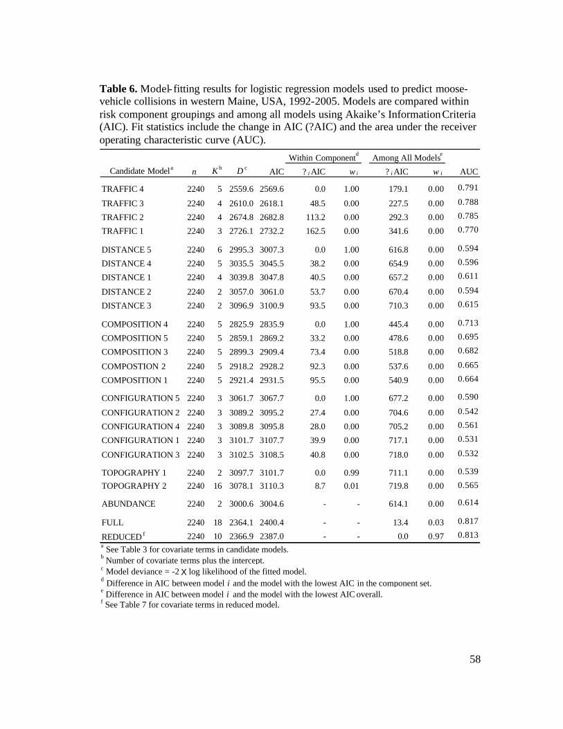
58

Table 6. Model-fitting results for logistic regression models used to predict moose-vehicle collisions in western Maine, USA, 1992-2005. Models are compared within risk component groupings and among all models using Akaike’s Information Criteria (AIC). Fit statistics include the change in AIC (?AIC) and the area under the receiver operating characteristic curve (AUC).

Candidate Modela n K b D c AIC ? i AIC w i ? i AIC w i AUC

TRAFFIC 4 2240 5 2559.6 2569.6 0.0 1.00 179.1 0.00 0.791

TRAFFIC 3 2240 4 2610.0 2618.1 48.5 0.00 227.5 0.00 0.788

TRAFFIC 2 2240 4 2674.8 2682.8 113.2 0.00 292.3 0.00 0.785

TRAFFIC 1 2240 3 2726.1 2732.2 162.5 0.00 341.6 0.00 0.770

DISTANCE 5 2240 6 2995.3 3007.3 0.0 1.00 616.8 0.00 0.594

DISTANCE 4 2240 5 3035.5 3045.5 38.2 0.00 654.9 0.00 0.596

DISTANCE 1 2240 4 3039.8 3047.8 40.5 0.00 657.2 0.00 0.611

DISTANCE 2 2240 2 3057.0 3061.0 53.7 0.00 670.4 0.00 0.594

DISTANCE 3 2240 2 3096.9 3100.9 93.5 0.00 710.3 0.00 0.615

COMPOSITION 4 2240 5 2825.9 2835.9 0.0 1.00 445.4 0.00 0.713

COMPOSITION 5 2240 5 2859.1 2869.2 33.2 0.00 478.6 0.00 0.695

COMPOSITION 3 2240 5 2899.3 2909.4 73.4 0.00 518.8 0.00 0.682

COMPOSTION 2 2240 5 2918.2 2928.2 92.3 0.00 537.6 0.00 0.665

COMPOSITION 1 2240 5 2921.4 2931.5 95.5 0.00 540.9 0.00 0.664

CONFIGURATION 5 2240 3 3061.7 3067.7 0.0 1.00 677.2 0.00 0.590

CONFIGURATION 2 2240 3 3089.2 3095.2 27.4 0.00 704.6 0.00 0.542

CONFIGURATION 4 2240 3 3089.8 3095.8 28.0 0.00 705.2 0.00 0.561

CONFIGURATION 1 2240 3 3101.7 3107.7 39.9 0.00 717.1 0.00 0.531

CONFIGURATION 3 2240 3 3102.5 3108.5 40.8 0.00 718.0 0.00 0.532

TOPOGRAPHY 1 2240 2 3097.7 3101.7 0.0 0.99 711.1 0.00 0.539

TOPOGRAPHY 2 2240 16 3078.1 3110.3 8.7 0.01 719.8 0.00 0.565

ABUNDANCE 2240 2 3000.6 3004.6 - - 614.1 0.00 0.614

FULL 2240 18 2364.1 2400.4 - - 13.4 0.03 0.817

REDUCED f 2240 10 2366.9 2387.0 - - 0.0 0.97 0.813

f See Table 7 for covariate terms in reduced model.

Among All ModelseWithin Componentd

b Number of covariate terms plus the intercept.

a See Table 3 for covariate terms in candidate models.

c Model deviance = -2 X log likelihood of the fitted model.d Difference in AIC between model i and the model with the lowest AIC in the component set. e Difference in AIC between model i and the model with the lowest AIC overall.

59

Table 7. Coefficient estimates from the reduced logistic regression model used to predict moose-vehicle collisions in

western Maine, USA, 1992-2005. I used a generalized estimating equation (GEE) approach to control for spatial

autocorrelation by grouping observations into clusters identified through kernel density analysis and to derive robust

standard errors for parameter estimates.

Parameter Standardized Estimate

SE Wald ?2 P > |?2| Odds Ratio 95% CI Unit Increase for Odds Ratio

INTERCEPT 0.5959a 0.7662 0.6084 0.4367

AADT 0.7622 0.0001 79.21 <0.0001 1.57 1.42, 1.73 500 (AADT)

CUT (2.5 km) 0.3261 0.0084 55.0564 <0.0001 1.36 1.26, 1.48 5 (%)

SPEED 0.1834 0.0181 10.89 <0.0001 1.35 1.13, 1.61 8 (km/hour)

CF (2.5 km) 0.0884 0.0150 5.2441 0.0220 1.19 1.02, 1.38 5 (%)

IJI (5 km) -0.0822 0.0125 3.8025 0.0516 0.89 0.78, 1.00 5 (%)

D_SHBWET -0.1349 0.0011 19.0096 <0.0001 0.96 0.94, 0.98 100 (m)

D_DEV 0.1636 0.0009 11.2225 0.0008 1.02 1.01, 1.04 100 (m)

AADT2 -0.4714 0.0001 16.5649 <0.0001

AADT X SPEED -0.1217 0.0006 1.6641 0.1972

a Non-standardized estimate.

60

Table 8. Validation results of logistic regression modeling used to predict moose-vehicle collisions (MVCs) in western Maine

and statewide, Maine, USA, 1992-2005. Validation accuracy was based on the percentage of correctly classified responses for

observations (0 = random controls, 1 = MVC) using a 0.5 probability cutoff. The area under the receiver operating

characteristic curve (AUC) is a measure of the discriminatory power of a model and ranges from 0.5 (model predictions no

better than chance) to 1.0 (best possible discriminatory power). See Table 7 for logistic regression model terms.

Validation Set n Sensitivity Specificity Overall AUC

Western Maine 742 75.4 74.7 75.0 0.835

Statewide 13,339 59.2 78.5 68.8 0.828

% Correct Classification

61

Figure 1. Locations of moose-vehicle collisions (MVCs) in western Maine, USA,

1992-2005.

62

0 25 50 75Kilometers

MVC (1992-2005)

Roads

Townships

Western Mountains Study Area

¹

NAD 1983 UTM Zone 19N

63

Figure 2. Density per km2 of (a) roads (km), (b) moose-vehicle collisions (MVCs),

and (c) hunter harvest of moose in townships of Maine, USA, 1992-2005. Shown are

boundaries delineating the western Maine study area and the portion of the state open

to moose hunting.

64

a) Road density

¹

b) MVC density

MVC / Sq. km< 0.001

0.001 - 0.06

0.06 - 0.19

0.19 - 6.52

Western Maine study area

Townships

Road km / Sq. km<0.0001

0.0001-0.31

0.31-0.90

0.90-42


Townships

0 30 60 90Km

Moose harvest / Sq. km< 0.001

0.001 - 0.02

0.02 - 0.04

0.04 - 0.22


Townships - moose hunting not permitted

c) Harvest density

65

Figure 3. Temporal distribution of moose-vehicle collisions (MVCs) in the western

Maine study area and statewide, Maine, USA, 1992-2005. (a) Percentage of

MVC/month, (b) percentage of MVC/daily time period, (c), annual frequency of

MVCs and moose harvested and (d) ratio of MVC to Harvest.

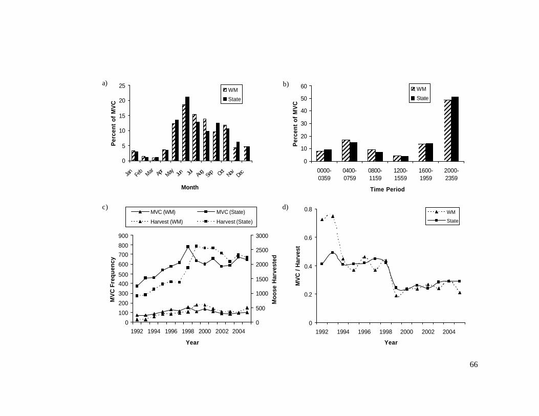
66

0

100

200

300

400500

600

700800

900

1992 1994 1996 1998 2000 2002 2004

Year

MV

C F

requ

ency

0

500

1000

1500

2000

2500

3000

Moo

se H

arve

sted

MVC (WM) MVC (State)

Harvest (WM) Harvest (State)

c)

0

0.2

0.4

0.6

0.8

1992 1994 1996 1998 2000 2002 2004

Year

MV

C /

Har

vest

WM

State

d)

0

10

20

30

40

50

60

0000-0359

0400-0759

0800-1159

1200-1559

1600-1959

2000-2359

Time Period

Per

cent

of

MV

C

WM

State

b)

0

5

10

15

20

25

Jan Feb Mar Ap

rMay Jun Jul Au

gSe

p OctNo

vDe

c

Month

Per

cent

of

MV

C

WM

State

a)

67

Figure 4. Plotted values of the L-statistic for network K-function analysis of moose-

vehicle collisions (MVCs) in western Maine, USA, 1992-2005. The statistic L(t)

(dark black line) represents the observed number of neighboring MVCs per MVC

within distance t along the road network. Positive values of L(t) indicate clustering

and negative values indicate regular dispersion. A 95% confidence envelope

generated by 100 Monte Carlo simulations (light gray lines) surrounds the expected

value of L(t), which is zero for a random point distribution. Values of L(t) within the

confidence interval indicate a random point distribution.

68

-20

-10

0

10

20

30

0 10 20 30 40 50 60

Distance t (km)

L(t

)

L(t)Upper 95% CILower 95% CI

69

Figure 5. Fixed kernel density estimations of moose-vehicle collisions in western

Maine, USA, 1992-2005. Bandwidths (smoothing parameters) used to calculate

kernel density were (a) 1 km, (b) 5 km, and (c) 10 km. (a) Section of road in Franklin

County, Maine, used to illustrate kernel density clusters for MVCs derived using a

1-km search radius.

70

0 3 6 9kilometers

0 50Kilometers

a) 1-km bandwidth

b) 5-km bandwidth c) 10-km bandwidth

Kernel Range010 %

20 %

30 %

40 %50 %

60 %70 %

80 %

90%

Western Maine

71

Figure 6. Clusters of moose-vehicle collisions (MVCs) and random points identified

through kernel density analysis in western Maine, USA, 1992-2005. The clusters

were used to group observations in a general estimating equation (GEE) logistic

regression model in order to account for spatial dependence among observations.

Clusters were delineated using the 50% contour from the kernel estimation with a 1-

km search radius. Shown is a portion of State Highway 6/15 between Jackman and

Moosehead Lake in Somerset and Piscataquis Counties, Maine.

72

0 1 2 30.5Kilometers

¹

Random Control

MVCKernel density 50% contour (GEE model cluster value)

State Highway 6/15

73

Figure 7. Predicted probability of moose-vehicle collisions against landscape

predictor covariates, western Maine, USA, 1992-2005. Output was derived from a

final reduced logistic regression model (see Table 7). I used a loess smoother

(Minitab 2005) to smooth predicted probability across all observations.

74

Pre

dic

ted

Pro

babi

lity

of M

VC

908070605040

1.0

0.5

0.0

100007500500025000 403020100

302520151050 706560555045 100007500500025000

1.0

0.5

0.0

40003000200010000

1.0

0.5

0.0

a) SPEED (km/hour) b) Traffic Volume (AADT) c) CUT (2.5 km)

d) CF (2.5 km) e) IJI (5 km) f) D_DEV (m)

g) D_SHBWET (m)

75

Figure 8. Predicted probability of moose-vehicle collisions agains t traffic volume

(AADT) shown by level of speed limit (SPEED), western Maine, USA, 1992-2005.

Output was derived from a final reduced logistic regression model (see Table 7).

Different probabilities for high and low speed limits reflect an interaction between

SPEED and AADT. I used a loess smoother (Minitab 2005) to smooth predicted

probability across all observations.

76

Annual average daily traffic volume (AADT)

Pre

dic

ted

Pro

ba

bil

ity

of

MV

C

120001000080006000400020000

1.0

0.8

0.6

0.4

0.2

0.0

High (>72 km/hour)Low (<72 km/hour)

SPEED LEVEL

77

Figure 9. Mean values of land cover composition covariates calculated within buffers

surrounding moose-vehicle collisions (MVCs) and random points in western Maine,

USA, 1992-2005. (a) Percent cutover forest, (b) percent non-woody wetland, (c)

percent coniferous forest, (d) percent deciduous-mixed forest, (e) edge density

(m/ha), (f) Simpson’s diversity index (range = 0-1). Buffer radii were 0.25, 0.5, 1.0,

2.5, and 5.0 km. Bars represent 95% confidence intervals for the mean.

78

d) % Deciduous-mixed forest

0

10

20

30

40

50

60

70

0.25 0.50 1.00 2.50 5.00

Per

cent

b) % Non-woody wetland

0

5

10

15

20

25

0.25 0.50 1.00 2.50 5.00

Per

cent

a) % Cutover forest

0

5

10

15

20

25

0.25 0.50 1.00 2.50 5.00

Per

cent

MVC Random

c) % Coniferous forest

0

5

10

15

20

25

0.25 0.50 1.00 2.50 5.00

Per

cent

e) Edge density (m/ha)

100

120

140

160

180

200

220

240

0.25 0.50 1.00 2.50 5.00

Buffer radius (km)

m /

ha

f) Simpson's diversity index

0.5

0.6

0.7

0.8

0.9

0.25 0.50 1.00 2.50 5.00

Buffer radius (km)

Inde

x (0

-1)

79

Figure 10. Mean or proportional values of land cover configuration covariates

calculated within buffers surrounding moose-vehicle collisions (MVCs) and random

points in western Maine, USA, 1992-2005. (a) Patch area, (b) interspersion-

juxtaposition index, (c) terrain ruggedness (standard deviation [SD] of elevation), (d)

aspect (proportion of observations). Buffer radii were 0.25, 0.5, 1.0, 2.5, and 5.0 km.

Bars represent 95% confidence intervals for the mean.

80

a) Patch area

0

2

4

6

8

10

12

0.25 0.50 1.00 2.50 5.00

Buffer radius (km)

Hec

tare

sMVC Random

b) Interspersion-juxtaposition index

52

56

60

64

68

0.25 0.50 1.00 2.50 5.00

Buffer radius (km)

IJI (

0-10

0)

c) Mean ruggedness

0

20

40

60

80

100

0.25 0.50 1.00 2.50 5.00

Buffer radius (km)

SD

of

elev

atio

n (

m)

d) Aspect

0

5

10

15

20

N NE E SE S SW W NW

Aspect

Per

cen

t

81

APPENDIX A. Calculation of human population density in Maine using 2000

Census Bureau data.

I obtained data for the human population of Maine based on estimates from

the 2000 United States Census. These data were obtained within a polygon shapefile

(mcdccd00.shp ; MEGIS 2002) that depicted population by Minor Civil Division

(MCD) or Census County Division (CCD) boundaries at 1:100,000 scale; these

divisions represent counties, census sub-areas, minor civil divisions, and unorganized

territories and were defined by the Census Bureau to enable reporting over large,

predominately rural areas (MEGIS 2002). In addition, I obtained a polygon shapefile

(biophy.shp; MEGIS 1991) depicting the 15 “biophysical” regions of Maine, as

classified by McMahon (1990).

To derive a statewide population density estimate, I used ArcMap (ESRI

2004) to calculate the mean for population density (population/polygon area [km2])

across all polygons. To derive a regional population density estimate for western

Maine, I used the Polygon In Polygon Analysis tool within the Hawth’s Tools

extension of ArcMap (Beyer 2004) to calculate the area-weighted mean for

population density. The area-weighted mean was based on the proportion of each

census division feature in mcdccd00.shp that intersected the Western Mountains

feature (representing the “western Maine” study area) in biophy.shp. Accounting for

the area of individual census divisions within the western Maine region was necessary

because there was no 1-to-1 relationship between census divisions (i.e.,

mcdccd00.shp) and the region (biophy.shp).

82

APPENDIX B. Description of the K-function and network K-function.

The traditional K-function (Ripley 1981) uses the Euclidean distance between

all points of interest, within the 2-dimensional spatial extent of the study area, to

calculate the number of neighboring points within a specified radial distance

increment t of each point in the data set. The distance increments t can be thought of

as the radii of concentric circles placed over each point i, such that the cumulative

number of points j occurring within t is counted (Bailey and Gatrell 1995). By

specifying multiple t, the user can determine the relative distribution of points (i.e.,

random, regular, or clustered) across several scales. Under the null hypothesis of

complete spatial randomness (CSR), points are randomly distributed such that the

expected K-function is

K(t) = p X t2 [1]

for all values of t. CSR serves as a baseline against which the observed patterns can

be tested for clustering, regular dispersion, or randomness (Bailey and Gatrell 1995).

Where points are not distributed randomly, the observed K-function is

? ??? ?

?n

jii

n

j ij

ijt

w

dI

nR

tK1 1

2

)()(ˆ [2]

where R is the 2-dimensional area of the study region, n is sample size, dij is the

distance from MVC i to MVC j, It is an indicator function equal to 1 if dij = t or 0

otherwise, and wij is the conditional probability that an event is observed within R (an

edge correction term; Bailey and Gatrell 1995).

83

The traditional K-function may not be appropriate for points that occur only

along linear networks (e.g., roads; Spooner et al. 2004). Okabe and Yamada (2001)

developed a modified version of the K-function that handles points p (p1,…,pn)

distributed along a network. The network is defined by network links RLT and a total

network length | RLT |. The expected network K-function is defined as

???1

)( networktK (points of P within network distance t of pi) [3]

where E(.) is the expected value for points P, which are assumed to follow a binomial

point distribution; ? is the density of points P on the network, such that ? = n / | RLT |

(Spooner et al. 2004). The null hypothesis for points P is a uniform and independent

distribution over the network. If the null is rejected, then points P are spatially

interacting and may be either clustered or regularly dispersed. From [3], the observed

network K- function is calculated as

???

?n

i

Tnetwork nn

RLtK

1)1(||

)(ˆ (points of P on RLp(t)) [4]

where RLp is a specific road link within | RLT |.

84

VITA

NAME: Zachary David Danks

DATE OF BIRTH: 6 October 1981

PLACE OF BIRTH: Russellville, KY

EDUCATION: Name and Location Dates Degree

High School: Logan County H. S., 1996-2000 Russellville, KY College: University of Kentucky, 2000-2004 B.S., Natural College of Agriculture, Resource Lexington, KY Conservation and Management Graduate School: State University of New 2004-2007 M.S., York (SUNY), College of Environmental Environmental Science and Forest Biology & Forestry (ESF), (Wildlife Biology Syracuse, NY and Management) EMPLOYMENT: Employer Dates Job Title SUNY-ESF, 2006-2007 Instructional Adirondack Ecological Support Assistant / Center, Webb Apprentice Newcomb, NY Elk Lake Lodge, Inc. 2006 Ecological Intern North Hudson, NY The Research Foundation 2006 Research Assistant of SUNY, Syracuse, NY SUNY-ESF 2004-2006 Teaching Assistant Syracuse, NY University of Kentucky, 2003, 2004 Research Department of Forestry Technician Lexington, KY Holland Employment, 2001, 2002 Equipment operator Logan Aluminum, Inc. Russellville, KY

danks ms thesis 2007

Documents