data, assumptions and methodology

1

Copyright © 2018 Siemens Industry. All Rights Reserved. DRAFT-SUBJECT TO SUBSTANTIAL CHANGES

MEMO TO: PREPA IRP Team

FROM: Siemens PTI/EBA

DATE: August 21, 2018

SUBJECT: PREPA IRP Load Forecast

The aim of this section is to present and discuss the gross electricity demand forecast (e.g. before any adjustments

for future energy efficiency, demand response or distributed generation, which will be modeled separately and are

provided in another memo), prepared as required for the development of the Integrated Resource Plan (IRP) for

PREPA. This includes a concise presentation of the data used, a description of the methodology and the necessary

assumptions, and finally the resulting load forecast. The forecast has been prepared for the IRP study horizon of

fiscal year (FY) 2019-2038 (July 1, 2018 – June 30, 2038).

Data, Assumptions and Methodology

Historical Energy Sales

Siemens used monthly historical energy sales provided by PREPA for the econometric model used to develop the

load forecast. Siemens used data for fiscal years (FY) 2000-2018 (July 1999 - June 2018) broken down into six

customer classes; residential, commercial, industrial, agriculture, public lighting, and other. The commercial is the

largest sector accounting for 47% of the total sales in FY 2017, followed by residential (38%) and industrial (13%).

Overall, the combined sales to residential, commercial, and industrial customers represented 98% of the total in FY

2017, with the remaining 2% of sales coming mostly from the public lightning sector.

Electricity sales in Puerto Rico declined 18% since the Great Recession due to a structural decline in the economy

and net migration of people out of the island with GNP and population falling by at least a percentage point annually

since 20071. For FY 2018, total sales declined 22%, reflecting the disruption in the transmission and distribution

networks due to the hurricanes as well as customer billing delays2.

Industrial sales declined 47% in FY 2007-2017, while residential and commercial fell 12% and 10%, respectively.

Industrial share of the total demand declined from 20% in FY 2007 to 13% in FY 2017. In contrast, the share of

commercial sales increased by 4 percentage points during the same period. Exhibit 1 shows historical energy sales

for fiscal years 2000-2017 by customer class, as reported by PREPA.

1 The prior six years 2000 to 2006 saw an average growth in the GNP of 1.4% yearly while the broader US economy

saw a growth of 2.6%. 2 Based on preliminary data provided by PREPA

2


Exhibit 1: Historical PREPA Annual Sales by Customer Class (GWh)

Source: PREPA

Energy sales were normalized for each of the six customer classes. PREPA indicated that historical sales can be

affected by billing issues (delays, incorrect reporting, etc.), which might explain high volatility for some months, not

in line with changes in monthly generation on a system wide basis. The volatility is particularly notorious after

hurricanes Irma and Maria struck Puerto in the fall of 2017, with extreme volatility and low or even negative energy

monthly sales numbers reported after September 2017. PREPA indicated, the Company is still in the process of

validating data and making corrections for reported sales post Maria. For this reason, Siemens did not include

historical numbers for fiscal year 2019 as part of the econometric regression analysis.

To correct for abnormal data volatility and avoid biases embedded in the forecast results, Siemens normalized the

sales data by customer class using historic monthly generation and the relative share of each class to the total net

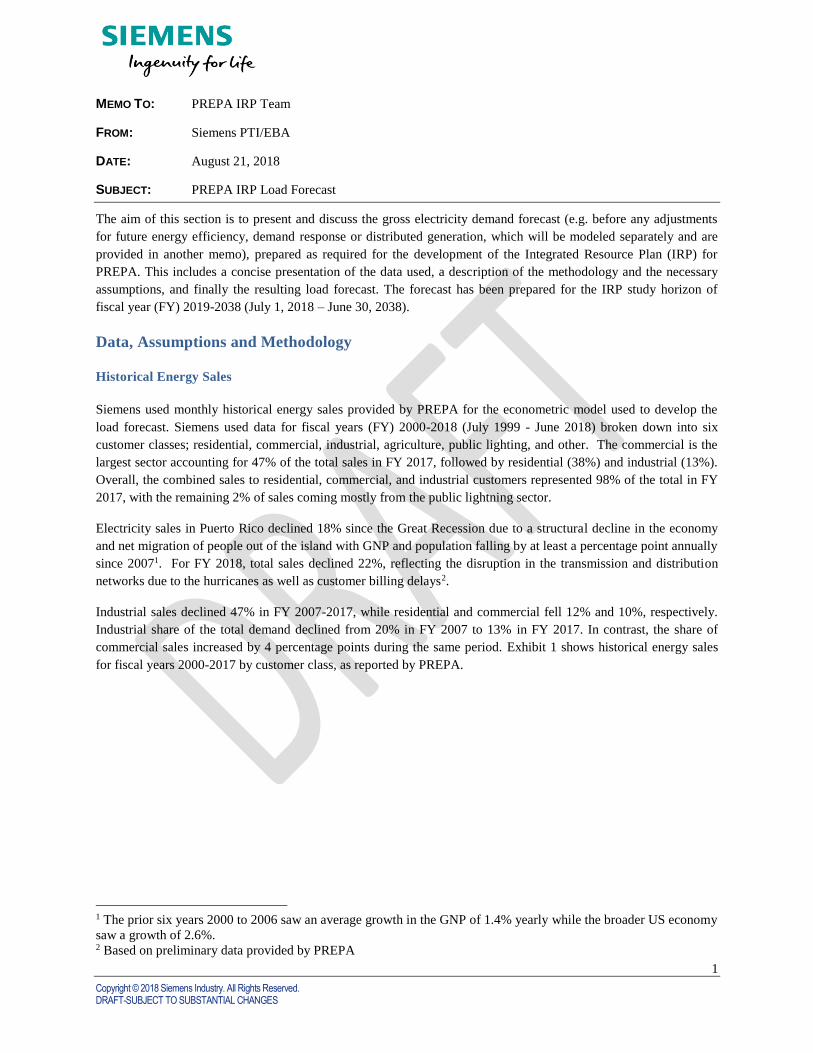
generation reported. Exhibit 2 shows the normalization for the industrial customer class compared to the raw data

and the net system generation for 2012-2014. The chart shows the normalization technique eliminated unexplained

volatility in months such as May or June 2012, and the rise or fall in monthly sales not following net generation

levels. The normalized data was used for the econometric regression analysis described next.

3


Exhibit 2: Historical Normalized data for the Industrial Customer Class

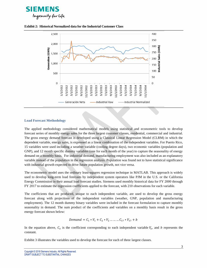
Load Forecast Methodology

The applied methodology considered mathematical models using statistical and econometric tools to develop

forecast series of monthly energy sales for the three largest customer classes, residential, commercial and industrial.

The gross energy demand forecast is developed using a Classical Linear Regression Model (CLRM) in which the

dependent variable, energy sales, is expressed as a linear combination of the independent variables. For Puerto Rico,

15 variables were used including a weather variable (cooling degree days), two economic variables (population and

GNP), and 12 month specific dummy variables (one for each month of the year) to capture the seasonality of energy

demand on a monthly basis. For industrial demand, manufacturing employment was also included as an explanatory

variable instead of the population in the regression analysis. Population was found not to have statistical significance

with industrial growth expected to drive future population growth, not vice versa.

The econometric model uses the ordinary least-squares regression technique in MATLAB. This approach is widely

used to develop long-term load forecasts by independent system operators like PJM in the U.S. or the California

Energy Commission in their annual load forecast studies. Siemens used monthly historical data for FY 2000 through

FY 2017 to estimate the regression coefficients applied to the forecast, with 210 observations for each variable.

The coefficients that are produced, unique to each independent variable, are used to develop the gross energy

forecast along with projections of the independent variables (weather, GNP, population and manufacturing

employment). The 12 month dummy binary variables were included in the forecast formulation to capture monthly

seasonality in demand. The sum product of the coefficients and variables on a monthly basis result in the gross

energy forecast shown below:

𝐷𝑒𝑚𝑎𝑛𝑑 = 𝐶1 ∗ 𝑉1 + 𝐶2 ∗ 𝑉2 … … … 𝐶17 ∗ 𝑉17 + 𝑏

In the equation above, 𝐶𝑥 is the coefficient corresponding to each independent variable 𝑉𝑥, and b represents the

constant.

Exhibit 3 illustrates the variables used to develop the forecast for each of three largest classes.

4


Exhibit 3: Independent variables for Each Customer Classes

The statistical significance of the explanatory variables and predicted fit of the model for each class was robust, as

shown in Exhibit 4 for the residential class. The predicted values followed monthly historical sales to a great extent.

The regression coefficients, adjusted R2s, and F-stats from the econometric model for each class are shown in

Appendix A.

Exhibit 4: Residential Class Predicted Fit vs. Actuals

Source: PREPA, Siemens

For the smaller customer classes (agriculture, lighting and other) the overall fit of the CLRM model was not as

robust with the economic and weather fundamental variables providing a much lower explanatory value on the

energy demand for each class. For these customer classes, Siemens developed the forecast based on their historical

seasonality and using a simpler extrapolation technique with the expectation that each class follow similar growth

rates to the overall system.

Fundamental Drivers for the Load Forecast

In line with the econometric model, Siemens used population, GNP, CDD and the monthly dummy variables as

explanatory variables to develop the load forecast by customer class for FY 2019-2038. Other economic data was

considered, including disposable income, income per-capita, and the heat index for weather but they were not

included due to its high correlation to other variables already incorporated in the analysis such as CDD (highly

correlated to the heat index) or the GNP (highly correlated to disposable income), diluting their predictive value.

Residential

• CDD

• GNP

• Population

• 12 month variables

Commercial

• CDD

• Population


Industrial

• CDD

• GNP

• Manufacturing Employment


5


For weather data, Siemens found Cooling Degree Days as the most statistically significant variable to predict the

impact of weather on load, despite Puerto Rico having a tropical climatic zone with warm temperatures all year

round averaging 80°F (27°C) in low elevation areas, and 70°F (21°C) in the lush central mountains of the island.

Although temperature variation is relatively modest throughout the year, the overall heat level drives cooling load

trends (demand for air conditioning). Weather data was sourced from the National Oceanic and Atmospheric

Association (NOAA) for the San Juan station, as a representative for the overall island temperature and rainfall

trends. Higher elevation locations were not found to have a significant impact on overall load changes.

Customer rates were considered in the analysis, in particular industrial rates, but they were found not to have a

strong historic correlation to demand and explanatory power. In 2000 to 2017, there were periods where industrial

demand fell along with declining industrial rates or the opposite. The expectation would be an inverse relationship

with lower demand as a consequence of rising industrial rates. The manufacturing sector in Puerto Rico, mostly

comprised of pharmaceutical, textiles, petrochemicals, and electronics; appears to be less responsive to changes in

customer rates compared to other manufacturing industries such as steel or aluminum, which are highly sensitive

(high elasticity). The residential sector is traditionally a sector with low response to changes in retail rates and to

some extend the commercial customers. However, sustained high retail rates could change customer behavior and

create more incentives for implementation of energy efficiency programs.

Siemens compiled and reviewed macroeconomic data (historical and forecasts) from several sources including

Moody’s Analytics, the International Monetary Fund, World Bank, the U.S. Census Bureau, Federal Reserve of

Economic Data of St. Louis (FRED) and Puerto Rico’s Federal Management Oversight Board (FOMB), among

others.

Exhibit 5 below shows the historical annual values for the independent variables used in the regression analysis.

Exhibit 5: Historical Population, Macroeconomic, and Weather Variables

Year Population

(thousands)

GNP

(Real Million US dollars)

Cooling Degree Days

(Monthly Average)

Manufacturing Employment

(thousands)

2000

2001

2002

2003

2004

2005

2006

2007

2008

2009

2010

2011

2012

2013

2014

2015

2016

2017

3,815

3,822

3,825

3,827

3,825

3,814

3,794

3,772

3,750

3,733

3,702

3,656

3,615

3,566

3,504

3,441

3,372

3,190

6,773

6,873

6,850

6,991

7,178

7,315

7,351

7,262

7,054

6,784

6,542

6,432

6,466

6,458

6,348

6,312

6,209

6,060

453

476

477

472

461

478

473

489

467

499

491

462

506

496

519

513

506

504

143

132

121

118

118

115

110

106

101

92

87

84

82

76

75

74

74

72

Source: FOMB (GNP), Moody’s (Population), NOAA (weather), FRED (Manufacturing Employment)

Before the hurricane, Puerto Rico’s economy was in structural decline, with GNP and population falling by at least a

percentage point a year since 2006, the last year when the GNP saw an increase. Puerto Rico’s GNP shrunk 8% in

the decade after the Great Recession with GNP reaching $6 billion dollars in 2017 (real dollars).

6


Population declined 15% since 2007 with Maria and Irma accounting for 4 percentage points of this decline in

population (182 thousand people in 2017) due to the combined impact of migration and the death toll after the

storm, estimated at over 4,100 people3.

Macroeconomic and Weather Projections

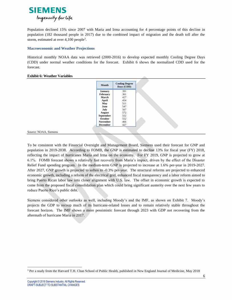
Historical monthly NOAA data was retrieved (2000-2016) to develop expected monthly Cooling Degree Days

(CDD) under normal weather conditions for the forecast. Exhibit 6 shows the normalized CDD used for the

forecast.

Exhibit 6: Weather Variables

Month Cooling Degree

Days (CDD)

January

February

March

April

May

June

July

August

September

October

November

December

391

361

427

454

511

547

567

572

552

552

466

427

Source: NOAA, Siemens

To be consistent with the Financial Oversight and Management Board, Siemens used their forecast for GNP and

population in 2019-2038. According to FOMB, the GNP is estimated to decline 13% for fiscal year (FY) 2018,

reflecting the impact of hurricanes Maria and Irma on the economy. For FY 2019, GNP is projected to grow at

6.1%. FOMB forecast shows a relatively fast recovery from Maria’s impact, driven by the effect of the Disaster

Relief Fund spending program. In the medium-term GNP is projected to increase at 1.6% per-year in 2019-2027.

After 2027, GNP growth is projected to soften to -0.3% per-year. The structural reforms are projected to enhanced

economic growth, including a reform of the electrical grid, enhanced fiscal transparency and a labor reform aimed to

bring Puerto Rican labor law into closer alignment with U.S. law. The offset in economic growth is expected to

come from the proposed fiscal consolidation plan which could bring significant austerity over the next few years to

reduce Puerto Rico’s public debt.

Siemens considered other outlooks as well, including Moody’s and the IMF, as shown on Exhibit 7. Moody’s

projects the GDP to recoup much of its hurricane-related losses and to remain relatively stable throughout the

forecast horizon. The IMF shows a more pessimistic forecast through 2023 with GDP not recovering from the

aftermath of hurricane Maria in 2017.

3 Per a study from the Harvard T.H. Chan School of Public Health, published in New England Journal of Medicine, May 2018

7


Exhibit 7: Puerto Rico GNP Forecasts

Note: The forecast have been standardized for comparison purposes using the implied growth rates. Moody’s GNP forecast is based on real

2009$ and the IMF based on real 1954$.

Sources: Moody’s June 2018 Forecast, IMF April 2018 WEO, Financial Oversight and Managing Board of Puerto Rico, Fiscal Plan April 2018

The FOMB forecast for population shows a decline of 5.8% in FY2018 due to hurricanes fatalities and net migration

out of the island. Over the study period, FOMB projects population to decline at 1.3% per-year in 2019-2038.

Population in Puerto Rico is projected to fall by over 900 thousand people by 2038. Moody’s projects a faster pace

of population loss over the next decade, compared to FOMB, as the island gets increasingly dragged into a negative

feedback loop whereby out-migration undermines the tax base and the provision of public services (which

deteriorated since Hurricane Maria), will engender more out-migration. The U.S. Census (prior to Maria) projects

higher population levels but still with a falling trend through the forecast. The IMF provides a forecast in between

the projections from FOMB and Moody’s.

8


Exhibit 8: Puerto Rico Population Forecast

Sources: Moody’s June 2018 Forecast, IMF April 2018 WEO, US Census Bureau August 2017

Exhibit 9 shows the long-term economic forecast used in the load forecast.

Exhibit 9: Macroeconomic Long Term Forecast

Fiscal

Year

Population

(thousands of people)

GNP

(Real Millions US dollars)

Manufacturing Employment

(thousands of people)

2018

2019

2020

2021

2022

2023

2024

2025

2026

2027

2028

2029

2030

2031

2032

2033

2034

2035

2036

2037

2038

3,143

3,104

3,084

3,039

2,995

2,951

2,910

2,871

2,833

2,794

2,756

2,718

2,681

2,644

2,609

2,575

2,541

2,508

2,476

2,445

2,414

5,251

5,573

5,632

5,707

5,792

5,873

5,941

5,991

6,029

6,041

6,038

5,984

5,949

5,922

5,897

5,877

5,862

5,852

5,847

5,846

5,849

70

69

70

70

70

70

71

71

71

72

72

73

73

74

74

75

75

76

77

77

78

Source: FOMB (population and GNP), Siemens for Manufacturing employment

9


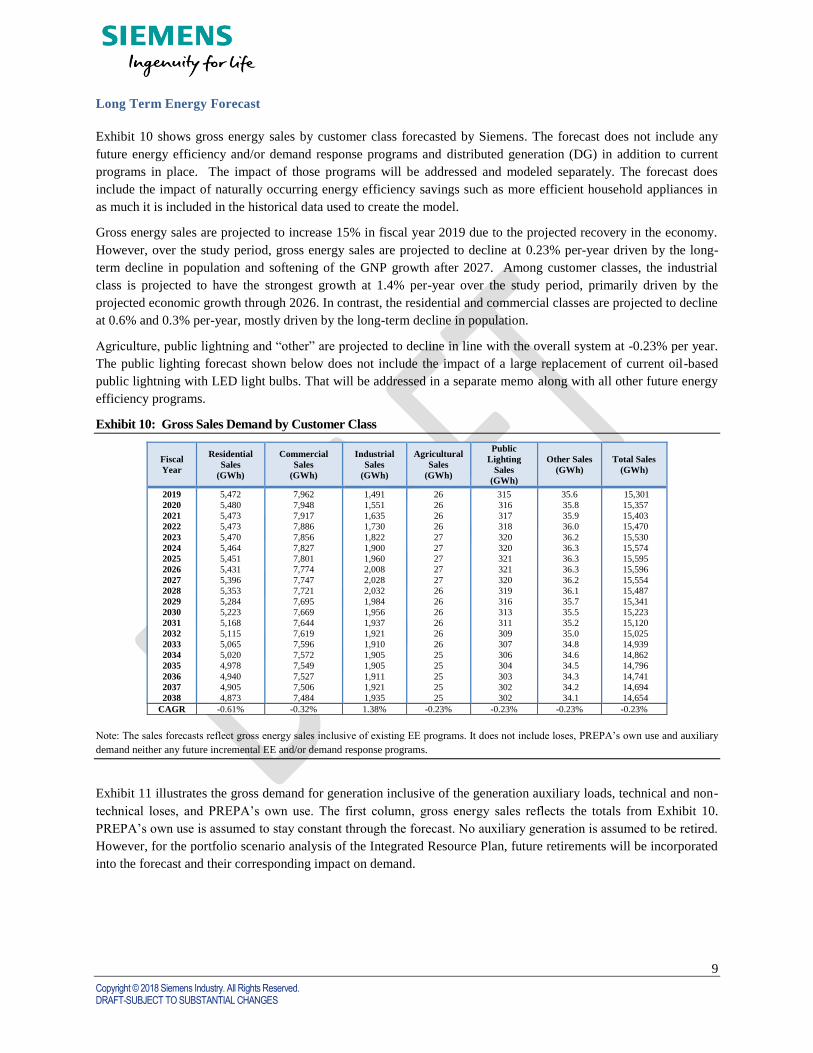
Long Term Energy Forecast

Exhibit 10 shows gross energy sales by customer class forecasted by Siemens. The forecast does not include any

future energy efficiency and/or demand response programs and distributed generation (DG) in addition to current

programs in place. The impact of those programs will be addressed and modeled separately. The forecast does

include the impact of naturally occurring energy efficiency savings such as more efficient household appliances in

as much it is included in the historical data used to create the model.

Gross energy sales are projected to increase 15% in fiscal year 2019 due to the projected recovery in the economy.

However, over the study period, gross energy sales are projected to decline at 0.23% per-year driven by the long-

term decline in population and softening of the GNP growth after 2027. Among customer classes, the industrial

class is projected to have the strongest growth at 1.4% per-year over the study period, primarily driven by the

projected economic growth through 2026. In contrast, the residential and commercial classes are projected to decline

at 0.6% and 0.3% per-year, mostly driven by the long-term decline in population.

Agriculture, public lightning and “other” are projected to decline in line with the overall system at -0.23% per year.

The public lighting forecast shown below does not include the impact of a large replacement of current oil-based

public lightning with LED light bulbs. That will be addressed in a separate memo along with all other future energy

efficiency programs.

Exhibit 10: Gross Sales Demand by Customer Class

Fiscal

Year

Residential

Sales

(GWh)

Commercial

Sales

(GWh)

Industrial

Sales

(GWh)

Agricultural

Sales

(GWh)

Public

Lighting

Sales

(GWh)

Other Sales

(GWh)

Total Sales

(GWh)

2019

2020

2021

2022

2023

2024

2025

2026

2027

2028

2029

2030

2031

2032

2033

2034

2035

2036

2037

2038

5,472

5,480

5,473

5,473

5,470

5,464

5,451

5,431

5,396

5,353

5,284

5,223

5,168

5,115

5,065

5,020

4,978

4,940

4,905

4,873

7,962

7,948

7,917

7,886

7,856

7,827

7,801

7,774

7,747

7,721

7,695

7,669

7,644

7,619

7,596

7,572

7,549

7,527

7,506

7,484

1,491

1,551

1,635

1,730

1,822

1,900

1,960

2,008

2,028

2,032

1,984

1,956

1,937

1,921

1,910

1,905

1,905

1,911

1,921

1,935

26

26

26

26

27

27

27

27

27

26

26

26

26

26

26

25

25

25

25

25

315

316

317

318

320

320

321

321

320

319

316

313

311

309

307

306

304

303

302

302

35.6

35.8

35.9

36.0

36.2

36.3

36.3

36.3

36.2

36.1

35.7

35.5

35.2

35.0

34.8

34.6

34.5

34.3

34.2

34.1

15,301

15,357

15,403

15,470

15,530

15,574

15,595

15,596

15,554

15,487

15,341

15,223

15,120

15,025

14,939

14,862

14,796

14,741

14,694

14,654

CAGR -0.61% -0.32% 1.38% -0.23% -0.23% -0.23% -0.23%

Note: The sales forecasts reflect gross energy sales inclusive of existing EE programs. It does not include loses, PREPA’s own use and auxiliary

demand neither any future incremental EE and/or demand response programs.

Exhibit 11 illustrates the gross demand for generation inclusive of the generation auxiliary loads, technical and non-

technical loses, and PREPA’s own use. The first column, gross energy sales reflects the totals from Exhibit 10.

PREPA’s own use is assumed to stay constant through the forecast. No auxiliary generation is assumed to be retired.

However, for the portfolio scenario analysis of the Integrated Resource Plan, future retirements will be incorporated

into the forecast and their corresponding impact on demand.

10


Exhibit 11: Gross Energy Demand for Generation

Fiscal

Year

Gross Energy

Sales

(GWh)

Technical

Losses

(GWh)

Non-Technical

Losses

(GWh)

Auxiliary

(GWh)

PREPA Own

Use

(GWh)

Total Energy

Demand

(GWh)

2019

2020

2021

2022

2023

2024

2025

2026

2027

2028

2029

2030

2031

2032

2033

2034

2035

2036

2037

2038

15,301

15,357

15,403

15,470

15,530

15,574

15,595

15,596

15,554

15,487

15,341

15,223

15,120

15,025

14,939

14,862

14,796

14,741

14,694

14,654

1,438

1,444

1,448

1,454

1,460

1,464

1,466

1,466

1,462

1,456

1,442

1,431

1,421

1,412

1,404

1,397

1,391

1,386

1,381

1,377

827

830

832

836

839

841

842

843

840

837

829

822

817

812

807

803

799

796

794

792

751

751

751

751

751

751

751

751

751

751

751

751

751

751

751

751

751

751

751

751

34

34

34

34

34

34

34

34

34

34

34

34

34

34

34

34

34

34

34

34

18,351

18,415

18,469

18,545

18,613

18,665

18,689

18,690

18,642

18,565

18,397

18,261

18,144

18,034

17,935

17,848

17,772

17,708

17,654

17,608

CAGR -0.23% -0.23% -0.23% 0.00% 0.00% -0.22%

To assess the geographical location of the demand above as necessary for the modeling of the system, PREPA

provided the composition of the load in term of customer classes (residential, commercial, industrial, etc.) by

County which was used to map the forecast to each of the areas into which the system is modeled. Exhibit 12 and

Exhibit 13show the resulting allocation of the Energy Demand for Generation above in tabular and graphic form.

Exhibit 12: Gross Energy Demand for Generation by Area

Fiscal

Year

ARECIBO

(GWh)

BAYAMON

(GWh)

CAGUAS

(GWh)

CAROLINA

(GWh)

MAYAGUEZ

(GWh)

PONCE ES

(GWh)

PONCE OE

(GWh)

SAN

JUAN

(GWh)

AUX

(GWh)

TOTAL

(GWh)

2,019 1,748 2,558 2,818 1,956 1,961 719 1,422 4,417 751 18,351

2,020 1,759 2,566 2,840 1,961 1,966 724 1,429 4,418 751 18,415

2,021 1,771 2,571 2,866 1,965 1,969 729 1,436 4,411 751 18,469

2,022 1,787 2,579 2,898 1,970 1,974 736 1,445 4,406 751 18,545

2,023 1,801 2,585 2,927 1,975 1,978 742 1,453 4,401 751 18,613

2,024 1,813 2,590 2,951 1,978 1,981 746 1,460 4,394 751 18,665

2,025 1,820 2,591 2,968 1,979 1,981 750 1,464 4,385 751 18,689

2,026 1,824 2,589 2,978 1,978 1,979 751 1,466 4,374 751 18,690

2,027 1,821 2,581 2,975 1,971 1,972 750 1,462 4,357 751 18,642

2,028 1,815 2,569 2,965 1,962 1,963 747 1,457 4,337 751 18,565

2,029 1,794 2,544 2,930 1,945 1,945 739 1,442 4,307 751 18,397

2,030 1,779 2,524 2,903 1,930 1,931 732 1,430 4,280 751 18,261

2,031 1,766 2,506 2,882 1,917 1,918 727 1,420 4,256 751 18,144

2,032 1,755 2,490 2,862 1,905 1,905 722 1,411 4,233 751 18,034

2,033 1,744 2,475 2,845 1,894 1,894 717 1,403 4,211 751 17,935

2,034 1,736 2,461 2,831 1,885 1,884 714 1,396 4,191 751 17,848

2,035 1,728 2,449 2,820 1,876 1,875 710 1,390 4,172 751 17,772

2,036 1,723 2,439 2,812 1,868 1,867 708 1,385 4,155 751 17,708

2,037 1,719 2,430 2,806 1,862 1,860 706 1,381 4,139 751 17,654

2,038 1,715 2,422 2,802 1,856 1,854 705 1,378 4,124 751 17,608

11


Exhibit 13: Graph of Gross Energy Demand for Generation by Area

Source: Siemens

Long Term Peak demand Forecast

To estimate the peak demand associated with the energy forecast it is necessary to determine for each customer class

their expected load factors (i.e. the ratio of average demand to the peak demand) and the percentage of their peak

demand that occurs at the time of the system peak (called Customer Class Coincidence Factor – CCCF - or

Contribution to the Peak Factor). These factors in principle should be determined monthly in line with the monthly

granularity of the energy forecast. However single values equal to the average of the determined monthly values was

preferred due to the fact that: a) there is not a significant change in the hourly load shapes for the relevant customer

classes across the year, b) the load factor can be volatile unless averages are made due to its dependence on the

measured peak and c) only one year worth of hourly load data by customer class was available.

Exhibit 14 shows the normalized load shapes for the main customer classes (Residential, Commercial and Industrial)

that make up most of the energy consumption as well as the system total. As can be observed, unlike the mainland

US where there are large changes in the shape from summer to winter, in Puerto Rico the shapes are largely the

same (residential shows the greater variation) and an average load factor can be used to represent each customer

class. We also note in the Exhibit below that there are two peaks a day time peak driven by commercial and

industrial loads and a night peak driven by the residential load and this is the higher of the two. Thus the residential

customers peak at the same time as the system (CCCF =1) while the industrial and commercial customers have a

lower peak at this time (CCCF < 1).

12


Exhibit 14: Normalized Load Shapes for main Customer Classes and System Total

Source: Siemens

Based on the hourly information provided Siemens estimated the load factors and Customer Class Coincidence

Factors (% of the Customer Class peak at the time of the System Peak) shown in Exhibit 15.

Exhibit 15: Selected Load Factors and Customer Class Coincidence Factor

Customer Class Load Factor Customer Class CF

% %

Residential 66.9% 100%

Commercial 70.2% 70%

Industrial 81.2% 85%

Lighting 49.3% 100%

Other 73.6% 80%

Agriculture 46.8% 32%

Source: Siemens

Using the values above and the forecasted energy consumption by customer class, the peaks demand and the

demand at the time of system peak can be determined. To this peak the following is added: a) effect of the technical

transmission and distribution technical loses using a correction to convert energy losses into capacity losses based

on the load factor4, b) non-technical loses using same values as the residential load, c) PREPA own consumption

using an estimated load factor based on historical values and b) finally the effect of the consumption of the

generating plants auxiliary services.

4 Capacity Losses % = (Energy Losses %) / (0.3+0.7*LF)

13


Exhibit 16 shows the gross average and peak demand for generation, inclusive of the factors indicated above

(technical and non-technical losses, auxiliary demand and PREPA’s own use). Exhibit 16 does not include the

impact of future energy efficiency and/or demand response programs or DG, which are modeled and addressed

separately.

Peak demand is projected to decline at 0.24% per year. The lower rate of peak growth relative to the energy demand

is a consequence of more modest growth in residential demand compared to commercial demand in the long-term

and the corresponding contribution of each class to peak demand. Commercial load peaks during the day, while the

residential peaks at night (sometimes very late), the last driving the system peak. A reduction in residential load

results in a reduction in the night peak and an increase in the overall system load factor.

Exhibit 16: Gross Average and Peak Demand for Generation

Fiscal

Year

Average Demand

(MW)

Peak Demand Load Factor

(%) (MW)

2019 2,095 2,791 75.1%

2020 2,102 2,799 75.1%

2021 2,108 2,805 75.2%

2022 2,117 2,815 75.2%

2023 2,125 2,823 75.3%

2024 2,131 2,829 75.3%

2025 2,133 2,831 75.3%

2026 2,134 2,830 75.4%

2027 2,128 2,822 75.4%

2028 2,119 2,810 75.4%

2029 2,100 2,785 75.4%

2030 2,085 2,765 75.4%

2031 2,071 2,748 75.4%

2032 2,059 2,731 75.4%

2033 2,047 2,716 75.4%

2034 2,037 2,703 75.4%

2035 2,029 2,692 75.4%

2036 2,021 2,682 75.4%

2037 2,015 2,673 75.4%

2038 2,010 2,666 75.4%

CAGR -0.22% -0.24%

Note: Forecast includes technical and non-technical losses, auxiliary demand and PREPA’s own use. The forecast does not include the impact of

future energy efficiency and/or demand response programs.

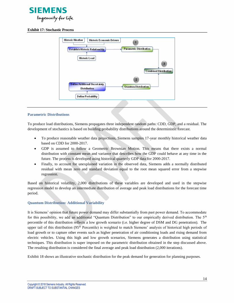
Stochastic Distribution

To generate scenarios for load growth, Siemens developed statistical distributions based on the deterministic load

forecasts. The process involves two steps, the first one, encompasses developing parametric distributions around the

key fundamental variables that could present more volatility in the future (weather and economic performance in

Puerto Rico) utilizing historical data to develop 2,000 scenarios for weather and GDP that are feed into the

econometric regression model to determine 2,000 iterations of average and peak load. The second step involves

developing Quantum distributions, which incorporate future uncertainties not captured by the historical data. The

overall process is summarized by the flow chart in Exhibit 17 below.

14


Exhibit 17: Stochastic Process

Parametric Distributions

To produce load distributions, Siemens propagates three independent random paths: CDD, GDP, and a residual. The

development of stochastics is based on building probability distributions around the deterministic forecast.

• To produce reasonable weather data projections, Siemens samples 17-year monthly historical weather data

based on CDD for 2000-2017.

• GDP is assumed to follow a Geometric Brownian Motion. This means that there exists a normal

distribution with constant mean and variance that describes how the GDP could behave at any time in the

future. The process is developed using historical quarterly GDP data for 2000-2017.

• Finally, to account for unexplained variation in the observed data, Siemens adds a normally distributed

residual with mean zero and standard deviation equal to the root mean squared error from a stepwise

regression.

Based on historical volatility, 2,000 distributions of these variables are developed and used in the stepwise

regression model to develop an intermediate distribution of average and peak load distributions for the forecast time

period.

Quantum Distribution: Additional Variability

It is Siemens’ opinion that future power demand may differ substantially from past power demand. To accommodate

for this possibility, we add an additional “Quantum Distribution” to our empirically derived distribution. The 5 th

percentile of this distribution reflects a low growth scenario (i.e. higher degree of DSM and DG penetration). The

upper tail of this distribution (95th Percentile) is weighted to match Siemens’ analysis of historical high periods of

load growth or to capture other events such as higher penetration of air conditioning loads and rising demand from

electric vehicles. Using this high and low growth scenarios, Siemens generates a distribution using statistical

techniques. This distribution is super imposed on the parametric distribution obtained in the step discussed above.

The resulting distribution is considered the final average and peak load distribution (2,000 iterations).

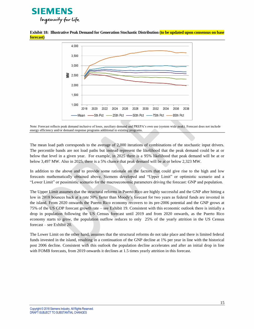
Exhibit 18 shows an illustrative stochastic distribution for the peak demand for generation for planning purposes.

15


Exhibit 18: Illustrative Peak Demand for Generation Stochastic Distribution (to be updated upon consensus on base

forecast)

Note: Forecast reflects peak demand inclusive of loses, auxiliary demand and PREPA’s own use (system wide peak). Forecast does not include energy efficiency and/or demand response programs additional to existing programs.

The mean load path corresponds to the average of 2,000 iterations of combinations of the stochastic input drivers.

The percentile bands are not load paths but instead represent the likelihood that the peak demand could be at or

below that level in a given year. For example, in 2025 there is a 95% likelihood that peak demand will be at or

below 3,497 MW. Also in 2025, there is a 5% chance that peak demand will be at or below 2,323 MW.

In addition to the above and to provide some rationale on the factors that could give rise to the high and low

forecasts mathematically obtained above, Siemens developed and “Upper Limit” or optimistic scenario and a

“Lower Limit” or pessimistic scenario for the macroeconomic parameters driving the forecast: GNP and population.

The Upper Limit assumes that the structural reforms in Puerto Rico are highly successful and the GNP after hitting a

low in 2018 bounces back at a rate 50% faster than Moody’s forecast for two years as federal funds are invested in

the island. From 2020 onwards the Puerto Rico economy recovers to its pre-2006 potential and the GNP grows at

75% of the US GDP forecast growth rate – see Exhibit 19. Consistent with this economic outlook there is initially a

drop in population following the US Census forecast until 2019 and from 2020 onwards, as the Puerto Rico

economy starts to grow, the population outflow reduces to only 25% of the yearly attrition in the US Census

forecast – see Exhibit 20.

The Lower Limit on the other hand, assumes that the structural reforms do not take place and there is limited federal

funds invested in the island, resulting in a continuation of the GNP decline at 1% per year in line with the historical

post 2006 decline. Consistent with this outlook the population decline accelerates and after an initial drop in line

with FOMB forecasts, from 2019 onwards it declines at 1.5 times yearly attrition in this forecast.

16


Exhibit 19: GNP Scenarios

Source: Siemens

Exhibit 20: Population Scenarios

Source: Siemens

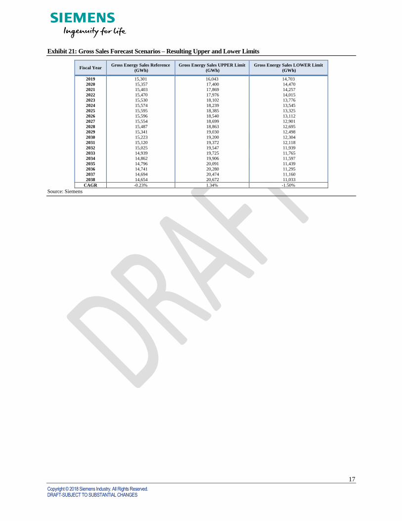
The resulting gross sales forecasts for the Upper and Lower limits are shown in Exhibit 21. In the high case

scenario, gross energy sales increase at 1.34% per-year, with sales reaching 20,672 GWh by 2038 – 41% higher than

the reference case. In the low case scenario, gross energy sales decline at 1.50% per-year reaching 11,033 GWh by

2038, 75% below the reference case level. The industrial customer class has the most upside or downside potential

driven by changes in the GNP and or population from all three classes, with sales growing at 5.6% per-year in the

high case, or declining at 5.2% per-year in the low case.

17


Exhibit 21: Gross Sales Forecast Scenarios – Resulting Upper and Lower Limits

Fiscal Year Gross Energy Sales Reference

(GWh)

Gross Energy Sales UPPER Limit

(GWh)

Gross Energy Sales LOWER Limit

(GWh)

2019

2020

2021

2022

2023

2024

2025

2026

2027

2028

2029

2030

2031

2032

2033

2034

2035

2036

2037

2038

15,301

15,357

15,403

15,470

15,530

15,574

15,595

15,596

15,554

15,487

15,341

15,223

15,120

15,025

14,939

14,862

14,796

14,741

14,694

14,654

16,043

17,400

17,869

17,976

18,102

18,239

18,385

18,540

18,699

18,863

19,030

19,200

19,372

19,547

19,725

19,906

20,091

20,280

20,474

20,672

14,703

14,470

14,257

14,015

13,776

13,545

13,325

13,112

12,901

12,695

12,498

12,304

12,118

11,939

11,765

11,597

11,439

11,295

11,160

11,033

CAGR -0.23% 1.34% -1.50%

Source: Siemens

18


Appendix A

Econometric Model Regression Coefficients by Customer Class

Residential

Variable Coefficient Statistical

Significance

Constant

CDD

GNP

Population

Jan

Feb

Mar

Apr

May

Jun

Jul

Aug

Sep

Oct

Nov

Dec

-227.36

0.366

0.047

91.083

-50.592

-84.916

-64.889

-67.875

-36.025

-32.552

-22.369

0.000

-31.389

-15.618

-42.071

-26.040

Yes

Yes

Yes

Yes

Yes

Yes

Yes

Yes

Yes

Yes

Yes

Yes

Yes

Yes

Yes

Adjusted R2 0.822

F-Stat 824.8

Commercial


Significance

Constant

CDD

Population

Jan

Feb

Mar

Apr

May

Jun

Jul

Aug

Sep

Oct

Nov

Dec

278.1

0.456

57.583

-23.315

-43.672

-2.185

-22.364

-13.705

-25.823

-26.560

0.000

-26.452

15.459

-10.917

1.679

Yes

Yes

Yes

Yes

Yes

Yes

Yes

Yes

Yes

Yes

Yes

Yes

Yes

Yes

Adjusted R2 0.587

F Stat 23.9

19


Industrial


Significance

Constant

CDD

GNP

Jan

Feb

Mar

Apr

May

Jun

Jul

Aug

Sep

Oct

Nov

Dec

Manufacturing

Employment

-532.88

0.11

0.09

-13.98

-25.86

-4.49

1.21

11.30

-0.31

1.32

2.89

-11.79

-3.09

-9.52

0.42

1.62

Yes

Yes

Yes

Yes

No

No

Yes

No

No

No

Yes

No

Yes

No

Yes

Adjusted R2 0.969

F Stat 434.71

data, assumptions and methodology

Documents