dc power ﬂow in rectangular coordinates -...

DC power flow in rectangular coordinates

Ross BaldickThe University of Texas, Austin, TX 78712

[email protected] 20, 2013

Title Page ◀◀ ▶▶ ◀ ▶ 1 of 21 Go Back Full Screen Close Quit

Abstract“DC power flow” is an analogy between approximations to the real powercomponents of the power flow equations and a direct current resistive circuit. Itcan also be interpreted as linearization of the real power components expressedin terms of phasor voltage magnitude and phase, linearized about a “flat start.”The accuracy of DC power flow for estimating real power flow is surprisinglygood in many cases, although it has large errors in some cases.We explore linearization of both the real and reactive powerequations expressedin terms of real and imaginary parts of the voltage phasor. Wefocus onlinearization about a flat start, which in rectangular coordinates has the voltagephasors each with real part one per unit and imaginary part zero.The resulting approximation has relatively good performance for real power.Because of the analog with linearization in terms of polar voltage representation,we call this approximation “DC power flow in rectangular coordinates.” We alsoexhibit an exact solution to the power flow equations for the particular case of alossless network.Keywords DC power flow, linearization.


1 Introduction∙ Exact or approximate solution of the power flow equations is essential to

the planning, operation, and control of power systems.∙ DC power flow [1, §4.1.4][2] is an analogy between an approximation to

the real power components of the AC power flow equations and a relateddirect current circuit:– can be interpreted as linearization of the real power components in terms

of phasor voltage magnitude and phase, that is, “polar coordinates,”– linearization is about a “flat start,” where the voltage phasors each have

magnitude one per unit and angle zero [3].∙ Most day-ahead locational electricity markets use DC powerflow [4] or

linearization.


1.1 Accuracy of DC power flow using polar coordinates∙ DC power flow is accurate for real power flow, except when:

– angle differences across lines are large, or– voltage magnitudes deviate significantly from one per unit [3, 5, 6].

∙ Precisely the most important conditions for evaluating limits, particularlypost-contingency limits!

∙ Linearization for reactive power in terms of polar coordinates is poor.


1.2 Rectangular coordinates∙ Recent significant progress in power flow and optimal power flow (OPF)

has used phasor voltage real and imaginary parts:– “rectangular coordinates” [7, 8, 9].

∙ Semi-definite programming formulations of the OPF problem usingrectangular coordinates have provided provably optimal solutions [10]:– may become the dominant approach to OPF.

∙ Linearization still standard currently in online applications.∙ Consider linearization in rectangular coordinates.


2 Formulation∙ v ∈ ℂ

n is the vector of complex phasor voltages at alln buses in thetransmission system,

∙ i ∈ ℂn is the vector of complex current injections into the transmission

system,∙ s ∈ ℂ

n is the vector of complex power injections into the transmissionsystem.

∙ Representv in rectangular coordinates by writing:

v = 1+ e+ j f ,

where:1 is the vector of all ones,e, f ,∈ ℝ

n, andj is the square root of minus 1.

∙ Define a “flat start” to bev = 1, corresponding toe = f = 0.


Formulation, continued∙ Y = G+ jB is the bus admittance matrix for the system:

– Off-diagonal entries are equal to minus the admittance of thecorrespondingseries elements joining corresponding buses,

– Diagonal entries are the sum of the admittances joined to thecorresponding buses, due to both series andshunt elements.

G = Gseries+Gshunt,

B = Bseries+Bshunt,

where:GshuntandBshuntare diagonal,GseriesandBseriesare symmetric (putting aside cases such as where

transformers have off-nominal turns ratios), andGseries1= Bseries1= 0, where0 is the vector (or depending on

interpretation, matrix) of all zeros.– AssumeGshunt= 0.


Formulation, continued∙ Kirchhoff’s current law:

i = Y v,= (G+ jB)(1+ e+ j f ),

= (Gseries+Gshunt+ j(Bseries+Bshunt))(1+ e+ j f ),

= (Gseries+ j(Bseries+Bshunt))(1+ e+ j f ), sinceGshunt= 0,

= Gseries1+Gseriese− (Bseries+Bshunt) f

+ j(Gseriesf +Bseries1+Bseriese+Bshunt1+Bshunte),

= Gseriese− (Bseries+Bshunt) f + j(Gseriesf +Bseriese+Bshunt1+Bshunte),

∙ sinceGseries1= Bseries1= 0.∙ Define superscript † to mean transpose, superscript ‡ to meanHermitian

transpose (that is, transpose of complex conjugate), and diag(∙) to be avector consisting of the diagonal elements of its argument.

∙ For any vectorx and diagonal matrixD, diag(

1x†)

= x and

diag(

x(D1)†)

= Dx.


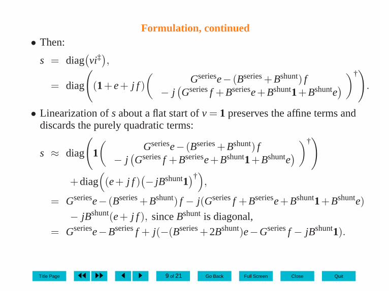
Formulation, continued∙ Then:

s = diag(

vi‡)

,

= diag

(

(1+ e+ j f )

(

Gseriese− (Bseries+Bshunt) f− j(

Gseriesf +Bseriese+Bshunt1+Bshunte)

)†)

.

∙ Linearization ofs about a flat start ofv = 1 preserves the affine terms anddiscards the purely quadratic terms:

s ≈ diag

(

1(

Gseriese− (Bseries+Bshunt) f− j(

Gseriesf +Bseriese+Bshunt1+Bshunte)

)†)

+diag(

(e+ j f )(

− jBshunt1)†)

,

= Gseriese− (Bseries+Bshunt) f − j(Gseriesf +Bseriese+Bshunt1+Bshunte)

− jBshunt(e+ j f ), sinceBshuntis diagonal,

= Gseriese−Bseriesf + j(−(Bseries+2Bshunt)e−Gseriesf − jBshunt1).


Formulation, continued∙ Separatings into real and reactive power injections:

[

pq

]

≈

[

Gseries −Bseries

−(Bseries+2Bshunt) −Gseries

][

ef

]

−

[

0Bshunt1

]

. (1)

∙ Similar form to case in polar coordinates.


3 Special case∙ Purely quadratic terms ins are:

diag(

(e+ j f )(

Gseriese− (Bseries+Bshunt) f − j(

Gseriesf +Bseriese+Bshunte))†)

,

∙ which has real part:

diag(

e(

Gseriese− (Bseries+Bshunt) f)†

+ f(

Gseriesf +Bseriese+Bshunte)†)

,

∙ Following Zhang and Tse [9, Appendix], ife = 0 andGseries= 0 then thereal part of the quadratic term equals zero.

∙ For givenp, if we solvep =−Bseriesf for f thenv = 1+ j f is an exactsolution to the power flow equations.

∙ Corresponding reactive power injections are:

q = diag(

−1(

Gseriesf +Bshunt1)†

− f(

(Bseries+Bshunt) f)†)

,

= −Gseriesf −Bshunt1−diag(

f(



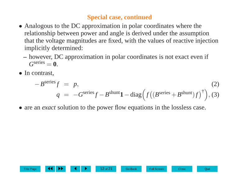
Special case, continued∙ Analogous to the DC approximation in polar coordinates where the

relationship between power and angle is derived under the assumptionthat the voltage magnitudes are fixed, with the values of reactive injectionimplicitly determined:– however, DC approximation in polar coordinates is not exacteven if

Gseries= 0.∙ In contrast,

−Bseriesf = p, (2)

q = −Gseriesf −Bshunt1−diag(

f(


, (3)

∙ are anexact solution to the power flow equations in the lossless case.


4 Numerical example∙ Consider a two bus system with:

– a single line joining the two buses having series admittance1− j10 andno shunt admittance,

– one of the buses having phasor voltage held at 1+ j0∈ ℂ, and– the other bus having phasor voltage 1+ e+ j f ∈ ℂ.

∙ We consider the exact and linearized approximations for thereal andreactive power injected at the other bus as a function of the bus phasorvoltage.

∙ Consider DC approximations in terms of both polar and rectangularcoordinates.


4.1 Real power

00.2

0.40.6

0.81

−1

−0.5

0

0.5

1−10

−5

0

5

10

1+ ef

p

Approximation inpolar coordinates

Approximation in polar coordinates

Exact injectionApproximation in rectangular coordinates

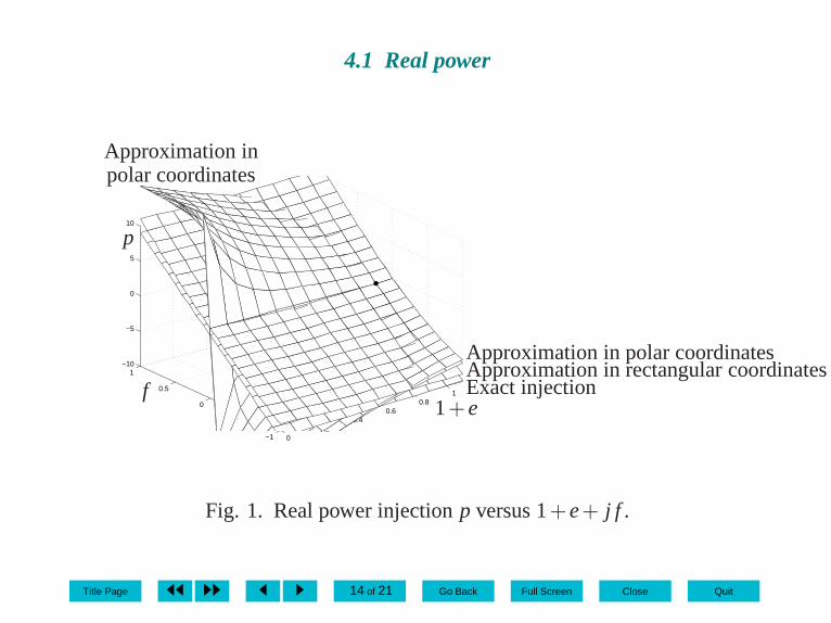
Fig. 1. Real power injectionp versus 1+ e+ j f .


Real power, continued∙ Exact real power injection and the approximation in terms ofrectangular

coordinates are qualitatively close together throughout the graphed range:– approximate sensitivities also close to the actual sensitivities.

∙ DC approximation of real power in terms of polar coordinatesdeviatessignificantly from the exact value for some values of 1+ e+ j f .

∙ In the half-annular region where voltage magnitudes are within 10% of 1per unit:– for small values of voltage phasor angle, smaller thanπ/4 say, and

voltage magnitudes close to one per unit, DC approximation of realpower in polar coordinates is highly accurate.

– for large angles or for voltage magnitudes deviating significantly fromone per unit, the approximation can be quite poor.

∙ Sensitivities of real power injection to changes in the magnitude andangle are relatively far from the actual sensitivities.

∙ Approximation of real power in rectangular coordinates is qualitativelybetter match to actual injection than approximation in polar coordinates.


4.2 Reactive power

00.2

0.40.6

0.81

−1

−0.5

0

0.5

1−10

−5

0

5

10

1+ ef

q

Approximation in polar coordinates

Exact injection

Approximation in rectangular coordinates

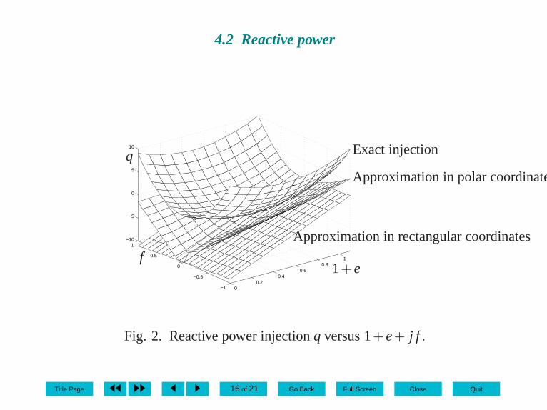
Fig. 2. Reactive power injectionq versus 1+ e+ j f .


Reactive power, continued∙ Approximate reactive power injections in terms of rectangular

coordinates is poorer than the conventional DC approximation in terms ofpolar coordinates.

∙ Functional dependence one and f is highly non-linear.


5 Improved approximation for reactive power∙ Following Coffrin and Van Hentenryck [11], propose piecewise

linearizing reactive power while maintaining the linear approximation ofreal power:

p =[

Gseries −Bseries]

[

ef

]

,

⎡

⎣

q...q

⎤

⎦ ≥

⎡

⎣

−(Bseries+2Bshunt) −Gseries

⋅ ⋅ ⋅ ⋅ ⋅ ⋅

⋅ ⋅ ⋅ ⋅ ⋅ ⋅

⎤

⎦

[

ef

]

−

⎡

⎣

Bshunt1⋅ ⋅ ⋅

⋅ ⋅ ⋅

⎤

⎦ .

∙ where the terms⋅ ⋅ ⋅ would be calculated from linearization about otheroperating points besidesv = 1:– could be calculated off-line.


6 Extensions and conclusions∙ Developed linearization of power flow in rectangular coordinates.∙ Accurate for real power, but not for reactive power.∙ In the lossless case without explicit representation of reactive power,

non-linear power flow can be solved exactly through the solution of alinear equation and substitution to evaluate reactive power injections.

∙ Piecewise linearization may be an effective approach wherereactivepower is to be explicitly represented.

∙ Analogous approximations can be developed for current and complexpower flow as a function of the rectangular representation [3].


References

Allen J. Wood and Bruce F. Wollenberg.Power Generation, Operation, andControl. Wiley, New York, second edition, 1996.

Brian Stott, Jorge Jardim, and Ongun Alsac. DC power flow revisited. IEEETransactons on Power Systems, 24(3):1290–1300, August 2009.

Ross Baldick. Variation of distribution factors with loading. IEEE Transactionson Power Systems, 18(4):1316–1323, November 2003.

Ross Baldick, Udi Helman, Benjamin F. Hobbs, and Richard P. O’Neill. Design


of efficient generation markets.Proceedings of the IEEE,93(11):1998–2012, November 2005.

Thomas J. Overbye, Xu Cheng, and Yan Sun. A comparison of the AC and DCpower flow models for LMP calculations. To appear at HICCS, 2004.

Ross Baldick, Krishnan Dixit, and Thomas Overbye. Empirical analysis of thevariation of distribution factors with loading. InProceedings of the IEEEPower and Energy Society General Meeting, San Francisco, California,June 2005.

G. L. Torres and V. H. Quintana. An interior-point method fornonlinear optimalpower flow using voltage rectangular coordinates.IEEE Transactons onPower Systems, 13(4):1211–1218, November 1998.

J. Lavaei and S. H. Low. Zero duality gap in optimal power flow problem. IEEETransactons on Power Systems, 27(1):92–107, February 2012.

B. Zhang and D. Tse. Geometry of injection regions of power networks. IEEETransactons on Power Systems, 27(2), May 2012.

Javad Lavaei and Steven Low. Zero duality gap in optimal power flow problem.IEEE Transactons on Power Systems, 2012.

Carleton Coffrin and Pascal Van Hentenryck. A linear-programmingapproximation of AC power flows. To appear inIEEE Transactions onPower Systems, 2013.


dc power ﬂow in rectangular coordinates -...

Documents