demand side management: potential and impact on … side management: potential and impact on the...
TRANSCRIPT

eeh power systemslaboratory
Demand Side Management:Potential and impact on the Swiss
transmission grid
Master ThesisPSL1431
Emanuel [email protected]
Power Systems Laboratory
Swiss Federal Institute of Technology (ETH) Zurich
in co-operation with
Swissgrid AG
Supervisors:
Dr. Yee Shan Cherry Yuen, Theodor Borsche
Examiner:
Prof. Dr. Goran Andersson
April 9, 2015

Acknowledgements
First I would like to thank Dr. Cherry Yuen for your dedicated supervision. Withyour great mentoring ability and expertise, you have given me massive supportduring this thesis and aided my personal and professional development.
Further thanks go to Theodor Borsche. With your experience and technicalknowledge, you have excellently enhanced my work, always willing to answer myquestions in explicit detail.
I also want to thank Dr. Arthur Janssen for enabling this Master’s thesisat your department. Carrying out the this thesis within your team was botha valuable professional and an enjoyable personal experience. I thank you andyour team for fully integrating me from the first day.
Additionally, I would like to thank Prof. Dr. Goran Andersson for giving methe chance to write this Master’s thesis in cooperation with your laboratory. Ialso thank you for your competent guidance through the studies at ETH as mytutor.
I furthermore thank Elliott, Manuelz and Helveticus for making the time inZurich so pleasurable.
Ich bedanke mich außerdem bei meiner Familie und Shirin fur eure unendlicheUnterstutzung und Geduld. Ohne euch hatte ich es niemals so weit gebracht.
i

Abstract
In Switzerland activity in Demand Side Management (DSM) is growing on theancillary services markets. New technologies and a changing, more liberalizedmarket environment could trigger DSM activity on a wholesale markets level aswell. This Master’s thesis analyzes how DSM could affect the future Swiss load-profile. A framework is provided, assessing the shiftable power in Switzerlandfor every hour in the years 2020, 2025, 2035 and 2050. Furthermore, possi-ble modifications to the shape of the typical load-profiles in Switzerland due tochanges in technologies and consumption behavior are assessed. Using the de-termined future load-shifting potentials and load-profiles, different optimizationapproaches are followed in order to evaluate possible effects of DSM and storagetechnologies on the hourly Swiss load-profiles in the respective years. The op-timization generally models cost-optimized load-shifting which does not impairend-user functions. Two fundamentally different scenarios for the developmentof the Swiss energy system are considered, one representing a more restraineddevelopment, the other one a very progressive development towards renewables,which includes a swift expansion of Smart-Metering infrastructure as well.
With an hourly shiftable power of up to 2400 MW and a yearly shiftableenergy of up to 12.6 TWh in 2050, Switzerland has very high DSM potential,especially if a progressive path towards renewables is followed. Generally, theshiftable power in winter is around twice the amount in summer due to heatingloads, which qualify well for DSM. In winter, the shiftable power at nighttime ishigher than at daytime, whereas in summer it is predominant at daytime.
If DSM is operated properly, it can lead to essential improvements in theutilization of renewables in the system, allowing for an adaptation of the load-profile to their generation scheme. Higher penetrations of renewables improvethe economic viability of DSM and battery storage, as they allow for the avoid-ance of generation from expensive sources. Therefore, in the progressive scenariotowards renewables an increasing trend in the possible savings is observed, induc-ing possible yearly savings of more than 150 million Swiss Francs through DSMand battery storage in 2050. For residential end-users, DSM can this way be-come profitable in 2035, if the households include an electric vehicle. Industrialand commercial consumers can profit earlier. However, a decreasing tendencyof the actually used fraction of the shiftable load can also be determined: Themore DSM and battery storage is present in the system, the less is actuallyused, proportionally. This implies a declining trend in the possible savings andan advantage for early adopters of DSM. In a progressive development towardsrenewables, this declining trend is outweighed by the growing possible savings
ii

iii
due to better utilization of renewables. On the contrary, in a scenario with arestrained introduction of renewables the declining trend is predominant. HereDSM only allows for very low savings. For residential end-users, neither DSM norbattery storage are profitable in this scenario. However, industrial and commer-cial consumers could achieve cost-effective DSM-systems, in spite of the decliningtrend in savings.
Independent, price-driven load-shifting can provoke undesirable effects on theload-profile. Uncontrolled real-time or time-of-use pricing structures can lead tovery sharp load-peaks in times of low prices, which can cause problems to thesystem operators. Altogether, the way DSM is incentivized and controlled iscrucial for the resulting effect on the load-profile.
Over the course of this thesis, the projected DSM-potentials for the differentyears and scenarios are embedded in a DSM simulation tool, which is imple-mented for Swissgrid AG. This tool enables the simulation of possible effects ofDSM on the Swiss load-profile, based on variable input data. It is to be usedwithin the transmission system planning framework of Swissgrid AG.
Keywords: Demand Side Management, load-shifting, electric vehicles, electricenergy storage

Contents
Acknowledgements i
Abstract iii
Acronyms vi
1 Introduction 1
1.1 Change in power systems . . . . . . . . . . . . . . . . . . . . . . 2
1.2 Contribution of this thesis . . . . . . . . . . . . . . . . . . . . . . 5
2 Assessment of load-shifting potentials in Switzerland 7
2.1 Residential sector . . . . . . . . . . . . . . . . . . . . . . . . . . . 9
2.2 Industrial and services sector . . . . . . . . . . . . . . . . . . . . 22
2.3 Transport sector . . . . . . . . . . . . . . . . . . . . . . . . . . . 32
2.4 Pure load-shifting technologies . . . . . . . . . . . . . . . . . . . 40
3 Optimization approaches 46
3.1 Underlying data . . . . . . . . . . . . . . . . . . . . . . . . . . . 48
3.2 Effect of new technologies and changes in consumption on initialSwiss load-profiles . . . . . . . . . . . . . . . . . . . . . . . . . . 51
3.2.1 Data . . . . . . . . . . . . . . . . . . . . . . . . . . . . . . 51
3.2.2 Calculation of new load-profiles . . . . . . . . . . . . . . . 54
3.3 Optimization basis . . . . . . . . . . . . . . . . . . . . . . . . . . 55
3.4 Market cost minimization approach . . . . . . . . . . . . . . . . . 58
3.5 Load-dependent tariffs approach . . . . . . . . . . . . . . . . . . 61
3.6 Day- and night-tariffs approach . . . . . . . . . . . . . . . . . . . 62
3.7 Real-time pricing approach . . . . . . . . . . . . . . . . . . . . . 63
3.8 Real-time pricing combined with load-dependent tariffs approach 65
iv

Contents v
4 Results and Discussion 66
4.1 Assessment of load-shifting potentials . . . . . . . . . . . . . . . 67
4.2 Effect of new technologies and changes in consumption on initialSwiss load-profiles . . . . . . . . . . . . . . . . . . . . . . . . . . 73
4.3 Market cost minimization approach . . . . . . . . . . . . . . . . . 74
4.4 Load-dependent tariffs approach . . . . . . . . . . . . . . . . . . 77
4.5 Day- and night-tariffs approach . . . . . . . . . . . . . . . . . . . 79
4.6 Real-time pricing approach . . . . . . . . . . . . . . . . . . . . . 81
4.7 Real-time pricing combined with load-dependent tariffs approach 83
4.8 Battery and CAES-storage . . . . . . . . . . . . . . . . . . . . . 84
4.9 Possible savings for end-users . . . . . . . . . . . . . . . . . . . . 88
5 Conclusion and Outlook 94
5.1 Limits . . . . . . . . . . . . . . . . . . . . . . . . . . . . . . . . . 99
A Appendix A-1
A.1 Effect of new technologies and changes in consumption on initialSwiss load-profiles . . . . . . . . . . . . . . . . . . . . . . . . . . A-1
A.2 Market cost minimization approach . . . . . . . . . . . . . . . . . A-10
A.3 Load-dependent tariffs approach . . . . . . . . . . . . . . . . . . A-20
A.4 Day- and night-tariffs approach . . . . . . . . . . . . . . . . . . . A-30
A.5 Real-time pricing approach . . . . . . . . . . . . . . . . . . . . . A-40
A.6 Real-time pricing combined with load-dependent tariffs approach A-50

Acronyms
EU European Union
DSM Demand Side Management
AC air conditioning
CAES Compressed Air Energy Storage
VSE Verband Schweizerischer Elektrizitatsunternehmen
BFE Bundesamt fur Energie (Swiss Federal Office of Energy)
TSO Transmission System Operator
DSO Distribution System Operator
WWB weiter wie bisher (”business as usual”)
NEP neue Energiepolitik (”new energy policy”)
AMM Automated Meter Management
AMR Automated Meter Reading
NTC Net Transfer Capacity
VPP virtual power plant
RTP real-time pricing
TOU time-of-use
vi

Chapter 1
Introduction
1

1. Introduction 2
1.1 Change in power systems
With the vast increase in renewable electricity generation in Europe, a highamount of inflexible electricity generation has been introduced into the electricitymarkets. The inflexibility, prediction-uncertainty and the partially decentralizedapproach of renewables imply new challenges to energy and power system utilities(VSGS, 2013). Meanwhile, the federal council of Switzerland decided the step-wise nuclear power phase-out in 2011; the last Swiss nuclear power plant will beshut down in 2034. It is intended to replace the nuclear base load, which after allsupplies around 40 % of the current Swiss electricity consumption, mainly withgeneration from hydro and renewables. However, in order to ensure grid stabil-ity, electricity supply and demand have to always remain in balance. For theintegration of the hence more and more increasing amount of inflexible and par-tially decentralized generation, the Bundesamt fur Energie (Swiss Federal Officeof Energy) (BFE) suggests a development towards a Smart-Grid. The Smart-Grid ”enables the direct interaction between customers, grid and generators andholds high optimization potential for the power system”. BFE (2011)
In this thesis, we focus on the flexibilization of the electricity demand-side,which is commonly referred to as Demand Side Management (DSM). Historically,the electricity demand-side has been very inelastic. The basic idea of DSM is tomake the loads flexible, in order to allow them to react to different power systemor market situations.
DSM generally has to find the balance between two objectives that are oftencompeting: First, DSM aims to influence the load in order to achieve a desiredpower consumption at a given time. Second, the end-user function should bemaintained and not impaired. (Callaway & Hiskens, 2011).
According to de Haan et al. (2012), there are three different approachesof DSM. First, shifting loads with thermal storage, e.g. electric water boilers,which can ideally be carried out without impacting consumption patterns. Theshifting can be accomplished by either ”filling the thermal reservoir” beforehand,or regenerating it afterwards (Berner et al., 2014). Second, shifting the time of anenergy service, e.g. washing the laundry at a different time. And third, switchingloads on and off directly, i.e. the abandonment of an energy service, which alsoapplies for electricity storage devices such as batteries or compressed air energystorage.
Load shifting can be either be triggered by price-signals, motivating end-usersto shift their electricity consumption to times with low electricity prices, or bycentralized control strategies. The latter is executed by the system operator andusually needs an aggregator at the interface between load and system operator.Price signals can either be realized by offering the end-users time-varying tariffsand allowing them to shift their electricity independently, or by introducingaggregated DSM to electricity wholesale markets.

1. Introduction 3
Today, ripple control is already in use for switching the majority of elec-tric heaters, heat pumps and water boilers. The switching of the electric metersbetween day- and night tariffs is done via ripple control as well, which, in Switzer-land, is executed by the Distribution System Operator (DSO). (Baeriswyl et al.,2012) Therefore, a centrally operated DSM is already present in Switzerland.
Time varying electricity-tariffs have already been deployed almost all overSwitzerland. They consist of a day-tariff, between 6 a.m. and 10 p.m. and anight-tariff between 10 p.m. and 6 a.m., whereat the day-tariff is usually 50 % to100 % higher than the night-tariff. (EKZ, 2013)
In order to take advantage of price-signals more flexibly, end-users need to beconnected to a Smart-Meter. The most basic Smart-Meter-function is to trackthe customer’s electricity consumption with a time-stamp and send it to theprovider. This function is commonly referred to as Automated Meter Reading(AMR) and enables time-coupled electricity tariffs, so called time-of-use (TOU)-pricing. TOU-pricing provides different prices throughout the day, which areusually fixed well in advance. The day- and night tariff model in Switzerland isa simple version of TOU-pricing.
More advanced Smart-Meters are available, which allow for Automated Me-ter Management (AMM). These Smart-Meters are able to communicate withcentralized systems on short time-scales, switch dynamically between electricitytariffs and turn specific loads on and off. (Baeriswyl et al., 2012) They per-mit controlled load-shifting strategies and much more advanced pricing models,such as real-time pricing (RTP). RTP aims to provide the end-users with aprice, reflecting the utilities’ generation cost, e.g. by charging them the real-timespot-market price.
In 2012, the BFE has commissioned a study on the impact assessment ofSmart-Meters in Switzerland. This study yielded that an area-wide introductionof Smart-Meters is generally profitable. However, ”the large corresponding load-shifting potential only leads to small benefit, while the relatively small potentialefficiency improvement holds great benefit.” (Baeriswyl et al., 2012). Many Swissenergy utilities already started to distribute Smart-Meters to some of their cus-tomers, yet mainly for research and testing purposes. Furthermore, several DSMand Smart-Grid pilot projects were launched. In the following, we give someexamples of current projects in Switzerland.
On the Swiss ancillary services markets, Growing activity in DSM could beobserved lately. The pilot project FlexLast, launched by BKW, IBM, Migrosand Swissgrid, assessed the feasibility of generating secondary control energywith shiftable industrial loads. They concluded that ”the generation of controlenergy with industrial load is generally possible. The entry barriers for secondarycontrol reserves are high [...] but could be overcome by pooling industrial loads.”In 2015, the Swisscom Energy Solutions AG successfully placed their ”smartstorage network” tiko on the ancillary services market. They use the aggregated
1. Introduction 4
power of residential heating systems as a virtual power plant (VPP), in order toprovide control reserve power. (Swisscom, 2015).
EKZ has decided the full Smart-Meter rollout in 2013 (EKZ, 2013). Theyplan to equip all their customers with Smart-Meters within the ”next 15 to20 years”. However, the Smart-Meters installed by EKZ provide only AMR-functions. Thus, they cannot manage loads independently and do not enableRTP. BKW is active in the Smart-Metering and DSM field as well. Within theirpilot project Inergie iSMART, they aim to intelligently integrate decentralizedgeneration into their distribution grids. So far, they have equipped customers anddecentralized photovoltaic systems with Smart-Meters in order to collect relevantdata. (BKW, 2015). Moreover, CKW, a member of the Axpo group, launched aSmart-Metering pilot-project in 2010. In 2011, they introduced different pricingmodels. The customers can choose between TOU-pricing, consisting of fourdifferent tariffs throughout the day, and an RTP-model, which is based on thecurrent market situation. (CKW, 2011)
With GridSense, developed by Alpiq, an intelligent consumption optimiza-tion technology is already in the Swiss market. The technology can control theuse of charging stations for electric vehicles, hot-water boilers, heat-pumps, bat-teries and photovoltaic systems. The goal is to optimize the respective user’sdemand according to the current power system situation. This should improvethe utilization of renewables and increase the end-users’ self-sufficiency, whilereducing the needed expenses for grid-upgrades on the supplier-side. The tech-nology can operate decentrally, but can also communicate with utilities, in orderto enter ancillary-services markets. Morf (2014)
Therefore, many new projects that are relevant for DSM were launched inSwitzerland, lately. The full market opening, which is planned for 2018 mightfurther enhance this trend.
The Smart-Grid approach takes the idea of customer participation a step fur-ther. According to VSGS (2013), the term Smart-Grid describes a power systemthat intelligently controls the whole power-system infrastructure, in order to per-mit its optimum and most efficient operation in any situation. This way, moreintelligence in the power system can avoid expensive grid-upgrades. The Swissassociation for Smart-Grids (VSGS), founded in 2011, concentrates the activityof 13 large Swiss electricity-utilities, with the goal to ”promote the introductionof a Smart-Grid in Switzerland” (VSGS, 2013). Furthermore, extensive Smart-Grid research activity has been undertaken by large technology groups such asABB, Siemens or GE recently. In this context, DSM can be seen as one part ofan evolution towards Smart-Grids.

1. Introduction 5
1.2 Contribution of this thesis
This thesis addresses two main questions:
1. Which individual technologies qualify for DSM, what is their potential andhow will they develop in future?
2. How can these technologies be modeled and how can they affect the futureSwiss load-profile?
In order to answer these questions, we derive hourly profiles of the shiftablepower for relevant load-categories in the residential, industrial and services andtransport sector in Switzerland. Furthermore, the effects of new technologiesand changes in consumption behavior on the shape of typical future load-profilesare assessed. We then model the possible impact of a cost optimizing operationof DSM on the Swiss load-profile, based on the determined shiftable-power andfuture load-profiles. Using five different modeling approaches, we simulate theeffect of different strategies to control or incentivize DSM. The analysis aims tomodel possible effects of DSM that are relevant for load and generation scheduleson an hourly basis. Load-shifting activity on ancillary-services markets is notconsidered, as ancillary services are used to compensate for real-time imbalancesand do not affect the preceding scheduling. This work is carried out in cooper-ation with Swissgrid AG, the Swiss Transmission System Operator (TSO). Themain goal of the thesis is to develop a tool to simulate possible future effects ofDSM, based on various input data. The tool is to be used in their power systemplanning process.
The analysis is aligned with the Swiss energy-outlook for 2050 (Kirchneret al., 2012), published by the BFE in 2012. The energy-outlook contains dif-ferent scenarios for the development of the Swiss energy system, which form avery important source for transmission system planning in Switzerland. In thisthesis, DSM is analyzed for the relevant years 2020, 2025, 2035 and 2050. Thedata basis of the analysis is provided by the scenarios weiter wie bisher (”busi-ness as usual”) (WWB) and neue Energiepolitik (”new energy policy”) (NEP)of the energy-outlook. The WWB-scenario projects a restrained developmentof the energy system, partially introducing fossil fuel based electricity genera-tion, whereas the NEP-scenario projects a very progressive development towardsrenewables.
A related analysis for the residential sector in Switzerland has been performedby de Haan et al. (2012). They provide own scenarios for the development of theSwiss energy system to estimate corresponding shifting potentials of residentialloads. However, their scenarios differ from the Swiss energy-outlook (Kirchneret al., 2012), with which the estimations presented in this thesis are much morealigned. Nevertheless, we use de Haan et al. (2012) as an important source and

1. Introduction 6
Scenario yearYearly shiftable energy per duration≤ 15 min ≤ 1 h ≤ 2 h ≤ 4 h > 4 h
Restrained2020 10.1 9.6 9.2 5.8 2.42035 10.0 9.6 9.1 5.7 2.42050 9.9 9.4 9.0 5.7 2.4
Progressive2020 9.5 9.0 8.6 5.3 2.22035 7.0 6.5 6.1 3.6 1.52050 4.8 4.3 3.9 2.1 0.7
Table 1.1: The table shows the potential yearly shiftable energy in the residentialsector from de Haan et al. (2012) in TWh.
reference point for comparing our results. Table 1.1 lists their results for theyearly shiftable electric energy in the residential sector. As the table shows,they found a yearly shiftable energy ranging between 2.2 and 9.6 TWh, whichtranslates to 7.9 to 34.5 PJ.
We furthermore use the study on the potential of Smart Meters in Switzerlandby Baeriswyl et al. (2012) as one of our main references. They have assessed load-shifting potentials in the residential and the industrial and services sector, as wellas for electric vehicles. Their analysis was based on the 2009 version of the Swissenergy-outlook 2050, published by BFE. For the year 2035 in their conservativescenario, they found combined load-shifting potentials with a duration of shiftingof 1 hour of up to 299 MW, of which 236 MW can also be shifted for 2 hours and184 MW for 4 hours. The respective numbers for their progressive scenario are1382 MW for 1 hour, 1090 MW for 2 hours and 840 MW for 4 hours. However,these numbers do not include the already used shifting potential of hot-waterand space-heating loads.

Chapter 2
Assessment of load-shiftingpotentials in Switzerland
7

2. Assessment of load-shifting potentials in Switzerland 8
In this chapter, technologies that potentially qualify for load-shifting areanalyzed. They are categorized according to their respective economic sector,i.e. residential, industrial and services and transport sector. This categorizationis chosen due to similar approaches in relevant literature, especially in the stud-ies by Kemmler et al. (2014) and Baeriswyl et al. (2012), published by BFE.Furthermore, there are substantial differences between the three different sectorsin terms of load-size (energy and power) and operating hours. This could lead todifferent exploitation-, incentive- and control-strategies of the loads in the threesectors.
In the last section of this chapter we analyze the potential of technologieswith the sole purpose of load-shifting, i.e. they do not have another purpose asfor example electric heat pumps, which are mainly installed for space heating.
Our analysis of DSM potentials follows a top-down approach, starting withdata of the yearly energy-consumption per technology from Kemmler et al. (2014)and Kirchner et al. (2012). We then assess typical seasonal and daily consump-tion patterns in order to estimate the hourly DSM-potentials from the yearlyconsumption.
The load-shifting potential always depends on the desired duration of action.If, for instance, one wants to store electric energy as heat, the time by whichthe heat-load can be turned on in advance is limited, due to the occurring heatloss. Therefore, not only the shiftable power and energy, but also the possibleduration of shifting per technology is assessed in this study.
In addition to the potential shiftable power and energy, the technological ex-ploitation of the respective loads is important, in order to carry out load-shifting.Load-shifting based on TOU-pricing needs the functionality of the AMR Smart-Meters. Centralized load-shifting and RTP require AMM-Smart-Meters. Themarket-exploitation of load-shifting is hence limited by the distribution of Smart-Meters, which is commonly referred to as their rollout-factor. Baeriswyl et al.(2012) present different scenarios for the Smart-Meter rollout. As our analysisis based on the projections of the Swiss energy-outlook 2050 by Kirchner et al.(2012), we correlate the rollout factors from Baeriswyl et al. (2012) to scenariosfrom the energy-outlook. Therefore, the selective rollout-scenario by Baeriswylet al. (2012) is correlated with the WWB scenario in the energy-outlook, whilethe progressive rollout-scenario is correlated with the NEP scenario. Table 2.1contains the respective Smart-Meter rollout-factors, extrapolated from Baeriswylet al. (2012).
Most of our succeeding optimization approaches require Smart-Meters withAMM-functionalities. The rollout factors in Table 2.1 thus refer to Smart-Meterswhich qualify for AMM.

2. Assessment of load-shifting potentials in Switzerland 9
Scenario 2020 2025 2035 2050
Smart-Meter rolloutWWB 8 % 12 % 20 % 35 %NEP 40 % 80 % 90 % 95 %
Table 2.1: The table shows the percentage Smart-Meter distribution (rollout-factors), extrapolated from Baeriswyl et al. (2012).
2.1 Residential sector
Table 2.2 gives an overview over the development of the electricity use in theresidential sector, broken down into individual load-categories. The historicalvalues arise from Kemmler et al. (2014). The forecast values are obtained fromKirchner et al. (2012), which contains different scenarios for the developmentof the Swiss energy-system. The values in the table arise from their scenariosWWB and NEP and give a range for the expected future loads. Since Kirchneret al. (2012) does not contain values for the year 2025, the corresponding tableentries are calculated as the arithmetic mean of the years 2020 and 2030. Thetable indicates the largest residential energy consumption by appliances andprocesses, space heating and hot water.
Application 2000 20132020 2025 2035 2050
WWB NEP WWB NEP WWB NEP WWB NEP
Space heating 12.2 15.7 15.0 14.6 14.4 13.1 13.0 9.9 10.8 6.2of which el. HP 1.5 5.0 6.4 6.8 7.1 7.2 7.9 7.2 7.7 4.8
Hot water 8.3 8.6 8.6 8.9 8.3 8.5 7.8 7.3 6.9 2.9of which el. HP 0.2 0.6 1.0 1.1 1.3 1.5 1.6 2.0 1.9 2.6
Cooking stoves 4.8 4.9 5.4 5.3 5.5 5.3 5.5 5.3 5.5 4.8
Lighting 5.7 5.0 3.1 3.0 2.8 2.4 2.0 1.4 1.3 0.9
Ventilation,3.6 4.6 5.2 5.0 5.8 5.3 7.0 6.0 10.4 8.3AC, building-
services
IC & consumer5.4 4.9 5.2 5.1 5.3 5.1 5.3 4.8 5.2 4.5
electronics
Appliances &12.9 15.8 14.1 13.9 13.9 13.3 13.6 12.3 13.5 11.2
processes
Other devices 4.4 7.8 8.1 7.9 8.7 8.4 9.6 9.1 10.5 9.7
Sum 57.3 67.2 64.6 63.9 64.3 61.3 63.8 55.9 64.1 48.8
Table 2.2: The table shows the electricity use of residential loads in Switzerlandin PJ from Kemmler et al. (2014) and Kirchner et al. (2012).
According to de Haan et al. (2012), cooking stoves, lighting and information,communication and consumer electronics do not qualify for DSM. Those tech-

2. Assessment of load-shifting potentials in Switzerland 10
ApplicationShifting potential per duration
≤ 15 min ≤ 1 h ≤ 2 h ≤ 4 h > 4 h
Space heating 100 % 100 % 100 % 50 % 5 %
Hot water 100 % 100 % 100 % 95 % 60 %
Ventilation,100 %* 0 %* 0 %* 0 %* 0 %*
air conditioning
Refrigerators 100 % 100 % 100 % 50 % 5 %
Freezers 100 % 100 % 100 % 100 % 100 %
Washing machines,15 % 10 % 5 % 0 % 0 %dryers and
dishwashers
Table 2.3: The table shows the percentage shifting potential of residential loadsper duration. The values originate in the report by de Haan et al. (2012). Thevalues marked with * derive from Baeriswyl et al. (2012).
Application Winter Spring and fall Summer
Space heating 60 % 40 % 0 %
Hot water 25 % 50 % 25 %
Ventilation, air conditioning15 % 50 % 35 %
and building services
Appliances and processes 25 % 50 % 25 %
Table 2.4: The table shows the percentage seasonal allocation of residentialelectricity consumption, estimated from de Haan et al. (2012).
nologies do not allow for energy storage and their consumption patterns are veryinflexible. Moreover, the category other devices is omitted in this analysis, sincethe devices are not specified and hence cannot be assessed. We therefore focuson the remaining load-categories listed in Table 2.2. These are space heating,hot water, ventilation, air conditioning and building services and appliances andprocesses.
For the estimation of the DSM-potential, we need the following data, obtainedfrom de Haan et al. (2012): The percentage shifting potential of residential loadsper duration, which is listed in Table 2.3 and the in Table 2.4 shown percentageseasonal allocation of the consumption per technology. The data in the lattertable have been estimated from de Haan et al. (2012) under certain assumptions;first, we assume four equally long seasons throughout the year and second weassume that no space heating occurs during the three summer months. We fur-thermore use the daily residential load profiles from de Haan et al. (2012) as areference point to create our own daily load profiles per technology.
2. Assessment of load-shifting potentials in Switzerland 11
Space heating
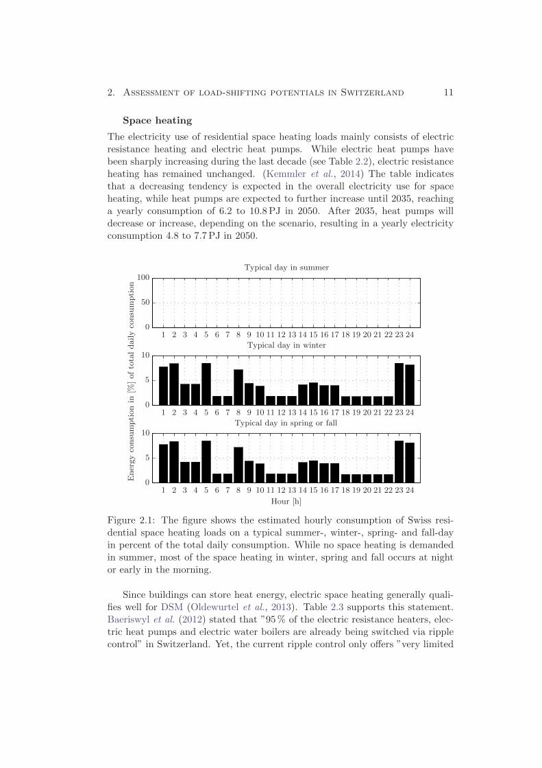
The electricity use of residential space heating loads mainly consists of electricresistance heating and electric heat pumps. While electric heat pumps havebeen sharply increasing during the last decade (see Table 2.2), electric resistanceheating has remained unchanged. (Kemmler et al., 2014) The table indicatesthat a decreasing tendency is expected in the overall electricity use for spaceheating, while heat pumps are expected to further increase until 2035, reachinga yearly consumption of 6.2 to 10.8 PJ in 2050. After 2035, heat pumps willdecrease or increase, depending on the scenario, resulting in a yearly electricityconsumption 4.8 to 7.7 PJ in 2050.
Typical day in spring or fall
Hour [h]
Typical day in winter
Energyconsumptionin
[%]oftotaldailyconsumption
Typical day in summer
1 2 3 4 5 6 7 8 9 10 11 12 13 14 15 16 17 18 19 20 21 22 23 24
1 2 3 4 5 6 7 8 9 10 11 12 13 14 15 16 17 18 19 20 21 22 23 24
1 2 3 4 5 6 7 8 9 10 11 12 13 14 15 16 17 18 19 20 21 22 23 24
0
5
10
0
5
10
0
50
100
Figure 2.1: The figure shows the estimated hourly consumption of Swiss resi-dential space heating loads on a typical summer-, winter-, spring- and fall-dayin percent of the total daily consumption. While no space heating is demandedin summer, most of the space heating in winter, spring and fall occurs at nightor early in the morning.
Since buildings can store heat energy, electric space heating generally quali-fies well for DSM (Oldewurtel et al., 2013). Table 2.3 supports this statement.Baeriswyl et al. (2012) stated that ”95 % of the electric resistance heaters, elec-tric heat pumps and electric water boilers are already being switched via ripplecontrol” in Switzerland. Yet, the current ripple control only offers ”very limited

2. Assessment of load-shifting potentials in Switzerland 12
flexibility”. In contrast, BKW, one of the large Swiss energy suppliers introducedflexible switching of loads via ripple control in 2014 (BKW AG, 2014).
In this analysis, we assume that electric heaters and electric heat pumps donot differ in their load shifting behavior.
Typical day in spring or fall
Hour [h]
Typical day in winter
Energyconsumptionin
[%]oftotaldailyconsumption
Typical day in summer
1 2 3 4 5 6 7 8 9 10 11 12 13 14 15 16 17 18 19 20 21 22 23 24
1 2 3 4 5 6 7 8 9 10 11 12 13 14 15 16 17 18 19 20 21 22 23 24
1 2 3 4 5 6 7 8 9 10 11 12 13 14 15 16 17 18 19 20 21 22 23 24
0
20
40
0
20
40
0
20
40
Figure 2.2: The figure shows the estimated hourly electricity consumption ofSwiss residential hot water loads on a typical summer-, winter-, spring- and fall-day in percent of the total daily consumption. In all seasons, the bulk electricityuse occurs at night, which is a result of the ripple control.
In order to identify the shiftable load of space heating, we extract the typicalload profiles of space heating appliances from de Haan et al. (2012). Since theyonly provide load-profiles for typical summer- and winter-days, for spring andfall the arithmetic mean is used. Figure 2.1 shows the resulting typical dailyload-profiles of space heating appliances. The summer-profile is zero, while thewinter-, spring- and fall-profiles show a bulk consumption at night and a peakearly in the morning. Since many of the electric resistance heaters and electricheat pumps are already controlled via ripple control, the profile in Figure 2.1contains some shifted load. However, the fraction of space heating loads, whichis already controlled, cannot be identified. Zimmermann et al. (2012) performedan extensive study on the electricity consumption of 251 English households.They found that the bulk-consumption of uncontrolled electric heating in Eng-

2. Assessment of load-shifting potentials in Switzerland 13
land occurs at night and early in the morning as well. Therefore we use theprofile in Figure 2.1 as a representation of the uncontrolled space heating profile.
Hot water
According to Kemmler et al. (2014), the main electric hot water devices arewater boilers and heat pumps. Table 2.2 indicates an increase in hot waterelectricity use until 2020, followed by a decrease until 2050, which leads to ayearly consumption between 2.9 and 6.9 PJ in 2050. However, according to thetable, the electricity use of electric heat pumps will grow steadily until 2050,reaching 1.9 to 2.6 PJ per year.
Similar to space heating appliances, electric hot water devices qualify wellfor load-shifting, due to the high thermal inertia of water (Oldewurtel et al.,2013). Table 2.3 indicates a very high shifting potential per duration of hotwater devices. As previously stated, 95 % of the Swiss electric hot water devicesare already controlled via ripple control.
Typical day in spring or fall
Hour [h]
Typical day in winter
Energyconsumptionin
[%]oftotaldailyconsumption
Typical day in summer
1 2 3 4 5 6 7 8 9 10 11 12 13 14 15 16 17 18 19 20 21 22 23 24
1 2 3 4 5 6 7 8 9 10 11 12 13 14 15 16 17 18 19 20 21 22 23 24
1 2 3 4 5 6 7 8 9 10 11 12 13 14 15 16 17 18 19 20 21 22 23 24
0
10
20
0
10
20
0
10
20
Figure 2.3: The figure shows the hourly consumption of residential hot waterloads from Jordan & Vajen (2001) on a typical summer-, winter-, spring- andfall-day in percent of the total daily consumption. The electricity use peaks inthe morning and in the evening. The profile does not vary seasonally.

2. Assessment of load-shifting potentials in Switzerland 14
Typical day in spring or fall
Hour [h]
Typical day in winter
Energyconsumptionin
[%]oftotaldailyconsumption
Typical day in summer
1 2 3 4 5 6 7 8 9 10 11 12 13 14 15 16 17 18 19 20 21 22 23 24
1 2 3 4 5 6 7 8 9 10 11 12 13 14 15 16 17 18 19 20 21 22 23 24
1 2 3 4 5 6 7 8 9 10 11 12 13 14 15 16 17 18 19 20 21 22 23 24
0
10
20
0
10
20
0
10
20
Figure 2.4: The figure shows the estimated hourly consumption of Swiss residen-tial ventilation, air conditioning and building service-loads on a typical summer-,winter-, spring- and fall-day in percent of the total daily consumption. All elec-tricity use appears during daytime or in the evening.
Using de Haan et al. (2012), we define typical daily load profiles of hot waterelectricity use in Switzerland. This is done the same way as for space heatingdevices. The resulting daily patterns are depicted in Figure 2.2 and show a con-centration of consumption during nighttime and almost no consumption duringdaytime. This profile represents the already controlled demand. However, forthis study, the actual hot-water consumption is more interesting, as we want toexamine the effect of a more flexible control of hot water loads. Therefore, arepresentative load profile of European domestic hot water loads is drawn fromJordan & Vajen (2001). The profile is shown in Figure 2.3, which indicates hotwater load peaks in the morning and in the evening. We consider this profileto be the actual profile of requested hot water and use it for the further analysis.
Ventilation, air conditioning and building services
Among the three appliances in this category, only ventilation and air conditioningqualify for load-shifting. Other buildings services (e.g. elevators, water pumps)are considered to be inflexible. (de Haan et al., 2012). According to Table 2.2, a

2. Assessment of load-shifting potentials in Switzerland 15
Application Winter Spring and Fall Summer
Ventilation, air conditioning15 % 50 % 35 %
and building services
of which building services 15 % 30 % 15 %
of which ventilation0 % 20 % 20 %
and air conditioning
Table 2.5: The table shows the percentage seasonal allocation of electric venti-lation, air conditioning and building services loads, estimated from Table 2.4.
Application 2000 20132020 2025 2035 2050
WWB NEP WWB NEP WWB NEP WWB NEP
Ventilation and1.4 1.8 2.1 2.0 2.3 2.1 2.8 2.4 4.2 3.3
air conditioning
Table 2.6: The table shows the electricity use of residential ventilation and airconditioning loads in Switzerland in PJ. The values are estimated using Kemmleret al. (2014) and Kirchner et al. (2012).
Application 2000 20132020 2025 2035 2050
WWB NEP WWB NEP WWB NEP WWB NEP
Refrigerators 3.5 4.3 3.8 3.8 3.8 3.6 3.7 3.4 3.7 3.1
Freezers 1.9 2.3 2.1 2.0 2.0 2.0 2.0 1.8 2.0 1.6
Dishwashers, wa-5.8 7.1 6.3 6.3 6.3 6.0 6.1 5.5 6.1 5.0shing machines
and dryers
Table 2.7: The table shows the yearly electricity use of residential refrigerators,freezers and dishwashers, washing machines and dryers in Switzerland in PJ. Thevalues are estimated using Kemmler et al. (2014) and Kirchner et al. (2012).
steady increase in the electricity use of ventilation, air conditioning and buildingservices is expected until 2050, resulting in a high yearly electricity consumptionbetween 8.3 and 10.4 PJ in 2050.
Table 2.3 indicates a high load-shifting potential of ventilation and air con-ditioning loads in the first 15 minutes, which vanishes after one hour.
In order to extract the electricity use of ventilation and air conditioning fromthe values listed in Table 2.2, we assume that ventilation and air conditioningonly occurs in summer, spring and fall, while the electricity use of buildingservices does not change seasonally. Using Table 2.4, this assumption leads tothe fragmented seasonal allocation of ventilation, air conditioning and buildingservices as listed in Table 2.5. From these values, we can allocate 40 % of the

2. Assessment of load-shifting potentials in Switzerland 16
Typical day in spring or fall
Hour [h]
Typical day in winter
Energyconsumptionin
[%]oftotaldailyconsumption
Typical day in summer
1 2 3 4 5 6 7 8 9 10 11 12 13 14 15 16 17 18 19 20 21 22 23 24
1 2 3 4 5 6 7 8 9 10 11 12 13 14 15 16 17 18 19 20 21 22 23 24
1 2 3 4 5 6 7 8 9 10 11 12 13 14 15 16 17 18 19 20 21 22 23 24
0
5
0
5
0
5
Figure 2.5: The figure shows the estimated hourly consumption of Swiss residen-tial cooling and freezing loads on a typical summer-, winter-, spring- and fall-dayin percent of the total daily consumption.
yearly electricity consumption in this category to ventilation and air conditioning.The other 60 % are consumed by other building services. Assigning 40 % of theyearly consumption in this category to ventilation and air conditioning yieldsthe values listed in Table 2.6. However, this is only an approximation and theallocation could change in future, if e.g. the residential use of air conditioningexpands disproportionately.
We further assume that the daily percentage load profiles of ventilation andair conditioning in summer, spring and fall are consistent with the respectiveprofiles of building services, i.e. the profiles for summer, spring and fall in Figure2.4 are valid for ventilation and air conditioning. These load profiles are againestimated from de Haan et al. (2012) and show a concentrated consumption atdaytime with peaks in the morning. In summer, a second peak occurs in theevening hours. According to Table 2.5, no electricity consumption from ventila-tion and air conditioning is assumed in winter.
Appliances and processes
This category mainly consists of freezers and refrigerators, dishwashers, wash-

2. Assessment of load-shifting potentials in Switzerland 17
Typical day in spring or fall
Hour [h]
Typical day in winter
Energyconsumptionin
[%]oftotaldailyconsumption
Typical day in summer
1 2 3 4 5 6 7 8 9 10 11 12 13 14 15 16 17 18 19 20 21 22 23 24
1 2 3 4 5 6 7 8 9 10 11 12 13 14 15 16 17 18 19 20 21 22 23 24
1 2 3 4 5 6 7 8 9 10 11 12 13 14 15 16 17 18 19 20 21 22 23 24
0
5
10
0
5
10
0
5
10
Figure 2.6: The figure shows the estimated hourly consumption of Swiss resi-dential washing machines, dryers and dishwashers on a typical summer-, winter-,spring- and fall-day in percent of the total daily consumption.
ing machines, dryers and electrical kitchen devices (e.g. kitchen extractor fans,coffee-machines, toasters, etc.) (Kemmler et al., 2014). Table 2.2 shows a de-creasing tendency of the yearly consumption in this category, which howeverremains large with 11.2 to 13.5 PJ in 2050.
Due to very different daily consumptions patterns (see Figures 2.5 and 2.6)and possible durations of load-shifting (see Table 2.3), this load-category aredivided into the three following subcategories: First, freezers and refrigerators,i.e. energy storing appliances with theoretically high flexibility due to their ther-mal inertia; second, dishwashers, washing machines and dryers with limited flex-ibility and third, electrical kitchen devices, which are considered to be inflexibleand hence not further assessed here. (de Haan et al., 2012) Kemmler et al.(2014) indicates that in 2013, 45 % of the total yearly consumption in this cat-egory were used by dishwashers, washing machines and dryers and 42 % wereconsumed by refrigerators and freezers. We assume that of the latter category,65 % were consumed by refrigerators and 35 % by freezers. Further assumingthe same allocation for the other years, we receive the yearly consumption persubcategory listed in Table 2.7.

2. Assessment of load-shifting potentials in Switzerland 18
Hour [h]
Typical day in spring or fall, year 2020
Shiftable
pow
er[M
W]
Typical day in winter, year 2020
> 4 h≤ 4 h≤ 2 h1 h15 min
Typical day in summer, year 2020
1 2 3 4 5 6 7 8 9 10 11 12 13 14 15 16 17 18 19 20 21 22 23 24
1 2 3 4 5 6 7 8 9 10 11 12 13 14 15 16 17 18 19 20 21 22 23 24
1 2 3 4 5 6 7 8 9 10 11 12 13 14 15 16 17 18 19 20 21 22 23 24
0
500
1000
1500
0
1000
2000
3000
0
500
1000
1500
Figure 2.7: The figure shows the projected load-shifting potential of Swiss res-idential loads on a typical summer-, winter-, spring- and fall-day in the year2020. Each hour, the left bar corresponds to the WWB scenario by Kirchneret al. (2012), the right bar to the NEP scenario. The exploitation via Smart-Meters in not yet considered.
According to Table 2.3, freezers have a very high potential for load shifting,remaining at 100 % after four hours; refrigerators have a high load-shifting po-tential as well, comparable to space heating appliances. On the contrary, theload-shifting potential of washing machines, dryers and dishwashers is very low,since these devices do not have an energy storage option. Therefore, load-shiftingof washing machines, dryers and dishwashers can only be triggered by a changein consumption patterns. Using (de Haan et al., 2012), we again define typicaldaily load-profiles for this load-category. Figure 2.5 shows the load-profiles ofrefrigerators and freezers, which indicate an equal distribution over the day. Incontrast, washing machines, dryers and dishwashers are used mainly during day-time and peak in the evening.

2. Assessment of load-shifting potentials in Switzerland 19
Hour [h]
Typical day in spring or fall, year 2025
Shiftable
pow
er[M
W]
Typical day in winter, year 2025
> 4 h≤ 4 h≤ 2 h1 h15 min
Typical day in summer, year 2025
1 2 3 4 5 6 7 8 9 10 11 12 13 14 15 16 17 18 19 20 21 22 23 24
1 2 3 4 5 6 7 8 9 10 11 12 13 14 15 16 17 18 19 20 21 22 23 24
1 2 3 4 5 6 7 8 9 10 11 12 13 14 15 16 17 18 19 20 21 22 23 24
0
500
1000
1500
0
1000
2000
3000
0
500
1000
1500
Figure 2.8: The figure shows the projected load-shifting potential of Swiss res-idential loads on a typical summer-, winter-, spring- and fall-day in the year2025. Each hour, the left bar corresponds to the WWB scenario by Kirchneret al. (2012), the right bar to the NEP scenario. The exploitation via Smart-Meters in not yet considered.
Daily shifting potential of residential loads
Based on the seasonal fraction of the yearly electricity consumption of residentialloads f si per technology in Table 2.4 and the typical load-profiles, shown inFigures 2.1 to 2.6, we can now calculate the maximum hourly shiftable powerP hi of residential loads. This is done by Formula (2.1), using the yearly electricity
consumption per technology Eyi from Table 2.2, the length of a season in days
ts and the hourly fraction fhi from the load profiles. The index i here denotesthe load-categories. In order to simplify the calculation, we assign exactly onequarter of a year, i.e. 91.25 days to each season. We join the load-categoriesaccording to their potential duration of shifting by adding the respective shiftablepower with the same duration. The results of this calculation are depicted inFigures 2.7 to 2.10, which show the projected joined residential DSM-potentials

2. Assessment of load-shifting potentials in Switzerland 20
Hour [h]
Typical day in spring or fall, year 2035
Shiftable
pow
er[M
W]
Typical day in winter, year 2035
> 4 h≤ 4 h≤ 2 h1 h15 min
Typical day in summer, year 2035
1 2 3 4 5 6 7 8 9 10 11 12 13 14 15 16 17 18 19 20 21 22 23 24
1 2 3 4 5 6 7 8 9 10 11 12 13 14 15 16 17 18 19 20 21 22 23 24
1 2 3 4 5 6 7 8 9 10 11 12 13 14 15 16 17 18 19 20 21 22 23 24
0
500
1000
1500
0
1000
2000
3000
0
500
1000
Figure 2.9: The figure shows the projected load-shifting potential of Swiss res-idential loads on a typical summer-, winter-, spring- and fall-day in the year2035. Each hour, the left bar corresponds to the WWB scenario by Kirchneret al. (2012), the right bar to the NEP scenario. The exploitation via Smart-Meters in not yet considered.
for the different years considered.
P hi =
Eyi · f sits
· fhi (2.1)
Figures 2.7 to 2.10 indicate that generally the shifting potential of residen-tial loads in winter is around the factor two higher than in summer, spring andfall. This is mainly due to the space heating loads, which are highest in win-ter. The space heating loads imply a higher shiftable power at nighttime inwinter. In summer no space heating is present. Here, the shiftable power at day-time predominates. DSM-potentials with a short duration of shifting are mainlyavailable at daytime. This can be explained by the concentration of ventilation,air conditioning, washing machines, dryers and dishwashers at daytime.

2. Assessment of load-shifting potentials in Switzerland 21
Hour [h]
Typical day in spring or fall, year 2050
Shiftable
pow
er[M
W]
Typical day in winter, year 2050
> 4 h≤ 4 h≤ 2 h1 h15 min
Typical day in summer, year 2050
1 2 3 4 5 6 7 8 9 10 11 12 13 14 15 16 17 18 19 20 21 22 23 24
1 2 3 4 5 6 7 8 9 10 11 12 13 14 15 16 17 18 19 20 21 22 23 24
1 2 3 4 5 6 7 8 9 10 11 12 13 14 15 16 17 18 19 20 21 22 23 24
0
500
1000
1500
0
1000
2000
3000
0
500
1000
Figure 2.10: The figure shows the projected load-shifting potential of Swiss res-idential loads on a typical summer-, winter-, spring- and fall-day in the year2050. Each hour, the left bar corresponds to the WWB scenario by Kirchneret al. (2012), the right bar to the NEP scenario. The exploitation via Smart-Meters in not yet considered.
We see a slightly decreasing trend of the available DSM-potentials in thescenario WWB until 2050. The scenario NEP shows a slightly decreasing trenduntil 2025, followed by heavy shrinking until 2050. This leads to much higherpotentially shiftable power in 2050 in the scenario WWB than in the scenarioNEP.
So far, our results only give the maximum possible shifting potential. Theactually available shifting potential heavily depends on other factors, especiallyon the availability of devices that allow the actual switching action. For spaceheating and hot water loads, with ripple control an appropriate technology isalready available. The previously described technology developed by BKW AG(2014) allows for flexible switching of these loads, without additional installationneeded on the customers’ side. Since the technology is already in the market,

2. Assessment of load-shifting potentials in Switzerland 22
high residential and space heating and hot water could become available forshifting in the near future. On the contrary, the remaining loads still need anappropriate switching device. AMM Smart-Meters could provide this service.For our following analysis, we use an actually accessible fraction of the totalDSM-potential according to Table 2.1.
2.2 Industrial and services sector
Table 2.8 shows the individual loads in the industrial and services sector fromKirchner et al. (2012). As for residential loads, we again assume that lighting andinformation, communication and consumer electronics do not qualify for DSM.(de Haan et al., 2012) We also omit the category other devices, since the devicescannot be assessed as they are not specified.
Application 2000 20132020 2025 2035 2050
WWB NEP WWB NEP WWB NEP WWB NEP
Space heating 4.6 6.0 5.3 5.4 5.0 5.0 4.3 4.2 3.5 3.4
Hot water 0.6 0.7 0.8 0.8 0.9 0.8 1.0 0.7 1.2 0.6
Process heat 21.1 23.3 23.2 20.2 22.8 18.9 22.0 16.2 21.1 15.0
Lighting 19.5 21.2 21.5 17.8 21.6 16.3 21.5 13.5 21.6 10.7
Ventilation,15.9 18.0 22.8 18.9 24.7 18.5 28.7 17.6 36.4 16.7AC,building-
services
IC & consumer3.2 4.8 5.7 4.9 6.0 4.8 6.4 4.5 7.5 4.0
electronics
Appliances &54.2 58.2 62.6 61.0 62.8 56.9 63.4 53.0 66.9 48.4
processes
Other devices 2.1 3.0 3.4 3.4 3.5 3.5 3.6 3.6 3.8 3.8
Sum 121.2 135.2 145.3 132.4 147.0 124.4 150.9 113.3 162.0 102.6
Table 2.8: The table shows the electricity use of loads in the industrial andservices sector in Switzerland in PJ. The data originates from Kirchner et al.(2012).
The main differences between load shifting in the industrial and servicessector and load shifting in the residential sector are the size of the loads and theconsumption patters. Individual loads in the industrial and services sector areusually much larger than in the residential sector and the consumption patternsare bound to working hours. Hence, the bulk load appears during the week atdaytime. A distinction between workdays and weekend-days or holidays has tobe made.
According to Table 2.8, the largest consumers in the industrial and servicessector are appliances and processes, process heat and ventilation, air condition-

2. Assessment of load-shifting potentials in Switzerland 23
ing and building services (after the year 2020). Space heating and hot waterappliances are less important. The total consumption of the industrial and ser-vices sector is about twice the consumption of the residential sector. (Kemmleret al., 2014)
Application2020 2025 2035 2050
WWB NEP WWB NEP WWB NEP WWB NEP
Process heat 23.2 20.2 22.8 18.9 22.0 16.2 21.1 15.0
Process cold 6.5 6.3 6.5 5.9 6.6 5.5 7.0 5.0
Compressed air 3.3 3.2 3.3 3.0 3.3 2.8 3.5 2.5
Specific processes 52.8 51.5 53.0 48.0 53.5 44.7 56.5 40.8
Space heating 5.3 5.4 5.0 5.0 4.3 4.2 3.5 3.4
Hot water 0.8 0.8 0.9 0.8 1.0 0.7 1.2 0.6
Air conditioning 4.6 3.8 5.0 3.7 5.8 3.5 7.3 3.4
Ventilation 13.7 11.4 14.8 11.1 17.2 10.6 21.9 10.0
Pumps heating 2.2 2.2 2.2 2.2 2.2 2.2 2.2 2.2
Pumps indoor0.7 0.7 0.7 0.7 0.7 0.7 0.7 0.7
swimming pools
Uninterruptible2.6 2.6 2.7 2.7 2.8 2.8 2.9 2.9
power supply
Emergency72.7* 72.7* 74.1* 74.1* 77.0* 77.0* 81.5* 81.5*
power units
Table 2.9: The table shows the electricity use of loads in the industrial and ser-vices sector in Switzerland in PJ. The values marked with * denote the installedpower in MW. The data is estimated using Kirchner et al. (2012) and Baeriswylet al. (2012).
Baeriswyl et al. (2012) have performed an extensive study on load shiftingin the industrial and services sector, aligned with the Swiss energy outlook 2050published by BFE in 2009. They have determined load-shifting potentials forthis sector for the years 2010 and 2035. We therefore restrict our analysis inthe industrial and services sector on applying their framework in order to receiveshifting potentials for the years 2020, 2025, 2035 and 2050, using the new versionof the Swiss energy outlook 2050 by Kirchner et al. (2012).
In their analysis, Baeriswyl et al. (2012) categorized the industrial and ser-vices sector differently, than it is done by Kirchner et al. (2012). They considerthe following categories to be qualified for load shifting: Process heat, processcold, compressed air, specific processes, space heating, hot water, air condition-ing, ventilation, pumps for heating and indoor swimming pools, uninterruptiblepower supply and emergency power units. In order to apply their framework, wetherefore have to allocate the values listed in Table 2.8 to the same categories.
The categories space heating, hot water and process heat do not have to bechanged, as they appear similarly in both reports. Appliances and processes

2. Assessment of load-shifting potentials in Switzerland 24
ApplicationOperating weeks Weekend- Load-shifting- Installation-
per year factor factor factor
Process heat 52 25 % 15 % 80 %
Process cold 52 75 % 80 % 90 %
Compressed air 52 25 % 24 % 80 %
Specific processes 52 25 % 10 % 80 %
Space heating 52 75 % 100 % 90 %
Hot water 52 75 % 25 % 90 %
Air conditioning 6 25 % 75 % 80 %
Ventilation 52 25 % 70 %* 80 %
Pumps heating 39 75 % 100 % 80 %
Pumps indoor52 100 % 35 % 70 %
swimming pools
Uninterruptible52 100 % 81 % 70 %
power supply
Emergency52 100 % 80 % 70 %
power units
Table 2.10: The table lists the operating weeks, the weekend consumption-fraction in percent of the consumption on a weekday and the theoretical load-shifting and installation factors of loads in the industrial and services sector inSwitzerland from Baeriswyl et al. (2012). The value marked with * is obtainedunder the assumption that the electricity consumption of ventilation in servicebuildings is much higher than the consumption of ventilation in industrial build-ings. This assumption is supported by Kemmler et al. (2014).
have to be divided into process cold, compressed air and specific processes. Theyearly consumption of appliances and processes from Kemmler et al. (2014) inthe year 2010 is similar to the sum of the yearly consumption of process cold,compressed air and specific processes from Baeriswyl et al. (2012). We thereforesplit the yearly consumption values of appliances and processes in Table 2.8 intoprocess cold (10.4 %), compressed air (5.2 %) and specific processes (84.4 %) bythe same percentage as in Baeriswyl et al. (2012). From the category ventilation,air conditioning and building services we have to extract the percentage shares ofthe two categories air conditioning and ventilation. Again, comparing Baeriswylet al. (2012) with Kemmler et al. (2014) for the year 2010, we obtain a shareof 20.1 % for air conditioning and 60.1 % for ventilation. The consumption ofpumps for heating (excl. heat pumps) and indoor swimming pools cannot beretained easily from Table 2.8. But since Baeriswyl et al. (2012) do not expectfuture growth in this category, we use their yearly consumption values for 2010for all the other years considered in our analysis. Likewise, uninterruptible powersupply units are difficult to extract from Table 2.8, while ”emergency power unitsdo not have a yearly electricity consumption” Baeriswyl et al. (2012). They can

2. Assessment of load-shifting potentials in Switzerland 25
Application Winter Spring and fall Summer
Process heat 25 % 50 % 25 %
Process cold 20 % 50 % 30 %
Compressed air 25 % 50 % 25 %
Specific processes 25 % 50 % 25 %
Space heating 40 % 50 % 10 %
Hot water 25 % 50 % 25 %
Air conditioning 0 % 0 % 100 %
Ventilation 25 % 50 % 25 %
Pumps heating 34 % 66 % 0 %
Pumps indoor25 % 50 % 25 %
swimming pools
Uninterruptible25 % 50 % 25 %
power supply
Emergency25 % 50 % 25 %
power units
Table 2.11: The table shows the percentage seasonal allocation of loads in theindustrial and services sector in Switzerland from Baeriswyl et al. (2012).
rather be used as a power source. Baeriswyl et al. (2012) expect an increase ofinstalled units in these two categories by 10 % from 2010 to 2035. We calculatethe yearly consumption/installed capacity for 2020, 2025 and 2050 from their2010 and 2035 values for the two categories, assuming exponential growth.
For the future consumption growth rate of process cold, compressed air andspecific processes, Baeriswyl et al. (2012) use the projected growth rate fromKirchner et al. (2012) for appliances and processes. Likewise, they use thegrowth rate from Kirchner et al. (2012) for ventilation, air conditioning andbuilding services for their own projections for ventilation and air conditioning.This supports the approach we followed, splitting the technologies from Table2.8 into the relevant subcategories. Applying the method described above yieldsthe yearly consumption data listed in Table 2.9.
Table 2.12 shows the shifting potential per duration for the different cate-gories. Baeriswyl et al. (2012) suggest an approach different from one we used forthe residential sector. They suggest a shifting potential of 100 % until a certainpoint (”100 % point”), which then decreases linearly, reaching zero at the maxi-mum duration of shifting. For process heat and specific processes, they suggestinert systems, needing a warning time of 30 minutes with an initial shifting po-tential of 50 %, reaching 100 % after the warning time. In order to get compatibleresults with our analysis of residential loads, we translate the shifting-durationfrom Table 2.12 into the values in Table 2.13. We neglect the warning time, as-suming that DSM operators are usually informed well in advance, which allows

2. Assessment of load-shifting potentials in Switzerland 26
Application 100 % pointmaximum shifting-
warning timeduration
Process heat 30 min 180 min 30 min
Process cold 60 min 240 min none
Compressed air 0 min 30 min none
Specific processes 30 min 180 min 30 min
Space heating 240 min 480 min none
Hot water 60 min 180 min none
Air conditioning 15 min 60 min none
Ventilation 15 min 60 min none
Pumps heating 240 min 480 min none
Pumps indoor60 min 180 min none
swimming pools
Uninterruptible15 min 60 min none
power supply
Emergency15 min 60 min none
power units
Table 2.12: The table lists the shifting duration of loads in the industrial andservices sector in Switzerland from Baeriswyl et al. (2012).
them to prepare the industrial loads appropriately. As we model DSM on anhourly basis, this assumption is justified.
From the values in the Tables 2.9, 2.11 and 2.10, we can now calculate thehourly shifting potential of the different industrial load-categories. Similar toBaeriswyl et al. (2012), we assume only two different load-levels, one at daytime,i.e. between 8 a.m. and 7 p.m. on a typical workday, the other at nighttime, onweekends and holidays.
Daily shifting potential of industrial and service loads
Formula (2.2) is used to calculate the hourly shiftable power P hi of industrial
loads for the different seasons. The calculation parameters are the yearly elec-tricity consumption per technology Ey
i from Table 2.9, the length of a season indays ts (as we have to differentiate between workdays and weekend- or holidays,we use 65 workdays per season) and the hourly fraction fhi . The hourly frac-tion is obtained by allocating the daily consumption to daytime and nighttimeaccording to Table 2.10. Further reduction-factors of the DSM-potential are theload-shifting factor fL,i, representing the ”technically usable fraction” (Baeriswylet al., 2012) and the installation-factor fI,i, representing installation-difficulties.The seasonal factor fsi accounts for the seasonal differences in energy consump-tion and the weekend-factor fwi includes the consumption differences between aworkday and a weekend- or holiday in the calculation.
2. Assessment of load-shifting potentials in Switzerland 27
ApplicationShifting potential per duration
≤ 15 min ≤ 1 h ≤ 2 h ≤ 4 h > 4 h
Process heat 100 % 80 % 40 % 5 % 0 %
Process cold 100 % 100 % 67 % 33 % 0 %
Compressed air 50 % 0 % 0 % 0 % 0 %
Specific processes 100 % 80 % 40 % 5 % 0 %
Space heating 100 % 100 % 100 % 100 % 100 %
Hot water 100 % 100 % 50 % 6 % 0 %
Air conditioning 100 % 0 % 0 % 0 % 0 %
Ventilation 100 % 0 % 0 % 0 % 0 %
Pumps heating 100 % 100 % 100 % 100 % 100 %
Pumps indoor100 % 100 % 50 % 6.25 % 0 %
swimming pools
Uninterruptible100 % 0 % 0 % 0 % 0 %
power supply
Emergency100 % 0 % 0 % 0 % 0 %
power units
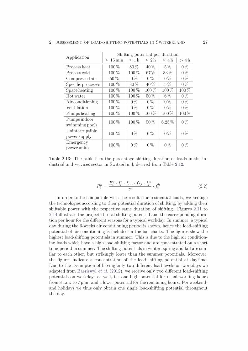
Table 2.13: The table lists the percentage shifting duration of loads in the in-dustrial and services sector in Switzerland, derived from Table 2.12.
P hi =
Eyi · fsi · fL,i · fI,i · fwi
ts· fhi (2.2)
In order to be compatible with the results for residential loads, we arrangethe technologies according to their potential duration of shifting, by adding theirshiftable power with the respective same duration of shifting. Figures 2.11 to2.14 illustrate the projected total shifting potential and the corresponding dura-tion per hour for the different seasons for a typical workday. In summer, a typicalday during the 6-weeks air conditioning period is shown, hence the load-shiftingpotential of air conditioning is included in the bar-charts. The figures show thehighest load-shifting potentials in summer. This is due to the high air condition-ing loads which have a high load-shifting factor and are concentrated on a shorttime-period in summer. The shifting-potentials in winter, spring and fall are sim-ilar to each other, but strikingly lower than the summer potentials. Moreover,the figures indicate a concentration of the load-shifting potential at daytime.Due to the assumption of having only two different load-levels on workdays weadapted from Baeriswyl et al. (2012), we receive only two different load-shiftingpotentials on workdays as well, i.e. one high potential for usual working hoursfrom 8 a.m. to 7 p.m. and a lower potential for the remaining hours. For weekend-and holidays we thus only obtain one single load-shifting potential throughoutthe day.

2. Assessment of load-shifting potentials in Switzerland 28
Hour [h]
Typical day in spring or fall, year 2020
Shiftable
pow
er[M
W]
Typical day in winter, year 2020
> 4 h≤ 4 h≤ 2 h1 h15 min
Typical day in summer, year 2020
1 2 3 4 5 6 7 8 9 10 11 12 13 14 15 16 17 18 19 20 21 22 23 24
1 2 3 4 5 6 7 8 9 10 11 12 13 14 15 16 17 18 19 20 21 22 23 24
1 2 3 4 5 6 7 8 9 10 11 12 13 14 15 16 17 18 19 20 21 22 23 24
0
500
1000
1500
0
500
1000
1500
0
1000
2000
3000
Figure 2.11: The figure shows the projected load-shifting potential of Swiss in-dustrial loads on a typical summer, winter, spring and fall workday in the year2020. Each hour, the left bar corresponds to the WWB scenario by Kirchneret al. (2012), the right bar to the NEP scenario. The exploitation via Smart-Meters in not yet considered.
We can therefore recognize a complementary occurrence of industrial andresidential load-shifting potential, both seasonally and hourly: Residential DSM-potentials are highest in winter and at night, whereas industrial DSM-potentialsare highest in summer and at daytime. Another opposing quality occurs, re-garding the shifting duration. The loads in the industrial and services sector canonly be shifted on shorter time-scales, while the residential sector offers longershifting durations.
Almost no change appears in industrial DSM-potential from 2020 until 2050in the WWB-scenario, as opposed to a decreasing trend in the NEP-scenario.Similarly to the residential case, in 2050 the NEP-scenario offers much less DSM-potential than the WWB-scenario. Both of these trends result from the projectedconsumption values (Kirchner et al., 2012), listed in Table 2.8.

2. Assessment of load-shifting potentials in Switzerland 29
Hour [h]
Typical day in spring or fall, year 2025
Shiftable
pow
er[M
W]
Typical day in winter, year 2025
> 4 h≤ 4 h≤ 2 h1 h15 min
Typical day in summer, year 2025
1 2 3 4 5 6 7 8 9 10 11 12 13 14 15 16 17 18 19 20 21 22 23 24
1 2 3 4 5 6 7 8 9 10 11 12 13 14 15 16 17 18 19 20 21 22 23 24
1 2 3 4 5 6 7 8 9 10 11 12 13 14 15 16 17 18 19 20 21 22 23 24
0
500
1000
1500
0
500
1000
1500
0
1000
2000
3000
Figure 2.12: The figure shows the projected load-shifting potential of Swiss in-dustrial loads on a typical summer, winter, spring and fall workday in the year2025. Each hour, the left bar corresponds to the WWB scenario by Kirchneret al. (2012), the right bar to the NEP scenario. The exploitation via Smart-Meters in not yet considered.
The here determined DSM-potentials in the industrial and services sectorare the part of the load, which could theoretically be shifted. In the followingmodel, the fraction that is actually exploited via AMM Smart-Meters is used.This fraction is based on the Smart-Meter rollout from Table 2.1.

2. Assessment of load-shifting potentials in Switzerland 30
Hour [h]
Typical day in spring or fall, year 2035
Shiftable
pow
er[M
W]
Typical day in winter, year 2035
> 4 h≤ 4 h≤ 2 h1 h15 min
Typical day in summer, year 2035
1 2 3 4 5 6 7 8 9 10 11 12 13 14 15 16 17 18 19 20 21 22 23 24
1 2 3 4 5 6 7 8 9 10 11 12 13 14 15 16 17 18 19 20 21 22 23 24
1 2 3 4 5 6 7 8 9 10 11 12 13 14 15 16 17 18 19 20 21 22 23 24
0
500
1000
1500
0
500
1000
1500
0
1000
2000
3000
Figure 2.13: The figure shows the projected load-shifting potential of Swiss in-dustrial loads on a typical summer, winter, spring and fall workday in the year2035. Each hour, the left bar corresponds to the WWB scenario by Kirchneret al. (2012), the right bar to the NEP scenario. The exploitation via Smart-Meters in not yet considered.

2. Assessment of load-shifting potentials in Switzerland 31
Hour [h]
Typical day in spring or fall, year 2050
Shiftable
pow
er[M
W]
Typical day in winter, year 2050
> 4 h≤ 4 h≤ 2 h1 h15 min
Typical day in summer, year 2050
1 2 3 4 5 6 7 8 9 10 11 12 13 14 15 16 17 18 19 20 21 22 23 24
1 2 3 4 5 6 7 8 9 10 11 12 13 14 15 16 17 18 19 20 21 22 23 24
1 2 3 4 5 6 7 8 9 10 11 12 13 14 15 16 17 18 19 20 21 22 23 24
0
500
1000
1500
0
500
1000
1500
0
1000
2000
3000
4000
Figure 2.14: The figure shows the projected load-shifting potential of Swiss in-dustrial loads on a typical summer, winter, spring and fall workday in the year2050. Each hour, the left bar corresponds to the WWB scenario by Kirchneret al. (2012), the right bar to the NEP scenario. The exploitation via Smart-Meters in not yet considered.

2. Assessment of load-shifting potentials in Switzerland 32
2.3 Transport sector
In 2010, around 95 % of the energy consumption in the transport sector wasmet by burning fossil fuels (Kirchner et al., 2012). The sector is therefore veryCO2 intense. According to Kemmler et al. (2014), the electricity consumptionin the transport sector in 2013 amounted to 11 PJ, of which less than 0.1 PJ wasconsumed by electric vehicles. However, electric vehicles are the only potentialload-shifting technology in this sector, as we consider electric loads of railways,trams and trolleys-buses to be inflexible, since they have to meet their schedules.
BFE differentiates between electric passenger cars (pure electric and hybrid),electric light (pure electric and hybrid) and heavy utility vehicles and electricmotorbikes. Table 2.14 lists the projected percentage of the total mileage for thedifferent vehicle categories for the years and scenarios relevant for this analysis.In Table 2.15, the total mileage per vehicle category is shown. The values areobtained from Kirchner et al. (2012).
Vehicle-type2020 2025 2035 2050
WWB NEP WWB NEP WWB NEP WWB NEP
Electric0.25 0.00 1.03 2.21 3.40 7.14 12.65 25.30
passenger cars
Plug-in hybrid0.25 0.50 1.03 2.21 3.40 7.14 13.80 27.60
passenger cars
Electric light0.00 0.75 0.71 2.82 1.98 7.26 3.15 9.90
utility vehicles
Plug-in hybrid0.00 0.75 0.71 2.82 1.98 7.26 2.80 8.80light utility
vehicles
Electric heavy0.00 4.00 0.50 8.00 2.00 16.0 5.00 28.00
utility vehicles
Electric7.00 10.00 10.00 19.00 15.00 37.00 20.00 70.00
motorbikes
Table 2.14: The table shows the projected percentage share of the total mileagefor the different vehicle categories from Kirchner et al. (2012).
Vehicle-type 2020 2025 2035 2050
Passenger cars 60.10 61.80 65.50 67.10
Light utility vehicles 3.90 4.10 4.40 4.50
Heavy utility vehicles 2.50 2.60 2.80 2.80
Motorbikes 2.70 2.85 3.20 3.30
Table 2.15: The table shows the projected yearly mileage for the different vehiclecategories in billion kilometers from Kirchner et al. (2012).

2. Assessment of load-shifting potentials in Switzerland 33
Season2020 2025 2035 2050
WWB NEP WWB NEP WWB NEP WWB NEP
Summer, spring or fall 0.07 0.36 0.29 1.02 0.95 2.81 3.18 7.66
Winter 0.07 0.37 0.34 1.15 1.19 3.31 4.26 9.71
Whole year 0.28 1.44 1.20 4.22 4.03 11.75 13.81 32.68
Table 2.16: The table shows the total electricity consumption of all electricvehicles in PJ for the different seasons and for the whole years.
750 electric passenger cars were registered in Switzerland in March 2012, withan average battery capacity of 24.5 kWh. Their average electricity consumptionwithout heating, amounted to 14.2 kWh/100km. Due to heating, the consump-tion in winter is around 50 % higher which leads to a winter-consumption of22.2 kWh/100km (Kirchner et al., 2012). According to Baeriswyl et al. (2012),plug-in hybrid electric passenger cars consume only 4 kWh of electricity per100km, as they use a combustion engine in parallel. Their battery capacitiesamount to around 5 kWh (Kirchner et al., 2012). For plug-in hybrid electricpassenger cars, we assume no change in electricity consumption in winter, as theheating is usually fed with waste heat from the combustion engine.
Figure 2.15: The figure shows the percentage parked passenger cars and therespective locations from Oldewurtel et al. (2013).
Kirchner et al. (2012) lists light pure electric utility vehicles with an averageconsumption of 25 kWh/100km. They suggest a consumption of 30 kWh/100kmfor plug-in hybrids if they run on battery. Since hybrids only use electricityfor 40 % of the distances covered, we get an average electricity consumption of12 kWh/100km. As reference values for heavy electric utility vehicles, we usethe Chinese electric buses with a consumption of 120 kWh/100 km and a batterycapacity of 300 kWh, described by Kirchner et al. (2012). Due to the high weightof utility vehicles, we suppose that most of the energy is used for moving thevehicle, hence no change between summer- and winter-consumption is assumed.

2. Assessment of load-shifting potentials in Switzerland 34
Comparing different electric motorbikes from Zero Motorcycles (2014), weobtain an average consumption of 6.74 kWh/100km. We further assume that themotorbike fleet consists of 50 % small electric scooters. Electric scooters consume3.68 kWh/100km on average (Erwin Muller GmbH, 2014). We therefore use acombined average consumption of electric motorbikes of 5.21 kWh/100km. Nousage of motorbikes and scooters in winter is assumed.
From the yearly mileage, the above introduced electricity consumption valuesper distance and the assumptions concerning seasonal changes and losses, weobtain the total seasonal and yearly consumption of electric vehicles listed inTable 2.16. The different winter consumption and driving patterns are appliedto the time, which usually is coldest in Switzerland, i. e. end of November untilend of February (MeteoSchweiz, 2015). In the NEP-scenario, a strong increase inthe electric vehicles’ total electricity consumption can be observed, which leadsto around half of today’s residential electricity consumption in 2050. For theWWB-scenario, smaller growth is expected.
Typical day in winter, year 2025
Hour [h]
Typical day in spring, summer and fall year 2025
Energy
consumption
in[%
]of
totaldaily
consumption
Typical day in winter, year 2020
Typical day in spring, summer and fall, year 2020
1 2 3 4 5 6 7 8 9 10 11 12 13 14 15 16 17 18 19 20 21 22 23 24
1 2 3 4 5 6 7 8 9 10 11 12 13 14 15 16 17 18 19 20 21 22 23 24
1 2 3 4 5 6 7 8 9 10 11 12 13 14 15 16 17 18 19 20 21 22 23 24
1 2 3 4 5 6 7 8 9 10 11 12 13 14 15 16 17 18 19 20 21 22 23 24
0
5
10
0
5
10
0
5
10
0
5
10
Figure 2.16: The figure shows the hourly load of the full electric vehicle fleet inpercent of the daily load for the WWB-scenario.
In order to estimate the DSM-potential, we need an idea on the parking situ-

2. Assessment of load-shifting potentials in Switzerland 35
Typical day in winter, year 2025
Hour [h]
Typical day in spring, summer and fall year 2025
Energy
consumption
in[%
]of
totaldaily
consumption
Typical day in winter, year 2020
Typical day in spring, summer and fall, year 2020
1 2 3 4 5 6 7 8 9 10 11 12 13 14 15 16 17 18 19 20 21 22 23 24
1 2 3 4 5 6 7 8 9 10 11 12 13 14 15 16 17 18 19 20 21 22 23 24
1 2 3 4 5 6 7 8 9 10 11 12 13 14 15 16 17 18 19 20 21 22 23 24
1 2 3 4 5 6 7 8 9 10 11 12 13 14 15 16 17 18 19 20 21 22 23 24
0
5
10
0
5
10
0
5
10
0
5
10
Figure 2.17: The figure shows the hourly load of the full electric vehicle fleet inpercent of the daily load for the NEP-scenario.
ation of the electric vehicles. It can be assumed that electric-vehicle owners havecharging opportunities at home, and electric utility vehicles also have chargingstations at their usual parking location. Baeriswyl et al. (2012) states that ”by2035, 75 % of the parkings will have a charging infrastructure”. Kirchner et al.(2012) give projections of the new built charging stations that peak at 2035. Weestimate the numbers of available charging stations at work, education and otherparkings to 10 % in 2020, 20 % in 2025 and 90 % in 2050.
Figure 2.15 shows the percentage of parked passenger cars and the respectivelocations on usual workdays; throughout the day, more than 80 % of the carsare parked. As stated previously, we assume charging opportunities of 10 % in2020, 20 % in 2025 and 90 % in 2050 at work, education and other parkings. Forhome parking, we assume an availability of 100 % of charging stations. Duringweekends and on holidays, we estimate that 90 % of the cars are parked at homethroughout the day. We further assume the same parking pattern for electricmotorbikes. For utility vehicles, we use a fraction of parked vehicles of 90 %between 7 p.m. and 7 a.m. , and 10 % between 7 a.m. and 7 p.m.. On weekend-

2. Assessment of load-shifting potentials in Switzerland 36
Typical day in winter, year 2050
Hour [h]
Typical day in spring, summer and fall year 2050
Energy
consumption
in[%
]of
totaldaily
consumption
Typical day in winter, year 2035
Typical day in spring, summer and fall, year 2035
1 2 3 4 5 6 7 8 9 10 11 12 13 14 15 16 17 18 19 20 21 22 23 24
1 2 3 4 5 6 7 8 9 10 11 12 13 14 15 16 17 18 19 20 21 22 23 24
1 2 3 4 5 6 7 8 9 10 11 12 13 14 15 16 17 18 19 20 21 22 23 24
1 2 3 4 5 6 7 8 9 10 11 12 13 14 15 16 17 18 19 20 21 22 23 24
0
5
0
5
0
5
10
0
5
10
Figure 2.18: The figure shows the hourly load of the full electric vehicle fleet inpercent of the daily load for the WWB-scenario.
and holidays, we assume that 90 % of utility vehicles are parked. From theseassumptions and Figure 2.15, we define daily profiles, which give the fraction ofparked vehicles for every hour during the day.
Kirchner et al. (2012) states that if ”400000 electric vehicles were charged inparallel with a charging power of 11 kW, this would lead to an additional loadof 4.4 GW, [...] which gives rise to a control-necessity of the charging behavior,depending on electricity supply”. It is therefore very likely that some kind ofSmart Charging applications will spread across the market in future, in order toprevent critical grid situations and expensive grid upgrades.
Daily shifting potential electric vehicles
According to Oldewurtel et al. (2013), the ”vehicle-to-grid (V2G)” approach,i.e. discharging the stored electricity in the batteries of electric vehicles backinto the grid, leads to fast battery degradation, hence reduced battery lifetime.We hence do not expect that this approach will establish. However, load-shifting

2. Assessment of load-shifting potentials in Switzerland 37
Typical day in winter, year 2050
Hour [h]
Typical day in spring, summer and fall year 2050
Energy
consumption
in[%
]of
totaldaily
consumption
Typical day in winter, year 2035
Typical day in spring, summer and fall, year 2035
1 2 3 4 5 6 7 8 9 10 11 12 13 14 15 16 17 18 19 20 21 22 23 24
1 2 3 4 5 6 7 8 9 10 11 12 13 14 15 16 17 18 19 20 21 22 23 24
1 2 3 4 5 6 7 8 9 10 11 12 13 14 15 16 17 18 19 20 21 22 23 24
1 2 3 4 5 6 7 8 9 10 11 12 13 14 15 16 17 18 19 20 21 22 23 24
0
5
10
0
5
10
0
5
10
0
5
10
Figure 2.19: The figure shows the hourly load of the full electric vehicle fleet inpercent of the daily load for the NEP-scenario.
with electric vehicles can still be achieved by shifting the charging hours. Trafficpatterns and user constraints allow for the use of 70 % of the connected vehicles’charging power for load shifting (Oldewurtel et al., 2013). This limitation isincorporated in the following calculation of DSM-potentials of electric vehicleswith the factor fC,i. We further assume that on weekdays, 3 times more kilome-ters are driven than on holidays and that 5 % losses occur during charging. Assuggested by Baeriswyl et al. (2012), we use a potential shifting duration of 4hours for all charging vehicles.
Using these assumptions, we can define relative daily power consumptionprofiles for the different types of electric vehicles. Representatively, Figures 2.16to 2.19 show the joined relative daily profiles of all electric vehicles on workdaysfor the different years and scenarios. On weekends and holidays, our assumptionsyield constant profiles. Comparing the figures, the profiles in the WWB-scenariosshow less variation than the profiles in the NEP-scenarios. This is due to thelower fraction of electric utility vehicles in the WWB-scenario, which are as-sumed to be on duty from 7 a.m. until 7 p.m.. Moreover, the profiles do not

2. Assessment of load-shifting potentials in Switzerland 38
Vehicle-typeSpring, summer
Winterand fall
electric passenger cars 66.6 33.3
plug-in hybrid passenger cars 75.0 25.0
light utility vehicles 75.0 25.0
heavy utility vehicles 75.0 25.0
motorbikes 100.0 0
Table 2.17: The table shows the percentage seasonal electricity consumption ofthe different electric vehicle-types.
show peaks in the evening, when many cars return to their main charging loca-tions. Even though this outcome is a result of our assumptions, it can be justifieddue to several reasons: First, the majority of the electric vehicle fleet is parkedthroughout the day (see Figure 2.15). Second, ”many trips are short and there-fore do not utilize the full battery range” (Oldewurtel et al., 2013). Third, theneeded charging time of many electric vehicles, especially electric utility vehicles,is very predictable and can hence be distributed evenly over many hours.
P hi =
Eyi · fsi · fC,i · fwi · f li
ts· fhi (2.3)
Formula (2.3) is used to calculate the hourly shiftable power P hi of electric ve-
hicles for the different seasons. Our previous assumptions lead to similar parkingsituations, but different electricity consumption in winter, than in spring, sum-mer and fall. This is incorporated in the calculation by the seasonal factor fsi .The seasonal factors of the single technologies are listed in Table 2.17. For cal-culating the length of a season in days ts, again 65 workdays per season are used.The hourly fraction fhi is obtained from the daily profiles of charging vehicles.fwi denotes the consumption differences between a workday and a weekend- orholiday; f li denotes the losses.
We furthermore have to consider that the energy consumed during a tripcannot be shifted to the time before the trip. For instance, according to Figure2.15 most vehicles return to their parking locations between 6 and 8 p.m.. Ouroptimization algorithm later considers shifting of load to the preceding hours.As the load of these returning vehicles cannot be shifted to the hours before8 p.m., we have to adjust the allowed duration of shifting for the hours after7 p.m., i.e. just after the trip. Each time P h
i increases compared to the precedinghour, the number of vehicles returning to their parking locations exceeds thenumber of vehicles leaving their parking locations. For the following explanation,∆P h
i0is the amount by by which P h
i0increases compared to the preceding hour.
It therefore represents the electric vehicles that just arrived to their parkinglocations. ∆P h
i0cannot be shifted to the preceding hours, as the preceding hours

2. Assessment of load-shifting potentials in Switzerland 39
Hour [h]
Typical day in winter, year 2025
Shiftable
pow
er[M
W]
Typical day in summer, year 2025
Typical day in winter, year 2020
> 4 h≤ 4 h≤ 2 h1 h
Typical day in summer, year 2020
1 2 3 4 5 6 7 8 9 10 11 12 13 14 15 16 17 18 19 20 21 22 23 24
1 2 3 4 5 6 7 8 9 10 11 12 13 14 15 16 17 18 19 20 21 22 23 24
1 2 3 4 5 6 7 8 9 10 11 12 13 14 15 16 17 18 19 20 21 22 23 24
1 2 3 4 5 6 7 8 9 10 11 12 13 14 15 16 17 18 19 20 21 22 23 24
0
100
200
0
100
200
0
30
60
90
0
30
60
Figure 2.20: The figure shows the estimated shifting potential of electric vehi-cles for the years 2020 and 2025 in [MW]. The left bar represents the WWB-scenario, the right bar represents the NEP-scenario. The exploitation via Smart-Meters/Smart-Charging in not yet considered.
are before the trip. We therefore have to reduce the shifting potential in hour i0by ∆P h
i0. In hour i0 +1, this amount can then be shifted for one hour maximum.
In hour i0 +2 it can be only shifted for 2 hours and so on. Moreover, the numberof the vehicles returning to their charging stations is unknown. We thereforeassume that every hour, 10 % of the calculated total shifting potential P h
i canonly be shifted for one hour and 10 % can only be shifted for 2 hours, in orderto incorporate the continuous fluctuation of parked electric vehicles.
The resulting shifting potentials of electric vehicles are depicted in Figures2.20 and 2.21. The shifting potentials are generally higher at night, as most ofthe vehicles are parked at their charging stations, while at daytime, the vehiclesmight be parked at locations without charging facilities. A strongly increasing

2. Assessment of load-shifting potentials in Switzerland 40
Hour [h]
Typical day in winter, year 2050
Shiftable
pow
er[M
W]
Typical day in summer, year 2050
Typical day in winter, year 2035
> 4 h≤ 4 h≤ 2 h1 h
Typical day in summer, year 2035
1 2 3 4 5 6 7 8 9 10 11 12 13 14 15 16 17 18 19 20 21 22 23 24
1 2 3 4 5 6 7 8 9 10 11 12 13 14 15 16 17 18 19 20 21 22 23 24
1 2 3 4 5 6 7 8 9 10 11 12 13 14 15 16 17 18 19 20 21 22 23 24
1 2 3 4 5 6 7 8 9 10 11 12 13 14 15 16 17 18 19 20 21 22 23 24
0
500
1000
1500
0
500
1000
0
200
400
600
0
200
400
Figure 2.21: The figure shows the estimated shifting potential of electric vehi-cles for the years 2035 and 2050 in [MW]. The left bar represents the WWB-scenario, the right bar represents the NEP-scenario. The exploitation via Smart-Meters/Smart-Charging in not yet considered.
trend in the shifting potential can be recognized in both the WWB-scenarioand the NEP-scenario. However, the DSM-potentials in the latter scenario aregenerally by the factor 2 bigger, than in the WWB-scenario.
In the latter model, for the exploitation via Smart-Meters/Smart-Chargingthe values from Table 2.1 are used again.
2.4 Pure load-shifting technologies
In this section, we present different pure energy storage technologies that po-tentially qualify for load-shifting. The BFE has published an extensive study

2. Assessment of load-shifting potentials in Switzerland 41
on the development of energy storage technologies in Switzerland, conducted byHewicker et al. (2013). We summarize some of their findings, limiting ourselvesto time-scales starting at 15 minutes, which eliminates flywheels, super capaci-tors and inductors from this analysis. An extensive database of global energystorage projects can be found in Sandia Corp. (2012).
Power storage technologies generate profit out of temporal electricity price-spreads; their profitability depends on their fixed and operational costs. Thefixed costs are determined mainly by the initial investment costs, which includethe costs of the device and the grid connection. The operational costs dependon the device’s efficiency. The graph in Figure 2.22 shows the projected costdevelopment of different storage technologies. Except for pumped hydro storageand compressed air energy storage, a decreasing trend can be recognized for alltechnologies.
Figure 2.22: The figure shows the projected trends in the cost of storage devicesfrom Hewicker et al. (2013).
Hewicker et al. (2013) states that a ”large-scale deployment of new energystorage appliances in Switzerland will become [...] necessary and reasonable after2035”. Similarly, Andersson et al. (2011) expect batteries to become competitivefor short-term storage in 2030.
Pumped hydro storage
Today, 99 % of the worlds electricity storage is accomplished by pumped hydrostorage, with a global installed generation capacity of around 127 GW. Pumpedhydro storage is generally limited by geographical requirements, i.e. mountainousregions. The technology offers a high efficiency of 70-85%, flexible generation(100-4000 MW) and storage capacity (500-15000 MWh) and a short reaction time

2. Assessment of load-shifting potentials in Switzerland 42
of seconds to minutes. The high fixed costs of pumped hydro plants of 600-2700 CHF/kW and 150-670 CHF/kWh come with long lifetimes, usually over 30years. This results in current fixed costs of 0.11 CHF/kWh, assuming one fullcycle per day. Due to the high storage capacities, pumped hydro storage qualifiesfor electricity storage on many time-scales, i.e. from seconds to weeks. (Hewickeret al., 2013)
The current Swiss pumped hydro plants generate around 1.6 TWh per year(Thurler, 2014), with a total pumping capacity of around 1400 MW (SWV, 2012).Generally, pumped hydro storage units create profit out of temporal electric-ity price-spreads. However, ”the profitability of the classic business model oftransforming baseload-power into peakload-power over the course of the day hasdecreased due to the shrinking price-spreads” in Switzerland (Hewicker et al.,2013). Nevertheless, some existing hydro storage plants are currently enlargedand new plants are under construction, resulting in a total pumping capacity ofaround 3500 MW in Switzerland in 2017 (Thurler, 2014).
Compressed air energy storage
Compressed Air Energy Storage (CAES) stores electric energy by pumping highpressure air into hermetically sealed reservoirs, e.g. underground salt mines. Theenergy can be regained by discharging the air through a gas turbine. Two largescale commercial plants are currently in use. The first one has been put intooperation in Huntorf, Germany in 1978, the second one in McIntosh, USA in1991. (Sandia Corp., 2012)
Heat losses limit the efficiency of diabatic devices to 50 %, while adiabatic de-vices can reach up to 70 %. Power levels between up to 1000 MW can be achievedand the reservoir sizes are flexible, depending on available mines. The two ex-isting plants have 870 (Huntorf) and 2860 MWh storage capacity. The reactiontime ranges between 8 and 14 minutes and the lifetime is usually longer than30 years. The fixed costs of of 600-1200 CHF/kW and 150-300 CHF/kWh resultin costs per cycled kilowatt-hour of 0.11 CHF/kWh (assuming one full cycle perday). Hence, the fixed cost per cycled kWh is similar to pumped hydro storage.(Hewicker et al., 2013)
Batteries
Due to the different requirements of electronic devices, many different batterytechnologies exist today. The Tables 2.18, 2.19 and 2.20 list properties of thetechnologies that are, according to Hewicker et al. (2013), most interesting forDSM in Switzerland. Several of these technologies are already in use for load-shifting. For instance, two wind-projects in Hawaii, USA store energy in lead-acid batteries; a 15 MW and 3.75 MWh battery is used in the Kahuku windparkand a 1.5 MW and 375 kWh battery is operated within the Kaheawa windproject.

2. Assessment of load-shifting potentials in Switzerland 43
Likewise, redox-flow-batteries are currently used in other windparks. (Hewickeret al., 2013) As European example, in Braderup, Germany a 2 MW and 3 MWhhybrid lithium-ion- and redox-flow-battery system is integrated in a windpark(Sandia Corp., 2012). Since July 2014, the Swiss energy-provider EKZ has beencommercially operating a 1 MW and 500 kWh lithium-ion battery in Zurich,providing primary frequency control. (EKZ, 2014)
TechnologyOptimum Energy- Power-
Efficiency Maximumdischarge density density
[%] cyclesfraction [%] [kWh/t] [W/kg]
Lithium- 20-40100-150 700-1300 95
≤ 20000ion 80 4000-10000
Lead-acid 80 25-45 100-500 80-85 600-1200
Nickel-80 60-90 500-1000 85-90 600-1200
cadmium
Vanadium-80 16-33 20-28 70-80 10000
redox-flow
Sodium-sulfur 100 100-200 160-220 70-80 10000-15000
Sodium-80
90-120 150-170 90-95 ≥ 2000nickel chloride 25-45 100-500 80-85
Table 2.18: The table lists important battery properties from Hewicker et al.(2013).
As Tables 2.18 and 2.20 show, the battery technologies have high efficienciesand fast reaction times. Compared to pumped hydro or CAES, batteries onlyhave small power-ratings and storage capacities. They therefore rather qualify forstorage on short time-scales. A high range of power-densities exists, depending onthe technology. The limiting factor of batteries are the high costs (see Table 2.19),consisting of costs for the storage-medium, the periphery and the converter,combined with the cycle-bound lifetimes (see Table 2.18). For some technologies,the converter costs can be even higher than the costs for the storage medium.However, the costs for the storage medium are expected to decrease considerably,as depicted in Figure 2.22. According to Hewicker et al. (2013), the fixed costsof most battery technologies amount to 0.25 to 0.35 CHF/kWh; with around0.55 CHF/kWh, lithium-ion batteries have the highest fixed costs. Anderssonet al. (2011) project overall costs for battery storage of 0.16 to 0.28 CHF/kWhin 2020, 0.08 to 0.14 CHF/kWh in 2035 and 0.05 to 0.08 CHF/kWh in 2050.They project battery storage to become cheaper than pumped hydro storagebetween 2035 and 2050. Figure 2.22 shows a different projection, expectingbattery storage to be still more expensive than pumped hydro and CAES in 2050.The figure furthermore indicates a constant cost-development of pumped hydroand CAES. Both sources anticipate vast cost reductions for battery storage.

2. Assessment of load-shifting potentials in Switzerland 44
Sodium-sulfur and Sodium-nickel chloride batteries have to be operated athigh temperatures, which might disqualify them for some applications. (Hewickeret al., 2013)
TechnologyCost components
Storage-medium Periphery Converter[CHF/kWh] [CHF/kW] [CHF/kW]
Lithium-ion 360-1200 36-360 120-240
Lead-acid 96-240 24 120-240
Nickel-cadmium 480 24-42 120-240
Vanadium-180-480 60-120 720-1800
redox-flow
Sodium-sulfur 180-480 24-60 120-240
Sodium-180-480 24-60 120-240
nickel chloride
Table 2.19: The table lists the different cost components of batteries fromHewicker et al. (2013).
TechnologyPower- Storage- Reaction-
rating [MW] capacity [MWh] time [s]
Lithium-ion 0.01-2 0.01-0.5 ≤ 1
Lead-acid 0.1-50 0.5-200 ≤ 1
Nickel-cadmium 0.5-27 0.003-6.75 ≤ 1
Vanadium-0.25-50 0.5-250 ≤ 1
redox-flow
Sodium-sulfur 1-50 1-380 1-60
Sodium-2-50 0.5-250 1-60
nickel chloride
Table 2.20: The table contains the ranges for power-rating, storage-capacity andtypical reaction times for important battery technologies from Hewicker et al.(2013).
Power-to-gas
The Power-to-gas technology is still under development, generally based on theelectrolysis of hydrogen, optionally followed by a methanation, which combineshydrogen and carbon dioxide into methane. As a Swiss example, the Renerg2-project was launched by Cabalzar (2014), developing a combined methanationand mobility approach. According to Sandia Corp. (2012), five hydrogen storagesystems with power ratings between 0.15 and 1 MW are already operational inGermany and France.

2. Assessment of load-shifting potentials in Switzerland 45
The two main advantages of this technology are the possible usage of thelarge existing natural gas infrastructure for storage and the possible long-term(seasonal) storage of electricity. The natural gas supply networks can carry ahydrogen fraction of up to 10 % without taking damage; more hydrogen can cor-rupt the sealing of compressors. In contrast, the methane-feed-in is unlimited.Methane has the further advantages of a higher energy density and less poten-tial of the formation of explosive gas-air-mixtures. The main drawback of thistechnology is the poor round-trip efficiency of 36 to 45 % for Power-to-hydrogenand 27 to 36 % for Power-to-methane. (Hewicker et al., 2013)
Electrothermal storage
Technologies for electrothermal storage have not yet passed the early develop-ment stage. They are based on a back-and-forth conversion of electricity intoheat, generally using water or molten salt as storage medium. According toHewicker et al. (2013), electrothermal storage could qualify for load-shifting, at-taining an efficiency of 55 to 65 % if the storage duration does not exceed a fewdays. This statement, however, is highly hypothetical.
The large scale electrothermal storage with molten salt might be promis-ing for solar thermal power plants in warm regions. A pilot project in GilaBend, Arizona uses such an installation to buffer the generated electricity andgenerate electricity well into the evening. Several similar projects have beenlaunched in Spain. However, the Swiss climate is not suited for such installa-tions. (Sandia Corp., 2012)In the USA, numerous small scale ice thermal storage projects have been im-plemented in combination with air conditioning (Sandia Corp., 2012). Here, noback-conversion of the thermal energy into electricity is intended. With increas-ing air conditioning consumption, this approach might become interesting forSwitzerland.

Chapter 3
Optimization approaches
46

3. Optimization approaches 47
In this chapter, the DSM-potentials from Chapter 2 are applied to calculatethe effect of load-shifting on the total Swiss load-profile. Load-shifting is modeledusing an optimization for each hour of a representative year. The optimizationproblem is solved using the MATLAB optimization function linprog.
Different ways to include the shiftable loads into the market and their ef-fect on the Swiss load-profile are assessed, using five different optimization ap-proaches:
• The market cost minimization approach models generation and load-shifting in an overall market cost minimizing manner.
• The load-dependent tariffs approach simulates load-shifting triggeredby higher electricity-prices in times of higher total load.
• In the day- and night-tariffs approach, load-shifting in the currentTOU-pricing structure is modeled.
• The real-time pricing approach models load-shifting, if end-users getaccess to prices on the wholesale market.
• The real-time pricing combined with load-dependent tariffs ap-proach simulates load-shifting, if end-users get access to prices on thewholesale market, but the price is increased in times of higher total load.
Furthermore, the effect of the future distribution of new technologies and changesin consumption on the initial Swiss load-profile are assessed. Therefore, wedetermine new typical load-profiles for the years and scenarios considered. Inthis context, the previously mentioned tool for simulating the effect of DSM andnew technologies on existing yearly load-, generation and exchange profiles isdeveloped for Swissgrid AG. This tool is aimed to be used on future generationand load-profiles and market cost data, derived by Swissgrid AG within theirpower system planning process.
The different optimization approaches neglect shifting on a 15-minute-scale,since the goal of this thesis is to calculate the effect of load-shifting on the hourlySwiss load-profile. Furthermore, neither load nor generation data with 15-minutetime-steps is available to public. However, by changing the time-steps and time-horizon, the same approach could be used for modeling 15-minute load-profiles.
The load-shifting potentials are handed to the optimization as a part of theload, which could be shifted to the preceding hours. For instance, shifting theload from one hour n to hour n − 3, reduces the load in hour n and increasesthe load in hour n − 3 by the same amount. The load-shifting potentials fromChapter 2 are hence implemented as negative lower bounds for load-reductionin hour n. This way, load-shifting that does not impair the end-user function ismodeled.

3. Optimization approaches 48
3.1 Underlying data
For the different optimization-approaches, the installed generation capacitiesand costs per generation-type are needed. Furthermore, hourly profiles of theload, the load-shifting potential, power generation from renewables and inflexiblesources as well as hourly profiles of the flows across the Swiss borders have to bedefined.
Table 3.1 shows the installed generation capacity per technology for theWWB- and the NEP-scenario. The respective projected marginal costs for thedifferent years are listed in Table 3.2. The data come from Kirchner et al.(2012). In order to cover the most extreme scenarios, for WWB, variant C (gas-fired combined-cycle power plants), and for NEP, variant E (only renewables andimports) are used. Again, the values for 2025 are calculated as the arithmeticmean of the years 2020 and 2030. Waste incineration plants and renewablecombined-cycle plants are included in the category renewables, since their in-stalled capacity is included in renewables in the study of Kirchner et al. (2012).The installed hydro run of river generation capacity is obtained from Filippini &Geissmann (2014). No future changes in the installed hydro run of river capacityare assumed, as we consider the run of river capacity in Switzerland to be fullyexploited.
Generation-type2020 2025 2035 2050
WWB NEP WWB NEP WWB NEP WWB NEP
Hydro 17.49 17.49 17.49 17.51 17.50 17.75 17.55 18.50of which run of river 4.38* 4.38* 4.38* 4.38* 4.38* 4.38* 4.38* 4.38*
Nuclear 3.0 3.0 2.4 2.4 0.0 0.0 0.0 0.0
Fossil thermal 0.5 0.0 1.55 0.0 4.25 0.0 4.5 0.0
Fossil combined0.75 0.75 0.75 0.75 0.75 0.75 0.75 0.75
cycle
Renewable 0.65 1.25 1.0 2.4 3.0 6.0 6.0 12.75
Exchange 4.2** 6.2** 4.2** 7.6** 7.2** 7.6** 7.2** 7.6**
Table 3.1: The table shows the projected installed capacity in GW per generationtechnology for the different scenarios WWB, variant C and NEP variant E.The data are estimated from the respective graphs in Kirchner et al. (2012).The values marked with * are based on Filippini & Geissmann (2014), the onesmarked with ** are based on ENTSO-E (2014).
The hourly load-profiles are obtained from ENTSO-E (2015). As a repre-sentative base load-profile for Switzerland, we use their profile of the year 2014.This underlying profile is then scaled according to Kirchner et al. (2012); theysimply divided their base load-profile by the sum of the individual values andthen multiplied it with the consumption of the year considered. We thereforescale the underlying profile, using the consumption values from Kirchner et al.

3. Optimization approaches 49
Generation-type2020 2025 2035 2050
WWB NEP WWB NEP WWB NEP WWB NEP
Hydro 8.9 8.9 9.2 9.2 9.8 9.8 9.8 9.9
Nuclear 6.0 6.0 6.45 6.45 0.0 0.0 0.0 0.0
Fossil thermal 13.6 0.0 13.45 0.0 13.2 0.0 13.9 0.0
Fossil combined28.0 28.6 30.45 32.0 33.7 37.1 34.7 39.5
cycle
Renewable 23.8 20.6 19.2 17.55 11.3 11.7 9.3 9.6
Exchange 5.9 5.9 5.95 6.75 5.2 10.7 5.2 13.4
Table 3.2: The table shows the projected average generation costs in Rp/kWhper generation technology for the different scenarios WWB, variant C and NEPvariant E from Kirchner et al. (2012).
(2012), listed in Table 3.3. We furthermore modify the profile in a way that itstarts with a Monday, which simplifies our later calculations. As 2014 startedwith a Wednesday, we copy day 6 and 7 (the first Monday and Tuesday) of theprofile and insert them again as day 1 and 2, shifting the rest of the profile for2 days.
2020 2025 2035 2050WWB NEP WWB NEP WWB NEP WWB NEP
Load 10.63 10.14 10.78 9.87 11.15 9.55 11.94 9.20Consumption 221.30 210.40 224.25 205.50 232.00 198.20 248.50 190.90
Table 3.3: The table shows the projected peak-load in GW and the projectedtotal yearly consumption in PJ for the different scenarios WWB and NEP fromKirchner et al. (2012).
For nuclear, fossil thermal and fossil combined cycle power plants, constraintson the ramp-rates are needed. According to Deutch & Moniz (2011), ”relativelynew nuclear reactors ramp asymmetrically: The plants can down-ramp 20% oftheir total output within an hour, but they require six to eight hours to rampup to full load again”. Furthermore ”natural gas-fired power plants provide thegreatest generation flexibility to mitigate large-scale penetration of intermittentrenewables with ramp-rates of 8% per minute. New natural gas combined-cycle(NGCC) plants continue to improve their capabilities for responding to the inter-mittency of renewable generation.” In the Swiss energy outlook 2050, the possiblefossil generation will be covered by waste incineration plants and combined cy-cle plants. In variant C, which is relevant for this thesis, the fraction of wasteincineration plants is very small. We therefore use the above cited ramp-ratefor natural gas-fired power plants for the category fossil thermal. From theirnumbers, we hence deduce the hourly ramp-rates listed in Table 3.4.
The installed transmission capacity for cross-border exchanges for the years

3. Optimization approaches 50
Generation-category down-ramping up-ramping
Nuclear 20 % 3.33 %
Fossil thermal 100 % 100 %
Fossil combined cycle 100 % 100 %
Table 3.4: The table shows the hourly ramp-rates for the generation categoriesnuclear, fossil thermal and fossil combined cycle in percent of the installed ca-pacity.
2020, 2025 and 2030 is obtained from ENTSO-E (2014). We relate their conser-vative scenarios Scenario A (2020 and 2025) and Vision 1 (2030) to the BFE-scenario WWB. Likewise, their best estimate scenarios Scenario B (2020 and2025) and Vision 3 (2030) are related to BFE-scenario NEP. As no informationon changes on the cross-border transmission capacities after 2030 is available,we use their 2030 values for the years 2035 and 2050 as well. The respectivetransmission capacities are included in Table 3.1.
We further use data on the cross border electricity exchange, as well as theNet Transfer Capacity (NTC) from ENTSO-E (2015). Again, the representativeyear 2014 is used. In order to define normalized profiles of the exchanges acrossthe Swiss borders, we divide the exchange profile from 2014 by the maximumNTC of the year 2014. Multiplying these normalized profiles with the installedcross-border transmission capacity of the respective year then gives the desiredexchange profiles. Table 3.1 lists the installed cross-border transmission capacityof the relevant years from ENTSO-E (2014). The exchange profiles are modified,in order to start with a Monday as well.
The hourly profiles of the load-shifting potential for the different scenariosare calculated with the approach, introduced in Chapter 2 of this thesis. Thisway, profiles of representative weeks in the four seasons are found. Performing alinear regression between these weeks, yearly profiles of the total DSM-potentialsare defined.
For the normalized power generation profile from renewables, we use datafrom the Swissgrid AG. This data is confidential and we hence manipulatedthe data by adding random values. Multiplying the normalized profile with theinstalled renewable generation capacity of the respective year (Table 3.1), weobtain the absolute yearly generation profile.
One approach furthermore needs the hourly spot-market prices. Here, theday-ahead price data for the year 2014 from EPEX Spot (2015a) is used. Wetransform the prices from Euros per MWh to Swiss Rappen per kWh by mul-tiplication with a factor of 0.12. Again, the profile is modified in order to startwith a Monday.

3. Optimization approaches 51
3.2 Effect of new technologies and changes in con-sumption on initial Swiss load-profiles
3.2.1 Data
As new technologies spread across the market, they imply changes in the elec-tricity consumption throughout the day. In the following, the load-profile beforeload-shifting is referred to as the initial load-profile. According to Baeriswyl et al.(2012), the distribution of Smart-Meters and consumer education will lead to amore sensible electricity consumption behavior of residential end-users. Theystate that information on efficient energy use will lead to a reduction of electric-ity consumption of 1 % in the first 5 years and an additional 0.33 % from year 5on. They further estimate that the most sensible 25 % of the Smart-Meter userswill reduce their electricity consumption by 3.7 % in the first five years plus anadditional 1.23 % in the following years. The remaining 75 % of Smart-Meterusers will realize savings of 2 % in the first five years and an additional 0.67 %thereafter. Furthermore, they assume that at least 90 % of the population willeither be reached by consumer education or have Smart-Meters. Summing upall the savings and applying the Smart-Meter rollout factors from Table 2.1 andthe previously stated assumptions related to consumer education, we obtain thetotal reduction of residential electricity consumption listed in Table 3.5.
Reducing the residential fraction of every hourly value of the used load-profilefrom ENTSO-E (2015) by the factors listed in the Table 3.5, we incorporate theenergy savings through more sensible residential consumer behavior into theload-profile.
Scenario 2020 2025 2035 2050
Reduction of WWB 1.01 % 1.39 % 1.55 % 1.82 %electricity consumption NEP 1.47 % 2.40 % 2.87 % 3.06 %
Table 3.5: The table shows the percentage savings in residential electricity con-sumption resulting from more sensible energy-use due to consumer educationand Smart-Meters. The data are extrapolated from Baeriswyl et al. (2012).
At the same time, the yearly electricity consumption per technology pro-jected by Kirchner et al. (2012) gives rise to changes in the shape of the initialload profiles. These changes are assessed hereinafter.
Residential loads
According to Table 2.2, a strong decreasing tendency is expected in residentialhot water and space heating consumption. This decreasing trend goes alongwith a strong increase in the respective heat-pump fraction. Furthermore, strong

3. Optimization approaches 52
growth is projected for the consumption of residential heating, ventilation andair conditioning. Lighting consumption will decrease significantly, whereas theconsumption of other devices will increase. We cannot determine daily profilesof other devices, as the devices are not specified. However, we assume their effectto be already included in the load-profile by scaling it according to the projectedchange in yearly consumption. The projected peak-load and yearly consumptionvalues from Kirchner et al. (2012) are listed in Table 3.3.
Typical day in spring or fall
Hour [h]
Typical day in winter
Energy
consumption
in[%
]of
totaldaily
consumption
Typical day in summer
1 2 3 4 5 6 7 8 9 10 11 12 13 14 15 16 17 18 19 20 21 22 23 24
1 2 3 4 5 6 7 8 9 10 11 12 13 14 15 16 17 18 19 20 21 22 23 24
1 2 3 4 5 6 7 8 9 10 11 12 13 14 15 16 17 18 19 20 21 22 23 24
0
5
10
15
0
5
10
15
0
10
20
Figure 3.1: The figure shows the estimated hourly consumption of Swiss residen-tial lighting loads on a typical summer-, winter-, spring- and fall-day, in percentof the total daily consumption.
In order to estimate the effect of changes in hot water, space heating, ventila-tion and air conditioning and lighting consumption on the initial load profile, weneed normalized yearly load-profiles for each of the 4 categories. These profilesare obtained by creating a yearly linear regression curve between the daily profilesof the technologies in Figures 2.1 to 2.4 and 3.1. The latter profile represents theEnglish lighting consumption obtained from Zimmermann et al. (2012), which

3. Optimization approaches 53
we use as no data are available for Switzerland. According to de Haan et al.(2012), 60 % of the yearly electricity consumption of lighting appliances occur inthe winter half year. We therefore assume that 20 % of the yearly consumptionoccurs in summer, 50 % in spring and fall, and 30 % in winter. This assumptionyields the seasonal factors 0.2 for summer, 0.25 for spring and fall and 0.3 forwinter. For hot water, we need both, the controlled and the uncontrolled profilelater on.
Industrial and service loads
In Chapter 2, we approximated profiles of industrial loads with only two differentlevels, similar to the approach of Baeriswyl et al. (2012).
According to Table 2.11, most of these technologies either do not vary sea-sonally, or are not projected to change their consumption much in the future(see Table 2.9). Based on our simplified profiles, we assume that if a technologydoes not vary seasonally, the changes to the load-profile are already included byscaling the load-profile according to the change in total consumption (see Table3.3). Furthermore, we assume that the shape of the load-profile is not altered bytechnologies that only change their consumption insignificantly. Applying thesetwo criteria for exclusion, we solely assess the effect of changes in space heatingand air conditioning in the industrial and services sector.
For these categories, we again define normalized yearly load-profiles per tech-nology; from the weekend-factors in Table 2.10, we define weekly profiles, by firstsetting all weekend hours and the hours on workdays from 8 p.m. to 7 a.m. equalto the weekend-factor. The remaining hours, i.e. the working hours are then setto 100 %. These weekly profiles are then applied for the full year, in order to getyearly profiles. Dividing the yearly profiles by the sum of all their entries, weobtain a yearly profile, relative to the yearly consumption. We do not perform ayearly regression for industrial and service loads, as we assume their load to bemuch more steady and less vulnerable to climatic effects. According to Baeriswylet al. (2012), industrial air conditioning is only operated for 6 weeks every year.As the operating weeks are not further specified, we assume air conditioning inthe weeks that usually have the highest temperatures in Switzerland, i. e. theweeks 28 to 33 (MeteoSchweiz, 2015). We set the air conditioning profile for theremaining weeks to zero.
Transport loads
The assumptions made in Section 2.3 lead to the workday load-profiles of thewhole electric vehicle fleet shown in Figures 2.16 - 2.19. On weekends, the load ofelectric vehicles is assumed to be constant, with 90 % of electric vehicles parkedthroughout the day. We therefore obtain constant daily profiles with 4.17 %of the full daily load in every hour. As we want to obtain normalized yearly

3. Optimization approaches 54
profiles, we have to modify the 4.17 % in order to account for the previously madeassumption, that on weekdays, 3 times more kilometers are driven. This resultsin a 3 times higher load on weekdays. We therefore use a constant weekend profileof 1.39 % in every hour. Arranging 5 weekdays and 2 weekend-days in series, wethen define weekly profiles for each season. Performing a yearly linear regressionleads to a yearly load profile of transport loads Lt. Normalizing Lt accordingto Formula (3.1), we obtain a normalized yearly profile lt for electric vehicles.In order to obtain a curve relative to the seasonal electricity consumption, nhere ranges over all hours in each season. As the profiles in the Figures 2.16 -2.19 differ both between years and between scenarios, we have to perform thiscalculation for every year and scenario separately.
lt,n =Lt,n∑n Lt,n
(3.1)
3.2.2 Calculation of new load-profiles
Having calculated the yearly load-profiles for each of the relevant residentialand industrial and service loads, their seasonal variation is incorporated by mul-tiplying every hourly value Ln with the corresponding seasonal factor fsn (seeTables 2.4 and 2.11 for the seasonal factors). The corresponding normalizedload-profiles per technology are calculated by dividing every hourly value by thesum of all hourly values. Formula (3.2) displays this calculation. The resultingcurve l contains the hourly consumption per technology, relative to the respec-tive yearly consumption. In the following Formulas, index n denotes the hour ofthe year, i the relevant residential, industrial and service load and t the loads inthe transport-sector, i. e. the joined electric vehicles.
li,n =Li,n · fsi,n∑n Li,n · fsi,n
(3.2)
Multiplying the normalized load-profiles of the relevant technologies with theyearly consumption values E in 2013 (see Table 2.2) and subtracting the resultfrom the 2014 Swiss load-profile from ENTSO-E (2015), we obtain a reduced 2014load-profile Lr
2014. We use 2013 consumptions, as these are the most recent valuesavailable to public. Formula (3.3) represents this step. We neglect the presentload of electric vehicles, as there exist only very few in Switzerland. Therefore,this calculation is only carried out for the relevant residential, industrial andservice loads.
Lrn,2014 = Ln,2014 −
∑i
Ei,2013 · li,n (3.3)

3. Optimization approaches 55
The reduced load-profile is then scaled to the new year y using the peak-loadsLpeak listed in Table 3.3.
Lrn,y = Lr
n,2014 ·Lpeak,y
max(Lrn,2014)
(3.4)
Adding the product of the normalized load profiles li and the consumptionof the year y, Ei,y (see Table 2.2) to Lr
n,y, we include the effect of the changes inthe relevant load-categories. Furthermore, the load of electric vehicles is addedin every hour as the product of the normalized transport load-profile lt and thecorresponding seasonal electricity consumption Es
t from Table 2.16.
The resulting profile is then scaled again, according to Formula (3.6) in orderto match the new profile with the desired yearly consumption Ey from Table3.3. Furthermore, the profile is reduced by the residential savings So
y of thecorresponding year y and scenario o from Table 3.5. The here needed residentialproportion of the total consumption fresidential is calculated from the respectiveyearly consumption values in the Tables 2.8, 2.2 and 2.16.
Ln,y = Lrn,y +
∑i
Ei,y · li,n + lt,n · Est (3.5)
Lon,y =
(Ln,y ·
Ey∑n Ln,y
)·(
1−Soy · fresidential
100
)(3.6)
As a last step, we include the change in control of hot water loads, as a partof them will be connected to Smart-Meters. The Smart-Meter rollout factorsin Table 2.1 give the fraction of hot water loads, which will be connected toa Smart-Meter. We move the load of this fraction from the ripple-controlledprofile (see Figure 2.2) to the uncontrolled profile (see Figure 2.3), by carryingout the calculation in Formula (3.7). This way, the part of the hot water loads,which is connected to a Smart-Meter, is moved to the time the energy is actuallyconsumed. The shifting of this part of the hot water load is then subject to theoptimization in the subsequent sections. The hot water loads without Smart-Meter-connection remain controlled via ripple-control.
Lo,newn,y = Lo
n,y + Ehotwater,y · (lhotwater,uncontrolled,n − lhotwater,controlled,n) (3.7)
3.3 Optimization basis
The algorithm we implement is based on a cost-minimization. Therefore, an op-timization problem with the objective function in Formula (3.8) is implemented.

3. Optimization approaches 56
The function represents the MATLAB linear optimization algorithm linprog. Thedecision variables xi include all generators G, load-shifting ∆L, power consumedby each storage technology Ls, generation by each storage technology Gs andeach storage technology’s state of charge SOC. C represents the total costs thatare minimized by the optimization, c the cost for each of the decision variables.c is zero for Ls and SOC, since these variables do not affect the total costs.
Index i ranges over all decision variables from hour 1 to the last hour on thetime-horizon. The results in this report are all based on a 16-hour time-horizon.The program implemented for Swissgrid AG however allows for a free choice ofdifferent time-horizons ranging from 8 to 48 hours.
C =imax∑i=1
xi · ci (3.8)
For the load-shifting decision variables of ∆Lj,k, a small cost factor for c isintroduced, representing the customers’ motivation barrier. This factor preventsthe load-shifting in cases of very small cost savings. We set the c for load-shiftingequal to -0.01 Rp/kWh. The negative sign is necessary, as the load-shifting ismodeled as a reduction of load.
The objective function (Formula (3.8)) is subject to several constraints, listedin Formulae (3.9) to (3.15). n denotes the hour in consideration. The equalityconstraint in Formula (3.9) defines that during each hour, generation and loadmust balance each other.
∑Gn
Gn +∑Gs
n
Gsn = Linitial
n +∑Lsn
Lsn + ∆Ln (3.9)
With Formulas (3.10) and (3.11), the limited ramp-rates ru (up-ramping)and rd (down-ramping) of the relevant generators are incorporated in the opti-mization problem. In the first hour of the year, the ramp-rate is set to 100 % ofthe installed capacity for all generators.
Gin −Gi
n−1 ≤ ru (3.10)
Gin−1 −Gi
n ≤ rd (3.11)
Formula (3.12) defines the hourly storage balances. Formula (3.13) limitsthe maximum generation from storage, which is equal to the state of charge. ηs
represents the storage technology’s round trip efficiency.
SOCn = SOCn−1 −Gsn + Ls
n · ηs (3.12)

3. Optimization approaches 57
Gsn ≤ SOCn−1 (3.13)
The power-to-gas technology does not necessarily require a re-electrificationand feed-in back into the electricity grid and has a very poor round-trip efficiency.We therefore do not model it as one of the storage technologies. It is insteadconsidered a part of the load and hence added to the initial load-profile (seeSection 3.2).
Formula (3.14) defines the lower and upper bounds for each decision variable.
xmini ≤ xi ≤ xmax
i (3.14)
The hourly load shifting potentials differ in their possible duration of shifting.The algorithm should allow the load-shifting potentials to be shifted for anyduration less or equal their maximum duration. E.g. the 2-hour shifting potentialcan be shifted for 1 or 2 hours, or partly for 1 and partly for 2 hours. This way,their full cost-saving potential can be exploited.
Therefore, the respective load-shifting potentials are split into several decisionvariables. E.g. the 2-hour shifting potential is modeled by 2 decision variables,one representing the load that is shifted for 1 hour, the other one representingthe load that is shifted for 2 hours.
Formula (3.15) includes the respective bounds in the optimization problem.The previously determined profiles of the DSM-potentials limit the reduction ofthe load, i.e. the down-shifting in every hour n. ∆Lj
n is thus negative and the ≥operator has to be used.
j∑k=1
∆Lj,kn ≥ ∆Lj
n (3.15)
Index j represents the duration category and k denotes the duration the loadis actually shifted. For example, ∆L4,3
n is the part of the 4-hour load-shiftingpotential in hour n, which is shifted to hour n− 3. Formula (3.16) describes thetotal change of the load in hour n due to load-shifting; the first term includes allthe down-shifted load, i. e. the load shifted from hour n to the preceding hours;the second term includes all the up-shifted load, hence the load shifted from thesucceeding hours to hour n.
∆Ln =∑j∈J
j∑k=1
∆Lj,kn −
∑j∈J∧k∈K|k≤j
∆Lj,kn+k
J = {1, 2, 4, 8}K = {1, 2...8}
(3.16)

3. Optimization approaches 58
From the results of the optimization, the new hourly load-profile Lnewn can be
calculated. Formula (3.17) represents this calculation. The shifted load ∆Lj,kn
includes the down-shifted load to the preceding hours, as well as the up-shiftedload from the succeeding hours.
Lnewn = Linitial
n + ∆Ln −∑Gs
n
Gsn +
∑Lsn
Lsn (3.17)
This whole optimization is carried out consecutively for each hour of the yearin consideration, simultaneously for all hours on the time-horizon. After havingfinished the optimization in one hour, the optimization program updates theremaining shifting potentials, the initial load and the box-constraints of the suc-ceeding hours according to the optimization results. Therefore, the optimizationrepresents model-predictive control.
This load-shifting and storage optimization-model is the basis for the suc-ceeding approaches. The different ways of including the load-shifting into themarket are assessed by changing the implementation of the generators in themodel. The decision variables’ box-constraints are defined according to Table3.6.
Decision variable xmini xmax
i
G0 or predefined Installed generation capacity
generation profile or predefined profile
Gs 0 Power rating
Ls 0 Power rating
SOC 0 Storage capacity
∆Lj Shiftable power0
per duration (negative)
Table 3.6: The table lists the origins of the lower and upper bounds of thedifferent decision variables.
3.4 Market cost minimization approach
In this approach, DSM is used to minimize the total market cost. Technically,this could be achieved by a centralized control strategy or an aggregation modelthat includes DSM in the market clearing mechanism, e.g. as a VPP. We herebyassess the potential demand-side flexibility the system could gain through load-shifting.
Pumped hydro and hydro storage power plants in this case are not operatedin a profit-maximizing manner. Instead, they contribute to the overall market

3. Optimization approaches 59
cost minimization by the willingness to sell electricity at their average generationcosts. As pumped hydro and hydro storage power plants are highly flexible intheir choice when to generate electricity, they tend to generate during hours withhigh electricity tariffs in order to maximize their profit, i.e. minimize their op-portunity costs. Therefore, our here presented approach does not reflect today’spractices. The model could however be an answer to the increasing need forflexibility in the power system, due to the growth in intermittent and inflexibleelectricity sources. Especially after the shutdown of the last Swiss nuclear powerplant in 2034, new operation principles might be needed.
Figure 3.2: The figure shows the pseudo merit order curve for Swiss hydro powerplants in 2013 from Filippini & Geissmann (2014). The vertical green dashedlines mark 25, 50 and 75 % of the installed generation capacity, the horizontallines mark the respective intersections with the pseudo merit order -curve.
We model this approach, using the optimization problem described by Formu-lae (3.8) to (3.17). All generation categories listed in Table 3.1 are implementedas decision variables in the optimization. Table 3.2 assigns average generationcosts to each generation category. For nuclear, fossil thermal and fossil com-bined cycle generation, the respective cost listed in the table is used for c. Forthe categories hydro run of river, renewables and exchange, c is set to zero, sincein this approach, these generation categories follow the preset generation profilesdescribed in Section 3.1. Their generation is hence fixed and their costs do notaffect the result of the optimization. This implementation is chosen since hydrorun of river, renewables and power exchanges are subject to external effects thatare not included in our model. Table 3.6 lists the origins of the lower and upper

3. Optimization approaches 60
bounds of the different decision variables, used in this approach.
The constrained ramp-rates of generators are implemented using Formulae(3.10) and (3.11). This constraint applies for the generation categories nuclear,fossil thermal and fossil combined cycle. However, effectively only nuclear powerplants are limited (see Table 3.4). Of the other generation categories, hydrorun of river, renewable and exchange follow preset generation profiles in thisoptimization. The hydro generation from pumping and storage is considered tobe very flexible, i.e. not constrained by ramp-rates.
In Switzerland, the residual load is usually supplied by pumped hydro andhydro storage power plants. However, not all hydro plants have exactly thesame generation costs and in Switzerland, 60 different hydro power companiesexist (Filippini & Geissmann, 2014). We therefore use a more complex modelof the distribution of generation costs over the hydro power plants. We alignthis model with the pseudo merit order curve assessed by Filippini & Geissmann(2014), which is shown in Figure 3.2. The curve illustrates an approximatedgeneration cost distribution of all Swiss hydro power plants in 2013.
According to Filippini & Geissmann (2014), run of river power plants havethe lowest generation costs. Cropping the left side of the curve, we thereforefind the merit order curve of the remaining hydro plants, i. e. pumped hydro andhydro storage. We then divide the curve by the average hydro generation costs in2013, in order to get a merit order curve relative to the average cost. Therefore,removing the 4.38 GW of installed run of river generation capacity from the curveand dividing the curve by 5.8 Rp/kWh, results in the curve shown in Figure 3.3.
Percentof
averagecost
[%]
Percent of generation capacity (cumulated) [%]
0 20 40 60 80 10090
100
110
120
130
140
150
160
170
Figure 3.3: The figure shows the approximated normalized (percentage) meritorder curve for pumped hydro and hydro storage power generation in Switzer-land.

3. Optimization approaches 61
The curve in Figure 3.3 includes 15 different price levels. Splitting the in-stalled hydro generation capacity (less run of river) from Table 3.1 into the 15respective parts and multiplying the curve with the average hydro generationcost from Table 3.2, we calculate hydro merit order curves for each of the yearsand scenarios considered. This way, the generation category pumped hydro andhydro storage is divided into 15 subcategories, each represented by one decisionvariable in the optimization.
3.5 Load-dependent tariffs approach
Another option to include load-shifting in the market is the introduction of load-dependent tariffs, i. e. charging customers less in low-load times and chargingthem more at high-load. Therefore, the customers have the incentive to switchon their loads in low-load time-periods. This approach is similar to so the calledpeak-shaving and valley-filling method.
We use the same algorithm as in Section 3.4, but with some modifications.In this model, the generation costs have to be high at high loads and low at lowloads. We do not consider generation profiles for this approach, but we modelgenerators that generate and sell the electricity exactly at the cost, the loadspay.
Again, the objective function in Formula (3.8) and the equality constraintsrepresenting the hourly system balances in Formula (3.9) are used. Storage, box-constraints and load-shifting are again modeled with Formulae (3.12) to (3.17).Ramp-rate constraints are neglected.
2020 2025 2035 2050WWB NEP WWB NEP WWB NEP WWB NEP
Electricity-25.70 27.10 26.75 28.85 29.30 32.1 28.80 33.60
prices
Table 3.7: The table shows the projected end-user electricity prices in Rp/kWh(real 2010 prices) for the different scenarios WWB and NEP from Kirchner et al.(2012).
In this approach, we replace the generation model from Section 3.4 with ageneration model, representing the load-dependent tariffs. I.e. the generationcosts have to be high at high load and low at low load. Therefore, generation inthis approach consists of a fixed and a flexible part. The generation capacity ofthe fixed part is set equal to the yearly minimum load value and covered by onesingle generator throughout the year. As this part is fixed for the whole year,it is not affected by the optimization. The corresponding cost-factor c is set tothe respective consumer electricity price in Table 3.7. The flexible part of the

3. Optimization approaches 62
generation covers all the remaining load.
We model the higher costs in times of high load by incorporating an additionalcost-factor for the flexible generation part. For the base-cost, the values fromTable 3.7 are used, which lists the projected average end-user electricity pricesfor the different years and scenarios from Kirchner et al. (2012). The entriesfor the year 2025 are interpolated linearly between the respective years 2020 and2030. Moreover, we assume an extra payment of 0.5 Rp per 0.5 GW of additionalgeneration. This principle leads to the additional payment curve of the flexiblegeneration part illustrated in Figure 3.4. We introduce 15 virtual generationcategories with the cost from Table 3.7 plus the additional payments shown inthe figure. This way, the higher price in times of higher load is incorporated inthe optimization.
Additional
pay
ment[R
p/k
Wh]
Comulated flexible generation capacity [GW]
0 1 2 3 4 5 6 7
0
1
2
3
4
5
6
7
Figure 3.4: The figure shows the assumed additional load-dependent payments.
For load-shifting and storage, the same assumptions as in Section 3.4 areused.
Since the optimization minimizes the total cost, this approach triggers load-shifting and storage operation which targets a reduction of peaks.
3.6 Day- and night-tariffs approach
Currently, common tariff-models in Switzerland include two different end-userelectricity prices. The customers have to pay different prices at day and night. Atnighttime the load is usually lower than at daytime, which gave rise to this tariff-model. According to EKZ (2013), the day-tariff between 6 a.m. and 10 p.m. isusually 50 % to 100 % higher than the night-tariff between 10 p.m. and 6 a.m..

3. Optimization approaches 63
This pricing model is a simple version of the previously described TOU-pricingapproach.
For this calculation, we use the projected prices from Table 3.7. However,we increase the prices at daytime by 25 % and reduce the prices at nighttimeby 25 %. We therefore assume the same ratio between day- and night-tariff astoday. This leads to the prices listed in Table 3.8.
2020 2025 2035 2050WWB NEP WWB NEP WWB NEP WWB NEP
Day-32.13 33.88 33.44 36.06 36.63 40.13 36.00 42.00
price
Night-19.28 20.33 20.06 21.64 21.98 24.08 21.60 25.20
price
Table 3.8: The table shows the projected end-user electricity prices at daytimeand at nighttime in Rp/kWh (real 2010 prices) for the different scenarios WWBand NEP from Kirchner et al. (2012).
This approach implies a tariff distinction between daytime and nighttimeonly. We therefore do not have to consider generation profiles for this approacheither. Instead, we model the day- and night-tariffs by removing all generationdecision variables but one. This remaining generator has an unlimited genera-tion capacity and sells electricity exactly at the respective day- or night-tarifffrom Table 3.7. In order to model the effect of load-shifting in this pricingenvironment, we again use the algorithm introduced in Section 3.3.
The optimization is still based on the objective function in Formula (3.8)and the equality constraints representing the hourly system balances in Formula(3.9). Formulae (3.12) to (3.17) represent storage, box-constraints and load-shifting. Ramp-rate constraints are not included in this approach.
3.7 Real-time pricing approach
Nowadays, due to the increasing market penetration of electricity from renewablesources, high electricity tariffs do not necessarily coincide with high load. Ifinflexible generation meets a lower load, the prices drop due to an oversupply:Since inflexible generators cannot be turned down on short notice without highfinancial effort, they prefer to continue generating. In extreme cases, this caneven lead to negative prices (on intraday-markets). Renewable generation isreckoned among inflexible generators as well, as their generation depends onexternal factors (mainly wind-speed and solar irradiation). (EPEX Spot, 2015b)Therefore, low prices could occur at high loads as well, if the respective inflexiblegeneration exceeds the load. In this context, it would be most appealing from

3. Optimization approaches 64
both an end-user’s as well as from a generator’s perspective, to shift the loadaccording to real-time spot-market prices. This pricing approach is commonlyreferred to as RTP.
The implementation of this approach is again based on the optimizationproblem, described by Formulae (3.8) to (3.17). However, we assume that theloads always have to pay the spot-market price and there is always a generatorwilling to sell the electricity at this price.
However, an increase in load causes an increase in the spot-market priceas well. Likewise, a load-decrease results in a shrinking spot-market price. Inorder to implement the related market-clearing mechanism, we introduce thefollowing 15 generation categories: One generator always sells electricity at thespot-market price. 7 generators are willing to sell electricity cheaper than thespot market price. The cheapest of those 7 categories sells electricity at thelowest spot-market price over the time-horizon. The price increases linearly overthe other 6 categories towards the spot-market price. The remaining 7 generatorsare willing to sell electricity at prices linearly increasing towards the maximumspot-market price over the time-horizon. Each of the 15 respective generationcategories is assigned 1 GW of generation capacity and represents one of thedecision variables x in the optimization problem, with the cost c.
An example of the resulting hourly merit order curve is depicted in Figure3.5. During the optimization, this curve is calculated consecutively for everyhour, according to the respective marginal costs and time-horizon.
Price
Cumulated generation capacity [GW]
0 5 10 150.5
1
1.5
2
2.5
3
Figure 3.5: The figure shows an example for the assumed merit order curve,i e. the price the loads have to pay, relative to the spot-market price.
In this approach, load-shifting and storage are modeled the same way as inSection 3.4 and ramp-rate constraints are neglected.
3. Optimization approaches 65
3.8 Real-time pricing combined with load-dependenttariffs approach
This approach is a combination of RTP (Section 3.7) and load-dependent tariffs(Section 3.5). Technically this approach again implies a transfer of the spot-market price to end-users. In order to prevent too high load peaks, which mightbe an outcome of the respective load-shifting, the corresponding system operatorscould charge the customers higher grid payments in times of high load.
In order to model this relation, we use the same spot-market based generationcost c as in the real-time pricing approach (Section 3.7). However, we add aload-dependent term to the price-distribution. This second term is zero for thefirst 5 GW and increases by 1 Rp/kWh for every additional GW between 6 and15 GW. We therefore model the generation again by 15 generation-categorieswith 1 GW of generation capacity each.
The optimization problem and the corresponding load-shifting and storagemodels are again described by Formulae (3.8) to (3.17), whereat ramp-rate con-straints are neglected.

Chapter 4
Results and Discussion
66

4. Results and Discussion 67
In this chapter, example results of the different approaches described in Chap-ter 3 are presented. As we examined yearly profiles, we have to limit this chapterto excerpts, which indicate our key-findings.
In Section 4.1, the results of the assessment of load-shifting potentials aresummarized.
Section 4.2 describes our findings concerning the effect of consumption changeson the initial load-profiles. Weekly examples of the resulting load-profiles arepresented.
The results of the different optimization approaches are described in Sections4.3 to 4.7. Comprehensive diagrams and tables for each optimization approach,scenario and year can be found in the appendix. As the future market penetrationof storage technologies is arguable, storage technologies are omitted in Sections4.3 to 4.7. However, in order to assess possible effects of storage on the load-profile, Section 4.8 describes optimization results with batteries and CAES forthe year 2050.
Section 4.9 completes this chapter with an analysis of the possible yearlysavings through DSM for representative end-users.
4.1 Assessment of load-shifting potentials
In Chapter 2, we assessed the DSM-potential of relevant technologies in thesectors residential, industrial and services and transport. Figures 4.1 to 4.4illustrate the resulting combined hourly shiftable power for the years 2020, 2025,2035 and 2050 for representative days in summer and winter. In the figures,the Smart-Meter rollout factors (see Table 2.1) are considered. The left barcorresponds to the WWB-scenario, the right bar to the NEP-scenario. Shiftingon time-scales below one hour are not considered here.
The figures indicate generally higher DSM-potential in winter than in sum-mer due to the heating loads, which are most suitable for shifting. The fasterexploitation of the DSM-potentials in the NEP-scenario, based on the faster dis-tribution of Smart-Meters, leads to higher hourly shiftable power in this scenario.In winter, the shiftable loads with longer duration are predominant, whereas insummer, all the four duration categories are about equally distributed.
In 2020, the hourly shiftable power in the WWB-scenario ranges between 30and 200 MW. It grows until 2050, to reach values between 200 and 1000 MW.The shifting potentials in the NEP-scenario are much higher: Already in 2020,an hourly shiftable power between 200 and 1300 MW is attained. Due to thevery swift Smart-Meter rollout, most of the DSM-potential is already accessiblein 2025, where the shiftable power ranges between 450 and 2400 MW. Until 2050,the DSM-potential does not increase anymore, as the overall electricity saving

4. Results and Discussion 68
2020 2025 2035 2050WWB NEP WWB NEP WWB NEP WWB NEP
Total electricity consumption [TWh]Residential 17.94 17.75 17.86 17.03 17.72 15.53 17.81 13.56Industrial and services 40.36 36.78 40.83 34.56 41.92 31.47 45.00 28.50Transport 0.08 0.40 0.33 1.17 1.12 3.26 3.84 9.08
of which shiftable [TWh]Residential 0.67 3.32 0.97 6.15 1.50 5.71 2.33 3.77Industrial and services 0.31 1.52 0.46 2.85 0.74 2.90 1.28 2.76Transport 0.004 0.11 0.03 0.63 0.16 2.04 0.98 6.14
of which shiftable [%]Residential 3.73 18.72 5.43 36.11 8.48 36.82 13.06 27.79Industrial and services 0.77 4.13 1.13 8.26 1.77 9.22 2.84 9.67Transport 5.09 26.43 8.18 54.04 14.25 62.36 25.57 67.60
of which shiftable [%] in case of full Smart-Meter rolloutResidential 46.58 46.79 45.26 45.14 42.42 40.91 37.32 29.25Industrial and services 9.67 10.33 9.42 10.33 8.86 10.25 8.12 10.18Transport 63.68 66.07 68.15 67.56 71.25 69.29 73.05 71.16
Table 4.1: The table shows the total electricity consumption and the shiftableenergy per sector. The values for the shiftable energy result from the analysis inChapter 2. The total electricity consumption originates in Kirchner et al. (2012).
measures compensate the better access to the shiftable power due to more Smart-Meters.
Table 4.1 lists the yearly electricity consumption, as well as the yearly shiftableenergy for the sectors residential, industrial and services and transport (electricvehicles). The values result from the assessment of DSM-potentials in Chapter 2.As for the optimizations, shifting with a duration below 1 hour is not considered.Due to the increasing Smart-Meter rollout factors (see Table 2.1), the shiftableenergy increases significantly towards the year 2050 in the WWB-scenario. Inthe NEP-scenario, the projected shiftable energy increases heavily until 2025,but then decreases again in the residential and the industrial and services sector,due to the projected decreasing overall consumption in these sectors.
Table 4.1 indicates the highest yearly electricity consumption in the industrialand services sector. However, the fraction of the consumption in this sectorwhich can theoretically be shifted is rather low, ranging between 0.77 and 9.67 %.Of the residential consumption, a higher fraction can be shifted. Here, thepercentage shiftable energy ranges between 3.73 and 36.82 %. In the transportsector, the highest fraction of the total electricity consumption can be used forDSM, reaching values up to 67.60 %. Looking at the absolute numbers, it canbe observed that for most scenarios and years, the residential sector holds thehighest DSM-potential. However, in the NEP-scenario, the shiftable energy ofelectric vehicles overtakes the shiftable energy in the residential sector in theyear 2050.

4. Results and Discussion 69
Hour [h]
Shiftable
pow
er[M
W]
Typical day in winter, year 2020
> 4 h≤ 4 h≤ 2 h≤ 1 h
Shiftable
pow
er[M
W]
Typical day in summer, year 2020
1 2 3 4 5 6 7 8 9 10 11 12 13 14 15 16 17 18 19 20 21 22 23 24
1 2 3 4 5 6 7 8 9 10 11 12 13 14 15 16 17 18 19 20 21 22 23 24
0
500
1000
1500
0
200
400
600
Figure 4.1: The figure shows the projected combined load-shifting potential ofSwiss loads on a typical summer- and winter-day in the year 2020. Each hour,the left bar corresponds to the WWB scenario by Kirchner et al. (2012), theright bar to the NEP scenario.
Later on, these values are also of interest in order to draw conclusions onthe economic attractiveness of DSM in the different approaches. The shiftablefraction of the total consumption in the case of a full Smart-Meter rollout inTable 4.1 is used for the succeeding evaluation of the possible yearly savings ofrepresentative end-users.

4. Results and Discussion 70
Hour [h]
Shiftable
pow
er[M
W]
Typical day in winter, year 2025
> 4 h≤ 4 h≤ 2 h≤ 1 h
Shiftable
pow
er[M
W]
Typical day in summer, year 2025
1 2 3 4 5 6 7 8 9 10 11 12 13 14 15 16 17 18 19 20 21 22 23 24
1 2 3 4 5 6 7 8 9 10 11 12 13 14 15 16 17 18 19 20 21 22 23 24
0
500
1000
1500
2000
2500
0
500
1000
1500
Figure 4.2: The figure shows the projected combined load-shifting potential ofSwiss loads on a typical summer- and winter-day in the year 2025. Each hour,the left bar corresponds to the WWB scenario by Kirchner et al. (2012), theright bar to the NEP scenario.

4. Results and Discussion 71
Hour [h]
Shiftable
pow
er[M
W]
Typical day in winter, year 2035
> 4 h≤ 4 h≤ 2 h≤ 1 h
Shiftable
pow
er[M
W]
Typical day in summer, year 2035
1 2 3 4 5 6 7 8 9 10 11 12 13 14 15 16 17 18 19 20 21 22 23 24
1 2 3 4 5 6 7 8 9 10 11 12 13 14 15 16 17 18 19 20 21 22 23 24
0
500
1000
1500
2000
2500
0
500
1000
1500
Figure 4.3: The figure shows the projected combined load-shifting potential ofSwiss loads on a typical summer- and winter-day in the year 2035. Each hour,the left bar corresponds to the WWB scenario by Kirchner et al. (2012), theright bar to the NEP scenario.

4. Results and Discussion 72
Hour [h]
Shiftable
pow
er[M
W]
Typical day in winter, year 2050
> 4 h≤ 4 h≤ 2 h≤ 1 h
Shiftable
pow
er[M
W]
Typical day in summer, year 2050
1 2 3 4 5 6 7 8 9 10 11 12 13 14 15 16 17 18 19 20 21 22 23 24
1 2 3 4 5 6 7 8 9 10 11 12 13 14 15 16 17 18 19 20 21 22 23 24
0
500
1000
1500
2000
2500
0
500
1000
1500
Figure 4.4: The figure shows the projected combined load-shifting potential ofSwiss loads on a typical summer- and winter-day in the year 2050. Each hour,the left bar corresponds to the WWB scenario by Kirchner et al. (2012), theright bar to the NEP scenario.

4. Results and Discussion 73
4.2 Effect of new technologies and changes in con-sumption on initial Swiss load-profiles
The projected reduction of residential energy consumption through Smart-Metersand consumer-education, listed in Table 3.5, leads to financial savings. Using theend-user electricity prices from Table 3.7 and the yearly residential consumptionfrom Table 2.2, we obtain the yearly savings listed in Table 4.2.
2020 2025 2035 2050WWB NEP WWB NEP WWB NEP WWB NEP
Cost-46.6 70.7 66.4 117.9 80.5 143.1 93.3 139.4
savings
Table 4.2: The table shows the projected combined yearly cost savings of allresidential end-users due to Smart-Meter- and consumer-education-triggeredchanges in consumption patterns. The values are in million Swiss Francs.
The Figures A.1 to A.8 in the appendix show the new load-profiles after ap-plying the calculation described in Section 3.2. The results are illustrated forone representative week for each season for both the scenarios WWB and NEPand the years 2020, 2025, 2035 and 2050. For winter, spring, summer and fall,the representative weeks 4, 17, 30 and 43 are chosen.Since all of the load-profiles were scaled in order to comply with the projectedyearly consumption values in Table 3.3, the initial and the processed profiles donot differ in their yearly consumption. However, the disproportional changesin the individual technologies imply changes on the shape of the load profiles.Nevertheless, according to Figures A.1 to A.8, the load-profiles keep their gen-eral shape with higher load at daytime on workdays and lower load at night andduring the weekend.
WWB-scenario
Figures A.1 to A.4 (appendix) indicate a decreasing trend of the consumed powerin the evening and night hours, especially for spring and fall, accompanied witha slightly increasing tendency at daytime. This effect can be explained withthe projected decrease in lighting and space heating energy consumption, whichpredominate in the evening and at night, and the increase in ventilation and airconditioning, which predominates at daytime. Additionally, a relative increase ofindustrial and service loads, compared to residential loads, supports this trend.Apparently, these effects outweigh the increase in evening- and night-load dueto electric vehicles.
Furthermore, a slight consumption-shift from spring and fall to summer andwinter can be observed. This shift might be due to the higher consumption of

4. Results and Discussion 74
ventilation and air conditioning in summer and electric vehicles in winter. Eachof these effects grows with time and is thus most distinct in the year 2050.
Today, the majority of hot water loads is shifted to night hours via ripplecontrol. Therefore, moving the part of the hot water loads that is now connectedto a Smart-Meter back to the time the energy is actually consumed by the end-user, reduces the load at night and increases it at daytime. This behavior isindicated by the red curves in Figures A.1 to A.4. Due to the hesitant rollout ofSmart-Meters in the WWB-scenario (see Table 2.1), this effect is less distinctivein the years 2020, 2025 and 2035.
NEP-scenario
According to Figures A.5 to A.8 (appendix), the decreasing trend of the con-sumed power in the evening and night hours and the increase at daytime can beobserved in the NEP-scenario as well. The consumption shift from spring andfall to summer and winter is also present. Since the changes in the respectiveconsumptions happen more quickly in this scenario, the two effects are morepronounced. Especially in the years 2035 and 2050, the deviation of the newcalculated (processed) profile from the base (unprocessed) profile become verydistinct. This implies a higher variation of the new load-profiles, with highermaximum and lower minimum values than the base profiles.
The lower total yearly consumption (see Table 3.3) leads to considerablylower hourly load values in the NEP-scenario than in the WWB-scenario.
Due to the very fast projected rollout of Smart-Meters (see Table 2.1), thedifferences between the load-profiles with and without controlled hot water aremuch larger in this scenario. However, the profile with uncontrolled boilers onlyrepresents an intermediate calculation step, as this profile is changed by thesubsequent optimization.
4.3 Market cost minimization approach
In this approach we analyze the effect of DSM on the load-profiles, if generationand load-shifting were operated in an overall market cost minimization manner.We now compare the optimization results for the different years and scenarios.
Changes to the load-profile
According to Figures A.9 to A.16 in the Appendix, the optimization in this ap-proach leads to shifting towards the hours with the highest electricity generationfrom renewables. Hence, load is shifted mainly to the hours around noon, wherethe renewable generation is highest. In the long run, this leads to load-peaksat noon. The operation of DSM for market cost minimization can lead to vast

4. Results and Discussion 75
improvements in the integration of renewables. Especially on longer time-scales,the DSM-potential is sufficient to greatly increase the utilization of the generatedrenewable electricity.
Yearly results
Table 4.3 lists main results of the optimization for the different years and scenar-ios. The table indicates an increase in the overall yearly peak-load due to shift-ing. This increase can be explained by the previously mentioned load-shiftingtowards the hours around noon, as this is already the usual peak-time withoutload-shifting. The maximum hourly shifted power ranges between 0.45 GW and2.74 GW and increases with growing total shiftable energy.
The table further shows that the total yearly savings and the savings pershifted unit are much higher in the NEP-scenario, than in the WWB-scenario.In the year 2050, the yearly savings due to load-shifting in the NEP-scenarioamount to around 140 million Swiss Francs. In this scenario, these savings are ashigh as the savings through residential efficiency improvements, listed in Table4.2. In the WWB-scenario, the resulting yearly savings through load-shiftingamount to less than 10 % of the possible efficiency-savings. This indicates thatthe possible savings through load-shifting depend on the amount of renewablesin the system: If there is a lot of electricity from renewables, the possible savingsthrough DSM are much higher, as DSM improves the utilization of renewablesand hence avoids generation from more expensive sources. Therefore, the use ofDSM for market cost minimization is more economically interesting in progressivescenarios towards renewables, such as the NEP-scenario.
According to Table 4.3, in the optimization only 26 to 48 % of the shiftableenergy is actually used for shifting. Comparing the different years and scenar-ios reveals that the more DSM-potential is available, the less energy is actuallyused for shifting, proportionally. The used fraction increases with the possibleduration of shifting, i.e. if a load can be shifted for longer time, it is more likelythat the shifting allows for an economical benefit.
Yearly results with restricted DSM-potentials
Table A.1 in the Appendix lists the yearly results of this optimization approach,if only the DSM-potentials of residential and industrial and service loads are usedand the DSM-potential of electric vehicles is omitted. Since, according to theprojections by Kirchner et al. (2012), the distribution of electric vehicles is stilllow in the years 2020, 2025 and 2035, the results for these years do not differ muchfrom the results in Table 4.3. However, in the year 2050, the possible savingsare much smaller, if electric vehicles are omitted. The total shiftable energy inthis year is much smaller, too, due to the high market impact of electric vehicles.Moreover, the fraction of the shifting potential that is actually used is slightly

4. Results and Discussion 76
2020 2025 2035 2050
WWB NEP WWB NEP WWB NEP WWB NEP
Total savings [million SFr.] 5.64 20.66 4.26 37.04 2.42 48.33 8.79 140.88
Average unit savings [Rp/kWh] 1.20 0.99 0.68 0.90 0.25 1.24 0.49 4.23
Total shiftable energy [GWh] 985 4948 1459 9638 2406 10656 4585 12660
Total shifted energy [GWh] 472 2084 629 4110 956 3908 1788 3333
Used shifting potential [%] 47.87 42.11 43.15 42.65 39.74 36.67 38.98 26.33
Peak-load without shifting [GW] 10.48 9.90 10.59 9.61 10.98 9.34 11.79 9.38
Peak-load with shifting [GW] 10.48 10.14 10.73 10.58 11.44 10.61 12.87 11.37
Maximum shifted power [GW] 0.45 1.13 0.55 1.76 1.08 1.99 1.63 2.74
1-h-shiftable energy [GWh] 95 465 145 937 255 1142 541 1609
Used 1-h-shifting [%] 42.57 27.92 34.95 26.51 29.22 20.70 25.32 15.86
2-h-shiftable energy [GWh] 306 1505 451 2843 725 2882 1259 2933
Used 2-h-shifting [%] 32.38 28.20 29.07 27.27 27.60 22.53 28.08 18.22
4-h-shiftable energy [GWh] 292 1496 439 3047 771 3867 1758 6135
Used 4-h-shifting [%] 46.70 41.67 42.43 42.70 38.74 37.47 39.20 26.58
8-h-shiftable energy [GWh] 292 1482 423 2811 655 2765 1028 1983
Used 8-h-shifting [%] 67.01 61.14 61.72 63.52 58.44 56.90 59.15 46.02
Table 4.3: The table shows the condensed yearly results of the market costminimization approach.
higher than if electric vehicles are included in the optimization. This supportsthe statement that an increase in DSM leads to a decreasing fraction of actuallyshifted load. The average savings per shifted kilowatt-hour are higher, than ifelectric vehicles are included. This leads to the insight that the savings pershifted unit are higher, if less DSM-potential is in the market.
In Table A.2 in the Appendix, the results of the optimization with onlythe DSM-potential of electric vehicles are shown. In the WWB-scenario, thetotal yearly shiftable energy of electric vehicles alone is comparably small inall years considered. This also implies low yearly savings through DSM. Inthe NEP-scenario, the shiftable energy grows more rapidly, due to the fasterdistribution of electric vehicles. Therefore, yearly savings due to shifting ofthe load of electric vehicles already become significant in this scenario in 2035.The table furthermore indicates that a very high fraction of up to 90 % of theshiftable energy is actually used for shifting, if the total shiftable energy is low.The savings per shifted kilowatt-hour are higher in the case with only electricvehicles, than in the case with residential and industrial and service loads only.As the case with only electric vehicles features the lowest yearly shiftable energy,this observation supports the theory that the savings per shifted unit are higher,if less overall DSM-potential is present in the system.

4. Results and Discussion 77
4.4 Load-dependent tariffs approach
The load-dependent tariffs approach models the effect of load-shifting triggeredby higher electricity-prices in times of higher total load in the power system. Theresults of the different scenarios and years considered are described hereinafter.
Changes to the load-profile
Figures A.17 to A.24 in the Appendix show the changes to the load-profile, re-sulting from the respective load-cost optimization for the scenarios WWB andNEP in the different years. According to the figures, this approach leads to thetypical peak-shaving and valley-filling behavior of such a peak-pricing mecha-nism. Therefore, load is generally shifted from daytime to nighttime and theload-profiles are generally flattened. This behavior is more distinctive in theNEP scenario, as here higher DSM-potentials are available sooner due to thefaster Smart-Meter rollout. Especially the results for the NEP-scenario in theyears 2035 and 2050, illustrated in Figures A.23 and A.24 (Appendix) show thatDSM in this scenario can flatten the profile significantly.
Yearly results
The load-profile flattening observation is reflected by the yearly peak-reductionshown in Table 4.4. Towards the year 2050, the reduction of the maximumyearly load value increases, especially in the NEP-scenario, as here more DSM-potential is available due to the higher Smart-Meter rollout. For the same reason,the yearly maximum hourly shifted power is higher in the NEP-scenario. Themaximum shifted power increases towards the year 2050, ranging between 0.39and 1.69 GW. The more DSM-potential is available, the higher the maximumhourly shifted power.
The yearly savings, as well as the average savings per shifted unit in thisapproach are a direct consequence of the assumptions concerning the additionalload-payment per additional total load-power. Therefore, these values are veryspeculative and hence not meaningful. As introduced in Section 3.5, our modelused an additional payment of 0.5 Rp/kWh per additional 0.5 GW. Using a higheradditional payment would result in higher savings. However, the results indicateaverage savings per shifted kilowatt-hour of 30 to 54 % of the additional paymentper additional 0.5 GW.
Table 4.4 further indicates that between 45 and 80 % of the total shiftableenergy are actually used in this approach. The used fraction decreases for bothscenarios with increasing DSM-potential. Moreover, the used fraction is highestfor the shifting potential with the longest possible duration of shifting. Hence,shifting potentials with a longer duration are more likely to allow for cost savings.

4. Results and Discussion 78
2020 2025 2035 2050
WWB NEP WWB NEP WWB NEP WWB NEP
Total savings [million SFr.] 1.76 4.78 2.39 6.54 3.75 8.14 7.47 16.16
Average unit savings [Rp/kWh] 0.23 0.17 0.22 0.13 0.22 0.15 0.26 0.28
Total shiftable energy [GWh] 985 4948 1459 9638 2406 10656 4585 12660
Total shifted energy [GWh] 780 2826 1109 4879 1706 5388 2829 5716
Used shifting potential [%] 79.16 57.12 76.00 50.62 70.89 50.56 61.71 45.15
Peak-load without shifting [GW] 10.48 9.90 10.59 9.61 10.98 9.34 11.79 9.38
Peak-load with shifting [GW] 10.40 9.47 10.46 9.30 10.65 8.90 11.40 8.88
Maximum shifted power [GW] 0.39 0.74 0.45 1.06 0.68 1.04 0.84 1.69
1-h-shiftable energy [GWh] 95 465 145 937 255 1142 541 1609
Used 1-h-shifting [%] 83.12 57.51 81.24 40.34 74.44 36.16 58.76 25.49
2-h-shiftable energy [GWh] 306 1505 451 2843 725 2882 1259 2933
Used 2-h-shifting [%] 71.06 40.01 66.21 32.78 59.29 33.76 50.67 32.12
4-h-shiftable energy [GWh] 292 1496 439 3047 771 3867 1758 6135
Used 4-h-shifting [%] 77.55 55.71 74.31 50.05 69.22 49.89 58.46 45.49
8-h-shiftable energy [GWh] 292 1482 423 2811 655 2765 1028 1983
Used 8-h-shifting [%] 87.98 75.78 86.41 72.70 84.31 74.95 82.31 79.32
Table 4.4: The table shows the condensed yearly results of the load-dependenttariffs approach.
Yearly results with restricted DSM-potentials
Table A.3 in the appendix shows the results of this approach with DSM of onlyresidential, industrial and service loads. The results for the years 2020, 2025and 2035 do not differ much from the results of the optimization with all DSM-potentials, due to the low distribution of electric vehicles in these years (seeKirchner et al. (2012)). In the year 2050, the omitted electric vehicles lead tolower available shifting potential, hence less shifting, less reductions of peaks andless savings. Furthermore, in the year 2050 the fraction of actually used shiftingpotential is higher, than if all DSM-potential was considered. This again impliesthat an increase in DSM leads to a decreasing fraction, which is actually shifted.
The results of an optimization with only the DSM-potential of electric ve-hicles are listed in Table A.4. Generally, the entries of the table support theprevious observations. Additionally, the savings per shifted kilowatt-hour in sce-nario WWB in 2020 are substantially higher, than in all other years in bothscenarios. For this specific case, we see very low total shiftable energy, of whichalmost 80 % are actually used for shifting. This indicates that the first shiftedunits lead to the highest savings and that DSM is the most attractive as longas only very little DSM-potential is actually in the market, i.e. early adopters ofDSM have an advantage.

4. Results and Discussion 79
4.5 Day- and night-tariffs approach
In the day- and night-tariffs approach, we analyze the effect of load-shifting onthe load-profiles, if the current day- and night-tariff model was kept. This impliesa higher price at daytime, i.e. between 6 a.m. and 10 p.m., than at nighttime. Inthe following, the optimization results for the different years and scenarios arecompared.
Changes to the load-profile
According to Figures A.25 to A.32 in the Appendix, the optimization in thisapproach generally leads to shifting towards early morning hours. In cases withonly low DSM-potential, this shifting pattern does not alter the load-profile toomuch. However, if high shiftable power is in the market, the load-shifting leadsto sharp peaks in the early morning hours. Especially in the NEP-scenario (seeFigures A.29 to A.32), these peaks are significant.
Yearly results
Table 4.5 lists the main results of this approach for the different years and scenar-ios. In the table, an increasing maximum yearly load value through load-shiftingcan be indicated, which grows with the total shifting potential. The maximumhourly shifted power ranges between 0.4 and 3.6 GW. The table indicates hightotal savings of up to 250 million Swiss Francs, if the DSM-potential is high.In the NEP-scenario in 2050, the total yearly savings are even higher than thesavings through residential efficiency improvements listed in Table 4.2. Savingsper kilowatt-hour of between 0.6 and 5.95 Rp/kWh can be observed, which alsoincrease with growing total shiftable energy. As the virtual generators in thisapproach represent the end-user tariffs, these savings refer to savings on the cus-tomers’ side only. This approach might not be realistic for scenarios with a lotof DSM-potential, as the associated high Smart-Meter rollout would allow formuch more advanced billing-models.
According to Table 4.5, in the WWB-scenario 73 to 94 % of the shiftable en-ergy are actually used. In the NEP-scenario, the used shifting potential amountsto only 33 to 60 %. A decreasing tendency from 2020 to 2050 can be recognized,which shows that the more DSM-potential is available, the less energy is actu-ally used for shifting, proportionally. The DSM-potential with a long duration ofshifting in preferred, as it is more likely that the shifting allows for an economicalbenefit.
Yearly results with restricted DSM-potentials
Table A.5 in the appendix lists the yearly results of the day- and night-tariffs ap-proach, if only the DSM-potential of residential and industrial and service loads

4. Results and Discussion 80
2020 2025 2035 2050
WWB NEP WWB NEP WWB NEP WWB NEP
Total savings [million SFr.] 5.61 28.49 9.12 63.57 17.73 99.73 43.58 249.35
Average unit savings [Rp/kWh] 0.60 0.96 0.67 1.66 0.83 2.34 1.30 5.95
Total shiftable energy [GWh] 985 4948 1459 9638 2406 10656 4585 12660
Total shifted energy [GWh] 933 2973 1365 3836 2124 4265 3349 4189
Used shifting potential [%] 94.73 60.10 93.55 39.80 88.29 40.02 73.03 33.09
Peak-load without shifting [GW] 10.48 9.90 10.59 9.61 10.98 9.34 11.79 9.38
Peak-load with shifting [GW] 10.50 10.06 10.60 11.96 11.00 11.86 11.88 11.94
Maximum shifted power [GW] 0.38 1.59 0.53 3.48 0.65 3.48 1.32 3.55
1-h-shiftable energy [GWh] 95 465 145 937 255 1142 541 1609
Used 1-h-shifting [%] 97.37 61.28 97.32 33.80 95.41 31.05 76.23 19.29
2-h-shiftable energy [GWh] 306 1505 451 2843 725 2882 1259 2933
Used 2-h-shifting [%] 93.75 32.04 90.96 18.92 80.35 21.45 66.09 23.87
4-h-shiftable energy [GWh] 292 1496 439 3047 771 3867 1758 6135
Used 4-h-shifting [%] 93.70 61.62 92.70 36.90 87.06 30.88 64.04 22.06
8-h-shiftable energy [GWh] 292 1482 423 2811 655 2765 1028 1983
Used 8-h-shifting [%] 95.92 86.68 95.89 66.04 95.73 75.87 95.21 92.05
Table 4.5: The table shows the condensed yearly results of the day- and night-tariffs approach.
are used and the DSM-potential of electric vehicles are omitted. Even thoughthis does not change the shiftable energy much, the yearly savings and the sav-ings per shifted unit in the years 2020, 2025 and 2035 are considerably reduced.This can be explained with the daily load-profile of electric vehicles, shown inFigures 2.16 and 2.17, which is favorable for shifting to the early morning hours.Moreover, the fraction of the shifting potential that is actually used is higher,than if electric vehicles are included in the optimization. This supports the state-ment that an increase in DSM leads to a decreasing fraction, which is actuallyshifted. The average savings per shifted kilowatt-hour are lower than if electricvehicles are included. This leads to the insight that in this particular approach,the shifting of the power of electric vehicles is more economically interesting,than shifting of residential, industrial and service loads.
This theory is supported by Table A.6, which shows the results of the opti-mization, if only the DSM-potential of electric vehicles is used. For this case, theactually used shifting potential increases over the years. The values are very high,ranging between 74 and 95 %. The savings per shifted kilowatt-hour increase aswell, if only electric vehicles are considered for DSM. Only in the NEP-scenarioin 2050 we see a comparably low fraction of used shiftable energy of 40 %, due tothe high overall DSM-potential in the market in this case. For this scenario andyear, the savings per shifted unit decrease as well, compared to the optimizationusing all DSM-potential. This can be explained by the use of one load-category

4. Results and Discussion 81
only: From a certain point, the uniform shape of the DSM-potential of electricvehicles, as well as the low values at daytime and in the evening, do not allowfor savings as high as the combined DSM-potential of various loads.
4.6 Real-time pricing approach
The real-time pricing approach models the effect of load-shifting triggered byRTP, i.e. end-user access to prices on the wholesale market. In the following,the results of the different scenarios and years are described.
Changes to the load-profile
Figures A.33 to A.40 in the appendix show the changes to the load-profile, im-plied by the respective end-user cost optimization. The figures indicate that thisapproach leads to sharp peaks in times of low spot-market prices. These peaksare already visible in cases with low DSM-potentials, such as the WWB-scenarioin 2020 or 2035. However, the peaks become more and more distinct, leadingto peaks drastically exceeding the initial load-profile in cases with high DSM-potential.
Yearly results
This observation of sharp load-peaks is reflected by the entries in Table 4.6, whichshows yearly results of the different scenarios and years analyzed. Especially inthe NEP-scenario, the table indicates high growth in the yearly maximum load-values. The growth ranges between 0.4 GW in cases with low DSM-potentialsand more than 2.3 GW in cases with high DSM-potential. Very high hourlymaximum shifted power of up to 4.4 GW can be observed.
Compared to the possible savings through residential efficiency improve-ments, the possible yearly savings in this approach are rather low in all casesconsidered. An increasing tendency with increasing DSM-potential is indicated.The average savings per shifted unit in this approach are rather low, rangingbetween 0.49 and 0.64 Rp/kWh.
Table 4.6 further shows almost no changes in the actually used shifting poten-tial. In all cases simulated, around 55 % of the total shiftable energy are actuallyused for shifting. This behavior can be explained by the fixed price curve, whichis used for all cases: This curve determines the hours with low electricity pricesand is equal in all cases. The table further indicates a preference of shiftingpotential with a longer duration, as shifting potentials with a longer possibleduration of shifting are more likely to allow for cost savings.

4. Results and Discussion 82
2020 2025 2035 2050
WWB NEP WWB NEP WWB NEP WWB NEP
Total savings [million SFr.] 3.64 16.15 5.26 27.54 8.32 29.80 14.98 39.62
Average unit savings [Rp/kWh] 0.64 0.57 0.63 0.50 0.61 0.49 0.59 0.58
Total shiftable energy [GWh] 985 4948 1459 9638 2406 10656 4585 12660
Total shifted energy [GWh] 572 2829 838 5478 1364 6026 2538 6867
Used shifting potential [%] 58.09 57.17 57.46 56.84 56.71 56.55 55.35 54.24
Peak-load without shifting [GW] 10.48 9.90 10.59 9.61 10.98 9.34 11.79 9.38
Peak-load with shifting [GW] 10.91 11.01 11.00 11.93 11.82 11.54 12.78 11.28
Maximum shifted power [GW] 0.82 2.93 1.05 3.78 1.54 3.98 2.48 4.40
1-h-shiftable energy [GWh] 95 465 145 937 255 1142 541 1609
Used 1-h-shifting [%] 49.89 47.94 48.67 47.70 47.60 46.71 45.62 45.54
2-h-shiftable energy [GWh] 306 1505 451 2843 725 2882 1259 2933
Used 2-h-shifting [%] 46.06 44.38 45.56 43.60 45.12 43.83 44.27 43.99
4-h-shiftable energy [GWh] 292 1496 439 3047 771 3867 1758 6135
Used 4-h-shifting [%] 55.70 54.41 55.16 54.12 54.75 54.36 54.56 54.37
8-h-shiftable energy [GWh] 292 1482 423 2811 655 2765 1028 1983
Used 8-h-shifting [%] 75.75 75.84 75.55 76.24 75.38 76.93 75.37 76.09
Table 4.6: The table shows the condensed yearly results of the real-time pricingapproach.
Yearly results with restricted DSM-potentials
Table A.7 in the appendix shows the results of this approach with the DSM-potential of only residential and industrial and service loads. The results for theyears 2020, 2025 and 2035 do not differ much from the results of the optimizationwith all DSM-potentials, due to the low distribution of electric vehicles in theseyears (see Kirchner et al. (2012)). In the year 2050, the omitted electric vehicleslead to lower available shifting potential, hence less shifting, slightly less increasein peaks and less savings.
The results of an optimization with only the DSM-potential of electric ve-hicles are listed in Table A.8. Increasing savings per shifted kilowatt-hour canbe observed, due to the lower total shiftable energy: The energy, that is actu-ally shifted can be shifted to the economically most attractive hours. Anotherinteresting finding is that in this case, the energy actually used for shifting islower in the NEP-scenario than in the WWB-scenario. This is due to the moreuniform profile of the DSM-potential of electric vehicles in the WWB-scenario,which offers higher shifting potentials at daytime. Due to the higher fraction ofelectric utility vehicles, which are not connected to charging stations during theday, DSM in the NEP-scenario can take less advantage of the low prices duringdaytime.

4. Results and Discussion 83
4.7 Real-time pricing combined with load-dependenttariffs approach
In this approach, we combined RTP with an additional payment in times of highload. We now compare the respective optimization results for the different yearsand scenarios.
Changes to the load-profile
According to Figures A.41 to A.48 in the appendix, the optimization leads inthis approach, similarly to the real-time pricing approach, to shifting towardsthe hours with the lowest electricity prices. However, the additional payment intimes of high load prevents the occurrence of sharp peaks and leads to a partialpeak-shaving and valley filling behavior. This heavily alters the shape of the re-sulting load-profiles in cases of high DSM-potential; in the NEP-scenario in 2050,the resulting load-profile almost does not show the typical day-and night-shapeanymore. It depends mostly on the spot-market price. This leads to the insight,that the DSM-potential in this case is high enough to achieve a very flexibleload-curve, which is highly volatile to price-signals.
Yearly results
Table 4.7 lists main results of the optimization for the different years and scenar-ios. The table indicates that the overall yearly peak-load only slightly increases inthis approach. In the NEP-scenario in 2050, the peak-load is even reduced. Themaximum hourly shifted power also decreases from 4.4 GW in the pure real-timepricing approach, to now 2 GW.
As in the load-dependent tariffs approach, the yearly savings, as well as thesavings per shifted unit are a consequence of the assumptions concerning theadditional payment in times of high loads. Therefore, these values are againspeculative. The results are based on the additional payment of 1 Rp/kWh peradditional gigawatt of load in the system, introduced in Section 3.8. However, itis not possible to identify, which part of the savings originates in an avoidanceof peak-load and which part in a shift towards low-price hours.
According to Table 4.7, in this optimization 51 to 59 % of the shiftable en-ergy is actually used for shifting. Comparing the different years and scenariosindicates that here, the actually shifted energy fraction only slightly decreaseswith growing DSM-potential. A preferential shifting over longer durations canagain be observed.
Yearly results with restricted DSM-potentials
Table A.9 in the appendix lists the yearly results of this optimization approach,

4. Results and Discussion 84
2020 2025 2035 2050
WWB NEP WWB NEP WWB NEP WWB NEP
Total savings [million SFr.] 4.67 16.16 6.54 24.06 9.99 27.07 17.91 41.62
Average unit savings [Rp/kWh] 0.80 0.58 0.76 0.46 0.72 0.47 0.70 0.64
Total shiftable energy [GWh] 985 4948 1459 9638 2406 10656 4585 12660
Total shifted energy [GWh] 585 2779 856 5213 1385 5739 2547 6517
Used shifting potential [%] 59.41 56.16 58.71 54.09 57.58 53.85 55.54 51.47
Peak-load without shifting [GW] 10.48 9.90 10.59 9.61 10.98 9.34 11.79 9.38
Peak-load with shifting [GW] 10.59 10.00 11.00 10.00 11.00 9.65 12.00 9.14
Maximum shifted power [GW] 0.78 1.49 0.96 1.83 1.10 1.74 1.25 2.00
1-h-shiftable energy [GWh] 95 465 145 937 255 1142 541 1609
Used 1-h-shifting [%] 51.16 46.18 50.10 41.78 48.92 39.56 45.48 36.42
2-h-shiftable energy [GWh] 306 1505 451 2843 725 2882 1259 2933
Used 2-h-shifting [%] 47.66 42.77 47.09 38.90 46.21 39.04 44.26 38.33
4-h-shiftable energy [GWh] 292 1496 439 3047 771 3867 1758 6135
Used 4-h-shifting [%] 57.65 54.42 56.94 53.13 56.19 53.79 55.60 53.83
8-h-shiftable energy [GWh] 292 1482 423 2811 655 2765 1028 1983
Used 8-h-shifting [%] 76.17 74.66 75.88 74.60 75.15 75.27 74.54 75.85
Table 4.7: The table shows the condensed yearly results of the real-time pricingwith load-dependent tariffs approach.
if only the DSM-potential of residential and industrial and service loads are used,and electric vehicles are omitted. In Table A.10, the results of the optimizationwith only the DSM of electric vehicles are shown. The tables indicate that inthis approach, electric vehicles alone allow for a good reduction of the overallyearly peaks. This peak-reduction is even higher than in the case with all DSM-potentials. The average savings per shifted unit are highest for the case with onlyelectric vehicles. This is due to the fact that, if only low DSM-potential is in themarket, it can take advantage of shifting in the hours that are economically mostattractive. I.e. higher competition reduces the possible savings through DSM.
4.8 Battery and CAES-storage
In Section 2.4, we assessed different storage technologies. We now analyze theeffect of high distributions of batteries and CAES, which are the two most promis-ing storage technologies apart from pumped hydro storage, on the Swiss load-profile. This thesis is generally based on the Swiss energy outlook 2050 byKirchner et al. (2012). However, the energy outlook does not include projectionsfor the development of storage technologies. We therefore use different hypo-thetical values for the installed generation and storage capacities, in order toanalyze possible effects of batteries and CAES on the load-profile. This analysis

4. Results and Discussion 85
is limited to the year 2050, as batteries and CAES are not expected to gain ahigh market penetration before 2035 (Andersson et al., 2011).
Assumptions
We use the previously introduced cost-projections of 0.05 CHF/kWh for batterystorage and 0.11 CHF/kWh for CAES in 2050 from Andersson et al. (2011) andHewicker et al. (2013). We here present the results of two different cases, onewith 4 GWh of installed battery storage capacity and 1 GW of battery powercapacity, and 2 GWh and 0.5 GW for CAES respectively. The other case is mod-eled with 1 GWh and 0.25 GW for batteries and 0.2 GWh and 0.05 GW for CAES.
Results
The results of the different optimization approaches of the two cases are illus-trated in Table 4.8 and 4.9; in order to assess the effect of storage, as well as re-ciprocal effects between storage and DSM, the tables list the optimization resultswith DSM and storage, with storage only and with DSM only. Again, the DSM-potentials are based on the results for the year 2050 in Chapter 2, i.e. 4585 GWhof total yearly shiftable energy in the WWB-scenario and 12660 GWh in theNEP-scenario.
The tables indicate that CAES is only used very sparsely in all cases, whereasbatteries are used heavily in the market cost minimization and in the day-and night tariffs approach. Therefore, the projected cost of CAES per cycledkilowatt-hour is still too high in 2050 to allow profitable operation, if the mar-ket develops as projected in the Swiss energy outlook 2050 by Kirchner et al.(2012). The tables further show that the price-spreads in the here modeled load-dependent tariffs and the two real-time pricing approaches are not high enoughto allow for profitable operation of batteries either.
The results for the market cost minimization approach indicate high uti-lization of batteries in the NEP-scenario, whereas the utilization in the WWB-scenario is significantly lower. Likewise, the possible yearly cost savings throughstorage are considerably higher in the NEP-scenario, than in the WWB-scenario.These two observations are again due to the higher amount of renewables in theNEP-scenario, which leads to higher price spreads; the batteries can be chargedin times renewables would otherwise be curtailed. The tables furthermore in-dicate a reduction of the savings through DSM per shifted unit, if storage isin the system. In turn, if both DSM and storage are in the system, the use ofbattery-storage is reduced by half, compared to the case with only storage. Stor-age therefore competes with load-shifting. Collating the two tables shows thatthe more storage in the system, the lower the savings per shifted unit becomefor DSM. Nevertheless, the total yearly market savings increase in both casesdue to battery storage. The amount of actually used shifting potential remains

4. Results and Discussion 86
Storage and DSM Storage only DSM only
WWB NEP WWB NEP WWB NEP
Market cost minimization approach
Total savings [million SFr.] 11.69 205.31 6.18 125.34 8.79 140.88
Total battery-generation [GWh] 26.55 652.18 57.99 1254.29 0.00 0.00
Total CAES-generation [GWh] 1.84 0.00 1.94 0.01 0.00 0.00
Average unit savings [Rp/kWh] 0.29 2.50 - - 0.49 4.23
Used shifting potential [%] 40.87 25.26 - - 38.98 26.33
Load-dependent tariffs approach
Total savings [million SFr.] 7.43 16.12 0.19 0.22 7.47 16.16
Total battery-generation [GWh] 0.13 0.10 0.16 0.08 0.00 0.00
Total CAES-generation [GWh] 0.04 0.04 0.04 0.03 0.00 0.00
Average unit savings [Rp/kWh] 0.26 0.27 - - 0.26 0.28
Used shifting potential [%] 61.83 45.80 - - 61.71 45.15
Day- and night-tariffs approach
Total savings [million SFr.] 236.23 474.13 192.67 224.92 43.58 249.35
Total battery-generation [GWh] 1456.00 1456.00 1456.07 1456.06 0.00 0.00
Total CAES-generation [GWh] 0.03 0.17 0.34 1.65 0.00 0.00
Average unit savings [Rp/kWh] 1.38 6.31 - - 1.30 5.95
Used shifting potential [%] 68.67 31.20 - - 73.03 33.09
Real-time pricing approach
Total savings [million SFr.] 15.65 40.27 1.13 1.68 14.98 39.62
Total battery-generation [GWh] 10.88 11.28 18.02 28.64 0.00 0.00
Total CAES-generation [GWh] 0.01 0.00 0.01 0.01 0.00 0.00
Average unit savings [Rp/kWh] 0.57 0.56 - - 0.59 0.58
Used shifting potential [%] 55.76 54.34 - - 55.35 54.24
Real-time pricing combined with load-dependent tariffs approach
Total savings [million SFr.] 19.92 41.99 6.49 3.82 17.91 41.62
Total battery-generation [GWh] 34.80 4.27 107.69 58.16 0.00 0.00
Total CAES-generation [GWh] 0.01 1.08 0.01 2.01 0.00 0.00
Average unit savings [Rp/kWh] 0.52 0.58 - - 0.70 0.64
Used shifting potential [%] 55.89 51.58 - - 55.54 51.47
Table 4.8: The table shows yearly results of the different optimization approachesin the year 2050 with DSM and storage, with storage only and with DSM only.The underlying storage- and power-capacities are 4 GWh and 1 GW for batteriesand 2 GWh and 0.5 GW for CAES.
almost unaffected by the storage in the system. Furthermore, the percentageactually used battery storage decreases with more storage in the system.

4. Results and Discussion 87
Storage and DSM Storage only DSM only
WWB NEP WWB NEP WWB NEP
Market cost minimization approach
Total savings [million SFr.] 9.84 162.56 2.87 46.21 8.79 140.88
Total battery-generation [GWh] 9.99 216.51 27.62 459.68 0.00 0.00
Total CAES-generation [GWh] 0.20 0.01 0.22 0.11 0.00 0.00
Average unit savings [Rp/kWh] 0.37 3.53 - - 0.49 4.23
Used shifting potential [%] 40.89 26.07 - - 38.98 26.33
Load-dependent tariffs approach
Total savings [million SFr.] 7.43 16.12 0.20 0.22 7.47 16.16
Total battery-generation [GWh] 0.12 0.09 0.15 0.08 0.00 0.00
Total CAES-generation [GWh] 0.03 0.02 0.03 0.02 0.00 0.00
Average unit savings [Rp/kWh] 0.25 0.27 - - 0.26 0.28
Used shifting potential [%] 62.94 46.11 - - 61.71 45.15
Day- and night-tariffs approach
Total savings [million SFr.] 91.73 305.63 48.17 56.40 43.58 249.35
Total battery-generation [GWh] 364.03 364.02 364.09 364.06 0.00 0.00
Total CAES-generation [GWh] 0.08 1.20 0.24 2.16 0.00 0.00
Average unit savings [Rp/kWh] 1.38 6.83 - - 1.30 5.95
Used shifting potential [%] 68.75 28.81 - - 73.03 33.09
Real-time pricing approach
Total savings [million SFr.] 15.22 39.80 0.49 0.74 14.98 39.62
Total battery-generation [GWh] 4.00 3.02 7.75 12.36 0.00 0.00
Total CAES-generation [GWh] 0.01 0.00 0.01 0.01 0.00 0.00
Average unit savings [Rp/kWh] 0.58 0.57 - - 0.59 0.58
Used shifting potential [%] 55.76 54.33 - - 55.35 54.24
Real-time pricing combined with load-dependent tariffs approach
Total savings [million SFr.] 19.27 41.74 3.90 2.46 17.91 41.62
Total battery-generation [GWh] 23.23 1.93 63.49 39.00 0.00 0.00
Total CAES-generation [GWh] 0.01 0.20 0.01 0.21 0.00 0.00
Average unit savings [Rp/kWh] 0.60 0.60 - - 0.70 0.64
Used shifting potential [%] 56.01 51.64 - - 55.54 51.47
Table 4.9: The table shows yearly results of the different optimization approachesin the year 2050 with DSM and storage, with storage only and with DSM only.The underlying storage- and power-capacities are 1 GWh and 0.25 GW for bat-teries and 0.2 GWh and 0.05 GW for CAES.
For the day- and night-tariffs approach, the table indicates major utilizationof batteries as well, and even higher savings than in the market cost minimization

4. Results and Discussion 88
approach. Here, the use of batteries does not differ between the two scenarios,as the savings are not influenced by the amount of renewables in the system,but only by the pricing structure. The savings through load-shifting in this ap-proach are not affected by the amount of storage in the system. Neither is thepercentage of actually used storage reduced due to more storage in the system.Generally, a TOU-pricing approach with such long low-price periods highly fa-vors the use of storage, as the devices can simply be charged during low-pricetimes and discharged during high-price times. As soon as the price-spread be-comes large enough, the storage can follow the pricing pattern. However, it hasto be borne in mind that the results here are a consequence of the previous pric-ing assumptions. A price-spread which is lower than the battery-costs per cycledkilowatt-hour would lead straight to needlessness of batteries in this approach.
Economical profitability of batteries
In the next step, we assess the possible economical profitability of a typicallithium-ion battery in the year 2050 in the two approaches discussed above. As-suming a battery storage capacity of 10 kWh and a power rating of 2.5 kW, thefindings in Section 2.4 lead to battery installation costs of around 3000 SwissFrancs. In the following, we further assume a lifetime of 10000 cycles. Our opti-mization results for 1 GWh of battery storage capacity and 0.25 GW of batterypower capacity in the system lead to around 210 battery-cycles per year in theNEP-scenario in the market cost minimization approach. In the case with stor-age and DSM in the system, this specific example battery could save around 215Swiss Francs per year and pay back the installation costs within 14 years, longbefore reaching the end of its lifetime. It would therefore be profitable. In theday- and night-tariffs approach with around 360 cycles per year and savings ofaround 560 Swiss Francs per year, the economic viability would be even better.However, as stated before, it is unlikely that this simple TOU-pricing structurewill still be present in 2050.
4.9 Possible savings for end-users
In this section we estimate the possible yearly financial savings through DSM andefficiency improvements of representative end-users in the different years, scenar-ios and approaches. We therefore assess the typical yearly electricity consump-tion of representative Swiss end-users and then apply the values from Table 4.1,in order to determine the shiftable fraction of their yearly consumption. Withthe percentage actually shifted energy and the calculated savings per shiftedkilowatt-hour, we estimate the possible yearly financial savings for the represen-tative end-users. For this estimation, we use the same representative end-usersfor all years and scenarios.

4. Results and Discussion 89
Representative end-users
According to Nipkow (2013), a typical household in an apartment block inSwitzerland consumes 2750 kWh of electricity per year and accommodates 2people. A typical single family house accommodates 4 people and consumes5200 kWh.
The electricity consumption of end-users in the industrial and services sectorin Switzerland varies heavily between different businesses, factory sizes etc. As anexample we use a commercial building from Aiulfi et al. (2010), which was builtin the 1990s and has a yearly electricity consumption of approximately 300 MWhwith an area of 27000 m2. As an industrial example, we use the factory of GnosisBioresearch SA in Locarno, listed in ProKilowatt (2014), with a yearly electricityconsumption of roughly 1350 MWh.
In order to estimate the yearly electricity consumption of a representativeelectric passenger car, we use values from Gindraux et al. (2013). For 2012,they specify a number of registered passenger cars of 4.3 million with a totalyearly mileage of roughly 90 billion kilometers. This leads to a yearly mileageper passenger car of around 21000 km. Using an average electricity consumptionof 16.2 kWh per 100 km (see Section 2.3), we obtain a yearly consumption ofaround 3400 kWh per electric passenger car.
Assumptions
From these yearly electricity consumptions, the respective shiftable fraction andthe average savings per shifted kilowatt-hour for the different approaches in Ta-bles 4.3 to 4.7, we can now estimate the possible yearly savings for each ofthe representative end-users. As an approximation for the fraction of the totalconsumption, each representative end-user can use for load-shifting, we use thevalues from Table 4.1. We assume that the shiftable fraction in case of a fullSmart-Meter rollout for each of the sectors reflects typical shiftable fractions ofindividual end-users in the corresponding sector as well.
Savings through DSM
Table 4.10 lists the resulting savings for the different approaches, scenarios andyears. However, as stated previously, the results for the load-dependent tariffsapproach and the real-time pricing and peak-shaving approach are a direct con-sequence of the assumptions concerning the additional payments in peak-times,taken in Chapter 3. Introducing higher additional payments can lead to muchgreater possible savings for the representative end-users in these approaches.
According to Baeriswyl et al. (2012), a Smart-Meter costs between 105 and145 Swiss Francs plus installation costs between 100 and 150 Francs. Theyfurthermore list a generic Smart-Meter lifetime of 18 years. In order to be eco-nomically attractive, the savings through Smart-Meters thus should be above 20
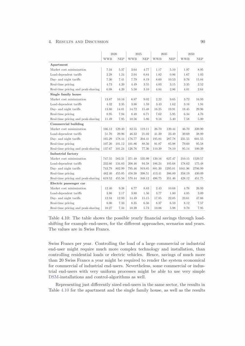
4. Results and Discussion 90
2020 2025 2035 2050
WWB NEP WWB NEP WWB NEP WWB NEP
Apartment
Market cost minimization 7.34 5.37 3.64 4.77 1.17 5.10 1.97 8.95
Load-dependent tariffs 2.28 1.24 2.04 0.84 1.82 0.86 1.67 1.03
Day- and night tariffs 7.30 7.41 7.79 8.19 8.60 10.53 9.76 15.84
Real-time pricing 4.73 4.20 4.49 3.55 4.03 3.15 3.35 2.52
Real-time pricing and peak-shaving 6.08 4.20 5.58 3.10 4.84 2.86 4.01 2.64
Single family house
Market cost minimization 13.87 10.16 6.87 9.02 2.22 9.65 3.72 16.93
Load-dependent tariffs 4.32 2.35 3.86 1.59 3.43 1.62 3.16 1.94
Day- and night tariffs 13.80 14.01 14.72 15.48 16.25 19.91 18.45 29.96
Real-time pricing 8.95 7.94 8.48 6.71 7.62 5.95 6.34 4.76
Real-time pricing and peak-shaving 11.49 7.95 10.56 5.86 9.16 5.40 7.58 5.00
Commercial building
Market cost minimization 166.12 129.40 82.55 119.11 26.70 139.44 46.70 339.90
Load-dependent tariffs 51.70 29.96 46.32 21.02 41.39 23.49 39.69 38.99
Day- and night tariffs 165.29 178.44 176.77 204.41 195.84 287.78 231.55 601.55
Real-time pricing 107.20 101.12 101.86 88.56 91.87 85.98 79.60 95.58
Real-time pricing and peak-shaving 137.67 101.24 126.76 77.36 110.39 78.10 95.14 100.39
Industrial factory
Market cost minimization 747.55 582.31 371.48 535.99 120.16 627.47 210.15 1529.57
Load-dependent tariffs 232.66 134.83 208.46 94.58 186.24 105.68 178.62 175.48
Day- and night tariffs 743.79 802.99 795.46 919.85 881.30 1295.01 1041.96 2706.99
Real-time pricing 482.40 455.05 458.38 398.51 413.41 386.89 358.19 430.09
Real-time pricing and peak-shaving 619.52 455.56 570.44 348.12 496.75 351.46 428.12 451.75
Electric passenger car
Market cost minimization 12.40 9.38 6.77 8.83 2.43 10.68 4.76 26.93
Load-dependent tariffs 3.86 2.17 3.80 1.56 3.77 1.80 4.05 3.09
Day- and night tariffs 12.34 12.93 14.49 15.15 17.85 22.05 23.61 47.66
Real-time pricing 8.00 7.33 8.35 6.56 8.37 6.59 8.12 7.57
Real-time pricing and peak-shaving 10.27 7.34 10.39 5.73 10.06 5.98 9.70 7.95
Table 4.10: The table shows the possible yearly financial savings through load-shifting for example end-users, for the different approaches, scenarios and years.The values are in Swiss Francs.
Swiss Francs per year. Controlling the load of a large commercial or industrialend-user might require much more complex technology and installation, thancontrolling residential loads or electric vehicles. Hence, savings of much morethan 20 Swiss Francs a year might be required to render the system economicalfor commercial of industrial end-users. Nevertheless, some commercial or indus-trial end-users with very uniform processes might be able to use very simpleDSM-installations and control-algorithms as well.
Representing just differently sized end-users in the same sector, the results inTable 4.10 for the apartment and the single family house, as well as the results

4. Results and Discussion 91
for the commercial building and the industrial factory are related. The resultsfor the electric passenger car show a similar progression as the results for therepresentative residential end-user, but are generally around 50 to 100 % higher.
A decreasing trend of the possible savings can be observed, due to the higherDSM-competition; if more DSM is in the market, a smaller fraction is actuallyshifted, which leads to lower savings. This yields an advantage for early DSM-adopters. In the market cost minimization approach, this trend is reversed inthe NEP-scenario, as here, the possible savings increase due to more renewablesin the system. Figure 4.5 illustrates these two opposed trends in the market costminimization approach, showing the possible yearly savings of the representativesingle family house, industrial factory and electric passenger car.
Year
Yearlysavings
inSFr.
Representative electric passenger car
Yearlysavings
inSFr. Representative industrial factory
NEP-scenarioWWB-scenario
Yearlysavings
inSFr.
Representative single family house
2020 2025 2035 2050
2020 2025 2035 2050
2020 2025 2035 2050
0
10
20
30
0
500
1000
1500
0
10
20
Figure 4.5: The figure shows the possible yearly savings through DSM of arepresentative single family house, industrial factory and electric passenger carin the market cost minimization approach.
The NEP-scenario offers higher savings for the end-users than the WWB-scenario in most cases in the market cost minimization and the day- and night-tariffs approach. In the load-dependent tariffs and the real-time pricing ap-proaches, higher savings can be achieved in the WWB-scenario. Overall, thehighest savings can be achieved within the day- and night-tariffs approach. How-ever, as stated previously, it is unlikely that the simple day- and night-tariff modelwill be kept, if a lot of DSM is in the system; this pricing model would not beprofitable for the respective utilities and could imply critical grid situations.

4. Results and Discussion 92
The results in Table 4.10 indicate that DSM can neither become economicallyviable for the representative residential end-users, nor for electric passenger carsalone, if the above introduced Smart-Meter and installation costs are considered;the possible yearly savings are in most cases well below 20 Swiss Francs. The onlyexception can be found for electric passenger cars in the market cost minimizationapproach in 2050, in the NEP-scenario1. However, adding an electric passengercar to a single family house can lead to savings above, or close to 20 Francsin many cases: This way, early adopters can achieve economically viable DSM-systems. Likewise, DSM can become profitable in the market cost minimizationapproach in 2035 in the NEP-scenario. If the example battery from Section 4.8was added to the end-user system in the year 2050 in the NEP-scenario, thiscould heavily enhance the economical attractiveness of the overall DSM, electricvehicle and battery system, if a market cost minimization approach was followed.
The possible yearly savings for the representative commercial and indus-trial end-users range between 21 and 1530 Swiss Francs per year2. Again, earlyadopters and users in the market cost minimization approach after 2035 canachieve the highest yearly savings through DSM. Regarding their high electric-ity consumption, the possible yearly savings are comparably low. However, DSMcan be economically attractive, if simple installation and operating principles areapplicable, i.e. the installation and equipment costs of DSM are low.
Efficiency-savings
As stated in Section 3.2, Smart-Meters enable residential customers to use theirelectricity more sensibly and therefore reduce their consumption. Accordingto Baeriswyl et al. (2012), the average end-user will reduce his consumptionby around 2.4 % in the first five years after acquiring a Smart-Meter. In thefollowing years, their projected reduction of consumption is even higher. For thetwo previously introduced representative residential customers, we can henceestimate the possible yearly savings due to a Smart-Meter-triggered reductionof consumption. The projected end-user electricity prices listed in Table 3.7,the estimated consumption reduction of 2.4 % and the yearly consumptions of atypical apartment and a typical single family house of 2750 kWh and 5200 kWh,yield the yearly financial savings listed in Table 4.11.
Table 4.11 indicates that the possible ”efficiency savings” of residential end-users due to Smart-Meters are much higher than the savings through DSM listedin Table 4.10. In the NEP-scenario, these savings alone could render Smart-Meters profitable already in 2020 for single family houses, and in 2035 for apart-ments, as savings of more than 20 Swiss Francs per year can be attained. In theWWB-scenario the savings are slightly lower due to the lower projected end-userelectricity prices. Here, efficiency savings of just below 20 Swiss Francs can be
1The day- and night-tariffs approach is assumed to vanish on the long run.2Neglecting the day-and night-tariffs approach after 2035

4. Results and Discussion 93
2020 2025 2035 2050
WWB NEP WWB NEP WWB NEP WWB NEP
Apartment 17.14 18.07 17.84 19.24 19.54 21.41 19.21 22.41
Single family house 32.41 34.17 33.73 36.38 36.95 40.48 36.32 42.37
Table 4.11: The table shows the projected yearly savings of representative res-idential Smart-Meter-users due to more sensible consumption behavior. Thevalues are in Swiss Francs.
gained. In single family houses, the Smart-Meters could become profitable in theWWB-scenario in 2020 as well.
However, these estimated yearly savings are a result of the projected devel-opment of the end-user prices from Kirchner et al. (2012). Depending on theDSM-implementation strategy and a more flexible demand side, these prices aresubject to change. Lower end-user prices would reduce these possible efficiencysavings. Furthermore, these savings do not come automatically but require someeffort on the customers’ side and a more sensible consumption of electricity doesnot necessarily need a Smart-Meter.

Chapter 5
Conclusion and Outlook
94

5. Conclusion and Outlook 95
In this thesis, we analyzed the possible impact of DSM on the hourly Swissload-profile in the years 2020, 2025, 2035 and 2050. The thesis is closely alignedwith the two different scenarios WWB and NEP by Kirchner et al. (2012) forthe development of the Swiss energy system. The WWB-scenario projects arestrained development, partially introducing fossil electricity sources, whereasthe NEP-scenario projects a very progressive development towards renewables.
This thesis considered DSM with timescales of one hour and above, since thegoal was to model the effect of DSM on the hourly load-profile for system plan-ning purposes. Therefore, load-shifting activity on ancillary-services markets wasomitted, as ancillary services are used to compensate for real-time imbalancesand do not affect the preceding generation and load scheduling.
DSM-potentials in Sitzerland
In order to simulate the effect of DSM on the Swiss load-profile, we definedhourly profiles of the shiftable power in Switzerland for all the years and scenariosconsidered. Comparing the resulting yearly shiftable energy of residential loads(see Table 4.1) with the results of the related analysis carried out by de Haanet al. (2012) (see Table 1.1), we found lower values. With a residential yearlyshiftable energy of 0.67 TWh in 2020, 1.5 TWh in 2035 and 2.33 TWh in 2050,our results are considerably below their estimation of around 9.5 TWh for 2020,2035 and 2050. In the progressive scenario we found 3.32 TWh in 2020, 5.71 TWhin 2035 and 3.77 TWh in 2050. Here our result for 2020 is also much lower thanthe 9 TWh by de Haan et al. (2012). For 2035 they projected a yearly residentialshiftable energy of 6.5 TWh; for 2050 they projected 4.3 TWh. These values aremuch closer to our results. The mismatches between our results and the reults ofde Haan et al. (2012) are mainly due to the different Smart-Meter rollout factorswe assumed. Especially in the restrained scenario, our lower rollout factors leadto lower shiftable energy. Their projection of a decreasing residential DSM-potential in the progressive scenario is supported by our results, which show adecreasing tendency after the year 2025 as well.The study of de Haan et al. (2012) is limited to the residential sector. Thisthesis expands their work, having assessed the DSM-potentials in the industrialand services and in the transport sector as well. We found the highest DSM-potentials in the residential sector until 2035. However, in the NEP-scenariothe DSM-potentials of electric vehicles can overtake the ones of the residentialsector. In the industrial and services sector, we determined high load-shiftingpotentials on short time-scales. Yet, the shiftable power with a possible durationof shifting of one hour or above is significantly smaller, than for residential loads.
Within their study on the impact of a distribution of Smart-Meters in Switzer-land, Baeriswyl et al. (2012) derived the hourly shiftable power of residential andindustrial loads and electric vehicles. In their conservative scenario, they pro-jected an hourly shiftable power of up to 300 MW in 2035, whereat they did not

5. Conclusion and Outlook 96
consider heating loads. Our results for the WWB-scenario yielded a shiftablepower in the range between 100 and 500 MW (see Figure 4.3), depending on thehour of the day and the season. Taking into account that we included heatingloads in the assessment, our results are comparable. In summer, when no heatingis present, we found a maximum value of 300 MW, too. The progressive scenarioby Baeriswyl et al. (2012) yielded an hourly shiftable power of up to 1382 MWin 2035. As Figure 4.3 shows, we found values between 500 and 2400 MW, againdepending on the hour of the day and the season. In summer we determineda maximum value of around 1300 MW. Our results are only higher due to theinclusion of heating loads, which increases the DSM-potential in winter. There-fore, our thesis generally supports their results.
Effects of DSM
Collectively, our assessment of the DSM-potential yielded similar values as thestudies by de Haan et al. (2012) and Baeriswyl et al. (2012). However, ouranalysis complements their work, not only providing general values of the yearlyshiftable energy and the hourly shiftable power, but assigning a DSM-potentialto every hour of the years we analyzed. Our results therefore show the seasonal,as well as the daily variation of the shiftable power. Our obtained profiles of thehourly shiftable power are well aligned with the Swiss energy outlook 2050 byKirchner et al. (2012). We provide a dataset for both their restrained scenario(WWB) and their progressive scenario (NEP). Altogether, we found that thetotal shiftable power in winter is around twice the shiftable power in summer.Furthermore, in winter the DSM-potential is highest at nighttime, whereas insummer, the DSM-potential at daytime is predominant.
Using the determined profiles of the hourly shiftable power, we modeled theeffect of DSM on the hourly load profile. Having assigned a possible durationof shifting to the hourly shiftable power, different cost-minimizing algorithmswere used to simulate the load-shifting. The considered duration of shifting wasthe time the load could be shifted, without affecting the end-user function. Thesimulation was therefore based on a previous filling of a reservoir, in order todeliver a service, i.e. an end-user function later on. Depending on the load-category, this reservoir could be any kind of storage, e.g. the temperature ofan air-conditioned room. The defined hourly load-shifting potentials for thedifferent years hence represent a condensed reservoir-model for the joined Swissload. The optimization was carried out consecutively for all hours of the yearin consideration, based on the condensed reservoir-model for the shifting of allloads. During each simulation step, the load-shifting of all hours on the time-horizon was optimized simultaneously.
As a main goal of this thesis, a tool was implemented for Swissgrid AG, al-lowing to apply the assessed hourly profiles of the DSM-potential within differentcontrol-strategies and incentives on various input data. The input data included

5. Conclusion and Outlook 97
power generation and exchange profiles as well as market data such as prices onthe wholesale-market. We therefore realized a tool which can quickly and easilymodel the effect of DSM on the Swissgrid data of future scenarios within theirtransmission system planning framework.
We implemented different optimization approaches in order to simulate theeffect of different strategies to control or incentivize DSM. We found that, ifDSM was used for market cost minimization, it can highly improve the integra-tion of renewables in the system. de Haan et al. (2012) got to the same result intheir study. The possible savings, both on a market-scale, as well as per shiftedunit in such an approach are highly dependent on the amount of renewables inthe system: With high generation from renewables in the system, vast savingscan be achieved through DSM. If the amount of renewables is small, DSM onlyenables low savings. This behavior is due to the low marginal costs of renew-ables. Improving their use allows for avoiding much more expensive generation.The analysis of possible cost savings for end-users revealed two opposing trends:Early adopters of DSM can gain higher savings, as they can actually use a higherfraction of their shiftable energy. With increasing DSM in the system, competi-tion leads to less use of the shiftable energy, which reduces the possible savings.Meanwhile, the previously explained relation with the amount of renewables inthe system leads to increasing possible savings over time. In the NEP-scenario,the increasing trend due to more renewables in the system predominates, which,in the long run, leads to economic viability of DSM. On the contrary, in theWWB-scenario the decreasing trend due to competition is dominant. Generalprofitability was also seen for industrial end-users, which yet depends on thecosts of the potentially more complex control installations.The analysis furthermore yielded the insight that in this approach, battery stor-age can become profitable in the year 2050 in the NEP-scenario. The possibleeconomic benefit here increases with the amount of renewables in the system aswell. We could therefore support the findings by Andersson et al. (2011), whoprojected battery storage to become economically viable after 2035. At large,such a DSM-approach could be implemented with centralized control strate-gies or hierarchical control via aggregators, which bid into wholesale-markets asVPPs.
Our analysis furthermore yields that the future DSM potential in Switzerlandis sufficient to lead to very flat load-profiles, if ”peak-shaving and valley filling”is incentivized. The prediction of load-behavior in such a DSM-implementationmight be simple and the expenses on the control infrastructure therefore couldbe small. However, with growing electricity-generation from photovoltaic cells indaytime, such an approach will probably be out-dated in future, as the reductionof day-load will no longer be an objective of DSM.Load-shifting triggered by the current Swiss TOU-pricing structure could allowfor high savings for end-users by shifting part of their daytime-consumption tothe night. Furthermore, battery storage could be highly profitable in such an

5. Conclusion and Outlook 98
approach. However, growing DSM-potentials can lead to sharp load-peaks in theearly morning hours if this pricing structure was kept. These peaks are caused bythe end-users’ tendency to shift their day-load to the early morning hours, whenthe electricity is still cheap. In Switzerland, the DSOs are responsible for end-user tariffs. Since they currently also take on the distribution of Smart-Meters,it is very unlikely that this simple and independent TOU-pricing will still bepresent if a high amount of DSM is in the system. The DSOs might rather in-troduce much more advanced pricing in order improve their system stability andavoid load-peaks. If a day- and night-tariff model is indeed maintained, the ratiobetween day- and night-tariffs might be reduced in order to prevent the unde-sirable occurrence of peaks due to load-shifting. A more elaborate TOU-pricingstructure might be implemented in future, in order to reflect the underlyingprices on the wholesale market.One problem of the current electricity billing-system is that the very steady end-user tariffs are almost fully independent from the fluctuating generation costs.An idea to improve this incoherent structure is to give end-users access to thewholesale market prices. Our results showed that such an approach can causehigh load-peaks in times of low prices as well, if it is not controlled appropriately.I.e. if all loads see the same price and optimize their demand accordingly with-out coordination, this can destabilize the system. The problem of an over- orunder-supply of the required response in the case of local decisions has alreadybeen described by Callaway & Hiskens (2011). In order to prevent this problem-atic, Borenstein et al. (2002) suggest a preceding anticipation of the customers’responses to price changes. This way, an end-user price that leads to a resultclose to the desired response could be achieved. Another possibility to avoid theoccurrence of sharp peaks is to introduce an additional payment in times of highload. Yet, our simulations imply that RTP does not render DSM profitable forend-users.
Summing up, our results showed a high impact of DSM on the Swiss load-profile. The way DSM is incentivized and controlled is crucial for the resultingeffect on the load-profile. Therefore, an appropriate strategy has to be found,in order to prevent negative effects of DSM on the power system, such as highload-peaks. In return, if DSM was introduced deliberately, it could be appliedto improve the utilization of renewables, provide system stability and enable fi-nancial savings.An economical advantage for early adopters of DSM could be observed. Withincreasing distribution of DSM, the fraction of shiftable energy that is actu-ally shifted, decreases due to competition. This results in a decreasing trend ofthe potential savings for end-users. However, if DSM was used to improve theutilization of renewables, an additional increasing trend of the possible savingsoccurs. In scenarios with a high amount of renewables, this increasing trend insavings outweighs the decrease due to competition. This leads to a good eco-nomical attractiveness of DSM for industrial and service end-users and those

5. Conclusion and Outlook 99
residential end-users who also possess an electric vehicle. In this case, batterystorage could as well become economically viable. Adding battery-storage to aDSM-installation could then lead to very profitable systems.Our analysis further showed that the yearly savings implied by Smart-Metersdue to more sensible consumption behavior of residential end-users can be muchhigher, than the savings through DSM. The same finding was already perceivedby de Haan et al. (2012). However, this outcome was based on the projecteddevelopment of end-user electricity prices from Kirchner et al. (2012). A moreflexible demand side might also lead to a reduction of end-user prices throughmarket forces, which would then reduce the possible residential savings throughconsumption-reduction. Moreover, our analysis showed that CAES will not be-come profitable in Switzerland until 2050.
5.1 Limits
Of the approaches we implemented, some are more realistic than others: it mightbe unlikely that an adequate control strategy will allow for using DSM for mar-ket cost minimization already in 2025, whereas it is promising in the long run.Analogically, it is not likely that the current TOU-model will be kept in timeswith high DSM in the market. However, this pricing-model might still be presentin 2025.
In the market cost minimization approach we simulated Switzerland alone, in-cluding the cross-border power exchanges as preset profiles. This approximationkeeps the optimization simple, but reduces the accuracy. A co-optimization ofSwitzerland an it’s neighbor countries would deliver more accurate results, butcomplicate the simulation. Such a co-optimization would also require a muchlarger dataset.
For the real-time pricing approaches, we used predefined profiles of the spot-market prices. The DSM-optimization was then carried out in order to mini-mize the end-user costs according to these predefined prices. The changes inspot-market price due to load-shifting were approximated during the simulation.However, in reality the spot-market clearing might already consider possible re-sponses of DSM. This would change the prices handed to the loads and possiblylead to more desirable load-shifting from a system operator’s perspective.
One issue we did not address in this thesis was data and infrastructure own-ership and the related data privacy protection. This issue might impede thedevelopment of DSM-potential.
Our analysis modeled the effect of load shifting on total Swiss load profile.Power system flows were not analyzed in this thesis. We optimized generationand load for the whole transmission system, assuming that all available load-shifting potential was utilized on a transmission system level. However, some
5. Conclusion and Outlook 100
of the load-shifting will presumably be used for optimizations on a distributionsystem level and hence be invisible to the TSO. Another part will very likely bebid into the ancillary services markets. Therefore, not all of the projected load-shifting potential will be available for an optimization on the transmission systemlevel. This thesis provides information on what could happen to the futuretransmission system. The effects in reality will probably be smaller. Therefore,an analysis of the distribution of DSM on different markets might be part of thefuture work. Nevertheless, the tool developed for Swissgrid AG allows for settingup simulations which only use the DSM-potential partially.
Generally, projections on very long time-scales, such as the scenarios for theyears 2035 and 2050 in the Swiss energy outlook 2050 by Kirchner et al. (2012),are subject to high uncertainties. This thesis is based on their projections. Forour estimation of available future load-shifting potentials as well as our differentoptimization approaches, we had to make several further assumptions. Therefore,this thesis modeled possible effects of load-shifting, rather than giving accuratepredictions for the future.
The real effect of load-shifting on the Swiss transmission system is highlydependent on the establishment of DSM regulations, markets and products. Itwill therefore be affected by decisions on a political level, as well as by influentialmarket players. As their behavior cannot be predicted impeccably, we modeleddifferent scenarios and concepts and based this thesis on data published by BFE.

Bibliography
Aiulfi, D., Maschio, I., Dellsperger, V., Brunet, L., Primas, A., Hagel, M., Benz-Karlstrom, P., Jakob, M., Honegger-Ott, A., & Grodofzig Furst, B. 2010. En-ergieverbrauch von Burogebauden und Grossverteilern. Bundesamt fur Energie(BFE), Bern, Switzerland.
Andersson, G., Boulouchos, K., & Bretschger, L. 2011. Energiezukunft Schweiz.Swiss Federal Institute of Technology (ETH), Zurich, Switzerland.
Baeriswyl, M., Muller, A., Rigassi, R., Rissi, C., Solenthaler, S., Staake, T., &Weisskopf, T. 2012. Folgeabschatzung einer Einfuhrung von Smart Meteringim Zusammenhang mit Smart Grids in der Schweiz. Bundesamt fur Energie(BFE), Bern, Switzerland.
Berner, D., Haller, M., Heimrich, S., Rumsch, W. C., & Rutishauser, D. 2014.FlexLast - Erzeugung von Sekundar-Regelenergie dirch ein dynamisches Last-management bei Grossverbrauchern. Bundesamt fur Energie (BFE), Bern,Switzerland.
BFE. 2011. Bundesrat beschliesst im Rahmen der neuen Energiestrategie schrit-tweisen Ausstieg aus der Kernenergie. Bundesamt fur Energie (BFE), Bern,Switzerland: Web. 22 Feb. 2015: https://www.news.admin.ch/message/
?lang=de&msg-id=39337.
BKW. 2015. Effiziente Energienutzung: Das ”Smart Metering”-Projekt in Ittigen(iSMART). BKW AG, Bern, Switzerland. Web. 2 Nov. 2014: http://www.
bkw.ch/ismart-ittigen.html.
Borenstein, S., Jaske, M., & Rosenfeld, A. 2002. Dynamic Pricing, AdvancedMetering, and Demand Response in Electricity Markets. eScholarship Repos-itory, University of California. Web. 15 Oct. 2014: http://escholarship.
org/uc/item/11w8d6m4.
Cabalzar, U. 2014. Projektvorstellung Renerg2. Swiss Federal Laboratories forMaterials Science and Technology (EMPA), Dubenborf, Switzerland. Web.15 Sept. 2014: http://www.iet.hsr.ch/fileadmin/user_upload/iet.hsr.ch/Bilder/Expertengespraeche_Cabalzar.pdf.
Callaway, D. S., & Hiskens, I. A. 2011. Achieving Controllability of ElectricLoads. Proceedings of the IEEE, Vol. 99, No. 1, pp. 184-199.
101

BIBLIOGRAPHY 102
CKW. 2011. Smart Metering Pilotprojekt: Positive Zwischenbilanz und neueAngebote. Centralschweizerische Kraftwerke AG, Luzern, Switzerland.Web. 12 Sept. 2014: http://www.axpo.com/axpo/hydrosurselva/de/
medien/medienmitteilungen/2011/juli/smart-metering-pilotprojekt-
positive-zwischenbilanz-und-neue-an.html.
de Haan, P., Bacher, R., Kissling, I., Fussen, D., Wolfensberger, M., Som-merhalder, M., & Zaugg, F. 2012. Flexibilisierung der Stromnachfrage inHaushalten. Verband Schweizerischer Elektrizitatsunternehmen (VSE), Aa-rau, Switzerland.
Deutch, J., & Moniz, E. 2011. Flexible operation of thermal power plants. TheMIT Energy Initiative’s Symposium on Managing Large-Scale Penetration ofIntermittent Renewables, pp. 23-29.
EKZ. 2013. EKZ fuhren flachendeckend Smart Metering ein. Elek-trizitatswerke des Kantons Zurich (EKZ), Zurich, Switzerland. Web.25 Sept. 2014: http://www.ekz.ch/content/ekz/de/ueberuns/medien/
medienmitteilungen/archiv2013/einfuehrung-smartmetering.html.
EKZ. 2014. EKZ Batteriespeicher ist offiziell am Markt fur Regelenergie.Elektrizitatswerke des Kantons Zurich (EKZ), Zurich, Switzerland. Web.01 Oct. 2014: http://www.ekz.ch/content/ekz/de/ueberuns/medien/
medienmitteilungen/archiv2014/batteriespeicher-am-markt/jcr:
content/rightPar/download/downloadList/132_1403020037623/file.
res/140701_MM_Batteriespeicher_Swissgrid.pdf.
Filippini, M., & Geissmann, T. 2014. Kostenstruktur und Kosteneffizienz derSchweizer Wasserkraft. Centre for Energy Policy and Economics (CEPE),Zurich, Switzerland.
Gindraux, M., Biedermann, F., Altwegg, D., Schnorr, K., Evequoz, R., Pittet,J., Marti, P., Bohnenblust, D., Gigon, C., Kesseli, G., Pool, M., Quandt, A.,Rebmann, K., Strahm, C., Beyeler, A., Bolliger, P., Fankhauser, A., Gonseth,C., Henriod, S., Muller, R., Rausa, F., Schurch, B., & Zecha, L. 2013. Mobilitatund Verkehr 2013. Bundesamt fur Statistik (BFS), Neuchatel, Switzerland.
Hewicker, C., Raadschelders, J., Werner, O., Ebert, M., Engelhardt, C., Men-nel, T., & Verhaegh, N. 2013. Energiespeicher in der Schweiz: Bedarf,Wirtschaftlichkeit und Rahmenbedingungen im Kontext der Energiestrategie2050. Bundesamt fur Energie (BFE), Bern, Switzerland.
Jordan, U., & Vajen, K. 2001. Realistic Domestic Hot-Water Profiles in DifferentTime Scales. Universitat Marburg, Marburg, Germany.
Kemmler, A., Piegsa, A., Ley, A., Keller, M., Jakob, M., & Catenazzi, G.2014. Analyse des schweizerischen Energieverbrauchs 2000 - 2013 nach Ver-wendungszwecken. Bundesamt fur Energie (BFE), Bern, Switzerland.

BIBLIOGRAPHY 103
Kirchner, A., Bredow, D., Ess, F., Grebel, T., Hofer, P., Kemmler, A., Ley, A.,Piegsa, A., Schutz, N., Strassburg, S., Struwe, J., & Keller, M. 2012. DieEnergieperspektiven fur die Schweiz bis 2050. Bundesamt fur Energie (BFE),Bern, Switzerland.
BKW AG. 2014. Innovative Losung zur Integration der ErneuerbarenEnergien. BKW AG, Bern, Switzerland. Web. 25 Sept. 2014:http://www.presseportal.ch/de/pm/100001009/100750601/bkw-
ag-netze-und-markt-innovative-loesung-zur-integration-der-
erneuerbaren-energien/rss.
ENTSO-E. 2014. ENTSO-E System Outlook and Adequacy forecast 2014-2030.European Network of Transmission System Operators of Electricity (ENTSO-E), Brussels, Belgium.
ENTSO-E. 2015. ENTSO-E Transparency platform. European Network of Trans-mission System Operators of Electricity (ENTSO-E), Brussels, Belgium. Web.2 Oct. 2014: https://transparency.entsoe.eu.
EPEX Spot. 2015a. European Power Exchange market data. European PowerExchange (EPEX) Spot, Paris, France. Web. 12 Jan. 2015: http://www.
epexspot.com/en/market-data.
EPEX Spot. 2015b. Negative Preise - Wie sie entstehen, was sie be-deuten. European Power Exchange (EPEX) Spot, Paris, France. Web. 28Jan. 2015: https://www.epexspot.com/de/Unternehmen/grundlagen_des_
stromhandels/negative_preise.
Erwin Muller GmbH. 2014. emco Elektroroller Kostenrechner.Erwin Muller GmbH, Lingen, Germany. Web. 7 Nov. 2014:http://www.emco-elektroroller.de/emco-elektroroller-modelle/
kostenrechner.html.
Sandia Corp. 2012. DOE Global Energy Storage Database. U.S. Depart-ment of Energy, Washington DC, USA. Web. 08 Apr. 2015: http://www.
energystorageexchange.org.
SWV. 2012. Pumpspeicherwerke sichern Netzstabilitat. SchweizerischerWasserwirtschaftsverbund (SWV), Baden, Switzerland. Web. 3 Nov.2014: http://www.swv.ch/Dokumente/Faktenblaetter-SWV-28Download-
Ordner29/Faktenblatt-Pumpspeicherung_SWV-2012.pdf.
Zero Motorcycles. 2014. zeroS-specs. Zero Motorcycles Inc., Scotts Valley, USA.Web. 7 Nov. 2014: http://www.zeromotorcycles.com/zero-s/specs.php.
MeteoSchweiz. 2015. Klimabulletin Jahr 2014. MeteoSchweiz, Zurich, Switzer-land.

BIBLIOGRAPHY 104
Morf, M. 2014. GridSense. Steuert Energie intelligent. Alpiq InTec Gruppe,Zurich, Switzerland. Web. 16 Sept. 2014: http://www.alpiq-intec.ch/
energie-effizienz/smarte-technologien/gridsense/gridsense.jsp.
Nipkow, J. 2013. Der typische Haushalt-Stromverbrauch. Schweizerische Agenturfur Energieffizienz (SAFE), Zurich, Switzerland.
Oldewurtel, F., Borsche, T., Bucher, M., Fortenbacher, P., Gonzalez Vaya, M.,Haring, T., Mathieu, J. L., Megel, O., Vrettos, E., & Andersson, G. 2013.A Framework for and Assessment of Demand Response and Energy Storagein Power Systems. IEEE, Bulk Power System Dynamics and Control - IXOptimization, Security and Control of the Emerging Power Grid (IREP), 2013IREP Symposium, pp. 1-24.
ProKilowatt. 2014. Funfte Wettbewerbliche Ausschreibungen fur Strom-effizienz 2014 - Kurzbeschreibungen bewilligte Projekte 2014. Bun-desamt fur Energie (BFE), Bern, Switzerland. Web. 28 Feb. 2015:http://www.bfe.admin.ch/php/modules/publikationen/stream.php?
extlang=de&name=de_238378629.pdf.
Swisscom. 2015. With over 4,500 people taking part, the tiko smart storage net-work is the first active smart grid in the Swiss market. Swisscom AG, Bern,Switzerland. Web. 3 Nov. 2014: https://www.swisscom.ch/en/about/
medien/press-releases/2015/02/20150210-MM-Speichernetzwerk-
tiko.html.
Thurler, G. 2014. Statistik der Wasserkraftanlagen in der Schweiz. Bundesamtfur Energie (BFE), Bern, Switzerland.
VSGS. 2013. Weissbuch Smart Grid. Verein Smart Grid Schweiz (VSGS), Os-termundigen, Switzerland.
Zimmermann, J., Evans, M., Griggs, J., King, N., Harding, L., Roberts, P., &Evans, C. 2012. Household Electricity Survey, A study of domestic electri-cal product usage. Intertek Testing and Certification Ltd, Knowlhill, MiltonKeynes, United Kingdom.

Appendix A
Appendix
This appendix includes figures that illustrate the effect of new technologies andchanges in consumption on the future Swiss load-profile. Examples are illus-trated for one representative week for each season for every year and scenarioconsidered.Moreover, summarizing tables for the different optimization approaches are shown,if the simulations are carried out either omitting the DSM-potential of electricvehicles, or using the DSM-potential of electric vehicles only, i.e. omitting theDSM-potential of residential and industrial and service loads. This appendixfurthermore contains comprehensive graphs of the optimization results for thedifferent optimization approaches, scenarios and years. For each of the scenarios,one week in summer and one week in winter are depicted. Here, as representativesummer week, week 31 of the year is chosen. The chosen winter-week is week 5of the year.
A.1 Effect of new technologies and changes in con-sumption on initial Swiss load-profiles
The following eight figures illustrate the changes in the shape of the typcial Swissload-profiles, induced by new technologies and changes in consumption. In eachfigure, for winter, spring, summer and fall the representative weeks 4, 17, 30 and43 are depicted.
A-1

Appendix A-2
Hour [h]
Pow
er[G
W]
Winter
Pow
er[G
W]
Fall
Pow
er[G
W]
Summer
ProcessedProcessed; 8 % of boilers uncontrolledUnprocessed
Pow
er[G
W]
Scenario: WWB, year 2020, Smart-Meter rollout factor: 8 %
Spring
20 40 60 80 100 120 140 160
20 40 60 80 100 120 140 160
20 40 60 80 100 120 140 160
20 40 60 80 100 120 140 160
6
8
10
12
4
6
8
10
2
4
6
8
5
6
7
8
Figure A.1: The figure shows the effect of new technologies and changes in con-sumption on the Swiss load-profile for representative weeks in the four seasons.The black curve represents the underlying profile from ENTSO-E (2015), scaledin order to comply with the projected yearly consumption values in Table 3.3.The green curve shows the changed profile due to new technologies, if the hotwater loads remain ripple controlled. The red curve moves the 8 % of the boilersback from their ripple controlled consumption-time to the time, the energy isactually used. These 8 % are then subject to the subsequent optimization.

Appendix A-3
Hour [h]
Pow
er[G
W]
Winter
Pow
er[G
W]
Fall
Pow
er[G
W]
Summer
ProcessedProcessed; 12 % of boilers uncontrolledUnprocessed
Pow
er[G
W]
Scenario: WWB, year 2025, Smart-Meter rollout factor: 12 %
Spring
20 40 60 80 100 120 140 160
20 40 60 80 100 120 140 160
20 40 60 80 100 120 140 160
20 40 60 80 100 120 140 160
6
8
10
12
4
6
8
10
2
4
6
8
5
6
7
8
Figure A.2: The figure shows the effect of new technologies and changes in con-sumption on the Swiss load-profile for representative weeks in the four seasons.The black curve represents the underlying profile from ENTSO-E (2015), scaledin order to comply with the projected yearly consumption values in Table 3.3.The green curve shows the changed profile due to new technologies, if the hotwater loads remain ripple controlled. The red curve moves the 12 % of the boil-ers back from their ripple controlled consumption-time to the time, the energyis actually used. These 12 % are then subject to the subsequent optimization.

Appendix A-4
Hour [h]
Pow
er[G
W]
Winter
Pow
er[G
W]
Fall
Pow
er[G
W]
Summer
ProcessedProcessed; 20 % of boilers uncontrolledUnprocessed
Pow
er[G
W]
Scenario: WWB, year 2035, Smart-Meter rollout factor: 20 %
Spring
20 40 60 80 100 120 140 160
20 40 60 80 100 120 140 160
20 40 60 80 100 120 140 160
20 40 60 80 100 120 140 160
6
8
10
12
4
6
8
10
2
4
6
8
4
6
8
10
Figure A.3: The figure shows the effect of new technologies and changes in con-sumption on the Swiss load-profile for representative weeks in the four seasons.The black curve represents the underlying profile from ENTSO-E (2015), scaledin order to comply with the projected yearly consumption values in Table 3.3.The green curve shows the changed profile due to new technologies, if the hotwater loads remain ripple controlled. The red curve moves the 20 % of the boil-ers back from their ripple controlled consumption-time to the time, the energyis actually used. These 20 % are then subject to the subsequent optimization.

Appendix A-5
Hour [h]
Pow
er[G
W]
Winter
Pow
er[G
W]
Fall
Pow
er[G
W]
Summer
ProcessedProcessed; 35 % of boilers uncontrolledUnprocessed
Pow
er[G
W]
Scenario: WWB, year 2050, Smart-Meter rollout factor: 35 %
Spring
20 40 60 80 100 120 140 160
20 40 60 80 100 120 140 160
20 40 60 80 100 120 140 160
20 40 60 80 100 120 140 160
8
10
12
4
6
8
10
4
6
8
10
4
6
8
10
Figure A.4: The figure shows the effect of new technologies and changes in con-sumption on the Swiss load-profile for representative weeks in the four seasons.The black curve represents the underlying profile from ENTSO-E (2015), scaledin order to comply with the projected yearly consumption values in Table 3.3.The green curve shows the changed profile due to new technologies, if the hotwater loads remain ripple controlled. The red curve moves the 35 % of the boil-ers back from their ripple controlled consumption-time to the time, the energyis actually used. These 35 % are then subject to the subsequent optimization.

Appendix A-6
Hour [h]
Pow
er[G
W]
Winter
Pow
er[G
W]
Fall
Pow
er[G
W]
Summer
ProcessedProcessed; 40 % of boilers uncontrolledUnprocessed
Pow
er[G
W]
Scenario: NEP, year 2020, Smart-Meter rollout factor: 40 %
Spring
20 40 60 80 100 120 140 160
20 40 60 80 100 120 140 160
20 40 60 80 100 120 140 160
20 40 60 80 100 120 140 160
6
8
10
4
6
8
10
2
4
6
8
4
6
8
Figure A.5: The figure shows the effect of new technologies and changes in con-sumption on the Swiss load-profile for representative weeks in the four seasons.The black curve represents the underlying profile from ENTSO-E (2015), scaledin order to comply with the projected yearly consumption values in Table 3.3.The green curve shows the changed profile due to new technologies, if the hotwater loads remain ripple controlled. The red curve moves the 40 % of the boil-ers back from their ripple controlled consumption-time to the time, the energyis actually used. These 40 % are then subject to the subsequent optimization.

Appendix A-7
Hour [h]
Pow
er[G
W]
Winter
Pow
er[G
W]
Fall
Pow
er[G
W]
Summer
ProcessedProcessed; 80 % of boilers uncontrolledUnprocessed
Pow
er[G
W]
Scenario: NEP, year 2025, Smart-Meter rollout factor: 80 %
Spring
20 40 60 80 100 120 140 160
20 40 60 80 100 120 140 160
20 40 60 80 100 120 140 160
20 40 60 80 100 120 140 160
6
8
10
2
4
6
8
2
4
6
8
2
4
6
8
Figure A.6: The figure shows the effect of new technologies and changes in con-sumption on the Swiss load-profile for representative weeks in the four seasons.The black curve represents the underlying profile from ENTSO-E (2015), scaledin order to comply with the projected yearly consumption values in Table 3.3.The green curve shows the changed profile due to new technologies, if the hotwater loads remain ripple controlled. The red curve moves the 80 % of the boil-ers back from their ripple controlled consumption-time to the time, the energyis actually used. These 80 % are then subject to the subsequent optimization.

Appendix A-8
Hour [h]
Pow
er[G
W]
Winter
Pow
er[G
W]
Fall
Pow
er[G
W]
Summer
ProcessedProcessed; 90 % of boilers uncontrolledUnprocessed
Pow
er[G
W]
Scenario: NEP, year 2035, Smart-Meter rollout factor: 90 %
Spring
20 40 60 80 100 120 140 160
20 40 60 80 100 120 140 160
20 40 60 80 100 120 140 160
20 40 60 80 100 120 140 160
6
8
10
2
4
6
8
2
4
6
8
2
4
6
8
Figure A.7: The figure shows the effect of new technologies and changes in con-sumption on the Swiss load-profile for representative weeks in the four seasons.The black curve represents the underlying profile from ENTSO-E (2015), scaledin order to comply with the projected yearly consumption values in Table 3.3.The green curve shows the changed profile due to new technologies, if the hotwater loads remain ripple controlled. The red curve moves the 90 % of the boil-ers back from their ripple controlled consumption-time to the time, the energyis actually used. These 90 % are then subject to the subsequent optimization.

Appendix A-9
Hour [h]
Pow
er[G
W]
Winter
Pow
er[G
W]
Fall
Pow
er[G
W]
Summer
ProcessedProcessed; 95 % of boilers uncontrolledUnprocessed
Pow
er[G
W]
Scenario: NEP, year 2050, Smart-Meter rollout factor: 95 %
Spring
20 40 60 80 100 120 140 160
20 40 60 80 100 120 140 160
20 40 60 80 100 120 140 160
20 40 60 80 100 120 140 160
4
6
8
10
2
4
6
8
2
4
6
8
2
4
6
8
Figure A.8: The figure shows the effect of new technologies and changes in con-sumption on the Swiss load-profile for representative weeks in the four seasons.The black curve represents the underlying profile from ENTSO-E (2015), scaledin order to comply with the projected yearly consumption values in Table 3.3.The green curve shows the changed profile due to new technologies, if the hotwater loads remain ripple controlled. The red curve moves the 95 % of the boil-ers back from their ripple controlled consumption-time to the time, the energyis actually used. These 95 % are then subject to the subsequent optimization.

Appendix A-10
A.2 Market cost minimization approach
The following two tables show the condensed yearly results of the market-costminimization approach, first without the DSM-potential of electric vehicles andsecond without the DSM-potential residential, industrial and services loads.
2020 2025 2035 2050
WWB NEP WWB NEP WWB NEP WWB NEP
Total savings [million SFr.] 5.61 20.27 4.18 35.03 2.27 42.56 7.43 91.27
Average unit savings [Rp/kWh] 1.19 0.99 0.68 0.89 0.25 1.24 0.50 4.38
Total shiftable energy [GWh] 981 4842 1432 9004 2247 8621 3605 6524
Total shifted energy [GWh] 473 2056 618 3924 912 3438 1481 2085
Used shifting potential [%] 48.26 42.45 43.17 43.57 40.60 39.87 41.09 31.96
Peak-load without shifting [GW] 10.48 9.90 10.59 9.61 10.98 9.34 11.79 9.38
Peak-load with shifting [GW] 10.48 10.14 10.74 10.60 11.42 10.55 12.70 10.94
Maximum shifted power [GW] 0.45 1.16 0.56 1.77 1.06 1.98 1.50 2.31
1-h-shiftable energy [GWh] 94 449 141 842 235 866 424 837
Used 1-h-shifting [%] 43.23 28.18 35.21 26.78 30.52 22.34 27.14 18.75
2-h-shiftable energy [GWh] 305 1483 447 2719 701 2543 1127 2029
Used 2-h-shifting [%] 32.61 28.57 29.00 28.13 27.83 25.12 29.02 22.55
4-h-shiftable energy [GWh] 289 1429 420 2633 655 2447 1025 1675
Used 4-h-shifting [%] 47.11 41.93 42.65 43.62 40.20 41.44 41.83 33.74
8-h-shiftable energy [GWh] 292 1482 423 2811 655 2765 1028 1983
Used 8-h-shifting [%] 67.37 61.18 61.30 63.50 58.30 57.54 59.34 45.66
Table A.1: The table shows the condensed yearly results of the market-costminimization approach. In this optimization, the DSM-potentials of electricvehicles were omitted.

Appendix A-11
2020 2025 2035 2050
WWB NEP WWB NEP WWB NEP WWB NEP
Total savings [million SFr.] 0.05 1.49 0.19 7.83 0.23 12.78 2.46 75.89
Average unit savings [Rp/kWh] 1.26 2.09 0.80 2.57 0.19 1.86 0.57 4.73
Total shiftable energy [GWh] 4 106 27 634 160 2035 981 6136
Total shifted energy [GWh] 4 71 24 304 118 687 434 1604
Used shifting potential [%] 90.61 67.27 89.66 48.06 73.80 33.75 44.21 26.14
Peak-load without shifting [GW] 10.48 9.90 10.59 9.61 10.98 9.34 11.79 9.38
Peak-load with shifting [GW] 10.48 9.90 10.59 9.61 10.98 9.44 11.88 10.34
Maximum shifted power [GW] 0.00 0.08 0.02 0.45 0.09 1.15 0.46 1.88
1-h-shiftable energy [GWh] 1 17 4 96 20 276 116 772
Used 1-h-shifting [%] 82.58 61.20 87.37 42.51 79.47 26.91 43.84 19.78
2-h-shiftable energy [GWh] 1 22 5 124 23 339 132 904
Used 2-h-shifting [%] 86.62 56.93 85.52 44.30 78.56 30.51 58.60 22.85
4-h-shiftable energy [GWh] 3 67 19 414 117 1420 733 4460
Used 4-h-shifting [%] 93.30 72.15 91.21 50.47 71.89 35.85 41.68 27.90
8-h-shiftable energy [GWh] 0 0 0 0 0 0 0 0
Table A.2: The table shows the condensed yearly results of the market-costminimization approach. In this optimization, only the DSM-potentials of electricvehicles were used.

Appendix A-12
The following four plots show the optimization results of the market costminimization approach based on the BFE-scenario WWB, for the years 2020,2025, 2035 and 2050.
ResultingLoad
InitialLoad
Exchange
HydroROR
Nuclear
Fixedgeneration
FossilWKK
Thermalconventional
Renewables
Pumpedhydro/storage
Hour [h]
Loador
generation[G
W]
Market cost minimization: Scenario: WWB, Winter-week in 2020
Hour [h]
Loador
generation[G
W]
Market cost minimization: Scenario: WWB, Summer-week in 2020
684 696 708 720 732 744 756 768 780 792 804 816 828 840
5052 5064 5076 5088 5100 5112 5124 5136 5148 5160 5172 5184 5196 5208
−2
0
2
4
6
8
10
12
−4
−2
0
2
4
6
8
10
Figure A.9: The figure shows the changes to the 2020 load-profile for a week insummer and a week in winter, if the load-shifting was carried out according tothe market cost minimization approach. The optimization used a Smart-Meterrollout-factor of 8 %, as well as 8 % of Smart-Charging stations for the electricvehicle fleet. In this initial load profile, 8 % of the hot-water loads are moved backto the time, the energy is actually consumed by the end-users. The optimizationis based on the BFE-scenario WWB.

Appendix A-13
ResultingLoad
InitialLoad
Exchange
HydroROR
Nuclear
Fixedgeneration
FossilWKK
Thermalconventional
Renewables
Pumpedhydro/storage
Hour [h]
Loador
generation[G
W]
Market cost minimization: Scenario: WWB, Winter-week in 2025
Hour [h]
Loador
generation[G
W]
Market cost minimization: Scenario: WWB, Summer-week in 2025
684 696 708 720 732 744 756 768 780 792 804 816 828 840
5052 5064 5076 5088 5100 5112 5124 5136 5148 5160 5172 5184 5196 5208
−2
0
2
4
6
8
10
12
−4
−2
0
2
4
6
8
10
Figure A.10: The figure shows the changes to the 2025 load-profile for a weekin summer and a week in winter, if the load-shifting was carried out accordingto the market cost minimization approach. The optimization used a Smart-Meter rollout-factor of 12 %, as well as 12 % of Smart-Charging stations for theelectric vehicle fleet. In this initial load profile, 12 % of the hot-water loads aremoved back to the time, the energy is actually consumed by the end-users. Theoptimization is based on the BFE-scenario WWB.

Appendix A-14
ResultingLoad
InitialLoad
Exchange
HydroROR
Nuclear
Fixedgeneration
FossilWKK
Thermalconventional
Renewables
Pumpedhydro/storage
Hour [h]
Loador
generation[G
W]
Market cost minimization: Scenario: WWB, Winter-week in 2035
Hour [h]
Loador
generation[G
W]
Market cost minimization: Scenario: WWB, Summer-week in 2035
684 696 708 720 732 744 756 768 780 792 804 816 828 840
5052 5064 5076 5088 5100 5112 5124 5136 5148 5160 5172 5184 5196 5208
−2
0
2
4
6
8
10
12
−5
0
5
10
15
Figure A.11: The figure shows the changes to the 2035 load-profile for a weekin summer and a week in winter, if the load-shifting was carried out accordingto the market cost minimization approach. The optimization used a Smart-Meter rollout-factor of 20 %, as well as 20 % of Smart-Charging stations for theelectric vehicle fleet. In this initial load profile, 20 % of the hot-water loads aremoved back to the time, the energy is actually consumed by the end-users. Theoptimization is based on the BFE-scenario WWB.

Appendix A-15
ResultingLoad
InitialLoad
Exchange
HydroROR
Nuclear
Fixedgeneration
FossilWKK
Thermalconventional
Renewables
Pumpedhydro/storage
Hour [h]
Loador
generation[G
W]
Market cost minimization: Scenario: WWB, Winter-week in 2050
Hour [h]
Loador
generation[G
W]
Market cost minimization: Scenario: WWB, Summer-week in 2050
684 696 708 720 732 744 756 768 780 792 804 816 828 840
5052 5064 5076 5088 5100 5112 5124 5136 5148 5160 5172 5184 5196 5208
−2
0
2
4
6
8
10
12
14
−5
0
5
10
15
Figure A.12: The figure shows the changes to the 2050 load-profile for a weekin summer and a week in winter, if the load-shifting was carried out accordingto the market cost minimization approach. The optimization used a Smart-Meter rollout-factor of 35 %, as well as 35 % of Smart-Charging stations for theelectric vehicle fleet. In this initial load profile, 35 % of the hot-water loads aremoved back to the time, the energy is actually consumed by the end-users. Theoptimization is based on the BFE-scenario WWB.

Appendix A-16
In the following four plots, the optimization results of the market cost mini-mization approach based on the BFE-scenario WWB, for the years 2020, 2025,2035 and 2050 are illustrated.
ResultingLoad
InitialLoad
Exchange
HydroROR
Nuclear
Fixedgeneration
FossilWKK
Thermalconventional
Renewables
Pumpedhydro/storage
Hour [h]
Loador
generation[G
W]
Market cost minimization: Scenario: NEP, Winter-week in 2020
Hour [h]
Loador
generation[G
W]
Market cost minimization: Scenario: NEP, Summer-week in 2020
684 696 708 720 732 744 756 768 780 792 804 816 828 840
5052 5064 5076 5088 5100 5112 5124 5136 5148 5160 5172 5184 5196 5208
−2
0
2
4
6
8
10
12
−4
−2
0
2
4
6
8
10
Figure A.13: The figure shows the changes to the 2020 load-profile for a weekin summer and a week in winter, if the load-shifting was carried out accordingto the market cost minimization approach. The optimization used a Smart-Meter rollout-factor of 40 %, as well as 40 % of Smart-Charging stations for theelectric vehicle fleet. In this initial load profile, 40 % of the hot-water loads aremoved back to the time, the energy is actually consumed by the end-users. Theoptimization is based on the BFE-scenario NEP.

Appendix A-17
ResultingLoad
InitialLoad
Exchange
HydroROR
Nuclear
Fixedgeneration
FossilWKK
Thermalconventional
Renewables
Pumpedhydro/storage
Hour [h]
Loador
generation[G
W]
Market cost minimization: Scenario: NEP, Winter-week in 2025
Hour [h]
Loador
generation[G
W]
Market cost minimization: Scenario: NEP, Summer-week in 2025
684 696 708 720 732 744 756 768 780 792 804 816 828 840
5052 5064 5076 5088 5100 5112 5124 5136 5148 5160 5172 5184 5196 5208
−2
0
2
4
6
8
10
12
−5
0
5
10
Figure A.14: The figure shows the changes to the 2025 load-profile for a weekin summer and a week in winter, if the load-shifting was carried out accordingto the market cost minimization approach. The optimization used a Smart-Meter rollout-factor of 80 %, as well as 80 % of Smart-Charging stations for theelectric vehicle fleet. In this initial load profile, 80 % of the hot-water loads aremoved back to the time, the energy is actually consumed by the end-users. Theoptimization is based on the BFE-scenario NEP.

Appendix A-18
ResultingLoad
InitialLoad
Exchange
HydroROR
Nuclear
Fixedgeneration
FossilWKK
Thermalconventional
Renewables
Pumpedhydro/storage
Hour [h]
Loador
generation[G
W]
Market cost minimization: Scenario: NEP, Winter-week in 2035
Hour [h]
Loador
generation[G
W]
Market cost minimization: Scenario: NEP, Summer-week in 2035
684 696 708 720 732 744 756 768 780 792 804 816 828 840
5052 5064 5076 5088 5100 5112 5124 5136 5148 5160 5172 5184 5196 5208
−2
0
2
4
6
8
10
12
−5
0
5
10
Figure A.15: The figure shows the changes to the 2035 load-profile for a weekin summer and a week in winter, if the load-shifting was carried out accordingto the market cost minimization approach. The optimization used a Smart-Meter rollout-factor of 90 %, as well as 90 % of Smart-Charging stations for theelectric vehicle fleet. In this initial load profile, 90 % of the hot-water loads aremoved back to the time, the energy is actually consumed by the end-users. Theoptimization is based on the BFE-scenario NEP.

Appendix A-19
ResultingLoad
InitialLoad
Exchange
HydroROR
Nuclear
Fixedgeneration
FossilWKK
Thermalconventional
Renewables
Pumpedhydro/storage
Hour [h]
Loador
generation[G
W]
Market cost minimization: Scenario: NEP, Winter-week in 2050
Hour [h]
Loador
generation[G
W]
Market cost minimization: Scenario: NEP, Summer-week in 2050
684 696 708 720 732 744 756 768 780 792 804 816 828 840
5052 5064 5076 5088 5100 5112 5124 5136 5148 5160 5172 5184 5196 5208
−2
0
2
4
6
8
10
12
−5
0
5
10
Figure A.16: The figure shows the changes to the 2050 load-profile for a weekin summer and a week in winter, if the load-shifting was carried out accordingto the market cost minimization approach. The optimization used a Smart-Meter rollout-factor of 95 %, as well as 95 % of Smart-Charging stations for theelectric vehicle fleet. In this initial load profile, 95 % of the hot-water loads aremoved back to the time, the energy is actually consumed by the end-users. Theoptimization is based on the BFE-scenario NEP.

Appendix A-20
A.3 Load-dependent tariffs approach
The following two tables show the condensed yearly results of the load-dependenttariffs approach, first without the DSM-potential of electric vehicles and secondwithout the DSM-potential residential, industrial and services loads.
2020 2025 2035 2050
WWB NEP WWB NEP WWB NEP WWB NEP
Total savings [million SFr.] 1.75 4.69 2.35 6.03 3.44 6.26 5.53 10.63
Average unit savings [Rp/kWh] 0.23 0.17 0.22 0.13 0.21 0.13 0.23 0.28
Total shiftable energy [GWh] 981 4842 1432 9004 2247 8621 3605 6524
Total shifted energy [GWh] 777 2799 1089 4728 1617 4780 2389 3849
Used shifting potential [%] 79.17 57.80 76.10 52.50 72.00 55.45 66.28 59.00
Peak-load without shifting [GW] 10.48 9.90 10.59 9.61 10.98 9.34 11.79 9.38
Peak-load with shifting [GW] 10.40 9.47 10.46 9.34 10.69 8.90 11.56 8.92
Maximum shifted power [GW] 0.40 0.77 0.45 0.98 0.61 1.05 0.77 1.28
1-h-shiftable energy [GWh] 94 449 141 842 235 866 424 837
Used 1-h-shifting [%] 83.19 58.93 81.54 44.66 76.03 44.96 64.14 44.93
2-h-shiftable energy [GWh] 305 1483 447 2719 701 2543 1127 2029
Used 2-h-shifting [%] 71.05 40.55 66.21 34.50 60.39 37.93 52.82 43.67
4-h-shiftable energy [GWh] 289 1429 420 2633 655 2447 1025 1675
Used 4-h-shifting [%] 77.52 56.66 74.48 52.10 70.86 55.85 66.73 62.95
8-h-shiftable energy [GWh] 292 1482 423 2811 655 2765 1028 1983
Used 8-h-shifting [%] 88.00 75.82 86.33 72.65 84.11 74.48 81.46 77.28
Table A.3: The table shows the condensed yearly results of the load-dependenttariffs approach. In this optimization, the DSM-potentials of electric vehicleswere omitted.

Appendix A-21
2020 2025 2035 2050
WWB NEP WWB NEP WWB NEP WWB NEP
Total savings [million SFr.] 0.16 0.34 0.23 1.30 0.62 4.05 3.10 11.86
Average unit savings [Rp/kWh] 4.22 0.38 0.90 0.28 0.46 0.32 0.42 0.36
Total shiftable energy [GWh] 4 106 27 634 160 2035 981 6136
Total shifted energy [GWh] 4 89 25 469 136 1257 748 3306
Used shifting potential [%] 95.82 84.04 92.65 73.97 85.34 61.75 76.25 53.87
Peak-load without shifting [GW] 10.48 9.90 10.59 9.61 10.98 9.34 11.79 9.38
Peak-load with shifting [GW] 10.47 9.90 10.59 9.58 10.98 9.15 11.74 8.84
Maximum shifted power [GW] 0.00 0.08 0.02 0.36 0.09 0.63 0.49 1.20
1-h-shiftable energy [GWh] 1 17 4 96 20 276 116 772
Used 1-h-shifting [%] 89.23 84.56 94.26 71.67 82.17 67.67 78.23 48.83
2-h-shiftable energy [GWh] 1 22 5 124 23 339 132 904
Used 2-h-shifting [%] 91.63 74.89 92.58 66.53 83.08 62.17 77.47 61.80
4-h-shiftable energy [GWh] 3 67 19 414 117 1420 733 4460
Used 4-h-shifting [%] 98.25 86.90 92.33 76.72 86.32 60.49 75.72 53.13
8-h-shiftable energy [GWh] 0 0 0 0 0 0 0 0
Table A.4: The table shows the condensed yearly results of the load-dependenttariffs approach. In this optimization, only the DSM-potentials of electric vehi-cles were used.

Appendix A-22
The following four plots show the optimization results of the load-dependenttariffs approach based on the BFE-scenario WWB, for the years 2020, 2025, 2035and 2050.
Resulting Load
Initial Load
Load-dependend tariffs/Peak-Shaving: Scenario: WWB, Winter-week in 2020
Load[G
W]
Hour [h]
Hour [h]
Load[G
W]
Load-dependend tariffs/peak-shaving: Scenario: WWB, Summer-week in 2020
684 696 708 720 732 744 756 768 780 792 804 816 828 840
5052 5064 5076 5088 5100 5112 5124 5136 5148 5160 5172 5184 5196 5208
7.5
8
8.5
9
9.5
10
10.5
4
4.5
5
5.5
6
6.5
Figure A.17: The figure shows the changes to the 2020 load-profile for a weekin summer and a week in winter, if the load-shifting was carried out accordingto the load-dependent tariffs approach. The optimization used a Smart-Meterrollout-factor of 8 %, as well as 8 % of Smart-Charging stations for the electricvehicle fleet. In this initial load profile, 8 % of the hot-water loads are moved backto the time, the energy is actually consumed by the end-users. The optimizationis based on the BFE-scenario WWB.

Appendix A-23
Resulting Load
Initial Load
Load-dependend tariffs/Peak-Shaving: Scenario: WWB, Winter-week in 2025
Load[G
W]
Hour [h]
Hour [h]
Load[G
W]
Load-dependend tariffs/peak-shaving: Scenario: WWB, Summer-week in 2025
684 696 708 720 732 744 756 768 780 792 804 816 828 840
5052 5064 5076 5088 5100 5112 5124 5136 5148 5160 5172 5184 5196 5208
7
8
9
10
11
4
4.5
5
5.5
6
6.5
7
Figure A.18: The figure shows the changes to the 2025 load-profile for a week insummer and a week in winter, if the load-shifting was carried out according to theload-dependent tariffs approach. The optimization used a Smart-Meter rollout-factor of 12 %, as well as 12 % of Smart-Charging stations for the electric vehiclefleet. In this initial load profile, 12 % of the hot-water loads are moved back tothe time, the energy is actually consumed by the end-users. The optimization isbased on the BFE-scenario WWB.

Appendix A-24
Resulting Load
Initial Load
Load-dependend tariffs/Peak-Shaving: Scenario: WWB, Winter-week in 2035
Load[G
W]
Hour [h]
Hour [h]
Load[G
W]
Load-dependend tariffs/peak-shaving: Scenario: WWB, Summer-week in 2035
684 696 708 720 732 744 756 768 780 792 804 816 828 840
5052 5064 5076 5088 5100 5112 5124 5136 5148 5160 5172 5184 5196 5208
7
8
9
10
11
4
4.5
5
5.5
6
6.5
7
Figure A.19: The figure shows the changes to the 2035 load-profile for a week insummer and a week in winter, if the load-shifting was carried out according to theload-dependent tariffs approach. The optimization used a Smart-Meter rollout-factor of 20 %, as well as 20 % of Smart-Charging stations for the electric vehiclefleet. In this initial load profile, 20 % of the hot-water loads are moved back tothe time, the energy is actually consumed by the end-users. The optimization isbased on the BFE-scenario WWB.

Appendix A-25
Resulting Load
Initial Load
Load-dependend tariffs/Peak-Shaving: Scenario: WWB, Winter-week in 2050
Load[G
W]
Hour [h]
Hour [h]
Load[G
W]
Load-dependend tariffs/peak-shaving: Scenario: WWB, Summer-week in 2050
684 696 708 720 732 744 756 768 780 792 804 816 828 840
5052 5064 5076 5088 5100 5112 5124 5136 5148 5160 5172 5184 5196 5208
8
9
10
11
12
4
5
6
7
8
Figure A.20: The figure shows the changes to the 2050 load-profile for a week insummer and a week in winter, if the load-shifting was carried out according to theload-dependent tariffs approach. The optimization used a Smart-Meter rollout-factor of 35 %, as well as 35 % of Smart-Charging stations for the electric vehiclefleet. In this initial load profile, 35 % of the hot-water loads are moved back tothe time, the energy is actually consumed by the end-users. The optimization isbased on the BFE-scenario WWB.

Appendix A-26
In the following four plots, the optimization results of the load-dependenttariffs approach based on the BFE-scenario WWB, for the years 2020, 2025,2035 and 2050 are illustrated.
Resulting Load
Initial Load
Load-dependend tariffs/Peak-Shaving: Scenario: NEP, Winter-week in 2020
Load[G
W]
Hour [h]
Hour [h]
Load[G
W]
Load-dependend tariffs/peak-shaving: Scenario: NEP, Summer-week in 2020
684 696 708 720 732 744 756 768 780 792 804 816 828 840
5052 5064 5076 5088 5100 5112 5124 5136 5148 5160 5172 5184 5196 5208
6
7
8
9
10
3
4
5
6
7
Figure A.21: The figure shows the changes to the 2020 load-profile for a week insummer and a week in winter, if the load-shifting was carried out according to theload-dependent tariffs approach. The optimization used a Smart-Meter rollout-factor of 40 %, as well as 40 % of Smart-Charging stations for the electric vehiclefleet. In this initial load profile, 40 % of the hot-water loads are moved back tothe time, the energy is actually consumed by the end-users. The optimization isbased on the BFE-scenario NEP.

Appendix A-27
Resulting Load
Initial Load
Load-dependend tariffs/Peak-Shaving: Scenario: NEP, Winter-week in 2025
Load[G
W]
Hour [h]
Hour [h]
Load[G
W]
Load-dependend tariffs/peak-shaving: Scenario: NEP, Summer-week in 2025
684 696 708 720 732 744 756 768 780 792 804 816 828 840
5052 5064 5076 5088 5100 5112 5124 5136 5148 5160 5172 5184 5196 5208
6
7
8
9
10
2
3
4
5
6
7
Figure A.22: The figure shows the changes to the 2025 load-profile for a week insummer and a week in winter, if the load-shifting was carried out according to theload-dependent tariffs approach. The optimization used a Smart-Meter rollout-factor of 80 %, as well as 80 % of Smart-Charging stations for the electric vehiclefleet. In this initial load profile, 80 % of the hot-water loads are moved back tothe time, the energy is actually consumed by the end-users. The optimization isbased on the BFE-scenario NEP.

Appendix A-28
Resulting Load
Initial Load
Load-dependend tariffs/Peak-Shaving: Scenario: NEP, Winter-week in 2035
Load[G
W]
Hour [h]
Hour [h]
Load[G
W]
Load-dependend tariffs/peak-shaving: Scenario: NEP, Summer-week in 2035
684 696 708 720 732 744 756 768 780 792 804 816 828 840
5052 5064 5076 5088 5100 5112 5124 5136 5148 5160 5172 5184 5196 5208
5
6
7
8
9
10
2
3
4
5
6
Figure A.23: The figure shows the changes to the 2035 load-profile for a week insummer and a week in winter, if the load-shifting was carried out according to theload-dependent tariffs approach. The optimization used a Smart-Meter rollout-factor of 90 %, as well as 90 % of Smart-Charging stations for the electric vehiclefleet. In this initial load profile, 90 % of the hot-water loads are moved back tothe time, the energy is actually consumed by the end-users. The optimization isbased on the BFE-scenario NEP.

Appendix A-29
Resulting Load
Initial Load
Load-dependend tariffs/Peak-Shaving: Scenario: NEP, Winter-week in 2050
Load[G
W]
Hour [h]
Hour [h]
Load[G
W]
Load-dependend tariffs/peak-shaving: Scenario: NEP, Summer-week in 2050
684 696 708 720 732 744 756 768 780 792 804 816 828 840
5052 5064 5076 5088 5100 5112 5124 5136 5148 5160 5172 5184 5196 5208
5
6
7
8
9
10
2
3
4
5
6
Figure A.24: The figure shows the changes to the 2050 load-profile for a week insummer and a week in winter, if the load-shifting was carried out according to theload-dependent tariffs approach. The optimization used a Smart-Meter rollout-factor of 95 %, as well as 95 % of Smart-Charging stations for the electric vehiclefleet. In this initial load profile, 95 % of the hot-water loads are moved back tothe time, the energy is actually consumed by the end-users. The optimization isbased on the BFE-scenario NEP.

Appendix A-30
A.4 Day- and night-tariffs approach
The following two tables show the condensed yearly results of the day- and night-tariffs approach, first without the DSM-potential of electric vehicles and secondwithout the DSM-potential residential, industrial and services loads.
2020 2025 2035 2050
WWB NEP WWB NEP WWB NEP WWB NEP
Total savings [million SFr.] 5.54 26.67 8.60 51.50 14.43 55.71 23.89 107.84
Average unit savings [Rp/kWh] 0.60 0.90 0.64 1.32 0.72 1.39 0.84 3.05
Total shiftable energy [GWh] 981 4842 1432 9004 2247 8621 3605 6524
Total shifted energy [GWh] 929 2947 1342 3890 2009 4015 2853 3537
Used shifting potential [%] 94.72 60.87 93.74 43.20 89.42 46.57 79.14 54.22
Peak-load without shifting [GW] 10.48 9.90 10.59 9.61 10.98 9.34 11.79 9.38
Peak-load with shifting [GW] 10.50 10.06 10.61 11.99 10.95 11.34 11.85 10.47
Maximum shifted power [GW] 0.38 1.57 0.53 3.42 0.67 3.22 1.07 1.97
1-h-shiftable energy [GWh] 94 449 141 842 235 866 424 837
Used 1-h-shifting [%] 97.38 61.45 97.37 38.81 96.77 38.41 75.83 35.14
2-h-shiftable energy [GWh] 305 1483 447 2719 701 2543 1127 2029
Used 2-h-shifting [%] 93.74 32.32 91.24 18.98 80.82 20.33 62.87 24.89
4-h-shiftable energy [GWh] 289 1429 420 2633 655 2447 1025 1675
Used 4-h-shifting [%] 93.68 63.92 92.99 44.74 89.61 50.97 83.10 67.93
8-h-shiftable energy [GWh] 292 1482 423 2811 655 2765 1028 1983
Used 8-h-shifting [%] 95.92 86.30 95.90 66.50 95.78 69.35 94.40 80.70
Table A.5: The table shows the condensed yearly results of the day- and night-tariffs approach. In this optimization, the DSM-potentials of electric vehicleswere omitted.

Appendix A-31
2020 2025 2035 2050
WWB NEP WWB NEP WWB NEP WWB NEP
Total savings [million SFr.] 0.03 1.80 0.49 12.05 3.27 44.02 19.68 141.52
Average unit savings [Rp/kWh] 0.80 1.82 1.91 2.03 2.16 2.88 2.11 5.79
Total shiftable energy [GWh] 4 106 27 634 160 2035 981 6136
Total shifted energy [GWh] 4 99 26 594 152 1526 934 2445
Used shifting potential [%] 96.61 93.59 94.77 93.80 94.99 74.99 95.25 39.85
Peak-load without shifting [GW] 10.48 9.90 10.59 9.61 10.98 9.34 11.79 9.38
Peak-load with shifting [GW] 10.48 9.90 10.59 9.61 10.98 9.32 11.79 9.83
Maximum shifted power [GW] 0.00 0.04 0.01 0.26 0.05 0.72 0.31 1.31
1-h-shiftable energy [GWh] 1 17 4 96 20 276 116 772
Used 1-h-shifting [%] 90.57 95.21 94.29 94.32 95.28 77.26 95.59 72.79
2-h-shiftable energy [GWh] 1 22 5 124 23 339 132 904
Used 2-h-shifting [%] 92.05 79.24 89.26 82.01 88.73 72.90 91.41 72.21
4-h-shiftable energy [GWh] 3 67 19 414 117 1420 733 4460
Used 4-h-shifting [%] 99.03 97.88 96.29 97.20 96.18 75.04 95.88 27.58
8-h-shiftable energy [GWh] 0 0 0 0 0 0 0 0
Table A.6: The table shows the condensed yearly results of the load-dependenttariffs approach. In this optimization, only the DSM-potentials of electric vehi-cles were used.

Appendix A-32
The following four plots show the optimization results of the day- and night-tariffs approach based on the BFE-scenario WWB, for the years 2020, 2025, 2035and 2050.
Resulting Load
Initial Load
Day- and night-tariffs: Scenario: WWB, Winter-week in 2020
Load[G
W]
Hour [h]
Hour [h]
Load[G
W]
Day- and night-tariffs: Scenario: WWB, Summer-week in 2020
684 696 708 720 732 744 756 768 780 792 804 816 828 840
5052 5064 5076 5088 5100 5112 5124 5136 5148 5160 5172 5184 5196 5208
7.5
8
8.5
9
9.5
10
10.5
4
4.5
5
5.5
6
6.5
Figure A.25: The figure shows the changes to the 2020 load-profile for a weekin summer and a week in winter, if the load-shifting was carried out accordingto the day- and night-tariffs approach. The optimization used a Smart-Meterrollout-factor of 8 %, as well as 8 % of Smart-Charging stations for the electricvehicle fleet. In this initial load profile, 8 % of the hot-water loads are moved backto the time, the energy is actually consumed by the end-users. The optimizationis based on the BFE-scenario WWB.

Appendix A-33
Resulting Load
Initial Load
Day- and night-tariffs: Scenario: WWB, Winter-week in 2025
Load[G
W]
Hour [h]
Hour [h]
Load[G
W]
Day- and night-tariffs: Scenario: WWB, Summer-week in 2025
684 696 708 720 732 744 756 768 780 792 804 816 828 840
5052 5064 5076 5088 5100 5112 5124 5136 5148 5160 5172 5184 5196 5208
7
8
9
10
11
4
4.5
5
5.5
6
6.5
7
Figure A.26: The figure shows the changes to the 2025 load-profile for a week insummer and a week in winter, if the load-shifting was carried out according to theday- and night-tariffs approach. The optimization used a Smart-Meter rollout-factor of 12 %, as well as 12 % of Smart-Charging stations for the electric vehiclefleet. In this initial load profile, 12 % of the hot-water loads are moved back tothe time, the energy is actually consumed by the end-users. The optimization isbased on the BFE-scenario WWB.

Appendix A-34
Resulting Load
Initial Load
Day- and night-tariffs: Scenario: WWB, Winter-week in 2035
Load[G
W]
Hour [h]
Hour [h]
Load[G
W]
Day- and night-tariffs: Scenario: WWB, Summer-week in 2035
684 696 708 720 732 744 756 768 780 792 804 816 828 840
5052 5064 5076 5088 5100 5112 5124 5136 5148 5160 5172 5184 5196 5208
7
8
9
10
11
4
4.5
5
5.5
6
6.5
7
Figure A.27: The figure shows the changes to the 2035 load-profile for a week insummer and a week in winter, if the load-shifting was carried out according to theday- and night-tariffs approach. The optimization used a Smart-Meter rollout-factor of 20 %, as well as 20 % of Smart-Charging stations for the electric vehiclefleet. In this initial load profile, 20 % of the hot-water loads are moved back tothe time, the energy is actually consumed by the end-users. The optimization isbased on the BFE-scenario WWB.

Appendix A-35
Resulting Load
Initial Load
Day- and night-tariffs: Scenario: WWB, Winter-week in 2050
Load[G
W]
Hour [h]
Hour [h]
Load[G
W]
Day- and night-tariffs: Scenario: WWB, Summer-week in 2050
684 696 708 720 732 744 756 768 780 792 804 816 828 840
5052 5064 5076 5088 5100 5112 5124 5136 5148 5160 5172 5184 5196 5208
8
9
10
11
12
4
5
6
7
8
Figure A.28: The figure shows the changes to the 2050 load-profile for a week insummer and a week in winter, if the load-shifting was carried out according to theday- and night-tariffs approach. The optimization used a Smart-Meter rollout-factor of 35 %, as well as 35 % of Smart-Charging stations for the electric vehiclefleet. In this initial load profile, 35 % of the hot-water loads are moved back tothe time, the energy is actually consumed by the end-users. The optimization isbased on the BFE-scenario WWB.

Appendix A-36
In the following four plots, the optimization results of the load-dependenttariffs approach based on the BFE-scenario WWB, for the years 2020, 2025,2035 and 2050 are illustrated.
Resulting Load
Initial Load
Day- and night-tariffs: Scenario: NEP, Winter-week in 2020
Load[G
W]
Hour [h]
Hour [h]
Load[G
W]
Day- and night-tariffs: Scenario: NEP, Summer-week in 2020
684 696 708 720 732 744 756 768 780 792 804 816 828 840
5052 5064 5076 5088 5100 5112 5124 5136 5148 5160 5172 5184 5196 5208
6
7
8
9
10
11
3
4
5
6
7
Figure A.29: The figure shows the changes to the 2020 load-profile for a week insummer and a week in winter, if the load-shifting was carried out according to theday- and night-tariffs approach. The optimization used a Smart-Meter rollout-factor of 40 %, as well as 40 % of Smart-Charging stations for the electric vehiclefleet. In this initial load profile, 40 % of the hot-water loads are moved back tothe time, the energy is actually consumed by the end-users. The optimization isbased on the BFE-scenario NEP.

Appendix A-37
Resulting Load
Initial Load
Day- and night-tariffs: Scenario: NEP, Winter-week in 2025
Load[G
W]
Hour [h]
Hour [h]
Load[G
W]
Day- and night-tariffs: Scenario: NEP, Summer-week in 2025
684 696 708 720 732 744 756 768 780 792 804 816 828 840
5052 5064 5076 5088 5100 5112 5124 5136 5148 5160 5172 5184 5196 5208
6
7
8
9
10
11
12
2
3
4
5
6
7
Figure A.30: The figure shows the changes to the 2025 load-profile for a week insummer and a week in winter, if the load-shifting was carried out according to theday- and night-tariffs approach. The optimization used a Smart-Meter rollout-factor of 80 %, as well as 80 % of Smart-Charging stations for the electric vehiclefleet. In this initial load profile, 80 % of the hot-water loads are moved back tothe time, the energy is actually consumed by the end-users. The optimization isbased on the BFE-scenario NEP.

Appendix A-38
Resulting Load
Initial Load
Day- and night-tariffs: Scenario: NEP, Winter-week in 2035
Load[G
W]
Hour [h]
Hour [h]
Load[G
W]
Day- and night-tariffs: Scenario: NEP, Summer-week in 2035
684 696 708 720 732 744 756 768 780 792 804 816 828 840
5052 5064 5076 5088 5100 5112 5124 5136 5148 5160 5172 5184 5196 5208
4
6
8
10
12
2
3
4
5
6
7
Figure A.31: The figure shows the changes to the 2035 load-profile for a week insummer and a week in winter, if the load-shifting was carried out according to theday- and night-tariffs approach. The optimization used a Smart-Meter rollout-factor of 90 %, as well as 90 % of Smart-Charging stations for the electric vehiclefleet. In this initial load profile, 90 % of the hot-water loads are moved back tothe time, the energy is actually consumed by the end-users. The optimization isbased on the BFE-scenario NEP.

Appendix A-39
Resulting Load
Initial Load
Day- and night-tariffs: Scenario: NEP, Winter-week in 2050
Load[G
W]
Hour [h]
Hour [h]
Load[G
W]
Day- and night-tariffs: Scenario: NEP, Summer-week in 2050
684 696 708 720 732 744 756 768 780 792 804 816 828 840
5052 5064 5076 5088 5100 5112 5124 5136 5148 5160 5172 5184 5196 5208
4
6
8
10
12
2
3
4
5
6
7
Figure A.32: The figure shows the changes to the 2050 load-profile for a week insummer and a week in winter, if the load-shifting was carried out according to theday- and night-tariffs approach. The optimization used a Smart-Meter rollout-factor of 95 %, as well as 95 % of Smart-Charging stations for the electric vehiclefleet. In this initial load profile, 95 % of the hot-water loads are moved back tothe time, the energy is actually consumed by the end-users. The optimization isbased on the BFE-scenario NEP.

Appendix A-40
A.5 Real-time pricing approach
The following two tables show the condensed yearly results of the real-time pric-ing approach, first without the DSM-potential of electric vehicles and secondwithout the DSM-potential residential, industrial and services loads.
2020 2025 2035 2050
WWB NEP WWB NEP WWB NEP WWB NEP
Total savings [million SFr.] 3.62 15.89 5.16 26.11 7.73 24.71 11.51 23.13
Average unit savings [Rp/kWh] 0.64 0.57 0.63 0.50 0.60 0.49 0.56 0.61
Total shiftable energy [GWh] 981 4842 1432 9004 2247 8621 3605 6524
Total shifted energy [GWh] 570 2784 825 5209 1285 5081 2043 3789
Used shifting potential [%] 58.12 57.50 57.65 57.85 57.19 58.94 56.67 58.07
Peak-load without shifting [GW] 10.48 9.90 10.59 9.61 10.98 9.34 11.79 9.38
Peak-load with shifting [GW] 10.91 11.01 11.00 11.85 11.79 11.00 12.48 11.00
Maximum shifted power [GW] 0.81 2.93 1.04 3.78 1.47 3.84 2.31 3.57
1-h-shiftable energy [GWh] 94 449 141 842 235 866 424 837
Used 1-h-shifting [%] 49.92 48.09 48.80 48.37 47.98 48.38 46.60 48.53
2-h-shiftable energy [GWh] 305 1483 447 2719 701 2543 1127 2029
Used 2-h-shifting [%] 46.07 44.59 45.67 44.28 45.35 45.49 44.92 47.08
4-h-shiftable energy [GWh] 289 1429 420 2633 655 2447 1025 1675
Used 4-h-shifting [%] 55.73 54.83 55.34 55.20 55.00 56.36 55.02 55.50
8-h-shiftable energy [GWh] 292 1482 423 2811 655 2765 1028 1983
Used 8-h-shifting [%] 75.75 75.84 75.56 76.29 75.37 76.89 75.37 75.53
Table A.7: The table shows the condensed yearly results of the real-time pricingapproach. In this optimization, the DSM-potentials of electric vehicles wereomitted.

Appendix A-41
2020 2025 2035 2050
WWB NEP WWB NEP WWB NEP WWB NEP
Total savings [million SFr.] 0.02 0.32 0.11 1.98 0.65 6.83 3.99 20.64
Average unit savings [Rp/kWh] 0.71 0.62 0.64 0.69 0.75 0.71 0.77 0.67
Total shiftable energy [GWh] 4 106 27 634 160 2035 981 6136
Total shifted energy [GWh] 3 51 17 288 87 962 519 3062
Used shifting potential [%] 85.40 47.78 62.52 45.52 54.48 47.25 52.87 49.89
Peak-load without shifting [GW] 10.48 9.90 10.59 9.61 10.98 9.34 11.79 9.38
Peak-load with shifting [GW] 10.48 9.91 10.59 9.61 10.98 9.77 12.00 10.66
Maximum shifted power [GW] 0.00 0.08 0.02 0.43 0.09 1.24 0.53 2.80
1-h-shiftable energy [GWh] 1 17 4 96 20 276 116 772
Used 1-h-shifting [%] 86.48 49.86 69.29 43.74 50.81 42.28 44.61 42.35
2-h-shiftable energy [GWh] 1 22 5 124 23 339 132 904
Used 2-h-shifting [%] 89.16 42.22 65.59 37.34 50.09 36.58 45.59 39.64
4-h-shiftable energy [GWh] 3 67 19 414 117 1420 733 4460
Used 4-h-shifting [%] 84.21 49.08 60.33 48.38 55.97 50.76 55.49 53.28
8-h-shiftable energy [GWh] 0 0 0 0 0 0 0 0
Table A.8: The table shows the condensed yearly results of the real-time pricingapproach. In this optimization, only the DSM-potentials of electric vehicles wereused.

Appendix A-42
The following four plots show the optimization results of the real-time pricingapproach based on the BFE-scenario WWB, for the years 2020, 2025, 2035 and2050.
Spot-market price
Resulting Load
Initial Load
Spot-m
arket
price
[Rp/k
Wh]
Real Time Pricing: Scenario: WWB, Winter-week in 2020
Loador
generation[G
W]
Hour [h]Spot-m
arket
price
[Rp/k
Wh]
Loador
generation[G
W]
Real Time Pricing: Scenario: WWB, Summer-week in 2020
Hour [h]
684 696 708 720 732 744 756 768 780 792 804 816 828 840684 696 708 720 732 744 756 768 780 792 804 816 828 840
5052 5064 5076 5088 5100 5112 5124 5136 5148 5160 5172 5184 5196 52085052 5064 5076 5088 5100 5112 5124 5136 5148 5160 5172 5184 5196 5208
2
4
6
8
10
7
8
9
10
11
0
2
4
6
4
5
6
7
Figure A.33: The figure shows the changes to the 2020 load-profile for a week insummer and a week in winter, if the load-shifting was carried out according tothe real-time pricing approach. The optimization used a Smart-Meter rollout-factor of 8 %, as well as 8 % of Smart-Charging stations for the electric vehiclefleet. In this initial load profile, 8 % of the hot-water loads are moved back tothe time, the energy is actually consumed by the end-users. The optimization isbased on the BFE-scenario WWB.

Appendix A-43
Spot-market price
Resulting Load
Initial Load
Spot-m
arket
price
[Rp/k
Wh]
Real Time Pricing: Scenario: WWB, Winter-week in 2025
Loador
generation[G
W]
Hour [h]
Spot-m
arket
price
[Rp/k
Wh]
Loador
generation[G
W]
Real Time Pricing: Scenario: WWB, Summer-week in 2025
Hour [h]
684 696 708 720 732 744 756 768 780 792 804 816 828 840684 696 708 720 732 744 756 768 780 792 804 816 828 840
5052 5064 5076 5088 5100 5112 5124 5136 5148 5160 5172 5184 5196 52085052 5064 5076 5088 5100 5112 5124 5136 5148 5160 5172 5184 5196 5208
2
4
6
8
10
7
8
9
10
11
0
2
4
6
4
5
6
7
Figure A.34: The figure shows the changes to the 2025 load-profile for a week insummer and a week in winter, if the load-shifting was carried out according tothe real-time pricing approach. The optimization used a Smart-Meter rollout-factor of 12 %, as well as 12 % of Smart-Charging stations for the electric vehiclefleet. In this initial load profile, 12 % of the hot-water loads are moved back tothe time, the energy is actually consumed by the end-users. The optimization isbased on the BFE-scenario WWB.

Appendix A-44
Spot-market price
Resulting Load
Initial Load
Spot-m
arket
price
[Rp/k
Wh]
Real Time Pricing: Scenario: WWB, Winter-week in 2035
Loador
generation[G
W]
Hour [h]
Spot-m
arket
price
[Rp/k
Wh]
Loador
generation[G
W]
Real Time Pricing: Scenario: WWB, Summer-week in 2035
Hour [h]
684 696 708 720 732 744 756 768 780 792 804 816 828 840684 696 708 720 732 744 756 768 780 792 804 816 828 840
5052 5064 5076 5088 5100 5112 5124 5136 5148 5160 5172 5184 5196 52085052 5064 5076 5088 5100 5112 5124 5136 5148 5160 5172 5184 5196 5208
0
5
10
5
10
15
0
2
4
6
4
5
6
7
Figure A.35: The figure shows the changes to the 2035 load-profile for a week insummer and a week in winter, if the load-shifting was carried out according tothe real-time pricing approach. The optimization used a Smart-Meter rollout-factor of 20 %, as well as 20 % of Smart-Charging stations for the electric vehiclefleet. In this initial load profile, 20 % of the hot-water loads are moved back tothe time, the energy is actually consumed by the end-users. The optimization isbased on the BFE-scenario WWB.

Appendix A-45
Spot-market price
Resulting Load
Initial Load
Spot-m
arket
price
[Rp/k
Wh]
Real Time Pricing: Scenario: WWB, Winter-week in 2050
Loador
generation[G
W]
Hour [h]
Spot-m
arket
price
[Rp/k
Wh]
Loador
generation[G
W]
Real Time Pricing: Scenario: WWB, Summer-week in 2050
Hour [h]
684 696 708 720 732 744 756 768 780 792 804 816 828 840684 696 708 720 732 744 756 768 780 792 804 816 828 840
5052 5064 5076 5088 5100 5112 5124 5136 5148 5160 5172 5184 5196 52085052 5064 5076 5088 5100 5112 5124 5136 5148 5160 5172 5184 5196 5208
0
5
10
5
10
15
1
2
3
4
5
4
5
6
7
8
Figure A.36: The figure shows the changes to the 2050 load-profile for a week insummer and a week in winter, if the load-shifting was carried out according tothe real-time pricing approach. The optimization used a Smart-Meter rollout-factor of 35 %, as well as 35 % of Smart-Charging stations for the electric vehiclefleet. In this initial load profile, 35 % of the hot-water loads are moved back tothe time, the energy is actually consumed by the end-users. The optimization isbased on the BFE-scenario WWB.

Appendix A-46
In the following four plots, the optimization results of the real-time pricingapproach based on the BFE-scenario WWB, for the years 2020, 2025, 2035 and2050 are illustrated.
Spot-market price
Resulting Load
Initial Load
Spot-m
arket
price
[Rp/k
Wh]
Real Time Pricing: Scenario: NEP, Winter-week in 2020
Loador
generation[G
W]
Hour [h]Spot-m
arket
price
[Rp/k
Wh]
Loador
generation[G
W]
Real Time Pricing: Scenario: NEP, Summer-week in 2020
Hour [h]
684 696 708 720 732 744 756 768 780 792 804 816 828 840684 696 708 720 732 744 756 768 780 792 804 816 828 840
5052 5064 5076 5088 5100 5112 5124 5136 5148 5160 5172 5184 5196 52085052 5064 5076 5088 5100 5112 5124 5136 5148 5160 5172 5184 5196 5208
0
5
10
5
10
15
1
2
3
4
5
3
4
5
6
7
Figure A.37: The figure shows the changes to the 2020 load-profile for a week insummer and a week in winter, if the load-shifting was carried out according tothe real-time pricing approach. The optimization used a Smart-Meter rollout-factor of 40 %, as well as 40 % of Smart-Charging stations for the electric vehiclefleet. In this initial load profile, 40 % of the hot-water loads are moved back tothe time, the energy is actually consumed by the end-users. The optimization isbased on the BFE-scenario NEP.

Appendix A-47
Spot-market price
Resulting Load
Initial Load
Spot-m
arket
price
[Rp/k
Wh]
Real Time Pricing: Scenario: NEP, Winter-week in 2025
Loador
generation[G
W]
Hour [h]
Spot-m
arket
price
[Rp/k
Wh]
Loador
generation[G
W]
Real Time Pricing: Scenario: NEP, Summer-week in 2025
Hour [h]
684 696 708 720 732 744 756 768 780 792 804 816 828 840684 696 708 720 732 744 756 768 780 792 804 816 828 840
5052 5064 5076 5088 5100 5112 5124 5136 5148 5160 5172 5184 5196 52085052 5064 5076 5088 5100 5112 5124 5136 5148 5160 5172 5184 5196 5208
0
5
10
5
10
15
0
2
4
6
2
4
6
8
Figure A.38: The figure shows the changes to the 2025 load-profile for a week insummer and a week in winter, if the load-shifting was carried out according tothe real-time pricing approach. The optimization used a Smart-Meter rollout-factor of 80 %, as well as 80 % of Smart-Charging stations for the electric vehiclefleet. In this initial load profile, 80 % of the hot-water loads are moved back tothe time, the energy is actually consumed by the end-users. The optimization isbased on the BFE-scenario NEP.

Appendix A-48
Spot-market price
Resulting Load
Initial Load
Spot-m
arket
price
[Rp/k
Wh]
Real Time Pricing: Scenario: NEP, Winter-week in 2035
Loador
generation[G
W]
Hour [h]
Spot-m
arket
price
[Rp/k
Wh]
Loador
generation[G
W]
Real Time Pricing: Scenario: NEP, Summer-week in 2035
Hour [h]
684 696 708 720 732 744 756 768 780 792 804 816 828 840684 696 708 720 732 744 756 768 780 792 804 816 828 840
5052 5064 5076 5088 5100 5112 5124 5136 5148 5160 5172 5184 5196 52085052 5064 5076 5088 5100 5112 5124 5136 5148 5160 5172 5184 5196 5208
2
4
6
8
10
4
6
8
10
12
0
2
4
6
2
4
6
8
Figure A.39: The figure shows the changes to the 2035 load-profile for a week insummer and a week in winter, if the load-shifting was carried out according tothe real-time pricing approach. The optimization used a Smart-Meter rollout-factor of 90 %, as well as 90 % of Smart-Charging stations for the electric vehiclefleet. In this initial load profile, 90 % of the hot-water loads are moved back tothe time, the energy is actually consumed by the end-users. The optimization isbased on the BFE-scenario NEP.

Appendix A-49
Spot-market price
Resulting Load
Initial Load
Spot-m
arket
price
[Rp/k
Wh]
Real Time Pricing: Scenario: NEP, Winter-week in 2050
Loador
generation[G
W]
Hour [h]
Spot-m
arket
price
[Rp/k
Wh]
Loador
generation[G
W]
Real Time Pricing: Scenario: NEP, Summer-week in 2050
Hour [h]
684 696 708 720 732 744 756 768 780 792 804 816 828 840684 696 708 720 732 744 756 768 780 792 804 816 828 840
5052 5064 5076 5088 5100 5112 5124 5136 5148 5160 5172 5184 5196 52085052 5064 5076 5088 5100 5112 5124 5136 5148 5160 5172 5184 5196 5208
2
4
6
8
10
4
6
8
10
12
1
2
3
4
5
2
4
6
8
10
Figure A.40: The figure shows the changes to the 2050 load-profile for a week insummer and a week in winter, if the load-shifting was carried out according tothe real-time pricing approach. The optimization used a Smart-Meter rollout-factor of 95 %, as well as 95 % of Smart-Charging stations for the electric vehiclefleet. In this initial load profile, 95 % of the hot-water loads are moved back tothe time, the energy is actually consumed by the end-users. The optimization isbased on the BFE-scenario NEP.

Appendix A-50
A.6 Real-time pricing combined with load-dependenttariffs approach
The following two tables show the condensed yearly results of the real-timepricing combined with load-dependent tariffs approach, first without the DSM-potential of electric vehicles and second without the DSM-potential residential,industrial and services loads.
2020 2025 2035 2050
WWB NEP WWB NEP WWB NEP WWB NEP
Total savings [million SFr.] 4.65 15.90 6.42 22.60 9.23 21.94 13.45 25.97
Average unit savings [Rp/kWh] 0.80 0.58 0.76 0.45 0.71 0.44 0.64 0.69
Total shiftable energy [GWh] 981 4842 1432 9004 2247 8621 3605 6524
Total shifted energy [GWh] 583 2740 844 4988 1305 4929 2092 3784
Used shifting potential [%] 59.46 56.60 58.95 55.39 58.11 57.18 58.03 58.00
Peak-load without shifting [GW] 10.48 9.90 10.59 9.61 10.98 9.34 11.79 9.38
Peak-load with shifting [GW] 10.58 10.00 11.00 10.00 11.00 9.98 12.00 9.08
Maximum shifted power [GW] 0.78 1.49 0.95 1.83 1.04 1.74 1.13 1.80
1-h-shiftable energy [GWh] 94 449 141 842 235 866 424 837
Used 1-h-shifting [%] 51.22 46.61 50.44 43.41 49.44 44.19 48.25 45.91
2-h-shiftable energy [GWh] 305 1483 447 2719 701 2543 1127 2029
Used 2-h-shifting [%] 47.71 43.22 47.29 40.24 46.61 42.60 46.53 46.72
4-h-shiftable energy [GWh] 289 1429 420 2633 655 2447 1025 1675
Used 4-h-shifting [%] 57.68 54.76 57.10 54.05 56.29 55.90 56.99 57.07
8-h-shiftable energy [GWh] 292 1482 423 2811 655 2765 1028 1983
Used 8-h-shifting [%] 76.19 74.77 75.94 74.90 75.36 75.79 75.72 75.44
Table A.9: The table shows the condensed yearly results of the real-time pricingcombined with load-dependent tariffs approach. In this optimization, the DSM-potentials of electric vehicles were omitted.

Appendix A-51
2020 2025 2035 2050
WWB NEP WWB NEP WWB NEP WWB NEP
Total savings [million SFr.] 0.03 0.47 0.17 2.82 1.04 9.38 6.27 25.93
Average unit savings [Rp/kWh] 0.87 0.88 0.95 0.93 1.12 0.94 1.14 0.84
Total shiftable energy [GWh] 4 106 27 634 160 2035 981 6136
Total shifted energy [GWh] 3 54 18 304 93 993 548 3086
Used shifting potential [%] 83.40 50.76 64.37 48.01 58.40 48.77 55.91 50.29
Peak-load without shifting [GW] 10.48 9.90 10.59 9.61 10.98 9.34 11.79 9.38
Peak-load with shifting [GW] 10.48 9.91 10.59 9.58 10.98 9.16 11.97 9.00
Maximum shifted power [GW] 0.00 0.08 0.02 0.43 0.09 0.96 0.50 1.80
1-h-shiftable energy [GWh] 1 17 4 96 20 276 116 772
Used 1-h-shifting [%] 81.89 50.77 66.31 45.14 51.57 42.34 46.79 39.31
2-h-shiftable energy [GWh] 1 22 5 124 23 339 132 904
Used 2-h-shifting [%] 86.22 43.73 64.13 38.26 53.00 36.70 49.22 38.84
4-h-shiftable energy [GWh] 3 67 19 414 117 1420 733 4460
Used 4-h-shifting [%] 82.99 53.06 64.03 51.57 60.64 52.89 58.56 54.51
8-h-shiftable energy [GWh] 0 0 0 0 0 0 0 0
Table A.10: The table shows the condensed yearly results of the real-time pricingcombined with load-dependent tariffs approach. In this optimization, only theDSM-potentials of electric vehicles were used.

Appendix A-52
The following four plots show the optimization results of the real-time pric-ing approach combined with load-dependent tariffs, based on the BFE-scenarioWWB, for the years 2020, 2025, 2035 and 2050.
Spot-market price
Resulting Load
Initial Load
Spot-m
arket
price
[Rp/k
Wh]
Real Time Pricing with Peak-Shaving: Scenario: WWB, Winter-week in 2020
Loador
generation[G
W]
Hour [h]Spot-m
arket
price
[Rp/k
Wh]
Loador
generation[G
W]
Real Time Pricing with Peak-Shaving: Scenario: WWB, Summer-week in 2020
Hour [h]
684 696 708 720 732 744 756 768 780 792 804 816 828 840684 696 708 720 732 744 756 768 780 792 804 816 828 840
5052 5064 5076 5088 5100 5112 5124 5136 5148 5160 5172 5184 5196 52085052 5064 5076 5088 5100 5112 5124 5136 5148 5160 5172 5184 5196 5208
2
4
6
8
10
7
8
9
10
11
0
2
4
6
4
5
6
7
Figure A.41: The figure shows the changes to the 2020 load-profile for a weekin summer and a week in winter, if the load-shifting was carried out accordingto the real-time pricing approach combined with load-dependent tariffs,. Theoptimization used a Smart-Meter rollout-factor of 8 %, as well as 8 % of Smart-Charging stations for the electric vehicle fleet. In this initial load profile, 8 % ofthe hot-water loads are moved back to the time, the energy is actually consumedby the end-users. The optimization is based on the BFE-scenario WWB.

Appendix A-53
Spot-market price
Resulting Load
Initial Load
Spot-m
arket
price
[Rp/k
Wh]
Real Time Pricing with Peak-Shaving: Scenario: WWB, Winter-week in 2025
Loador
generation[G
W]
Hour [h]
Spot-m
arket
price
[Rp/k
Wh]
Loador
generation[G
W]
Real Time Pricing with Peak-Shaving: Scenario: WWB, Summer-week in 2025
Hour [h]
684 696 708 720 732 744 756 768 780 792 804 816 828 840684 696 708 720 732 744 756 768 780 792 804 816 828 840
5052 5064 5076 5088 5100 5112 5124 5136 5148 5160 5172 5184 5196 52085052 5064 5076 5088 5100 5112 5124 5136 5148 5160 5172 5184 5196 5208
2
4
6
8
10
7
8
9
10
11
0
2
4
6
4
5
6
7
Figure A.42: The figure shows the changes to the 2025 load-profile for a weekin summer and a week in winter, if the load-shifting was carried out accordingto the real-time pricing approach combined with load-dependent tariffs,. Theoptimization used a Smart-Meter rollout-factor of 12 %, as well as 12 % of Smart-Charging stations for the electric vehicle fleet. In this initial load profile, 12 % ofthe hot-water loads are moved back to the time, the energy is actually consumedby the end-users. The optimization is based on the BFE-scenario WWB.

Appendix A-54
Spot-market price
Resulting Load
Initial Load
Spot-m
arket
price
[Rp/k
Wh]
Real Time Pricing with Peak-Shaving: Scenario: WWB, Winter-week in 2035
Loador
generation[G
W]
Hour [h]
Spot-m
arket
price
[Rp/k
Wh]
Loador
generation[G
W]
Real Time Pricing with Peak-Shaving: Scenario: WWB, Summer-week in 2035
Hour [h]
684 696 708 720 732 744 756 768 780 792 804 816 828 840684 696 708 720 732 744 756 768 780 792 804 816 828 840
5052 5064 5076 5088 5100 5112 5124 5136 5148 5160 5172 5184 5196 52085052 5064 5076 5088 5100 5112 5124 5136 5148 5160 5172 5184 5196 5208
0
5
10
5
10
15
0
2
4
6
4
5
6
7
Figure A.43: The figure shows the changes to the 2035 load-profile for a weekin summer and a week in winter, if the load-shifting was carried out accordingto the real-time pricing approach combined with load-dependent tariffs,. Theoptimization used a Smart-Meter rollout-factor of 20 %, as well as 20 % of Smart-Charging stations for the electric vehicle fleet. In this initial load profile, 20 % ofthe hot-water loads are moved back to the time, the energy is actually consumedby the end-users. The optimization is based on the BFE-scenario WWB.

Appendix A-55
Spot-market price
Resulting Load
Initial Load
Spot-m
arket
price
[Rp/k
Wh]
Real Time Pricing with Peak-Shaving: Scenario: WWB, Winter-week in 2050
Loador
generation[G
W]
Hour [h]
Spot-m
arket
price
[Rp/k
Wh]
Loador
generation[G
W]
Real Time Pricing with Peak-Shaving: Scenario: WWB, Summer-week in 2050
Hour [h]
684 696 708 720 732 744 756 768 780 792 804 816 828 840684 696 708 720 732 744 756 768 780 792 804 816 828 840
5052 5064 5076 5088 5100 5112 5124 5136 5148 5160 5172 5184 5196 52085052 5064 5076 5088 5100 5112 5124 5136 5148 5160 5172 5184 5196 5208
0
5
10
5
10
15
1
2
3
4
5
4
5
6
7
8
Figure A.44: The figure shows the changes to the 2050 load-profile for a weekin summer and a week in winter, if the load-shifting was carried out accordingto the real-time pricing approach combined with load-dependent tariffs,. Theoptimization used a Smart-Meter rollout-factor of 35 %, as well as 35 % of Smart-Charging stations for the electric vehicle fleet. In this initial load profile, 35 % ofthe hot-water loads are moved back to the time, the energy is actually consumedby the end-users. The optimization is based on the BFE-scenario WWB.

Appendix A-56
In the following four plots, the optimization results of the real-time pric-ing approach combined with load-dependent tariffs, based on the BFE-scenarioWWB, for the years 2020, 2025, 2035 and 2050 are illustrated.
Spot-market price
Resulting Load
Initial Load
Spot-m
arket
price
[Rp/k
Wh]
Real Time Pricing with Peak-Shaving: Scenario: NEP, Winter-week in 2020
Loador
generation[G
W]
Hour [h]Spot-m
arket
price
[Rp/k
Wh]
Loador
generation[G
W]
Real Time Pricing with Peak-Shaving: Scenario: NEP, Summer-week in 2020
Hour [h]
684 696 708 720 732 744 756 768 780 792 804 816 828 840684 696 708 720 732 744 756 768 780 792 804 816 828 840
5052 5064 5076 5088 5100 5112 5124 5136 5148 5160 5172 5184 5196 52085052 5064 5076 5088 5100 5112 5124 5136 5148 5160 5172 5184 5196 5208
0
5
10
5
10
15
1
2
3
4
5
3
4
5
6
7
Figure A.45: The figure shows the changes to the 2020 load-profile for a weekin summer and a week in winter, if the load-shifting was carried out accordingto the real-time pricing approach combined with load-dependent tariffs,. Theoptimization used a Smart-Meter rollout-factor of 40 %, as well as 40 % of Smart-Charging stations for the electric vehicle fleet. In this initial load profile, 40 % ofthe hot-water loads are moved back to the time, the energy is actually consumedby the end-users. The optimization is based on the BFE-scenario NEP.

Appendix A-57
Spot-market price
Resulting Load
Initial Load
Spot-m
arket
price
[Rp/k
Wh]
Real Time Pricing with Peak-Shaving: Scenario: NEP, Winter-week in 2025
Loador
generation[G
W]
Hour [h]
Spot-m
arket
price
[Rp/k
Wh]
Loador
generation[G
W]
Real Time Pricing with Peak-Shaving: Scenario: NEP, Summer-week in 2025
Hour [h]
684 696 708 720 732 744 756 768 780 792 804 816 828 840684 696 708 720 732 744 756 768 780 792 804 816 828 840
5052 5064 5076 5088 5100 5112 5124 5136 5148 5160 5172 5184 5196 52085052 5064 5076 5088 5100 5112 5124 5136 5148 5160 5172 5184 5196 5208
2
4
6
8
10
6
7
8
9
10
0
2
4
6
2
4
6
8
Figure A.46: The figure shows the changes to the 2025 load-profile for a weekin summer and a week in winter, if the load-shifting was carried out accordingto the real-time pricing approach combined with load-dependent tariffs,. Theoptimization used a Smart-Meter rollout-factor of 80 %, as well as 80 % of Smart-Charging stations for the electric vehicle fleet. In this initial load profile, 80 % ofthe hot-water loads are moved back to the time, the energy is actually consumedby the end-users. The optimization is based on the BFE-scenario NEP.

Appendix A-58
Spot-market price
Resulting Load
Initial Load
Spot-m
arket
price
[Rp/k
Wh]
Real Time Pricing with Peak-Shaving: Scenario: NEP, Winter-week in 2035
Loador
generation[G
W]
Hour [h]
Spot-m
arket
price
[Rp/k
Wh]
Loador
generation[G
W]
Real Time Pricing with Peak-Shaving: Scenario: NEP, Summer-week in 2035
Hour [h]
684 696 708 720 732 744 756 768 780 792 804 816 828 840684 696 708 720 732 744 756 768 780 792 804 816 828 840
5052 5064 5076 5088 5100 5112 5124 5136 5148 5160 5172 5184 5196 52085052 5064 5076 5088 5100 5112 5124 5136 5148 5160 5172 5184 5196 5208
0
10
5
10
1
2
3
4
5
2
3
4
5
6
Figure A.47: The figure shows the changes to the 2035 load-profile for a weekin summer and a week in winter, if the load-shifting was carried out accordingto the real-time pricing approach combined with load-dependent tariffs,. Theoptimization used a Smart-Meter rollout-factor of 90 %, as well as 90 % of Smart-Charging stations for the electric vehicle fleet. In this initial load profile, 90 % ofthe hot-water loads are moved back to the time, the energy is actually consumedby the end-users. The optimization is based on the BFE-scenario NEP.

Appendix A-59
Spot-market price
Resulting Load
Initial Load
Spot-m
arket
price
[Rp/k
Wh]
Real Time Pricing with Peak-Shaving: Scenario: NEP, Winter-week in 2050
Loador
generation[G
W]
Hour [h]
Spot-m
arket
price
[Rp/k
Wh]
Loador
generation[G
W]
Real Time Pricing with Peak-Shaving: Scenario: NEP, Summer-week in 2050
Hour [h]
684 696 708 720 732 744 756 768 780 792 804 816 828 840684 696 708 720 732 744 756 768 780 792 804 816 828 840
5052 5064 5076 5088 5100 5112 5124 5136 5148 5160 5172 5184 5196 52085052 5064 5076 5088 5100 5112 5124 5136 5148 5160 5172 5184 5196 5208
0
10
5
10
1
2
3
4
5
2
3
4
5
6
Figure A.48: The figure shows the changes to the 2050 load-profile for a weekin summer and a week in winter, if the load-shifting was carried out accordingto the real-time pricing approach combined with load-dependent tariffs,. Theoptimization used a Smart-Meter rollout-factor of 95 %, as well as 95 % of Smart-Charging stations for the electric vehicle fleet. In this initial load profile, 95 % ofthe hot-water loads are moved back to the time, the energy is actually consumedby the end-users. The optimization is based on the BFE-scenario NEP.