Pre-Auction Offers in AsymmetricFirst-Price and Second-Price Auctions

René Kirkegaard and Per Baltzer Overgaard

Working Paper No. 2005-17

DEPARTMENT OF ECONOMICS

Working Paper

ISSN 1396-2426

UNIVERSITY OF AARHUS C DENMARK

INSTITUT FOR ØKONOMIAFDELING FOR NATIONALØKONOMI - AARHUS UNIVERSITET - BYGNING 1322

8000 AARHUS C - F 89 42 11 33 - TELEFAX 86 13 63 34

WORKING PAPER

Pre-Auction Offers in Asymmetric

First-Price and Second-Price Auctions

René Kirkegaard and Per Baltzer Overgaard

Working Paper No. 2005-17

DEPARTMENT OF ECONOMICSSCHOOL OF ECONOMICS AND MANAGEMENT - UNIVERSITY OF AARHUS - BUILDING 322

8000 AARHUS C - DENMARK F +45 89 42 11 33 - TELEFAX +45 86 13 63 34

Pre-Auction Offers in AsymmetricFirst-Price and Second-Price Auctions

René KirkegaardBrock University

Per Baltzer OvergaardUniversity of Aarhus

October 2005

Abstract

We consider “must-sell” auctions with asymmetric buyers. First,we study auctions with two asymmetric buyers, where the distributionof valuations of the strong buyer is “stretched” relative to that of theweak buyer. Then, it is known that inefficient first-price auctions aremore profitable for the seller than efficient second-price auctions. Thisis because the former favor the weak buyer. However, we show thatthe seller can do one better by augmenting the first-price auction bya pre-auction offer made exclusively to the strong buyer. Should thestrong buyer reject the offer, the object is simply sold in an ordinaryfirst-price auction. The result is driven by the fact that the unmodifiedfirst-price auction is too favorable to the weak buyer, and that thepre-auction offer allows some correction of this to the benefit of theseller. Secondly, we show quite generally that pre-auction offers neverincrease the profitability of second-price auctions, since they introducethe wrong kind of favoritism from the perspective of seller profits.

Keywords: first-price and second-price auctions, asymmetric bidders,pre-auction offers. JEL: D02, D44, D82.

Acknowledgement: René Kirkegaard would like to thank the DanishResearch Agency for funding.Contact: rkirkegaard@brocku.ca and povergaard@econ.au.dk.Updated versions will be available at:http://www.econ.au.dk/vip_htm/povergaard/pbohome/pbohome.html

1

1 Introduction

A seller of a unique item is often confronted by two “problems”. On the onehand, he must sell, and, on the other, he faces heterogenous potential buyerswith unknown valuations of the item. In such a setting, simply posting aprice may well be counterproductive as well as non-credible, since buyerswill conclude that if no one takes the posted price, some kind of negotiationor auction-like mechanism will subsequently be used by the seller to allocatethe item. Also, since the seller is unable to commit not to sell the item, therevenue maximizing mechanism, in which trading occurs with a probabilitystrictly less than one, is precluded. Hence, whatever mechanism the sellertries to set up, it must ultimately involve trading with probability one. Suchmechanisms are the object of study in the present paper.In the symmetric independent private-values setting, it is well-know that

any of the efficient, standard must-sell auction formats are, in fact, revenuemaximizing in the class of all must-sell mechanisms (see Bulow & Klem-perer (1996) and Kirkegaard (2006)). Hence, in order to raise (expected)revenue, some inefficiency must be induced through probabilistic withhold-ing of the item.1 Thus, if withholding is ruled out, the seller cannot improveupon the standard auction formats, when buyer valuations are unknown butdrawn from the same distribution. In contrast, if the symmetry assumption isdropped, it is also well-known that the standard must-sell auction formats areno longer revenue equivalent (see Maskin & Riley (2000)). In fact, under cer-tain conditions,2 an inefficient first-price auction may revenue-dominate anefficient second-price format, when potential buyers are asymmetric. Sinceboth standard auction formats are must-sell formats, the inefficiency in thefirst-price format is not related to withholding, but to mis-allocation, in thesense that the item may not be sold to the highest-valuation bidder. Hence,this type of inefficiency may work to the advantage of the seller, and thispaper investigates how the seller may try to exploit this further, when po-tential buyers are identifiably heterogenous ex ante. Thus, we assume thatthe seller is able to identify different types of bidders, though not the actualvaluation of any particular (type of) bidder.Let us give a few of examples of what we have in mind. First, when a

(local) government auctions off the rights to collect garbage or provide bus

1In the symmetric setting, any standard format augmented by a suitably chosen reserveprice implements the optimal transfers and trading from the perspective of seller revenue.

2For more on this, see below.

2

transportation in a certain area, it is often possible to identify whether par-ticular bidders already provide similar services elsewhere or whether they are“greenfield” entrants. Also, bidders know that the contract must (ultimately)be offered to someone with probability one. Similarly, in a liquidation saleof an estate including artwork, silverware and antique furniture, the sellermay be able to identify professional and private buyers. Again, all potentialbuyers may know that the estate must be liquidated. Finally, in a takeovercontest, on the face of it there may be an obvious acquirer (e.g., a firm in asimilar (or, complementary) line of business with which the management orthe board of the target firm has close ties). That is, there may be a strongpotential buyer. However, there may also be a set of alternative potentialacquirers, that is, weak potential buyers in our terminology. In addition,once a takeover contest has been initiated, all potential buyers may surmisethat an eventual takeover is a sure thing.In the proposed model-setting, the seller can approach a particular po-

tential buyer and make him a take-it-or-leave-it offer. However, if the offeris turned down, it is understood by all the parties that the item will sub-sequently be sold with probability one in some mechanism. Hence, we es-sentially introduce the possibility of making pre-auctions offers to particularbuyers before some type of must-sell auction is staged among the asymmetricbidders. Of course, if the pre-auction offer is accepted, the trading mecha-nism never progresses to the auction stage.3 We study the revenue effectsof such pre-auction offers when the auction stage is comprised of either afirst-price auction or a second-price auction.In the first-price auction, we identify two conflicting forces which influence

the profitability of a pre-auction offer to the strong buyer. On the one hand,the pre-auction offer implies that the strong buyer is more likely to win ifhis valuation is high, and this tends to increase revenue. On the other hand,if the strong buyer rejects the offer, thereby revealing his valuation is nottoo high, the outcome in the auction changes because the weak buyer bidsless aggressively than without the pre-auction offer. This implies that astrong buyer with an intermediate valuation is also more likely to win moreoften, which will tend to reduce revenue. The first part of Section 2 below isdevoted to explaining this trade-off. Incidentally, we notice that introducinga pre-auction offer may improve efficiency in the first-price auction.However, since the analysis of asymmetric first-price auctions is notori-

3Pre-auction offers and their acceptance are legally binding, and there is no default.

3

ously difficult,4 we use a simple, two-bidder example to capture the effects atplay when allowing a pre-auction offer. Specifically, both buyers have a valua-tion drawn from a uniform distribution, but the distributions are “stretched”over different supports. In this environment, the weak buyer bids more ag-gressively than the strong buyer in a first-price auction. Hence, the weakbuyer occasionally wins when efficiency deems that he should not. Thoughthe first-price auction is inefficient, it can also be shown that it yields higher(expected) revenue than a second-price auction. While the trade-off from in-troducing a pre-auction offer is general, the use of a specific example allowsus to prove that the positive factor may outweigh the negative, implying thata suitably chosen pre-auction offer to the strong buyer improves revenue inthe first-price setting.5 Heuristically, this result is driven by the fact thatthe first-price auction is too favorable to the weak buyer, and that the intro-duction of a pre-auction offer to the strong bidder allows some correction ofthis to the benefit of the seller. In contrast, we show quite generally6 thatpre-auction offers can never increase the profitability of efficient second-priceauctions, since they introduce the wrong kind of favoritism and, thus, thewrong kind of inefficiency from the perspective of seller profits.The existing literature on pre-auction offers in auction-like mechanisms

is scant. Bulow & Klemperer (1996, p. 189) remark that pre-auction offersare not profitable in the symmetric case, when a rejection of the offer isfollowed by a must-sell auction.7 This is, of course, immediately relevant forthe takeover contest alluded to above, when potential buyers are symmetricex ante.8 The literature on buy-outs in auctions is also of some relevance

4In particular, the first-order conditions of bidder optimization generally give rise toa system of differential equations which eludes explicit solution, save in special cases (seePlum (1992), Lebrun (1999), Maskin & Riley (2000) and Krishna (2002, Ch. 4)).

5While a similar trade-off would be at work, were we to give a pre-auction offer tothe weak buyer, we shall argue that this makes little sense with the type of asymmetryassumed here.

6That is, for an arbitrary number of asymmetric bidders and without making particulardistributional assumptions.

7However, Ivanova-Stenzel & Kröger (2005) suggest that pre-auction offers may raiseprofits in the symmetric case when bidders are risk averse.

8Bulow & Klemperer explicitly relate their results to U.S. takeover law. There, com-pany boards are required to show due diligence with respect to the maximization of share-holder value before entering into exclusive negotiation with a single potential buyer. Theirmain result is that effort is better spent looking for more buyers, to increase competition,rather than negotiating exclusively with one buyer. See Kirkegaard (2006) for an alterna-tive and short proof of this result. Though related, our focus is different, in that we assume

4

for this paper.9 Particularly in online auctions, sellers often stipulate a buy-out price, which will end the auction immediately, if some bidder accepts it.This has been motivated by risk aversion or impatience on the part of eithersellers or buyers and by the increasing price paths in sequential auctionsassociated with multi-unit demands. On the surface, buy-out offers appearsimilar to pre-auction offers. However, buy-out offers are general and made toall potential buyers, whereas the pre-auction offers considered here are madeexclusively to a particular potential buyer based on ex ante information onhis type. The latter only makes sense, if the potential buyers are identifiablyheterogenous, whereas the literature on buy-outs has (so far) assumed thatbuyers are homogenous ex ante.At a more general level, this paper is related to the work of Bulow &

Roberts (1989) and Bulow & Klemperer (1996), who developed the basicrelationship between monopoly pricing and (optimal) auctions. In order tomaximize profits, the monopolist will generally try to sell to buyers with thehighest marginal revenues and only to those buyers whose marginal revenuesexceed marginal cost. If marginal cost is taken to be the value for the sellerof retaining an item for himself, then this immediately ties together optimalauction-reserves and discrimination between heterogenous bidders with third-degree price discrimination by a monopolist. Our results similarly trade onhow adaptations of standard auction formats allow the seller to “manipulate”the marginal revenue of the marginal bidder to his own advantage.Moreover, our work is closely related to the small number of papers that

study first-price auctions with asymmetric bidders, notably Lebrun (1999),and Maskin & Riley (2000) (see also Kirkegaard (2005) and Krishna (2002,Ch. 4)). The example and the results derived on pre-auction offers in first-price auctions in this paper explicitly take as their point of departure therevenue rankings found by Maskin & Riley (2000).The remainder is organized as follows. Section 2 first provides some

fundamental intuitions on our key results.10 Then, we turn our attentionto (two-bidder) first-price auctions augmented by a pre-auction offer to thestrong buyer. This shows how a suitably chosen pre-auction offer allows

ex ante asymmetries between potential buyers, while exclusive pre-auction offers are madeon a take-it-or-leave-it basis and always followed by a standard auction if rejected.

9See Budish & Takeyama (2001), Reynolds & Wooders (2003), Mathews (2003, 2004),Hidvégi, Wang & Whinston (2003) and Kirkegaard & Overgaard (2004).

10This is accomplished by drawing on the analogy between auctions and monopoly-pricing, as suggested by Bulow & Roberts (1989) and Bulow & Klemperer (1996).

5

a profitable correction of the outcome of the first-price mechanism.11 Fi-nally, we turn to second-price auctions and show, quite generally, that anypre-auction offer (irrespective of the offeree) will be self-defeating from theperspective of the seller.12 Section 3 offers a few concluding remarks. Sincelittle insight is gained from the details of the formal analysis, this has largelybeen relegated to the Appendix.

2 Good Efficiency, Bad Efficiency?

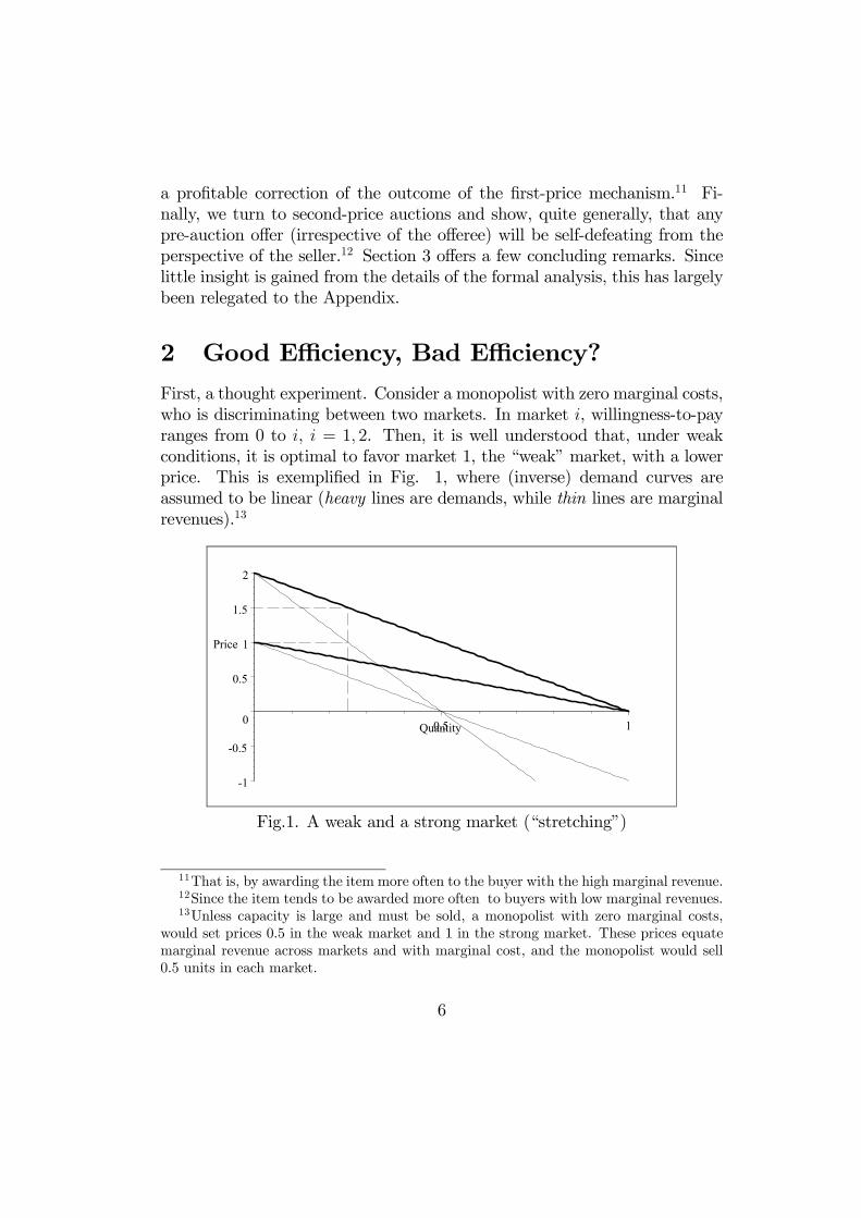
First, a thought experiment. Consider a monopolist with zero marginal costs,who is discriminating between two markets. In market i, willingness-to-payranges from 0 to i, i = 1, 2. Then, it is well understood that, under weakconditions, it is optimal to favor market 1, the “weak” market, with a lowerprice. This is exemplified in Fig. 1, where (inverse) demand curves areassumed to be linear (heavy lines are demands, while thin lines are marginalrevenues).13

-1

-0.5

0

0.5

1

1.5

2

Price

0.5 1Quantity

Fig.1. A weak and a strong market (“stretching”)

11That is, by awarding the item more often to the buyer with the high marginal revenue.12Since the item tends to be awarded more often to buyers with low marginal revenues.13Unless capacity is large and must be sold, a monopolist with zero marginal costs,

would set prices 0.5 in the weak market and 1 in the strong market. These prices equatemarginal revenue across markets and with marginal cost, and the monopolist would sell0.5 units in each market.

6

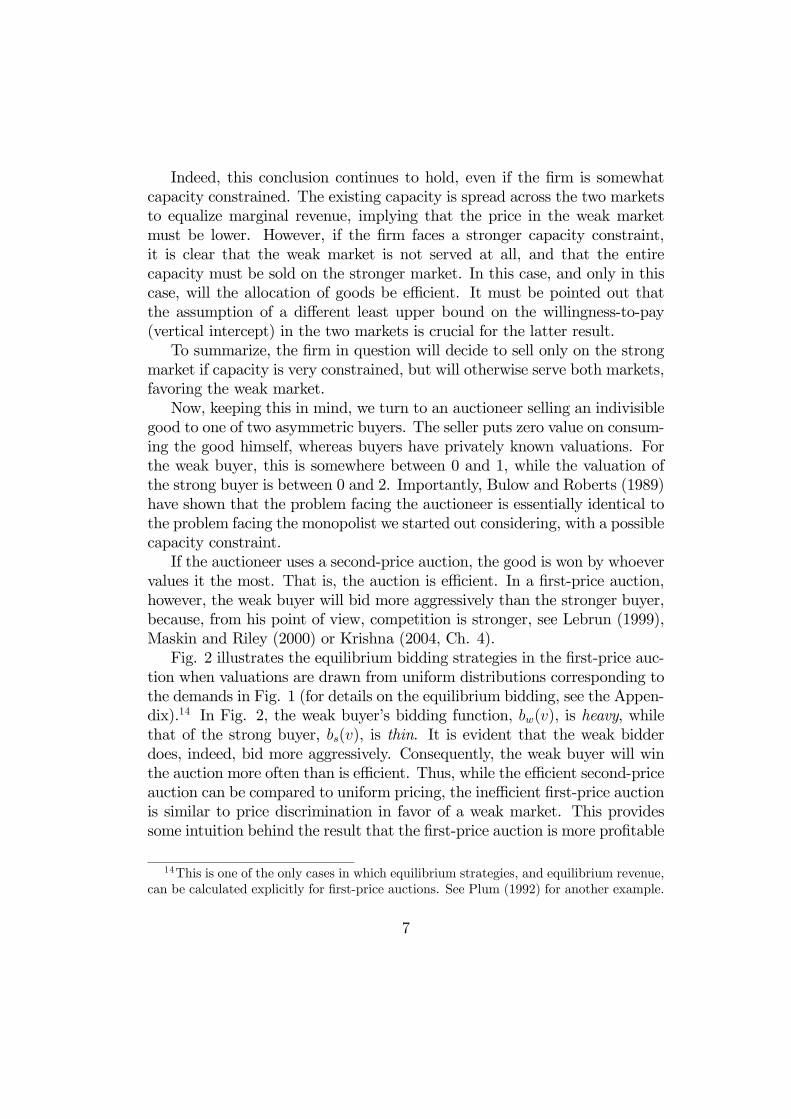
Indeed, this conclusion continues to hold, even if the firm is somewhatcapacity constrained. The existing capacity is spread across the two marketsto equalize marginal revenue, implying that the price in the weak marketmust be lower. However, if the firm faces a stronger capacity constraint,it is clear that the weak market is not served at all, and that the entirecapacity must be sold on the stronger market. In this case, and only in thiscase, will the allocation of goods be efficient. It must be pointed out thatthe assumption of a different least upper bound on the willingness-to-pay(vertical intercept) in the two markets is crucial for the latter result.To summarize, the firm in question will decide to sell only on the strong

market if capacity is very constrained, but will otherwise serve both markets,favoring the weak market.Now, keeping this in mind, we turn to an auctioneer selling an indivisible

good to one of two asymmetric buyers. The seller puts zero value on consum-ing the good himself, whereas buyers have privately known valuations. Forthe weak buyer, this is somewhere between 0 and 1, while the valuation ofthe strong buyer is between 0 and 2. Importantly, Bulow and Roberts (1989)have shown that the problem facing the auctioneer is essentially identical tothe problem facing the monopolist we started out considering, with a possiblecapacity constraint.If the auctioneer uses a second-price auction, the good is won by whoever

values it the most. That is, the auction is efficient. In a first-price auction,however, the weak buyer will bid more aggressively than the stronger buyer,because, from his point of view, competition is stronger, see Lebrun (1999),Maskin and Riley (2000) or Krishna (2004, Ch. 4).Fig. 2 illustrates the equilibrium bidding strategies in the first-price auc-

tion when valuations are drawn from uniform distributions corresponding tothe demands in Fig. 1 (for details on the equilibrium bidding, see the Appen-dix).14 In Fig. 2, the weak buyer’s bidding function, bw(v), is heavy, whilethat of the strong buyer, bs(v), is thin. It is evident that the weak bidderdoes, indeed, bid more aggressively. Consequently, the weak buyer will winthe auction more often than is efficient. Thus, while the efficient second-priceauction can be compared to uniform pricing, the inefficient first-price auctionis similar to price discrimination in favor of a weak market. This providessome intuition behind the result that the first-price auction is more profitable

14This is one of the only cases in which equilibrium strategies, and equilibrium revenue,can be calculated explicitly for first-price auctions. See Plum (1992) for another example.

7

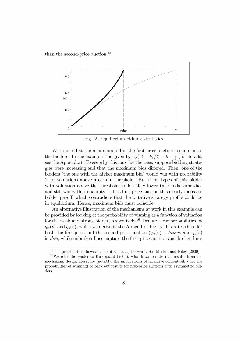
than the second-price auction.15

0

0.2

0.4

0.6

bid

1 2value

Fig. 2. Equilibrium bidding strategies

We notice that the maximum bid in the first-price auction is common tothe bidders. In the example it is given by bw(1) = bs(2) = b = 2

3(for details,

see the Appendix). To see why this must be the case, suppose bidding strate-gies were increasing and that the maximum bids differed. Then, one of thebidders (the one with the higher maximum bid) would win with probability1 for valuations above a certain threshold. But then, types of this bidderwith valuation above the threshold could safely lower their bids somewhatand still win with probability 1. In a first-price auction this clearly increasesbidder payoff, which contradicts that the putative strategy profile could bein equilibrium. Hence, maximum bids must coincide.An alternative illustration of the mechanisms at work in this example can

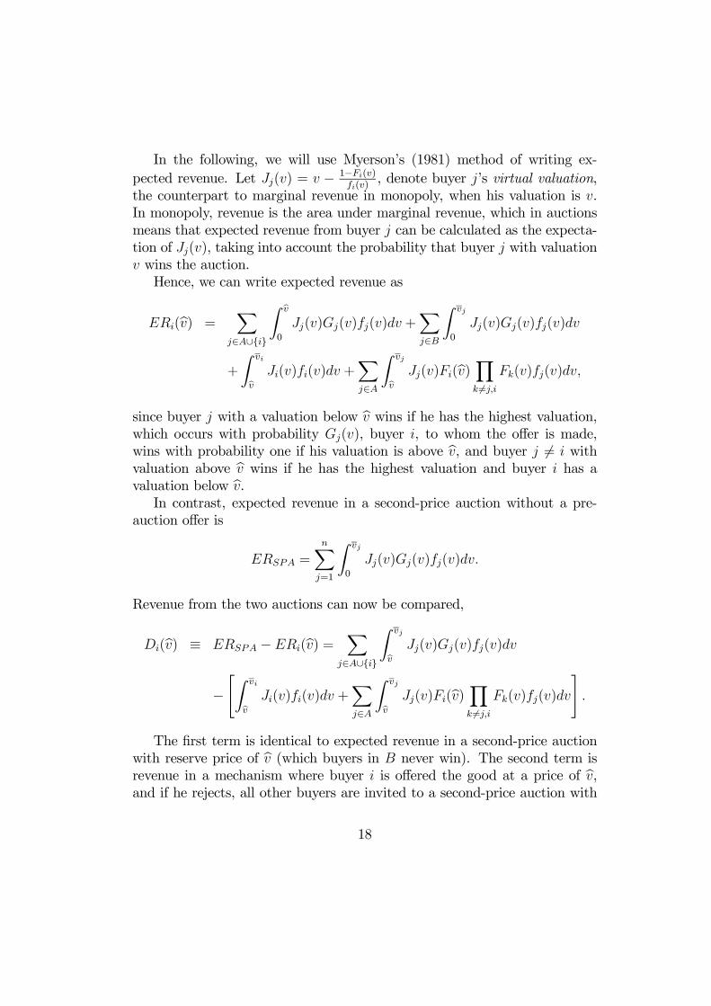
be provided by looking at the probability of winning as a function of valuationfor the weak and strong bidder, respectively.16 Denote these probabilities byqw(v) and qs(v), which we derive in the Appendix. Fig. 3 illustrates these forboth the first-price and the second-price auction (qw(v) is heavy, and qs(v)is thin, while unbroken lines capture the first-price auction and broken lines

15The proof of this, however, is not as straightforward. See Maskin and Riley (2000).16We refer the reader to Kirkegaard (2005), who draws on abstract results from the

mechanism design literature (notably, the implications of incentive compatibility for theprobabilities of winning) to back out results for first-price auctions with asymmetric bid-ders.

8

capture the second-price auction).

0

1

q(v)

1 2v

Fig. 3. Probability of winning

First, consider the first-price auction. At low valuations the strong bidderhas a higher probability of winning compared to the weak bidder, while theopposite is true at high valuations. Hence, while the weak bidder bids uni-formly more aggressively, the fact that the distribution of the strong bidderis “stretched” implies that this aggression is dominated by the strength ofthe competition at “low” valuations. In contrast, in the second-price auctionbidders bid their values, and the strong bidder has a uniformly higher prob-ability of winning, since he is facing weaker bidding competition. In otherwords, the weak buyer is “favored” in the first-price auction, while this is notthe case in the second-price auction.

2.1 Pre-auction offers in first-price auctions

Despite the remarks above, the first-price auction is not ideal from the per-spective of the auctioneer. The equilibrium in a first-price auction involvesbuyers following strictly increasing bidding strategies, ranging from zero (orthe reserve price) to a common maximal bid. That is, the strong buyer withvaluation 2 would bid the same as the weak buyer with valuation 1. Clearly,this implies that the weak buyer with valuation 1 wins more often than isefficient. Though this may appear to be beneficial for the auctioneer, the factof the matter is that, while it is profitable to favor the weak buyer, it can be

9

overdone. In Fig. 1, for example, the weak buyer should never be favored tosuch a degree that he outbids the strong buyer with a valuation above 1.5(for which marginal revenue, or virtual valuation, of the strong buyer is 1).To remedy this drawback, we propose a pre-auction offer to the strong

buyer.17 The strong buyer is given the choice of buying the good outright atthe proposed price, or to reject, in which case a first-price auction is held.The offer should be so high that it appeals to the strong buyer only if hisvaluation is high (somewhere above 1.5). This allows “efficiency at the top”— the strong buyer wins for sure if his valuation is very high — while favoringthe weak buyer when the strong buyer does not have a very high valuation.18

However, this mechanism has its weak spots as well. In particular, ifthe strong buyer rejects the pre-auction offer, the weak buyer infers thatthe strong buyer is not so strong after all. Therefore, the incentive to bidaggressively is diminished. While the weak buyer still bids more aggressivelythan the strong buyer, the difference declines. The weak buyer wins lessoften than without the pre-auction offer. Since the weak buyer is not favoredas much, this raises the possibility that revenue decreases.To examine the size of the two opposing forces on revenue by introducing

a pre-auction offer, we assume in the following that valuations are drawnfrom uniform distributions over the aforementioned ranges. While most ofthe details are in the Appendix, we outline the analysis in the following.For any given pre-auction offer, p, it is easy to show that there is a uniquethreshold equilibrium, in which the strong buyer accepts the pre-auction offerif, and only if, his valuation exceeds some valuation, z(p).19 Thus, rather thandeciding on a pre-auction offer, p, we will consider the choice of a thresholdvaluation, z, to target. The higher z is, the higher the pre-auction offer is,and the less likely it is that the offer is accepted. Fig. 4 depicts the expectedrevenue from any choice of z, z ∈ [1.5, 2]. If z = 2, the offer is never accepted,and the mechanism is essentially the unmodified first-price auction.

17As noted in the Introduction, for the type of (targeted) pre-auction offer consideredin this paper to make sense, we have to be able to identify a priori who in strong. Thus,the pre-auction offers considered in this paper are conceptually very different from thebuy-out prices analysed in, e.g., Kirkegaard & Overgaard (2004). A buy-out price is morelike a pre-auction offer made to all potential buyers in non-discriminatory fashion.

18Making a pre-auction offer to the weak buyer makes little sense, since this wouldintroduce even more severe inefficiencies at the top.

19If p is rejected, the weak buyer infers that the strong buyer’s valuation is below z. Inthe ensuing auction, the common maximal bid is exactly p.

10

0.454

0.456

0.458

1.5 2z

Fig. 4. Profit as a function of the threshold with z in [1.5, 2]

Fig. 4 reveals that the auctioneer can benefit from stipulating a pre-auction offer which is accepted with positive probability. The optimal thresh-old, z∗, is approximately 1.885, which is induced by a pre-auction price ofp∗ ' 0.653, while the probability of acceptance by the strong bidder is ap-proximately 0.058. If the pre-auction offer is rejected, the common maximalbid in the auction is p∗ ' 0.653, and Fig. 5 illustrates the bidding strategies(the dashed lines replicate the baseline case from Fig. 2 without a pre-auctionoffer to the strong bidder).

0 1v

Fig. 5. Bidding in first-price auction with and without pre-auction offer

11

With a pre-auction offer, we note that the weak buyer bids less aggres-sively in the auction after the strongest opponent types have been eliminatedby taking the offer. This captures that, for the weak buyer, competition hasbecome weaker, and it is expected to take less to win. In contrast, the re-maining, “low” types of the strong buyer bid more aggressively. To see this,recall that in a first-price format, where the winner pays his bid, any biddermust weigh the decrease in payoff from winning against the increased prob-ability of winning when the bid is raised. But here the increased density ofopponent bids (due to the compression of the weak buyer’s bidding interval)tilts this cost-benefit trade-off in favor of higher bids. Hence, the remainingtypes of the strong buyer bid more aggressively.In addition to the fact that a pre-auction offer improves revenue, it is

interesting to observe that the threshold should be strictly higher than 1.5,the point at which the strong buyer’s marginal revenue (virtual valuation)enters the range of the weak buyer’s marginal revenue from above. Thereason is that by reducing the asymmetry too much in the auction followingthe offer, the weak buyer is favored too little.

2.2 Pre-auction offers in second-price auctions

Next, we show that pre-auction offers in second-price auctions will alwaysdecrease revenue. To illustrate, we start with another thought experiment.The monopolist depicted in Fig. 1 is deciding whether to sell his entirecapacity to one particular market, rather than setting the same price in bothmarkets (uniform pricing) to clear his capacity. The former choice allowssome (extreme) discrimination betweenmarkets, whereas the latter is efficientand favors neither market. Despite this, it is easy to see that uniform pricingdominates exclusive dealing. The reason is quite simply that by combiningthe two markets into one (as under uniform pricing), willingness-to-pay fora given capacity is higher than if one deals only with one market.20 Forexample, in Fig. 1, if capacity is 0.8, the choices are to sell everything onmarket 1 at a unit price of 0.2, to sell everything on market 2 at a unitprice of 0.4, or to sell at a capacity clearing price of 0.8 across both markets.Uniform pricing is more profitable, as it yields a higher unit price.21

20Notice that this argument does not rely on one market being stronger than the other.21An alternative explanation might be useful. Assume the monopolist is initially selling

his capacity of 0.8 to market 2. By reverting to uniform pricing, and a price of 0.8, he

12

Now, as suggested already, a second-price auction can be compared touniform pricing, since no one is favored, and the buyer with the highest valu-ation wins (efficiency). Likewise, a pre-auction offer in a second-price auctionis to some extent similar to exclusive dealing in a monopoly. If the buyertargeted accepts the offer, inefficiency may result because another buyer mayhave a higher valuation. Efficiency can be restored only by abolishing thepre-auction offer and treating all buyers the same.22 As in the monopolycase, the efficient auction (without a pre-auction offer) is more profitablethan favoring one particular buyer. A formal proof of this can be found inthe Appendix. The result holds for any number of buyers, and does notrequire that one buyer is stronger than others.23 Specifically, assume thereare n risk neutral buyers. Buyer i draws a valuation independently from thedistribution Fi on [0, vi], i = 1, ..., n. Fi has no mass points, and is strictlyincreasing and continuously differentiable on (0, vi). Then we can state.

Proposition 1 A second-price auction preceded by a pre-auction offer isrevenue-dominated by the straight second-price auction.

3 Concluding Remarks

In this paper, we have considered auctions with asymmetric bidders. Then,it is well known that standard auctions are neither revenue equivalent nornecessarily efficient. Therefore, we analyzed whether pre-auction offers madeexclusively to particular bidders raise revenue, and we showed that this canbe the case when rejected offers are followed by a first-price auction, but neverwhen rejected offers are followed by a second-price auction.24 Moreover, apre-auction offer may increase efficiency in the first price auction, whereas itwill lead to a loss in efficiency in the second price auction.

will sell only 0.6 on market 2, and the remaining 0.2 on market 1. The loss on market2 is captured by the lost marginal revenue on 0.2 units. Since marginal revenue is belowdemand, this must be below 0.8 on each unit moved from market 2 to market 1. On theother hand, the gain is on average 0.8 for each of the units moved (since revenue on eachunit is 0.8). Hence, the gain exceeds the loss.

22In contrast, abolishing pre-auction offers in first-price auctions does not restore effi-ciency.

23Also, the result remains valid in the presence of a reserve price (at least one belowthe pre-auction offer). Hence, we are not constrained to looking at “must sell” auctions.

24In contrast, under standard regularity and with symmetric buyers, Bulow & Klem-perer (1996) show that pre-auction offers decrease revenue, regardless of the format.

13

ReferencesBudish, E., and L. Takeyama, 2001, Buy Prices in Online Auctions: Ir-

rationality on the Internet?, Economics Letters 73: 325-333.Bulow, J., & P. Klemperer, 1996, Auctions Versus Negotiation, American

Economic Review 86: 180-194.Bulow, J., & J. Roberts, 1989, The Simple Economics of Optimal Auc-

tions, Journal of Political Economy 97: 1060-1090.Hidvégi, Z., W.Wang and A.Whinston, 2003, Buy-Price English Auction,

forthcoming Journal of Economic Theory.Ivanova-Stenzel, R. & S. Kröger, 2005, Behavior in Combined Mecha-

nisms: Auctions with a Pre-Negotiation Stage - An Experimental Investiga-tion, Department of Economics, University of Arizona, Tucson.Kirkegaard, R., 2005, Winners and Losers in Asymmetric First Price

Auctions, Department of Economics, Brock University.Kirkegaard, R., 2006, A Short Proof of the Bulow-Klemperer Auctions

vs. Negotiations Result, Economic Theory 28: 449-452.Kirkegaard, R., & P.B. Overgaard, 2004, Buy-Out Prices in Auctions:

Seller Competition and Multi-Unit Demand, School of Economics and Man-agement, University of Aarhus.Krishna, V., 2002, Auction Theory, Academic Press, San Diego: Calif.Lebrun, B., 1999, First Price Auctions in the N Bidder Case, International

Economic Review 40: 125-142.Maskin, E., & J. Riley, 2000, Asymmetric Auctions, Review of Economic

Studies 67: 413-438.Mathews, T., 2003, A Risk Averse Seller in a Continuous Time Auction

with a Buyout Option, Brazilian Electronic Journal of Economics 5:2.Mathews, T., 2004, The Impact of Discounting on an Auction with a

Buyout Option: A Theoretical Analysis Motivated by eBay’s Buy-It-NowFeature, Journal of Economics 81: 25-52.Plum, M., 1992, Characterization and Computation of Nash-Equilibria

for Auctions with Incomplete Information, International Journal of GameTheory 20: 398-418.Reynolds, S., and J. Wooders, 2003, Auctions with a Buy Price, Depart-

ment of Economics, University of Arizona, Tucson.

14

AppendixFirst-price auctions. Assume the weak buyer’s valuation is drawn from theuniform distribution over [0, 1], while the strong buyer’s valuation is drawnfrom the uniform distribution over [0, z], z ≥ 1. Then, we know from theanalysis of Maskin and Riley (2000) or Krishna (2002) that the highest bidis

z

1 + z, (A1)

while the bidding functions are

bw(v; z) =z2

(z2 − 1)v

Ã1−

r1− (z

2 − 1)z2

v2

!, v ∈ [0, 1]

bs(v; z) =z2

(z2 − 1)v

Ãr1 +

(z2 − 1)z2

v2 − 1!, v ∈ [0, z)

where w denotes the weak buyer, and s the strong buyer.For example, when z = 2, we get bw(v) = 2

3v(2−√4− 3v2) and bs(v) =

23v(√4 + 3v2 − 2). These bidding functions are depicted in Fig. 2. Given

these, the weak buyer with valuation v outbids the strong buyer if the strongbuyer has a valuation below ev, where ev solves bw(v) = bs(ev). This event hasprobability qw(v) = v√

4−3v2 . Similarly, a strong bidder with valuation v winswith probability qs(v) = 2v√

4+3v2. These winning probabilities are graphed in

Fig. 3, alongside the winning probabilities for the buyers in a second-priceauction.25

More generally, for any z, the inverse bid functions are

vw(b) =2b

1 +¡1− 1

z2

¢b2

vs(b) =2b

1 +¡1z2− 1¢ b2 .

Then, the probability that the winning bid is below b, Fz(b), is the prob-ability that both buyers have valuations below the valuation for which a bidof b would be submitted,

Fz(b) =2b

1 +¡1− 1

z2

¢b2× 1

z

Ã2b

1 +¡1z2− 1¢ b2

!=−4γz

b2

b4 − γ(A2)

25In a second-price auction, a buyer wins whenever the rival has a lower valuation thanhimself.

15

where γ = 1

(1− 1z2)2 . Letting fz(b) be the density of the winning bid, expected

revenue in a first-price auction with the distributions under considerationwould therefore be Z b

0

bfz(b)db = b−Z b

0

Fz(b)db, (A3)

which can be computed, given (A2).We now turn to the first-price auction with a pre-auction offer. Again,

letting p denote the pre-auction offer, we claim the strong buyer acceptsp if, and only if, his valuation exceeds z, where z (uniquely) solves p =z1+z. We start by assuming the proposed strategies form an equilibrium, and

confirm this by showing that there is no incentive to deviate. First, if theauction stage is reached, the beliefs, given the strategy in the first stage, isthat buyers’ valuations are drawn from uniform distributions over [0, 1] and[0, z], respectively. Given this, the equilibrium bidding strategies are outlinedabove. If the strong buyer deviates in the first stage, rejecting p when hisvaluation was above z, it is easy to show that his best response in the firstprice auction is to submit the highest bid, z

1+z.26 Thus, regardless of whether

he accepts or rejects, he will win with probability one, and he will pay z1+z.

Hence, there is no incentive to deviate. Neither is there an incentive for thestrong buyer with a valuation below z to accept p. The reason is that he canjust submit a bid of z

1+zin the second stage and win with probability one,

so he will be no worse off rejecting.In the mechanism with a pre-auction offer, the good may be sold in the

first stage, at the price stipulated by the auctioneer, z1+z, or it may be sold in

the second stage, where bidding strategies have already been outlined, givengeneral beliefs on z. Specifically, the object is sold in the first round withprobability 2−z

2, i.e. the probability that the strong buyer has a valuation

in excess of z. With probability z2, the strong buyer rejects the offer, in

which case the weak buyer updates his beliefs, and the expected revenue willtherefore be (A3). Hence, expected revenue in the new mechanism is, as afunction of z,

26To see this, notice that the strong buyer with valuation v tries to maximize (v−b)qs(b),where qs(b) is the probability that the weak buyer bids below b. At any b where the firstderivative is zero for a v below z, it must be strictly positive for v > z.

16

ER(z) =2− z

2b+

z

2

Ãb−

Z b

0

Fz(b)db

!= b− z

2

Z b

0

Fz(b)db

= b+ 2γ

Z b

0

b2

b4 − γdb = b+ 2γ

Z b

0

b2

(b2 + γ1/2)(b− γ1/4)(b+ γ1/4)db

= b+ 2γ

Z b

0

µ1

4γ1/4 (b− γ1/4)− 1

4γ1/4 (b+ γ1/4)+1

2

1

b2 + γ1/2

¶db

= b− γ3/4

2

Z b

0

µ1

(γ1/4 − b)+

1

(b+ γ1/4)− 2γ1/4 1

b2 + γ1/2

¶db

= b− γ3/4

2

−"ln ¡γ1/4 − b¢

(b+ γ1/4)

#b0

− 2γ1/4· −1γ1/4

tan−1µγ1/4

b

¶¸b0

= b− γ3/4

2

µln

µb+ γ1/4

γ1/4 − b

¶+ 2

µtan−1

µγ1/4

b

¶− π

2

¶¶.

This function is graphed in Fig. 4.

Second-price auctions. Assume there are n risk neutral buyers. Buyer idraws a valuation independently from the distribution function Fi on [0, vi],i = 1, ..., n. Fi has no mass points, is strictly increasing and continuouslydifferentiable on (0, vi), with fi denoting the density. If v > vi, Fi(v) = 1and fi(v) = 0. Without loss of generality, the buyers are ordered such thatvn ≥ vn−1 ≥ ... ≥ v1.We consider the possibility that the seller makes a pre-auction offer to

some buyer, buyer i, say. Buyer i accepts if his valuation is at least bv. Noticethat if i = n and bv ≥ vn−1 with vn > vn−1, the pre-auction offer does notchange the allocation, as buyer n would win regardless, when his valuationexceeds vn−1. By the Revenue Equivalence Theorem, revenue is unaffected.Hence, we consider thresholds below vn−1 in the following.Let A be the set of buyers other than buyer i who are affected by the

pre-auction offer. If j ∈ A, then vj ≥ bv, meaning that there is a chance buyerj has the highest valuation, yet loses to buyer i. Let B be the set of buyersnot in A (with vj < bv) and different from i.Finally, let Gj(v) =

Yk 6=j

Fk(v), be the probability that buyer j with valu-

ation v has the highest valuation.

17

In the following, we will use Myerson’s (1981) method of writing ex-pected revenue. Let Jj(v) = v − 1−Fi(v)

fi(v), denote buyer j’s virtual valuation,

the counterpart to marginal revenue in monopoly, when his valuation is v.In monopoly, revenue is the area under marginal revenue, which in auctionsmeans that expected revenue from buyer j can be calculated as the expecta-tion of Jj(v), taking into account the probability that buyer j with valuationv wins the auction.Hence, we can write expected revenue as

ERi(bv) =X

j∈A∪{i}

Z bv0

Jj(v)Gj(v)fj(v)dv +Xj∈B

Z vj

0

Jj(v)Gj(v)fj(v)dv

+

Z vi

bv Ji(v)fi(v)dv +Xj∈A

Z vj

bv Jj(v)Fi(bv)Yk 6=j,i

Fk(v)fj(v)dv,

since buyer j with a valuation below bv wins if he has the highest valuation,which occurs with probability Gj(v), buyer i, to whom the offer is made,wins with probability one if his valuation is above bv, and buyer j 6= i withvaluation above bv wins if he has the highest valuation and buyer i has avaluation below bv.In contrast, expected revenue in a second-price auction without a pre-

auction offer is

ERSPA =nX

j=1

Z vj

0

Jj(v)Gj(v)fj(v)dv.

Revenue from the two auctions can now be compared,

Di(bv) ≡ ERSPA − ERi(bv) = Xj∈A∪{i}

Z vj

bv Jj(v)Gj(v)fj(v)dv

−"Z vi

bv Ji(v)fi(v)dv +Xj∈A

Z vj

bv Jj(v)Fi(bv)Yk 6=j,i

Fk(v)fj(v)dv

#.

The first term is identical to expected revenue in a second-price auctionwith reserve price of bv (which buyers in B never win). The second term isrevenue in a mechanism where buyer i is offered the good at a price of bv,and if he rejects, all other buyers are invited to a second-price auction with

18

a reserve price of bv. Clearly, the former auction is more profitable, implyingthat Di(bv) > 0 as we wanted to prove.An alternative proof starts by examining the derivative of ERi(bv),ERi

0(bv) = fi(bv)"Xj∈A

Z vj

bv Jj(v)Yk 6=j,i

Fk(v)fj(v)dv − Ji(bv)(1−Gi(bv))# .The first term in brackets is equivalent to the expected revenue in a second-price auction with a reserve price of bv among all the buyers except buyeri. This clearly exceeds revenue from posting a price of bv, which would yieldexpected revenue of bv(1−Gi(bv)). Hence,

ERi0(bv) ≥ fi(bv)(1−Gi(bv))(bv − Ji(bv)) = (1−Gi(bv))(1− Fi(bv)) ≥ 0.

It follows that a pre-auction offer never improves revenue in a second-priceauction.27 Notice that we have not assumed that Jj is monotonic, as isoften the case in auction theory. Bulow and Klemperer (1996) argued thatpre-auction offers are not profitable in a model with symmetric buyers andmonotonic virtual valuations. Hence, we generalize this result in severaldirections.To reveal the intuition behind the result we rearrange the derivative,

ERi0(bv) = fi(bv)(1−Gi(bv))"X

j∈A

Z vj

bv Jj(v)Yk 6=j,i

Fk(v)fj(v)

(1−Gi(bv))dv − Ji(bv)# .If the pre-auction offer changes the allocation, it is because buyer i winswhen another buyer (in A) has a higher valuation. In this event, the gaincontributing to an increase in revenue is the virtual valuation of buyer i,Ji(bv) ≤ bv. The loss, however, is the virtual valuation of a buyer known tohave a higher valuation. This is at least equal to bv. On a market wherethe lowest willingness-to-pay is bv a monopolist can get at least bv for each ofhis units (and strictly more if he faces a capacity constraint), so the averagemarginal revenue, or virtual valuation, is at least bv. Hence, the loss fromintroducing a pre-auction offer exceeds the gain.

27Clearly, for any i, A and B depend on bv. Given A and B, however, revenue increasesby increasing bv until buyers move from A to B (bv = minj∈A vj). As we reduce A further,revenue increases. For any given i, it follows that the optimal bv = vi, which is equivalentto no pre-auction offer.

19

Working Paper

2005-5: Niels Haldrup, Peter Møllgaard and Claus Kastberg Nielsen:Sequential versus simultaneous market delineation: The relevantantitrust market for salmon

2005-6: Charlotte Christiansen, Juanna Schröter Joensen and JesperRangvid: Do More Economists Hold Stocks?

2005-7: Ott Toomet: Does an increase in unemployment income lead tolonger unemployment spells? Evidence using Danish unemploy-ment assistance data.

2005-8: Marianne Simonsen: Availability and Price of High Quality DayCare and Female Employment.

2005-9: Francesco Busato, Bruno Chiarini and Enrico Marchetti: FiscalPolicy under Indeterminacy and Tax Evasion.

2005-10: Francesco Busato, Bruno Chiarini, Pasquale de Angelis and Eli-sabetta Marzano: Capital Subsidies and the Underground Econ-omy.

2005-11: Francesco Busato, Alessandro Girardi and Amedeo Argentiero:Do sector-specific shocks explain aggregate fluctuations.

2005-12: Hristos Doucouliagos and Martin Paldam: Aid Effectiveness onAccumulation. A Meta Study.

2005-13: Hristos Doucouliagos and Martin Paldam: Aid Effectiveness onGrowth. A Meta Study.

2005-14: Hristos Doucouliagos and Martin Paldam: Conditional Aid Ef-fectiveness. A Meta Study.

2005-15: Hristos Doucouliagos and Martin Paldam: The Aid EffectivenessLiterature. The Sad Result of 40 Years of Research.

2005-16: Tryggvi Thor Herbertsson and Martin Paldam: Does Develop-ment Aid Help Poor Countries Catch Up? An Analysis of theBasic Relations.

2005-17: René Kirkegaard and Per Baltzer Overgaard: Pre-Auction Offersin Asymmetric - First-Price and Second-Price Auctions.