AD-AD92 636 STANFORD UNIV CA DEPT OF STATISTICS F/6 12/1COCHRAN'S THEOREM, RANK ADDITIVITY, AND TRIPOTENT MATRICES.(U)AUG 80 T W ANDERSON, 6 P STYAN N0001-75-C-0442

UNCLASSIFIED TR-43 NL

E 'llmmmmmmmlEIEEEIIIEIIII-IIIIIIIEI-

W11 111-II 1112.2

70 1111-0

1111J2 _L4 mA

11111 11 1111.

MICROCOPY RESOLUTION TEST CHART

NATIONAL BUREAU OF SIANDARDS %qh3 A

_--..

z LEVkQCOCHRAN'S THEOREM, RANK ADDITIVITY,

AND TRIPOTENT MATRICES

BY

T. W. ANDERSON and GEORGE P. H. STYAN

TECHNICAL REPORT NO. 43AUGUST 1980

PREPARED UNDER CONTRACT N00014-75-C-0442

(NR-042-034)

OFFICE OF NAVAL RESEARCH

THEODORE W. ANDERSON, PROJECT DIRECTOR

DTICSELECTE,DEC 9 1980

DEPARTMENT OF STATISTICSB

STANFORD UNIVERSITY

STANFORD, CALIFORNIA

CDS STATEMENT

Approved for public release;LI Distribution Unlimited

__s _ 80 '2 03 OiljV,- 4

COCHRAN'S THEOREM, RANK ADDITIVITY,

AND TRIPOTENT MATRICES

by

T. W. AndersonStanford University

and

George P. H. StyanMcGill University

TECHNICAL REPORT NO. 43

AUGUST 1980

PREPARED UNDER CONTRACT NOOo1-75-C-04h2(NR-o42-034)

OFFICE OF NAVAL RESEARCH

Theodore W. Anderson, Project Director

Reproduction in Whole or in Part is Permitted forany Purpose of the United States Government

Approved for public release; distribution unlimited.

DEPARTMENT OF STATISTICSSTANFORD UNIVERSITYSTANFORD, CALIFORNIA

Cochran's Theorem, Rank Additivity,

and Tripotent Matrices

T. W. Anderson and George P. H. Styan

Stanford University and McGill University

1. Introduction

Let x be a pxl random vector distributed according to a multivariate

normal distribution with mean vector 0 and covariance matrix I . We will-p

denote this by x A N(O, I p). Let ql .... qk be quadratic forms in x with

ranks rI , ... rk, respectively, and suppose that Jqi = x x. Then what

has become well known as Cochran's Theorem is Theorem II of Cochran

(193h, p. 179): A necessary and sufficient condition that q., ... qk

be independently distributed as X is that Jri P.

Rao (1973, §3b.h) gives this result with x - N(p, I) as the Fisher-

Cochran Theorem. Fisher (1925) showed that if the quadratic form q in x

2 ,' 2 ineedtlis distributed as Xh then x x - q is distributed as Xph independently

of q, cf. James (1952).

Our purpose in this paper is to review various extensions of

Cochran's Theorem in a bibliographic and historical perspective, with

special emphasis on matrix-'heoretic analogues. While we present, over

30 references, we note that Scarowsky (1973) has a rather complete

discussion and bibliography on the distribution of quadratic forms in

k ,.oIJ

normal random variables. See also the bibliography by Anderson, Das

Gupta, and Styan (1972), where 90 research papers published through 1966

are listed under subject-matter code 2.5 (distribution of quadratic and

bilinear forms in normal variables).

The first section is devoted to a survey of results summarized in

Theorems 1.1 and 1.2. The proofs are given in Section 2. In the

following section the extensions from idempotent to tripotent matrices i!

are given and proved.

To formulate our first matrix-theoretic extension of Cochran's

Theorem we let AI ..... A k be pxp symmetric matrices and write A =A

Consider the following statements:

2(a) A = Ai i ..

(b) AiAj = 0 for all iWJ,

(c) A = 1,

(d) I rank(A ) = rank(A).

Then the matrix-theoretic analogue of Cochran's Theorem is:

(a), (b), (c) + (d), (1.1)

(c), (d) - (a), (b). (1.2)

The reason that these two versions of Cochran's Theorem are equivalent

follows from the following two well-known results:

2

,Si

.. . - I%

LE A 1.1. Let x -N(j, Z), with E positive definite, and let A be

262 2nonrandom and symmetric. Then x'Ax X a noncentral X distribution

2with f degrees of freedom and noncentrality parameter 6 , if and only if

2=AZA = A, and then f = trA = rank(A) and 6 p I'Ap.

We write trA for the trace of A and note that when A = A2 then

trA = rank(A); this result holds even when A is not symmetric (cf., e.g.,

Rao (1973), p. 28).

2When Z = I the condition in Lemma 1.1 reduces to A = A, and this

was first given by Craig (1943) with p = 0 and then by Carpenter (1950)

with p~ possibly nonzero. (Thus (a) is equivalent to qi = x'A.x having

aX2 distribution with number of degrees of freedom equal to rank(A.).)

Sakamoto (1944, Th. II, p. 5) gave the more general version, with E

positive definite and p = 0. Cochran (1934, Corollary 1, p. 179) took

x- N(O, I) and gave Lemma 1.1 with the condition that all the nonzero

eigenvalues of A be equal to 1 instead of the condition A2 = A.

LEMMA 1.2. Let x and A be defined as in Lemma 1.1 and let B be

nonrandom and symmetric. Then x'Ax and x'Bx are independently distributed

if and only if AEB = 0.

When E = I the condition in Lemma 1.2 reduces to AB = 0, and this

was first given by Craig (1943) with p = 0 and then by Carpenter (1950)

with u possibly nonzero. Again Sakamoto (1944, Th. I, p. 5) gave the

more general version with Z positive definite and Uj = 0. Their proofs,

however, turned out to be incorrect and the first correct proof of L_

Lemma 1.2 (with p = 0) seems to be by Ogawa (1948; 1949, cf. p. 85).

Cochran (1934, Theorem III, p. 181) let x - N(O, I) and gave the

condition in Lemma 1.2 as . ed

-.. Vflij/Oi

3 L .pucia

LA

I- isAI - itBI = II- isA - itBi (1.3)

for all real s and t, where i = v and 1"1 denotes determinant.

Ogasawara and Takahashi (1951, Lemma 1) gave a short proof that (1.3)

implies AB = 0 when the symmetric matrice A and B are not necessarily

positive semi-definite.

Cochran's Theorem was first extended to x - N(p , I ) by Madow (1940)-p

and then to x - N(O, E), Z positive definite, by Ogawa (1946, 1947), who

2also relaxed the condition (c) to A = A. Ogasawara and Takahashi (1951)

extended Cochran's Theorem to x - N(p, E), E positive definite, and to

x - N(O, E), with E possibly singular. Extensions to x - N(V, E), with

E possibly singular, have been given by Styan (1970, Theorem 6) and Tan

(1977, Theorem 4.2); Ogasawara and Takahashi (1951) extended Lemmas 1.1

and 1.2 to x - N(V, E), with E possibly singular.

James (1952) appears to be the first to notice that (1.1) could

be extended to

(a), (c) ( (b), (d),

(b), (c) ( (a), (d),

while

2(a), (b) A = A and (d)

follows at once from the definition of the X -distribution.

Chipman and Rao (1964) and Khatri (1968) extended the matrix

analogue of Cochran's Theorem to square matrices which are not necessarily

symmetric:

'4

I

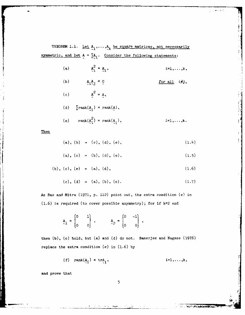
THEOREM 1.1. Let Al ... ,Ak be square matrices, not necessarily

symmetric, and let A = Ai. Consider the following statements:

2(a) A A., i=l,. .. ,k,

-1 -

(b) Aij =O for all i$J,

2(c) A A,

(d) Irank(Ai) = rank(A),

(e) rank(A ) = rank(Ai), i=l, .. ,k.

Then

(a), (b) (c), (d), (e), (1.h)

(a), (c) (b), (d), (e), (1.5)

(b), (c), (e) + (a), (d), (1.6)

(c), (d) (a), (b), (e). (1.7)

As Rao and Mitra (1971, P. 112) point out, the extra condition (e) in

(1.6) is required (to cover possible asymmetry); for if k=2 and

0 1= A 2= 0 1

then (b), (c) hold, but (a) and (d) do not. Banerjee and Nagase (1976)

replace the extra condition (e) in (1.6) by

(f) rank(A1 ) = trAi, i=l,...k,

and prove that

5

(b), (c), (f) - (a), (d); . )

however, the condition (b) is now no longer required on the left of

(1.8) since

(c), (f) (a), (b), (d)

follows from

rank(A) trA = trjA. =trAi .rank(A.)

and (1.7).

In Section 2 we present several proofs of Theorem 1.1.

Marsaglia and Styan (1974) extended Theorem 1.1 by considering an

arbitrary sum of matrices, which may now be rectangular. The analogue of

Theorem 1.1 is

THEOREM 1.2. Let AI ,.... Ak be pxq matrices, and let A = JAi •

Consider the following statements:

(a') A.A-A = Ail....k,

(b') AiA-A = 0 for all i#j,

(c') rank(AiA-Ai ) = rank(Ai),

(d') Yrank(Ai) = rank(A),

where A is some g-inverse of A. Then

(a') * (b'), (c'), (d'), (1.9)

(b'), (0') (a'), (d'), (1.10)

(d') (W'), (b'), (c'). (~ i

6

.. . - i. " h .. '.

If (a') or if (b') and (c') hold for some g-inverse A- then (a'), (b')

and (c') hold for every g-inverse A-.

In Theorem 1.2 we define a g-inverse of A as any solution A to

AAA = A, cf. Rao (1962), Rao and Mitra (1971).

The condition (c') in Theorem 1.2 plays the role of condition (e)

in Theorem 1.1.

Marsaglia and Styan (1974, Th. 13) proved (1.11), while Hartwig

(1980) has established (1.9). The proposition (1.10), however, appears

to be new and is proved in Section 2, where we also present several

different proofs of (1.7). In Section 3 we extend Theorem 1.1 to

tripotent matrices, following the work by Luther (1965), Tan (1975, 1976)

and Khatri (1977). In Section 4 we discuss the applications of these

algebraic theorems to statistics.

2. Some Proofs

2.1. Proof of Theorem 1.1. To prove (1.7) in Theorem 1.1 we begin

by reducing condition (c) to a sum being I as in the earlier version of

Cochran's Theorem; then (1.7) reduces to (1.2). We may do this since

if A is pxp, not necessarily symmetric, then, as we shall show,

2A = A 4-+ rank(I - A) = p - rank(A). (2.1)

(Note Fisher's 1925 result goes both ways, cf. Section 1, paragraph 2.)

To prove (2.1) let A 2 = A; then (I -A) 2 = I - A and so

rank(I - A) = ) = p -trA p rank(A).

7

To go the other way we follow Krafft (1978, pp. 407-408) by noting that

1(A) c C(I - A), (2.2)

where U(A) = {x :Ax = 01 is the null space of A and C(I - A) = {(I -A)xl

is the column space of I-A. (If x E)(A), then Ax = 0 and (I-A)x =

xEC(I-A).) If rank(I-A) = p - rank(A), then equality must hold in

A2(2.2) and so A= A.

We now write A I-A, and in view of (2.1) we replace (c) by

Xp Ai = I, and (d) by k= rank(A.) =p.i 0-ii 0 -i

The proof of (1.7) by Cochran (1934, p. 180), cf. also Anderson

(1958, p. 164) and Rao (1973, §3b.4), requires that Al ... 1Ak be symmetric.

In this event we may write

A. = P'P! -Q.i !i i=0,1,...,k, (2.3)

where P. is pxpi, Q. is pxqi, and A. has p. positive and q. negative

eigenvalues, cf. e.g., Anderson (1958, p. 346). In (2.3) we assume

that P. has rank p , has rank q,, and p. + qi = ri, the rank of A..

Hence

k k k

Pi=0 0 i X '- 9ii=0ii=0

-p-q q

= PJP',

say, where q = i=O qi, since from (d) now p = ri = (= Pi+q) =

(= p) + q. But (2.4) is positive definite and P is nonsingular;

8

hence q=0 and J=I. Thus qo = . =q 0 and (2.4) reduces to

Ip = (P0 ... PI :pp

and so P = (PO ... P) is an orthogonal matrix. Hence A. P P.iP.P! =k~ iI1 i

P.P! = A. since P!P. and A A = P'P P' 0 for all iiJ since-1-i -1 - - 1 -iJ- ~l~~j~J -

then P.P = 0.i-j -

We now present three other proofs of (1.7); these three proofs do

not require that AC0t... ,Ak be symmetric.

Following Craig (1938, p. 49), cf. also Aitken (1950, §6) and Rao

and Mitra (1971, pp. 111-112), we may prove (1.7) using a rank-subadditivity

argument. From (2.1) with Ak replacing A we have

p - rank(Ak) < rank(I-Ak)

-rank(A0 + + Akl)

<rank(A) + " + rank(A-0 -k-1

p - rank(Ak) (2.5)

when (d) holds. This inequality string, therefore, collapses, and

rank(I -Ak) = .ank(Ak), which implies 2k = Ak by (2.1); repeating

the argument with Ak-l' Ak_2',.. yields (a). To see that this implies

(b) we follow Rao and Mitra (1971, p. 112) by noting that the argument

used in (2.5) implies that

(Ai + A) 2 = i + A

and so

AA~ + AA =

9

----~'.

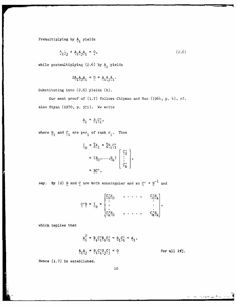
Premultiplying by Ai yields

PA +AAA =0, (2.6)

.i-i -ii = 2

while postmultiplying (2.6) by Ai yields

2Ai-J-i = 9 = -i-Ji"i

Substituting into (2.6) yields (b).

Our next proof of (1.7) follows Chipman and Rao (1964, p. 4), cf.

also Styan (1970, p. 571). We write

A. =B

where B. and C. are pxr. of rank r.. Then~I -i 1 1

Ip = A. = BC

= BC',

~-l

say. By (d) B and C are both nonsingular and so C' = B- and

C'B I'

-00 ' *' -0kC'B1 =

-k-0 9kk

which implies that

2A. B'B C' = B = Ai

AA Bfor all iiJ.

Hi-c -i-i-7 ii -

Hence (1.7) is established.

10

6 J ' i

Our last proof of (1.7) follows Loynes (1966), cf. also Searle

(1971, p. 63). A rank-subadditivity argument is used similar to that

used in (2.5):

p - rank(Ak) < rank(Ip-A)

- rank(A 0 ,A 1 ... Ak_,I p - k)

:ran(A0,...,4_I,I-A - ... -l _-Ak

- rank(Ao k-)

< rank(A ) + ... + rank(Ak_l)

- p - rank(A k).

The rest of Theorem 1.1 is easily proved. To prove (1.4) we see

that (a), (b)

A2 (y) 2 A +. A A =A+ =IA,i~j

while

I rank(A) trA. = tr A1 tr A = rank(A), (2.7)

and so (1.4) is established.

To prove (1.5) we see that (a), (c) (d) from (2.7) and so (1.5)

follows from (1.7).

To prove (1.6) we see that (b), (c)

A2 = (IAi)2 1 2 + m AiAj = 2 = =~ i~J

multiplying through by Ai yields

11

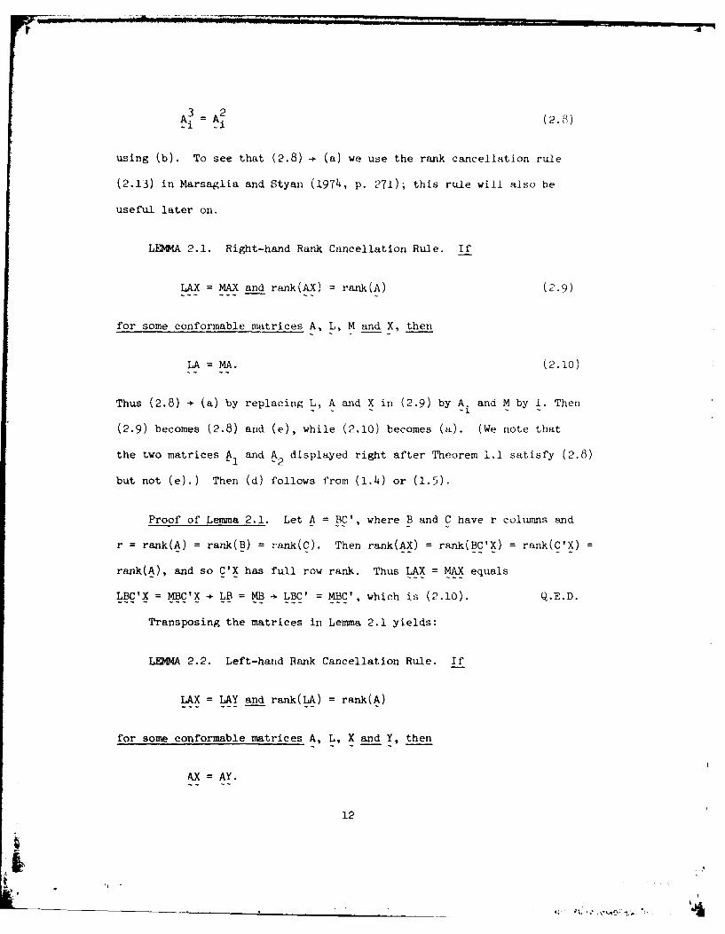
A3 A2A3 = A2 (2.S)

using (b). To see that (2.8) (a) we use the rank cancellation rule

(2.13) in Marsaglia and Styan (197h, p. 271); this rule will also be

useful later on.

LEMMA 2.1. Right-hand Rank Cancellation Rule. If

LAX = MAX and rank(AX) = rank(A) (2.9)

for some conformable matrices A, L, M and X, then

LA = (2.10)

Thus (2.8) -+ (a) by replacing L, A and X in (2.9) by A. and M by I. Then

(2.9) becomes (2.8) and (e), while (2.10) becomes (a). (We note that

the two matrices A1 and A2 displayed right after Theorem 1.1 satisfy (2.8)

but not (e).) Then (d) follows from (1.4) or (1.5).

Proof of Lemma 2.1. Let A = BC', where B and C have r columns and

r = rank(A) = rank(B) = rank(C). Then rank(AX) = rank(BC'X) rank(C'X) =

rank(A), and so C'X has full row rank. Thus LAX = MAX equals

LBC'X = MBC'X + LB = MB - LBC' = MBC', which is (2.10). Q.E.D.

Transposing the matrices in Lemma 2.1 yields:

LEMMA 2.2. Left-hand Rank Cancellation Rule. If

LAX = LAY and rank(LA) = rank(A)

for some conformable matrices A, L, X and Y, then

AX = AY.

12

tXI

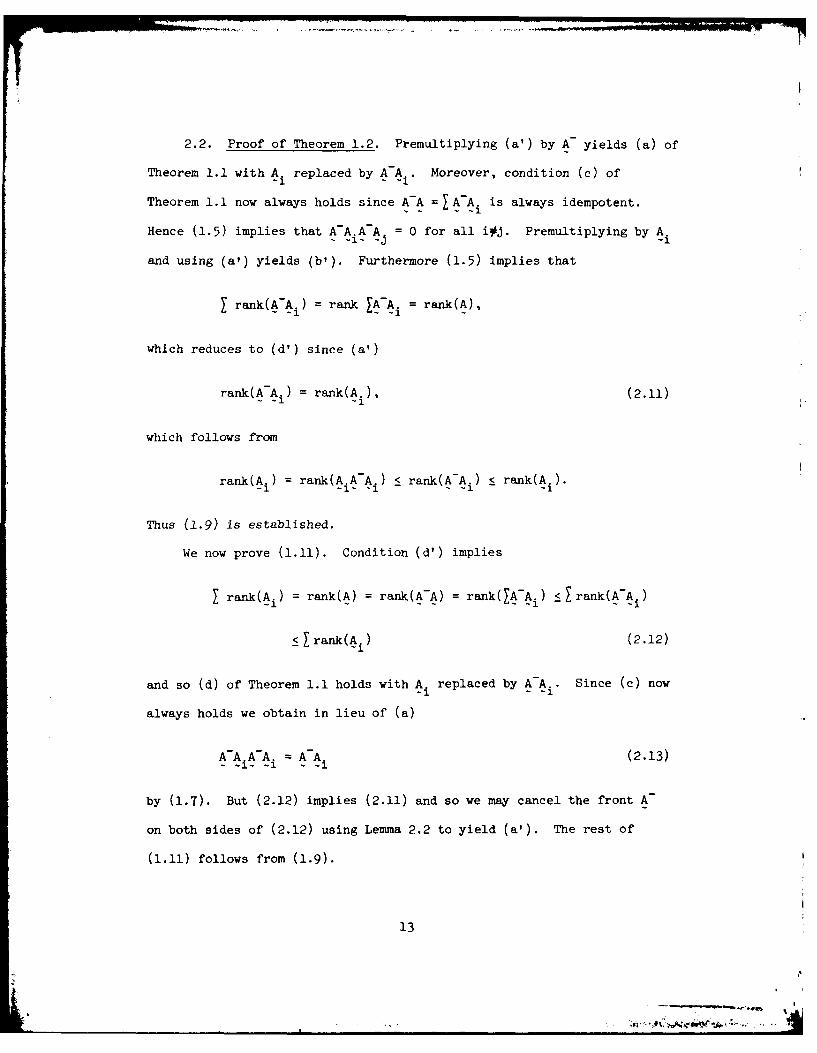
2.2. Proof of Theorem 1.2. Premultiplying (a') by A- yields (a) of

Theorem 1.1 with A.i replaced by A-A. Moreover, condition (c) of

Theorem 1.1 now always holds since A-A =1 A-A. is always idempotent.

Hence (1.5) implies that A-AiAA = 0 for all i#j. Premultiplying by A.

and using (a') yields (b'). Furthermore (1.5) implies that

rank(A- A. rank XA-A rank

which reduces to (d') since (a')

rank(A-A.) = rank(A.), (2.11)

which follows from

rank(A i) rank(AiA-A) _ rank(A-A) _ rank(Ai).

Thus (1.9) is established.

We now prove (1.11). Condition (d') implies

[ rank(Ai) = rank(A) = rank(A-A) = rank(jA-Ai ) < rank(A-A.)

_ rank(Ai) (2.12)

and so (d) of Theorem 1.1 holds with A. replaced by AA.. Since (c) now-3. - -1

always holds we obtain in lieu of (a)

A-AA-A - A-A (2.13)

by (1.7). But (2.12) implies (2.11) and so we may cancel the front A-

on both sides of (2.12) using Lemma 2.2 to yield (a'). The rest of

(1.11) follows from (1.9).

13

• i iin i i i

To prove (1.10) we use the same technique which we used above

to yield

A-A.AAAA AAiAA i, (2.14)

which is (2.8) with Ai replaced by A-A. The rank condition (c') and

Lemma 2.1 allow us to cancel the A A. on the right of both sides of (2.14)

to yield

A-A.A-A. A A. (2.15)- -i ~- -i -1~

Using (2.11) and Lemma 2.2 allows us to cancel the leading A on both

sides of (2.15) and this yields (a'). The rest of (1.10) follows from

(1.9) and the proof is complete. Q.E.D.

We may extend Theorem 1.1 to tripotent matrices using Theorem 1.2.

We do this in the next section.

3. Tripotent Matrices

A square matrix A is said to be tripotent whenever A3 = A. Tripotent

matrices have been studied by Luther (1965), Tan (1975, 1976) and

Khatri (1977). These authors considered extending Theorem 1.1 to

AI,...,A k tripotent. This is of interest in statistics since if x-N(O, I)

and A is symmetric nonrandom then x'Ax is distributed as the difference

of two independently distributed X -variates if and only if A3 A, cf.

Graybill (1969, p. 352), Tan (1975, Theorem 3.5).

114

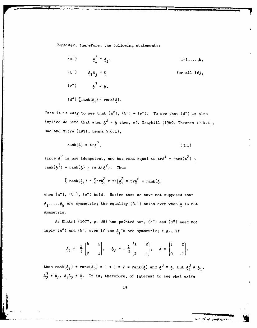
Consider, therefore, the following statements:

(a") A 3 = Ai i=l... ,k,-i

(b") AiA j =0 for all i J,

(c") A 3 = A,

(d") Irank(Ai)= rank(A).

Then it is easy to see that (a"), (b") - (c"). To see that (d") is also

implied we note that when A = A then, cf. Graybill (1969, Theorem 12.4.4),

Rao and Mitra (1971, Lemma 5.6.1),

rank(A) = trA , (3.1)

since A2 is now idempotent, and has rank equal to trA2 rank(A ) >

rank(A 3 ) = rank(A) > rank(A 2). Thus

[rank(A ) =jtrA 2 =trl 2 = trA 2 = rank(A)

when (a"), (b"), (c") hold. Notice that we have not supposed that

AI,... SAk are symmetric; the equality (3.1) holds even when A is not

symmetric.

As Khatri (1977, p. 88) has pointed out, (c") and (d") need not

imply (a") and (b") even if the Ai's are symmetric; e.g., if

1 - 21 1- 2, A =1 01l 3 2 1 2 = 3 2 40

then rank(A1 ) + rank(A2 ) =1 + 1 = 2 = rank(A) and A3 = A, but A3 0 A1 ,

-3 -2' YA2 0 0. It is, therefore, of interest to see what extra

15

-- I -'' _._

condition could be added to (c") and (d") so as to imply (a") and (b").

Khatri (1977, Lemma 10) uses

rank(A) = D{rank[Ai(A 2 +A)] + rank[Ai(A 2 -A)]), (3.2)

which is rather complicated. We may simplify (3.2) in various ways. To

do this we first note that

3-A =A +- A = , (3.3)

cf. Graybill (1969, Theorem 12.4.1), Rao and Mitra (1971, Lemma 5.6.2).

Thus Theorem 1.2 implies that (c"), (d") are equivalent to

A =i A., i1,. ... k, (..)

and

AyAj = 0 for all i#j. (3.5)

Summing (3.') over all J#i and adding to (3.4) yields

0iA = Ai, i=i,... ,k. (3.6)

Hence under (c") and (d") the condition (3.2) is equivalent to

rank(A) =3 {rank[A (I +A)I + rank[A.(I -A)f), (3.7)

which is a little simpler than (3.2). But (3.7) implies

rank(A) > 1rank(A 1 ) rank(A1 ) ( .8)

= rank(A)

when (d") holds. Thus equality holds throughout (1.8) and so (3.7) implies

rank(A1 ) = rank[A i(I +A)I + rank[A (I-A)), iI,....k. (3.9)

Summing (3.9) and using (d") yields (i.1).

16

Some motivation for the condition (3.9), and hence also for the

equivalent conditions (3.2) and (3.7), may be obtained from the following

characterization of a tripotent matrix, extending Lemma 5.6.6 in Rao and

Mitra (1971, p. 114):

LEMMA 3.1. Let A be a square matrix, not necesserily symmetric.

Then A3 = A if and only if

rank(A) = rank(A+A 2) + rank(A-A 2). (3.10)

2 2Proof. We use Theorem 1.2 with A A + A , A2 = A - A, and

A + A = 2A. If A3 = A then 1 = (2A)- and (3.10) follows from (1.9)-1 -2 = 2 - 2-

since

2 1 2 1 3 14 1 5(A+A ) A(A+A)= -A ~A +

2-

=A+A2

and similarly

(A-A) =A(A-A) A A- A

To go the other way we use (1.11). Then (3.10) implies

0 = (A + A2(A-A)13

3and so A = A and the proof is complete. Q.E.D.

This suggests using the condition

A= A2 i=l,.. ,k, (3.11)

instead of (3.9), or (3.7) or (3.2). We obtain:

17

; b .. .. . . . . . ..I

THEOREM 3.1. Let A1,... ,Ak be square matrices, not necessarily

symmetric, and let A = XAi. Then

(a") A3 = A i,-i

and

(b") AiA j = 0 for all i#j,

hold if and only if

(c") A3 - A,

(d") Yrank(Ai) = rank(A),

and

(e A.A A, i=l,...,k.-1e -"

The condition (e") may be replaced by (3.9), b (3.7), by (3.2), by

(el) A2A - A. i=l,...k,

or by

(e2) AOA - A i~l,.....k.

Proof. We have already shown that (a"), (b") imply (c"), (d") and

hence also (e"), (3.9), (3.7), (3.2), (el) and (e2). To go the other way

let (c"), (d") hold. Then (3.4) and (3.5) are true. Substituting (e")

yields (a") and A = 0 for all i#j; premultiplying by A. yields (b").

We have shown that when (c"), (d") hold, then (3.9), (3.7) and (3.2) are

equivalent. To see that (a"), (b") are implied we use Theorem 1.2 with

the A i's replaced by the Ai(I+A) and the Ai(I-A) in (3.7), which

equation shows them to be rank-additive (the sum is 2A). Then(.l1l)

implies that

18

___ ___ ___ ___~

A.(I +A)(-:A)A (I -A) =0, (312)

1 -1 - - -2-1 - - 1

using A (2A)-. Substituting (3.4) and (3.6) into (3.12) yields

(A. +A2)(I-A) - 0.-1 - - -

Postmultiplying by Aj (J#i) and using (3.5) gives

AA -A2Aj. (3.13)

However, (1.11) also implies, cf. (3.12),

A. (I- ( )A)A.(I +A) = 9,

which leads to

AA A.A . (3.14)

Adding (3.13) and (3.14) yields (b"), and substituting (b") into (3.4)

gives (a").

Now let (c"), (d"), (el) hold. Then (3.4), (3.5) hold and premulti-

plying (3.5) by A i yields (b"). Then (3.4) implies (a"). Finally, we let

(c") (d") (e2) hold. Then substitution of (e2) into (3.4) yields (el),

and the proof is complete. Q.E.D.

Khatri (1977, Lemma 10) proved the part of Theorem 3.1 with (e")

replaced by (3.2). He also claimed that (b"), (c") - (a"), (d"), (e").

But this is not so for the same reason that this does not hold in

Theorem 1.1; again if we let

A 1 11' A2 - , (3.15)

19P4

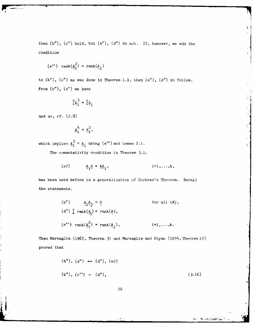
then (b"), (c") hold, but (a"), (d") do not. If, however, we add the

condition

(e"') rank(A-') = rank(A.)

to (b"), (c") as was done in Theorem 1.1, then (a"), (d") do follow.

From (b"), (c") we have

and so, cf. (2.8)

h4 2A. = Ai1 ,i

which implies A3 = A. using (e"')and Lemma 2.1.i -

The commutativity condition in Theorem 3.1:

(e2) A.A = AA.,

has been used before in a generalization of Cochran's Theorem. Recall

the statements.

(b") AA j = 0 for all i#j,

(d") I rank(Ai) = rank(A),

(e"') rank(A2 ) = rank(Ai), i=l,...,k.

Then Marsaglia (1967, Theorem 3) and Marsaglia and Styan (1974, Theorem15)

proved that

(b"), (d") +-+ (d"), (e2)

(b"), (e"') + (d"), (3.16)

20

-

while Luther (1965, Theorem 1, p. 684) and Taussky (1966, Theorem 2),

assuming the A 's to be symmetric, proved that-1

(b") -- (d"), (e2).

The condition (e"')in (3.16) cannot be dropped in view of the example

(3.15); when the Ai's are symmetric, however, (e"') is automatically

satisfied.

Luther (1965, Theorem 3, p. 689) and Tan (1976, Theorem 2.2) have

given versions of Theorem 3.1 when the A. 's are symmetric. We obtain:

THEOREM 3.2. Let A1 ,... ,Ak be symmetric matrices and let A IA.

Then

(a") A3 -Ail~ .. k

and

(b") AiAi 0 for all i#j

hold if and only if

(c") A3 A,

k(d") [ rank(A i) rank(A),

i1l

and

(es) trAAi > trA2 , il,...,k-l.

The condition (es) may be replaced by

2 k(es) trA 2 > trA

2

i~l

or by

(es2) rank(All_ trA 2 , i=l,.....k-l.

21

21y

The condition (es2) was used by Luther (1965, Theorem 3, p. 689),

who also showed that the condition (es) may be replaced by

trAiA j > 0 for all i#j; (3.17)

summing (3.17) over all i~j yields (esl). Luther also considered the

condition

A1 =A i, i=l, .. ,k-l, (3.18)

and proved that (3.18), (c"), (d") - (a"), (b"), while Khatri (1977, Lemma 10

and Note 9) showed that (a"), (c"), (d") - (b"). But (a") clearly implies

(3.18), which implies (es2) with equality in view of (3.1). Tan (1976,

Theorem 2.2) gives a condition which seems to be intended to be (esl)

with equality (Tan has an extra $ (in his notation) inside the trace on

both sides of his condition).

Our proof of Theorem 3.2 uses the following result, cf. Graybill

(1969, p. 235).

LEMMA 3.2. Let A be a square matrix. Then

trA'A > trA2

with equality if and only if A is symmetric.

Proof. The result follows at once from

tr(A-A')'(A-A') = 2(trA'A-trA2) 0. Q.E.D.

Proof of Theorem 3.2. That (a"), (b") imply (c"), (d"), (es), (esl),

(es2) follows from Theorem 3.1. To go the other way, let (c"), (d") hold.

Then (3.4) and (3.6) hold, and so

22

trA.A A. = tr(AAi)'AA. > tr(AA.)2 2 trAA.AA. (319)-2.- -i -- --.- ~. -i~~-i (.9

becomes

trA2 > trAA.. (3.20)

The condition (es) implies equality in (3.20), and hence in (3.19) and

so by Lemma 3.2 AAi = (AAi)' = AiA, which is condition (e2) of Theorem 3.1,

but only for i=l,... ,k-l. Substitution in (3.6) yields

AA.A. = 0, i=l,... ,k-I and j#i. (3.21)

But (3.4) implies that rank(AA.) rank(A.) and so by Lemma 2.2 we may

cancel the A in (3.21) to get

AiA j = 0, i=l,... ,k-i and j~i.

Thus

Ai k = 0 = A0i" i1l,...,k-1,

upon transposition and so (b") holds. Substitution in (3.4) yields (a").

Now suppose (c"), (d"), (esl) hold. Then so does (3.20) which we

may sum to yield

k 2 2trAi > trA

i =1

But (esl) indicates that this inequality goes the other way and so we

must have equality, which in turn implies equality in (3.19) and that AA.~-

is symmetric for all i=l,...,k. Thus (a"), (b") are implied as before.

Finally let (c"), (d"), (es2) hold. Then from (3.4) AA. is

idempotent and so

trAA. = rank(A.)= rank(A) trA 2 ,

is condition (es) and our proof is complete. Q.E.D.

23

We conclude this section with an extension of Theorem 3.1 to r-potent

matrices. We define a square matrix A to be r-potent whenever Ar = A

for some positive integer r 2. As Tan (1975, Lemma 1) has pointed out,

the nonzero eigenvalues of an r-potent matrix are the (r-l)th roots of

unity. Since a symmetric matrix has only real eigenvalues, a symmetric

r-potent matrix must be tripotent even though Tan (1976, p. 608) suggests

otherwise.

We obtain:

THEOREM 3.3. Let A,... ,Ak be square matrices, not necessarily

symmetric, and let A = Ai" Let r be a fixed positive integer > 2. Then

r(a) A. A.,

and

(b) A.A. = 0 for all i~j

hold if and only if

r(c) A = A,

(d) rank(Ai) - rank(A),

and

r-2 r-1(e)r AA - = A. I i=l,... ,k.

The condition (e) may be replaced byr

(el)r 2 r2 i

or by

r-2 r-2(e2)r A'A = ArA., i,...,k.

24

Tan (1975, Theorem 2.1) suggested that (c), (d) + (a), (b) but,

cf. Khatri (1976), seems to have realized that this is not true (Tan, 1976).

When r=3 the conditions (e)r, (el) r' (e2)r become the conditions (e),

(el), (e2), respectively, of Theorem 3.1. When r =2 the conditions (e).,

rr(e2) r are automatically satisfied and Theorem 3.3 becomes part of

Theorem 1.1. The condition (el)r, however, when r =2 becomes A. = Ai

or (a), and so (el) r may be too strong an extra condition to require that

(c), (d) - (a), (b) in Theorem 3.3. Under (c), (d), however, the

condition (el)r is equivalent to the commutativity condition

Ai(AiA r- 2 ) = (A.A r-2 )A, i=l,...,k, (3.22)

which is in the same spirit as the condition (e2) . When r=2 the

condition (3.22) is automatically satisfied.

To prove that the conditions (3.22) and (el)r are equivalent when

r-2 -(c), (d) hold we note first that A = A when A is r-potent. Then,

cf. (3.4)-(3.6), we see that (c), (d) are equivalent to

Air-2AA.A A. =A . i=l,... ,k, (3.23)

A.Ar-2A. = 0 for all i#j, (3.24)

r-lA.AI =A., i=lA .l. k, (3.25)

and (3.23) shows that (3.22)*-+(el)r .

Proof of Theorem 3.3. Let (a), (b) hold. Then so does (c), and

r-l 2 r+r-2 A r-I(A~ A A

is idempotent and so

25

rank(A) trA.r--1 -1

cf. (3.1). Hence (a), (b), (c) imply

-akA tA -r -1 trA =rank(A),

which is (d). Then (b) implies (e) rand (e2) anwd turns (el) rinto (a).

To go the other way, let (c), (d), (e) rhold. Then so do (3.23), (3.24).

Substitution of (e) rinto (3.23) yields (a), while substitution of (e)r

into (3.24) yields A' 0- A A.A upon premultiplication by A. and-i -j --

substituting (a).

Now let (c), (d), (el) rhold. Then (3.23), (3.L24) hold and

postmultiplying (el) rby A.i (,J~i) yields (b) by substituting (3.24). Then

(a) follows from (3.23) by use of (b). Finally, suppose that (c), (d),

(e2) rhold. Prernultiplying (e2) rby A. and substituting (3.23) yields

(el) rand so our proof is complete. Q.E.D.

Tan (1975, Theorem 2.1) also sug.t-ested that (b), (c) and

rank(A r- rank(A Lr-), =, k (3.26)-1 -1

imply (a), (d), but withdrew this, of. Tan (1Tp. 608). It is

straightforward, however, to see that (b), ()imply

AY = A.

and hence

A.l = A.. (3.27)

The extra condition

rank(A 2 = rank(A.)

26

cf. (e"') , applied to (3.27) then yields (a) in view of the rank

cancellation rule Lemma 2.1. The extra condition (3.26) is, however,

not sufficient (unless r = 2), as is seen from the counter-example

provided by (3.15).

4. Statist' ctl Applications

The analysis of variance involves the Jecomposition of a sum of

squares of observations into quadratic forms. In classical cases these

quadratic forms are independently distributed according to X -distributions.

Then ratios of them are proportional to F-statistics. Cochran's Theorem

provides an algebraic method of verifying the necessary properties of the

quadratic forms to Justify the F-tests.

As indicated in Lemma 1.1, when x has the distribution N(O, I) then

A 2 = A implies x'Ax has the x -distribution with degrees of freedom equal

to the number of unit eigenvaluesof A, the other eigenvalues being 0.

Lemma 1.2 statesthat AB = 0 implies independence of x'Ax and x'Bx

because the joint characteristic function when x - NO, I) is, cf. (1.3),

!2isx'Ax +- %itx' Bx = i3A llI

e e .. ... II-isA-itBI 'p= I-isAI ~ -itB- P.

As an example, consider the one-way analysis of variance. Let ia

be normally distributed according to N(pi, a 2), i=l,...m, (I = l,...,n,

and suppose the mn variables are independent. Under the typical null

hypothesis H: pi= " = pi, say, the exponent of the normal

27

i .* i

distribution is J=l 2 Let

m- -2

ql n (Y.- )2 .n 2 - ny P

1=1 i= M 1

q= (Y -Y - - Yi1 =l i i=l a= =1

q3 mny 2

where yi = y. IN and y/ y(i)ii/ Let Yil in

W y1' (m),. = (y .... y )

1(I - - ') E

-2 -m ~n n-n-n

1

-3 inn -in-r -n-n'

where c = (i,...,I)' of n components and : (i,... ,i)' of m components.-n - M

Then q. = Y'Aiy" We easily verify that EA. I , rank(A ) = M-i,1 1 -1 -inn -1

rank(A2) = m(n-1), and rank(A 3) = 1. Then (a) and (b) hold. (Of course,

in the simple example above the conditions could be verified directly.) By

Lemmas 1.1 and 1.2 the quadratic forms are independently distributed as

x 2's, the last being noncentral.2The multivariate analogue of the X -distribution is the Wishart

distribution. If YI,..,Y N are independently distributed, each according

to N(O, E), then the distribution of S = 1 Y Y' is known as the Wishart-- 1-a-a

distribution. (Cf. e.g., Chapter 7 of Anderson (1958).) If ql,...,qk

have independent x 2-distributions when the dimensionality of Y is 1,

28

, - S

then Q = , a() Y (k) Y Y have independent

Wishart distributions; here A. (a ), i=1... ,k. Cochran's Theorem

is correspondingly useful in multivariate analysis of variance.

It should be noted that when A 1 ... ,A k are symmetric several proofs

show that there exists an orthogonal matrix that simultaneously

diagonalizes Ai... ,Ak, the resulting diagonal matrices have O's and l's

as diagonal elements, and the l's in the transformed A. correspond to O's-1

in the transformed AP J#i. Cf. (2.3)-(2.4).

3If A = A, the eigenvalues of A are 1, -1, and 0. Hence x'Ax for

2 _2 w 2 2x-N(0, I) has the distribution of X - X2, where X1 and X2 are independent, the

2 .number of degrees of freedom of X is the number of eigenvalues equal to 1

2and the number of degrees of freedom of ×gis the number of elgenvalues equal to -1.

Components of variance are often estimated as differences of

quadratic forms. Let yi, = + u i + cl, ... ,n, i=l, ... ,m, where )j

is an unobservable constant and the unobservable u.'s and v. 's areI1C

2 2independently normally distributed with means 0 and variances eu = cu

2 =2andegvi a2 Then for qI and q2 as defined above

2 22 2

e (m-l)(no 2+ o2U v

=~ (mn-m)o 2

2Thus q 1 (m-1) - q 2/(mn-m) is an unbiased estimator of no .Other

differences of quadratic forms arise in other designs.

Press (1966) has given the distribution of an arbitrary quadratic

form, which is a linear combination of X 2,s with possibly negative2 2 2 2

coefficients. Let Z = -~ Bx2 , where X1and X2are independently2_

distributed as X -variables with m and n degrees of freedom, respectively,

29

i V: . _.: :_ : -i "A

and . >0, 8 >0. The density of' it;

] '(m+n)-l -. / t1

[K/r(,2m)l 2 n -. '11 Zn1+II t "+ 13 t 2 0

[K/ r('gn) ](-t) ' '( m + n )-L rn+n) t t /,+,I , t 0

['2-mmn (,Yzl; t(, 13/m+ ] t 5 O

where K - = 2'(m+n) 'jrn 6n and

p(abx) =r(l-b) F (a ,bx) + (b-! ) 1-b F (l+a-b,2-b;x)rl-b) p l 6x ) X

and IF (a,b;x) is the confluent hyperjeometric function. Robinson (1965)

gave a similar result for a= =I. In the special ,ase of equal degrees of'

freedom (n = m) Pearson, Stouffer and David (1932) g!,ave the density of

1 X2

z p - -,i Kn1 ,( z)

24T r(n)

where K (x) is the Bessel function of :-cond order and imatginary argument.

In Theorem 3.2 (a")indicates that qi = x'A.ix is distributed as the

difference of tw x 2-variables if x- N(O, 1) and (b")states that qi and q

are independent. Then (c")and (d")aLnd either (es), (Csi), or (es2) are

conditions implying (a")and ("1 In most cases (c") is oasily verified

and (ce')is as in Section 1. Each of (es), (esl), and (es2) require

computation of trA., i .... ,k-l, and (esl) needs also trAk2 . Of the

left-hand sides, trA may be easiest to compute.

30

. 4

REFERENCES

AITKEN, A. C. (1950). On the statistical independence of quadratic

forms in normal variates. Biometrika 37 93-96.

ANDERSON, T. W. (1958). An Introduction to Multivariate Statistical

Analysis. Wiley, New York.

ANDERSON, T. W., DAS GUPTA, S. AND STYAN, G. P. H. (1972). A Bibliography

of Multivariate Statistical Analysis. Oliver & Boyd, Edinburgh, Scotland.

(Reprinted 1977, Krieger, Huntington, N.Y.)

BANERJEE, K. S. AND NAGASE, G. (1976). A note on the generalization

of Cochran's theorem. Comm. Statist. A--Theory Methods 5 837-842.

CARPENTER, 0. (1950). Note on the extension of Craig's Theorem to

non-central variates. Ann. Math. Statist. 21 455-457.

CHIPMAN, J. S., AND RAO, M. M. (1964). Projections, generalized inverses,

and quadratic forms. J. Math. Anal. Appl. 9 1-11.

COCHRAN, W. G. (1934). The distribution of quadratic forms in a normal

system, with applications to the analysis of covariance. Proc. Cambride

Philos. Soc. 30 178-191.

CRAIG, A. T. (1938). On the independence of certain estimates of variance.

Ann. Math. Statist. 9 48-55.

CRAIG, A. T. (1943). Note on the independence of certain quadratic forms.

Ann. Math. Statist. 14 195-197.

FISHER, R. A. (1925). Applications of "Student's" distribution. Metron 5

90-104.

GRAYBILL, F. A. (1969). Introduction to Matrices with Applications in

Statistics. Wadsworth, Belmont, Calif.

31

GRAYBILL, F. A. AND MARSAGLIA, 0. (19'7). Idemputetit itricse.- aind

quadratic forms in the general linear hypothosis. Ann. Math. Statist.

678-686.

HARTWIG, R. E. (1980). A r te on rank-additivity. Linear and Multilinear

Algebra, in press.

JAMES, G. S. (1952). Notes on a theorem of' Cochran. Proc. Casibribe

Philos. Soc. 48 443-446.

KHATRI, C. G. (1968). Some results for the sintujlar nurmal muitivariate

regression models. Sankhya Str. A 30 [Th-j'0.

KHATRI, C. G. (1976). Review of Tan (i yS). Math. Reviews 51 #-2159.

KIIATRI, C. 0. (1977). Quadratic forms and extension ulf Cohelran's theorem

to normal vector variables. Multivariate Analysis--fV (P. R. KrisLnniah,

ed.). North-Holland, Amsterda:m, 79-(4.

KRAFFT, 0. (1978). Lineare statistische Modeile und opti:%aLle Versuchsp]ine.

Vandenhoeck & Rupreeht, Gottintgen.

LOYNES, R. M. (1966). On idempotent matrices. Ann. Math. S7tatist. 37

295-296.

LUTHER, N. Y. (1965). Decomposition of s-ynetrio matrices and

distributions of quadratic forms. Ann. Math. Statist. 36 683-690.

MADOW, W. G. (1940). The distribution of quadratic forms in non-central

normal random variables. Ann. Math. Statist. 1] 100-101.

MARSAGLIA, G. (1967). Bounds on the rank of the sumi of' matrices.

Trans. Fourth Prague Conf. Information Theory, Stati.-t. Decision Functions,

Random Processes (Prague, Aug. 31-Sept. u], 1965), Czech. Acad. Sci.

455-462.

MARSAGLIA, G. AND STYAN, G. P. H. (1974). Equalities and inequalities

for ranks of matrices. Linear and Multilinear Algebra 2 269-292.

132

, % . I

• _____________

OGASAWARA, T. AND TAKAHASHI, M. (1951). Independence of quadratic

quantities in a normal system. J. Sci. Hiroshima Univ. Ser. A 15 1-9.

OGAWA, J. (191,6). On the independence of statistics of quadratic forms.

(In Japanese.) Res. Mem. Inst. Statist. Math. Tokyo 2 98-111.

OGAWA, J. (1)47). On the independence of statistics of quadratic forms.

(Translation of Otgawa, 1946.) Res. Mer. Inst. Statist. Math. Tokyo 3

137-151.

OGAWA, J. (1948). On the independence of statistics between linear forms,

quadratic "'orms and bilinear forms from normal distributions. (In Japanese.) I

Res. Mein. Inst. Statist. Math. Tokyo 4 1-40.

OGAWA, J. (1949). On the independence of bilinear atnd quadratic forms

of a random sample f'rom a normal population. (Transl tion of Ogawa,

1948.) Ann. Inst. 3tatist. Math. Tokyo 1 93-108.

PEARSON, K., STOUFFER, S. A. AD DAVID, F. N. (1932). Further applications

in statistics of the Tm(X) Bessel function. Biometrika 214 291{-350.

PRESS, S. J. (1966). Linear combinations of non-central chi-.quare variates.

Ann. Math. Statist. 37 480-487.

RAO, C. R. (1962). A note on a generalized inverse of a matrix with

applications to problems in mathematical statistics. J. Roy. S-tatist.

Soc. Ser. B 24 152-158.

RAO, C. R. (1973). Linear Statistical Inference and Its Applications,

2nd ed. Wiley, New York.

RAO, C. R. AND MITRA, S. K. (1971). Generalized Inverse of Matrices

and its Applications.

ROBINSON, J. (1965). The distribution of a general quadratic form in

normal variates. Austral. J. Statist. 1 110-114.

33

______, __________ _ , .. <

SAKAMOTO, H. (1944). On the independence of (two) statistics. [Lecture

at the annual Mathematics-Physics Meeting, July 19, 1943.] (In Japanese.)

Res. Mem. Inst. Statist. Math. Tokyo 1 (9) 1-25.

SCAROWSKY, I. (1973). Quadratic Forms in Normal Variables. M.Sc. thesis,

Dept. Math., McGill Univ.

SEARLE, S. R. (1971). Linear Models. Wiley, New York.

STYAN, G. P. H. (19'0). Notes on the distribution of quadratic forms in

singular normal variables. Biometrika 57 567-972.

TAN, W. Y. (19'(5). Some matrix results and extensions of Cochran's

theorem. SIAM J. Appi. Math. 28 547-554"

TAN, W. Y. (1976). Errata: Some matrix results and extensions of

Cochran's theory. 1IAM J. Appl. Math. 30 608-613.

TAN, W. Y. (1977). On the distribution of quadratic forms in normal

random variables. Canad. J. Statist. 5 Th]-)50.

TAUSSKY, 0. (1966). Remarks on a matrix theorem arisin, in statistics.

Monatsh. Math. "__ 461-464.

4h

TECHNICAL REPORTS

OFFICE OF NAVAL RESEARCH CONTRACT N00014-67-A-0112-0030 (NR-o42-O34)

1. "Confidence Limits for the Expected Value of an Arbitrary Bounded RandomVariable with a Continuous Distribution Function," T. W. Anderson,October 1, 1969.

2. "Efficient Estimaticn of Regression Coefficients in Time Series," T. W.Anderson, October 1, 1970.

3. "Determining the Appropriate Sample Size for Confidence Limits for aProportion," T. W. Anderson and H. Burstein, October 15, 1970.

4. "Some General Results on Time-Ordered Classification," D. V. Hinkley,July 30, 1971.

5. "Tests for Randomness of Directions against Equatorial and BimodalAlternatives," T. W. Anderson and M. A. Stephens, August 30, 1971.

6. "Estimation of Covariance Matrices with Linear Structure and MovingAverage Processes of Finite Order," T. W. Anderson, October 29, 1971.

7. "The Stationarity of an Estimated Autoregressive Process," T. W.Anderson, November 15, 1971.

8. "On the Inverse of Some Covariance Matrices of Toeplitz Type," RaulPedro Mentz, July 12, 1972.

9. "An Asymptotic Expansion of the Distribution of "Studentized" Class-ification Statistics," T. W. Anderson, September 10, 1972.

10. "Asymptotic Evaluation of the Probabilities of Misclassification byLinear Discriminant Functions," T. W. Anderson, September 28, 1972.

11. "Population Mixing Models and Clustering Algorithms," Stanley L.Sclove, February 1, 1973.

12. "Asymptotic Properties and Computation of Maximum Likelihood Estimatesin the Mixed Model of the Analysis of Variance," John James Miller,November 21, 1973.

13. "Maximum Likelihood Estimation in the Birth-and-Death Process," NielsKeiding, November 28, 1973.

14. "Random Orthogonal Set Functions and Stochastic Models for the GravityPotential of the Earth," Steffen L. Lauritzen, December 27, 1973.

15. "Maximum Likelihood Estimation of Parameter," of an AutoregressiveProcess with Moving Average Residuals and Other Covariance Matriceswith Linear Structure," T. W. Anderson, December, 1973.

16. "Note on a Case-Study in Box-Jenkins Seasonal Forecssting of Time series,"Steffen L. Lauritzen, April, 1974.

V

TECHNICAL REPORTS (continued)

17. "General Exponential Models for Discrete Observations,"Steffen L. Lauritzen, May, 1974.

18. "On the Interrelationships among Sufficiency, Total Sufficiency andSome Related Concepts," Steffen L. Lauritzen, June, 1974.

19. "Statistical Inference for Multiply Truncated Power Series Distributions,"T. Cacoullos, September 30, 1974.

Office of Naval Research Contract N00014-75-C-0442 (NR-042-034)

20. "Estimation by Maximum Likelihood in Autoregressive Moving Average lodelsin the Time and Frequency Domains," T. W. Anderson, June 1975.

21. "Asymptotic Properties of Some Estimators in Moving Average Models,"Raul Pedro Mentz, September 8, 1975.

22. "On a Spectral Estimate Obtained by an Autoregressive Model Fitting,"Mituaki Huzii, February 1976.

23. "Estimating Means when Some Observations are Classified by LinearDiscriminant Function," Chien-Pai Han, April 1976.

24. "Panels and Time Series Analysis: Markov Chains and AutoregressiveProcesses," T. W. Anderson, July 1976.

25. "Repeated Measurements on Autoregressive Processes," T. W. Anderson,

September 1976.

26. "The Recurrence Classification of Risk and Storage Processes,"J. Michael Harrison and Sidney I. Resnick, September 19/6.

27. "The Generalized Variance of a Stationary Autoregressive Process,"T. W. Anderson and Raul P.Mentz, October 1976.

28. "Estimation of the ParameLers of Finite Location and Scale Mixtures,"

Javad Behboodian, October 1976.

29. "Identification of Parameters by the Distribution of a MaximumRandom Variable," T. W. Anderson and S.C. Churye, November 1976.

30. "Discrimination Between Stationary Cuassian Processes, Large SampleResults," Will Gersch, January 1977.

31. "Principal Components in the Nonnormal Case: The Test for Sphericity,"Christine M. Waternaux, October 1977.

32. "Nonnegative Definiteness of the Estimated Dispersion Matrix in aMultivariate Linear Model," F. Pukelsheim and George P.H. Styan, May 1978.

TECHNICAL REPORTS (continued)

33. "Canonical Correlations with Respect to a Complex Structure,"

Steen A. Andersson, July 1978.

34. "An Extremal Problem for Positive Definite Matrices," T.W. Anderson and

1. Olkin, July 1978.

35. " Maximum likelihood Estimation for Vector Autoregressive Moving

Average Models," T. W. Anderson, July 1978.

36. "Maximum likelihood Estimation of the Covariances of the Vector MovingAverage Models in the Time and Frequency Domains," F. Ahrabi, August 1978.

37. "Efficient Estimation of a Model with an Autoregressive Signal with

White Noise," Y. Hosoya, March 1979.

38. "Maximum Likelihood Estimation of the Parameters of a Multivariate

Normal Distribution,"T.W. Anderson and I. Olkin, July 1979.

39. "Maximum Likelihood Estimatiou of the Autoregressive Coefficients and

Moving Average Covariances of Vector Autoregressive Moving Average Models,"

Fereydoon Ahrabi, August 1979.

40. "Smoothness Priors and the Distributed Lag Estimator," Hirotugu Akaike,

August, 1979.

41. "Approximating Conditional Moments of the Multivariate Normal Distribution,"

Joseph G. Deken, December 1979.

42. "Methods and Applications of Time Series Analysis - Part I: Regression,

Trends, Smoothing, and Differencing," T.W. Anderson and N.D. Singpurwalla,

July 1980.

43. "Cochran's Theorem, Rank Additivity, and Tripotent Matrices." T.W. Anderson

and George P.H. Styan, August, 1980.

. ... .... ... . .....

TECHNICAL REPORTS (continued)

33. "Canonical Correlations with Respect to a Complex Structure,"Steen A. Andersson, July 1978.

34. "An Extremal Problem for Positive Definite Matrices," T.W. Anderson andI. Okin, July 1978.

35. " Maximum likelihood Estimation for Vector Autoregressive MovingAverage Models," T. W. Anderson, July 1978.

36. "Maximum likelihood Estimation of the Covariances of the Vector MovingAverage Models in the Time and Frequency Domains," F. Ahrabi, August 1978.

37. "Efficient Estimation of a Model with an Autoregressive Signal withWhite Noise," Y. Hosoya, March 1979.

38. "Maximum Likelihood Estimation of the Parameters of a MultivariateNormal Distribution, "T.W. Anderson and I. Olkin, July 1979.

39. "Maximum Likelihood Estimation of the Autoregressive Coefficients andMoving Average Covariances of Vector Autoregressive Moving Average Models,"Fereydoon Ahrabi, August 1979.

40. "Smoothness Priors and the Distributed Lag Estimator," Hirotugu Akaike,August, 1979.

41. "Approximating Conditional Moments of the Multivariate Normal Distribution,"

Joseph G. Deken, December 1979. -

42. "Methods and Applications of Time Series Analysis - Part I: Regression,

Trends, Smoothing, and Differencing," T.W. Anderson and N.D. Singpurwalla,July 1980.

43. "Cochran's Theorem, Rank Additivity, and Tripotent Matrices." T.W. Anderson

and George P.H. Styan, August, 1980.

UNCLASSIFIEDSECURITY CLASSIFICATION OF THIS PAGE (When Date Entered)

REPORT DOCUMENTATION PAGE B EA MPLSTRUCTOSREPORT NUMBER 12 GOVT ACCESSION NO. I. RECIPIENT'S CATALOG NUMBER

43

4 TITLE (and Subtitle) S. TYPE OF REPORT & PERIOD COVERED

COCHRAN'S THEOREM, RANK ADDITIVITY, AND Technic.l Repo"TfRIPOTEDJT>MITRICES Tcnia epb0

6. PERFORMING ORO. REPORT NUMDER

7. AUTHOR(a) I. CONTRACT OR GRANT NUMBER(e)

T. W./Anderson-gzmtGeorge P. H./Styan /5 N00014-75-C-0442

9 PERFORMING ORGANIZATION NAME AND ADDRESS I0 PROGRAM ELEMENT. PROJECT, TASKAREA & WORK UNIT NUMBERSDepartment of Statistics (NR-0ls2-034)

Stanford University

Stanford, CaliforniaIt. CONTROLLING OFFICE NAME AND ADDRESS 12. REPORT DATE

Office of Naval Research // UGUST 1980Statistics & Probability Program Code 436 13. NUMBER OF PAGES

Arlington, Virginia 22217 3414. MONITORING AGENCY NAME & ADDRESS(! dflferent foom Controllng Office) IS. SECURITY CLASS. (of thie report)

UNCASS IFiEDIS&. OECL ASSI FICATION/DOWN GRADING

SCHEDULE

16. DISTRIBUTION STA'EMENT (of thle Report)

APPROVED FOR PUBLIC RELEASE; DISTRIBUTION UNLIMITED.

17. DISTRIBUTION STATEMENT (of the abetrac nfeored In Block 20, It dilflerent lrov Report)

10. SUPPLEMENTARY NOTES

I9. KEY WORDS (Continue on reveree aid# If neceseory and Identify by block nambet)

Cochran's theorem, rank ai.itivity, tripotent matrices, chi-square

distributions

20. ABSTRACT (Continue on reveree side It neceery amd Identity by block mnmber)

SEE REVERSE SIDE

DD FoR 1473 EDITION OF I NOV II IS OSSOLETE UNCLASSIFIEDS/N 0102-014"6601 '

SE9CURITY CLASSIFICATION Ol THIS PAGE (hinm Desa Entered)

UNCLASSIFIED

SECURITY CLASSIFICATION OF THIS PAGE fUllw' Dada Enterod)

20. ABSTRACT

Let Al ... Ak be symmetric matrices and A = XA. A matrix version

of Cochran's Theorem is that (a) A = iA , i=l,...,k , and (b) AiA.

= 0 V i j J, are necessary and sufficient conditions for (d) X rank(A i )

= rank(A) whenever (c) A = I . This paper reviews extensions of the

theorem and its statistical interpretations in the literature, presents

various proofs of the above theorem, and obtains some generalizations. In

particular, (c) above is replaced by A2 = A and the condition of symmetry

is deleted. The relations with (e) rank (A.) = rank (A.) i=l,...,k , are1

explored. Another theorem covers the case of matrices not necessarily

square. A is "tripotent" if A3 = A . Then (a') A 3 = A. i=l,,k-~~ -. -

and (b')are necessary and sufficient conditions for (c') A3 = A , (d),

2and one further condition such as (e') AiA = A. , i=l,... ,k . Variations

and statistical applications are treated. Tripotent is replaced by r-potent

(A = A) for r > 3

UNCLASSIFIED

SECURITY CLAtlIPICATIOW OF THIS PAQCg(fhg Daea gpte.,Q

." -.- -