DESCRIPTIVE STATISTICS AND GRAPHS Avjinder Singh Kaler and Kristi Mai

• Measures of Center

• Measures of Variation

• Range Rule of Thumb

• Empirical Rule

• Chebyshev’s Theorem

• Statistical Graphs

• Sampling Distributions and Estimators

• The Central Limit Theorem

Statistics that summarize or describe the important

characteristics of a data set (mean, standard deviation,

etc.).

1) Center: A representative value that indicates where the middle of the data set is located.

2) Variation: A measure of the amount that the data values vary.

3) Distribution: The nature or shape of the spread of data over the range of values (such as bell-shaped, uniform, or skewed).

4) Outliers: Sample values that lie very far away from the vast majority of other sample values.

the value at the center or middle of a data set

denotes the sum of a set of values.

is the variable usually used to represent the individual data values.

represents the number of data values in a sample.

represents the number of data values in a population.

x

n

N

• the measure of center obtained by adding the values and dividing the total by the number of values

• What most people call an average

x

x

N

xx

n

is pronounced ‘mu’ and denotes the mean of all values in a population

is pronounced ‘x-bar’ and denotes the mean of a set of sample values

• Advantages

Sample means drawn from the same population tend to vary less than

other measures of center

Takes every data value into account

• Disadvantage

Is sensitive to every data value, one extreme value can affect it

dramatically; is not a resistant measure of center

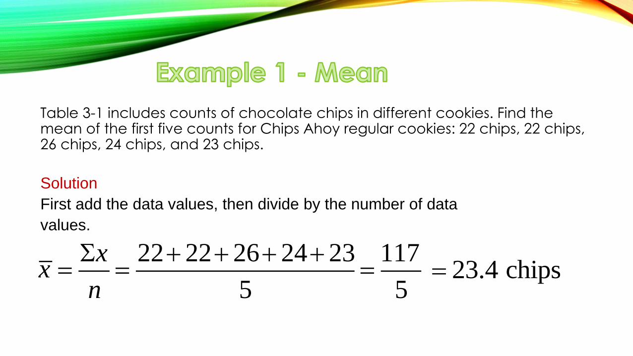
Table 3-1 includes counts of chocolate chips in different cookies. Find the mean of the first five counts for Chips Ahoy regular cookies: 22 chips, 22 chips, 26 chips, 24 chips, and 23 chips.

Solution

First add the data values, then divide by the number of data

values.

x

x

n

22 22 26 24 23

5

117

5 23.4 chips

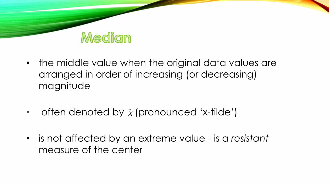
• the middle value when the original data values are

arranged in order of increasing (or decreasing)

magnitude

• often denoted by (pronounced ‘x-tilde’)

• is not affected by an extreme value - is a resistant

measure of the center

x

First sort the values (arrange them in order). Then –

1. If the number of data values is odd, the median is the number located in the exact middle of the list.

2. If the number of data values is even, the median is found by computing the mean of the two middle numbers.

5.40 1.10 0.42 0.73 0.48 1.10 0.66

Sort in order:

0.42 0.48 0.66 0.73 1.10 1.10 5.40

(in order - odd number of values)

Median is 0.73

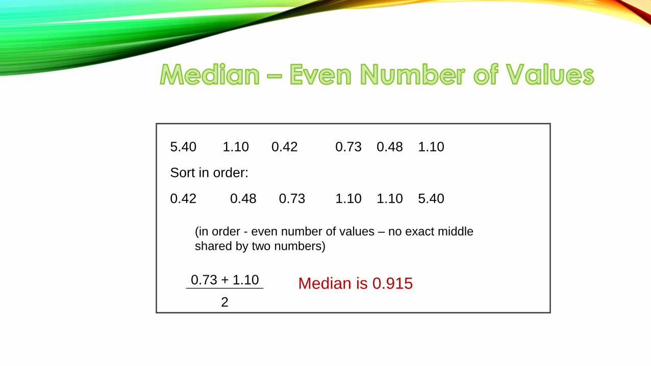
5.40 1.10 0.42 0.73 0.48 1.10

Sort in order:

0.42 0.48 0.73 1.10 1.10 5.40

0.73 + 1.10

2

(in order - even number of values – no exact middle

shared by two numbers)

Median is 0.915

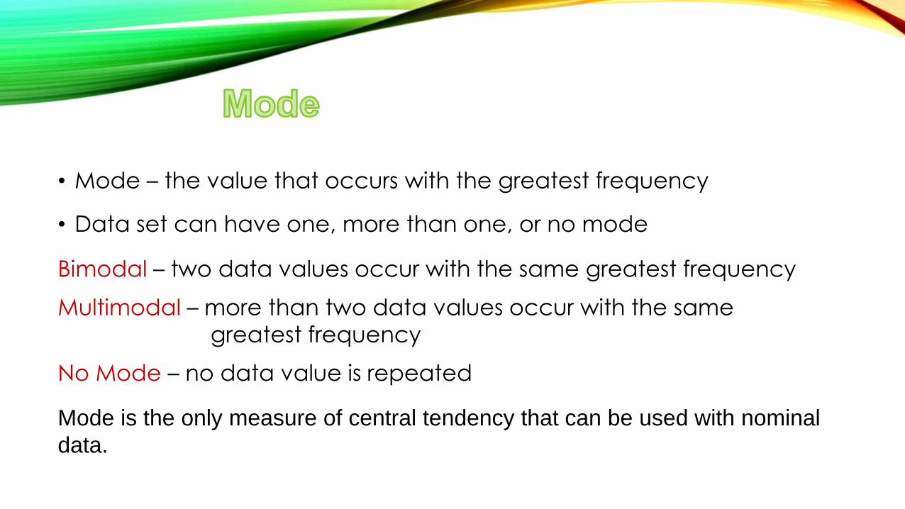
• Mode – the value that occurs with the greatest frequency

• Data set can have one, more than one, or no mode

Mode is the only measure of central tendency that can be used with nominal

data.

Bimodal – two data values occur with the same greatest frequency

Multimodal – more than two data values occur with the same

greatest frequency

No Mode – no data value is repeated

a. 5.40 1.10 0.42 0.73 0.48 1.10

b. 27 27 27 55 55 55 88 88 99

c. 1 2 3 6 7 8 9 10

Mode is 1.10

No Mode

Bimodal - 27 & 55

the value midway between the maximum and minimum values in the original data set

Midrange = maximum value + minimum value

2

Sensitive to extremes because it uses only the maximum and minimum

values, it is rarely used

Redeeming Features:

(1) very easy to compute

(2) reinforces that there are several ways to define the center

(3) avoid confusion with median by defining the midrange along

with the median

The range of a set of data values is the difference between the maximum data value and the minimum data value.

Range = (maximum value) – (minimum value)

It is very sensitive to extreme values; therefore, it is

not as useful as other measures of variation.

The standard deviation of a set of sample values, denoted by 𝑠, is a measure of how much data values deviate away from the mean.

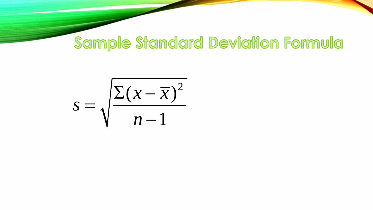
2( )

1

x xs

n

This formula is similar to the previous formula,

but the population mean and population size

are used.

2( )x

N

• The standard deviation is a measure of variation of all values from the

mean.

• The value of the standard deviation s is usually positive (it is never

negative).

• The value of the standard deviation s can increase dramatically with the

inclusion of one or more outliers (data values far away from all others).

• The units of the standard deviation s are the same as the units of the

original data values.

Population variance: σ2 - Square of the population

standard deviation σ

The variance of a set of values is a measure of variation

equal to the square of the standard deviation.

Sample variance: s2 - Square of the sample standard

deviation s

s = sample standard deviation

s2 = sample variance

= population standard deviation

= population variance 2

Find the standard deviation of these numbers of

chocolate chips: 22, 22, 26, 24

2

2 2 2 2

1

22 23.5 22 23.5 26 23.5 24 23.5

4 1

111.9149

3

x xs

n

It is based on the principle that for many data sets, the vast majority (such as 95%) of sample values lie within two standard deviations of the mean.

Minimum “usual” value (mean) – 2 (standard deviation) = 𝜇 − 2𝜎 =

Maximum “usual” value (mean) + 2 (standard deviation) = 𝜇 + 2𝜎 =

Informally define usual values in a data set to be those that are typical and not too extreme. Find rough estimates of the minimum and maximum “usual” sample values as follows:

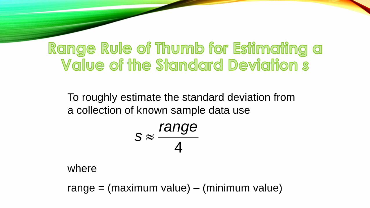
To roughly estimate the standard deviation from

a collection of known sample data use

where

range = (maximum value) – (minimum value)

4

ranges

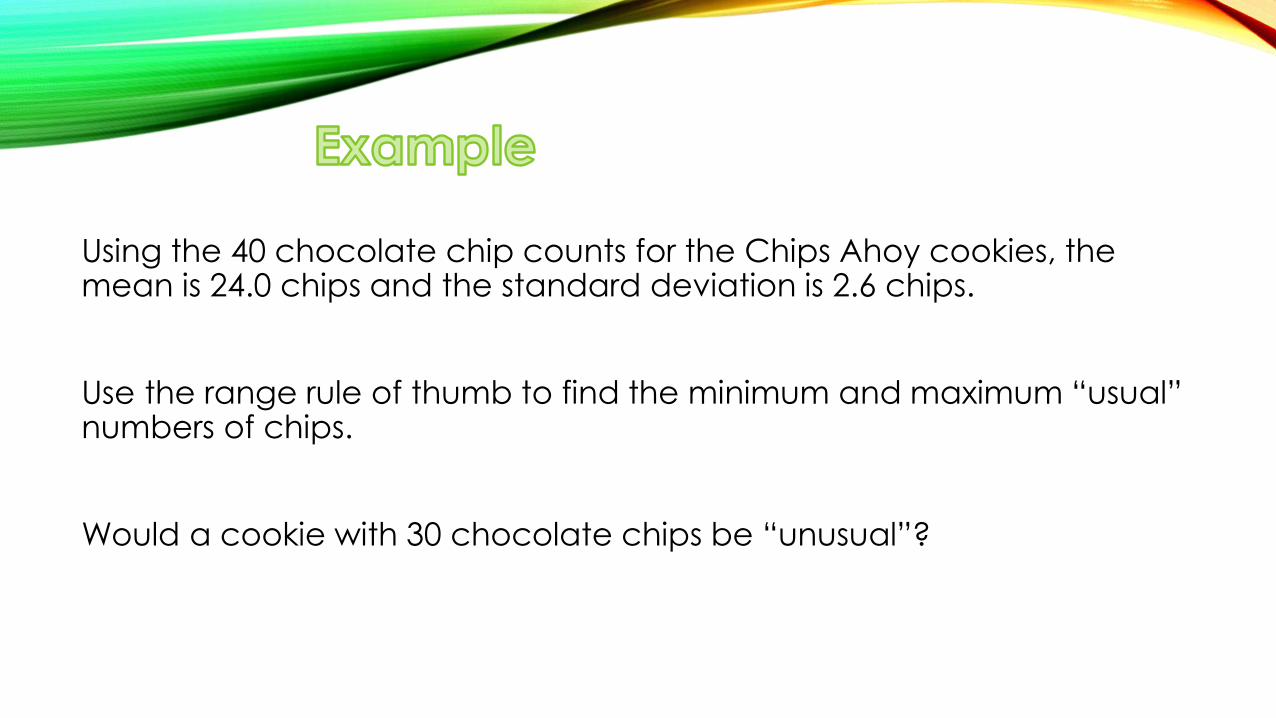
Using the 40 chocolate chip counts for the Chips Ahoy cookies, the mean is 24.0 chips and the standard deviation is 2.6 chips.

Use the range rule of thumb to find the minimum and maximum “usual” numbers of chips.

Would a cookie with 30 chocolate chips be “unusual”?

. . .

. . .

minimum "usual" value 24 0 2 2 6 18 8

maximum "usual" value 24 0 2 2 6 29 2

Because 30 falls above the maximum “usual” value, we can consider it

to be a cookie with an unusually high number of chips.

For data sets having a distribution that is approximately bell shaped, the

following properties apply:

About 68% of all values fall within 1 standard deviation of the mean.

About 95% of all values fall within 2 standard deviations of the mean.

About 99.7% of all values fall within 3 standard deviations of the mean.

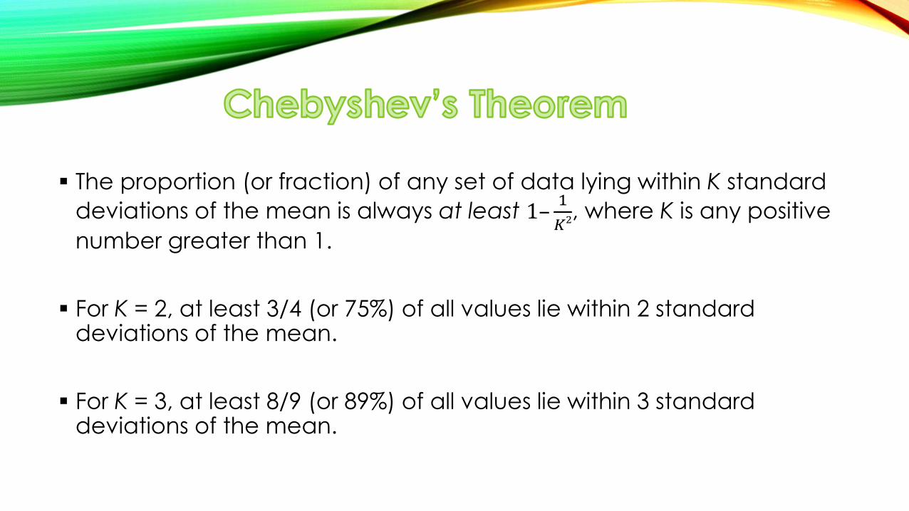
The proportion (or fraction) of any set of data lying within K standard

deviations of the mean is always at least 1–1

𝐾2, where K is any positive

number greater than 1.

For K = 2, at least 3/4 (or 75%) of all values lie within 2 standard deviations of the mean.

For K = 3, at least 8/9 (or 89%) of all values lie within 3 standard deviations of the mean.

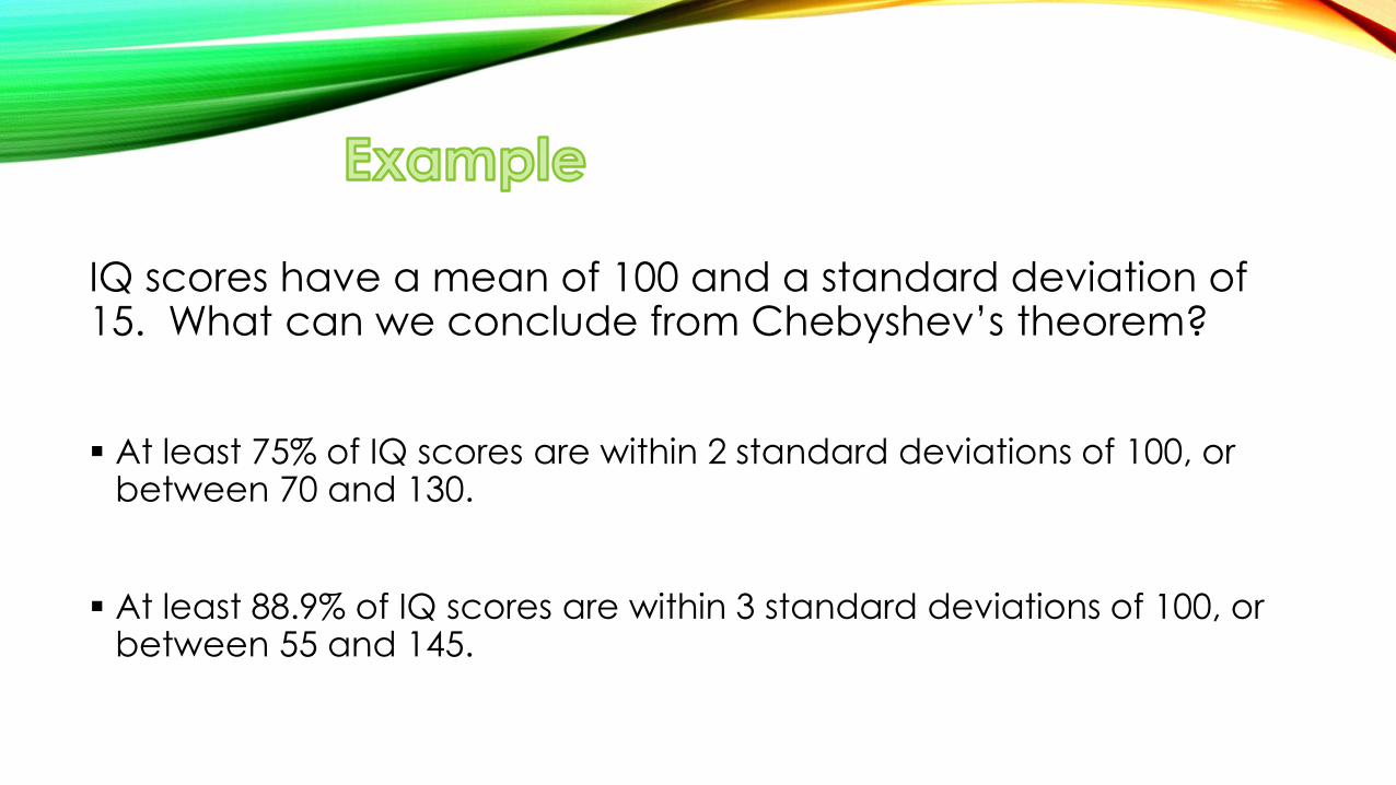
IQ scores have a mean of 100 and a standard deviation of 15. What can we conclude from Chebyshev’s theorem?

At least 75% of IQ scores are within 2 standard deviations of 100, or between 70 and 130.

At least 88.9% of IQ scores are within 3 standard deviations of 100, or between 55 and 145.

It’s a good practice to compare two sample standard deviations only when the sample means are approximately the same.

When comparing variation in samples with very different means, it is better to use the coefficient of variation.

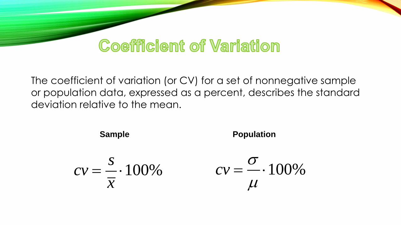
The coefficient of variation (or CV) for a set of nonnegative sample

or population data, expressed as a percent, describes the standard

deviation relative to the mean.

Sample Population

100%s

cvx

100%cv

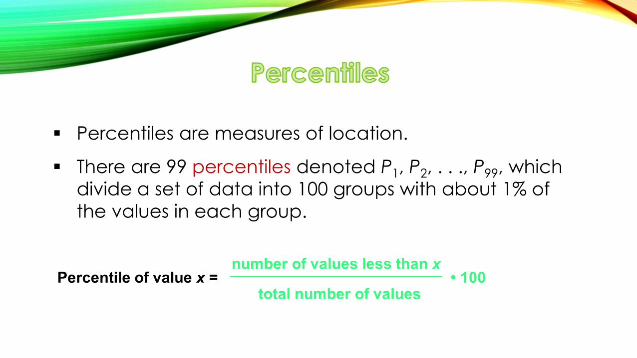
Percentiles are measures of location.

There are 99 percentiles denoted P1, P2, . . ., P99, which

divide a set of data into 100 groups with about 1% of

the values in each group.

For the 40 Chips Ahoy cookies, find the percentile for a cookie with

23 chips.

Answer: We see there are 10 cookies with fewer than 23 chips, so

A cookie with 23 chips is in the 25th percentile.

10Percentile of 23 100 25

40

n total number of values in the

data set

k percentile being used

L locator that gives the position of

a value

Pk kth percentile

Notation

100

kL n

Are measures of location, denoted Q1, Q2, and Q3,

which divide a set of data into four groups with about

25% of the values in each group.

Q1 (First quartile) separates the bottom 25% of sorted

values from the top 75%.

Q2 (Second quartile) same as the median; separates the

bottom 50% of sorted values from the top 50%.

Q3 (Third quartile) separates the bottom 75% of sorted

values from the top 25%.

Q1, Q2, Q3 divide sorted data values into four equal parts

25% 25% 25% 25%

Q3 Q2 Q1 (minimum) (maximum)

(median)

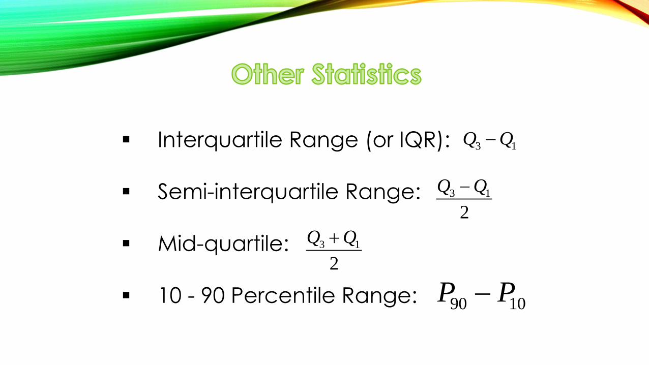
Interquartile Range (or IQR):

Semi-interquartile Range:

Mid-quartile:

10 - 90 Percentile Range:

3 1

2

Q Q

3 1Q Q

3 1

2

Q Q

90 10P P

For a set of data, the 5-number summary consists of these five

values:

1. Minimum value

2. First quartile Q1

3. Second quartile Q2 (same as median)

4. Third quartile, Q3

5. Maximum value

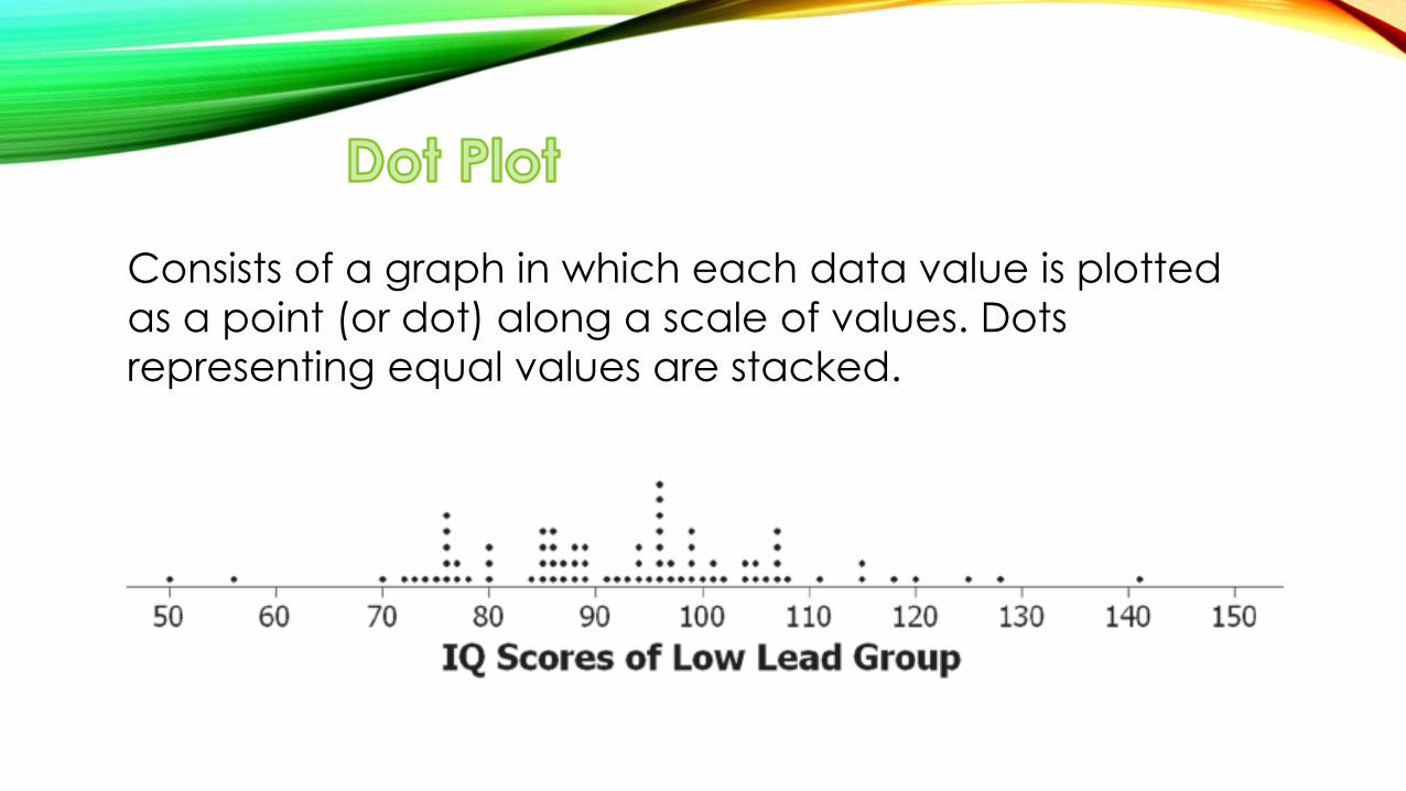
Consists of a graph in which each data value is plotted

as a point (or dot) along a scale of values. Dots

representing equal values are stacked.

represents quantitative data by separating each value into

two parts: the stem (such as the leftmost digit) and the leaf

(such as the rightmost digit).

A graph consisting of bars of equal width drawn

adjacent to each other (unless there are gaps in the

data)

The horizontal scale represents the classes of

quantitative data values and the vertical scale

represents the frequencies.

The heights of the bars correspond to the frequency

values.

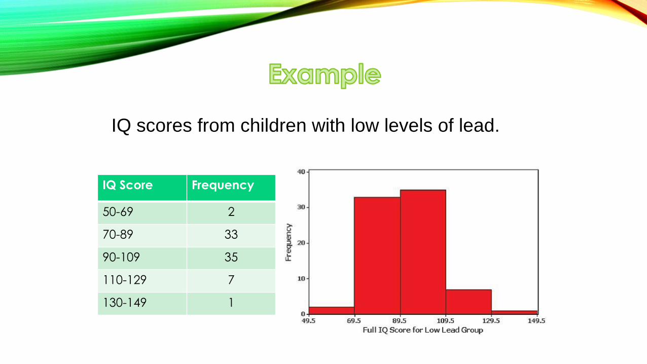
IQ scores from children with low levels of lead.

IQ Score Frequency

50-69 2

70-89 33

90-109 35

110-129 7

130-149 1

has the same shape and horizontal scale as a histogram, but the

vertical scale is marked with relative frequencies instead of actual

frequencies

IQ Score Relative Frequency

50-69 2.6%

70-89 42.3%

90-109 44.9%

110-129 9.0%

130-149 1.3%

A boxplot (or box-and-whisker-diagram) is a graph of a data set that

consists of a line extending from the minimum value to the maximum

value, and a box with lines drawn at the first quartile, Q1, the median,

and the third quartile, Q3.

Normal Distribution:

Heights from a Simple Random Sample of Women

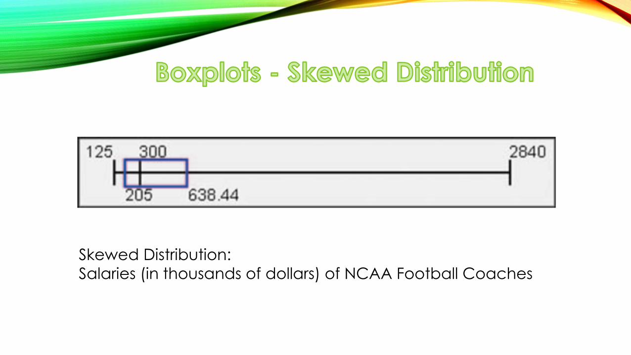
Skewed Distribution:

Salaries (in thousands of dollars) of NCAA Football Coaches

An outlier is a value that lies very far away from the vast majority of the other values in a data set.

An outlier can have a dramatic effect on the mean and the standard deviation.

An outlier can have a dramatic effect on the scale of the histogram so that the true nature of the distribution is totally obscured.

For purposes of constructing modified boxplots, we can consider

outliers to be data values meeting specific criteria.

In modified boxplots, a data value is an outlier if it is:

above Q3 by an amount greater than 1.5 IQR

below Q1 by an amount greater than 1.5 IQR

or

Boxplots described earlier are called skeletal (or regular) boxplots.

Some statistical packages provide modified boxplots which represent outliers as special points.

A special symbol (such as an asterisk) is used to identify

outliers.

The solid horizontal line extends only as far as the minimum

data value that is not an outlier and the maximum data

value that is not an outlier.

A modified boxplot is constructed with these specifications:

the number of standard deviations that a given value x is above or below the mean

Whenever a value is less than the mean, its

corresponding z score is negative

Ordinary values:

Unusual Values:

2 score 2z

score 2 or score 2z z

48 67.31.87

10.3

x xz

s

The author of the text measured his pulse rate to be 48 beats per minute.

Is that pulse rate unusual if the mean adult male pulse rate is 67.3 beats per minute with a standard deviation of 10.3?

Answer: Since the z score is between – 2 and +2, his pulse rate is not unusual.

The sampling distribution of the sample mean is the distribution of all possible sample means, with all samples having the same sample size n taken from the same population.

Sample means target the value of the population mean. (That is, the mean of the sample means is the population mean.)

The distribution of the sample means tends to be a normal distribution.

Consider repeating this process: Roll a die 5 times. Find

the mean .

What do we know about the behavior of all sample means

that are generated as this process continues indefinitely?

x

All outcomes are equally likely, so the population mean is 3.5; the

mean of the 10,000 trials is 3.49. If continued indefinitely, the sample

mean will be 3.5. Also, notice the distribution is “normal.”

Specific results from 10,000 trials

Sample means, variances and proportions are unbiased estimators.

That is they target the population parameter.

These statistics are better in estimating the population parameter.

Sample medians, ranges and standard deviations are biased estimators.

That is they do NOT target the population parameter.

Note: the bias with the standard deviation is relatively small in large samples so s is often used to estimate.

Given:

1) The random variable x has a distribution (which may or may not be normal) with mean μ and standard deviation σ.

2) Simple random samples all of size n are selected from the population. (The samples are selected so that all possible samples of the same size n have the same chance of being selected.)

Conclusions:

The distribution of sample will, as the sample size increases, approach a normal distribution.

The mean of the sample means is the population mean .

The standard deviation of all sample means is .

x

/ n

1) For samples of size n larger than 30, the distribution of the sample means can be approximated reasonably well by a normal distribution. The approximation becomes closer to a normal distribution as the sample size n becomes larger.

2) If the original population is normally distributed, then for any sample

size n, the sample means will be normally distributed (not just the

values of n larger than 30).

The mean of the sample means

The standard deviation of sample mean

(often called the standard error of the mean)

x

xn

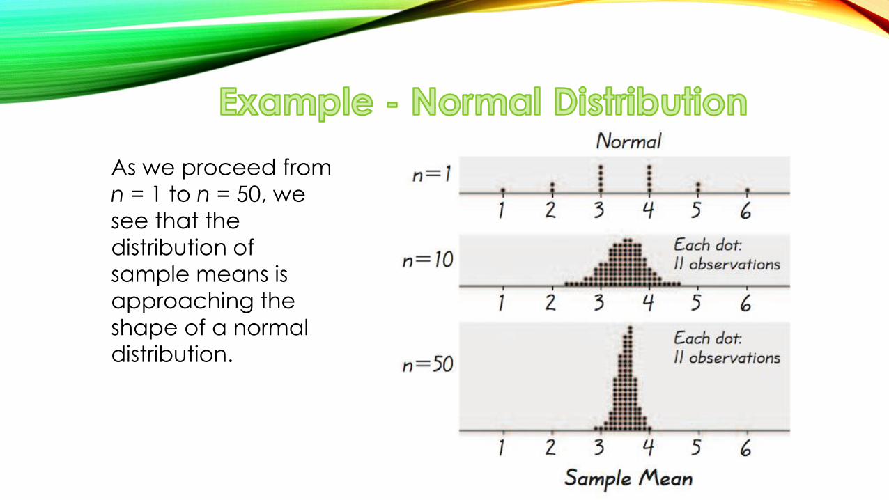
As we proceed from

n = 1 to n = 50, we

see that the

distribution of

sample means is

approaching the

shape of a normal

distribution.

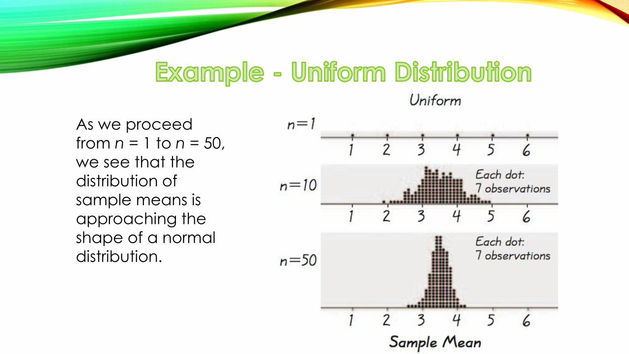
As we proceed

from n = 1 to n = 50,

we see that the

distribution of

sample means is

approaching the

shape of a normal

distribution.

As we proceed from

n = 1 to n = 50, we

see that the

distribution of sample

means is

approaching the

shape of a normal

distribution.

As the sample size increases, the sampling distribution of sample means approaches a normal distribution.

Suppose an elevator has a maximum capacity of 16 passengers with a total weight of 2500 lb. Assuming a worst case scenario in which the passengers are all male, what are the chances the elevator is overloaded? Assume male weights follow a normal distribution with a mean of 182.9 lb. and a standard deviation of 40.8 lb.

a) Find the probability that 1 randomly selected male has a weight greater than 156.25 lb.

b) Find the probability that a sample of 16 males have a mean weight greater than 156.25 lb. (which puts the total weight at 2500 lb., exceeding the maximum capacity).

a) Find the probability that 1 randomly selected male has a weight greater than 156.25 lb. Using StatCrunch, the area to the right is 0.7432.

b) Find the probability that a sample of 16 males have a mean weight greater than 56.25 lb. Since the distribution of male weights is assumed to be normal, the sample mean will also be normal.

Using StatCrunch, the area to the right is 0.9955.

182.9

40.810.2

16

x x

xx

n

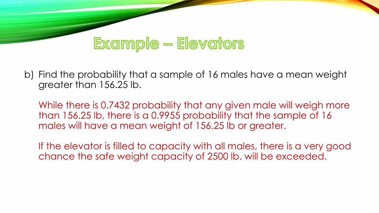
b) Find the probability that a sample of 16 males have a mean weight greater than 156.25 lb. While there is 0.7432 probability that any given male will weigh more than 156.25 lb, there is a 0.9955 probability that the sample of 16 males will have a mean weight of 156.25 lb or greater. If the elevator is filled to capacity with all males, there is a very good chance the safe weight capacity of 2500 lb. will be exceeded.