design fundamentals of electrical machines and drive systems

Chapter 2Design Fundamentals of ElectricalMachines and Drive Systems

Abstract This chapter presents a brief summary of the design fundamentalsincluding the analysis models and methods for electrical machines and drive sys-tems, based on our design experiences, particularly for permanent magnet electricalmachine with soft magnetic composite cores. Because of the multi-disciplinarynature, these design models and methods will be investigated at the disciplinarylevel, including electromagnetic, thermal, mechanical, power electronics, andcontrol algorithm designs. Several design examples will be presented to illustratethe corresponding design models and methods based on our research findings, suchas the finite element model for design analysis of motors, and the model predictivecontrol algorithm and its improvement form for the drive systems. These modelsand algorithms will be employed in the design optimization of electrical machinesand drive systems in the following chapters.

Keywords Electrical drive systems � Electromagnetic design � Thermal design �Mechanical design � Power electronics design � Control algorithms � Finite elementmodel � Model predictive control

2.1 Introduction

2.1.1 Framework of Multi-disciplinary Design

Figure 2.1 illustrates a general framework of multi-disciplinary design for electricalmachines and drive systems. As shown, three main components, i.e., motor, powerelectronics and controller, have to be investigated when designing such electricaldrive systems [1, 2]. The main design procedure includes the following steps.

Firstly, define the specifications of the electrical machine and drive systemrequired by a given application, which include the steady state specifications, suchas the rated power, speed range, voltage, current, efficiency, power factor (in case ofAC machines), volume and cost, and dynamic performances, such as the maximumovershoot, settling time, and stability.

© Springer-Verlag Berlin Heidelberg 2016G. Lei et al., Multidisciplinary Design Optimization Methodsfor Electrical Machines and Drive Systems, Power Systems,DOI 10.1007/978-3-662-49271-0_2

25

Secondly, select a type of the motor, power electronic converter, and controlalgorithm from possible options. The motor options include permanent magnet(PM) motors, induction machines, synchronous machines, DC machines, and swit-ched reluctance machines. For servo drives, stepping motors and other types of servomotors can be considered. In this step, different motor topologies have to be inves-tigated as well. The power electronic converter options mainly include the differenttopologies of AC/DC, DC/DC, and DC/AC converters. The controller design mainlyinvestigates the control strategies and algorithms, such as field oriented control(FOC), direct torque control (DTC), and model predictive control (MPC).

Thirdly, based on the selected motor type, converter circuit, and control scheme,various disciplinary-level analyses should be conducted to evaluate the performanceof the drive system. For example, the motor design analysis consists of mainly theelectromagnetic, thermal and mechanical analyses (the shaded boxes in the figure).Coupled-field analyses may be required in the design process, such aselectromagnetic-thermal and electromagnetic-mechanical stress analyses.

In summary, the design of electrical machines and drive systems mainly consistsof the analyses of five coupled disciplines or domains: electromagnetic, thermal,mechanical, power electronics, and controller designs. The following sections willpresent the popular design analysis models and methods for each discipline.

2.1.2 Power Losses and Efficiency

Power losses and efficiency are two main issues in the design analysis of electricalmachines and drive systems. The power losses are mainly composed of the copperloss, core loss, mechanical loss, and stray loss.

Fig. 2.1 Multi-disciplinary design framework of electrical machines and drive systems

26 2 Design Fundamentals of Electrical Machines and Drive Systems

(1) The copper loss or Ohmic loss: PCu ¼ I2R is the power dissipated in stator androtor windings due to the resistance of copper wire, where I is the windingcurrent and R the winding resistance. Normally the DC resistance is used inthe calculation. However, it should be noted that the winding resistancedepends on the operating conditions, i.e., temperature and frequency (due tothe skin effects). In case of the brushes and slip rings/commutator, the effect ofcontact resistance is often accounted for by assuming a voltage drop of 2 V.

(2) The core loss is the power dissipated in a magnetic core due to the variation ofmagnetic field. This occurs in the stator and/or rotor iron core of an electricalmachine subject to AC excitations. Practically, it can be measured byopen-circuit or no-load tests. When the magnetic material is under an alter-nating sinusoidal flux excitation, the alternating core loss can be calculated by

Pa ¼ ChafBh þCeaðfBÞ2 þCaaðfBÞ1:5 ð2:1Þ

where f is the excitation frequency, B the magnitude of sinusoidal magneticflux density, and Cha, Cea, Caa, and h are the alternating core loss coefficients.In case of rotating electrical machines, the rotational core losses have to beconsidered. Figure 2.2 plots the average core losses with alternating fluxdensity from 2 to 2,000 Hz and circular rotating flux density vectors from 5 to1,000 Hz of a cubic soft magnetic composite (SMC) SOMALYTM 500 sample[3]. These are the standard core loss data used to identify the core loss modelparameters. The circularly rotational core loss can be calculated by

Pr ¼ Phr þCerðfBÞ2 þCarðfBÞ1:5 ð2:2Þ

where

Phr

f¼ a1

1=s

ða2 þ 1=sÞ2 þ a23� 1=ð2� sÞ½a2 þ 1=ð2� sÞ�2 þ a23

" #

and

s ¼ 1� BBs

ffiffiffiffiffiffiffiffiffiffiffiffiffiffiffiffiffiffiffiffiffiffiffiffiffiffiffiffiffiffiffiffiffiffi1� ½1=ða22 þ a23Þ�

q

Bs is the saturation flux density, and Cer, Car, a1, a2 and a3 are the rotationalcore loss coefficients.When the material is under a two dimensional elliptically rotating B excitation,the core loss can be computed by

Per ¼ RBPr þð1� RBÞ2Pa ð2:3Þ

2.1 Introduction 27

where RB ¼ Bmin=Bmaj is the axis ratio, Bmin and Bmaj are the magnitudes ofthe minor and major axes of the ellipse, respectively, and Pr and Pa thecorresponding rotational and alternating core losses when B = Bmaj. Moredetails about the rotational core losses can be found in [3–9].

(3) The mechanical losses are the power losses caused by the friction (brushes,slip rings/commutator, shaft and bearing), damping, windage, and cooling fan.It can be approximately determined by no-load test. In design, empirical dataare used.

(4) The stray loss is the power loss caused by stray factors that are hard todetermine separately, such as the non-uniform current distribution in con-ductors and additional core loss due to distorted magnetic flux distribution forvarious reasons. Because it is usually difficult to determine accurately the strayloss, estimations based on experimental tests and empirical judgment are

Fig. 2.2 Average core lossesunder a alternating andb circular rotating magneticfluxes [3]


acceptable. For most types of machines, this can be assumed to be 1 % of theoutput power.

In most electrical machines, the stator and/or rotor cores subject to varyingmagnetic fluxes are made of laminated silicon steels, which have low core loss, andhence the major power loss is the copper loss. Depending on the type of machine,the copper loss normally accounts for 80–90 % of the total loss.

Based on the above analysis, the efficiency of a machine can be calculated by

g ¼ Pout

Pin¼ Pin � ðPCu þPCore þPMec þPStrayÞ

Pinð2:4Þ

Typical values of full load efficiency for rotating machines are:

• 50 % or less for fractional horse power motors (a few W to a few hundreds ofW),

• 75–85 % for electrical machines of 1 kW to a few tens of kW,• 85–95 % for electrical machines of 100 kW to 1 MW, and• 95–98 % or above for electrical machines of 1 MW to a few hundreds of MW

(e.g. 98 % for 100 MVA turbo generator).

2.2 Electromagnetic Design

Since electrical machines are electromagnetic devices for transforming electricalpower at one voltage to another (transformers) or converting electric power intomechanical power or vice versa (motors or generators) by the principle of elec-tromagnetic induction, electromagnetic design is a fundamental design stage ofelectrical machines and drive systems, and is usually based on the following threekinds of analysis models: the analytical model, magnetic circuit model, and finiteelement model (FEM) [10–20].

2.2.1 Analytical Model

Analytical model is generally used to calculate the performance indicators ofelectrical machines, such as the output power, torque, and cogging torque. Forexample, the power and sizing equations are the powerful ways to guide the designof PM motors [10, 11]. By utilizing the current density in the sizing equation, somebasic internal relationships can be found among the main dimensions to maximizethe torque density.

Assuming the flux linkage of stator winding in a PM motor is sinusoidal, andignoring the winding resistance, the input power Pin can be expressed by

2.1 Introduction 29

Pin ¼ mT

ZT0

eðtÞiðtÞdt ¼ mT

ZT0

Emsin2pT

t

� �Imsin

2pT

t

� �dt ¼ m

2EmIm ð2:5Þ

where m is the number of phases, Em the peak value of back electromotive force(EMF), Im the peak value of phase current, and T the electrical time period. Theoutput torque can be calculated by

Tout ¼ Pout

xr¼ g

m2pkpKsf AsJm ð2:6Þ

where η is the efficiency, p the number of pole pairs, λp the peak value of PM fluxlinkage, ωr the mechanical rotary speed, Ksf the slot fill factor, As the slot area, andJm the peak of current density. For different kinds of PM motors, λp and As arerelated differently to their dimensions [21–23].

2.2.2 Magnetic Circuit Model

The magnetic circuit model acts as a uniform principle in descriptive magneto-statics, and as an approximate computational aid in electrical machine design. Themodel uses the conception of magnetic reluctance to establish an equivalent circuitfor approximate analysis of static magnetic field in electrical machines [24]. Toillustrate this model, a PM transverse flux machine (TFM) designed by SMCmaterial is investigated.

The SMC material is a relatively new soft magnetic material that has manyadvantages over the conventional silicon steel sheets. The main advantages of SMCmaterial are the magnetic and mechanical isotropy and low cost, high productivity,and high quality manufacturing capability of complex electromagnetic componentsby the matured powder metallurgical molding technology, which will enable lowcost high productivity commercial manufacturing of SMC motors for a great varietyof electrical appliances [24–32].

In our previous work, a 3D flux PM TFM with SMC stator core was developed.Figure 2.3 shows a photo of the PM-SMC TFM prototype. This machine wasinitially designed to deliver an output power of 640 W at 1800 rev/min. It has 20poles in the external PM rotor, i.e., 120 PMs in the rotor and 60 SMC teeth in thestator. The stator core is made of SMC SOMALOYTM 500. The operating fre-quency of this motor is 300 Hz at 1800 rev/min. Table 2.1 tabulates the main designdimensions for this TFM [24, 25].

In order to briefly predict the performance of this TFM, a sketchy magnetic circuitmodel as shown in Fig. 2.4 can be used. Figure 2.4 illustrates the main flux circuitmodel and flux path of this TFM, where the resistances represent the magneticreluctances and the current source (PhiPM) stands for the magneto-motive forces(mmfs) of PMs, and thus Rry represents the magnetic reluctance of rotor, Rm the


magnetic reluctance of PM, Rg the magnetic reluctance of the air gap, Rst1 themagnetic reluctance of the stator teeth, Rst2 and Rsy stand for the magnetic reluctanceof the stator yoke. By analyzing this model, the main magnetic flux can be calculated.

Meanwhile, the magnetic flux leakage is a serious problem in this TFM, thus itshould be considered in the magnetic circuit model. Several flux leakage modelscan be constructed for this TFM. Figure 2.5 illustrates the main flux leakage model.In this model, the adjacent PM in the one side of the machine is modeled, whereRry1 represents the magnetic reluctance of rotor, Rg1 and Rg2 represent the magneticreluctance of the air gap, Rs1 stands for the magnetic reluctance of the stator.

With the computed flux linkage, the resultant magnetic flux density in the air gapand the flux per turn of coil can be estimated. After calculation, the obtained fluxper turn of this PM-SMC TFM is 0.32 mWb, which is higher than the calculatedresult (0.28 mWb) by using the FEM [24].

This model can be also used to evaluate the performance of the motor. Based onthe calculated magnetic flux of the motor, the flux linkage per phase equals the

(a) (b)

Fig. 2.3 Photo of the PM-SMC TFM prototype, a PM rotor, and b 3 stack SMC stator

Table 2.1 Main designdimensions of PM-SMC TFM

Par. Description Unit Value

– Number of phases – 3

– Number of poles – 20

– Number of stator teeth – 60

– Number of magnets – 120

– Stator outer radius mm 40

– Effective stator axial length mm 93

x1 PM circumferential angle degree 12

x2 PM width mm 9

x3 SMC tooth circumferential width mm 9

x4 SMC tooth axial width mm 8

x5 SMC tooth radial height mm 10.5

x6 Number of turns – 125

x7 Diameter of copper wire mm 1.25

x8 Air gap length mm 1.0

2.2 Electromagnetic Design 31

number of coil turns multiplied by the magnetic flux of each coil turn, and it can becomputed as

kPM ¼ klNcoilpUgap ð2:7Þ

where λPM is the PM flux linkage per phase, kl the leakage coefficient, Ncoil thenumber of turns of the phase winding, p the number of pole pairs, and Φgap is fluxper coil turn. The back EMF can be expressed as

(b)

(a)

Fig. 2.4 Main flux circuit and flux path of the PM-SMC TFM, a magnetic circuit model, b fluxpath in 2D plane

(a)

(b)

Fig. 2.5 Flux leakage circuit and path of the PM-SMC TFM, a magnetic circuit model, b leakagepath in 2D plane


Em ¼ xekPM ¼ pxmkPM ð2:8Þ

where ωe = pωm is the electrical angular frequency, and ωm the mechanical angularspeed. The electromagnetic torque Tem can be expressed as

Tem ¼ Pem

xm¼

ffiffiffi2

p

2mpkPMIm ð2:9Þ

After the calculation, the no-load back EMF is 53.26 V at the rated speed of1800 rev/min. According to (2.9), the electromagnetic torque is 4.66 Nm at therated current of 5.5 A (RMS value). Compared to the electromagnetic torqueobtained from FEM, i.e., 4.08 Nm, the relative error is about 0.58/4.08 = 14.21 %.

2.2.3 Finite Element Model

FEM is a widely used analysis model for field analysis in electrical machines aswell as other electromagnetic devices. The theory of FEM can be found in manybooks and research papers. The PM-SMC TFM investigated above will beemployed as an example to show the application of FEM for designing electricalmachines.

When analyzing the magnetic field distribution, we used field analysis softwarepackage ANSYS, and taking advantage of the periodical symmetry, we only needto analyze one pole-pair region of the machine, as shown in Fig. 2.6a. At the tworadial boundary planes, the magnetic scalar potential obeys the periodical boundaryconditions:

umðr;Dh; zÞ ¼ umðr;�Dh; zÞ ð2:10Þ

Fig. 2.6 a One pole pitch of FEM solution region for one phase (stack), and b magnetic fielddistribution under no-load


where Dh ¼ 18� mechanical is the angle of one pole pitch. The origin of thecylindrical coordinate is located at the center of the stack.

Figure 2.6b illustrates the magnetic field distribution under no-load. Based onthe FEM analysis, the calculated key motor parameters for this machine are listed inTable 2.2. The measured parameters are also listed in the table to show the effec-tiveness of the FEM method. As shown, the measured motor back EMF constant is0.244 Vs, 1 % lower than the calculated value of 0.247 Vs. The calculated phaseresistance and inductance, and maximal cogging torque are 0.310 Ω, 6.68 mH and0.339 Nm, respectively, which are very close to the measured values (0.305 Ω,6.53 mH and 0.320 Nm). In summary, the estimated parameters calculated by theFEM-based method are well aligned with the experimental results. Therefore, FEMis better than magnetic circuit model, and it is reliable to be used for optimization ofthe electromagnetic design of electrical machines.

Moreover, the output performance parameters, such as output power, torque andefficiency, can be estimated with the calculated electromagnetic parameters men-tioned above. In the estimation, the control method is assumed to maintain that thed-axis component of current equals zero. Figure 2.7 shows the per phase equivalentelectric circuit of this motor under the assumed control method.

Based on this per phase equivalent electrical circuit, the main relationships of themotor can be predicted by

Vin ¼ffiffiffiffiffiffiffiffiffiffiffiffiffiffiffiffiffiffiffiffiffiffiffiffiffiffiffiffiffiffiffiffiffiffiffiffiffiffiffiffiffiffiffiffiffiffiffiffiffiðEa þ IaRaÞ2 þðxeLaIaÞ2

qð2:11Þ

Pin ¼ 3VinIa cosu ð2:12Þ

Pout ¼ Pin � Pcore � Pcopper � Pmech ð2:13Þ

Tout ¼ Pout

xrð2:14Þ

where Vin is the input voltage, Ea the back EMF, Ia the armature current, ωe theelectric angular frequency, La the inductance, Ra the resistance, φ the angle betweenVin and Ea, Pin the input power, Pout the output power, Pcore the core loss, Pcopper

the copper loss, Pmech the mechanical loss, Tout the output torque, and ωr themechanical angular speed.

In motor with SMC cores, unlike the conventional motors made of silicon sheetsteels, the core loss can be a major part among all power losses, and the mechanical

Table 2.2 Key PM-SMCTFM parameters

Parameter Unit Calculated Measured

Motor back EMFconstant

Vs 0.247 0.244

Phase resistance Ω 0.310 0.305

Phase inductance mH 6.68 6.53

Maximal cogging torque Nm 0.339 0.320


loss is generally considered as 1–1.5 % of the output power. In general, the coreloss prediction in the TFM should be calculated by using the FEM based on themulti-frequency core loss characteristic of the material. More comparison resultscan be seen in [24, 25].

2.3 Thermal Design

2.3.1 Thermal Limits in Electrical Machines

The rating of an electrical machine gives its working capability under the specifiedelectrical and environmental conditions. Major factors that determine the ratings arethermal and mechanical considerations. To obtain an economic utilization of thematerials and safe operation of the motor, it is necessary to predict with reasonableaccuracy the temperature rise of the internal parts, especially in the coils andmagnets.

The temperature rise resulted from the power losses in an electrical machineplays a key role in rating the power capacity of the machine, i.e., the amount ofpower it can convert without being burnt for a specified length of life time. The lifeexpectancy of a large industrial electrical machine ranges from 10 to 50 years ormore. In an aircraft or electronic equipment, it can be of the order of a few thousandhours, whereas in a military application, e.g. missile, it can be only a few minutes.

Fig. 2.7 Per phase equivalentelectric circuit and phasordiagrams of the motor


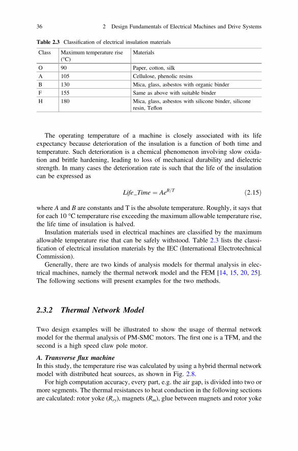
The operating temperature of a machine is closely associated with its lifeexpectancy because deterioration of the insulation is a function of both time andtemperature. Such deterioration is a chemical phenomenon involving slow oxida-tion and brittle hardening, leading to loss of mechanical durability and dielectricstrength. In many cases the deterioration rate is such that the life of the insulationcan be expressed as

Life Time ¼ AeB=T ð2:15Þ

where A and B are constants and T is the absolute temperature. Roughly, it says thatfor each 10 °C temperature rise exceeding the maximum allowable temperature rise,the life time of insulation is halved.

Insulation materials used in electrical machines are classified by the maximumallowable temperature rise that can be safely withstood. Table 2.3 lists the classi-fication of electrical insulation materials by the IEC (International ElectrotechnicalCommission).

Generally, there are two kinds of analysis models for thermal analysis in elec-trical machines, namely the thermal network model and the FEM [14, 15, 20, 25].The following sections will present examples for the two methods.

2.3.2 Thermal Network Model

Two design examples will be illustrated to show the usage of thermal networkmodel for the thermal analysis of PM-SMC motors. The first one is a TFM, and thesecond is a high speed claw pole motor.

A. Transverse flux machineIn this study, the temperature rise was calculated by using a hybrid thermal networkmodel with distributed heat sources, as shown in Fig. 2.8.

For high computation accuracy, every part, e.g. the air gap, is divided into two ormore segments. The thermal resistances to heat conduction in the following sectionsare calculated: rotor yoke (Rry), magnets (Rm), glue between magnets and rotor yoke

Table 2.3 Classification of electrical insulation materials

Class Maximum temperature rise(°C)

Materials

O 90 Paper, cotton, silk

A 105 Cellulose, phenolic resins

B 130 Mica, glass, asbestos with organic binder

F 155 Same as above with suitable binder

H 180 Mica, glass, asbestos with silicone binder, siliconeresin, Teflon


(Rmg), air gap (Rag), stator yoke (RFe1), stator side discs (RFe2), stator teeth (RFe3),varnished copper wire (Rcu), and insulations (RI1, RI2, RI3) between the winding andthe stator yoke, the stator wall disc, and the air gap, respectively. In addition, thethermal resistances of the stator shaft (Rss), the aluminum end plates (Ral), and thestationary air (Rsa) between the side stator discs and the end plates are calculatedseparately [25].

The equivalent thermal resistances to the heat convection of the followingsections are calculated: that between the stator tooth surface and the inner air in theair gap (RFeA), that between the winding and the inner air (RWA), that between themagnet and the inner air (RmA), that between the rotor yoke and the inner air(RryA1), and that between the rotor yoke and the outer air (RryA2).

The heat sources include the stator winding copper losses (Pcu), the stator androtor core losses (PFes, PFer), and the mechanical losses due to windage and friction(Pmec). The improved method for core loss calculation can obtain the loss distri-bution, which is a great advantage for thermal calculation by the hybrid thermalmodel.

The temperature rises in the middle of several parts are calculated as 64.9 °C inthe stator winding, 78.6 °C in the stator core, 59.3 °C in the air gap, 36.1 °C in themagnets, and 25.3 °C in the rotor yoke outer surface. The experimentally measuredresults are 66 °C in the stator winding and 27 °C in the rotor yoke, and it can beseen that the maximum relative error between the calculated and measured results isonly 3 %. Thus, it is reliable to use the thermal network method for design of thisTFM.

Fig. 2.8 Thermal network model of the TFM prototype

2.3 Thermal Design 37

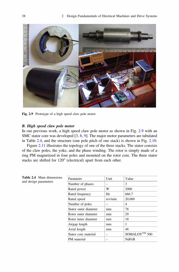
B. High speed claw pole motorIn our previous work, a high speed claw pole motor as shown in Fig. 2.9 with anSMC stator core was developed [3, 8, 9]. The major motor parameters are tabulatedin Table 2.4, and the structure (one pole pitch of one stack) is shown in Fig. 2.10.

Figure 2.11 illustrates the topology of one of the three stacks. The stator consistsof the claw poles, the yoke, and the phase winding. The rotor is simply made of aring PM magnetized in four poles and mounted on the rotor core. The three statorstacks are shifted for 120o (electrical) apart from each other.

Fig. 2.9 Prototype of a high speed claw pole motor

Table 2.4 Main dimensionsand design parameters

Parameter Unit Value

Number of phases – 3

Rated power W 2000

Rated frequency Hz 666.7

Rated speed rev/min 20,000

Number of poles – 4

Stator outer diameter mm 78

Rotor outer diameter mm 29

Rotor inner diameter mm 18

Airgap length mm 1

Axial length mm 48

Stator core material – SOMALOYTM 500

PM material – NdFeB


In general, the geometrical complexity of an electrical machine requires a largethermal network if a high resolution of temperature distribution is required. Insteadof using a whole model, the geometrical symmetries of the machine can be used toreduce the size of the model. The distributed thermal properties have been lumpedtogether to form a small thermal network, representing the whole machine. For thecalculation of temperature distribution in the SMC motor, a thermal resistancenetwork, as shown in Fig. 2.12, is used. It has ten nodes (the outer air, frame, yoke,and so on). Each node represents a specific part or region of the machine, and thethermal resistances (Rn, n = 1,…,16) between the nodes include complex processes,

Fig. 2.10 Magneticallyrelevant parts of one stack ofthree-phase claw pole motor

Fig. 2.11 Structure of ahigh-speed claw pole motor(one pole pitch of one stack)


such as the 2D and 3D heat flow, convection, internal heat generation, and varia-tions in material properties. To account for the three dimensional heat flows at anode, the thermal structure shown in Fig. 2.13 can be employed.

As shown in Fig. 2.13, the thermal resistances of an element are built in threedirections, and the heat source if any can be placed at the center point. In thismodel, the thermal conduction equation can be expressed as

Tb � TaRab

þ Tc � TaRac

þ Td � TaRad

þ Te � TaRae

þ Tf � TaRaf

þ Tg � TaRag

þ qa

¼ Ca@ðT 0

a � TaÞ@t

ð2:16Þ

where Ta, Tb, Tc, Td, Te, Tf, and Tg are the temperatures at nodes a, b, c, d, e, f, andg, Rab, Rac, Rad, Rae, Raf, and Rag the thermal resistance between nodes a-b, a-c, a-d,a-e, a-f, and a-g, respectively, qa is the heat source, Ca the heat specific, and T

0a the

Fig. 2.12 Thermal networkof one stack of a high-speedclaw pole motor


temperature of node a at the next time instant. The thermal resistance in Fig. 2.13can be calculated by

Rab ¼ Rac ¼ DX2kxDYDZ

ð2:17Þ

Rad ¼ Rae ¼ DY2kyDXDZ

ð2:18Þ

Raf ¼ Rae ¼ DZ2kzDXDY

ð2:19Þ

where λx, λy and λz are the thermal conductivities in the x, y and z directions,respectively [8].

The calculation results at no load are 324.6 K in the frame, 326.3 K in the yoke,330.8 K in the winding, 337.7 K in the claw poles, 334.4 K in the air gap, 331 K inthe magnets, and 324.7 K in the bearing.

2.3.3 Finite Element Model

In the thermal network, the core loss at each node cannot be obtained easily fromthe magnetic field calculation. In most cases, the average value is used. Since thecore loss distribution is quite different in different positions of the stator core, 3DFEM is used to analyze the temperature distribution in this section. Two designexamples investigated in the previous section will be illustrated to show the usageof FEM for the thermal analysis of PM-SMC motors.

Fig. 2.13 Nodal thermalstructure for 3D heat flow


Figure 2.14 illustrates the temperature distribution of the PM-SMC TFM basedon FEM. As shown, the average temperature rises in the winding is 62.5 °C, whichis close to the measured value 65 °C.

Figure 2.15 depicts the distributions of core loss and temperature at full load inthe SMC core of the high speed claw pole motor. The temperature is measured byan infrared temperature probe. At 20,000 rev/min and no load, the frame temper-ature is 331.4 K and the stator yoke temperature is 333.5 K, respectively. The

Fig. 2.14 Temperature distribution in the PM-SMC TFM obtained by 3D FEM

Fig. 2.15 a Distributions of core loss, and b temperature in SMC core of the high speed claw polemotor


measured temperatures are slightly higher than the FEM results, because the actualloss is greater than the calculation. The FEM method is more accurate than thethermal network method because there are only ten nodes in the network. Theadvantage of the thermal network is the calculation speed, which is much faster thanthe FEM method [8, 9].

2.4 Mechanical Design

Mechanical design is another important issue in the design analysis of electricalmachines, especially for high speed motors. Generally, the following three aspectsshould be investigated for the mechanical design analysis:

(1) Mechanical structures and materials,(2) Field of stress and material strength (including elastic and plastic deforma-

tions), and(3) Modal analysis for vibration and noise.

The first and the second aspects are often noncritical and can be readily satisfiedthrough empirical design, whereas the third one requires special attention for mostsituations, especially those operated at high frequencies. The modal analysis isgenerally used to calculate the resonance frequency of the motor in operation.Enough distance between this frequency and the electromagnetic frequency shouldbe designed for motors to avoid resonance. The modal analysis is generally con-ducted by using the FEM. The two design examples used in the previous sectionwill be employed as follows.

The PM-SMC TFM is operated at 300 Hz, which is relatively high comparedwith the conventional motors operated at the power frequency of either 50 or 60 Hz.From experience, we only need to do the first-order modal analysis and compare thefrequency with the electromagnetic frequency [20]. Figure 2.16 illustrates thefirst-order modal analysis for this motor of the electromagnetic optimized design. Itcan be seen that the resonance frequency of the optimal motor is about 4,435 Hz,which is much higher than the electromagnetic frequency of 300 Hz.

Regarding the high speed claw pole motor, because it is operated at high speed,it is essential to carry out a modal analysis to find and adjust the resonant points, sothat in practical operation, these frequencies can be avoided. Figure 2.17 shows thevibration patterns and the corresponding resonant frequencies of the rotor structure.These frequencies are well above the operating frequency and therefore have almostno influence to the practical operation. Through the analysis and adjustment, it wasfound that the bearing stiffness, the shaft length, the shaft diameter and the positionof bearing have significant influence on the rotor natural frequency [3].


Fig. 2.16 Illustration of first order modal analysis for PM-SMC TFM

Fig. 2.17 Vibration patterns at a 4,102 Hz (Y axis), b 4,102 Hz (X axis), c 9,562 Hz (Z axis), andd 10,321 Hz (Y axis)


2.5 Power Electronics Design

The design of power electronics for electrical machines and drive systems is also animportant and complex stage. Among many aspects in power electronics, theconverter/inverter and switching scheme are two main concerns in the design ofelectrical machines and drive systems.

The converter/inverter is an important component to drive an electrical machine.An inverter, for example, is an electronic apparatus that can convert a DC voltage toan AC voltage of specified waveform, frequency, magnitude, and phase angle.Among many different topologies, the three phase bridge power circuit as shown inFig. 2.18 has become favorite and standard for use in the control systems ofelectrical machines. Many different topologies can be obtained from this structurefor different applications. For example, two extra switches can be added to establishtwo bridges for the fault tolerant control scheme [33, 34].

For controlling the waveform, frequency, magnitude, and phase angle of the ACvoltage, many switching schemes can be used, such as square wave and sine wavepulse width modulations (PWMs) and space vector modulation (SVM), as well ashard and soft switching.

2.6 Control Algorithms Design

Control algorithms play an important role in the determination of dynamic andstate-state performances of electrical drive systems. Various control algorithmshave been developed and employed successfully in commercial drive systems, suchas the six-step control, FOC, DTC and MPC [35–39].

Fig. 2.18 A three-phaseinverter

2.5 Power Electronics Design 45

While FOC is commonly used in various high performance electrical drivesystem, the merits of DTC are simple in structure (thus low cost), fast dynamicresponse, and strong robustness against motor parameter variation [40–42]. Themajor advantages that affect the commercial application of the conventional DTCare large torque and flux ripples, variable switching frequency, and excessiveacoustic noises.

To overcome these problems, many methods have been proposed in the litera-ture. One of them is to apply the technique of SVM to DTC, known as theSVM-DTC. In the conventional DTC, the switching table only includes a limitednumber of voltage vectors with fixed amplitudes and positions. The implementationof SVM enables the generation of an arbitrary voltage vector with any amplitudeand position [43–48]. In this way, the SVM-DTC can generate the torque and fluxmore accurately to eliminate the ripples. Another merit of SVM-DTC is that thesampling frequency required is constant and lower than that of the conventionalDTC.

Recently, the MPC has attracted increasing attention in industry and academiccommunities [49–54]. In the SVM-DTC, the power converter with modulation canbe considered as a gain in controller design. In the predictive control methods, thediscrete nature of power converters is taken into account by considering the con-verter and the motor from a systemic viewpoint. There are various different versionsof predictive control algorithms, differing in the principle of vector selection,number of the applied vectors and predictive horizon.

The conventional DTC and MPC are similar in that they both select only onevoltage vector in each sampling period. This can result in overregulation, leading tolarge torque and flux ripples and acoustic noise.

As all the design examples used in this book are permanent magnet synchronousmachines (PMSMs), several control algorithms will be presented with details forPMSMs in the following sections. Numerical and experimental examples will bepresented for some of them.

2.6.1 Six-Step Control

The six-step control method was oriented to drive brushless DC (BLDC) motorswith trapezoidal back EMF waveforms. In many applications, however, thetrapezoidal excitation is also used to drive PMSMs with sinusoidal back EMFwaveforms because the trapezoidal excitation or six-step method based drive isrobust and low cost [35].

In the six-step control scheme, the stationary reference frame is always used tomodel the PMSM. The phase variables are used to express the machine equations asthey can account for the real waveforms of the back EMF and phase current.Assuming that the resistances of three phase stator windings are equal, the threephase voltage equations of the motor can be written as


vavbvc

24

35 ¼

Rs 0 00 Rs 00 0 Rs

24

35 ia

ibic

24

35þ d

dt

Laa Lba LcaLba Lbb LcbLca Lcb Lcc

24

35 ia

ibic

24

35

8<:

9=;þ

eaebec

24

35ð2:20Þ

where va, vb, and vc are the phase voltages, ia, ib, and ic the phase currents, ea, eb,

and ec the phase back EMF, Rs is the phase resistance, andLaa Lba LcaLba Lbb LcbLca Lcb Lcc

24

35 the

inductance matrix, including both the self-and mutual-inductances.Assuming further that the reluctance is independent of the rotor position, one can

obtain

La ¼ Lb ¼ Lc ¼ LsLab ¼ Lca ¼ Lbc ¼ M

�ð2:21Þ

As ia + ib + ic = 0 for a symmetric three phase system, the voltage equation canbe simplified as

vavbvc

24

35 ¼

Rs 0 00 Rs 00 0 Rs

24

35 ia

ibic

24

35þ d

dt

L�M 0 00 L�M 00 0 L�M

24

35 ia

ibic

24

35

8<:

9=;þ

eaebec

24

35

ð2:22Þ

Assuming linear system, the machine model in state space form can be expressedas

ddt

iaibic

24

35 ¼

1= L�Mð Þ 0 00 1= L�Mð Þ 00 0 1= L�Mð Þ

24

35 va

vbvc

24

35�

Rs 0 00 Rs 00 0 Rs

24

35 ia

ibic

24

35�

eaebec

24

35

8<:

9=;

ð2:23Þ

The generated electromagnetic torque is given by

Te ¼ ðeaia þ ebib þ ecicÞ=xm ð2:24Þ

where ωm is the mechanical angular speed of the rotor.The mechanical equation of the machine is

Te ¼ dxm

dtJþFxm þ TL ð2:25Þ

where J is the inertia of the machine rotating parts, F the friction coefficient, and TLthe load torque on the rotor shaft.

2.6 Control Algorithms Design 47

Figure 2.19 shows the block diagram of six-step drive scheme. The drive systemis operated with the feedback information of rotor position, which is obtained atfixed points, typically every 60 electrical degrees for commutation of the phasecurrents.

The 120° conduction mode is applied to drive the PMSM. The voltage may beapplied to the motor every 120° (electrical), with a current limit to hold the phasecurrents within the motor’s capabilities. Because the phase currents are excited insynchronism with the back EMF, a constant torque is generated. A simulationmodel is built in MATLAB/SIMULINK as shown in Fig. 2.20.

PWM &Commutation

Inverter

PMSM

iDC

SpeedController

SpeedCalculation

+-

-

+ CurrentController

HallSensor

θ

DC voltage source or rectified from AC power

ω ref

ω r

Fig. 2.19 Block diagram of PMSM six-step drive system

Fig. 2.20 Simulation block diagram of six-step controlled PMSM drive system


As shown in Fig. 2.20, the rotor position information comes from the Hall effectsensors, which are integrated in the machine model in MATLAB/SIMULINK. Theresolution of the feedback signals is only 60° (electrical). Since most applicationsrequire a stable speed, a speed feedback loop is employed. The rotor speed infor-mation can be deduced from the low resolution Hall signals, which is marked asSpeed Calculation in Fig. 2.20. Typically, the average speed in one 60° section isused as the speed feedback.

However, by using the average speed, there is always a lag when the motorspeed is not constant in accelerating or other dynamic state. To overcome this, therotor position can be expressed in Taylor’s series as the following:

hðtÞ ¼ hkðtÞþ hð1Þ1k t � tkð Þþ hð2Þ2k

2!t � tkð Þ2 þ � � � ð2:26Þ

where tk is the last commutation time, hð1Þ1k ¼ p=3tk�tk�1

the average speed of last section,

and hð2Þ2k ¼ hð1Þ1k �hð1Þ1ðk�1Þ

tk�tk�1the average acceleration of last section.

As shown above, with the higher order calculation, more accurate speed andposition information can be deduced, whereas the computing cost rises. As acompromise, in some situations, the following equations are used to estimate therotor position and speed:

hðtÞ ¼ hkðtÞþ hð1Þ1k t � tkð Þþ hð2Þ2k2! t � tkð Þ2

xðtÞ ¼ hð1Þ1k ðtÞþ hð2Þ2k t � tkð Þ

(ð2:27Þ

2.6.2 Field Oriented Control

For a PMSM under sinusoidal excitations, the original voltage equations can beexpressed in the stationary reference frame as the following

vavbvc

24

35 ¼ Rs

iaibic

24

35þ d

dt

kakbkc

24

35 ð2:28Þ

where λa, λb, and λc are the flux linkages of phases a, b, and c, respectively.Equation (2.28) represents a system of differential equations with time varying

(periodic) coefficients. For sinusoidally distributed windings, a Park-Clark trans-formation can be used to transform the above equations to a system of differentialequations with constant coefficients, represented in a d-q coordinate frame attachedto the rotor. The reference frames are shown in Fig. 2.21.

The Park-Clark orthogonal transformation can be expressed in the matrix formas


rdrqr0

24

35 ¼

ffiffiffi23

r cos h cos h� 23 p

� �cos hþ 2

3 p� �

� sin h � sin h� 23p

� � � sin hþ 23 p

� �1ffiffi2

p 1ffiffi2

p 1ffiffi2

p

24

35 ra

rbrc

24

35 ð2:29Þ

where θ is defined as the angle between two reference frames.The subscripts d, q, and 0 in (2.29) represent some fictitious windings attached to

the rotor. The variables σd, σq, σ0, σa, σb, and σc may represent voltages, currents, orflux linkages. As a result, the transformed set of electrical equations describing thebehavior of PMSM in the d-q rotating frame become

vd ¼ Rsid þ ddt kd � kq dh

dtvq ¼ Rsiq þ d

dt kq þ kd dhdt

v0 ¼ Rsi0 þ ddt k0

8<: ð2:30Þ

where vd, vq, and v0 are the phase voltages, id, iq, and i0 the phase currents, and λd,λq, and λ0 the phase flux linkages.

For the linear PMSM model, the magnetic saturation saliency is not considered.The flux linkages of the d- and q-axes can be further expressed as

kd ¼ Ldid þ kmkq ¼ Lqiq

�ð2:31Þ

where Ld and Lq are the constant d- and q-axes inductances, respectively, and λm isthe flux linkage generated by the rotor PMs.

On the other hand, the voltage equation of the 0 axis in (2.30) is usually ignoredby assuming well-balanced three-phase windings for the controller design.

Fig. 2.21 Stationary androtating reference frames


Therefore, the electrical voltage equations in the rotor reference frame can berewritten as

vd ¼ Rsid þ Lddiddt � Lqiq dh

dt

vq ¼ Rsiq þ Lqdiqdt þ Ldid þ kmð Þ dhdt

(ð2:32Þ

The torque expression after the application of the transformation becomes

Te ¼ 32p kdiq � kqid� �

¼ 32p kmiq þ Ld � Lq

� �idiq

� ð2:33Þ

where p is the number of pole pairs.By this transformation, the flux and torque control of the PMSM are decoupled.

The q-axis current, in the FOC method, is regulated to produce sufficient torquewhile the d-axis current is controlled to modify the air-gap flux linkage. For normaloperation, the d-axis current is set to zero to achieve the maximumtorque-to-ampere ratio, and for the flux weakening control, the d-axis current ismodified to weaken the air-gap flux.

The reference speed value is the main input for the drive system, and theelectromagnetic torque and rotor speed are the output. Two feedback loops, currentor torque loop and speed loop, are added to provide desired performance. Theoutput of the speed controller will be the reference value for the q-axis current whilethe d-axis current is set to zero. Both of the d- and q-axes currents are controlled togenerate the torque and achieve the maximum efficiency drive. Figure 2.22 showsthe implementation diagram of the typical FOC scheme, where the traditional PWMmethod is applied for the variable speed drive by the vectorial variable voltage andvariable frequency control strategy.

PWM VSI1/ Park Transform

PMSM

iaib

PI

Position and Speed

Estimation

Encoder

+-

+--

+ PI

PI

ClarkeTransform

ParkTransform

iaiß

va

vß

vd

vq

idiq

id_ref

θ


1/ Clark Transform

va

vbvc

ω ref

ω r

Fig. 2.22 Block diagram of FOC scheme for PMSM drive


Similar to the six-step method, a simulation model of the FOC scheme basedPMSM drive is built in MATLAB/SIMULINK. The sinusoidal back EMF machinemodel is selected from the SimPowerSystem tool box, in which the current sensorsand rotor position sensor are integrated. The Park and Clark transformations aresynthesized as one ‘abc_to_dq’ block to transfer the variables between the sta-tionary and rotating reference frames, as shown in Fig. 2.23. Two discrete PIcontrollers are used for the speed and current feedback loops.

The traditional triangulation PWM generation technique is applied. A triangularcarrier wave sampling signal is compared directly with a sinusoidal modulatingwave to determine the switching instants, and therefore the resultant pulse widths.

2.6.3 Direct Torque Control

In the DTC strategy, the flux linkage and torque are calculated in the two-phasestator reference frame, i.e., the α-β frame, which is transformed from thethree-phase a-b-c reference frame by using the Clark transformation. The Clarktransformation can be expressed in the matrix form as

rarb

�¼

ffiffiffi23

r1 � 1

2 � 12

0ffiffi3

p2 �

ffiffi3

p2

" # rarbrc

24

35 ð2:34Þ

After the measured phase voltages and currents are transformed to the α-β frame,the flux linkage components of the α- and β-axes can be calculated as

ka ¼R

va � Rsiað Þdtkb ¼ R

vb � Rsib� �

dt

�ð2:35Þ

Fig. 2.23 Simulation block diagram of typical FOC based PMSM drive system


The torque observer can then be designed as

Te ¼ 32� pm2

kaib � kbia� � ð2:36Þ

Figure 2.24 shows the block diagram of a typical DTC scheme for PMSM drive.Two hysteresis controllers are applied to the flux linkage and torque control loops.The calculated flux linkage is also sent to the switching table to identify the currentflux vector position.

From (2.35), the stator flux linkage is

ks ¼Z

vs � Rsisð Þdt ð2:37Þ

where vs and is are the stator voltage and current spatial vectors, respectively.In the case of a PMSM, λs always varies even when the zero voltage vectors are

applied because of the rotating rotor magnets, and thus, zero voltage vectors are notused for DTC driven PMSM. λs should always be in motion with respect to the rotorflux.

According to (2.36), the electromagnetic torque can be controlled effectively bycontrolling the amplitude and rotating speed of λs. For counter-clockwise operation,if the actual torque is smaller than the reference, the voltage vectors that keep λsrotating in the same direction are selected. The angle increases as fast as it can, andthe actual torque increases as well. Once the actual torque is greater than thereference, the voltage vectors that keep λs rotating in the reverse direction areselected instead of the zero voltage vectors. The angle decreases, so does the torque.By selecting the voltage vectors in this way, λs will rotate all the time in the

Switchtable

Inverter

Hysteresiscontroller

Hysteresiscontroller

Flux & Torque calculation

PMSM

vdc

iaib

Controller

1/sEncoder

eT

eλλ ref

ω ref

ω r

+-

+--

+

λ s


Fig. 2.24 Block diagram of typical DTC scheme based PMSM drive


direction determined by the output of the hysteresis controller for the torque. Theswitching table for controlling both the amplitude and rotating direction is shown inTable 2.5, in which the inverter voltage vector and spatial sector definitions areillustrated in Fig. 2.25.

Figure 2.26 shows the simulation model built based on the typical DTC scheme.The inverter switching status and DC bus voltage are utilized to calculate the statorvoltage. The stator flux linkage is obtained in the observer. The traditional two-levelhysteresis controllers are applied and the switching table is designed based onTable 2.5.

2.6.4 Model Predictive Control

The principle of MPC was introduced for industrial control applications in the1970s after the publication of this strategy in the 1960s. The MPC requires greatcomputational effort and it has been formerly limited to slowly varying systems,such as chemical processes. With the availability of inexpensive high computing

Table 2.5 Switching table of typical DTC scheme for PMSM drive

Δeλ ΔeT θ

θ1 θ2 θ3 θ4 θ5 θ61 1 V2(110) V3(010) V4(011) V5(001) V6(101) V1(100)

0 V6(101) V1(100) V2(110) V3(010) V4(011) V5(001)

0 1 V3(010) V4(011) V5(001) V6(101) V1(100) V2(110)

0 V5(001) V6(101) V1(100) V2(110) V3(010) V4(011)

Fig. 2.25 Voltage vectorsand spatial sector definition


power microcomputers and modern digital control techniques, MPC is able to beapplied to electrical drive systems [36, 55, 56].

Different from the employment of hysteresis comparators and the switching tablein conventional DTC, the principle of vector selection in MPC is based on eval-uating a defined cost function. The selected voltage vector from the conventionalswitching table in DTC may not necessarily be the best one for the purposes oftorque and flux ripple reduction. Since there are limited discrete voltage vectors inthe two-level inverter-fed PMSM drives, it is possible to evaluate the effects of eachvoltage vector and select the one minimizing the cost function.

The key technology of MPC lies in the definition of the cost function, which isrelated to the control objectives. The greatest concerns of PMSM drive applicationsare the torque and stator flux, and thus, the cost function is defined in such a waythat both the torque and stator flux at the end of control period are as close aspossible to the reference values. In this book, the cost function is defined as

min: G ¼ jT�e � Tkþ 1

e j þ k1 jw�s j � jwkþ 1

s j�� s.t. uks 2 fV0;V1; . . .;V7g ð2:38Þ

where T�e and w�

s are the reference torque and flux, Tkþ 1e and wkþ 1

s the predictedvalues of torque and flux, respectively, and k1 is the weighting factor. Because thephysical natures of electromagnetic torque and stator flux are different, theweighting factor k1 is introduced to unify these terms. In this work, k1 is selected tobe Tn=wn, where Tn and wn are the rated values of torque and stator flux, respec-tively. It should be noted that when a null vector is selected, the specific state (V0 orV7) will be determined based on the principle of minimal switching commutations,which is related to the switching states of the previous voltage vector.

The voltage equations in the d-q reference frame are as follows:

Fig. 2.26 Simulation block diagram of typical DTC based PMSM drive system


ud ¼ Rsid þ Lddiddt

� xLqiq ð2:39Þ

uq ¼ Rsiq þ Lqdiqdt

þxLdid þxwf ð2:40Þ

Given the voltage and current values at sampling instant k, the predicted current,torque and flux at instant k + 1 can be expressed as follows:

ikþ 1d ¼ ikd þ

1Ld

�Rsikd þxkLqi

kq þ ukd

�Ts ð2:41Þ

ikþ 1q ¼ ikq þ

1Lq

�xkLdikd � Rsi

kq þ ukq � xkwf

�Ts ð2:42Þ

wkþ 1s ¼ Ldi

kþ 1d þwf

� �þ jLqikþ 1q ð2:43Þ

Tkþ 1e ¼ 3

2pwkþ 1

s ikþ 1s ð2:44Þ

where ikþ 1d and ikþ 1

q are the predicted values of stator current for the sampling

instant k + 1, Ts is the sampling period, Tkþ 1e and wkþ 1

s are the predicted values oftorque and flux, respectively, which are also the main concerns for the cost functionin the following MPC control scheme [1, 36, 49].

The block diagram of MPC is shown in Fig. 2.27. The inputs of the system arethe reference and estimated values of torque and flux. By evaluating the effects ofeach voltage vector when applied to the machine, the voltage vector which mini-mizes the difference between the reference and predicted values is first selected, andthen it is generated by the inverter.

Fig. 2.27 Block diagram of MPC drive system in MATLAB/SIMULINK


2.6.4.1 One-Step Delay Compensation

The cost function in (2.38) assumes that all calculations and judgments areimplemented at the kth instant and the selected vector will be applied immediately.However, in practical digital implementation, this assumption is not true and theapplied voltage vector is not applied until the (k + 1)th instant.

In other words, for the duration between the kth and (k + 1)th instants, theapplied rotor voltage vector uks has been decided by the value in the (k-1)th instantand the evolutions of ws and Te for this duration are uncontrollable. What is left tobe decided is actually the stator voltage vector ukþ 1

s , which is applied at thebeginning of the (k + 1)th instant. To eliminate this one step delay, the variables ofwkþ 2s and Tkþ 2

e should be used rather than wkþ 1s and Tkþ 1

e for the evaluation of thecost function in (2.38). This fact is clearly illustrated in Fig. 2.28, where x indicatesthe state variables of a dynamic system and u is the input to be decided. For PMSM,x represents torque or stator flux value.

To eliminate the one-step delay in digital implementation, the cost function in(2.38) should be changed to (2.45) as shown below



s j�� s.t. uks 2 fV0;V1; . . .;V7g ð2:45Þ

Obtaining wkþ 2s and Tkþ 2

e in (2.45) requires a two-step prediction. To obtain thebest voltage vector minimizing the cost function in (2.45), each possible configu-ration for ukþ 1

e will be evaluated to obtain the value at the (k + 2)th instant.

2.6.4.2 Linear Multiple Horizon Prediction

A linear multiple horizon prediction formula is introduced in this section. Thisformula incorporates two formulas. The first one is the same as in (2.38). The linear

Fig. 2.28 One-step delay in digital control systems


multiple horizon prediction formula, which is multiplied by a factor A, considers theerrors in the (k + N)th instant (N > 1). Different from the model-based predictionsfor wkþ 1

s and Tkþ 1e , the stator flux and torque at the (k + N)th instant are predicted

from the value at the kth and (k + 1)th instants using linear extrapolations, which areexpressed as

TkþNe ¼ Tk

e þðN � 1ÞðTkþ 1e � Tk

e Þ ð2:46Þ

jwkþNs j ¼ jwk

s j þ ðN � 1Þ jwkþ 1s j � jwk

s j�� ð2:47Þ

The expression of the proposed cost function is



s j�� þA jT�

e � TkþNe j þ k1 jw�

s j � jwkþNs j��

s:t: uks 2 fV0;V1; . . .;V7gð2:48Þ

2.6.5 Numerical and Experimental Comparisons of DTCand MPC

2.6.5.1 Numerical Simulation

In this section, the simulation tests of DTC and MPC are carried out by usingMatlab/Simulink. The parameters of the motor are listed in Table 2.6. The samplingfrequency of both methods is set to 5 kHz. The values of control parameters arek1 ¼ 25:4; A ¼ 0:1; and N ¼ 10 [36].

This simulation test combines start-up, steady-state and external load tests. Themotor starts up from 0 s with several reference speeds (500 rev/min, 1000 rev/min,1500 rev/min and 2000 rev/min). After reaching the reference speed, the motormaintains the speed for at least 0.2 s and an external load is applied at 0.3 s.Figures 2.29, 2.30, 2.31 and 2.32 show the combined load test for four controlstrategies for one reference speed, 1000 rev/min. From top to bottom, the curves arethe stator current, stator flux, torque, motor speed, and switching frequency,respectively. The test results for other speed situations can be found in [36].

Table 2.6 Motor parameters Number of pole pairs p 3

Permanent magnet flux wf 0.1057 Wb

Stator resistance Rs 1.8 Ω

d- and q-axis inductance Ld, Lq 15 mH

Rated torque TN 4.5 Nm

DC bus voltage Vdc 200 V


By comparing Fig. 2.30 with Fig. 2.29, it is shown that the torque and fluxripples of MPC are lower than that of DTC. In Fig. 2.31, MPC with one-step delaycompensation (indicated as MPC + comp) presents torque and flux ripples evenlower than MPC along with an increase in switching frequency. Figure 2.32illustrates the responses by using cost function (2.48), where factor A is included inthe simulation. As shown, the introduction of linear multiple horizon prediction(factor A, and indicated as MPC + A) can greatly reduce the switching frequencyonly with a quite limited degradation of torque and flux ripples. As shown, all thesemethods present similar dynamic performance and the motor can reach the refer-ence speed rapidly. When the load was applied, the motor speed returned to itsoriginal value in a very short time period.

The recorded data from 0.1 to 0.3 s are picked to calculate the torque and fluxripples (obtained by standard deviations). The torque and flux ripples of thesecontrol methods are summarized in Table 2.7. A segment (three periods) of thestator current of phase A is used to calculate the total harmonic distortion(THD) and current harmonic spectrum.

As shown, MPC can achieve lower torque ripple than that of DTC as proven.However, MPC’s characteristic in flux ripple reduction is quite unstable. With thehelp of one-step delay compensation, the steady-state performance of MPC is

0246

Te/

Nm

0.1

0.150.2

0.05

Ph

i/Wb

0 0.1 0.2 0.3 0.4 0.50

2000

4000

t/s

fs/H

z

-10

0

10

ia/A

Classic DTC

0500

100015002000

Sp

eed

/rp

m

Fig. 2.29 Combined load testfor DTC


improved significantly. It should be noticed that the switching frequency hasincreased by almost two times in most tests when one-step delay is compensated.The introduction of linear multiple horizon prediction can effectively reduce theswitching frequency and flux ripple. However, its ability on torque ripple reductionis quite insignificant.

2.6.5.2 Experimental Testing

In addition to the simulation study, the control methods mentioned above arefurther experimentally tested on a two-level inverter-fed PMSM motor drive. Theexperimental setup is illustrated in Fig. 2.33. A dSPACE DS1104 PPC/DSP controlboard is employed to implement the real-time algorithm coding using C language.A three phase intelligent power module equipped with an insulated-gate bipolartransistor (IGBT) is used as an inverter. The gating pulses are generated in theDS1104 board and then sent to the inverter. The load is applied using a pro-grammable dynamo-meter controller DSP6000 (Fig. 2.34). A 2500-pulse incre-mental encoder is equipped to obtain the rotor speed of PMSM. All experimentalresults are recorded by the ControlDesk interfaced with DS1104 and PC at 5 kHzsampling frequency [36].

0246

Te/

Nm

0.1

0.150.2

0.05

Ph

i/Wb

0 0.1 0.2 0.3 0.4 0.50

2000

4000

t/s

fs/H

z

-10

0

10

ia/A

MPC

0500

100015002000

Sp

eed

/rp

m

Fig. 2.30 Combined load testfor MPC


The steady-state responses at 1000 rpm are presented in this section. From top tobottom, the curves shown are torque, stator flux and switching frequency,respectively.

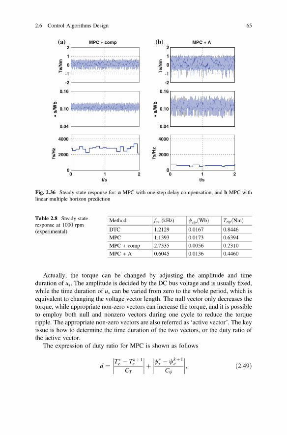
Figures 2.35 and 2.36 show the measured steady-state performance at 1000 rpm.It is seen that the implementation of MPC can reduce the torque ripple, but does notreduce the flux ripple. When the one-step delay is compensated, a significantdecrease of torque and flux ripples can be found as well as an obvious increase ofswitching frequency. When the linear multiple horizon prediction is added to MPC,it can be seen that the torque and flux ripples are slightly decreased along with alimited reduction of the switching frequency.

Table 2.8 lists the torque and flux ripples of these control methods in experiment.As shown, similar conclusions can be obtained as those from Table 2.7. Accordingto the analysis above, it can be concluded that:

(1) MPC can achieve lower torque ripple than that of DTC whilstmaintaining/reducing the switching frequency as proven in both simulationand experimental tests. However, MPC’s ability in flux ripple reduction isinsignificant and even unstable.

0246

Te/

Nm

0.1

0.150.2

0.05

Ph

i/Wb

0 0.1 0.2 0.3 0.4 0.50

2000

4000

t/s

fs/H

z

-10

0

10

ia/A

MPC + comp

0500

100015002000

Sp

eed

/rp

m

Fig. 2.31 Combined load testfor MPC with one-step delaycompensation


(2) When one-step delay is compensated, the steady-state performance of MPC interms of torque and flux ripples reduction is significantly improved. It shouldbe noticed that the performance improvement also comes with a remarkableswitching frequency increase (two times or more).

(3) By introducing linear multiple horizon prediction to MPCs, a significantswitching frequency reduction can be found as well as an obvious decrease influx ripple. However, it comes with heavy penalty of torque ripple increasing,especially at low motor speed.

0246

Te/

Nm

0.1

0.150.2

0.05

Ph

i/Wb

0 0.1 0.2 0.3 0.4 0.50

2000

4000

t/s

fs/H

z

-10

0

10

ia/A

MPC + A

0500

100015002000

Sp

eed

/rp

m

Fig. 2.32 Combined load testfor MPC with linear multiplehorizon prediction

Table 2.7 Steady-stateresponse (simulation)

Method THD(%)

fav(kHz)

wripðWbÞ TripðNmÞ

DTC 28.83 1.5972 0.0155 0.6869

MPC 18.55 1.5692 0.0138 0.4952

MPC + comp 8.17 1.5812 0.0059 0.2253

MPC + A 15.52 0.6640 0.0090 0.5102


2.6.6 Improved MPC with Duty Ratio Optimization

There are many improvements for these control algorithms. One of them known asMPC with duty ratio optimization will be selected for the control of PM-SMCTFM. As a general algorithm, the theory and test results will be presented in thissection.

Fig. 2.33 Experimental setup of testing system: a overview of the testing platform and b frontview of the PMSM and inverter control board


In the conventional MPC, the selected voltage vector works during the wholesampling period. In many cases, it is not necessary to work for the entire period tomeet the performance requirement of torque and flux. This is one of the mainreasons for the torque and flux ripples. By introducing a null vector to each sam-pling period, the effects of voltage on torque can be adjusted to be more moderate,in order to diminish the ripples of torque and flux.

Fig. 2.34 Dynamo-meter controller DSP6000

-2

-1

0

1

2

Te/

Nm

Classic DTC(a) (b)

0.04

0.10

0.16

• s/

Wb

0 1 20

2000

4000

t/s

fs/H

z

-2

-1

0

1

2

Te/

Nm

MPC

0.04

0.10

0.16

• s/

Wb

0 1 20

2000

4000

t/s

fs/H

z

Fig. 2.35 Steady-state response for: a DTC, b MPC


Actually, the torque can be changed by adjusting the amplitude and timeduration of us. The amplitude is decided by the DC bus voltage and is usually fixed,while the time duration of us can be varied from zero to the whole period, which isequivalent to changing the voltage vector length. The null vector only decreases thetorque, while appropriate non-zero vectors can increase the torque, and it is possibleto employ both null and nonzero vectors during one cycle to reduce the torqueripple. The appropriate non-zero vectors are also referred as ‘active vector’. The keyissue is how to determine the time duration of the two vectors, or the duty ratio ofthe active vector.

The expression of duty ratio for MPC is shown as follows

d ¼ T�e � Tkþ 1

e

CT

��þ w�

s � wkþ 1e

Cw

��; ð2:49Þ

-2

-1

0

1

2

Te/

Nm

MPC + comp(a) (b)

0.04

0.10

0.16

• s/

Wb

0 1 20

2000

4000

t/s

fs/H

z

-2

-1

0

1

2

Te/

Nm

MPC + A

0.04

0.10

0.16

• s/

Wb

0 1 20

2000

4000

t/s

fs/H

z

Fig. 2.36 Steady-state response for: a MPC with one-step delay compensation, and b MPC withlinear multiple horizon prediction

Table 2.8 Steady-stateresponse at 1000 rpm(experimental)

Method fav (kHz) wripðWbÞ TripðNmÞDTC 1.2129 0.0167 0.8446

MPC 1.1393 0.0173 0.6394

MPC + comp 2.7335 0.0056 0.2310

MPC + A 0.6045 0.0136 0.4460


where d is the duty ratio of the active voltage vector, and CT and Cψ are twopositive parameters. The idea of this method is that the larger the difference betweenthe reference and predicted torque values, the larger is the duty ratio value [36]. Onthe other hand, the lower the CT and Cψ values, the quicker is the dynamic response(e.g. take less time to reach the given speed), but the poorer will be the steady-stateresponse (e.g. higher torque and flux ripples). Higher values of CT and Cψ couldlead to better steady-state responses, but slower dynamic responses. Therefore, thedetermination of these values is a compromise between the steady-state anddynamic performances. Extensive simulation and experimental results have proventhat the PM flux value and half-rated torque value for CT and Cψ can provide a goodcompromise between the steady state performance and the dynamic response. Theblock diagram of the proposed improved MPC is shown in Fig. 2.37.

2.6.7 Numerical and Experimental Comparisons of DTCand MPC with Duty Ratio Optimization

2.6.7.1 Numerical Simulation

The parameters of the motor and control system simulated in this section are listedin Table 2.9. Similar to the previous test example, this simulation test combines thestart-up, steady-state and external load tests. The motor starts up from 0 s withseveral reference speeds (500 rev/min, 1000 rev/min, 1500 rev/min and 2000rev/min). After reaching the reference speed, the motor maintains the speed for atleast 0.2 s and an external load is applied at 0.3 s. Figure 2.38 shows the combinedload test for one reference speed, 1000 rev/min. From top to bottom, the curves are

Fig. 2.37 Diagram of an improved MPC with duty ratio optimization in MATLAB/SIMULINK


the stator current, stator flux, torque, motor speed, and switching frequency,respectively. The test results for other speed situations can be found in [36].

It can be found that the proposed MPC scheme present very low torque and fluxripples and excellent dynamic response. The proposed MPC scheme also presentsvery low stator current THDs and narrow harmonic spectrums with the dominantharmonics of around 5 kHz.

Table 2.9 Motor and controlsystem parameters

Parameter Symbol Value

Number of pole pairs p 3

Permanent magnet flux wf 0.1057 Wb

Stator resistance Rs 1.8 Ω

d-axis and q-axis inductance Ld, Lq 15 mH

DC bus voltage Vdc 200 V

Inertia J 0.002 kg �m2

Torque constant gain CT 2

Flux constant gain Cw 0.1

Sampling frequency fsp 5 kHz

0

2

4

6

Te/

Nm

0.1

0.15

0.2

0.05

Ph

i/Wb

0 0.1 0.2 0.3 0.4 0.50

2000

4000

6000

t/s

fs/H

z

-10

0

10

ia/A

MPC + Duty

0500

100015002000

Sp

eed

/rp

m

0

0.5

1

Du

ty

Fig. 2.38 Combined load testfor MPC with duty ratiooptimization at 1000 rev/min


2.6.7.2 Experimental Test

The experimental tests are performed on the same testing platform introduced in thelast section. Figure 2.39 shows the steady-state responses at 1000 rpm for threecontrol strategies, namely (a) DTC, (b) MPC, and (c) MPC with duty ratiooptimization.

0 1 20

2000

4000

t/s

fs/H

z

0.04

0.10

0.16

Ph

is/W

b

-2

-1

0

1

2

Te/

Nm

MPC

0 1 20

2000

4000

t/s

fs/H

z

0.04

0.10

0.16

Ph

is/W

b

-2

-1

0

1

2

Te/

Nm

Classic DTC(a) (b)

(c)

-2

-1

0

1

2

Te/

Nm

MPC Duty

0.04

0.10

0.16

Ph

is/W

b

0

2000

4000

fs/H

z

0 1 20

0.5

1

t/s

du

ty

Fig. 2.39 Steady-state response at 1000 rpm for: a DTC, b MPC and c MPC with duty ratiooptimization


It can be seen that in MPC with duty ratio optimization, the torque and fluxripples are reduced significantly compared to other methods. The duty ratioincreases along with the increase in motor speed.

According to the analysis above, it can be concluded that:

(1) MPC with duty ratio optimization can achieve a better performance than DTCand original MPC in terms of torque and flux ripples reduction;

(2) Under the same system sampling frequency (5 kHz), the switching frequencyof the improved method is much higher than other methods; and

(3) In DTC and MPC, the switching frequency slightly decreases along with theincrease of motor speed. However, the switching frequency is almost stable inthe proposed method.

More experimental results including different speed, dynamic response and dataanalysis can be found in [36].

2.7 Summary

This chapter presents the multi-disciplinary design analysis models and methods forelectrical machines and drive systems. All the models and methods are discussed interms of the three major parts of electrical drive systems, namely electricalmachines, power electronic converters and controllers. Electromagnetic, thermaland mechanical analyses based on different models, e.g. FEM, have been investi-gated for the design of electrical machines with several prototypes developed in ourresearch center. Various kinds of popular control algorithms have been describedfor the controller design. Several examples investigated in our previous work havebeen presented to show the effectiveness of the proposed models and analysismethods.

References

1. Lei G, Wang TS, Guo YG, Zhu JG, Wang SH (2014) System level design optimizationmethods for electrical drive systems: deterministic approach. IEEE Trans Ind Electron 61(12):6591–6602

2. Lei G, Wang TS, Zhu JG, Guo YG, Wang SH (2015) System level design optimizationmethod for electrical drive system: robust approach. IEEE Trans Ind Electron 62(8):4702–4713

3. Zhu JG, Guo YG, Lin ZW, Li YJ, Huang YK (2011) Development of PM transverse fluxmotors with soft magnetic composite cores. IEEE Trans Magn 47(10):4376–4383

4. Zhu JG, Ramsden VS (1998) Improved formulations for rotational core losses in rotatingelectrical machines. IEEE Trans Magn 34(4):2234–2242

5. Guo YG, Zhu JG, Lu HY, Lin ZW, Li YJ (2012) Core loss calculation for soft magneticcomposite electrical machines. IEEE Trans Magn 48(11):3112–3115


6. Guo YG, Zhu JG, Lu HY, Li YJ, Jin JX (2014) Core loss computation in a permanent magnettransverse flux motor with rotating fluxes. IEEE Trans Magn 50(11). Article#: 6301004

7. Guo YG, Zhu JG, Zhong JJ, Wu W (2003) Core losses in claw pole permanent magnetmachines with soft magnetic composite stators. IEEE Trans Magn 39(5):3199–3201

8. Huang YK, Zhu JG, Guo YG, Lin ZW, Hu Q (2007) Design and analysis of a high speed clawpole motor with soft magnetic composite core. IEEE Trans Magn 43(6):2492–2494

9. Huang YK, Zhu JG et al (2009) Thermal analysis of high-speed SMC motor based on thermalnetwork and 3-D FEA with rotational core loss included. IEEE Trans Magn 45(10):4680–4683

10. Pfister P-D, Perriard Y (2010) Very-high-speed slotless permanent-magnet motors: analyticalmodeling, optimization, design, and torque measurement methods. IEEE Trans Ind Electron57(1):296–303

11. Komeza K, Dems M (2012) Finite-element and analytical calculations of no-load core lossesin energy-saving induction motors. IEEE Trans Ind Electron 59(7):2934–2946

12. Wang SH, Meng XJ, Guo NN, Li HB, Qiu J, Zhu JG et al (2009) Multilevel optimization forsurface mounted PM machine incorporating with FEM. IEEE Trans Magn 45(10):4700–4703

13. Barcaro M, Bianchi N, Magnussen F (2012) Permanent-magnet optimization inpermanent-magnet-assisted synchronous reluctance motor for a wide constant-power speedrange. IEEE Trans Ind Electron 59(6):2495–2502

14. Vese I, Marignetti F, Radulescu MM (2010) Multiphysics approach to numerical modeling ofa permanent-magnet tubular linear motor. IEEE Trans Ind Electron 57(1):320–326

15. Bornschlegell AS, Pelle J, Harmand S, Fasquelle A, Corriou J-P (2013) Thermal optimizationof a high-power salient-pole electrical machine. IEEE Trans Ind Electron 60(5):1734–1746

16. Lee D-H, Pham TH, Ahn J-W (2013) Design and operation characteristics of four-two polehigh-speed SRM for torque ripple reduction. IEEE Trans Ind Electron 60(9):3637–3643

17. Flieller D, Nguyen NK, Wira P, Sturtzer G, Abdeslam DO, Merckle J (2014) A self-learningsolution for torque ripple reduction for nonsinusoidal permanent-magnet motor drives basedon artificial neural networks. IEEE Trans Ind Electron 61(2):655–666

18. Hasanien HM, Abd-Rabou AS, Sakr SM (2010) Design optimization of transverse flux linearmotor for weight reduction and performance improvement using response surfacemethodology and genetic algorithms. IEEE Trans Energy Convers 25(3):598–605

19. Hasanien HM (2011) Particle swarm design optimization of transverse flux linear motor forweight reduction and improvement of thrust force. IEEE Trans Ind Electron 58(9):4048–4056

20. Lei G, Liu CC, Guo YG, Zhu JG (2015) Multidisciplinary design analysis for PM motors withsoft magnetic composite cores. IEEE Trans Magn 51(11). Article 8109704

21. Hua W, Cheng M, Zhu ZQ, Howe D (2006) Design of flux-switching permanent magnetmachine considering the limitation of inverter and flux-weakening capability. In: Proceedingsof 41st IAS annual meeting-industry applications conference, vol 5, pp 2403–2410

22. Liu CC, Zhu JG, Wang YH, Lei G, Guo YG, Liu XY (2014) A low-cost permanent magnetsynchronous motor with SMC and ferrite PM. In: Proceedings of 17th international conferenceon electrical machines and systems (ICEMS), pp 397–400

23. Fei W, Luk PCK, Shen JX, Wang Y, Jin M (2012) A novel permanent-magnet flux switchingmachine with an outer-rotor configuration for in-wheel light traction applications. IEEE TransInd Appl 48(5):1496–1506

24. Guo YG (2003) Development of low cost high performance permanent magnet motors usingnew soft magnetic composite materials, UTS thesis (PhD)

25. Guo YG, Zhu JG, Watterson PA, Wei Wu (2006) Development of a PM transverse flux motorwith soft magnetic composite core. IEEE Trans Energy Conver 21(2):426–434

26. Guo YG, Zhu JG, Watterson PA, Wei Wu (2003) Comparative study of 3-D flux electricalmachines with soft magnetic composite cores. IEEE Trans Ind Appl 39(6):1696–1703

27. Guo YG, Zhu JG, Dorrell D (2009) Design and analysis of a claw pole PM motor with moldedSMC core. IEEE Trans Magn 45(10):582–4585

28. Lei G, Shao KR, Guo YG, Zhu JG (2012) Multi-objective sequential optimization method forthe design of industrial electromagnetic devices. IEEE Trans Magn 48(11):4538–4541


29. Lei G, Guo YG, Zhu JG et al (2012) System level six sigma robust optimization of a drivesystem with PM transverse flux machine. IEEE Trans Magn 48(2):923–926

30. Lei G, Zhu JG, Guo YG, Hu JF, Xu W, Shao KR (2013) Robust design optimization ofPM-SMC motors for Six Sigma quality manufacturing. IEEE Trans Magn 49(7):3953–3956

31. Lei G, Zhu JG, Guo YG, Shao KR, Xu W (2014) Multiobjective sequential designoptimization of PM-SMC motors for six sigma quality manufacturing. IEEE Trans Magn, 50(2). Article 7017704

32. Liu CC, Zhu JG, Wang YH, Guo YG, Lei G, Liu XY (2015) Development of a low-costdouble rotor axial flux motor with soft magnetic composite and ferrite permanent magnetmaterials. J Appl Phys, 117(17). Article # 17B507

33. Teng QF, Zhu JG, Wang TS, Lei G (2012) Fault tolerant direct torque control of three-phasepermanent magnet synchronous motors. WSEAS Trans Syst 8(11):465–476

34. Teng QF, Bai J, Zhu JG, Sun Y (2013) Fault tolerant model predictive control of three-phasepermanent magnet synchronous motors. WSEAS Trans Syst 12(8):385–397

35. Wang Y (2011) Investigation of rotor position detection schemes for PMSM drives based onanalytical machine model incorporating nonlinear saliencies, UTS thesis (PhD)

36. Wang TS (2013) Model predictive torque control of PMSM with duty ratio optimization fortorque ripple reduction, UTS thesis (Master degree)

37. Kim SY, Lee W, Rho MS, Park SY (2010) Effective dead-time compensation using a simplevectorial disturbance estimator in PMSM drives. IEEE Trans Ind Electron 57(5):1609–1614

38. Lee J, Hong J, Nam K, Ortega R, Praly L, Astolfi A (2010) Sensorless control ofsurface-mount permanent-magnet synchronous motors based on a nonlinear observer. IEEETrans Power Electron 25(2):290–297

39. Genduso F, Miceli R, Rando C, Galluzzo GR (2010) Back EMF sensorless-control algorithmfor high-dynamic performance PMSM. IEEE Trans Ind Electron 57(6):2092–2100

40. Takahashi I, Noguchi T (1986) A new quick-response and high-efficiency control strategy ofan induction motor. IEEE Trans Ind Appl 22(5):820–827

41. Depenbrock M (1988) Direct self-control (DSC) of inverter-fed induction machine. IEEETrans Power Electron 3(4):420–429

42. Buja GS, Kazmierkowski MP (2004) Direct torque control of PWM inverter-fed AC motors-Asurvey. IEEE Trans Ind Electron 51(4):744–757

43. Lai YS, Chen JH (2001) A new approach to direct torque control of induction motor drives forconstant inverter switching frequency and torque ripple reduction. IEEE Trans EnergyConvers 16(3):220–227

44. Lascu C, Trzynadlowski A (2004) A sensorless hybrid DTC drive for high-volume low-costapplications. IEEE Trans Ind Electron 51(5):1048–1055

45. Zhang Y, Zhu J, Xu W, Hu J, Dorrell DG, Zhao Z (2010) Speed sensorless stator flux orientedcontrol of three-level inverter-fed induction motor drive based on fuzzy logic and sliding modecontrol. In: Proceedings of 36th IEEE IECON, pp 2926–293

46. Zhang Y, Zhu J (2011) Direct torque control of permanent magnet synchronous motor withreduced torque ripple and commutation frequency. IEEE Trans Power Electron 26(1):235–248

47. Zhang Y, Zhu J (2011) A novel duty cycle control strategy to reduce both torque and fluxripples for DTC of permanent magnet synchronous motor drives with switching frequencyreduction. IEEE Trans Power Electron 26(10):3055–3067

48. Zhang Y, Zhu J, Xu W, Guo Y (2011) A simple method to reduce torque ripple in directtorque-controlled permanent-magnet synchronous motor by using vectors with variableamplitude and angle. IEEE Trans Ind Electron 58(7):2848–2859

49. Wang TS, Zhu JG, Zhang YC (2011) Model predictive torque control for PMSM with dutyratio optimization. In Proceedings of 2011 international conference on electrical machines andsystems (ICEMS), pp 1–5, 20–23 August 2011

50. Miranda H, Cortes P, Yuz J, Rodriguez J (2009) Predictive torque control of inductionmachines based on state-space models. IEEE Trans Ind Electron 56(6):1916–1924

51. Geyer T, Papafotiou G, Morari M (2009) Model predictive direct torque control—Part I:Concept, algorithm, and analysis. IEEE Trans Ind Electron 56(6):1894–1905

References 71

52. Kouro S, Cortes P, Vargas R, Ammann U, Rodriguez J (2009) Model predictive control—asimple and powerful method to control power converters. IEEE Trans Ind Electron 56(6):1826–1838

53. Morel F, Retif J-M, Lin-Shi X, Valentin C (2008) Permanent magnet synchronous machinehybrid torque control. IEEE Trans Ind Electron 55(2):501–511

54. Drobnic K, Nemec M, Nedeljkovic D, Ambrozic V (2009) Predictive direct control applied toAC drives and active power filter. IEEE Trans Ind Electron 56(6):1884–1893

55. Zhang Y, Xie W (2014) Low complexity model predictive control-single vector-basedapproach. IEEE Trans Power Electron 29(10):5532–5541

56. Zhang Y, Qu C (2015) Model predictive direct power control of PWM rectifiers underunbalanced network conditions. IEEE Trans Ind Electron 62(7):4011–4022


http://www.springer.com/978-3-662-49269-7

design fundamentals of electrical machines and drive systems

Documents