design, implementation, and evaluation of an …stevedh/pubs/mthesis.pdfdesign, implementation, and...
TRANSCRIPT
Design, Implementation, and Evaluation of an Embedded IPv6 Stack
by
Stephen Dawson-Haggerty
A.B. Harvard University 2007
A thesis submitted in partial satisfactionof the requirements for the degree of
Master of Science
in
Computer Science – Electrical Engineering and Computer Sciences
in the
GRADUATE DIVISION
of the
UNIVERSITY OF CALIFORNIA, BERKELEY
Committee in charge:
David Culler, ChairKris Pister
Spring 2010

The thesis of Stephen Dawson-Haggerty is approved.
Chair Date
Date
University of California, Berkeley
Spring 2010

iii
Abstract
Design, Implementation, and Evaluation of an Embedded IPv6 Stack
by
Stephen Dawson-Haggerty
Master of Science in Computer Science – Electrical Engineering and Computer Sciences
University of California, Berkeley
David Culler, Chair
In this thesis, we present blip, an IPv6 stack for embedded devices, and report on using it to
develop a new routing protocol, Hydro, and a deployment of an energy monitoring system.
Because of the constrained nature of the devices used in many sensor networks, it is a challenge
to provide high-level networking abstractions while remaining efficient. We discuss building on
previous work by Hui and ongoing discussions in standards bodies to produce a stack which sup-
ports embedded operation. We propose Hydro, a new routing protocol which efficiently supports
the common many-to-one “collection” traffic pattern, while adding the ability to short-cut point-
to-point routes in the network. We found that this protocol can support this type of any-to-any
communication better then existing routing solutions when measured by control overhead.
Finally we examine a real application problem: plug-load energy metering. Using the ACme
platform, we discuss experiences using blip in a pilot deployment of about 50 plug-load electricity
meters in a Computer Science lab.
David CullerThesis Committee Chair
1
Contents
Contents i
Acknowledgements iv
1 Introduction 1
2 The BLIP IPv6 Stack 3
2.1 Overview . . . . . . . . . . . . . . . . . . . . . . . . . . . . . . . . . . . . . . . 3
2.2 The 6lowpan Layer . . . . . . . . . . . . . . . . . . . . . . . . . . . . . . . . . 4
2.2.1 Upper 6lowpan Interface . . . . . . . . . . . . . . . . . . . . . . . . . . 4
2.3 Network Layer . . . . . . . . . . . . . . . . . . . . . . . . . . . . . . . . . . . . 5
2.3.1 Route Over . . . . . . . . . . . . . . . . . . . . . . . . . . . . . . . . . . 6
2.3.2 Addressing . . . . . . . . . . . . . . . . . . . . . . . . . . . . . . . . . . 6
2.3.3 IPv6 Configuration Mechanisms . . . . . . . . . . . . . . . . . . . . . . . 8
2.3.4 Extension Mechanisms . . . . . . . . . . . . . . . . . . . . . . . . . . . . 8
2.4 Transport Protocols . . . . . . . . . . . . . . . . . . . . . . . . . . . . . . . . . . 9
2.4.1 UDP . . . . . . . . . . . . . . . . . . . . . . . . . . . . . . . . . . . . . 10
2.4.2 TCP . . . . . . . . . . . . . . . . . . . . . . . . . . . . . . . . . . . . . . 10
2.5 Tools . . . . . . . . . . . . . . . . . . . . . . . . . . . . . . . . . . . . . . . . . . 12
3 The Hydro Routing Protocol 14
3.1 Overview . . . . . . . . . . . . . . . . . . . . . . . . . . . . . . . . . . . . . . . 14
3.2 Background . . . . . . . . . . . . . . . . . . . . . . . . . . . . . . . . . . . . . . 16
3.2.1 Existing Low-Power Protocols . . . . . . . . . . . . . . . . . . . . . . . . 16
3.2.2 Ad-Hoc Networking Protocols . . . . . . . . . . . . . . . . . . . . . . . . 18
3.2.3 Internet Solutions . . . . . . . . . . . . . . . . . . . . . . . . . . . . . . . 19
i
3.2.4 Towards a Hybrid Solution . . . . . . . . . . . . . . . . . . . . . . . . . . 20
3.3 Hydro Design and Operation . . . . . . . . . . . . . . . . . . . . . . . . . . . . . 21
3.3.1 Distributed DAG formation . . . . . . . . . . . . . . . . . . . . . . . . . 21
3.3.2 Global Topology Construction . . . . . . . . . . . . . . . . . . . . . . . . 24
3.3.3 Centralized Route Installation . . . . . . . . . . . . . . . . . . . . . . . . 25
3.3.4 Forwarding . . . . . . . . . . . . . . . . . . . . . . . . . . . . . . . . . . 26
3.3.5 Multiple Border Routers . . . . . . . . . . . . . . . . . . . . . . . . . . . 28
3.3.6 State Management . . . . . . . . . . . . . . . . . . . . . . . . . . . . . . 29
3.4 Evaluation . . . . . . . . . . . . . . . . . . . . . . . . . . . . . . . . . . . . . . . 30
3.4.1 Metrics . . . . . . . . . . . . . . . . . . . . . . . . . . . . . . . . . . . . 30
3.4.2 Methodology . . . . . . . . . . . . . . . . . . . . . . . . . . . . . . . . . 31
3.4.3 Implementation Details . . . . . . . . . . . . . . . . . . . . . . . . . . . . 31
3.4.4 Distributed DAG Formation . . . . . . . . . . . . . . . . . . . . . . . . . 32
3.4.5 Global Topology View . . . . . . . . . . . . . . . . . . . . . . . . . . . . 32
3.4.6 Centralized Route Installation . . . . . . . . . . . . . . . . . . . . . . . . 35
3.4.7 Scalability . . . . . . . . . . . . . . . . . . . . . . . . . . . . . . . . . . 41
3.4.8 Footprint and Overhead Analysis . . . . . . . . . . . . . . . . . . . . . . 42
3.4.9 IETF Criteria . . . . . . . . . . . . . . . . . . . . . . . . . . . . . . . . . 44
3.5 Extensions and Future Work . . . . . . . . . . . . . . . . . . . . . . . . . . . . . 45
3.5.1 Multicast Forwarding . . . . . . . . . . . . . . . . . . . . . . . . . . . . . 45
3.5.2 Policy-Based Routing . . . . . . . . . . . . . . . . . . . . . . . . . . . . 45
3.6 Limitations . . . . . . . . . . . . . . . . . . . . . . . . . . . . . . . . . . . . . . 46
3.6.1 Adapting to Dynamic Topologies . . . . . . . . . . . . . . . . . . . . . . 46
3.6.2 Source-Routing in Deep Networks . . . . . . . . . . . . . . . . . . . . . . 46
3.6.3 Single Point of Congestion/Failure . . . . . . . . . . . . . . . . . . . . . . 47
4 Example Deployemnt: AC Metering 48
4.1 Overview . . . . . . . . . . . . . . . . . . . . . . . . . . . . . . . . . . . . . . . 48
4.2 System Architecture . . . . . . . . . . . . . . . . . . . . . . . . . . . . . . . . . . 50
4.3 ACme Network . . . . . . . . . . . . . . . . . . . . . . . . . . . . . . . . . . . . 51
4.3.1 Edge Router . . . . . . . . . . . . . . . . . . . . . . . . . . . . . . . . . 52
4.3.2 Transport . . . . . . . . . . . . . . . . . . . . . . . . . . . . . . . . . . . 52
4.3.3 Network Performance . . . . . . . . . . . . . . . . . . . . . . . . . . . . 53
4.4 ACme Application Tier . . . . . . . . . . . . . . . . . . . . . . . . . . . . . . . . 54
ii

4.5 Related Work . . . . . . . . . . . . . . . . . . . . . . . . . . . . . . . . . . . . . 55
4.6 Discussion . . . . . . . . . . . . . . . . . . . . . . . . . . . . . . . . . . . . . . . 56
5 Conclusions 58
Bibliography 60
References . . . . . . . . . . . . . . . . . . . . . . . . . . . . . . . . . . . . . . . . . . 60
iii
Acknowledgements
This work has benefited from many invaluable collaborations, inside and outside of Berkeley. I
will attempt to thank everyone who has had a hand in moving blip out into the world.
First, thanks to Jonathan Hui for the intellectual framework that the work rests on, and for giving
the academic community the kick it needed to move forward. To Prabal Dutta, thanks for many
useful conversations about everything, and especially for noticing that Backcast actually works;
A-MAC could not have been possible without it. Thanks to Arsalan Tavakoli for many fruitful
design conversations about Hydro and implementation help. Experiments with Jorge Ortiz helped
to improve my understanding of the dynamics of low-power wireless links. To Jorge Ortiz, Xiaofan
Jiang, and Jay Taneja of Berkeley, Tim Wark of CSIRO, and Noritaka Matsumoto of Hitachi, thanks
for biting the bullet, diving in, and using blip on your own projects. The up-close, real-world
feedback was invaluable.
Thanks to Jeongil Ko of Johns Hopkins for helping to develop and flesh out the interface to the
routing layer for blip-2.0 in the course of developing a RPL implementation.
I owe a debt to Phil Levis and Omprakash Gawaldi for shepherding the TinyOS distribution
and helping to beat blip into shape for the 2.1.1 release (maybe someday there will even be a
Windows version!); also for the learning experience that was producing the IETF protocol survey
draft. Thanks to Miklos Maroti for helpful discussions about the interface to the link layer, and
implementing the result of these discussions for the RF230 radio. Finally, thanks for all the useful
feedback, patches, and encouragement from the modest community which has formed around this
project.
My adviser, David Culler has provided encouragement and support at every step, and has always
pushed to make it more real and actually use it. Also, I have to thank my undergraduate adviser Matt
Welsh the bit of advice “if you’re not sure what to do, just start building something”.
Finally, my parents provided my first model of the academic lifestyle by bringing me to Cafe
Strada at the tender age of ten days; important lessons start early.
iv

v
Chapter 1
Introduction
As wireless sensor networks move from the lab and the academy into the real world, much of
their future direction is in the hands of industrial standards bodies which will specifiy how to make
them reliable, low-power, and interoperable. In particular, it has become increasingly clear in the
past two years that IPv6 will play a central role in this future architecture. Open-source is a key
enabler for timely, relevent academic research because most groups and institutions do not have the
resources to implement the full set of standards. TinyOS has served this role well, by providing a
proven software base for academic research. However, we saw a gap in 2008 in its offerings as much
of the world migrated to the IP architecture. Publications like Hui’s elucidation of a complete IP
architecture for embedded devices did much to raise the visibility of this approach within academia
while various working groups in the Internet Engineering Task Force gained a growing amount of
industrial support. However, there was no open effort to bring the IP architecture to TinyOS.
The solution, following the Berkeley tradition of open software, was to kick off an implementa-
tion effort for b6lowPAN, the Berkeley 6lowPAN stack – later renamed blip. Since then, blip
has progressed through six public releases, acquiring many bells and whistles along the way. At
present, blip is in transition to version 2.0 which will include support for the latest IETF stan-
dards; there are 70 users at 38 unique domains worldwide on the project mailing list.
In addition to serving an important community function, blip also has become the base soft-
ware stack for projects within the Berkeley Wireless and Embedded Systems lab. We have deployed
1
hundreds of devices using it to monitor environmental conditions and electic power consumption,
and are in the process of deploying hundreds more, in collaboration with Lawrence Berkeley Na-
tional Laboratory. Furthermore, blip has served as a research platform for research into media
access and routing protocols, some of which is presented in this thesis. It will be an essential
enabling technology of the “Building Operating-system” that is the current focus of our research
group.
There are three main contributions of this thesis. First, we present our open implementation of
the IPv6 architecture for embedded devices, the blip IPv6 stack. In doing so, we accept the archi-
tecture presented by Hui and more fully explore the design space posed by this layered architecture.
Secondly, we propose Hydro, a routing protocol for resource-constrained devices which leverages
the existing heirarchy of device capabilities in today’s networks. Finally, we conclude with a few
notes on an actual deployment of blip in an electric power metering application.
2
Chapter 2
The BLIP IPv6 Stack
2.1 Overview
To enable research explorations within the IP architecture, we have implemented much of the
architecture developed by the IETF and explained by Hui [1], [2]. This part of the work broke only
a moderate amount of new ground, but has proven to be an important research enabler, in more ways
then one. Thus, we confine our discussion to a survey of the overall structure of the stack and some
important details, leaving a more complete treatment to technical documentation.
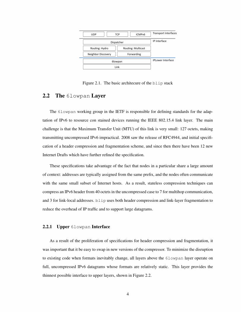
The core of the blip IPv6 stack consists of three layers:
6lowpan The 6lowpan layer provides a “layer 2.5” abstraction on top of the link layer. It com-
presses certain higher-level headers and breaks large packets into multiple link-layer frag-
ments. This layer sits on top of multiple link layers.
Network blip uses a routing protocol called Hydro to provide unicast reachability within a sub-
network of IPv6 devices. Described in more detail in the next chapter, Hydro builds a routing
gradient towards a subset of egress routers.
Transport Two standard Internet transport protocols are included with blip: the User Datagram
Protocol (UDP) and the Transport Control Protocol (TCP).
3
!"#$%
&'()*+#%
,-.% /0.% 102.3&%
4(56#78%9:;<(% 4(56#78%25'6=+>?%
@A"7BC(<%-">=(3A<:% D(<)+<;"#7%
-">*+?=BA<%
1.!()A<%1#?A<E+=A%
1.%1#?A<E+=A%
/<+#>*(<?%1#?A<E+=A>%
Figure 2.1. The basic architecure of the blip stack
2.2 The 6lowpan Layer
The 6lowpan working group in the IETF is responsible for defining standards for the adap-
tation of IPv6 to resource con stained devices running the IEEE 802.15.4 link layer. The main
challenge is that the Maximum Transfer Unit (MTU) of this link is very small: 127 octets, making
transmitting uncompressed IPv6 impractical. 2008 saw the release of RFC4944, and initial specifi-
cation of a header compression and fragmentation scheme, and since then there have been 12 new
Internet Drafts which have further refined the specification.
These specifications take advantage of the fact that nodes in a particular share a large amount
of context: addresses are typically assigned from the same prefix, and the nodes often communicate
with the same small subset of Internet hosts. As a result, stateless compression techniques can
compress an IPv6 header from 40 octets in the uncompressed case to 7 for multihop communication,
and 3 for link-local addresses. blip uses both header compression and link-layer fragmentation to
reduce the overhead of IP traffic and to support large datagrams.
2.2.1 Upper 6lowpan Interface
As a result of the proliferation of specifications for header compression and fragmentation, it
was important that it be easy to swap in new versions of the compressor. To minimize the disruption
to existing code when formats inevitably change, all layers above the 6lowpan layer operate on
full, uncompressed IPv6 datagrams whose formats are relatively static. This layer provides the
thinnest possible interface to upper layers, shown in Figure 2.2.
4
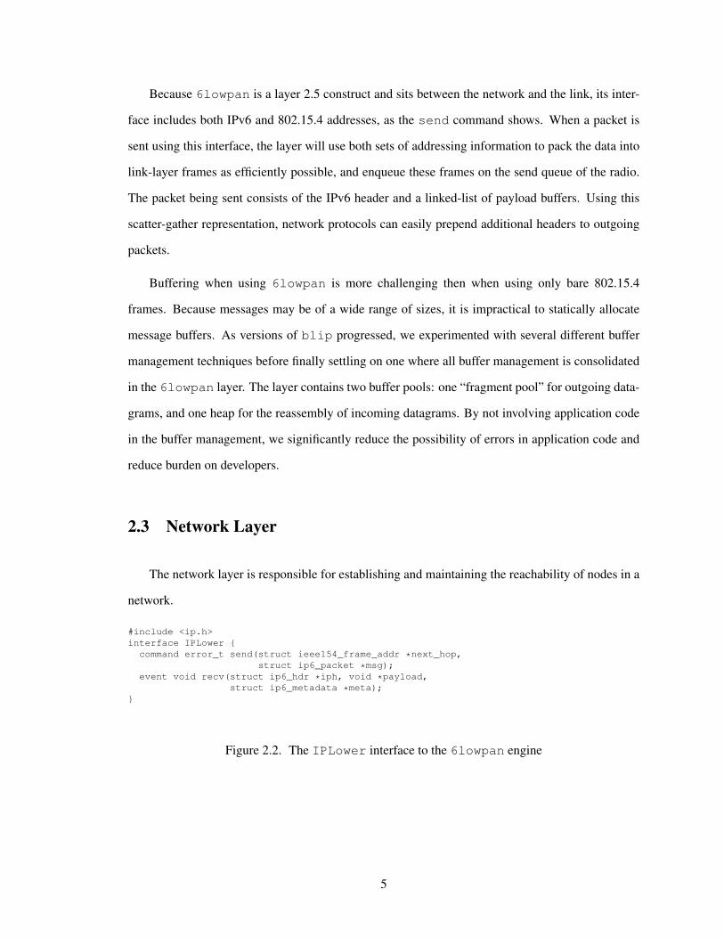
Because 6lowpan is a layer 2.5 construct and sits between the network and the link, its inter-
face includes both IPv6 and 802.15.4 addresses, as the send command shows. When a packet is
sent using this interface, the layer will use both sets of addressing information to pack the data into
link-layer frames as efficiently possible, and enqueue these frames on the send queue of the radio.
The packet being sent consists of the IPv6 header and a linked-list of payload buffers. Using this
scatter-gather representation, network protocols can easily prepend additional headers to outgoing
packets.
Buffering when using 6lowpan is more challenging then when using only bare 802.15.4
frames. Because messages may be of a wide range of sizes, it is impractical to statically allocate
message buffers. As versions of blip progressed, we experimented with several different buffer
management techniques before finally settling on one where all buffer management is consolidated
in the 6lowpan layer. The layer contains two buffer pools: one “fragment pool” for outgoing data-
grams, and one heap for the reassembly of incoming datagrams. By not involving application code
in the buffer management, we significantly reduce the possibility of errors in application code and
reduce burden on developers.
2.3 Network Layer
The network layer is responsible for establishing and maintaining the reachability of nodes in a
network.
#include <ip.h>interface IPLower {
command error_t send(struct ieee154_frame_addr *next_hop,struct ip6_packet *msg);
event void recv(struct ip6_hdr *iph, void *payload,struct ip6_metadata *meta);
}
Figure 2.2. The IPLower interface to the 6lowpan engine
5
2.3.1 Route Over
A central question for implementing IPv6 in sensor networks is what has become know as
“route over” vs. “mesh under” in the IETF. In mesh under networking, routing is done on layer two
addresses, and every host is one hop from every other. Although this is the most compatible with
existing assumptions about subnet design, it leads to significant redundancies and inefficiencies in
this space. The alternative, so called route-over exposes the radio topology at the IP layer. While
not compatible with some IPv6 mechanisms, this is becoming the favored approach since a single
set of tools can be used to debug networks.
There are a number of existing routing protocols for IPv6, some targeted at wireless links.
However, IPv6 itself does not require any particular routing protocol to be used with a domain;
common choices in wired networks are OSPF and IS-IS [3], [4]. As part of this thesis work, we
developed a set of criteria for benchmarking existing protocols, and concluded that no existing
protocol is appropriate for this space [5]. Existing protocols with TinyOS implementations such
as DYMO or S4 may be appropriate for this task [6], [7]; collection and dissemination protocols
like CTP or Drip are probably not directly applicable since they are address-free although their
underlying mechanisms of tree formation and efficient broadcast are extremely relevant [8], [9].
blip takes the route-over approach, and uses the Hydro routing protocol which is explained in
more detail in the following chapter.
2.3.2 Addressing
The most well-known property of IPv6 is probably its address length: an IPv6 address is 128
bits long. Within this space, IPv6 defines unicast, anycast, and multicast address ranges; each of
these ranges further have properties of their own [10].
Unicast Addressing
Unicast addresses in IPv6 consist of two parts: the network identifier (the first 64 bits and known
as the “prefix”), and the interface identifier (the final 64 bits). The interface identifier is a flat space,
6
and may be derived from the interface’s MAC address, a random number, or other mechanism. IPv6
contains a mechanism called Duplicate Address Detection to ensure that the interface ID is unique
within the subnet.
Unlike IPv4, each interface in IPv6 is multihomed: it is expected to have multiple IPv6 ad-
dresses. When an interface is brought up, IPv6 contains mechanisms to configure the interface with
a locally unique, non-routable address known as the link-local address. This address has the network
prefix fe80::/64, and can be used for communication between hosts in the same subnet.
In blip, this address range is used to allow TinyOS nodes to communicate locally without
routing, for instance to enable local aggregation. Link-local addresses are directly derived from
link-layer addresses to obviate the need for IPv6 Neighbor Discovery (similar to IPv6 ARP) [11].
For instance, a node with a short of ID 16 would assign the IPv6 address fe80::10 to its 802.15.4
interface. These addresses are not routed; when blip encounters a packet with a link-local desti-
nation, it sends directly to the associated link-local address.
IPv6 also contains several mechanisms to allow a host to obtain a publicly-routable network
identifier. TinyOS hosts communicating with these addresses can contact nodes in other sensor
networks or on the Internet; the fact that they are multihomed allows them to use both public and
link-local addresses simultaneously.
Multicast Addressing
IPv6 contains a multicast address range; addresses beginning with the octet containing all ones
(0xff) are multicast addresses. Following this byte are four bits of flags and four bits of “scope.”
For instance, scope 1 is node-local, and scope 2 is link local. IPv6 defines many well-known mul-
ticast groups [http://www.iana.org/assignments/ipv6-multicast-addresses]; of most interest here are
the “link-local all nodes” and “link local all-routers” addresses: ff02::1 and ff02::2, respec-
tively. Depending on weather blip hosts are also IP routers, these addresses are effectively link-
local broadcast addresses which might be mapped into the layer 2 broadcast address (0xffff).
Thus IPv6 contains mechanisms for local broadcast.
Since blip use the route-over subnet model, these address classes map neatly onto link-layer
7
primitives. As is the case with unicast addresses, the link-local scope corresponds to the actual radio
neighborhood of each router, exposing the underlying connectivity at the IP layer. We have defined
the site-local scope to correspond to the entire subnet of blip routers. The traditional primitive
of dissemination (one-to-many) corresponds to sending a multicast message to a well-know group
with this scope; the “site-local all routers” address is ff05::1. This functionality is implemented
using a trickled flood [9].
2.3.3 IPv6 Configuration Mechanisms
IPv6 contains two mechanisms to allow Internet hosts to become associated with a public net-
work identifier. These methods are stateless autoconfiguration and DHCPv6. Stateless autoconfig-
uration defines Router Solicitations and Router Advertisements. A host joining a network sends
router solicitations to the link-local all-routers address (ff02::2) using his link-local address as
the source address. Routers respond with a Router Advertisement containing, among other things,
a public network identifier which the host may use.
In blip, router solicitations and advertisements are used for neighbor discover and default
route selection. There is ongoing work in the IETF to adapt existing Neighbor Discovery mecha-
nisms to the demands of constrained devices [11], [12].
2.3.4 Extension Mechanisms
A common idiom in TinyOS is to provide “stacked” headers by implementing a series of com-
ponents, all of which implement the Packet interface. IPv6 supports this a more flexible way
through the use of IPv6 extension headers. The three most important types of extension headers are
hop-by-hop options, destination options, and a routing header. These headers immediately follow
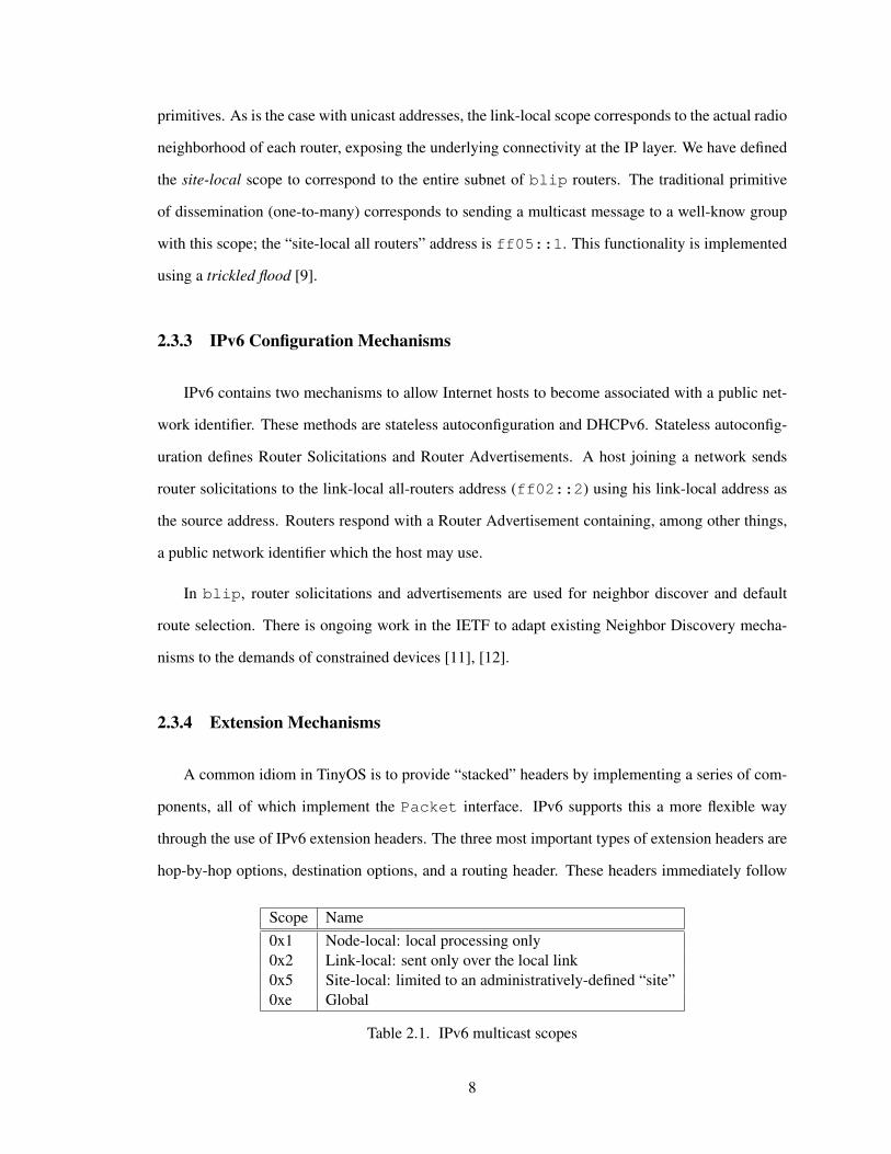
Scope Name0x1 Node-local: local processing only0x2 Link-local: sent only over the local link0x5 Site-local: limited to an administratively-defined “site”0xe Global
Table 2.1. IPv6 multicast scopes
8
the IPv6 header, and contain a common set of fields which allows routers to continue processing the
packet even if they do not recognize the header. Additionally, hop-by-hop and destination headers
allow multiple sub-options to be encapsulated within a single extension headers using the “Type-
Length-Value”, or TLV encoding.
We found that the ability to “piggyback” additional data into outgoing datagrams was an im-
portant enabler, because it allows protocols to reduce their overall message complexity or enables
them to include additional routing information. blip includes extensive support for inserting and
inspecting all three types of extension header, though the IPExtensions and TLVHeader inter-
faces. When a packet is being sent, it passes through the IPExtensions component. This component
is responsible for gather up any headers which are to be inserted, and so notifies any register ex-
tension header providers that the outgoing packet is about to be sent. These components can then
inspect the headers and payload, and return a pointer to a new extension header, if they wish; each
such header is prepended to the packet.
One concrete use case of this component is for the tracking of flows across the network; for
diagnostic use or performance analysis, it is convenient to be able to associate a particular packet in
flight with its origination, which could be several hops away. The TrackFlows component inserts
a sequence number as a hop-by-hop extension header on all outbound unicast flows. Routers along
the the path then print this sequence number to a serial console; using the log files from all network
nodes we can reconstruct a full trace of the packet.
There are several other important uses of these extension headers within blip, and we have
become convinced that using the IPv6 mechanisms for adding data is both principled and efficient
way of extending packet formats.
2.4 Transport Protocols
In IP networks, the transport protocol is responsible for managing the flow of data between
hosts on the network, and dispatching that data once it reaches its endpoint. Although it has been
suggested that neither TCP nor UDP is completely optimal for the common case of data collection,
9
these protocols are too prevalent to ignore. blip provides implementations of both protocols to
enable quick application development
2.4.1 UDP
The User Datagram Protocol consists of an 8-octet header, containing source and destination
port IDs, a checksum, and a length field. Application data payloads are otherwise sent using only
the bare IP datagram functionality, and thus subject to the underlying network reliability dynamics;
because of its low overhead and lack of buffering, it is a popular choice for constrained devices.
blip statically allocates sockets at compile time using nesc generics; applications needing a
socket allocate a new one using the UdpSocketC component. Each socket provides a simplified
version of the BSD sockets API, shown in Figure 2.3. If the application calls bind before issuing
any datagrams, the stack will bind the local endpoint of the socket connection to the specified port;
otherwise blip will choose an ephemeral port when the first packet is sent using sendto.
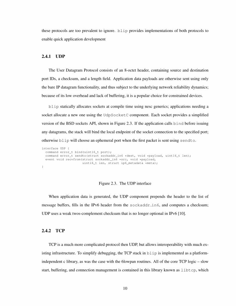
interface UDP {command error_t bind(uint16_t port);command error_t sendto(struct sockaddr_in6 *dest, void *payload, uint16_t len);event void recvfrom(struct sockaddr_in6 *src, void *payload,
uint16_t len, struct ip6_metadata *meta);}
Figure 2.3. The UDP interface
When application data is generated, the UDP component prepends the header to the list of
message buffers, fills in the IPv6 header from the sockaddr in6, and computes a checksum;
UDP uses a weak twos-complement checksum that is no longer optional in IPv6 [10].
2.4.2 TCP
TCP is a much more complicated protocol then UDP, but allows interoperability with much ex-
isting infrastructure. To simplify debugging, the TCP stack in blip is implemented as a platform-
independent c library, as was the case with the 6lowpan routines. All of the core TCP logic – slow
start, buffering, and connection management is contained in this library known as libtcp, which
10
can be quickly unit-tested on PC-class hardware; the bindings necessary to then cross-compile for
a TinyOS target are then very minimal.
blip makes several compromises in order to reduce the complexity of the TCP implementa-
tion. Firstly, no receive-side buffering is used; in-sequence TCP segments are delivered directly
to the application, while out of sequence segments are dropped, causing a full retransmission to
recover from. The interface is somewhat simplified – calling bind on a socket implies also calling
listen, and a call to accept never allocates a new socket, but rather replaces the socket that was
listening with one that is connected. This means that blip cannot listen for connections and then
accept multiple connections, as is typical for Internet servers. Although the underlying libtcp
would support this, allowing it in TinyOS would most likely require applications to dynamically
allocate memory, which is something to be avoided in the embedded setting.
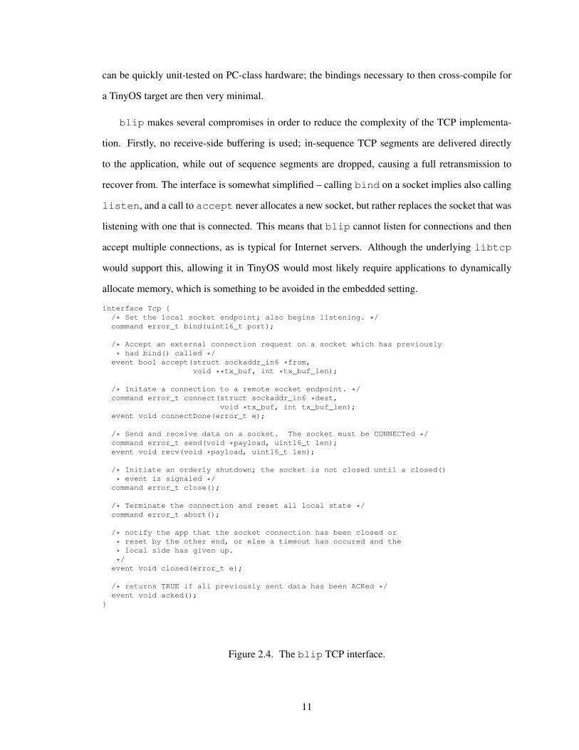
interface Tcp {/* Set the local socket endpoint; also begins listening. */command error_t bind(uint16_t port);
/* Accept an external connection request on a socket which has previously
* had bind() called */event bool accept(struct sockaddr_in6 *from,
void **tx_buf, int *tx_buf_len);
/* Initate a connection to a remote socket endpoint. */command error_t connect(struct sockaddr_in6 *dest,
void *tx_buf, int tx_buf_len);event void connectDone(error_t e);
/* Send and receive data on a socket. The socket must be CONNECTed */command error_t send(void *payload, uint16_t len);event void recv(void *payload, uint16_t len);
/* Initiate an orderly shutdown; the socket is not closed until a closed()
* event is signaled */command error_t close();
/* Terminate the connection and reset all local state */command error_t abort();
/* notify the app that the socket connection has been closed or
* reset by the other end, or else a timeout has occured and the
* local side has given up.
*/event void closed(error_t e);
/* returns TRUE if all previously sent data has been ACKed */event void acked();
}
Figure 2.4. The blip TCP interface.
11
Finally, the blip TCP stack requires applications to provide the buffer for outgoing data: this
is required whenever the application calls connect to initiate a new socket connection to a remote
endpoint, or the application uses the accept event to respond to an external connection request.
Each of these calls require the application to return a buffer to use for storing data until the other
end of the connection has acknowledged it. The buffer is managed by the TCP stack until the socket
is closed.
Choosing to have the application provide a buffer which is then managed by the TCP stack
diverges from what is the current de facto standard for embedded TCP stacks, uIP [13]. In that
model, the stack performs no buffering whatsoever, but requires the application to implement a
callback which, when called, will return the last segment sent but not acknowledged. Although this
approach can reduce memory consumption since most applications will be sending data which is
already stored in RAM, we felt that implementing buffering in the stack was an important interface
simplifications; applications sending data over TCP can use sendto to hand off the data to the
stack, even using multiple calls to push bytes into the byte stream, and then inquire at a later point
if all of of the data has been acknowledged.
2.5 Tools
To this point, we have considered the structure of blip providing the IPv6 networking ab-
straction. However, the full blip distribution includes many other application-layer tools to ease
application writing.
HTTP HTTP, a common application-layer protocol with wide uses sits on top of a TCP socket.
blip provides a simple HTTP implementation to allow application writers to implement
web services.
nwprog TinyOS includes support for storing program images in external flash and booting into
them, using the Deluge dissemination protocol and tosboot bootloader. blip reuses parts of
this software and uses a TFTP-like transport protocol for transmitting new images to motes
running blip.
12
Shell Interactive debugging on motes has not typically been practical, since there is not normally
a routing protocol which enables two-way communication. blip provides software support
for easily extending a text-based interface to mote functionality via the ShellCommandC
component. Using builtins, implementers can easily inspect the external flash or test network
connectivity using ping; they frequently extend the functionality to also allow interacting
with custom sampling drivers for a particular application.
Time For many applications we have encountered, the tight time synchronization provided by pro-
tocols like FTSP [14] is overkill; a resolution of a few seconds in sufficient. This closely
mirrors the situation in the Internet, where cryptographic protocols such as SSL require time
synchronization within minutes, mostly to prevent replay attacks. Using the multicast func-
tionality, blip can provide Unix timestamps with very low overhead and an accuracy of a
few seconds.
13
Chapter 3
The Hydro Routing Protocol
3.1 Overview
Data collection represents a significant fraction of network traffic in many monitoring applica-
tions, as has been well-documented in the literature [15]–[17]. In these systems, in-network nodes
gather sensor data locally and either trickle their readings frequently or send bulk data sets periodi-
cally to a remote server with the border routers acting as data sinks. Since most applications employ
some form of collection, it is critical to optimize collection as a basic network primitive. However,
point-to-point traffic also occurs, especially since these networks are now embracing IP. Collection
and dissemination alone are insufficient, since they lead to inefficient application modalities such as
flooding the entire network to deliver a command to a single node.
In many cases, point-to-point routing would be used to initiate data transfer, send end-to-end
acknowledgements like in TCP and Flush, or for carrying out infrequent network diagnostics with
ping and traceroute. In some cases, traffic flows exist between a “root” node and some other
node in a network. In other cases, point-to-point flows exist between arbitrary nodes in the network,
like a control path between a light switch and light bulb. A successful point-to-point routing protocol
will make few demands on nodes in the first case and will make demands proportional to some
measure of the workload (e.g. number of flows, nodes, or neighbors) in the second case.
The key insight underlying this work is that while point-to-point routing is becoming more
14
important, the space, time, and message overhead of point-to-point routing must be proportional to
its often minor yet critical usage in practice. In other words, application developers are willing to
pay for point-to-point routing only if its cost is negligible when it goes unused and is proportional
to the degree of point-to-point traffic when it does get used. Unfortunately, existing point-to-point
routing protocols like S4, BVR, and DYMO do not satisfy this load-proportionality. This fact may
be one reason they are relatively unused in practice, especially since a collection protocol may still
be necessary and run in parallel.
In order to meet the requirements of robust collection, point-to-point communication, and low
footprint, we present Hydro, a hybrid routing protocol for L2Ns that provides both centralized con-
trol and local agility. Hydro uses a distributed algorithm to form a DAG for routing data from
in-network nodes to border routers, allowing nodes to maintain multiple options that are ranked
through data-driven link estimation. Nodes piggyback topology reports on periodic collection traf-
fic, allowing border routers to build and maintain a global view of the topology. The DAG provides
basic triangle point-to-point routing by allowing nodes to forward packets to a border router, which
subsequently source routes them to the appropriate destination. Hydro builds on prior work by
adding a centralized optimization in which border routers insert routing table entries at the appro-
priate nodes, reducing the transmission stretch between communicating endpoints without the need
for excessive state or complexity at the nodes.
We begin by taking a critical look at existing wireless and internet routing and control proto-
cols. From internet work, we distill a set of lessons dealing with key requirements for centralized
platforms. Using literature from the wireless space, we synthesize a set of building blocks to help
us meet these requirements. Our detailed design lays out our the mechanisms and policies making
up Hydro. Our key contribution is showing that providing simple, efficient point-to-point routing in
low-power networks is possible by taking advantage of the lessons of collection routing protocols,
as well as additionally placing a small number of routing “hints” into the network. We evaluate Hy-
dro on two testbeds and one application deployment, and note that the protocol has been deployed
in three different production-level networks for over six months, operating over a low-power MAC
when necessary.
15

3.2 Background
In this section, we examine existing solutions in the space, highlighting elements which serve as
building blocks for our design and their shortcomings. Creating a distinct control plane for routing
is not a novel idea, and so we examine related works in internetworking. Such work served as
inspiration for our design, yet we also discuss barriers that prevent such works from being naturally
portable to L2Ns.
3.2.1 Existing Low-Power Protocols
Routing has been an integral part of L2Ns since their emergence, as data and commands had to
be relayed between nodes. Initially, as many of the deployments focused on various types of moni-
toring, the predominant communication paradigm was Collection-Oriented, or many-to-one routing.
By association Dissemination-Oriented, or one-to-many, routing also emerged because of the need
to send commands to the nodes (e.g. for time synchronization). We examine the progression and
state-of-the art for these constrained L2N routing protocols.
In addition, as the set of potential application domains expanded, the need for richer and
fuller routing protocols became clear, i.e. those that support unicast and multicast communication
paradigms; we examine these in this section as well.
Collection-Oriented Protocols
Most collection protocols are tree-based. MintRoute [18] was one of the initial routing proto-
cols for L2Ns. Starting with the gateway, or base station node, beacon messages announce the cost
to reach the gateway in terms of hops, as well as ETX, or expected transmissions. While MintRoute
was successful, it’s main shortcomings stemmed from the limited sophistication of its link estima-
tion and loss response techniques, which reduced efficiency in difficult RF environments.
The successor to MintRoute was CTP [8]. CTP developed a more accurate link estimator, in
which control and data traffic were used to inform link estimates, although two different link esti-
mators were kept. Multiple potential next-hop parents are maintained, although only one was used
16
at any given time. In one test, CTP displayed 97% overall reliability in a difficult RF environment,
as opposed to the 70% reliability obtained by MintRoute.
CentRoute [19] provides centralized tree routing, allowing for dissemination of tasklets and
collection of information in the Tenet [20] architecture. A single node serves as the sink, and other
nodes in the network send join request messages which are forwarded to the sink. Once created,
the tree is frozen unless some threshold of failures occur, after which a node disengages and begins
the join process anew. This approach is limited to single destination routing, and also affords no
flexibility for dynamic topology conditions unless links completely break.
Koala [21] is designed to provide mechanisms to enable efficient data retrieval from in-network
nodes. It presents centralized mechanisms similar to those used by Hydro, in which nodes explore
their neighborhood, and provide this information to a central controller, which subsequently installs
an appropriate route in the network. However, similar to CentRoute, these mechanisms are only
targeted towards collecting data to a root. Further, it does not position these mechanisms within
a broader architecture or investigate their performance under different conditions; the focus of the
work is a MAC-layer technique called Low Power Probing.
TSMP [22], incorporated into the WirelessHART standard, is a well-established industry ap-
proach that includes centralize scheduling of channel resources to achieve predictable latencies.
However, although little technical data is available, it operates at the link-layer, using channel hop-
ping, and does not provide any routing capabilities specified in publicly available documentation. Its
tight scheduling of media accesses differs significantly from the functionality of our border routers,
which contain only soft state and are relatively asynchronous.
Hui presented a complete IPv6 network architecture for L2Ns, which includes a low power link
along with network and transport layers adapted to the unique characteristics of these networks [2].
This work adapted collection to the IP architecture by conceptualizing it as choosing an IP default
route. It also provided unicast capabilities by allowing a controller to efficiently communicate with
individual nodes by source routing the packet, forming the basis for triangle routing of intra-network
traffic. However, such an approach also incurs unnecessarily high stretch, and naturally forms
bottleneck links around the controller. This basic design represents the leading edge of collection
17
research, and formed Hydro’s basic template; we extend it with optimizations for point-to-point
traffic.
Other Routing Protocols
BVR [23] was a geographical location-based routing protocol for L2Ns. A set of landmark
beacons are selected whose identity is known by all nodes in the network. Every node is given
a virtual coordinate, which is the vector of distances to all beacons in the network. When a node
wants to send a packet to a destination node, it greedily forwards the packet along routes that move it
closer to the destination. BVR suffers from poor transmission and routing stretch, particularly as the
network grows in size [24]. Another difficulty is that in such a network, the identity of the beacons
must be known a priori, and can not be modified dynamically without a location service [25].
S4 [24], is designed to provide small stretch and state in order to enable scalable routing. It
utilizes a modified compact routing algorithm tailored for L2Ns. S4 has a theoretical worst case
routing stretch of 3, although published results indicate an average routing stretch of 1.2 while
maintaining O(√
N) state. Like BVR, deploying S4 would require also designing a distributed
directory service. Neither of these protocols optimize for the common workload where most traffic
is destined towards an egress point; unlike S4 and BVR’s homogeneous network, Hydro starts with
optimizing collection and emphasizing heterogeneity.
3.2.2 Ad-Hoc Networking Protocols
Finally, is also an extensive literature on fully distributed routing protocols for ad-hoc wireless
networks. AODV [26] uses flooded RREQ messages to discover paths to destinations on demand,
with intermediate nodes creating hop-by-hop entries for bidirectional flows. DSR [27] is also an
on-demand routing protocol, but uses source routing to route packets. OLSR [28] is a link state
algorithm that uses multipoint relays to reduce the flood of link-state advertisements. 802.11s, a
draft mesh routing standard uses a variant of AODV called AODV-RM for intra-subnet point-to-
point communication, but optimizes for an access network’s workload by proactively building a
routing tree towards egress points [29].
18
These and other protocols provide point-to-point routing capabilities in wireless networks. Both
on-demand and link-state based solutions exist, but the focus is on providing reliable any-to-any
delivery in networks with mobile nodes that are resource rich. Consequently, most of these protocols
have large control traffic and/or state requirements. A protocol survey [5] recently evaluated the
specifications of the most widely used ad-hoc protocols against five criteria, and noted that in their
current form no ad-hoc protocol meets more than three of the five criteria.
3.2.3 Internet Solutions
The concept of centralized routing, or separating the control and data planes, is not a novel
one; we explore several existing protocols later in this section that embrace a centralized paradigm.
However, these solutions were designed primarily for the Internet, characterized by low churn and
high bandwidth. This is in stark contrast to the high-churn, low-bandwidth nature of typical L2N
environments.
The most conceptually similar work is Ethane [30], a centralized architecture for implementing
high-level security policies. Designed for large enterprise networks, the network is divided into four
tiers: controllers, switches, end hosts or servers, and users. Network administrators specify high-
level access policies, such as restricting which servers a certain user may communicate with. Each
switch maintains a flow table against which it can classify incoming packets using a packet header’s
10-tuple. If no applicable entry exists, the packet is forwarded to the controller. The controller
consults its policy specification, and installs flow entries along the path. Whenever a switch is
connected to the network, it registers with the controller, and establishes a secure channel to it.
When a server or middlebox joins the network, it also registers with the controller, reporting the
connecting switch and port. Consequently, the controller maintains a complete and accurate view
of the topology. Each switch maintains a flow table in which it can match packet 5-tuples. If no
applicable entry exists, the packet is forwarded to the controller. The controller consults its policy
specification, and installs hop-by-hop flow entries along the path.
Key elements visible in this design include forming a channel and “default routing” to a con-
19
troller, and maintaining global topology. Hydro also addresses these issues, but the details differ
significantly when no wired infrastructure is available.
A number of other centralized internet routing designs exist, which we mention briefly for
completeness. Feamster’s Routing Control Platform, implemented by Caesar, made the case for
separating the control aspect of routing from routers [31], [32]. Greenberg et al. present 4D [33],
[34], a general framework for separating routing from routers. The framework consists of four
components: a decision plane, a dissemination plane, a discovery plane, and a data plane.
3.2.4 Towards a Hybrid Solution
From this disparate related work, we distill a few common components of successful centralized
control.
Reliable Path to Centralized controller A logical controller serves as the brain of the network,
gathering information from all the routers in the network, and disseminating control com-
mands. One of the key implications of this role hierarchy is the need for a stable channel
between the controller and all routers in the network at all times. In large wired networks,
creation of this channel is simplified by underlying data link layers: in Ethernets, the underly-
ing layer-2 spanning tree algorithm provides reachability between all switches and end-hosts
in a subnet.In contrast, no such natural mechanisms exist in L2N environments, and so the
network layer must build a robust path to the controller. We notice that much collection
research may be re-cast as attempting to provide just this functionality.
Consistent Global View of Topology One benefit of centralized routing is the ability to make rout-
ing decisions at a central location that has complete information about the state of the entire
network. Three main factors complicate this task in L2Ns: control traffic restrictions, mem-
ory constraints, and dynamic topology. Only a trickle of bandwidth is generally available to
propagate network state towards a control element. Links exhibit temporal and spatial vari-
ability, which complicates maintaining a consistent view of network links. Finally, memory
constraints prevent individual nodes from maintaining state for all nodes in the network, or
20
even the single-hop broadcast neighborhood. Therefore, forming the complete topology may
not be possible; we investigate the extent to which this is necessary.
Providing Reliability Over Lossy Links The target environment for the majority of existing rout-
ing protocols is often highly-reliable, in the form of either wired links, or single-hop wireless
links that provide relatively high reliability, through both link-layer and typically transport
layer retransmissions. In L2Ns, the low-power nature of the ratio leads to a small Signal-
to-Interference-and-Noise Ratio (SINR) on many links. As demonstrated by Srinivasan et
al. [35], the SINR of these links is often on the cusp of the necessary threshold to receive
a packet, which results in bimodal links due to variations in signal strength and interference
levels. Consequently, accurate link estimation and local repair techniques are critical.
Although it is not obvious that any element of centralized control is a natural fit for L2N rout-
ing since existing centralized solutions rely on assumptions which do not automatically hold in
this setting, research in the sensor network literature can be re-cast to help achieve the necessary
prerequisites.
3.3 Hydro Design and Operation
Hydro’s design is a marriage of centralized and distributed mechanisms: low-power nodes form
and maintain a distributed DAG that provides them with a set of default routes for communicating
with border routers. These border routers maintain a global view of the network using topology
reports received from each of the nodes, and subsequently install optimized point-to-point routes
within the network. These three mechanisms of distributed DAG formation, global topology forma-
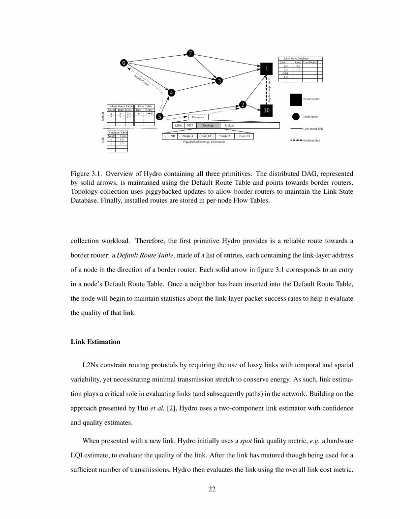
tion, and route install form the primitives for Hydro’s operation, and are shown in figure 3.1.
3.3.1 Distributed DAG formation
Most communication in L2Ns is data generated by network nodes being routed to data sinks.
In Hydro, border routers provide egress connectivity beyond the L2N to these data sinks and other
internet hosts. The distributed DAG provides a locally-maintained mechanism for optimizing the
21
L NH Neigh: 2 Cost: 2.5Neigh: 4 Cost: 1.6
Datagram
1
2
3
4
5
6
Default Route TableNeigh Hops Cost
4 2 2.42 1 1.2
Flow TableDest Route
LINK NET PayloadTopology
7
Neighbor TableNeigh Cost
4 1.62 2.5
Rou
ting
Lin
k
Link State DatabaseLink Cost Last Heard ...
5-25-4
4-32-10
...
2.51.5
Border router
Node router
Low-power link
10
Backhaul link
Rep
lica
tion
pro
toco
l
Piggybacked topology information
6 4 6
Installed route
Figure 3.1. Overview of Hydro containing all three primitives. The distributed DAG, representedby solid arrows, is maintained using the Default Route Table and points towards border routers.Topology collection uses piggybacked updates to allow border routers to maintain the Link StateDatabase. Finally, installed routes are stored in per-node Flow Tables.
collection workload. Therefore, the first primitive Hydro provides is a reliable route towards a
border router: a Default Route Table, made of a list of entries, each containing the link-layer address
of a node in the direction of a border router. Each solid arrow in figure 3.1 corresponds to an entry
in a node’s Default Route Table. Once a neighbor has been inserted into the Default Route Table,
the node will begin to maintain statistics about the link-layer packet success rates to help it evaluate
the quality of that link.
Link Estimation
L2Ns constrain routing protocols by requiring the use of lossy links with temporal and spatial
variability, yet necessitating minimal transmission stretch to conserve energy. As such, link estima-
tion plays a critical role in evaluating links (and subsequently paths) in the network. Building on the
approach presented by Hui et al. [2], Hydro uses a two-component link estimator with confidence
and quality estimates.
When presented with a new link, Hydro initially uses a spot link quality metric, e.g. a hardware
LQI estimate, to evaluate the quality of the link. After the link has matured though being used for a
sufficient number of transmissions, Hydro then evaluates the link using the overall link cost metric.
22
We use link-layer acknowledgement frames on all unicast link traffic, and maintain a link quality
estimate based on the ack reception rate: as a result, our link estimator strongly prefers bidirectional
links. To account for the temporal variability of links, Hydro maintains both long-term and short
term link estimates. Both estimators use the same metric (ETX) but with different time horizons so
as to manage the agility/stability tradeoff.
Router Discovery
Hydro uses Router Advertisement and Router Solicitation messages to achieve router discovery,
co-opting existing IPv6 Neighbor Discovery [11] mechanisms. Router solicitation messages are sent
using binary exponential timers, and this timer is reset when either a node boots, or when no default
route (which we discuss in Section 3.3.1) to a border router exists. Nodes that receive a router
solicitation message respond with a router advertisement if they have a valid default route.
A router advertisement consists of two parts: (1) an Overall Route Cost, which we define as
the path cost of the advertising node’s default route, and (2) a willingness value, which indicates
the degree to which the advertising node is willing to forward traffic for other nodes. Such a metric
accounts for a heterogeneous network, in which battery-powered and mobile nodes would rather
shift forwarding responsibilities to mains-powered or stationary nodes.
Default Route Formation
Existing collection-based protocols demonstrated that providing multiple routes to a given desti-
nation significantly improves reliability in L2Ns [2], [8]. Hydro’s Default Route Table is an ordered
list of next hop addresses for communicating with border routers. Each default route entry contains
the address of the next-hop in the path, the route cost advertised by the next-hop, the link cost esti-
mate for communicating with the next-hop (and the corresponding confidence), and the advertised
willingness. The Default Route Table is sorted based on the Overall Route Cost (the sum of the
advertised route cost and the link cost estimate), the Confidence, and the Willingness value. The
top entry in the table is referred to as the Primary Default Route, and the Overall Route Cost of this
23
particular entry is used for Router Advertisements. A significant change in the overall route cost of
the primary default route triggers additional Router Advertisements to maintain consistency.
Resource constraints prevent the Default Route Table from growing in size with the one-hop
neighborhood of a node, and as such a comparison in and eviction mechanism is needed. If the
Default Route Table is full, the same sorting mechanisms are used to determine whether to evict the
bottom entry in favor of a newly received router advertisement. The one caveat is that entries where
the next-hop link has not yet achieved maturity can not be evicted. While this potentially delays
the convergence of the Default Route Table, it does prevent volatile thrashing and allows for more
accurate evaluation of routes.
3.3.2 Global Topology Construction
The second primitive Hydro requires is the collection of topology information from the network:
in order to execute its duties as a central point of control, a border router must build a global view
of the topology. However, this task is complicated by multiple factors: restrictions on control traffic
make it impractical for the nodes to send their complete link-state to the border router; furthermore,
memory constraints prevent nodes from even maintaining a list of all neighbors, making creation of
the complete global topology impossible.
In Hydro, each node in the network creates Topology Reports to be sent to a border router.
Topology reports contain only the top few “mature” entries in the Default Route Table. In addition,
Hydro allows nodes to optionally insert Node Attributes in topology reports. These Node Attributes
are application specific, and can be static (e.g. installed memory or power source), or dynamic (e.g.
energy left or queue length), to enable more complex routing policies.
Topology reports are sent to a border router periodically using a default route; they are op-
portunistically piggybacked on data traffic whenever an application generates sufficiently frequent
traffic. The unpacked datagram in figure 3.1 shows how topology information is added to data traffic
using an optional extension header; using this mechanism, the overhead is only incurred on packets
actually containing topology updates.
The border router aggregates these topology reports to create a global view of the topology,
24

known as the Link State Database. Figure 3.1 shows a partial view of the LSDB maintained by
controller 1: for instance, the link from 5 to 2, being reported in the exploded packet is present in
the database with cost 2.5. While this view does not include all links in the physical network, it is a
subset of high-quality, bidirectional links with accurate link cost estimates.
3.3.3 Centralized Route Installation
The combination of distributed DAG formation and a global topology database enables point-to-
point communication through triangle routing. The final Hydro primitive allows state to be installed
in the network to optimize active flows. A border router uses Route Installs to update a node’s Flow
Table. When a node receives a Route Install, it inserts or updates an entry in the Flow Table. Each
Route Install has two parts:
• Flow Match: The criteria used to determine whether a given packet matches a flow table
entry. By default Hydro uses the packet destination, but more complex flow matches based
on additional fields such as the packet source, traffic type, or flow label are possible.
• Flow Path: The actual route that matching packets use. Hydro stores the complete path to
the destination used in a source routing header; section 3.6.2 discusses an extension to enable
hop-by-hop route installs.
The policy for when routes should be installed may either be a default policy, or optimized for
specific workloads. By default, Hydro installs routes the first time they are used. If the border router
receives a packet that originated in the subnet and is destined for another node in the same subnet,
it calculates the optimal path between the source-destination pair. If this optimal path includes
a border router, then it simply forwards the packet as described in section 3.3.4. Otherwise, the
border router sends a Route Install message to the source of the packet, in addition to forwarding
the packet to the destination. Figure 3.1 shows the result of one of these Route Install messages
in the Flow Table for node 5: the table contains an entry indicating that a route to node 6 with
intermediate hop 4. This route will be used to insert a source routing header into packets destined
to node 6.
25
Certain optimizations are possible as well through the use of special installation policies.
Transport-layer acknowledgements such as TCP ACKs often create bidirectional flows, and so Hy-
dro allows the border router to specify a bidirectional Route Install. In this case, the route install
message received by the source is forwarded to the destination, which simply reverses the included
path. As a further optimization for reversible route installs, the border router simply piggybacks
the route install on the packet that is being forwarded to the destination, which then piggybacks the
route install on its next message to the original packet source. Using this mechanism, routes can be
installed with explicit control traffic.
Hydro does not maintain information about which routes are installed at which nodes in the
network, and route installs are never explicitly expired in the network. Rather, an installed route
is used until a link failure, at which time the packet is rerouted along a default route to the border
router; the border router may then install a fresh route. This ensures that routes are only installed
(and maintained) on demand. We discuss state management in Hydro in more detail in section 3.3.6.
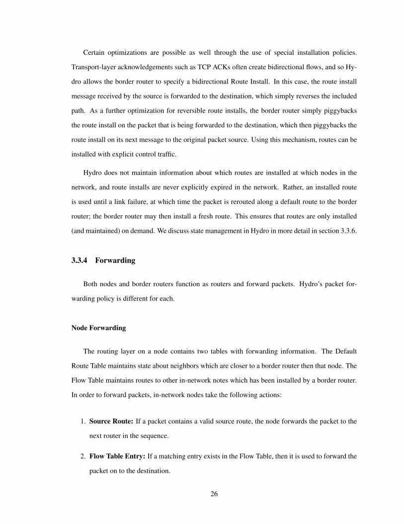
3.3.4 Forwarding
Both nodes and border routers function as routers and forward packets. Hydro’s packet for-
warding policy is different for each.
Node Forwarding
The routing layer on a node contains two tables with forwarding information. The Default
Route Table maintains state about neighbors which are closer to a border router then that node. The
Flow Table maintains routes to other in-network notes which has been installed by a border router.
In order to forward packets, in-network nodes take the following actions:
1. Source Route: If a packet contains a valid source route, the node forwards the packet to the
next router in the sequence.
2. Flow Table Entry: If a matching entry exists in the Flow Table, then it is used to forward the
packet on to the destination.
26
3. Default Route: If neither a source route nor flow entry is available, packets are forwarded
along a default route to a border router.
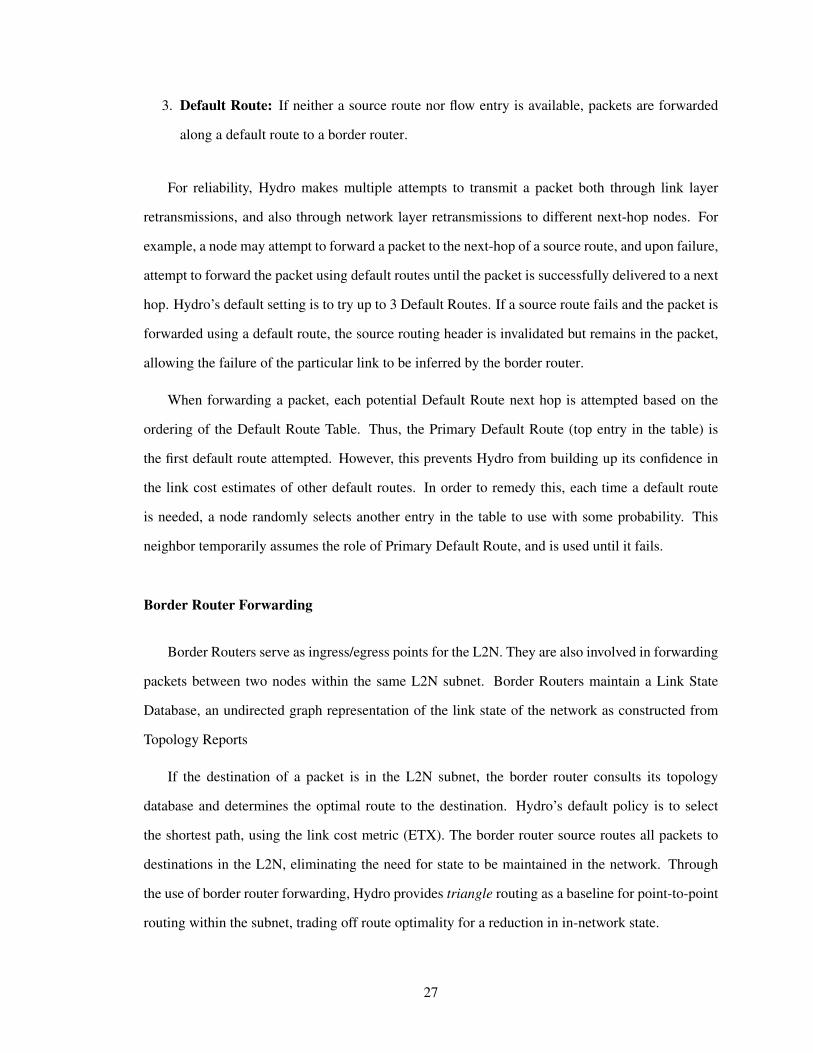
For reliability, Hydro makes multiple attempts to transmit a packet both through link layer
retransmissions, and also through network layer retransmissions to different next-hop nodes. For
example, a node may attempt to forward a packet to the next-hop of a source route, and upon failure,
attempt to forward the packet using default routes until the packet is successfully delivered to a next
hop. Hydro’s default setting is to try up to 3 Default Routes. If a source route fails and the packet is
forwarded using a default route, the source routing header is invalidated but remains in the packet,
allowing the failure of the particular link to be inferred by the border router.
When forwarding a packet, each potential Default Route next hop is attempted based on the
ordering of the Default Route Table. Thus, the Primary Default Route (top entry in the table) is
the first default route attempted. However, this prevents Hydro from building up its confidence in
the link cost estimates of other default routes. In order to remedy this, each time a default route
is needed, a node randomly selects another entry in the table to use with some probability. This
neighbor temporarily assumes the role of Primary Default Route, and is used until it fails.
Border Router Forwarding
Border Routers serve as ingress/egress points for the L2N. They are also involved in forwarding
packets between two nodes within the same L2N subnet. Border Routers maintain a Link State
Database, an undirected graph representation of the link state of the network as constructed from
Topology Reports
If the destination of a packet is in the L2N subnet, the border router consults its topology
database and determines the optimal route to the destination. Hydro’s default policy is to select
the shortest path, using the link cost metric (ETX). The border router source routes all packets to
destinations in the L2N, eliminating the need for state to be maintained in the network. Through
the use of border router forwarding, Hydro provides triangle routing as a baseline for point-to-point
routing within the subnet, trading off route optimality for a reduction in in-network state.
27
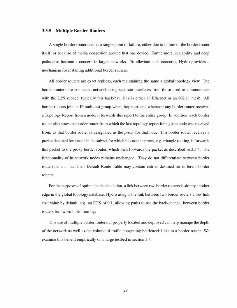
3.3.5 Multiple Border Routers
A single border router creates a single point of failure, either due to failure of the border router
itself, or because of media congestion around that one device. Furthermore, scalability and deep
paths also become a concern in larger networks. To alleviate such concerns, Hydro provides a
mechanism for installing additional border routers.
All border routers are exact replicas, each maintaining the same a global topology view. The
border routers are connected network using separate interfaces from those used to communicate
with the L2N subnet: typically this back-haul link is either an Ethernet or an 802.11 mesh. All
border routers join an IP multicast group when they start, and whenever any border router receives
a Topology Report from a node, it forwards this report to the entire group. In addition, each border
router also notes the border router from which the last topology report for a given node was received
from, as that border router is designated as the proxy for that node. If a border router receives a
packet destined for a node in the subnet for which it is not the proxy, e.g. triangle routing, it forwards
this packet to the proxy border router, which then forwards the packet as described in 3.3.4. The
functionality of in-network nodes remains unchanged. They do not differentiate between border
routers, and in fact their Default Route Table may contain entries destined for different border
routers.
For the purposes of optimal path calculation, a link between two border routers is simply another
edge in the global topology database. Hydro assigns the link between two border routers a low link
cost value by default, e.g. an ETX of 0.1, allowing paths to use the back-channel between border
routers for “wormhole” routing.
This use of multiple border routers, if properly located and deployed can help manage the depth
of the network as well as the volume of traffic congesting bottleneck links to a border router. We
examine this benefit empirically on a large testbed in section 3.4.
28
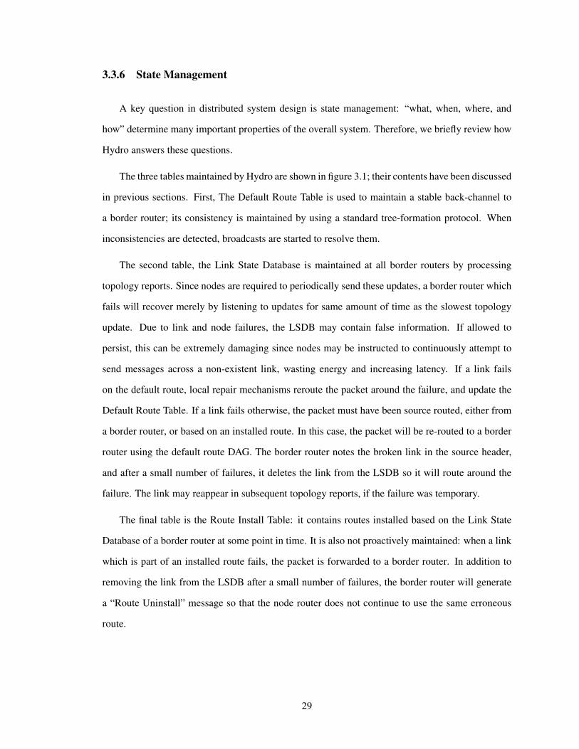
3.3.6 State Management
A key question in distributed system design is state management: “what, when, where, and
how” determine many important properties of the overall system. Therefore, we briefly review how
Hydro answers these questions.
The three tables maintained by Hydro are shown in figure 3.1; their contents have been discussed
in previous sections. First, The Default Route Table is used to maintain a stable back-channel to
a border router; its consistency is maintained by using a standard tree-formation protocol. When
inconsistencies are detected, broadcasts are started to resolve them.
The second table, the Link State Database is maintained at all border routers by processing
topology reports. Since nodes are required to periodically send these updates, a border router which
fails will recover merely by listening to updates for same amount of time as the slowest topology
update. Due to link and node failures, the LSDB may contain false information. If allowed to
persist, this can be extremely damaging since nodes may be instructed to continuously attempt to
send messages across a non-existent link, wasting energy and increasing latency. If a link fails
on the default route, local repair mechanisms reroute the packet around the failure, and update the
Default Route Table. If a link fails otherwise, the packet must have been source routed, either from
a border router, or based on an installed route. In this case, the packet will be re-routed to a border
router using the default route DAG. The border router notes the broken link in the source header,
and after a small number of failures, it deletes the link from the LSDB so it will route around the
failure. The link may reappear in subsequent topology reports, if the failure was temporary.
The final table is the Route Install Table: it contains routes installed based on the Link State
Database of a border router at some point in time. It is also not proactively maintained: when a link
which is part of an installed route fails, the packet is forwarded to a border router. In addition to
removing the link from the LSDB after a small number of failures, the border router will generate
a “Route Uninstall” message so that the node router does not continue to use the same erroneous
route.
29
3.4 Evaluation
This section evaluates the performance of Hydro on several key metrics across multiple net-
works. In one application, we evaluate the performance of 57 nodes running Hydro for over six
months in a real deployment. On two experimental testbeds, we evaluate Hydro’s scalability, per-
formance, and resilience across a range of workloads and failure conditions.
3.4.1 Metrics
Centralized routing over low-power and lossy wireless networks raises many concerns that must
be addressed in a successful design. These concerns, and Hydro’s response to them, include the
following:
Reliability. The lossy nature of wireless mesh networks means that implementing reliability at
end hosts alone is insufficient and that support for both hop-by-hop retransmissions and end-to-end
route adaptations are needed.
Convergence. Centralized routing protocols must gather topology data at one (or more) “cen-
tral” locations before routing can take place, and so link dynamics, coupled with constraints on
control traffic, can make converging on a consistent view of the network a challenge.
Stretch. Near optimal routes, with respect to metrics like transmission stretch, are key to con-
serving energy and lowering congestion in L2Ns.
Agility/Stability. Centralized routing protocols incur delay when responding to local transients
like link and node churn.
Scalability. Centralizing the points of control can make scaling a network difficult, and routing
in large networks with limited state and constrained control traffic further exacerbate this scaling
challenge.
30
3.4.2 Methodology
We use two testbeds and a real deployment to evaluate Hydro. Testbed A is a ceiling-mounted
network of 48 nodes across a single floor and a network diameter of 3-5 hops, depending on envi-
ronmental factors. Testbed B consists of a network of 125 nodes spread across three floors, with a
diameter of 7-9 hops. Both testbeds are equipped with wired backchannels, which we use to collect
packet traces that allow us to track the progress of packets through the network. The real deploy-
ment consists of 49 nodes spread across four floors of an office building, with the nodes placed in
various locations, such as under desks, inside a refrigerator, or on the ceiling. An additional eight
nodes are installed in a remote residential environment, resulting in a total deployment size of 57
nodes.
For the baseline workload in these experiments, all nodes report data to a border router every 30
seconds (with no other form of traffic). We define a flow to be traffic between a source / destination
pair, and in our experiments, we use ICMP ping messages, separated by 2 seconds for multi-packet
flows. In addition, all experiments are given time to bootstrap the network topology formation,
except as noted.
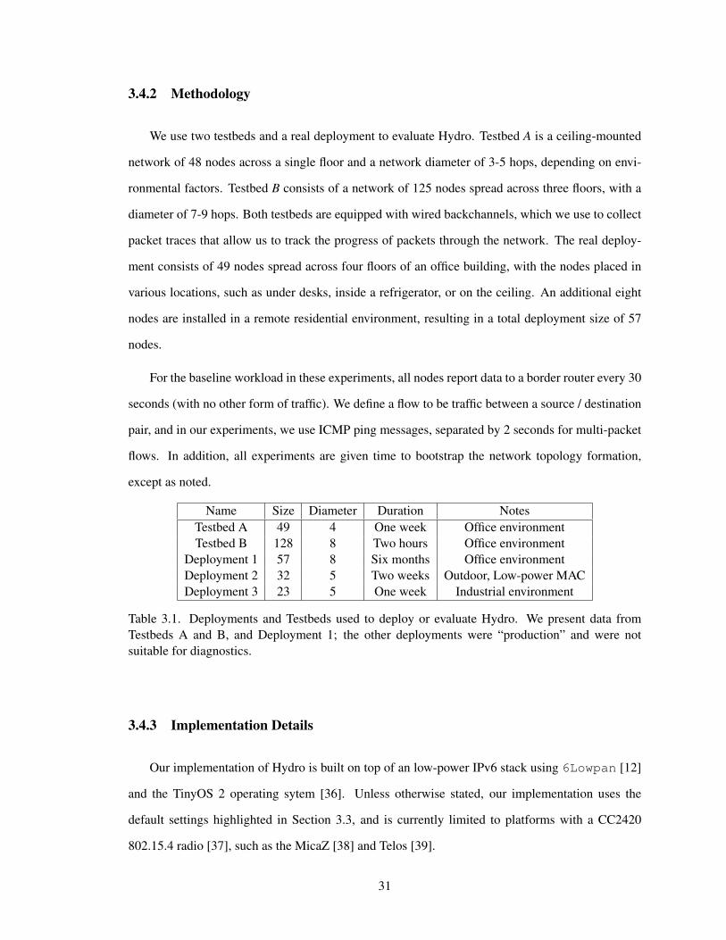
Name Size Diameter Duration NotesTestbed A 49 4 One week Office environmentTestbed B 128 8 Two hours Office environment
Deployment 1 57 8 Six months Office environmentDeployment 2 32 5 Two weeks Outdoor, Low-power MACDeployment 3 23 5 One week Industrial environment
Table 3.1. Deployments and Testbeds used to deploy or evaluate Hydro. We present data fromTestbeds A and B, and Deployment 1; the other deployments were “production” and were notsuitable for diagnostics.
3.4.3 Implementation Details
Our implementation of Hydro is built on top of an low-power IPv6 stack using 6Lowpan [12]
and the TinyOS 2 operating sytem [36]. Unless otherwise stated, our implementation uses the
default settings highlighted in Section 3.3, and is currently limited to platforms with a CC2420
802.15.4 radio [37], such as the MicaZ [38] and Telos [39].
31
Border Routers exist in two forms: either a normal PC with a connected node for interfacing
with the L2N, or an embedded Linux device with an integrated 802.15.4 radio.
One limitation of our implementation independent of Hydro’s design is the fact that packets are
acknowledged at the link layer, although they may be dropped at the network layer due to a full
forwarding queue. In such cases, the source assumes the packet was succesfully received (and will
be forwarded), and so no retransmission is attempted and the packet delivery ratio suffers.
3.4.4 Distributed DAG Formation
The distributed DAG is critical to Hydro’s functionality. It serves as the dynamic control plane
for delivering topology reports to the border router, and also serves as the last resort for delivering
unicast traffic when an installed route has failed or none exists. As such, it is imperative that this
underlying DAG provide a reliable channel for traffic from the nodes to the border router.
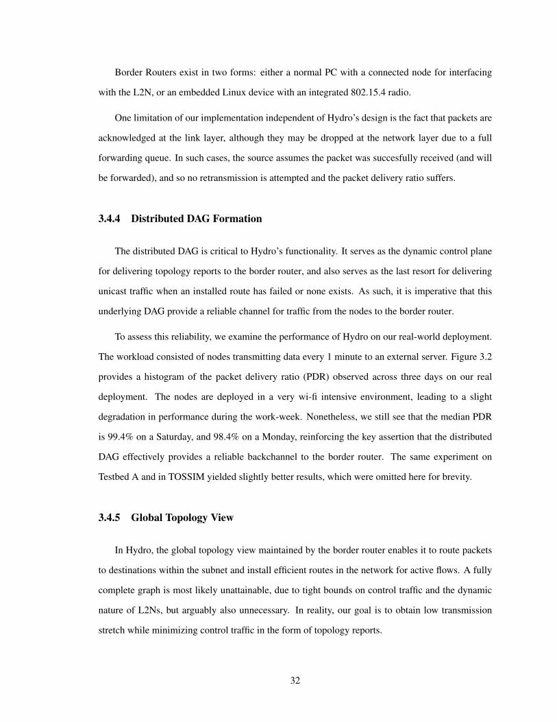
To assess this reliability, we examine the performance of Hydro on our real-world deployment.
The workload consisted of nodes transmitting data every 1 minute to an external server. Figure 3.2
provides a histogram of the packet delivery ratio (PDR) observed across three days on our real
deployment. The nodes are deployed in a very wi-fi intensive environment, leading to a slight
degradation in performance during the work-week. Nonetheless, we still see that the median PDR
is 99.4% on a Saturday, and 98.4% on a Monday, reinforcing the key assertion that the distributed
DAG effectively provides a reliable backchannel to the border router. The same experiment on
Testbed A and in TOSSIM yielded slightly better results, which were omitted here for brevity.
3.4.5 Global Topology View
In Hydro, the global topology view maintained by the border router enables it to route packets
to destinations within the subnet and install efficient routes in the network for active flows. A fully
complete graph is most likely unattainable, due to tight bounds on control traffic and the dynamic
nature of L2Ns, but arguably also unnecessary. In reality, our goal is to obtain low transmission
stretch while minimizing control traffic in the form of topology reports.
32
< .90 0.92 0.94 0.96 0.98 1.000
5
10
15
20
25
30
Fraction of Data
Nu
mb
er o
f N
od
es
Data Yield
SaturdaySundayMonday
Figure 3.2. CDF of collection packet delivery ratio observed over three days in a real-world deploy-ment.
0 20 40 60 80 100 120 140 160 180 200
0
0.5
1
1.5
2
2.5
3
3.5
4
4.5
5
Time (minutes)
Ave
rage
rep
orte
d ro
uter
deg
ree
5 minute report interval30 second report interval30 second report, P(explore) = .125
(a) Average node degree
0 1 2 3 4 5 6 7
0
0.1
0.2
0.3
0.4
0.5
0.6
0.7
0.8
0.9
1
Average pairwise transmission stretch
Fra
ctio
n of
pop
ulat
ion
4 minutes9 minutes100 minutes8.5 hours
(b) Stretch (30-second interval)
0 1 2 3 4 5 6 7
0
0.1
0.2
0.3
0.4
0.5
0.6
0.7
0.8
0.9
1
Average pairwise transmission stretch
Fra
ctio
n of
pop
ulat
ion
4 minutes9 minutes100 minutes8.5 hours
(c) Stretch (5-min interval)
Figure 3.3. Average degree of a node in the border router’s global topology view as a function oftime, topology report rate, and rate of exploration, and the corresponding stretch.
We begin by examining the average degree of nodes in the global topology view at the border
router. The intuition is that a larger average degree indicates that an increasing portion of the real
topology has been captured, and so that links which reduce stretch are more likely to have been
discovered. Two factors determine node degree: the Topology Report Interval, which dictates how
often nodes propagate information to the border router, and the exploration rate, which determines
how aggressive nodes are in gathering information about neighboring nodes 1. In essence, the degree
of a node in the global topology is determined by the number of neighbors in the node’s topology
report, as well as the number of other node’s topology reports that this particular node appears in.1In our implementation, a maximum of 4 mature neighbors are be reported in a topology report. Any new information
received by a controller expires all old information.
33
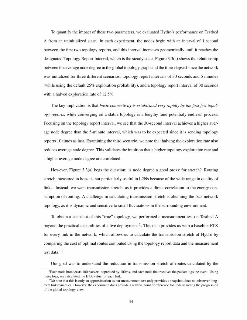
To quantify the impact of these two parameters, we evaluated Hydro’s performance on Testbed
A from an uninitialized state. In each experiment, the nodes begin with an interval of 1 second
between the first two topology reports, and this interval increases geometrically until it reaches the
designated Topology Report Interval, which is the steady state. Figure 3.3(a) shows the relationship
between the average node degree in the global topology graph and the time elapsed since the network
was initialized for three different scenarios: topology report intervals of 30 seconds and 5 minutes
(while using the default 25% exploration probability), and a topology report interval of 30 seconds
with a halved exploration rate of 12.5%.
The key implication is that basic connectivity is established very rapidly by the first few topol-
ogy reports, while converging on a stable topology is a lengthy (and potentialy endless) process.
Focusing on the topology report interval, we see that the 30-second interval achieves a higher aver-
age node degree than the 5-minute interval, which was to be expected since it is sending topology
reports 10 times as fast. Examining the third scenario, we note that halving the exploration rate also
reduces average node degree. This validates the intuition that a higher topology exploration rate and
a higher average node degree are correlated.
However, Figure 3.3(a) begs the question: is node degree a good proxy for stretch? Routing
stretch, measured in hops, is not particularly useful in L2Ns because of the wide range in quality of
links. Instead, we want transmission stretch, as it provides a direct correlation to the energy con-
sumption of routing. A challenge in calculating transmission stretch is obtaining the true network
topology, as it is dynamic and sensitive to small fluctuations in the surrounding environment.
To obtain a snapshot of this “true” topology, we performed a measurement test on Testbed A
beyond the practical capabilities of a live deployment 2. This data provides us with a baseline ETX
for every link in the network, which allows us to calculate the transmission stretch of Hydro by
comparing the cost of optimal routes computed using the topology report data and the measurement
test data. 3
Our goal was to understand the reduction in transmission stretch of routes calculated by the2Each node broadcasts 100 packets, separated by 100ms, and each node that receives the packet logs the event. Using
these logs, we calculated the ETX value for each link.3We note that this is only an approximation as our measurement test only provides a snapshot, does not observer long-
term link dynamics. However, the experiment does provide a relative point of reference for understanding the progressionof the global topology view.
34
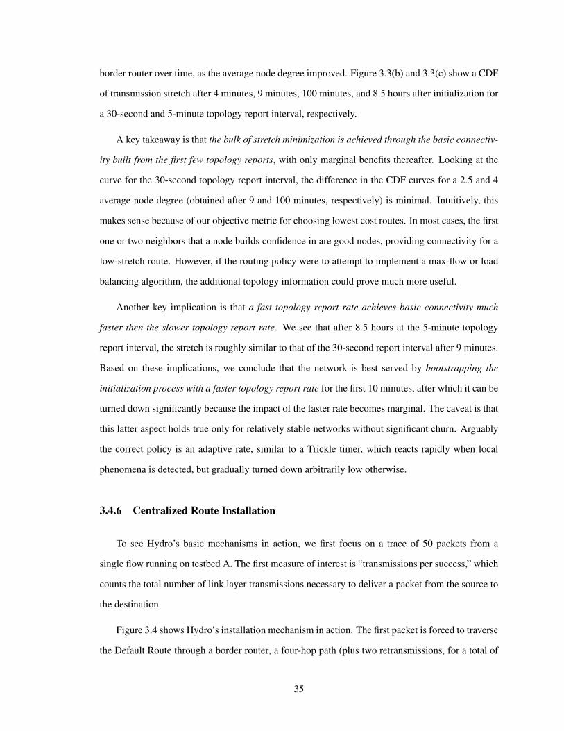
border router over time, as the average node degree improved. Figure 3.3(b) and 3.3(c) show a CDF
of transmission stretch after 4 minutes, 9 minutes, 100 minutes, and 8.5 hours after initialization for
a 30-second and 5-minute topology report interval, respectively.
A key takeaway is that the bulk of stretch minimization is achieved through the basic connectiv-
ity built from the first few topology reports, with only marginal benefits thereafter. Looking at the
curve for the 30-second topology report interval, the difference in the CDF curves for a 2.5 and 4
average node degree (obtained after 9 and 100 minutes, respectively) is minimal. Intuitively, this
makes sense because of our objective metric for choosing lowest cost routes. In most cases, the first
one or two neighbors that a node builds confidence in are good nodes, providing connectivity for a
low-stretch route. However, if the routing policy were to attempt to implement a max-flow or load
balancing algorithm, the additional topology information could prove much more useful.
Another key implication is that a fast topology report rate achieves basic connectivity much
faster then the slower topology report rate. We see that after 8.5 hours at the 5-minute topology
report interval, the stretch is roughly similar to that of the 30-second report interval after 9 minutes.
Based on these implications, we conclude that the network is best served by bootstrapping the
initialization process with a faster topology report rate for the first 10 minutes, after which it can be
turned down significantly because the impact of the faster rate becomes marginal. The caveat is that
this latter aspect holds true only for relatively stable networks without significant churn. Arguably
the correct policy is an adaptive rate, similar to a Trickle timer, which reacts rapidly when local
phenomena is detected, but gradually turned down arbitrarily low otherwise.
3.4.6 Centralized Route Installation
To see Hydro’s basic mechanisms in action, we first focus on a trace of 50 packets from a
single flow running on testbed A. The first measure of interest is “transmissions per success,” which
counts the total number of link layer transmissions necessary to deliver a packet from the source to
the destination.
Figure 3.4 shows Hydro’s installation mechanism in action. The first packet is forced to traverse
the Default Route through a border router, a four-hop path (plus two retransmissions, for a total of
35
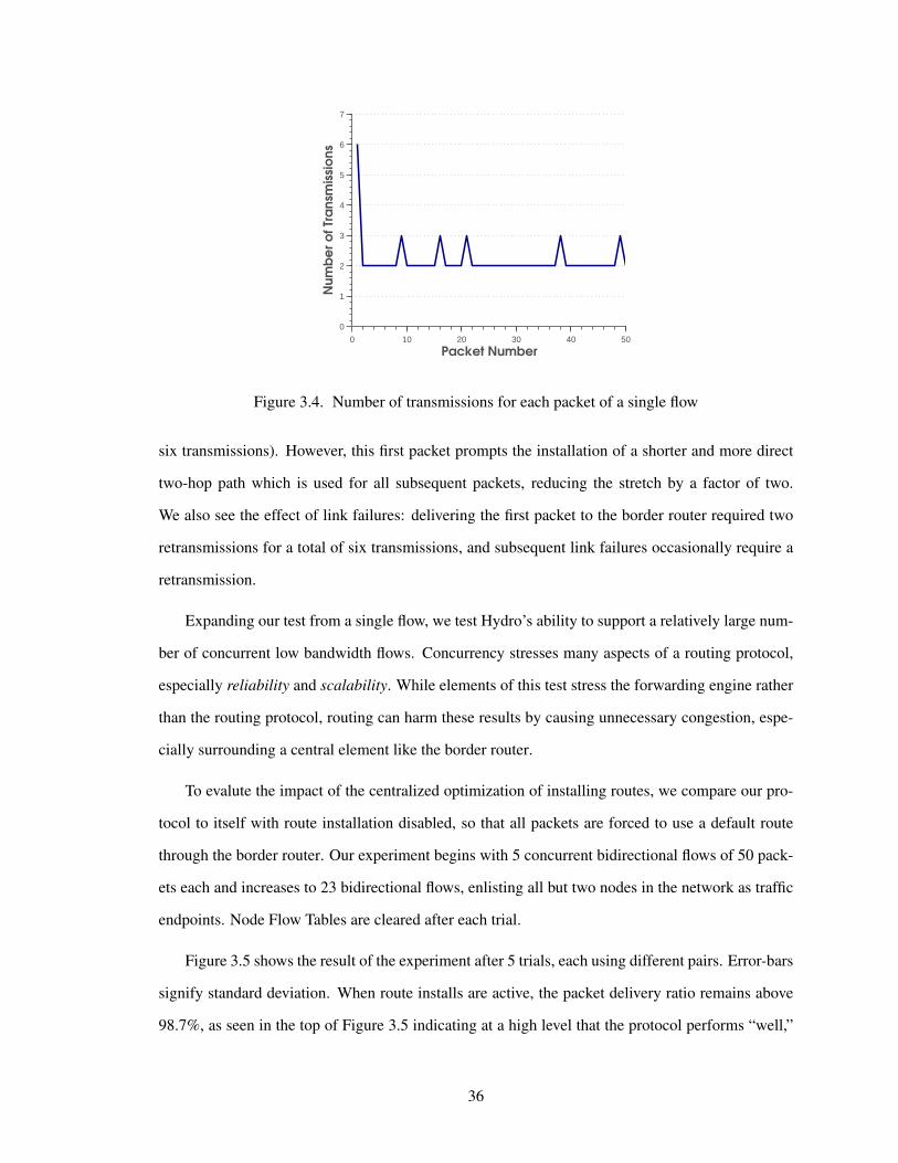
0 10 20 30 40 50
0
1
2
3
4
5
6
7
Packet Number
Nu
mb
er
of Tra
nsm
issio
ns
Figure 3.4. Number of transmissions for each packet of a single flow
six transmissions). However, this first packet prompts the installation of a shorter and more direct
two-hop path which is used for all subsequent packets, reducing the stretch by a factor of two.
We also see the effect of link failures: delivering the first packet to the border router required two
retransmissions for a total of six transmissions, and subsequent link failures occasionally require a
retransmission.
Expanding our test from a single flow, we test Hydro’s ability to support a relatively large num-
ber of concurrent low bandwidth flows. Concurrency stresses many aspects of a routing protocol,
especially reliability and scalability. While elements of this test stress the forwarding engine rather
than the routing protocol, routing can harm these results by causing unnecessary congestion, espe-
cially surrounding a central element like the border router.
To evalute the impact of the centralized optimization of installing routes, we compare our pro-
tocol to itself with route installation disabled, so that all packets are forced to use a default route
through the border router. Our experiment begins with 5 concurrent bidirectional flows of 50 pack-
ets each and increases to 23 bidirectional flows, enlisting all but two nodes in the network as traffic
endpoints. Node Flow Tables are cleared after each trial.
Figure 3.5 shows the result of the experiment after 5 trials, each using different pairs. Error-bars
signify standard deviation. When route installs are active, the packet delivery ratio remains above
98.7%, as seen in the top of Figure 3.5 indicating at a high level that the protocol performs “well,”
36
4 6 8 10 12 14 16 18 20 22 24
0.7
0.75
0.8
0.85
0.9
0.95
1
Pa
ck
et
De
live
ry
Pe
rce
nta
ge
CentralizedTriangle
4 6 8 10 12 14 16 18 20 22 24
0
5
10
15
Ro
ute
In
sta
ll
Tra
ns
(pe
r Fl
ow
)
4 6 8 10 12 14 16 18 20 22 24
0
0.2
0.4
0.6
0.8
Number of Concurrent Flows
DA
G C
on
tro
l P
ac
ke
ts
(pe
r N
od
e)
Figure 3.5. Packet delivery and control traffic rates as a function of the number of concurrent flows,with (centralize) and without (triangle) the route install optimization.
the forwarding engine is “reliable,” and that it supports a reasonably large amount of traffic. The
lower two graphs in Figure 3.5 contain the total number of centralized control transmissions per
flow, and the total DAG maintainence traffic per node per minute. These generally show a low level
of traffic. The kink in the center graph was caused by the protocol reacting to a link failure.
Figures 3.6(a) and 3.6(d) provide additional statistics on the number of transmissions necessary
to deliver packets. We note that the mean number of transmissions necessary to deliver a flow is
stable at slightly more then half of the network diameter, while the number of transmissions per
link indicates Hydrogenerally chooses very reliable links. Even using five trials, there is noticeable
variance in this data due in part to a busy office environment.
When route installs are disabled, the protocol degrades in the face of concurrency. Furthermore,
there is significantly greater variablity without the centralized optimization. We also note that in-
stalling routes reduces stretch, as Figure 3.6(a) illustrates. Testbed A has a diameter of only 3 or 4,
and so the consistent reduction in stretch by one hop is quite significant in relation to the network
diameter.
Centralized systems are often criticized for being too slow to detect and react to remote events.
It is important that the optimization we introduced does not break in the case of node and link
failures. Therefore, we next turn our attention to Hydro’s robustness to node failures. Figure 3.7
examines the performance of a single bidirectional flow as all other nodes in the network are failed.
37
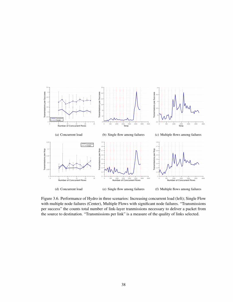
0 5 10 15 20 25
2
2.5
3
3.5
4
4.5
5
5.5
Number of Concurrent Flows
Tra
nsm
issi
on
s p
er
Su
cc
ess
CentralizedTriangle
(a) Concurrent load
0 500 1000 1500 2000 2500 3000 3500
4
6
8
10
12
14
16
Time
Tra
nsm
issi
on
s p
er
Su
cc
ess
(b) Single flow among failures
0 500 1000 1500 2000 2500 3000
2.5
3
3.5
4
4.5
5
Time
Tra
nsm
issi
on
s p
er
Su
cc
ess
(c) Multiple flows among failures
0 5 10 15 20 25
1
1.05
1.1
1.15
1.2
1.25
Number of Concurrent Flows
Tra
nsm
issi
on
s p
er
Ho
p
CentralizedTriangle
(d) Concurrent load
0 500 1000 1500 2000 2500 3000 3500
1.1
1.2
1.3
1.4
1.5
1.6
1.7
1.8
1.9
Number of Concurrent Flows
Tra
nsm
issi
on
s p
er
Ho
p
(e) Single flow among failures
0 500 1000 1500 2000 2500 3000
1
1.1
1.2
1.3
1.4
1.5
1.6
1.7
1.8
Number of Concurrent Flows
Tra
nsm
issi
on
s p
er
Ho
p
(f) Multiple flows among failures
Figure 3.6. Performance of Hydro in three scenarios: Increasing concurrent load (left); Single Flowwith multiple node failures (Center), Multiple Flows with significant node failures. “Transmissionsper success” the counts total number of link-layer tranmissions necessary to deliver a packet fromthe source to destination. “Transmissions per link” is a measure of the quality of links selected.
38
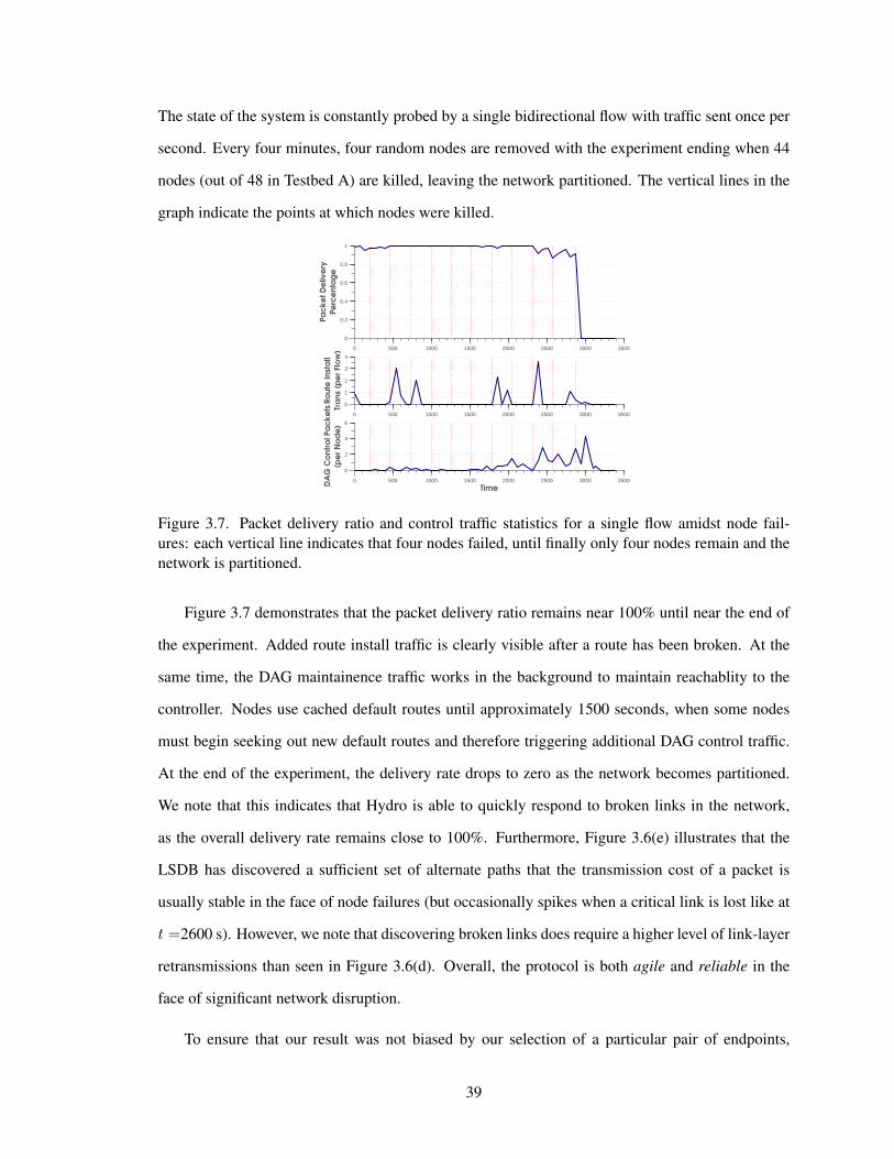
The state of the system is constantly probed by a single bidirectional flow with traffic sent once per
second. Every four minutes, four random nodes are removed with the experiment ending when 44
nodes (out of 48 in Testbed A) are killed, leaving the network partitioned. The vertical lines in the
graph indicate the points at which nodes were killed.
0 500 1000 1500 2000 2500 3000 3500
0
0.2
0.4
0.6
0.8
1
Pa
ck
et
De
live
ry
Pe
rce
nta
ge
0 500 1000 1500 2000 2500 3000 3500
0
1
2
3
4
Ro
ute
In
sta
ll
Tra
ns
(pe
r Fl
ow
)
0 500 1000 1500 2000 2500 3000 3500
0
2
4
6
Time
DA
G C
on
tro
l P
ac
ke
ts
(pe
r N
od
e)
Figure 3.7. Packet delivery ratio and control traffic statistics for a single flow amidst node fail-ures: each vertical line indicates that four nodes failed, until finally only four nodes remain and thenetwork is partitioned.
Figure 3.7 demonstrates that the packet delivery ratio remains near 100% until near the end of
the experiment. Added route install traffic is clearly visible after a route has been broken. At the
same time, the DAG maintainence traffic works in the background to maintain reachablity to the
controller. Nodes use cached default routes until approximately 1500 seconds, when some nodes
must begin seeking out new default routes and therefore triggering additional DAG control traffic.
At the end of the experiment, the delivery rate drops to zero as the network becomes partitioned.
We note that this indicates that Hydro is able to quickly respond to broken links in the network,
as the overall delivery rate remains close to 100%. Furthermore, Figure 3.6(e) illustrates that the
LSDB has discovered a sufficient set of alternate paths that the transmission cost of a packet is
usually stable in the face of node failures (but occasionally spikes when a critical link is lost like at
t =2600 s). However, we note that discovering broken links does require a higher level of link-layer
retransmissions than seen in Figure 3.6(d). Overall, the protocol is both agile and reliable in the
face of significant network disruption.
To ensure that our result was not biased by our selection of a particular pair of endpoints,
39
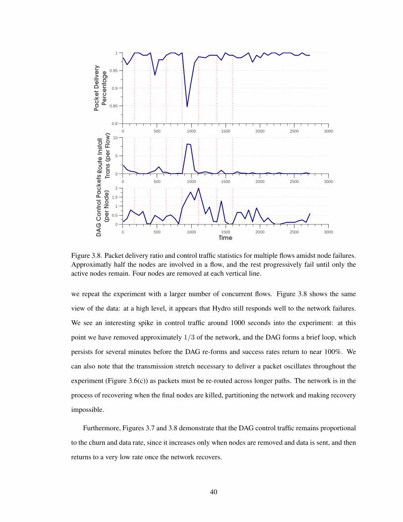
0 500 1000 1500 2000 2500 3000
0.8
0.85
0.9
0.95
1
Pa
ck
et
De
live
ry
Pe
rce
nta
ge
0 500 1000 1500 2000 2500 3000
0
5
10
Ro
ute
In
sta
ll
Tra
ns
(pe
r Fl
ow
)
0 500 1000 1500 2000 2500 3000
0
0.5
1
1.5
2
Time
DA
G C
on
tro
l P
ac
ke
ts
(pe
r N
od
e)
Figure 3.8. Packet delivery ratio and control traffic statistics for multiple flows amidst node failures.Approximatly half the nodes are involved in a flow, and the rest progressively fail until only theactive nodes remain. Four nodes are removed at each vertical line.
we repeat the experiment with a larger number of concurrent flows. Figure 3.8 shows the same
view of the data: at a high level, it appears that Hydro still responds well to the network failures.
We see an interesting spike in control traffic around 1000 seconds into the experiment: at this
point we have removed approximately 1/3 of the network, and the DAG forms a brief loop, which
persists for several minutes before the DAG re-forms and success rates return to near 100%. We
can also note that the transmission stretch necessary to deliver a packet oscillates throughout the
experiment (Figure 3.6(c)) as packets must be re-routed across longer paths. The network is in the
process of recovering when the final nodes are killed, partitioning the network and making recovery
impossible.
Furthermore, Figures 3.7 and 3.8 demonstrate that the DAG control traffic remains proportional
to the churn and data rate, since it increases only when nodes are removed and data is sent, and then
returns to a very low rate once the network recovers.
40
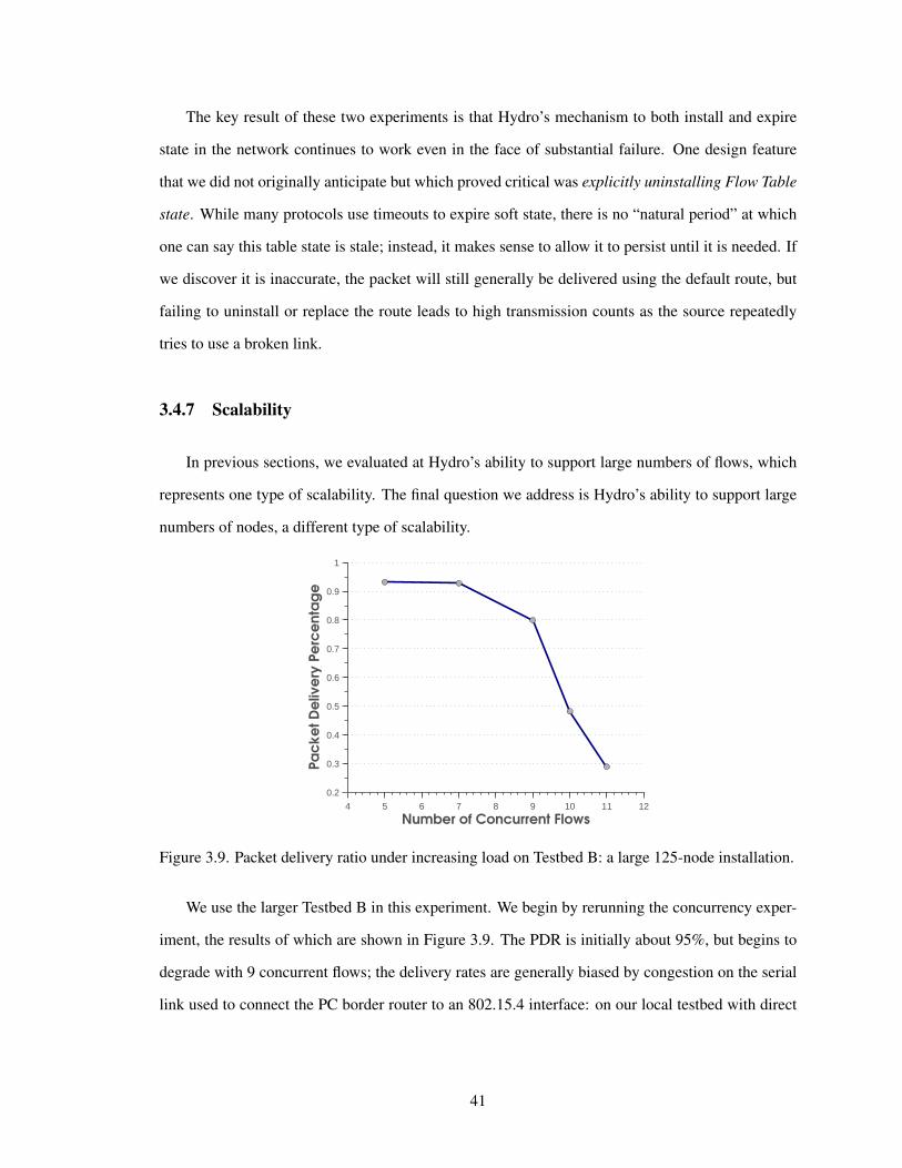
The key result of these two experiments is that Hydro’s mechanism to both install and expire
state in the network continues to work even in the face of substantial failure. One design feature
that we did not originally anticipate but which proved critical was explicitly uninstalling Flow Table
state. While many protocols use timeouts to expire soft state, there is no “natural period” at which
one can say this table state is stale; instead, it makes sense to allow it to persist until it is needed. If
we discover it is inaccurate, the packet will still generally be delivered using the default route, but
failing to uninstall or replace the route leads to high transmission counts as the source repeatedly
tries to use a broken link.
3.4.7 Scalability
In previous sections, we evaluated at Hydro’s ability to support large numbers of flows, which
represents one type of scalability. The final question we address is Hydro’s ability to support large
numbers of nodes, a different type of scalability.
4 5 6 7 8 9 10 11 12
0.2
0.3
0.4
0.5
0.6
0.7
0.8
0.9
1
Number of Concurrent Flows
Pa
ck
et
De
live
ry P
erc
en
tag
e
Figure 3.9. Packet delivery ratio under increasing load on Testbed B: a large 125-node installation.
We use the larger Testbed B in this experiment. We begin by rerunning the concurrency exper-
iment, the results of which are shown in Figure 3.9. The PDR is initially about 95%, but begins to
degrade with 9 concurrent flows; the delivery rates are generally biased by congestion on the serial
link used to connect the PC border router to an 802.15.4 interface: on our local testbed with direct
41
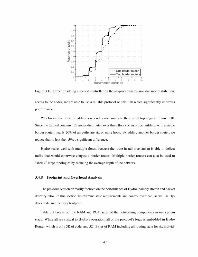
0 1 2 3 4 5 6 7 8 9 10
0
0.1
0.2
0.3
0.4
0.5
0.6
0.7
0.8
0.9
1
Transmission distance
Fra
ctio
n o
f p
airs
One border routerTwo border routers
Figure 3.10. Effect of adding a second controller on the all-pairs transmission distance distribution.
access to the nodes, we are able to use a reliable protocol on this link which significantly improves
performance.
We observe the effect of adding a second border router to the overall topology in Figure 3.10.
Since the testbed contains 128 nodes distributed over three floors of an office building, with a single
border router, nearly 20% of all paths are six or more hops. By adding another border router, we
reduce that to less then 5%, a significant difference.
Hydro scales well with multiple flows, because the route install mechanism is able to deflect
traffic that would otherwise congest a border router. Multiple border routers can also be used to
“shrink” large topologies by reducing the average depth of the network.
3.4.8 Footprint and Overhead Analysis
The previous section primarily focused on the performance of Hydro, namely stretch and packet
delivery ratio. In this section we examine state requirements and control overhead, as well as Hy-
dro’s code and memory footprint.
Table 3.2 breaks out the RAM and ROM sizes of the networking components in our system
stack. While all are critical to Hydro’s operation, all of the protocol’s logic is embedded in Hydro
Router, which is only 5K of code, and 524 Bytes of RAM including all routing state for six individ-
42
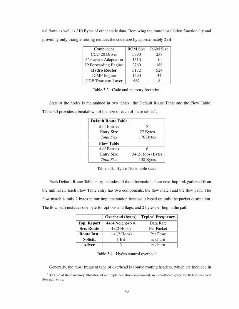
ual flows as well as 210 Bytes of other static data. Removing the route installation functionalty and
providing only triangle routing reduces the code size by approximately 2kB.
Component ROM Size RAM SizeCC2420 Driver 5390 237
6lowpan Adaptation 1310 0IP Forwarding Engine 2760 188
Hydro Router 5172 524ICMP Engine 1590 34
UDP Transport Layer 662 8
Table 3.2. Code and memory footprint.
State at the nodes is maintained in two tables: the Default Route Table and the Flow Table.
Table 3.3 provides a breakdown of the size of each of these tables4.
Default Route Table# of Entries 8Entry Size 22 BytesTotal Size 176 Bytes
Flow Table# of Entries 6Entry Size 3+(2·Hops) BytesTotal Size 138 Bytes
Table 3.3. Hydro Node table sizes
Each Default Route Table entry includes all the information about next-hop link gathered from
the link layer. Each Flow Table entry has two components, the flow match and the flow path. The
flow match is only 2 bytes in our implementation because it based on only the packet destination.
The flow path includes one byte for options and flags, and 2 bytes per hop in the path.
Overhead (bytes) Typical FrequencyTop. Report 4+(4·Neigh)+NA Data RateSrc. Route 4+(2·Hops) Per PacketRoute Inst. 1 + (2·Hops) Per Flow
Solicit. 1 Bit ∝ churnAdver. 3 ∝ churn
Table 3.4. Hydro control overhead
Generally, the most frequent type of overhead is source routing headers, which are included in4Because of static memory allocation of our implementation environment, we pre-allocate space for 10 hops per each
flow path entry.
43
all packets from the border router and also in all packets that use an installed route. We discuss
this limitation in Section 3.6.2. Router solicitations and advertisements also cause a small level of
background traffic; in stable networks these packets are rarely sent, reducing the energy demands of
the protocol.
3.4.9 IETF Criteria
The challenges of serving this class of networks with conventional routing protocols have re-
sulted in an IETF draft that identifies five quantifiable criteria that are necessary for an L2N routing
protocol [40]: We briefly consider these requirements as a check that we have not violated any
well-known design rules for this space.
Table Scalability Each node’s state must be bound by the number of unique destinations it com-
municates with: state in our design is stored only for active flows, and constant size table for
default routes.
Loss Response Any response to loss is localized to the affected data flow: The failure of nodes or
links cause traffic to be diverted to the border router, which is simultaneously alerted of the
change. Fresh state is installed once the border router rebuilds its topology.
Control Cost Control overhead must be bound by the periodic data traffic rate: We have no pe-
riodic beacon traffic. Topology collection is data driven in most cases, and topology reports
are piggybacked on data packets. This traffic involves only the communicating nodes and the
border router.
Link Quality Protocol must define a metric for differentiating among links: Paths are chosen based
on ETX.
Node Cost Protocol must support heterogeneity in the network: Hydro provides the ability for
nodes to specify their willingness to forward packets for other nodes, and node attributes can
be considered in the centralize route computation.
44
3.5 Extensions and Future Work
Hydro consists of a set of primitives for DAG formation, route installation and maintaining the
topology graph in an L2N network, as well as policies and concrete design decisions for how to
use these to develop an optimized unicast routing protocol. Although this paper confines itself to
developing these techniques, the machinery is immediately applicable to several other tasks, which
we develop here.
3.5.1 Multicast Forwarding
Multicast in L2Ns is typically implemented using a message flood where each recipient retrans-
mits a received message exactly once. Although this is generally reliable, epidemic protocols like
Trickle [9] are often also used to ensure that every node hears a multicast message. This basic mech-
anism is somewhat orthogonal to Hydro’s design; it does not address the problem of multicast to a
subset. This is a common task for embedded sensors and actuators, when a large number of nodes
are deployed and a subset needs to be efficiently queried or switched; for example, communicating
with all the lights in a room or all the temperature sensors on a single floor of a building.
Hydro can be used to build efficient support for this by using the global Link State Database
and unicast forwarding. Each node would maintain its own group membership, and report that
information to a border router along with its local topology. To forward a message to a multicast
group, a border router computes the connected components of the subgraph Link State Database
corresponding to the multicast group. It would then unicast the message to a small number of nodes
within each connected component (for reliability); these nodes would then run a dissemination
algorithm like Trickle, where only group members participate.
3.5.2 Policy-Based Routing
It is common in industrial settings for different traffic classes to have different latency and
reliability requirements. For instance, a path part of a control loop may need to maintain a tight
tolerance on jitter, while an alert may need to be delivered as quickly as possible, with no regard to
45
power consumption. On the other hand, it may be acceptable to significantly delay diagnostic data
in order to optimize power consumption.
In order to meet these differing requirement, we envision equipping border routers with multiple
cost functions for path computation, and using traffic class-specific route installations. Since border
routers maintain much of the network link state as well as node attributes for each node router, it
can install inefficient routes for diagnostic data using only mains-powered nodes, while routing alert
and control-loop traffic across the path with the least latency.
3.6 Limitations
Hydro has some important limitations which impact its suitability for some applications.
3.6.1 Adapting to Dynamic Topologies
Hydro can tolerate a certain amount of link and node churn using the mechanisms discussed
in section 3.3.6. However, at some point the network nodes can no longer evaluate links quickly
enough and report them to a border router to allow it to maintain a useful Link State Database.
Although we have observed that Hydro responds well to node and link failure, the protocol is not
designed nor suited for mobile routers. One exception is that routers may use the willingness at-
tribute to indicate that they are willing to forward traffic. This form of “host only” networking
allows mobile nodes to connect to an “infrastructure” formed by a network of static nodes as a leaf
node without disrupting the existing DAG.
3.6.2 Source-Routing in Deep Networks
The use of source routing comes with the well-known limitation of per-packet overhead. Despite
this limitation, we chose to use it for its key advantage of loop-freedom. None the less, full source
routes become impractical in very deep networks. We felt that our protocol is be adequate for our
needs since it supports multiple border routers, which we use to reduce the number of hops a packet
must be source routed across with a minimum of complexity. However, some domains require very
46
deep networks. Hydro uses source routes in two places: for routing into the subnet from border
routers, and for installed routes. Removing each of these is a challenge, since there is the potential
for significant state complexity as well as loops.
In order to allow packets to be sent into the network from a border router without a source
route, one technique is for each node in the network to maintain a list of nodes upstream from it in
the DAG; this is similar to the technique employed in TBRPF [41]. However, it also introduces a
requirement for a table as large as the number of nodes in the network; we view this as unacceptable.
To remedy this problem, the protocol could choose clusterheads or waypoints in the graph and then
define loose source routes between them; this technique effectively compresses a source route.
Choosing and maintaining this subset of set waypoints is likely to pose a challenge in the face of
network dynamics, and increases implementation complexity.
An installed route may take advantage of waypoints if available to compress routes; additionally
(or alternatively), a route may be installed at each hop as is often done in other centralized routing
solutions. However, this introduces the potential for routing loops when an node along a path fails
or looses its state. This failure mode can be resolved by caching packet signatures, so as to be able
to quickly identify when a packet has encountered a loop without waiting for TTL expiry.
3.6.3 Single Point of Congestion/Failure
Each border router represents a substantial amount of state which has been accumulated by
the border router. Furthermore, high traffic loads congest the medium around border routers. We
admit that these are problem, but argue that they are ameliorated by realities of L2N deployment.
First, since a border router typically also functions as an egress point, its failure typically termi-
nates data collection regardless of the state of the routing protocol. Secondly, congestion of the
medium indicates poor capacity planning, and should remedied through through additional capacity
deployment.
47
Chapter 4
Example Deployemnt: AC Metering
4.1 Overview
Sensor network research has made great progress over the past decade in creating low-power
wireless embedded devices, systems, and networking technology, and this technology has been
applied to numerous studies of real-world environments. Many of these, including habitat and
climate monitoring demand extremely low energy consumption, long lifetime on batteries, low
sample rates, and reliable ad-hoc networking in wide open spaces. In this paper we focus on a large
scale wireless sensor network for a very different kind of application– high fidelity, building-wide,
electricity monitoring.
Electricity usage in residential and commercial buildings represent a significant fraction of total
energy expenditure and, since electricity is generated from fossil fuels, it represents a significant
portion of the carbon footprint of the occupant. The typical Pacific Gas & Electric (PG&E) customer
uses about 540kWh of electricity per month, while the Computer Science Division building at the
authors’ institution consumes approximately 12MWh of electricity per day. This usage is divided
between HVAC, lighting, plug-loads, and servers. Preliminary data show that the plug-load usage
represents approximately 20%, or 2.4MWh, of the total usage and that much of this is desktop
systems. In addition, these loads generate heat that must be removed by the HVAC system. Desktop
usage is also highly correlated with lighting loads. Our goal is to build an interactive, near real-time
48
monitoring capability of numerous small loads, as well as the fewer large ones, so that occupants can
understand their electricity usage patterns and adapt their behavior to reduce their energy footprint.
The AC metering application drives a different set of technical challenges and pushes sensor
network research in some new directions. Although ultra low power operation on batteries is not
required, since the embedded devices are mains-powered, they must consume little enough energy
that they do not adversely affect the standby monitoring load. Moreover, since they are monitoring
the very flow of electricity that they utilize, so the design of the AC-DC power supply and the power
metering is inter-related and rather subtle. The design of the embedded device must address a family
of thermal, noise isolation, and safety concerns that few sensor networks have examined. We use
this challenge to exercise the recently published Epic [42] design methodology of expert modules
and application-specific “glue” to support the progression from prototype to pilot to production.
While the network need not operate with a low radio duty cycle, it needs to be robust even though
the devices are deployed in highly RF challenged settings – behind refrigerators, under metal desks,
in metal cabinets, on the microwave, and so on.
Moreover, the collection of devices is not a distributed instrument deployed by a single author-
ity, i.e., a macroscope; rather, it is a network deployed bottom up by individuals for a variety of
reasons in a variety of settings. The application and usage can be quite heterogeneous, although all
the devices cooperate at the network layer to route traffic for one another. This application is one
the first deployments of a new, open source IPv6 network stack over 802.15.4 using 6LoWPAN.
All of the routing on the motes is true IP routing and a collection of modified Meraki Mini nodes
route between the 6LoWPAN subnet and the various other subnets. This enables a distribution,
deployment, management, and data analysis model that is essentially that of a distributed collection
of hosts: some clients, some servers, some both.
To evaluate our design, we apply the technology to the problem of excessive energy usage in
our Computer Science Building. In this project, we made ACme nodes available to a relatively
large number of students, faculty, and staff, and encouraged them to monitor their workstations,
laptops, and other electronics. Collectively the data collection occurs over our ad-hoc mesh network.
We have also instrumented other devices with significant power draw in common areas, and made
complete power traces from these devices publicly available via the database and web interface.
49
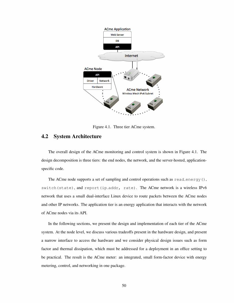
Figure 4.1. Three tier ACme system.
4.2 System Architecture
The overall design of the ACme monitoring and control system is shown in Figure 4.1. The
design decomposition is three tiers: the end nodes, the network, and the server-hosted, application-
specific code.
The ACme node supports a set of sampling and control operations such as read energy(),
switch(state), and report(ip addr, rate). The ACme network is a wireless IPv6
network that uses a small dual-interface Linux device to route packets between the ACme nodes
and other IP networks. The application tier is an energy application that interacts with the network
of ACme nodes via its API.
In the following sections, we present the design and implementation of each tier of the ACme
system. At the node level, we discuss various tradeoffs present in the hardware design, and present
a narrow interface to access the hardware and we consider physical design issues such as form
factor and thermal dissipation, which must be addressed for a deployment in an office setting to
be practical. The result is the ACme meter: an integrated, small form-factor device with energy
metering, control, and networking in one package.
50
A set of disconnected meters is much less interesting than real-time data. Traditional monitoring
designs use sneakernet and a small LCD, a serial port, or other wired ports connecting instruments to
data loggers. A key motivation of our work is to allow the quick deployment and instrumentation of
a large numbers of AC plug meters and enable continuous real-time access. Requiring connectivity
over USB, serial, Ethernet, or other wired channel would not be practical. Also, although most
places we wish to measure have substantial 802.11 infrastructure installed, the reality is that it is
not easy to add additional devices to these networks. Thus, our solution is the development of an
ad-hoc IEEE 802.15.4 network layer that provides IP connectivity to ACme nodes without the use
of either wiring or infrastructure. The network provides connectivity between the sensor nodes and
other networks using a dual-interface router.
Finally, application specific code can be placed on any network connected to the ACme meter
subnet. Applications use the node API as exported over the network. Typically, a server daemon
populates a database that is accessed by a variety of web applications, but direct access to ACme
including telnet and a UDP RPC is available as well. We present a green building power profiling
application which allows users to view their individual real-time energy consumption using a web
interface. It consists of a logger daemon which formats and inserts the reported data into a database,
and a presentation layer which synthesizes reports from this logged data. A key architectural sepa-
ration is that applications are developed independently from the network used.
4.3 ACme Network
Unlike sensor networks with carefully controlled node placements to ensure good connectivity,
users may install their ACme meters under their desks, behind metal filing cabinets, or in metal floor
boxes, and expect that their data will be visible online. Coverage of these locations by Wi-Fi access
points is typically difficult. Instead we utilize the high density of these nodes and multihop routing
to obtain coverage, even with milliwatt power radios. Their relatively low, packet-per-minute data
rates can be serviced by a 802.15.4 mesh.
51
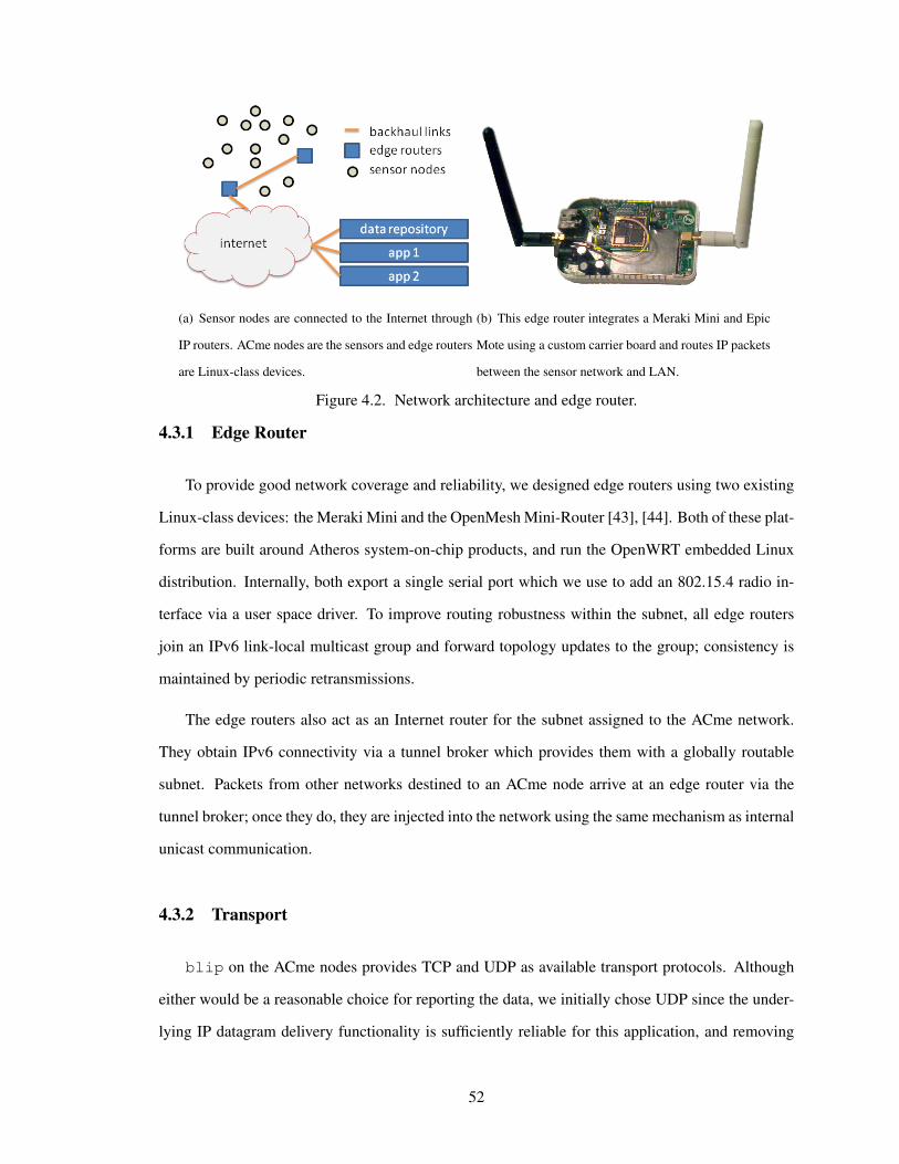
(a) Sensor nodes are connected to the Internet through
IP routers. ACme nodes are the sensors and edge routers
are Linux-class devices.
(b) This edge router integrates a Meraki Mini and Epic
Mote using a custom carrier board and routes IP packets
between the sensor network and LAN.
Figure 4.2. Network architecture and edge router.
4.3.1 Edge Router
To provide good network coverage and reliability, we designed edge routers using two existing
Linux-class devices: the Meraki Mini and the OpenMesh Mini-Router [43], [44]. Both of these plat-
forms are built around Atheros system-on-chip products, and run the OpenWRT embedded Linux
distribution. Internally, both export a single serial port which we use to add an 802.15.4 radio in-
terface via a user space driver. To improve routing robustness within the subnet, all edge routers
join an IPv6 link-local multicast group and forward topology updates to the group; consistency is
maintained by periodic retransmissions.
The edge routers also act as an Internet router for the subnet assigned to the ACme network.
They obtain IPv6 connectivity via a tunnel broker which provides them with a globally routable
subnet. Packets from other networks destined to an ACme node arrive at an edge router via the
tunnel broker; once they do, they are injected into the network using the same mechanism as internal
unicast communication.
4.3.2 Transport
blip on the ACme nodes provides TCP and UDP as available transport protocols. Although
either would be a reasonable choice for reporting the data, we initially chose UDP since the under-
lying IP datagram delivery functionality is sufficiently reliable for this application, and removing
52
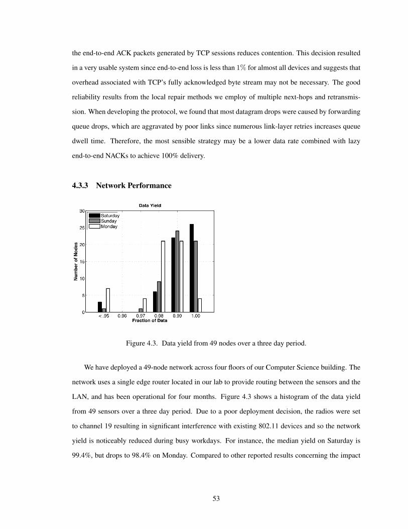
the end-to-end ACK packets generated by TCP sessions reduces contention. This decision resulted
in a very usable system since end-to-end loss is less than 1% for almost all devices and suggests that
overhead associated with TCP’s fully acknowledged byte stream may not be necessary. The good
reliability results from the local repair methods we employ of multiple next-hops and retransmis-
sion. When developing the protocol, we found that most datagram drops were caused by forwarding
queue drops, which are aggravated by poor links since numerous link-layer retries increases queue
dwell time. Therefore, the most sensible strategy may be a lower data rate combined with lazy
end-to-end NACKs to achieve 100% delivery.
4.3.3 Network Performance
Figure 4.3. Data yield from 49 nodes over a three day period.
We have deployed a 49-node network across four floors of our Computer Science building. The
network uses a single edge router located in our lab to provide routing between the sensors and the
LAN, and has been operational for four months. Figure 4.3 shows a histogram of the data yield
from 49 sensors over a three day period. Due to a poor deployment decision, the radios were set
to channel 19 resulting in significant interference with existing 802.11 devices and so the network
yield is noticeably reduced during busy workdays. For instance, the median yield on Saturday is
99.4%, but drops to 98.4% on Monday. Compared to other reported results concerning the impact
53
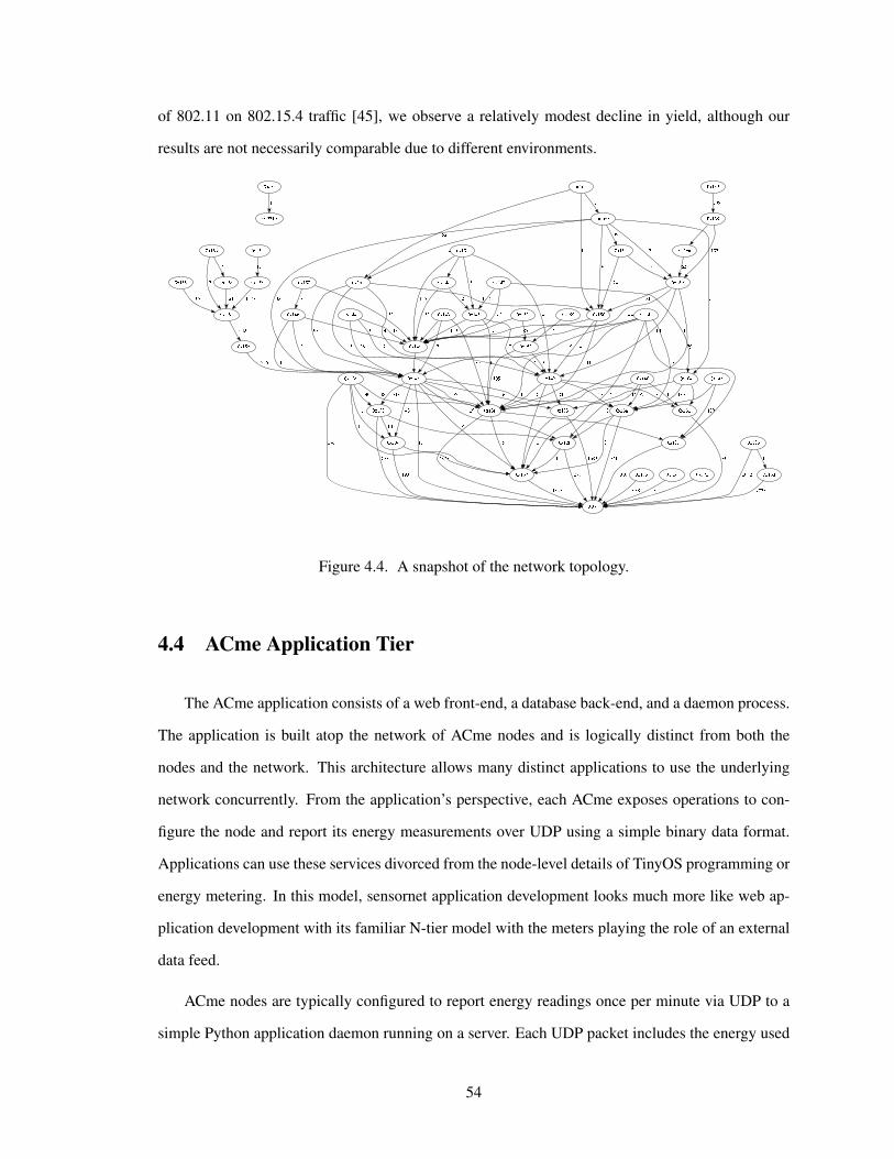
of 802.11 on 802.15.4 traffic [45], we observe a relatively modest decline in yield, although our
results are not necessarily comparable due to different environments.
Figure 4.4. A snapshot of the network topology.
4.4 ACme Application Tier
The ACme application consists of a web front-end, a database back-end, and a daemon process.
The application is built atop the network of ACme nodes and is logically distinct from both the
nodes and the network. This architecture allows many distinct applications to use the underlying
network concurrently. From the application’s perspective, each ACme exposes operations to con-
figure the node and report its energy measurements over UDP using a simple binary data format.
Applications can use these services divorced from the node-level details of TinyOS programming or
energy metering. In this model, sensornet application development looks much more like web ap-
plication development with its familiar N-tier model with the meters playing the role of an external
data feed.
ACme nodes are typically configured to report energy readings once per minute via UDP to a
simple Python application daemon running on a server. Each UDP packet includes the energy used
54
in the previous minute as well as the average, minimum, and maximum instantaneous power ob-
served during the same interval. The daemon parses the UDP packets, extracts the relevant readings,
timestamps the data, checks for duplicate data, and inserts the readings into a MySQL database.
Users access historical energy data through a web interface that queries the database and presents
the results in tabular and graphical form. Although most queries access archival data, the system
also allows users to control plug-loads registered to them by switching power to them (this function
is not exposed in the user interface). In this case, the web application can directly send a command
to the node.
This application architecture marks a departure from interacting with the sensor network in the
aggregate to interacting with the individual nodes themselves as IP endpoints. This approach pro-
vides an opportunity to leverage standard networking tools and libraries like ping, wireshark,
and netcat to monitor the nodes, debug networking problems, and build applications.
Since this architecture eliminates the application-layer gateway and the proxy role the gateway
plays in the process, the architecture raises new concerns. Allowing unbridled IP network access to
sensor nodes raises many security challenges, and they are likely to be more pressing since the nodes
are resource-constrained. Techniques like NATs, firewalls, and policy-aware switching already exist
to solve these problems in existing enterprise networks and they may also be applicable here.
4.5 Related Work
Virtually all households in the United States have electric meters installed. Unfortunately, the
data they provide is not very useful for either identifying per-appliance energy consumption or
generating real-time feedback of usage because of the low sample rates and lack of network con-
nections. Work in this area has resulted in “smart meters,” which replace traditional analog meters
and are able to report usage data to a utility at a much finer temporal granularity then previously
available. However, these meters do not extend within residences to provide the fine-grain view we
provide.
With the recent increase of awareness in energy conservation, several commercial products
have appeared on the market which measure single outlet energy consumption, commonly referred
55

to as plug-load meters [46]. These are helpful for point measurements, but still require manual
measurement. Such an approach does not address the deployment challenges at scale, which our
solution addresses directly.
Several startups, such as Tendril [47], GreenBox [48], and EnergyHub [49], have recently an-
nounced proprietary wireless monitoring solutions that are not yet publicly available. Their tech-
nology is similar to ours, and provides an interesting parallel in the closed space.
A few sensor network systems have explored AC metering including MIT’s “Plug” plat-
form [50]. “Plug” provides apparent power measurements through a current transformer and uses
an ADC for direct sampling. This design choice was discussed in this project but not used due to
its size, lack of real and reactive power, and lack of energy accumulation. Microsoft Research’s
“smart-socket” [51] uses a similar design as ACme but is battery-powered. Their web services ap-
proach interoperates with other sensors and control points, and their results shows energy savings
in a home context, but their focus is on application composition.
High fidelity power measurement is also very important. Several studies have looked at using
high fidelity power traces to identify appliances and their states [52]–[54]. High fidelity data can
also be used for fault detection [55], power grid health monitoring and fault forecasting [56].
4.6 Discussion
Energy applications drive the sensor network research agenda in new directions with different
requirements and constraints. Power, for example, while no longer being a constraint, is still very
intertwined with the design. The network architecture and protocols are still limited by low band-
widths and small memories, but are now required to provide support for different traffic patterns
than those used in traditional sensor networks. Finally, while radio connectivity is still an important
part of design, the focus switches from designing extremely low duty-cycle media access protocols
to coping with the crowded environment found indoors.
The natural evolution of this work is to move metering from a separate device into the appli-
ance. Cost is an important constraint on the types of devices which will find favor, and for this
56

reason the metering devices will still have very inexpensive microcontrollers and low-power radios,
although appliances may export more functionality than is present in our design. Critically, power
applications will require a general purpose network rather than specialized protocols and application
gateways. Future research may integrate programmability into the end devices to allow them to be
tasked with more elaborate data processing and generation tasks than our current model allows.
57
Chapter 5
Conclusions
Throughout the design of blip we have striven to make it as simple and straightforward for
application developers; decisions like providing an easy-to-extend shell component and designing
the transport-layer interfaces to remove a requirement for complicated application buffering strate-
gies seem to have importantly reduced the amount of code developers must write; simple yet useful
applications consist of little more then a UDP socket and a timer. The design of Hydro has also
had an impact outside of academia, through our involvement in the IETF process for standardizing
routing over this class of lossy, low-power networks. Some of the design experiences from Hydro
have been incorporated into work on the routing protocol for the sensor tier of the Internet, RPL.
Looking forward, blip will continue to be an important component of the Berkeley stable of
sensor technology. We are currently in the process of fitting Cory Hall, the Electrical Engineering
building here at UC Berkeley with dense instrumentation; we also working towards a deployment
of hundreds more nodes in collaboration with Lawrence Berkeley National Laboratory. These ex-
periences have for the most part validated the design decisions made in blip, but also pointed
out places where it falls short. In particular, there has been little work so far on application-layer
protocols running on top of an IP stack appropriate for sensing application; we are just beginning to
address this important problem with recent work in our group.
Projects either evolve or die; our hope is that blip will do the former. It is currently in
transition, as IETF work on standardization is coming closer to convergence and external users
58
begin to play a more important role in its development. We have begun the development of the next
major release of the project, which will support the lastest standards and also demonstrate prototype
implementations of RPL and PIM running over low-power networks.
From a research point of view, applying the IP architecture answers a host of questions but
leaves another set of questions untouched. In particular, the embedded community still does not
have a satisfactory Media Access Protocol for low-power operation despite a decade of research.
We feel that the problem is mostly an issue of lack of implementation effort rather then techno-
logical fundamentals, since there exist commercial protocols which appear to have satisfactory per-
formance. We are closing on a release of A-MAC, a protocol developed in collaboration with
Prabal Dutta that offers an attractive power envelope and good performance over a wide range of
workloads; it outperforms open implementations of both receiver-initiated (RI-MAC) and sampling-
based (BoX-MAC) protocols in most areas [57], [58]. Unfortunately these results were not ready in
time for this manuscript.
Now that the IP architecture will most likely be adopted and take over in yet another network
tier, researchers must look further down the road to continue to push the limits. Most immediately,
there is a need for application protocols which integrate well with existing Internet architecture, yet
are also amenable to efficient low-power operation. In particular, design lessons from 6lowpan,
where protocol-specific adaptations are made to reduce payload size or the frequency of messages
may need to be applied further up the stack; the CORE working group at the IETF would surely
benefit from some clarifying design work from Academia. Further down the road, energy harvesting
and its impacts on all levels of the stack appears to be relatively fresh territory, since there are not
well-known techniques for adapting to variability in energy supply.
59
References
[1] R. Braden, “RFC 1122: Requirements for internet hosts – communication layers,” 1989.[2] J. Hui and D. Culler, “Ip is dead, long live ip for wireless sensor networks,” in the 6th ACM Conference on Embedded
Networked Sensor Systems (SenSys), 2008.[3] J. Moy, “RFC 2178: Ospf version 2,” 1998.[4] D. Oran, “RFC 1142: Osi is-is intra-domain routing protocol,” 1990.[5] P. Levis, A. Tavakoli, and S. Dawson-Haggerty, “Overview of existing routing protocols for low power and lossy
networks,” in IETF Internet Draft, 2009.[6] I. D. Chakeres and C. E. Perkins, “Dynamic manet on-demand (dymo) routing (work in progress: draft-ietf-manet-
dymo-10),” 2007.[7] Y. Mao, F. Wang, L. Qiu, S. Lam, and J. Smith, “S4: Small state and small stretch routing protocol
implementation.” [Online]. Available: http://www.cs.utexas.edu/∼lili/projects/s4.htm[8] R. Fonseca, O. Gnawali, K. Jamieson, and P. Levis, “Collection tree protocol,” http://www.tinyos.net/tinyos-
2.x/doc/html/tep119.html.[9] P. Levis, N. Patel, D. Culler, and S. Shenker, “Trickle: A self-regulating algorithm for code maintenance and
propagation in wireless sensor networks,” in First USENIX/ACM Symposium on Network Systems Design and Im-plementation (NSDI), 2004.
[10] S. Deering and R. Hinden, “RFC 2460: Internet protocol, version 6 (ipv6) specification,” 1998.[11] T. Narten, “Neighbor discovery and stateless autoconfiguration in ipv6,” IEEE Internet Computing, vol. 3, no. 4,
pp. 54–62, 1999.[12] G. Montenegro, N. Kushalnagar, J. Hui, and D. Culler, “RFC 4944: Transmission of ipv6 packets over ieee 802.15.4
networks,” 2007.[13] A. Dunkels, “Tcp/ip for 8-bit architectures,” in In Proceedings of The First International Conference on Mobile
Systems, Applications, and Services (MOBISYS 03, 2003.[14] M. Maroti, B. Kusy, G. Simon, and Akos Ledeczi, “The flooding time synchronization protocol,” in SenSys ’04:
Proceedings of the 2nd international conference on Embedded networked sensor systems. New York, NY, USA:ACM Press, 2004, pp. 39–49.
[15] G. Tolle, J. Polastre, R. Szewczyk, D. Culler, N. Turner, K. Tu, S. Burgess, T. Dawson, P. Buonadonna, D. Gay, andW. Hong, “A macroscope in the redwoods,” ACM Sensys, 2005.
[16] X. Jiang, S. Dawson-Haggerty, P. Dutta, and D. Culler, “Design and implementation of a high-fidelity ac meteringnetwork,” in Proceedings of the 8th ACM/IEEE International Conference on Information Processing in SensorNetworks (IPSN’09) Track on Sensor Platforms, Tools, and Design Methods, 2009.
[17] G. Werner-Allen, K. Lorincz, J. Johnson, J. Lees, and M. Welsh, “Fidelity and yield in a volcano monitoring sensornetwork,” in OSDI, 2006, pp. 381–396.
[18] A. Woo, T. Tong, and D. Culler, “Taming the underlying challenges of multihop routing in sensor networks,” inProceedings of the First ACM Conference on Embedded Networked Sensor Systems, Los Angeles, CA, Nov. 2003.
[19] T. Stathopoulos, L. Girod, J. Heideman, D. Estrin, and K. Weeks, “Centralized routing for resource-constrainedwireless sensor networks (sys 5),” 2006. [Online]. Available: http://research.cens.ucla.edu/pls/portal/url/item/20A76F675835AB5DE0406180528D2E28
[20] O. Gnawali, B. Greenstein, K.-Y. Jang, A. Joki, J. Paek, M. Vieira, D. Estrin, R. Govindan, and E. Kohler, “Thetenet architecture for tiered sensor networks,” ACM Sensys, 2006.
[21] R. Musaloiu-E., C.-J. M. Liang, and A. Terzis, “Koala: Ultra-low power data retrieval in wireless sensor networks,”International Conference on Information Processing in Sensor Networks, vol. 0, pp. 421–432, 2008.
[22] K. S. J. Pister and L. Doherty, “Tsmp: Time synchronized mesh protocol,” in Parallel and Distributed Computerand Systems, 2008.
[23] R. Fonseca, S. Ratnasamy, D. Culler, S. Shenker, and I. Stoica, “Beacon vector routing: Scalable point-to-pointrouting in wireless sensornets,” in In NSDI, 2005.
[24] Y. Mao, F. Wang, L. Qiu, S. S. Lam, and J. M. Smith, “S4: Small state and small stretch routing protocol for largewireless sensor networks,” in NSDI, 2007.
[25] J. Ortiz, C. R. Baker, D. Moon, R. Fonseca, and I. Stoica, “Beacon location service: A location service for point-to-point routing in wireless sensor networks,” in International Conference in Information Processing in SensorNetworks: Special Track on Platform Tools and Design Methods for Network Embedded Sensors, 2007.
[26] C. E. Perkins and E. M. Belding-Royer, “Ad-hoc on-demand distance vector routing,” in WMCSA, 1999, pp. 90–100.
60
[27] D. Johnson, Y. Hu, and D. Maltz, “RFC 4728: The dynamic source routing protocol (dsr) for mobile ad hoc networksfor ipv4,” 2007.
[28] T. Clausen and P. Jacquet, “RFC 3626: Optimized link state routing protocol,” 2003.[29] M. Bahr, “Proposed routing for ieee 802.11s wlan mesh networks,” in WICON ’06: Proceedings of the 2nd annual
international workshop on Wireless internet. New York, NY, USA: ACM, 2006, p. 5.[30] M. Casado, M. J. Freedman, J. Pettit, J. Luo, and N. Mckeown, “Ethane: Taking control of the enterprise,” in
SIGCOMM Computer Comm. Rev, 2007.[31] N. Feamster, H. Balakrishnan, J. Rexford, A. Shaikh, and K. van der Merwe, “The Case for Separating Routing
from Routers,” in ACM SIGCOMM Workshop on Future Directions in Network Architecture (FDNA), Portland, OR,September 2004.
[32] M. Caesar, D. Caldwell, N. Feamster, J. Rexford, A. Shaikh, and J. van der Merwe, “Design and implementation ofa routing control platform,” in NSDI’05: Proceedings of the 2nd conference on Symposium on Networked SystemsDesign & Implementation. Berkeley, CA, USA: USENIX Association, 2005, pp. 15–28.
[33] A. Greenberg, G. Hjalmtysson, D. A. Maltz, A. Myers, J. Rexford, G. Xie, H. Yan, J. Zhan, and H. Zhang, “A cleanslate 4d approach to network control and management,” vol. 35. New York, NY, USA: ACM, 2005, pp. 41–54.
[34] H. Yan, D. A. Maltz, T. S. E. Ng, H. Gogineni, H. Zhang, and Z. Cai, “Tesseract: A 4d network control plane,” inIn ACM/USENIX NSDI, 2007.
[35] K. Srinivasan, P. Dutta, A. Tavakoli, and P. Levis, “Understanding the causes of packet delivery success and fail-ure in dense wireless sensor networks,” Technical Report SING-06-00, Computer Science Department, StanfordUniversity, 2006.
[36] P. Levis, S. Madden, J. Polastre, R. Szewczyk, K. Whitehouse, A. Woo, D. Gay, J. Hill, M. Welsh, E. Brewer, andD. Culler, “Tinyos: An operating system for wireless sensor networks,” Ambient Intelligence, 2005.
[37] “Chipcon cc24020. cc2420 2.4 ghz ieee 802.15.4/zigbee-ready rf transceiver.” http://www.chipcon.com.[38] “Micaz,” http://www.xbow.com/Products/Product pdf files/Wireless pdf/MICAz Datasheet.pdf.[39] J. Polastre, R. Szewczyk, and D. Culler, “Telos: Enabling ultra-low power wireless research,” IEEE SPOTS, 2005.[40] P. Levis, A. Tavakoli, and S. Dawson-Haggerty, “Overview of existing routing protocols for low power and lossy
networks,” 2008.[41] R. Ogier, F. Templin, and M. Lewis, “RFC 3684:topology dissemination based on reverse-path forwarding (tbrpf),”
United States, 2004.[42] P. Dutta, J. Taneja, J. Jeong, X. Jiang, and D. Culler, “A building block approach to sensornet systems,” in SenSys,
2008.[43] “Meraki, inc.” http://www.meraki.com.[44] “Open mesh mini-router.” http://www.open-mesh.com.[45] R. Musaloiu-E. and A. Terzis, “Minimising the effect of wifi interference in 802.15.4 wireless sensor networks,”
Int. J. Sen. Netw., vol. 3, no. 1, pp. 43–54, 2007.[46] “Kill-a-watt,” http://www.p3international.com/products/special/P4400/P4400-CE.html.[47] “Tendril,” http://www.tendrilinc.com/.[48] “Green box,” http://www.getgreenbox.com/.[49] “Green hub,” http://www.energyhub.net/.[50] J. Lifton, M. Feldmeier, Y. Ono, C. Lewis, and J. A. Paradiso, “A platform for ubiquitous sensor deployment
in occupational and domestic environments,” in IPSN ’07: Proceedings of the 6th international conference onInformation processing in sensor networks. New York, NY, USA: ACM, 2007, pp. 119–127.
[51] B. Priyantha, A. Kansal, M. Goraczko, and F. Zhao, “Tiny web services: Design and implementation on interoper-able and evolvable sensor networks,” in ACM/IEEE Conference on Embedded Networked Sensor Systems (SenSys’08), 2008.
[52] M. Ito, R. Uda, S. Ichimura, K. Tago, T. Hoshi, and Y. Matsushita, “A method of appliance detection based onfeatures of power waveform,” Applications and the Internet, IEEE/IPSJ International Symposium on, vol. 0, p. 291,2004.
[53] C. Laughman, K. Lee, R. Cox, S. Shaw, S. Leeb, L. Norford, and P. Armstrong, “Power signature analysis,” IEEEPower & Energy Magazine, 2003.
[54] W. Lee, G. Fung, H. Lam, F. Chan, and M. Lucente, “Exploration on load signatures,” International Conference onElectrical Engineering (ICEE), 2004.
[55] M. E. H. Benbouzid, “A review of intruction motors signature analysis as a medium for faults detection.” IEEETransactions on Industrial Electronics, 47(5), 2000.
61

[56] P. Ge, Q. Guo, H. Zhou, X. Li, W. Xu, G. Tang, and Q. Xu, “Wide area power grid health state diagnosis and earlywarning system based on fault power flow fingerprint identification and mas technology,” DRPT2008, 2008.
[57] Y. Sun, O. Gurewitz, and D. B. Johnson, “RI-MAC: a receiver-initiated asynchronous duty cycle mac protocol fordynamic traffic loads in wireless sensor networks,” in Proceedings of the 6th International Conference on EmbeddedNetworked Sensor Systems, SenSys 2007, Raleigh, NC, USA, November 5-7, 2008, 2008, pp. 1–14.
[58] D. Moss and P. Levis, “BoX-MACs: Exploiting Physical and Link Layer Boundaries in Low-Power Networking,”Stanford Information Networks Group, Tech. Rep. SING-08-00, 2008.
62