design of a primary off-gas scrubber system for a ferro
TRANSCRIPT

Design of a primary off-gas scrubber for a
ferro-manganese electric arc furnace process
JP Fourie
21109990
Dissertation submitted in fulfilment of the requirements for the
degree Magister in Chemical Engineering at the Potchefstroom
Campus of the North-West University
Supervisor: Prof FB Waanders
November 2014

1
Acknowledgements First and foremost I would like to thank our Heavenly Father, from whom my help comes. His grace
alone has granted me the capability of furthering my studies in the form of this dissertation.
I would also like to express my sincere gratitude to my advisor Prof. Frans Waanders, for affording me
this opportunity and his continuous support during my research. His guidance as a mentor is
unparalleled; I have gained wisdom and knowledge both professionally and personally, for which I will
always be grateful.
I thank my loving wife Sanri, who has been a pillar of support, even during the most demanding times
of my research. She has been a well of motivation and encouragement; truly a blessing.
In loving memory of my late father Danie, who instilled in me the value of integrity and persistence. I
would not have been able to appreciate this opportunity without his guidance; he would have been
proud.
Last but not least, I would like to thank my mother Joy and my sister Natasha, who have always been
supportive of my efforts. Knowing that someone believes in you is often all you need to achieve
success.

Design of a primary off-gas scrubbing system for a ferromanganese electric arc furnace process
Jethro P. Fourie*
School for Chemical Engineering, North-West university, Potchefstroom, 2520, South Africa
ABSTRACT
An electric arc furnace makes use of electrical energy in the form of an arc to heat charged material. In the
ferromanganese smelting process the ferric oxide (Fe2O3) and manganese oxide (MnO2) are reduced with coke. The
basic reaction that takes place is described in the following equation
����� + ����� + = ����� + �
The high quantity of carbon monoxide (CO) produced in the process, which has a significantly high calorific value,
can be used to generate energy to supplement certain areas of the process. Due to the moisture in the charged
material, electrolysis takes place within the furnace, generating hydrogen (H2) and oxygen (O2). The high
temperature allows a percentage of the carbon monoxide to combust instantly with the available oxygen, which
forms carbon dioxide (CO2). The balance of gas in the process is primarily nitrogen (N2), which comes from the air
drawn into the furnace, as it is impossible to seal the furnace off perfectly. The oxygen from the air also combusts
with the carbon monoxide, however there is always a small percentage of oxygen that does not combust. The
following table indicates the percentiles of the different gas compositions within the furnace
Gas Composition Percentage
(Typical)
Percentage
(Range)
Carbon Monoxide 51.0 % 50.0 - 65.0 %
Carbon Dioxide 13.0 % 10.0 - 20.0 %
Nitrogen 25.0 % 20.0 - 28.0 %
Hydrogen 8.30 % 7.50 - 12.0 %
Oxygen 2.00 % 0.50 - 3.50 %
Methane 0.70 % 0.40 - 0.80 %
Table 1: Typical gas composition percentages
The power input into the furnace process to induce the reduction of the ferric- and manganese oxide, determines the
rate at which the reaction takes place. The power input is most commonly measured in MVA and then multiplied by
the furnace power factor, which is a function of the electrode characteristics as an inductor, to convert to MW.
The rate at which off-gas is generated does not change significantly with the change in power input, however the
dust load in the off-gas stream changes exponentially. Larger particulate is generated with the increase in power, as
well as the total mass of dust per cubic meter of gas. The dust loading of the off-gas plays a critical role in the design
of an off-gas scrubbing system. The following table indicates the increase in dust load with the increase of power
input into the furnace.

Power Input
[MVA]
Dust Emission Rate
[µg/s]
30 1082.877
40 2793.574
50 7206.776
60 18591.82
70 47962.61
Table 2: Dust emission rate as a function of furnace power
Another critical factor of the scrubbing system design is particle size distribution (PSD). The maximum emission of
a plant is dictated by environmental legislation, and needs to be adhered to. The greater the dust load in the gas
stream, the more efficient the scrubbing system needs to be, because small particulate, which are particles with a
sub-micron aerodynamic diameter, is more difficult to remove from a gas stream. The greater the dust load per cubic
meter, the greater the quantity of the sub-micron particulate, which significantly influences the design of the
scrubber. The required increase in efficiency exponentially increases the power consumption of the scrubbing
system, which greatly increases supply costs and service requirements of the plant. The following table indicates the
particle size distributions
Particle Size
[µm]
Percentage
[Typical]
< 1.00 20.0 %
1.00 - 5.00 40.0 %
5.00 - 10.0 20.0 %
10.0 - 100.0 15.0 %
50.0 - 100.0 4.00 %
100.0 - 500.0 1.00 %
Table 3: Particle size distribution at 40MW furnace load
These parameters are paramount when conducting the front-end engineering of a scrubbing system for this
application. Not only are there financial and commercial implications when failing to adhere to acceptable
emissions, but the impact on the surrounding environment can detrimental. Diligent and accurate engineering
benefits the customer, supplier and the environment, and satisfies environmental legislative requirements.
*Corresponding author: School for Chemical Engineering, North-West university, Phone: +27 11 240 4022. Email:

2
Table of Tables Table 1-1: Gaseous composition of both dry and wet basis conceptual clean air (Vallero, 2006) ....... 12
Table 1-2: Annual world-wide discharge of particulate matter into the atmosphere (Kumar de and
Kumar de, 2005) .................................................................................................................................... 14
Table 1-3: Major emission sources of pollutants (Spengler and Sexton, 1983) ................................... 15
Table 1-4: Threshold Limit Values (TLV) for a variety of common gases and vapours in the industry
(Kumar De and Kumar de, 2005)........................................................................................................... 15
Table 2-1: Air quality standards according to Schedule 2 of Section 63 of the National Environmental
Management: Air Quality Act 39 of 2004 ............................................................................................. 19
3-1: Single field electrostatic precipitator (Schifftner, 2002) ............................................................... 25
Table 4-1: Physical characteristics of the furnace ................................................................................ 26
Table 4-2: Assumed furnace off-gas properties .................................................................................... 26
Table 4-3: Assumed primary off-gas composition ................................................................................ 26
Table 5-1: Necessary data required for designing a scrubber system .................................................. 36
Table 5-2: Furnace temperature values ................................................................................................ 38
Table 5-3: Furnace pressure values ...................................................................................................... 40
Table 5-4: Gas composition by volume ................................................................................................. 44
Table 5-5: Furnace power versus dust yield ......................................................................................... 45
Table 5-6: Furnace power versus particle size distribution .................................................................. 45
Table 5-7: Particulate composition ....................................................................................................... 46
Table 5-8: Gas yield as a function of furnace power input ................................................................... 46
Table 6-1: Evaluation of possible scrubber solutions ........................................................................... 48
Table 7-1: Scrubber components .......................................................................................................... 50
Table 7-2: Temperature and humidity ratio to be calculated ............................................................... 57
Table 7-3: Specific heat coefficients and capacities at STP (adapted from Poling et al., 2001) ........... 59
Table 7-4: Initial gas temperature vs. saturated gas temperature ....................................................... 62
Table 7-5: Ratio between the inlet and outlet gas volumetric flow rate .............................................. 63
Table 7-6: Results returned to determine the throat velocity .............................................................. 64
Table 7-7: Weighted PSD at 42 MW furnace load ................................................................................ 66
Table 7-8: Results returned to determine the throat velocity .............................................................. 70
Table 7-9: Collection efficiency for each PSD range ............................................................................. 70
Table 7-10: Standard dimension ratios for cyclone design (Liu, 1997) ................................................. 76
Table 7-11: Results to determine the pressure drop across the cyclone ............................................. 76
Table 7-12: Pressure losses of each system component ...................................................................... 79
Table 7-13: Gas internal energy ............................................................................................................ 80
Table 8-1: Comparison of forecasted versus sampled temperatures................................................... 84
Table 8-2: Forecasted versus actual collection efficiency..................................................................... 85
Table 9-1: Summarised requirements for a wet venturi scrubber ....................................................... 86
Table 10-1: Commissioning procedure for a wet venturi scrubber plant ............................................. 87
Table 11-1: Particle size distribution results at 6.2MW ........................................................................ 94
Table 11-2: Particle size distribution results at 9.0MW ........................................................................ 95
Table 11-3: Particle size distribution results at 15.0MW ...................................................................... 96
Table 11-4: Particle size distribution results at 30.0MW ...................................................................... 97
Table 11-5: Particle size distribution results at 42.0MW ...................................................................... 98
Table 11-6: Sampled temperatures ...................................................................................................... 99

3
Table of Figures Figure 1-1: Vertical change in the global atmospheric temperature (Pidwirny, 2006) ........................ 12
Figure 2-1: Linear scale of annual carbon emissions by region (Marland et al., 2007) ........................ 17
Figure 3-1: Three methods of particulate removal with a wet system (Schifftner, 2002) ................... 21
Figure 3-2: Packed tower scrubber (Schnelle & Brown, 2000) ............................................................. 22
Figure 3-3 : Typical fabric filter (Schnelle & Brown, 2000) ................................................................... 23
Figure 3-4 : Standard cyclone (Schnelle & Brown, 2000) ...................................................................... 24
Figure 4-1: Gas cycle of an industrial application process .................................................................... 27
Figure 4-2: Detailed gas cycle of a ferromanganese electric arc-furnace............................................. 28
Figure 4-3 : Section view of a closed electric arc furnace with the molten bed and cold charge layers
.............................................................................................................................................................. 31
Figure 4-4 : Staged heat belance and material balance for a ferromanganese reduction process
(Tangstad and Olsen, 2005) .................................................................................................................. 34
Figure 4-5 : Energy consumption vs. carbon consumption vs. the ratio of CO2 to total off-gas
(Tangstad and Olsen, 2005) .................................................................................................................. 35
Figure 5-1: Layout of the thermocouples on the furnace roof relative to the electrodes ................... 37
Figure 5-2: Furnace temperature over a period of five days ................................................................ 38
Figure 5-3: Pressure transmitter arrangement for the furnace internal pressure ............................... 39
Figure 5-4: Furnace pressure over a period of five days....................................................................... 40
Figure 5-5: Isokinetic sampling rig (Environmental Protection Agency, 2000) ..................................... 41
Figure 5-6: Sampling points for a round duct ....................................................................................... 42
Figure 5-7: Sampling points for a rectangular duct .............................................................................. 43
Figure 5-8: Dust yield rate versus furnace power input ....................................................................... 47
Figure 7-1: Layout of scrubber system components ............................................................................ 50
Figure 7-2: Schematic of a flare tip ignition system.............................................................................. 53
Figure 7-3: Schematic of a furnace pressure relief bypass valve .......................................................... 54
Figure 7-4: Schematic of a raw off-gas transition duct section ............................................................ 55
Figure 7-5: Grosvenor plot for the required relative humidity values of water ................................... 58
Figure 7-6: Enthalpy of water at different phases ................................................................................ 60
Figure 7-7: Grosvenor plot including adiabatic saturation lines ........................................................... 61
Figure 7-8: Schematic of the primary venturi ....................................................................................... 62
Figure 7-9: Schematic of a furnace water seal ...................................................................................... 65
Figure 7-10: Venturi collection efficiency as a function of particle diameter and pressure drop
(adapted from Hesketh, 1986) .............................................................................................................. 67
Figure 7-11: Schematic of a high pressure venturi ............................................................................... 68
Figure 7-12: Collection efficiency of a wet venturi scrubber vs particulate density ............................ 69
Figure 7-13: Schematic of a flooded elbow .......................................................................................... 72
Figure 7-14: Comparison of a flooded elbow with and without impingement plates ......................... 73
Figure 7-15: Schematic of a cyclonic separator .................................................................................... 74
Figure 7-16: Schematic of a venturi flow meter ................................................................................... 78
Figure 7-17: Schematic of a reflux water seal ....................................................................................... 82
Figure 7-18: Schematic of a seal pot ..................................................................................................... 83
Figure 8-1: Comparison of the furnace and primary venturi temperatures ......................................... 84
Figure 8-2: Comparison between the forecasted and sampled temperatures .................................... 85

4
Figure 10-1: Comparison of the actual scrubber emissions versus the legal and design requirements
.............................................................................................................................................................. 89

5
Nomenclature Sym. Description Unit
A Area . . . . . . . . . . . . . . . . . . . . . . . . . . . . . . . . . . . . . . . . . . . . . . . . . . . . . . . . . . . . . m2
cP,g Specific heat capacity of gas . . . . . . . . . . . . . . . . . . . . . . . . . . . . . . . . . . . . . . . . . kJ/kgK
cP,l Specific heat capacity of liquid . . . . . . . . . . . . . . . . . . . . . . . . . . . . . . . . . . . . . . . kJ/kgK
C Cunningham slip correction factor . . . . . . . . . . . . . . . . . . . . . . . . . . . . . . . . . . . . -
d Inside diameter . . . . . . . . . . . . . . . . . . . . . . . . . . . . . . . . . . . . . . . . . . . . . . . . . . . m
D Outside diameter . . . . . . . . . . . . . . . . . . . . . . . . . . . . . . . . . . . . . . . . . . . . . . . . . . m
dl Liquid droplet diameter . . . . . . . . . . . . . . . . . . . . . . . . . . . . . . . . . . . . . . . . . . . . m
dlc Liquid droplet cut-off diameter . . . . . . . . . . . . . . . . . . . . . . . . . . . . . . . . . . . . . . m
dp Particle diameter . . . . . . . . . . . . . . . . . . . . . . . . . . . . . . . . . . . . . . . . . . . . . . . . . . m
ɳ Efficiency . . . . . . . . . . . . . . . . . . . . . . . . . . . . . . . . . . . . . . . . . . . . . . . . . . . . . . . . -
h Enthalpy . . . . . . . . . . . . . . . . . . . . . . . . . . . . . . . . . . . . . . . . . . . . . . . . . . . . . . . . . kJ/kg
H Height . . . . . . . . . . . . . . . . . . . . . . . . . . . . . . . . . . . . . . . . . . . . . . . . . . . . . . . . . . . m
k Thermal conductivity . . . . . . . . . . . . . . . . . . . . . . . . . . . . . . . . . . . . . . . . . . . . . . . W/mK
K Geometrical constant . . . . . . . . . . . . . . . . . . . . . . . . . . . . . . . . . . . . . . . . . . . . . . -
l Length . . . . . . . . . . . . . . . . . . . . . . . . . . . . . . . . . . . . . . . . . . . . . . . . . . . . . . . . . . . m
m Mass . . . . . . . . . . . . . . . . . . . . . . . . . . . . . . . . . . . . . . . . . . . . . . . . . . . . . . . . . . . . kg
M Moment . . . . . . . . . . . . . . . . . . . . . . . . . . . . . . . . . . . . . . . . . . . . . . . . . . . . . . . . . N.m
ml Liquid mass . . . . . . . . . . . . . . . . . . . . . . . . . . . . . . . . . . . . . . . . . . . . . . . . . . . . . . . kg
mg Gas mass . . . . . . . . . . . . . . . . . . . . . . . . . . . . . . . . . . . . . . . . . . . . . . . . . . . . . . . . . kg
µ Viscosity . . . . . . . . . . . . . . . . . . . . . . . . . . . . . . . . . . . . . . . . . . . . . . . . . . . . . . . . . Pa.s
µl Liquid viscosity . . . . . . . . . . . . . . . . . . . . . . . . . . . . . . . . . . . . . . . . . . . . . . . . . . . . Pa.s
µg Gas viscosity . . . . . . . . . . . . . . . . . . . . . . . . . . . . . . . . . . . . . . . . . . . . . . . . . . . . . . Pa.s
N Number of . . . . . . . . . . . . . . . . . . . . . . . . . . . . . . . . . . . . . . . . . . . . . . . . . . . . . . . -
p Pressure . . . . . . . . . . . . . . . . . . . . . . . . . . . . . . . . . . . . . . . . . . . . . . . . . . . . . . . . . kPa
P Power . . . . . . . . . . . . . . . . . . . . . . . . . . . . . . . . . . . . . . . . . . . . . . . . . . . . . . . . . . . kW
patm Atmospheric pressure . . . . . . . . . . . . . . . . . . . . . . . . . . . . . . . . . . . . . . . . . . . . . . kPa
pg Gas pressure . . . . . . . . . . . . . . . . . . . . . . . . . . . . . . . . . . . . . . . . . . . . . . . . . . . . . . kPa
ψ Inertial impact parameter . . . . . . . . . . . . . . . . . . . . . . . . . . . . . . . . . . . . . . . . . . . -
Qg Gas flow rate . . . . . . . . . . . . . . . . . . . . . . . . . . . . . . . . . . . . . . . . . . . . . . . . . . . . . m3/s
Ql Liquid flow rate . . . . . . . . . . . . . . . . . . . . . . . . . . . . . . . . . . . . . . . . . . . . . . . . . . . m3/s

6
ρ Density . . . . . . . . . . . . . . . . . . . . . . . . . . . . . . . . . . . . . . . . . . . . . . . . . . . . . . . . . . kg/ m3
ρg Gas density . . . . . . . . . . . . . . . . . . . . . . . . . . . . . . . . . . . . . . . . . . . . . . . . . . . . . . . kg/ m3
ρl Liquid density . . . . . . . . . . . . . . . . . . . . . . . . . . . . . . . . . . . . . . . . . . . . . . . . . . . . . kg/ m3
v Velocity . . . . . . . . . . . . . . . . . . . . . . . . . . . . . . . . . . . . . . . . . . . . . . . . . . . . . . . . . . m/s
V Volume . . . . . . . . . . . . . . . . . . . . . . . . . . . . . . . . . . . . . . . . . . . . . . . . . . . . . . . . . . m3
vg Gas velocity . . . . . . . . . . . . . . . . . . . . . . . . . . . . . . . . . . . . . . . . . . . . . . . . . . . . . . m/s
vH Velocity head . . . . . . . . . . . . . . . . . . . . . . . . . . . . . . . . . . . . . . . . . . . . . . . . . . . . . m/s
vth Throat velocity . . . . . . . . . . . . . . . . . . . . . . . . . . . . . . . . . . . . . . . . . . . . . . . . . . . . m/s
Vg Gas volume . . . . . . . . . . . . . . . . . . . . . . . . . . . . . . . . . . . . . . . . . . . . . . . . . . . . . . . m3
Vl Liquid volume . . . . . . . . . . . . . . . . . . . . . . . . . . . . . . . . . . . . . . . . . . . . . . . . . . . . . m3
t Time . . . . . . . . . . . . . . . . . . . . . . . . . . . . . . . . . . . . . . . . . . . . . . . . . . . . . . . . . . . . s
T Temperature . . . . . . . . . . . . . . . . . . . . . . . . . . . . . . . . . . . . . . . . . . . . . . . . . . . . . C
Tg Gas temperature . . . . . . . . . . . . . . . . . . . . . . . . . . . . . . . . . . . . . . . . . . . . . . . . . . C
Tl Liquid temperature . . . . . . . . . . . . . . . . . . . . . . . . . . . . . . . . . . . . . . . . . . . . . . . . C

7
Table of Contents Acknowledgements ................................................................................................................................. 1
Table of Tables ........................................................................................................................................ 2
Table of Figures ....................................................................................................................................... 3
Nomenclature ......................................................................................................................................... 5
Introduction .................................................................................................................................. 10
1.1 The Atmosphere.................................................................................................................... 10
1.1.1 Thermosphere ............................................................................................................... 10
1.1.2 Mesosphere .................................................................................................................. 11
1.1.3 Stratosphere.................................................................................................................. 11
1.1.4 Troposphere .................................................................................................................. 11
1.2 Clean Air ................................................................................................................................ 12
1.3 Particulate Matter ................................................................................................................. 13
1.4 Air Quality Standards ............................................................................................................ 15
Environmental Awareness ............................................................................................................ 16
2.1 Global Emissions ................................................................................................................... 16
2.2 Environmental Legislation in South Africa ............................................................................ 17
2.3 Offences and Penalties ......................................................................................................... 18
2.3.1 Offences ........................................................................................................................ 18
2.3.2 Penalties ........................................................................................................................ 18
2.4 Industrial Pollution ................................................................................................................ 18
Pollution Control ........................................................................................................................... 20
3.1 Wet Collection....................................................................................................................... 20
3.1.1 Venturi Scrubbers ......................................................................................................... 21
3.1.2 Packed Towers .............................................................................................................. 21
3.1.3 Fluidized Bed Scrubbers ................................................................................................ 22
3.2 Dry Collection ........................................................................................................................ 22
3.2.1 Filtration Collector ........................................................................................................ 22
3.2.2 Dry Cyclone Collector .................................................................................................... 23
3.2.3 Electrostatic Precipitators (ESP) .................................................................................... 24
3.3 Scrubber Selection ................................................................................................................ 25
Industrial Application .................................................................................................................... 26
4.1 Process Overview .................................................................................................................. 27
4.2 Basic Furnace Operation ....................................................................................................... 28

8
4.3 Ferromanganese Smelting Process ....................................................................................... 30
4.3.1 Background of the Smelting Process ............................................................................ 30
4.3.2 Ferromanganese Production ........................................................................................ 31
4.3.3 Process Chemistry ......................................................................................................... 31
Pre-Design Experimentation ......................................................................................................... 36
5.1 Critical Data ........................................................................................................................... 36
5.2 Sampling ................................................................................................................................ 36
5.2.1 Gas Temperature .......................................................................................................... 37
5.2.2 Gas Pressure .................................................................................................................. 39
5.2.3 Gas Composition ........................................................................................................... 40
5.2.4 Particulate Matter in the Gas Stream ........................................................................... 44
5.2.5 Conclusion ..................................................................................................................... 47
Scrubber Selection ........................................................................................................................ 48
Scrubber Design ............................................................................................................................ 50
7.1 Scrubber System ................................................................................................................... 50
7.2 Components in a Scrubber System ....................................................................................... 51
7.2.1 Electric Arc Furnace ...................................................................................................... 51
7.2.2 Emergency Raw Off-Gas Stack ...................................................................................... 52
7.2.3 Emergency Stack Rotary Water Seal ............................................................................. 52
7.2.4 Raw Gas Flare ................................................................................................................ 52
7.2.5 Furnace Over-Pressure Relief Valve .............................................................................. 53
7.2.6 Raw Off-Gas Transition Duct ......................................................................................... 54
7.2.7 Primary Venturi ............................................................................................................. 55
7.2.8 Furnace Water Seal ....................................................................................................... 65
7.2.9 High Pressure Venturi ................................................................................................... 66
7.2.10 Flooded Elbow ............................................................................................................... 71
7.2.11 Cyclonic Separator ........................................................................................................ 74
7.2.12 Differential Pressure Flow Meter .................................................................................. 78
7.2.13 Main Fan Train .............................................................................................................. 79
7.2.14 Furnace Pressure Control Damper ................................................................................ 79
7.2.15 Recirculation Ducting .................................................................................................... 80
7.2.16 Distribution Gas Shut-Off Valve .................................................................................... 80
7.2.17 Stack Flow Control Damper .......................................................................................... 81
7.2.18 Clean Gas Stack ............................................................................................................. 81

9
7.2.19 Reflux Water Seal .......................................................................................................... 81
7.2.20 Primary Seal Pot ............................................................................................................ 82
7.2.21 Fan Seal Pot ................................................................................................................... 83
7.2.22 Clean Gas Flare Tip ........................................................................................................ 83
7.2.23 Emergency Water Tank ................................................................................................. 83
Post-Design Experimentation ....................................................................................................... 84
8.1 Primary Venturi Temperature ............................................................................................... 84
8.2 Overall Scrubber Collection Efficiency .................................................................................. 85
Budget ........................................................................................................................................... 86
9.1 Bill of Quantities .................................................................................................................... 86
9.2 Financial Costing ................................................................................................................... 86
Conclusion ................................................................................................................................. 87
10.1 Commissioning Procedure .................................................................................................... 87
10.2 Evaluation of Post-Design Results ......................................................................................... 88
10.2.1 Primary Venturi Temperatures ..................................................................................... 88
10.3 Overall Scrubber Collection Efficiency .................................................................................. 88
10.4 Closing ................................................................................................................................... 89
10. Bibliography .................................................................................................................................... 91
Appendices ................................................................................................................................ 94
11.1 Particle Size Distribution Results at Different Furnace Loads ............................................... 94
11.2 Sampled Temperatures ......................................................................................................... 99
11.3 Emissions Sampling ............................................................................................................. 101
11.4 Budget Breakdown .............................................................................................................. 103

10
Introduction This dissertation has been written to approach a problem in the industry from a practical point of view.
Projects in the industry are seldom executed will all the components of the plant in parallel, as tests
need to be done to determine a sound solution. A furnace is a very sensitive process in that two
identical furnaces can deliver different results, both of which might need to be catered for differently.
The approach of this dissertation is for the reader to be able to execute the design of a primary off-
gas scrubber in the same order as would be done by a specialist engineering company. This allows the
reader to apply the knowledge directly to a similar application, which is the basis of a sound
engineering report.
The information starts off with a basic understanding of the environment; more specifically the
atmosphere, and then develops into the complex design phase of the plant.
1.1 The Atmosphere All organisms, ranging from the largest species to the smallest micro-biological cells, form part of our
environment; humans being the only organism that can physically alter its conditions. These physical
changes can be detrimental if not managed correctly, resulting in imbalance in the environment. Our
survival is dependent on the longevity of this balance, as the repercussions of even the tiniest physical
change can set events in motion that constitute a large scale effect.
Industrial expansion increases annually at an exponential rate as a result of the rapid growth in the
population globally. Agriculture and deforestation contributes greatly towards increased pressure on
the environment, as the physical changes occur faster than it can recover.
Apart from the physical changes to the environment, we also need to consider the rate at which
natural resources are polluted. Clean air and water are fundamental resources for the survival of living
organisms, of which there is a finite supply within our atmosphere.
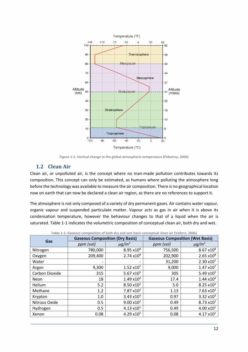
Earth's atmosphere is host to the air we breathe, barring its escape into space. It is occupied by four
primary layers, namely the troposphere, stratosphere, mesosphere and thermosphere, in ascending
order as seen in Figure 1-1. There are significant changes in the properties of air between these layers,
due to changes in temperature and pressure. These changes can be simply explained by the ideal gas
law in equation 1-1 (Clapeyron, 1834).
𝑝𝑉 = 𝑛𝑅𝑇 ( 1-1 )
1.1.1 Thermosphere
The thermosphere is the highest layer in the atmosphere before reaching the exosphere, extending
from an altitude of approximately 80 km, however there is a significant continual variation in altitude
due to solar activity (Duxbury & Sverdrup, 2002). The temperature in this layer can exceed 1,200 °C,
however this would not be able to be transferred as sensible heat due to thermal radiation losses.
Water molecules are far too large and heavy to exist at this altitude, rendering the thermosphere free
of water vapour. Even air is scarce; so much so, that a single molecule can travel an average of one
kilometre before colliding with another (Donald, 2005). The International Space Station orbits within
the thermosphere at a mean altitude of 330 km, and a maximum altitude of 420 km (Peat, 2013).

11
1.1.2 Mesosphere
The mesosphere is the second highest layer of the atmosphere and occupies the volume between an
altitude of approximately 50 and 80 kilometres. Temperatures here decrease significantly as the
mesopause is approached, averaging -85 °C and reaching -186 °C, earning it's title as the coldest place
on earth (McNaught & Wilkinson, 1997).
Conventional aircraft cannot operate at this altitude due to insufficient oxygen, and the atmospheric
drag and gravitation force is too great for orbital spacecraft; it can only be accessed by sounding
rockets and weather balloons. As a result, this layer in the atmosphere is poorly understood.
1.1.3 Stratosphere
The stratosphere is the third highest layer in the atmosphere, ranging between an altitude of
approximately 12 and 50 kilometres, and host to the ozone layer. The temperatures in the upper,
tropopause, and lower, stratopause, layers of the stratosphere range between -60 °C and 0 °C
respectively; inversely proportional to the decrease in altitude (James ,1993). This is due to the ability
of the ozone layer to absorb UV radiation from the sun.
Atmospheric conditions in the stratosphere are very stable, due to the temperature profile. This allows
specialised aircraft to access this altitude, and maintain optimized fuel burning efficiencies and low
drag-force losses.
1.1.4 Troposphere
The troposphere extends from the earth's surface towards the tropopause, thus being the lowest layer
of the atmosphere. Temperatures range between -60 °C and 15 °C and the atmospheric pressure is
sufficient to sustain the majority of life-forms and activity. It is composed of a variety of gasses,
primarily nitrogen and oxygen; other trace gasses are present in small concentrations.
The troposphere is the atmospheric layer in which the industry operates, thus it will be the primary
focus of this study.
12
Figure 1-1: Vertical change in the global atmospheric temperature (Pidwirny, 2006)
1.2 Clean Air Clean air, or unpolluted air, is the concept where no man-made pollution contributes towards its
composition. This concept can only be estimated, as humans where polluting the atmosphere long
before the technology was available to measure the air composition. There is no geographical location
now on earth that can now be declared a clean air region, as there are no references to support it.
The atmosphere is not only composed of a variety of dry permanent gases. Air contains water vapour,
organic vapour and suspended particulate matter. Vapour acts as gas in air when it is above its
condensation temperature, however the behaviour changes to that of a liquid when the air is
saturated. Table 1-1 indicates the volumetric composition of conceptual clean air, both dry and wet.
Table 1-1: Gaseous composition of both dry and wet basis conceptual clean air (Vallero, 2006)
Gas Gaseous Composition (Dry Basis) Gaseous Composition (Wet Basis)
ppm (vol) μg/m3 ppm (vol) μg/m3
Nitrogen 780,000 8.95 x10⁸ 756,500 8.67 x10⁸
Oxygen 209,400 2.74 x10⁸ 202,900 2.65 x10⁸
Water - - 31,200 2.30 x10⁷
Argon 9,300 1.52 x10⁷ 9,000 1.47 x10⁷
Carbon Dioxide 315 5.67 x10⁵ 305 5.49 x10⁵
Neon 18 1.49 x10⁴ 17.4 1.44 x10⁴
Helium 5.2 8.50 x10² 5.0 8.25 x10²
Methane 1.2 7.87 x10² 1.13 7.63 x10²
Krypton 1.0 3.43 x10³ 0.97 3.32 x10³
Nitrous Oxide 0.5 9.00 x10² 0.49 8.73 x10²
Hydrogen 0.5 4.13 x101 0.49 4.00 x101
Xenon 0.08 4.29 x10² 0.08 4.17 x10²

13
The values in the table 1-1 are expressed as metric units, which is micro grams per cubic meter of air.
A simple calculation is used to convert the values in ppm (parts per million) to μg/m3, indicated in
equation 1-2. For this calculation, a standard temperature and pressure are assumed as 25°C and
101.325 kPa respectively.
1 ppm = 1 liter pollutant
106 liter air
= (1 liter/22.4) × MM × 106𝜇𝑔/𝑔𝑚
106 liters × 298𝐾/273𝐾 × 10−3𝑚3/𝑙𝑖𝑡𝑒𝑟
( 1-2 )
= 40.9 × MM 𝜇𝑔/𝑚3
1.3 Particulate Matter Particulate is the collective term for small solid particles and droplets of liquid; it originates from both
man-made and natural sources. The produced particulate is indicated in table 1-2, and it is interesting
to note that natural sources generate a larger sum total of particulate than man-made sources;
however the man-made particulate pollution quantity is far from negligible (Weiner & Matthews,
2003).
The values in table 1-1 does not incorporate the particulate matter that is always present in air, varying
in weighted presence depending on various factors. Each gas and vapour exists as an individual
molecule, and its movement is random. Particles form as a result of molecules that join together; both
similar and dissimilar. The behaviour of these particles depends on the conditions of the atmosphere,
as they can serve as a surface for vapours to condense to, or a chemical reaction can take place
between the molecules and the atmosphere.
It is common for particles to adhere to each other when they collide in the atmosphere, due to the
attractive forces on their surfaces. The agglomeration of the particles becomes progressively larger,
and thus increases in mass. The particles eventually falls from the air, as its mass is too great to remain
airborne; the process is known as sedimentation (Boubel, et. al., 1994). The presence of a particle in
the air is dependent on its weight versus its aerodynamic diameter and displacement of atmospheric
volume. The mass of a particle can be expressed using equation 1-3, where the mass (mp), density (ρ)
and radius (r) are in metric units.
𝑚𝑝 =
3
4𝜋𝜌𝑟3
( 1-3 )
Particulate matter originates from both natural and man-made sources. The annual discharge of
particulate matter from natural and man-made sources is 800 - 2,000 and 200 - 500 million tons
respectively (A Kumar De, A Kumar De, 2005).

14
Table 1-2: Annual world-wide discharge of particulate matter into the atmosphere (Kumar de and Kumar de, 2005)
Particulate Matter
Annual Discharge
Natural Sources Man-Made Sources
Million Tons Million Tons
Total Particles 800 - 2,000 200 - 450
Dust and Smoke - 10 - 90
Salt and Forest Fires 450 - 1,100 -
Sulphate 130 - 200 130 - 200
Nitrate 330 - 35 140 - 700
Hydrocarbons 15 - 20 75 - 200
Particulate varies in size from 0.0002μm to 500μm, depending on their composition and density. Clean
air can contain as little as a few hundred particles per cm³, however highly polluted urban and
industrial air can exceed 100,000 per cm³.
There is a greater presence of particulate matter in the troposphere due to the increased density and
gravity at lower elevations. The volume of atmosphere lower than 100m is highly polluted above urban
and industrial areas. The pollutants in the atmosphere undergo a chemical reaction in the presence of
water vapour, oxygen and UV radiation. These reactions produce secondary pollutants, as indicated
below, which are harmful to vegetation, animals, material and humans.
𝐶𝑂2 + 𝐻2𝑂 ⇌ 𝐻2𝐶𝑂3 Carbon dioxide → Carbonic acid
𝑆𝑂2 + 𝐻2𝑂 ⇌ 𝐻2𝑆𝑂3 Sulphur dioxide → Sulphurous acid
𝑁𝑂𝑋 + 𝐻2𝑂 ⇌ 𝐻𝑁𝑂3 Nitrogen oxides → Nitric acid
Meteorology is based on the physical properties of the atmosphere, such as temperature, pressure,
density, moisture and pollutants. Chemical reactions that take place in the atmosphere also have an
effect on these physical properties.
The dispersion of pollutants in the atmosphere is dependent on the movement of the air, which is set
in motion by temperature differences. This cycle dilutes the higher concentrations of pollution in area,
but transfers them to a different location as a result. Mankind is partly responsible for changes in the
earth's meteorology, by conducting activities as indicated in table 1-3.

15
Table 1-3: Major emission sources of pollutants (Spengler and Sexton, 1983)
Pollutant Major Emission Source
Allergens Animals, insects
Asbestos Fire retardant materials, insulation
Carbon dioxide Metabolic and combustion activities
Carbon monoxide Fuel burning, reduction and smelting processes
Formaldehyde Particleboard, insulation, furnishings
Micro-organisms Humans, fauna, flora, air-conditioners
Nitrogen dioxide Fuel burning
Organic substances Adhesives, solvents, building materials, volatilisation, paints
Ozone Photochemical reactions
Particles Re-suspension, combustion
Polycyclic aromatic hydrocarbons
Fuel combustion
Pollens Outdoor air, fauna
Radon Soil, building materials
Fungal spores Soil, fauna, internal surfaces
Sulphur dioxide Fuel combustion, calcining processes
1.4 Air Quality Standards Each pollutant has a TLV (Threshold Limit Value) which can be hazardous to our health if exceeded.
Typical pollutants in the industry are indicated in table 1-4 with each of their TLVs. Typically, a person
can be exposed to a pollutant, provided it is below the TLV, for no more than 40 hours per week
without having adverse health effects.
Table 1-4: Threshold Limit Values (TLV) for a variety of common gases and vapours in the industry (Kumar De and Kumar de, 2005)
Pollutant Threshold Limit Values
ppm mg/m3
Acetone 750 1780
Ammonia 25 18
Arsenic 0.2 - 0.5 -
Benzene 10 20
Cadmium - 0.05
Carbon dioxide 5000 9000
Carbon monoxide 50 50
Carbon tetrachloride 5 30
Chlorine 10 30
Chloroform 10 50
Hydrogen chloride 5 7
Hydrogen sulphide 10 14
Lead - 0.2
Nitric oxide 25 30
Ozone 0.1 0.2
Sulphur dioxide 2 5

16
Environmental Awareness Environmental awareness is on the increase all around the world, and environmental sustainability
has become a massive movement to preserve our planet earth, with which we have been blessed.
Activities have been derived to reduce the negative influence that mankind has on the environment,
and many of these activities have become a global standard by which to conform. These activities
range from pollution treatment plants, to the intervening of certain production processes which result
in pollution, to the redesigning of products and services to lower their environmental impact (Vezzoli
& Manzini, 2007).
To better understand the root causes of our environmental problems, a closer look needs to be taken
at mankind; more specifically Western civilization. Western civilizations are often described as
destructive, exploiting, and a general uncaring attitude towards the environment. Many arguments
exist regarding the origin of our destructive tendencies towards the environment, which include
religion, social structure, economic structure, and how we accept technology (Peirce et al., 1998).
No matter what the origin of our tendencies is, it is important to maintain an ethical attitude towards
the environment. The environment must be treated as an entity, because it is something that mankind
shares. By polluting an area through a production process or service, the direct environment is
affected which, in turn, affects the population, fauna and flora residing in that area. Ralph Waldo
Emerson expressed his thoughts on the instrumental value of nature to mankind as material wealth,
the potential to recreate, and aesthetic beauty. Environmental ethics can be considered as a
conservational ethic, because it involves conserving resources to benefit us in the long-term
(Saravanan, et al., 2005).
2.1 Global Emissions Figure 2-1 indicates the annual carbon emission contribution by region since the 1800’s. It is clear that
there is an exponential increase, which is influenced by the increase in technological processes, and
the growth in population.
Even though the industry (processes, mining and transportation) contributes the largest part towards
man-made pollution and emission, it is important to understand that each and every one of us has a
moral accountability and responsibility to preserve our environment. This is not only beneficial to
man-kind, but generations to follow.
Every positive contribution that a person makes, however small, ultimately makes a large positive
contribution towards environmental preservation on the whole. We must maintain the attitude that,
even though we are tiny in relation to a factory or mine, we are instrumental in setting a standard of
environmental conservation, and that this attitude needs to start small in our personal actions; it will
then filter through to the larger industries.

17
Figure 2-1: Linear scale of annual carbon emissions by region (Marland et al., 2007)
2.2 Environmental Legislation in South Africa Regulations of environmental protection in South Africa can be traced back to the 1940’s, which
indicates early awareness in terms of environmental conservation (Van der Linde & Feris, 2010).
Legislation, however, was only introduced much later as The Environmental Conservation Act, Act 73
of 1989. In September 1997 the Environmental Impact Assessment Regulations were promulgated.
This contributed towards a proactive approach to mitigate and manage negative environmental
impacts.
Section 24 (The Environmental Law) was included into the South African Constitution, Act 108 of 1996,
which entitles every person to an environment which is not detrimental to their health and well-being.
To make this constitutional mandate even more effective, the environmental law in South Africa has
been under intense revision since 1996. The National Environmental Management Act 107 of 1998
was promulgated to support and increase the effectiveness of this constitutional mandate (Van der
Linde & Feris, 2010). The National Environmental Management Act is a progressive development
which sets environmental standards to guide government, institutions and individuals in making
environmental decisions. The National Environmental Management Act also provides the following
elements:
Environmental principles
Co-operative governance
Duty of care
Enforcement mechanisms
Integrated environmental management
Additional environmental management acts have been promulgated, such as The National
Environmental Management: Waste Act of 2008, which strengthens The National Environmental
Management Act.

18
2.3 Offences and Penalties For the legislation to be effective, government has the right to enforce penalties on any entity that
does not abide by the rules and regulations set out by the relevant act.
2.3.1 Offences
Section 51 of the National Environmental Management: Air Quality Act 39 of 2004 stipulates the
possible offences regarding air quality. The following are important:
Provision needs to be made in terms of the following:
o Section 22: Licences and listing
o Section 25: Consequences of involvement of an appliance or action declared as a
controlled emitter
o Section 35(2): Responsibility for controlling and preventing offensive odour emissions
Pollution prevention plans need to be drafted and submitted, according to Section 29(1)b and
Section 29(2)
An atmospheric impact report needs to be submitted, according to Section 30
The Minister needs to be notified, according to Section 33
The standards for a controlled emitter, according to Section 24
2.3.2 Penalties
Section 52 of the National Environmental Management: Air Quality Act 39 of 2004 stipulates the
penalties which can be evoked on individual or institution if convicted of an offence referred to Section
51 above.
1) The following penalties can be evoked:
a) A maximum fine of R10 million and/or 10 years imprisonment for an initial offence
b) A maximum fine of R5 million and/or 5 years imprisonment as a second or subsequent
offence to the initial offence
2) When the fines are imposed, the following needs to be considered:
a) The severity of the offence in terms of safety, well-being, health and the environment
b) The benefits (whether monetary or other) that where accrued through the offence
c) The contribution towards the total pollution in that area
2.4 Industrial Pollution More than 90 per cent of air pollution around the world is comprised of five primary pollutant
contributors (Kumar De & Kumar De, 2001), and the primary contributor of the total pollutants
globally is transportation (46 per cent). The five pollutants are:
1) Particulates
2) Carbon dioxide (CO2)
3) Nitrogen oxides (NOX)
4) Hydrocarbons (HC)
5) Sulphur oxides (SOX)
Carbon monoxide is the largest pollutant in the industry, which has a total global emission mass of
more than all the other pollutants combined. Particulate pollutants, however, are much more
poisonous and dangerous than any of the other pollutants (Kumar De & Kumar De, 2001).

19
Table 2-1 indicates the air quality standards as defined in Schedule 2 of Section 63 of the National
Environmental Management: Air Quality Act 39 of 2004.
Table 2-1: Air quality standards according to Schedule 2 of Section 63 of the National Environmental Management: Air Quality Act 39 of 2004
Composition
Maximum Instant
Peak @ 25°C and
Atmospheric
Pressure
Maximum
Average Over 10
Minutes
Maximum Average
Over 1 Hour
Maximum Average
Over 24 Hours at a
Maximum of 3
Times per Year
Value Unit Value Unit Value Unit Value Unit
Ozone (O3)
0.25 ppm - 0.12 ppm -
Nitrogen Oxides (NOX)
1.4 ppm - 0.8 ppm 0.4 ppm
Nitrogen Dioxide
(NO2)
0.5 ppm - 0.2 ppm 0.1 ppm
Sulphur Dioxide (SO2)
500 μg/m3 0.191 ppm 0.048 ppm -
Lead (Pb) 2.5
μg/m3
monthly
average
- - -
Particulate Matter
<10μm (PM10) 60
μg/m3
annual
average
- - 180 μg/m3
Total Suspended
Solids 100
μg/m3
annual
average
- - 300 μg/m3

20
Pollution Control Air pollution control can generally be described as the technology of “separation” (Schifftner, 2002).
This means that pollutants are separated from the carrier gas. By separating the pollutants from the
carrier gas, the pollutants can then be easily collected and then disposed of, or recycled.
The problem with gaseous pollutants, especially aerosols which are fine solid or liquid particles usually
smaller than 0.5μ, is that we inhale them. Once inhaled, our respiratory systems are susceptible to
absorbing these gases. The toxicity is not always the problem; it’s that the pollutant attaches itself to
the bronchial area and alveoli sacs. The lungs then become lined with these pollutants, and the
absorption of oxygen is restricted; thus suffocation becomes the threat and not necessarily the
toxicity.
There are many solutions to pollution control in the industry, each of which has its own advantages
and disadvantages. There are many criteria to consider when selecting the appropriate pollution
control system.
3.1 Wet Collection Wet collectors make use of the viscosity of a liquid, usually water, to separate the pollutant from the
carrier gas. Studies conducted around the rate of particles settling and motion kinetics, have indicated
that particles larger than 5μm behave inertially, while particles smaller than 2μm behave like gases
(Schifftner, 2002).
Wet collectors or scrubbers make use of the following three principles for separation to occur,
illustrated in Figure 3-1:
Impaction
Impaction is the most recognisable method of particulate removal (Schifftner & Hesketh, 1986).
This occurs when the pollutant accelerates and is impacted into a droplet of liquid or a surface.
The kinetic energy and inertia is sufficient for the particle to follow a predetermined path, and
then penetrate the surface tension of the scrubbing liquid droplet. Once the particle has
penetrated and is inside the droplet, the combined aerodynamic diameter of the droplet and
particle is larger, which makes it easier to separate from the carrier gas.
Interception
Interception occurs in the particles which are not collected by impaction. Rather, they travel
close enough to the surface of the liquid droplet to be attracted; however the particle
penetrates the droplet at an angle far less than 90° (Schifftner & Hesketh, 1986). The particle
does not have sufficient inertia to travel in a predicted path, yet it has enough kinetic energy to
penetrate the surface tension of the droplet.
Diffusion
Diffusion occurs mostly in particles smaller than 0.5μm. As discussed earlier, a particle smaller
than 2μm tends to behave like a gas; which incorporates electrostatic forces, turbulence factors
and gas density irregularities (Schifftner & Hesketh, 1986). The particle bounces between the
droplet and the gas stream which forms around the droplet. Once the particle has attached
itself to the surface of the droplet, there is insufficient energy for the particle to penetrate the
surface tension of the droplet. In impact plate is then used to force the particulate to be
engulfed by the droplet.

21
Figure 3-1: Three methods of particulate removal with a wet system (Schifftner, 2002)
3.1.1 Venturi Scrubbers
Venturi scrubbers are a type of wet scrubber that makes use of a sudden change in the carrier gas
velocity to atomise streams of liquid into tiny droplets; depending on the application, the scrubbing
liquid is usually water (Schifftner, 2002). This sudden change in the carrier gas velocity is implemented
by creating a pressure drop across the venturi throat, which results in the acceleration of the gas
(Theodore, 2008). Particulate matter and soluble gasses are then transferred into the water droplets.
Venturi scrubbers are able to remove particulate with an aerodynamic diameter as small as 0.6 μm.
Studies have also been conducted where sub-micron particles have been removed when a pressure
drop of about 15kPa was induced in the venturi (Schifftner, 2002). Venturi scrubbers are also capable
of handling large volumetric flow rates of carrier gas, whilst still maintaining the desired efficiency.
3.1.2 Packed Towers
Packed towers work similarly in principal to a venturi scrubber, however it consumes less energy to
atomise a liquid. A packed tower is a hollow column that contains a fill, such as pall-rings, which
increases the surface area of the tower. Liquid then enters the top of the column, and the gas stream
enters at the bottom. The column is always wider than the inlet duct, which allows the upward velocity
of the gas stream to decrease. The upward velocity of the gas stream is determined as a function of
the contact time required between the liquid and the gas.
Packed towers are commonly used for the treatment of noxious gas streams, and the neutralization
of acidic gas streams. The dosing agent is added to the recirculation liquid, thus being dispersed across
the whole area of the tower.

22
Figure 3-2: Packed tower scrubber (Schnelle & Brown, 2000)
3.1.3 Fluidized Bed Scrubbers
Fluidized bed scrubbers make use of a two-phase mixture of gas and liquid, similar to the operating
principal of a fluidized bed boiler. The mixture is a constantly agitated bed, into which the gas is
injected. The agitation is designed to increase the mass transfer rate, as the dissolution of a gas into
liquid is improved by stirring (Schifftner, 2002).
These scrubbers are primarily used in gaseous applications where the particulate present can cause
blockages in other designs, such as packed towers. The particulate is generally in the carrier gas
stream, however it can be a by-product of the absorption reaction. Typical applications include
Chlorine (Cl2) and chlorine dioxide (ClO2) control
Sulphur dioxide (SO2) control using caustic (NaOH) as a neutraliser
Sulphur dioxide (SO2) control using a limestone slurry
Odour control like hydrogen sulphide (H2S)
Gas quenching and condensing
Pre-scrubbing of gases upstream of high efficiency elimination devices
3.2 Dry Collection For large particulate matter which exceeds an aerodynamic diameter of about 50μm, the most
common collectors are knock-out chambers and traps (Schifftner, 2002). The principle is to slow down
the particle as far as possible so that the particle will drop out.
3.2.1 Filtration Collector
Collection devices that make use of fabric bags to filter out particulate matter are usually referred to
as “baghouses” (Schnelle & Brown, 2000). These bags are mounted on a tube sheet, which is arranged

23
closely together and enclosed in a large housing. These types of filters are typically used when the
particulate matter size ranges between 50μm and 75μm.
Baghouses separate the contaminant from the carrier gas by passing the gas through a filtration media
(Schnelle & Brown, 2000). The filtration media is usually made of one of the following:
Fabric (such as industrial cloth)
Porous material (such as ceramic candles or tubes)
Paper (such as the bags inside household vacuum cleaners)
Each of these different filtration media types are used for a specific application, typically depending
on the following aspects of the application:
Contaminant type and composition
Contaminant size (aerodynamic diameter)
Volumetric flow rate of the carrier gas
Inlet temperature of the carrier gas
Inlet pressure of the carrier gas
The inlet temperature of the carrier gas is very important to consider, because the filtration media can
be damaged if the temperature is too high; usually exceeding 260 °C (Schnelle & Brown, 2000). When
applications exceed these temperatures, evaporative coolers are used to reduce the carrier gas
temperature. This, however, warrants larger construction, cost, ground area, operating power
consumption, and maintenance implications.
Figure 3-3 : Typical fabric filter (Schnelle & Brown, 2000)
3.2.2 Dry Cyclone Collector
Another form of a dry collector is a dry cyclone collector, which makes use of the angular velocity and
centrifugal force of the particulate to force them outward onto the inner surface of the cyclone shell.
The particulate then slides down the sides of the cyclone and is deposited through a hopper into a
collection container. The basic principal of a typical dry cyclone collector is indicated in Figure 3-2.

24
Figure 3-4 : Standard cyclone (Schnelle & Brown, 2000)
Schifftner (2002) states that a cyclonic collector’s means of particulate removal is based on Newton’s
second law (F = m∙a). The centrifugal force is given by
𝐹 =
𝑚𝑉2
𝑟 ( 3-1 )
Where the centrifugal force (F), mass of the particle (m), velocity of the particle (V) and the radius of
the cyclone (r) are applicable.
Due to the separation of the particles relying on the mass of the particles, as in equation 3-1, the
smaller the particle, the less mass it has and the more difficult it is to remove. Therefore, the efficiency
decreases as the particulate size of the pollutant decreases, as seen in Figure 5. This is known as
Lapple’s efficiency curve (Schnelle & Brown, 2000).
This efficiency is based on Lapple's efficiency correlation as indicated in equation 3-2 (Schnelle &
Brown, 2000).
𝜂𝑗 =
1
1 + (𝑑𝑝50
𝑑𝑝𝑗)
2 ( 3-2 )
3.2.3 Electrostatic Precipitators (ESP)
Dry ESP’s are typically used to remove the particulate from the following applications which emit flue-
gas exhaust gas (Schifftner, 2002):
Cement production kilns
Power station boilers
Paper production mills
Metal processing and production plants
25
Glass production furnace
Similar industrial applications
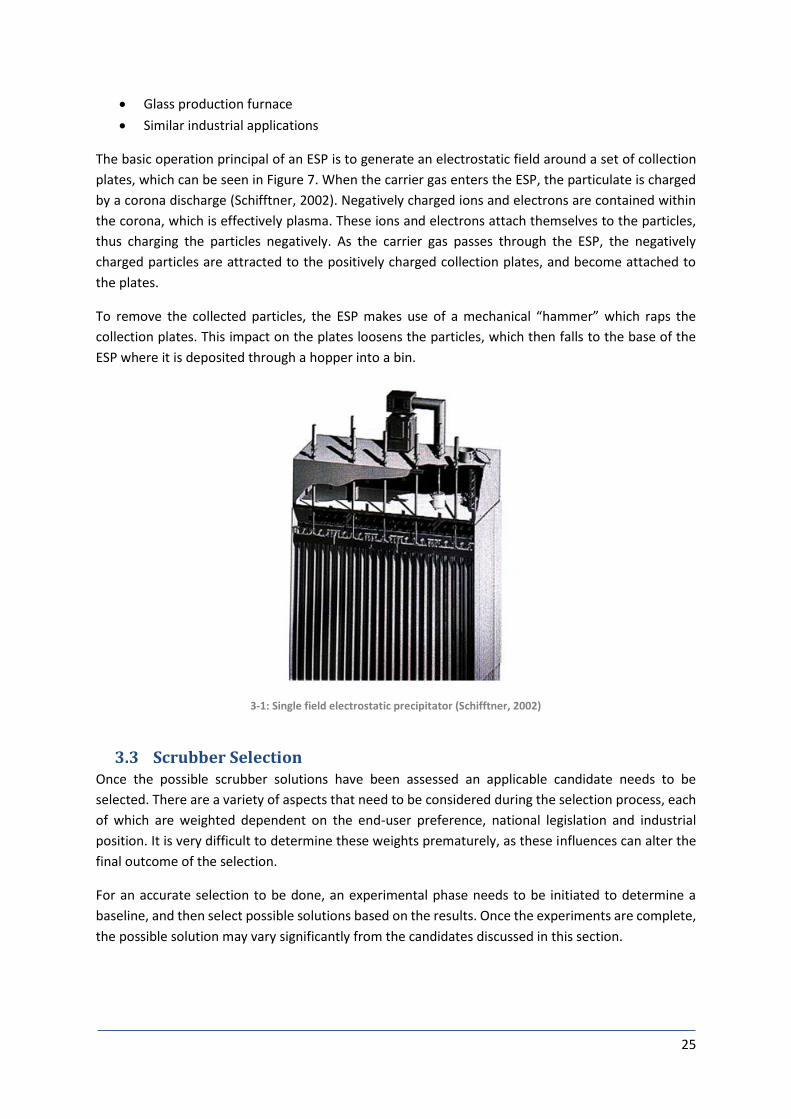
The basic operation principal of an ESP is to generate an electrostatic field around a set of collection
plates, which can be seen in Figure 7. When the carrier gas enters the ESP, the particulate is charged
by a corona discharge (Schifftner, 2002). Negatively charged ions and electrons are contained within
the corona, which is effectively plasma. These ions and electrons attach themselves to the particles,
thus charging the particles negatively. As the carrier gas passes through the ESP, the negatively
charged particles are attracted to the positively charged collection plates, and become attached to
the plates.
To remove the collected particles, the ESP makes use of a mechanical “hammer” which raps the
collection plates. This impact on the plates loosens the particles, which then falls to the base of the
ESP where it is deposited through a hopper into a bin.
3-1: Single field electrostatic precipitator (Schifftner, 2002)
3.3 Scrubber Selection Once the possible scrubber solutions have been assessed an applicable candidate needs to be
selected. There are a variety of aspects that need to be considered during the selection process, each
of which are weighted dependent on the end-user preference, national legislation and industrial
position. It is very difficult to determine these weights prematurely, as these influences can alter the
final outcome of the selection.
For an accurate selection to be done, an experimental phase needs to be initiated to determine a
baseline, and then select possible solutions based on the results. Once the experiments are complete,
the possible solution may vary significantly from the candidates discussed in this section.

26
Industrial Application An electric arc-furnace in the industry requires a primary off-gas scrubbing system to be designed and
implemented. The furnace characteristics are indicated in table 4-1.
Table 4-1: Physical characteristics of the furnace
Furnace Physical Characteristics
Description Type
Furnace Type Enclosed submerged arc furnace
Process Type Reduction process
Products Ferromanganese
Furnace Load 42MW, 65 MW maximum
Transformer Rating 81 MVA
Reductant 60% Ore, 40% Coke
Operation Continuous (24 hours per day, 365 days per year)
The furnace is enclosed to prevent the escape of gases from the process. A sealed system is critical to
contain thermal energy for process optimization, as well as being a legal requirement concerning
emission laws. Being a submerged arc process, the ore and reductant are mixed before charging the
furnace. The electrodes are submerged in the charge material, and the new cold-charge forms a layer
on top of the molten bed, which contributes towards the containment of thermal energy.
Table 4-2: Assumed furnace off-gas properties
Off-Gas Properties Average Maximum Minimum
Value Unit Value Unit Value Unit
Volume 23 524 Nm³/hr 40 000 Nm³/hr 0 Nm³/hr
Temperature 550 °C 900 °C Ambient -
Inlet Dust Loading 50 g/Nm³ 150 g/Nm³ 20 g/Nm³
Particle Size Distribution 30 μm 300 μm 0.3 μm
Required Outlet Emissions - - <30 mg/Nm³ - -
The off-gas properties of the furnace process are assumed, and therefore need to be verified through
experimentation. The furnace is assumed to yield an average of 23,524 Nm3/hr with a dust load of
approximately 50 g/Nm3, as indicated in table 4-2.
Table 4-3: Assumed primary off-gas composition
Furnace Primary Off-gas Composition
Composition Target Range
Carbon monoxide (CO) 60.0 % 50.0 – 70.0 %
Carbon dioxide (CO2) 16.0 % 10.0 – 25.0 %
Oxygen (O2) 0.5 % 0.0 – 2.0 %
Hydrogen (H2) 10.0 % 4.0 – 25.0 %
Methane (CH4) 1.2 % 0.5 – 4.0 %
Nitrogen (N2) 9.6 % Balance

27
The off-gas composition of the furnace process is assumed, and needs to be verified though
experimentation. Each gas within the composition fluctuates during the reduction process, as
indicated in table 4-3, and therefore an average needs to be determined for design purposes.
4.1 Process Overview This study will focus primarily on cleaning the primary off-gas of a ferromanganese electric arc furnace
in the industry. Therefore, the environmental impact concerned will be that of air quality. This poses
a complex analysis of a significant amount of data and information involved in this unique field of
study; the outcome, however, will be directly beneficial towards the environment, which ultimately
benefits mankind.
The design of a gas cleaning system for any application requires an in-depth knowledge of the process
involved before and after the cleaning of the gas. There are similarities between gas cleaning systems
in different applications which can be considered constants. This study, however, will assess the
process before, during and after the gas cleaning system so that each stage of the process can be fully
understood. This knowledge can then be applied to design a gas cleaning system in an application
different to that of this study.
The complete cycle of the gas is indicated in Figure 4-1 below, which is the basis of this study. Each
stage will be researched and discussed in detail, which will then lead to a detailed design of a gas
cleaning system for the application.
INDUSTRIAL
APPLICATION
RAW GAS
GAS CLEANING
SYSTEM
ENVIRONMENT
CLEAN GAS
Figure 4-1: Gas cycle of an industrial application process
The gas cycle gas can be broken down into three stages:
1. Application - refers to the process that generates the raw gas.
2. Gas cleaning system - process that cleans the raw gas by removing particulate
3. Environment - space that the gas occupies after being discharged
Due to the nature of this study, the most relevant legislation is The Air Quality Act. This act is formally
called National Environmental Management: Air Quality Act 39 of 2004.

28
The act defines air pollution as the change in composition of air which contains smoke, soot, dust
including fly-ash, cinders or any type of solid particles, gases, fumes, aerosols and odorous substances.
4.2 Basic Furnace Operation It is important to understand the basic operation of a furnace, so that the requirements for the primary
off-gas cleaning system can be correctly interpreted. Figure 4-1 depicts the basic gas cycle for the usual
application and process, however the cycle must now be detailed for a better understanding of the
overall process from start to finish.
Once the overall process and application is understood, literature can then be applied as to what type
of cleaning system must be selected. This is the start of the primary off-gas cleaning system design,
because the correct selection of gas cleaning system is the first step in research for the solution to the
client requirements and specifications.
Figure 4-2 indicates a more detailed gas cycle process in the ferromanganese electric arc-furnace, with
detailed descriptions to follow.
INDUSTRIAL
APPLICATION
ENVIRONMENT
SECONDARY
OFF-GAS SCRUBBING
SYSTEM
METAL SLAG
CLEAN GAS
SECONDARY
OFF-GAS
PRIMARY OFF-GAS
SCRUBBING SYSTEM
PRIMARY
OFF-GAS
CHARGED
MATERIAL
Figure 4-2: Detailed gas cycle of a ferromanganese electric arc-furnace
Each component in Figure 4-2 needs to be considered when designing a new system, regardless of
how minor its impact. The tiniest component can often govern an outcome, which requires diligent

29
design and consideration. Each of the following components are critical during the evaluation stage of
a system, and need to be fully comprehended before proceeding:
Charged material - This is the absolute start of the process. The charged comprises of a mixture of
ore and reductant, which is distributed evenly into the furnace. The furnace electrodes are always
submerged, close to the furnace floor. An electric current is induced through the electrodes into
the charged material, which sustains the reduction process. Inside the furnace there are three
relevant components:
Cold reductant, at the top of the furnace, which has not yet started to reduce
Hot reductant, at the bottom of the furnace, which consists of both slag and metal. The slag
is less dense, and thus separates at moves upwards from the denser metal.
Off-gas which is generated by the process
Furnace - This is the vessel in which the smelting process takes place. The interior of the furnace is
lined with thick refractories, which protect the outer steel shell from the immense heat generated
during the process.
Primary off-gas - The primary off-gas is a by-product of the process over and above the metal and
slag. The composition of this gas is indicated in table 4-3, and particulate matter is also present in
the gas.
Primary off-gas scrubbing system - This is the system which cleans the gas, by removing a
predetermined percentage or mass of particulate matter. The client specifications in table 4-3
indicate that a maximum of 30 mg/Nm³ is allowed to be emitted into the atmosphere. This is the
primary focus of this study.
Metal and slag - The tapping takes place once the charged material has been reduced. Due to the
metal being at the bottom it is tapped first; either into a casting pot or casting bay, where it is
processed further. Once all the metal has been tapped from the furnace, the layer of slag moves
downwards to replace the void where the metal resided. The slag is then tapped from the furnace
on the opposite side from where the metal is tapped; also into a slag pot or slag bay.
Secondary off-gas - Due to the extreme heat of the metal and slag, there is a lot of energy within
these products. When they are tapped, the total surface area of the metal or slag increases, allowing
the energy to be released in the form of dust and particulate matter.

30
Secondary off-gas scrubbing system - The fumes and dust released during tapping also contributes
towards the total emissions of the furnace. Therefore, the secondary off-gas stream also needs to
be cleaned. This is not, however, the focus point of the study; the design criteria and client
requirements and specifications are very different to that of the primary off-gas scrubbing system.
Clean gas - This is the ultimate product of the gas cycle in this process. The clean gas which is
emitted, from both the primary and secondary off-gas cleaning systems, is measured to determine
the final particulate emission of the process. This data is then submitted in a report to the provincial
environmental department, as per Section 30 of the National Environmental Management: Air
Quality Act 39 of 2004.
Environment - The environment is ultimately what we strive to protect and preserve, as we have a
moral responsibility towards environmental conservation. Legislation and penalties should not be
the motivation for conforming to environmental conservation standards; the motivation should be
to preserve the earth which we have inherited. We only have one opportunity to prevent global
environmental disintegration.
4.3 Ferromanganese Smelting Process Before any attempt is made to initiate a concept design, it is important to understand the
ferromanganese smelting process, and evaluate it from first principals. By doing so, all assumptions
can be eliminated and a solution can be designed without compromising accuracy.
4.3.1 Background of the Smelting Process
When mined, the raw ingredient is a combination of iron-oxide and manganese-oxide. The presence
of these two molecules in the ore can be described as
𝐹𝑒2𝑂3 + 𝑀𝑛𝑂2
Due to the presence of oxygen molecules in both the iron- and manganese-oxides, it is a norm in the
industry to subject the ore to a high temperature in the presence of carbon, a reductant, known as a
reduction process. The reduction process reduces the iron- and manganese-oxides to
ferromanganese, and oxidises the elemental carbon. Insufficient oxygen atoms results in the carbon
undergoing partial oxidation and forming carbon monoxide which consists of two covalent bonds and
one dative covalent bond (Thompson, 2005). The mass balance in for this process is indicated in
equation 4-1.
𝐹𝑒2𝑂3 + 𝑀𝑛𝑂2 + 7𝐶 = 2𝐹𝑒𝑀𝑛 + 7𝐶𝑂 ( 4-1 )
When considering the production of ferromanganese in an electric arc furnace, a lot of attention needs
to be focused on the energy consumption which is dependent on the availability of oxygen in the ore,
and the reductant used. The Boudouard reaction is the primary focus when considering energy
consumption of the process, which is indicated in equation 4-2.

31
𝐶𝑂2 + 𝐶 = 2𝐶𝑂 ( 4-2 )
4.3.2 Ferromanganese Production
The most commonly produced manganese containing ferroalloy is high carbon (HC) ferromanganese,
which is produced either in a blast furnace or electric arc furnace (Tangstad & Olsen, 1995). Medium
carbon (MC) ferromanganese is produced by subjecting the HC ferromanganese to an oxygen stream
at high temperatures. This further oxidises the remaining carbon bound in the molten HC
ferromanganese, thus reducing the carbon content. MC ferromanganese is a higher grade than HC
and has increased costs to produce. Its production is therefore solely dependent on market prices.
Electric arc furnaces are more flexible than blast furnaces, as the slag can be further processed refined
ferromanganese. Reductant and electricity prices also dictate the type of process selected for the
reduction process.
4.3.3 Process Chemistry
A layout of a typical electric arc furnace is illustrated in Figure 4-2, indicating the molten bed of the
furnace, as well as the upper, cooler charge. The temperature in the cold charge layer ranges from
200 to 250°C. The charged material contains ore, reductant, flux in the form of carbonates,
limestone and quartzite.
ELECTRODES
COLD CHARGE
MOLTEN BED
Figure 4-3 : Section view of a closed electric arc furnace with the molten bed and cold charge layers
Evaporation of water takes place in the cold charge layer, which is considered in equation 4-3.
𝐻2𝑂(𝑙) = 𝐻2𝑂(𝑔) ∆𝐻2980 = 44 𝑘𝐽/𝑘𝑚𝑜𝑙
( 4-3 )
At temperatures below 700°C, a portion of the water vapour will react according to equation 4-4, as
there is always hydrogen present in the furnace off-gases.

32
𝐻2𝑂(𝑔) + 𝐶𝑂(𝑔) = 𝐻2(𝑔) + 𝐶𝑂2(𝑔) ∆𝐻2980 = −41.1 𝑘𝐽/𝑘𝑚𝑜𝑙
( 4-4 )
Another source of hydrogen is from Faraday's principle of electrolysis, which is the decomposition of
water into hydrogen and oxygen gas. The presence of massive electric current being passed through
the charge material is ideal for the reaction to take place, as indicated in equation 4-5. A third source
of hydrogen is the volatiles in the reductant.
2𝐻2𝑂(𝑙) → 2𝐻2(𝑔) + 𝑂2(𝑔) ∆𝐻2980 = −286 𝑘𝐽/𝑘𝑚𝑜𝑙
( 4-5 )
The carbonates which are added to the charge in the form of MgCO3 and CaCO3 start to decompose
at 400°C and 900°C respectively, and is indicated in equation 4-6 and 4-7.
𝑀𝑔𝐶𝑂3 = 𝑀𝑔𝑂 + 𝐶𝑂2(𝑔) ∆𝐻2980 = 101.1 𝑘𝐽/𝑘𝑚𝑜𝑙
( 4-6 )
𝐶𝑎𝐶𝑂3 = 𝐶𝑎𝑂 + 𝐶𝑂2(𝑔) ∆𝐻2980 = 178.3 𝑘𝐽/𝑘𝑚𝑜𝑙
( 4-7 )
The manganese ores contain alkali oxides, Na2O and K2O, which are reduced to metal vapour when in
the molten bed. These vapours then follow the gas stream to the cold charge layer where they oxidise
to form alkali carbonates, as indicated in equation 4-8.
2𝐾(𝑔) + 3𝐶𝑂(𝑔) = 𝐾2𝐶𝑂3(𝑙) + 2𝐶 ∆𝐻2980 = −1 010 𝑘𝐽/𝑘𝑚𝑜𝑙
( 4-8 )
As these alkalis circulate, heat is transferred from the molten bed to the cold charge layer, assisting
with pre-reduction and pre-heating of the charge material.
The reduction of manganese ores is a regenerative process, in that it is able to be reduced by both
carbon and carbon monoxide. The furnace effectively generates its own reductant once the smelting
process has reached a certain temperature.
Higher manganese oxides are dominant in manganese ores, which benefits the process from an energy
consumption approach. The higher oxides, MnO2, Mn2O3 and Mn3O4, can be easily reduced with CO,
as they are unstable compared to the lower oxides (Tangstad and Olsen, 1995). These reactions are
indicated in equations 4-9, 4-10 and 4-11.
𝑀𝑛𝑂2 +1
2𝐶𝑂 =
1
2𝑀𝑛2𝑂3 +
1
2𝐶𝑂2 ∆𝐻298
0 = −99.9 𝑘𝐽/𝑘𝑚𝑜𝑙 ( 4-9 )
1
2𝑀𝑛2𝑂3 +
1
6𝐶𝑂 =
1
3𝑀𝑛3𝑂4 +
1
6𝐶𝑂2 ∆𝐻298
0 = −31.3 𝑘𝐽/𝑘𝑚𝑜𝑙 ( 4-10 )
1
3𝑀𝑛3𝑂4 +
1
3𝐶𝑂 = 𝑀𝑛𝑂 +
1
3𝐶𝑂2 ∆𝐻298
0 = −16.9 𝑘𝐽/𝑘𝑚𝑜𝑙 ( 4-11 )
The reduction of higher oxide manganese is an exothermic reaction, producing a significant amount
of heat. This also contributes to the pre-reduction and pre-heating of the charge materials.
Once the furnace temperature has increased to 1000°C, the reaction that takes place on the reductant
surface is rapid enough to allow both the ore reduction (4-11) and the Boudouard reaction (4-12) to
react simultaneously.
1
3𝑀𝑛3𝑂4 +
1
3𝐶𝑂 = 𝑀𝑛𝑂 +
1
3𝐶𝑂2
∆𝐻2980 = −16.9 𝑘𝐽/
𝑘𝑚𝑜𝑙 ( 4-11 )

33
1
3𝐶 +
1
3𝐶𝑂2 =
2
3𝐶𝑂
∆𝐻2980 = +57.5 𝑘𝐽/
𝑘𝑚𝑜𝑙 ( 4-12 )
1
3𝑀𝑛3𝑂4 +
1
3𝐶 = 𝑀𝑛𝑂 +
1
3𝐶𝑂
∆𝐻2980 = +40.5 𝑘𝐽/
𝑘𝑚𝑜𝑙 ( 4-13 )
Due to the presence of iron in the manganese ore, the reduction of the iron oxides reacts concurrently
with the manganese oxide reduction. The following reactions take place:
1
3𝐹𝑒3𝑂4 +
4
3𝐶𝑂 = 𝐹𝑒 +
4
3𝐶𝑂2 ∆𝐻298
0 = −4.5 𝑘𝐽/𝑘𝑚𝑜𝑙 ( 4-14 )
1
3𝐹𝑒3𝑂4 +
4
3𝐶 = 𝐹𝑒 +
4
3𝐶𝑂 ∆𝐻298
0 = +225.4 𝑘𝐽/𝑘𝑚𝑜𝑙 ( 4-15 )
𝑀𝑛𝑂(𝑙) + 𝐶 = 𝑀𝑛(𝑙) + 𝐶𝑂(𝑔) ∆𝐻2980 = +246.8 𝑘𝐽/𝑘𝑚𝑜𝑙
( 4-16 )
𝑆𝑖𝑂2(𝑙) + 2𝐶 = 𝑆𝑖(𝑙) + 2𝐶𝑂(𝑔) ∆𝐻2980 = −286 𝑘𝐽/𝑘𝑚𝑜𝑙
( 4-17 )
𝐾2𝐶𝑂3(𝑙) + 2𝐶 = 2𝐾(𝑔) + 3𝐶𝑂(𝑔) ∆𝐻2980 = −286 𝑘𝐽/𝑘𝑚𝑜𝑙
( 4-18 )
Four zones can be described when considering the ore reduction process, which is indicated in Figure
4-3. These zones are temperature dependant and induce different reactions and mass balances, which
are as follows:
Zone 1: Drying and calcination Reduction at low temperatures, MnO2 → Mn2O3
Zone 2: Gas reduction Reduction of manganese-oxide, Mn2O3 → Mn3O4 and partial MnO
Zone 3: Direct reduction Reduction of iron-oxide, Fe3O4 → Fe
Zone 4: Smelting reduction Partial reduction of MnO to liquid metal

34
Charge in: 200°C
25°C ↓
↑
13.4CO
12.57CO2
Zone 1
9.5MnO2 + 4.7CO = 4.7Mn2O3 + 4.7CO2
11H2O(l) = 11H2O(g)
1.5H2O + 1.5CO = 1.5H2 + 1.5CO2
1.4MgCO3 = 1.4MgO + 1.4CO2
420°C ↓
↑
900°C
19.6CO
Zone 2
4.7Mn2O3 + 1.6CO = 3.2Mn3O4 + 1.6CO2
3.4Mn3O4 + 3.4CO = 10.2MnO + 3.4CO2
5CO2
653°C ↓
↑
1050°C
24.6CO
Zone 3
8C + 8CO2 = 16CO
2.5Mn3O4 + 2.5CO = 7.4MnO + 2.5CO2
0.8Fe3O4 + 3.3CO = 2.5Fe + 3.3CO2
773 kWh
1250°C ↓
↑
1420°C
14.41CO
Zone 4
14.4MnO + 14.4C = 14.4Mn + 14.4CO
0.014SiO2 + 0.028C = 0.014Si + 0.028CO
C = C
1401 kWh
1420°C ↓
Charge in Off-gas (dry) Slag Metal
MnOx (x = 1.7)
17.57 kmol Mn
Dolomitic limestone
10% H2O
339 kg C
5% H2
49% CO
46% CO2
33% MnO
11% Al2O3
18% CaO
26.8% SiO2
8% MgO
2.3% K2O
Balance ≈ 2%
79% Mn
14% Fe
7% C
0.04% Si
Figure 4-4 : Staged heat belance and material balance for a ferromanganese reduction process (Tangstad and Olsen, 2005)
In a scenario where the production of one ton of HC FeMn is required, the raw materials are combined
with compositions as in Figure 4-3 to produce the metal, slag and off-gas. The molten metal and slag
has a temperature of 1420°C; therefore the off-gas generated has the same temperature. The off-gas
enters zone 1 with an assumed temperature of 900°C, which is ideal for drying the cold charge and
decomposing the MgCO3 (Tangstad and Olsen, 2005).

35
It is a near impossible calculation to determine the exact off-gas temperature above the cold charge
in a furnace at any given time. This varies with the depth of the cold charge, the size of the charge
material, the heat transfer coefficient of the ore which is composition dependent, and the stability of
the reduction process. Eruptions within the furnace can cause the off-gas temperature to spike
instantly, exceeding 1000°C. An assumption can be made that the maximum and minimum off-gas
temperatures are 900°C and 200°C respectively, resulting in an average of 550°C, which will be used
to initiate the off-gas calculations. This value will, however, require experimental confirmation to
ensure that the most accurate value is used as a design base.
The ratio of CO2 to CO + CO2 is a function of the carbon consumed by the reduction process. It is
favourable towards the reduction process for a greater presence of CO, as described in equation 4-11,
however the yield of CO is dependent on the energy input into the furnace, as illustrated in Figure 4-
5. The energy consumption is a direct cost for ferromanganese production and there exists a trade-off
between energy input and CO reduction energy saving, however they are ultimately governed by the
carbon consumption, which is also a direct cost of production.
2 400
2 300
2 200
2 100
2 000
1 900
1 800
1 700
100 %
90 %
85 %
70 %
60 %
50 %
40 %
30 %
20 %
10 %
0 %
240 260 280 300 320 340 360 380 400
kW
h
CO
/(C
O +
CO
)2
2
kg C
CO /(CO + CO)22kWh
Figure 4-5 : Energy consumption vs. carbon consumption vs. the ratio of CO2 to total off-gas (Tangstad and Olsen, 2005)

36
Pre-Design Experimentation To initiate a preliminary design it is important to have values that are as accurate as possible to
minimise errors, which can result in an inefficient or unsuitable solution for the application. It is
commonplace in the industry for a client to conduct experiments before approaching consultants for
an engineered solution, so that a baseline can be established. This saves both time and money when
engineering a solution, however the following occurrences are most common:
Inaccurate experimental results due to:
o Incorrect sampling techniques
o Inaccurate calibration of sampling equipment
o Inadequate steps taken to preserve physical samples
o Incorrect testing methods applied at the laboratory
Unstable furnace conditions during sampling resulting in inconclusive results
Changes in furnace operating parameters during sampling, such as a change in the charge
material smelting recipe
Incorrect standards used for conducting experiments
It is critical to establish a reliable set of standards and experimenting criteria beforehand, so as to
eliminate inconsistencies and conclude a reliable baseline.
5.1 Critical Data There is an immense amount of information that can be collected from any process. The first step in
initiating the experimentation is to identify which information in relevant, and conduct the applicable
experiments. Experimentation is costly and timeous; it is wise to collect the least amount of data
necessary, without compromising accuracy and quality. Table 5-1 indicates typical data that is
necessary to design a gas scrubbing system, along with a motivation as to why it is relevant.
Table 5-1: Necessary data required for designing a scrubber system
Input Component Relevance
Gas temperature Type of cooling system is dependent on the inlet gas temperature
Governs material selection for the components
Critical for calculating an accurate actual gas flow rate
Gas pressure Governs material selection for the components
Critical for calculating an accurate actual gas flow rate
Gas composition Heat transfer is a function of each present gas
Type of neutralising system is dependent on the gas composition
Critical for stoichiometric calculations
Necessary for safe operating procedures to be generated
Particulate in the
gas stream
Type of scrubbing system is dependent on the particle size distribution
Scrubber efficiency is a function of the particle size distribution
5.2 Sampling Each component requires a specialized method of sampling to achieve accurate results. These
components can have adverse effects on the environment, which has forced legislation to strictly

37
monitor the sampling methods and maintain a standard to ensure consistency, i.e. two different
instruments sample under the same conditions and return results within an allowable tolerance.
5.2.1 Gas Temperature
5.2.1.1 Sampling Method
For a reliable data series, the furnace off-gas temperature needs to be monitored continuously over a
period of time at full power load. This will give an accurate representation of a mean temperature
value, as well as temperature spikes as a result in unstable smelting conditions.
The intense heat within the furnace demands a sampling instrument capable of high operating
temperatures, typically a high grade thermocouple. A Type-K thermocouple is capable of operating in
temperatures exceeding 1000C, which is in excess of the off-gas leaving Zone 2 as indicated in Figure
4-4.
The location of the instrument is critical for reliable data collection. When the furnace is charged, the
material is not always distributed evenly, which causes the height of the cold charged material in the
furnace relative to the bed varies. When the off-gas passes through a larger material height, more
heat is transferred, cooling the gas further. The opposite is true when the gas passes through less
height of material. To account for these possible differences, three thermocouples are used to sample
instead of one, as indicated in Figure 5-1. An average is then taken between the three thermocouples,
and this is used to determine a baseline for the standard operating temperature. The thermocouples
are located on the furnace roof, as this is the applicable gas temperature required for the scrubber.
Electrode
Thermocouple
Furnace Shell
Layout Lines
Figure 5-1: Layout of the thermocouples on the furnace roof relative to the electrodes

38
Data is collected for a period of 5 days at intervals of one hour to monitor the conditions in the furnace
as extensively as possible. During this period data during upset conditions is also collected, however
this does not occur often. These temperature spikes are still relevant as they must be taken into
account when selecting the construction material and to design for the necessary safety precautions
to protect the equipment.
5.2.1.2 Results
The results were conclusive, as indicated in table 5-2. The average gas thermal properties are
determined and used as the baseline for the design.
Table 5-2: Furnace temperature values
Furnace Temperature
Description Temperature
[C]
Average 310.50
Maximum 497.90
Minimum 244.00
Standard deviation 62.80
The values in table 5-2 are sufficient for the purpose of initiating design calculations. The data series
incorporates both a good average and visible minimum and maximum values. The average
temperature will be used to design for a constant operating temperature, whereas the minimum
values will be used to design safety features. There is a clear trend in Figure 5-2 of the furnace
temperature over time; this varies, as it is a highly reactive environment.
Figure 5-2: Furnace temperature over a period of five days
0.0
50.0
100.0
150.0
200.0
250.0
300.0
350.0
400.0
450.0
500.0
Tem
per
atu
re [C
]
Days
Furnace Temperature
0 1 2 3 4 5

39
5.2.2 Gas Pressure
5.2.2.1 Sampling Method
Furnace pressure is one of the most important control points on a furnace. Excessively low furnace
pressure results in a vacuum within the shell, inducing air ingress which can cause an explosion if the
correct stoichiometric ratio is achieved. Excessively high furnace pressure allows gas to escape to the
surrounding atmosphere, which then combusts and can damage the equipment in the surrounding
area. The pressure needs to be controlled very accurately and responsively to ensure safe operation
at all times. Furthermore, the gas pressure is used along with the gas temperature to determine the
density, which is critical when selecting gas displacing equipment (fans, compressors, etc.).
A differential pressure transmitter is used to continuously measure the internal furnace pressure over
a period of time. The transmitter measures the difference between the internal and atmospheric
pressure, as this is the relevant control parameter. Figure 5-3 indicates the configuration of the
transmitter.
1
2
39
5
6 7 8
4
Components
1 – Pressure transmitter2 – Atmospheric sampling inlet3 – Furnace sampling inlet4 – Moisture catch-pot5 – Auto drop-out valve6 – Furnace roof7 – Heat resistant seal8 – Take-off pipe9 – Maintenance shut-off valve
Figure 5-3: Pressure transmitter arrangement for the furnace internal pressure
5.2.2.2 Results
Upon completing the sampling, a relevant series of data was returned. The typical furnace pressure
values indicated in table 5-3. The maximum pressure indicated occurs when the gas yielded is greater
than the extraction capacity of the scrubber plant. The opposite is true for the minimum pressure,
which occurs when the gas extracted is greater than the furnace yield. Both cases are minimal when
considering the process, the leakage inward and outward is a function of the pressure difference, as

40
expressed in equation 5-1, where Aseal is the leak area on the furnace roof and p is the pressure
difference in Pa. The equation returns the result in m3/s.
𝑄𝑙𝑒𝑎𝑘 = 𝐴𝑠𝑒𝑎𝑙√
2𝑝
𝜌𝑔
( 5-1 )
Table 5-3: Furnace pressure values
Furnace Pressure
Description Pressure
[mmH2O]
Average 0.3
Maximum 6.2
Minimum -5.2
Standard deviation 3.3
There is a clear trend in Figure 5-4 of the furnace temperature over time.
Figure 5-4: Furnace pressure over a period of five days
5.2.3 Gas Composition
5.2.3.1 Sampling Method
Isokinetic sampling can be described as the extraction of a gas under normal operating conditions,
without altering external influences. Gas is subject to change when it undergoes a change in
temperature or pressure; therefore a sampling technique needs to be used in which both the
temperature and pressure are identical to the operational properties of the gas stream.
-6.0
-4.0
-2.0
0.0
2.0
4.0
6.0
8.0
Pre
ssu
re [
mm
H2
O]
Days
Furnace Pressure
0 1 2 3 4 5

41
There are many different standards for emission sampling including BS, EN and ISO. For this study the
Environmental Protection Agency (EPA) was used to sample the gas stream. There is a large variety of
properties that can be measured with a single isokinetic sample, including:
Temperature
Pressure
Mass flow rate
Particle size distribution
Particulate properties, i.e. density, composition
Gas composition
Volatile measurement
To measure all of these parameters, a reliable sampling system needs to be used in order to extract
the gas without changing any external effects. A typical sampling rig is indicated in Figure 5-5.
Figure 5-5: Isokinetic sampling rig (Environmental Protection Agency, 2000)
The probe is inserted into the gas stream and sealed off. Turbulence within the duct causes irregular
flow patterns which can affect the sampled result. According to the Environmental Protection Agency
(2000), the turbulence within the duct needs to be accounted for. There are two requirements
according to the EPA which need to be adhered to, namely:
Sampling needs to be conducted for at least one hour, or one normal cubic metre of gas needs
to be extracted

42
The sampling technique needs to account for the gas duct geometry
It is important to ensure that the equipment is calibrated, and that sampling is conducted is
accordance with the relevant standards. Figure 5-6 and 5-7 indicates the sections that a duct must be
divided into for accurate sampling of the gas stream.
0.316R
0.548R
0.707R
0.837R0.916R
R
Sample Point
Figure 5-6: Sampling points for a round duct

43
Sample Point
Figure 5-7: Sampling points for a rectangular duct
The sampling rig comprises of a number of different components, indicated in Figure 5-5. A
temperature sensor at the front of the probe is used to determine the gas density. A pitot tube
measures the dynamic velocity within the duct by applying Bernoulli’s law; the volumetric flow rate
can thus be determined.
The gas enters the gooseneck nozzle, which is parallel with the flow of gas, and then enters the heated
tube. This tube is connected to a fabric filter, which eliminates particulate with a diameter greater
than 0.3µm. Both the probe and the filter housing are heated so as to prevent premature
condensation of the gas.
Upon leaving the filter area, the gas enters a series of four impingers. These are mounted in an ice
bath to force the gas below its dew point. The first two impingers contain water, the third is empty
and the last silica gel. The first two impingers make use of the water for the gas to bubble through,
encouraging impingement in the water. The third impinger acts as a gravitation separator for the
majority of condensation. The last impinger contains a dehydrating agent to eliminate the last of the
moisture in the sampled gas stream. All four of these impingers are accurately weighed before the
sampling process starts, and then immediately afterwards.
A vacuum pump induces a draft in the rig at a fixed volumetric flow rate, which is measured by the
orifice at the pump exhaust. This reading is compared to the flow rate measured in the duct to
determine a scale. This is then extrapolated once the laboratory has verified the contents of the filter,
impingers and the gas composition.

44
5.2.3.2 Results
The gas composition results are indicated in table 5-4 by volume.
Table 5-4: Gas composition by volume
Gas Composition
Description Average Minimum Maximum
Carbon Monoxide 61.24 % 57.8 % 65.9 %
Carbon Dioxide 12.74 % 12.1 % 13.8 %
Hydrogen 9.77 % 8.60 % 11.8 %
Oxygen 1.10 % 0.20 % 1.80 %
Nitrogen 14.4 % 8.70 % 17.6 %
Methane 0.71 % 0.60 % 0.80 %
It is clear from table 5-4 that carbon monoxide is the predominant contributor towards the volumetric
composition percentage of the off-gas. CO forms in as partial oxidation in environments with
insufficient oxygen to generate carbon dioxide. The typical characteristics include
Colourless, odourless and tasteless
Harmful to humans when exposed to concentrations greater than 35 ppm
Flammable
5.2.4 Particulate Matter in the Gas Stream
5.2.4.1 Sampling Method
The range of particle sizes in the off-gas stream of a furnace is typically very large, which makes it
difficult to plot the range. A mathematical function can be used to determine the number frequency,
in the form of a log-normal distribution (Hinds, 1999) and is indicated in equation 5-2. The advantage
of this function is that it can cover a large range, and does not return negative values.
d𝑓 =
1
𝜎√2𝜋𝑒
−(𝑑𝑝−�̅�𝑝)2
2𝜎2 d𝑑𝑝
( 5-2 )
To sample the gas stream for particulate matter, the same isokinetic rig is used as described earlier,
however the tests in the laboratory are significantly different. A laser diffraction technique is used, in
which a laser pattern is passed through a particle to measure its geometrical dimension. This
technique is not a function of flow rate, i.e. it is not time based (De Boer, 2002).
The particulate was sampled at different furnace loads so as to determine the influence of power input
versus dust yield. The dust loading at the different power loads are indicated in table 5-5.
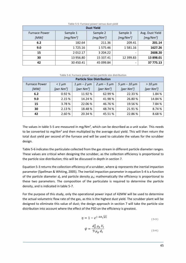
45
Table 5-5: Furnace power versus dust yield
Dust Yield
Furnace Power
[MW]
Sample 1
[mg/Nm3]
Sample 2
[mg/Nm3]
Sample 3
[mg/Nm3]
Avg. Dust Yield
[mg/Nm3]
6.2 182.64 211.36 209.41 201.14
9.0 1 725.16 1 575.46 1 581.16 1627.26
15 2 012.17 3 204.22 - 2608.20
30 13 956.80 15 337.41 12 399.83 13 898.01
42 30 450.41 45 099.84 - 37 775.13
Table 5-6: Furnace power versus particle size distribution
Particle Size Distribution
Furnace Power
[MW]
< 1 µm
[per Nm3]
1 µm – 2 µm
[per Nm3]
2 µm – 5 µm
[per Nm3]
5 µm – 10 µm
[per Nm3]
> 10 µm
[per Nm3]
6.2 0.92 % 11.92 % 62.99 % 22.33 % 1.84 %
9.0 2.15 % 14.24 % 41.98 % 26.80 % 14.84 %
15 3.78 % 22.06 % 46.76 % 19.56 % 7.84 %
30 2.13 % 18.48 % 48.74 % 21.91 % 8.74 %
42 2.60 % 20.34 % 45.51 % 22.86 % 8.68 %
The values in table 5-5 are measured in mg/Nm3, which can be described as a unit scalar. This needs
to be converted to mg/Am3 and then multiplied by the average dust yield. This will then return the
total dust yield per second of the furnace and will be used to calculate the values for the scrubber
design.
Table 5-6 indicates the particulate collected from the gas stream in different particle diameter ranges.
These values are critical when designing the scrubber, as the collection efficiency is proportional to
the particle size distribution; this will be discussed in depth in section 7.
Equation 5-3 returns the collection efficiency of a scrubber, where ψ represents the inertial impaction
parameter (Spellman & Whiting, 2005). The inertial impaction parameter in equation 5-4 is a function
of the particle diameter dp and particle density ρp; mathematically the efficiency is proportional to
these two parameters. The composition of the particulate is required to determine the particle
density, and is indicated in table 5-7.
For the purpose of this study, only the operational power input of 42MW will be used to determine
the actual volumetric flow rate of the gas, as this is the highest dust yield. The scrubber plant will be
designed to eliminate this value of dust; the design approach in section 7 will take the particle size
distribution into account where the effect of the PSD on the efficiency is greatest.
𝜂 = 1 − 𝑒(−𝑘𝑅√𝜓) ( 5-3 )
𝜓 = 𝑑𝑝
2 𝜌𝑝 𝑉𝑡
9 𝜇𝑔 𝑑𝑙
( 5-4 )

46
Table 5-7: Particulate composition
Particulate Composition
Element Percentage
[mass]
Density
[g/cm3]
Fe 0.8 % 7.874
Mn 30.5 % 7.210
S 28.2 % 2.070
C 40.5 % 1.900
Total 100.0 %
The gas yielded as a function of furnace power input was sampled, and is indicated in table 5-8.
Table 5-8: Gas yield as a function of furnace power input
Gas Yield
Furnace Power
[MW]
Gas Yield
[Am3/s]
Temperature
[C]
Gas Yield
[Nm3/s]
6.2 3.09 390.80 1.271
9.0 4.89 433.60 1.889
15 8.77 440.00 3.359
30 10.57 444.00 4.025
42 11.89 466.00 4.393
5.2.4.2 Dust Load Forecast
When a concept design is underway for a scrubber system, no all the furnace data is available. Usually
a furnace construction project entails all the services to build concurrently to ensure that production
can commence as early as possible. Therefore, a method was derived by using a curve-fitting tool in
Matlab to determine the relationship between furnace power input and dust yield. The plotted values
are indicated in Figure 5-8, and the yield rate is defined in equation 5-5.
𝑌 = 𝐴𝑒𝑘𝑃2.87
( 5-5 )
Where:
Furnace Power P is in MVA
Dust Yield Rate Y is in mg/s
Electrode Area Ae is in m2
Constant k is 0.02032

47
Figure 5-8: Dust yield rate versus furnace power input
Both constants in the equation are determined by the curve-fitting tool in Matlab. The total cross-
sectional area of the electrodes is governed by the furnace design, and is used in the equation as it is
the energy source over a surface that initiates the smelting process (Benilov, 2007).
5.2.5 Conclusion
All the pre-design experiments that were conducted returned results that were used to determine
conclusive trends and a reliable basis for the design to be initiated. When considering both
environmental and financial implications as a result of non-compliance, it is critical that the scrubber
system can operate at the required efficiency during conditions that cannot be forecasted. Therefore
the values used in the design phase are all based on the mean values during testing, however the
system must be designed to withstand operational peaks for short periods of time.
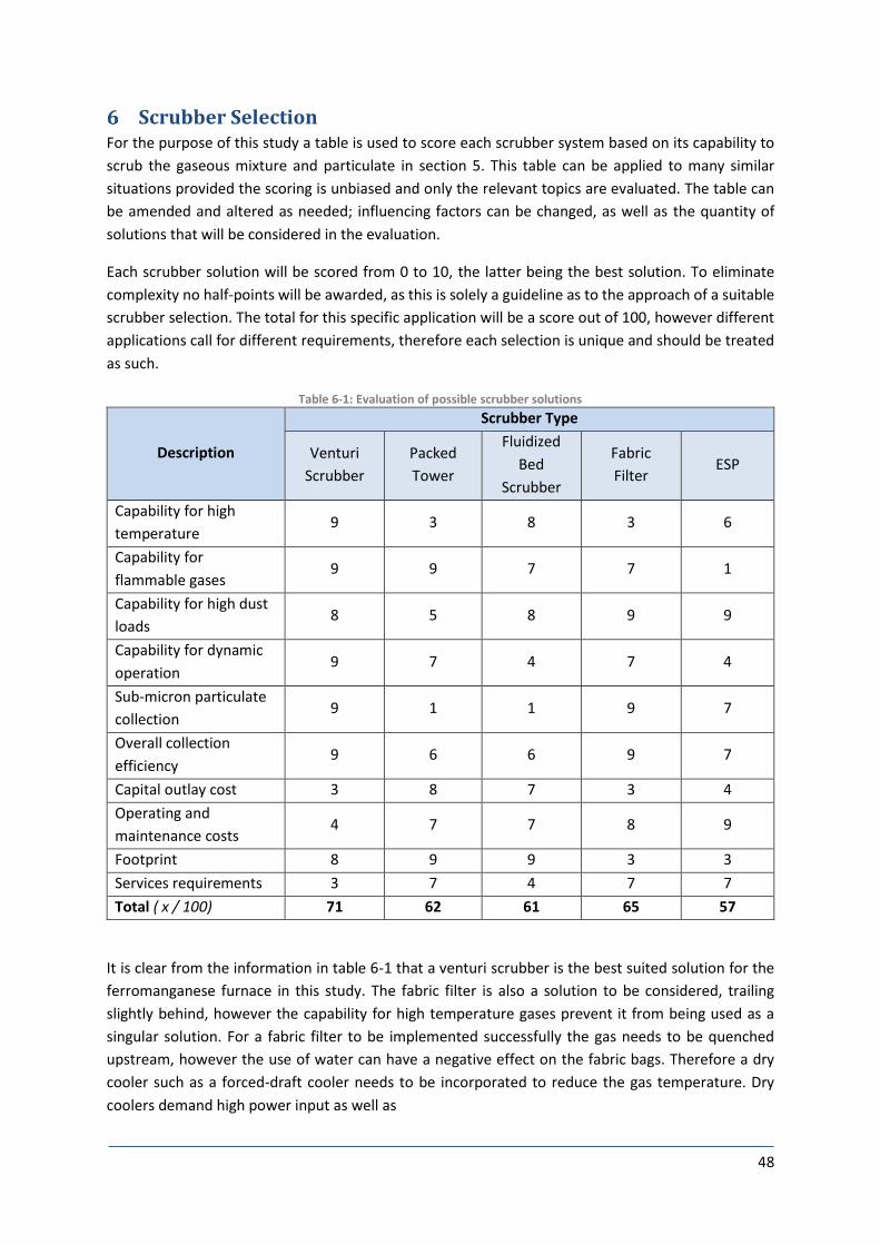
48
Scrubber Selection For the purpose of this study a table is used to score each scrubber system based on its capability to
scrub the gaseous mixture and particulate in section 5. This table can be applied to many similar
situations provided the scoring is unbiased and only the relevant topics are evaluated. The table can
be amended and altered as needed; influencing factors can be changed, as well as the quantity of
solutions that will be considered in the evaluation.
Each scrubber solution will be scored from 0 to 10, the latter being the best solution. To eliminate
complexity no half-points will be awarded, as this is solely a guideline as to the approach of a suitable
scrubber selection. The total for this specific application will be a score out of 100, however different
applications call for different requirements, therefore each selection is unique and should be treated
as such.
Table 6-1: Evaluation of possible scrubber solutions
Description
Scrubber Type
Venturi
Scrubber
Packed
Tower
Fluidized
Bed
Scrubber
Fabric
Filter ESP
Capability for high
temperature 9 3 8 3 6
Capability for
flammable gases 9 9 7 7 1
Capability for high dust
loads 8 5 8 9 9
Capability for dynamic
operation 9 7 4 7 4
Sub-micron particulate
collection 9 1 1 9 7
Overall collection
efficiency 9 6 6 9 7
Capital outlay cost 3 8 7 3 4
Operating and
maintenance costs 4 7 7 8 9
Footprint 8 9 9 3 3
Services requirements 3 7 4 7 7
Total ( x / 100) 71 62 61 65 57
It is clear from the information in table 6-1 that a venturi scrubber is the best suited solution for the
ferromanganese furnace in this study. The fabric filter is also a solution to be considered, trailing
slightly behind, however the capability for high temperature gases prevent it from being used as a
singular solution. For a fabric filter to be implemented successfully the gas needs to be quenched
upstream, however the use of water can have a negative effect on the fabric bags. Therefore a dry
cooler such as a forced-draft cooler needs to be incorporated to reduce the gas temperature. Dry
coolers demand high power input as well as

49
Fabric filters and ESPs require a large area for erection, as their collection efficiency is inversely
proportional to the velocity of the gas. To ensure that the gas moves as slowly as possible, the cross-
sectional area of the plant needs to be relatively large, increasing the overall footprint.
When considering a wet venturi scrubber it is important to understand the service requirements for
the cleaning of the gas. Process water is recycled in the scrubber plant, as it becomes contaminated
when exposed to the furnace off-gas. The outlet water from the scrubber plant is pumped to a settling
dam

50
Scrubber Design
7.1 Scrubber System A schematic diagram is always necessary when considering a system so that the properties of each
component can be designed accordingly. Once each component has been design the system needs to
be considered as a whole. Figure 7-1 indicates each component in the scrubber system and table 7-1
provides a brief description of each component with its corresponding number, each of which will be
discussed in detail in this section.
2
4
53
1
6
7
89
10
11
12
13
2021
14
17
16
19
18
23
15
24
Figure 7-1: Layout of scrubber system components Table 7-1: Scrubber components
Scrubber Components
1 Electric arc furnace 13 Main fan train
2 Emergency raw off-gas stack 14 Furnace pressure control damper
3 Emergency stack rotary water seal 15 Recirculation ducting
4 Raw gas flare 16 Distribution gas shut-off valve
5 Furnace over-pressure relief valve 17 Stack flow control damper
6 Raw off-gas transition duct 18 Clean gas stack
7 Primary venturi 19 Reflux water seal
8 Furnace water seal 20 Primary seal pot
9 High pressure venturi 21 Fan seal pot
10 Flooded elbow 22 Clean gas flare tip
11 Cyclonic separator 23 Emergency water tank
12 Differential pressure flow meter

51
7.2 Components in a Scrubber System
7.2.1 Electric Arc Furnace
At the start of the process, the electric arc furnace is the initial consideration when design the scrubber
plant. All the relevant information regarding the process that takes place within the furnace has been
discussed in Section 4.3.
There are, however, two addition aspects that need to be accounted for when considering the
ferromanganese smelting process, namely furnace over pressure and eruptions.
7.2.1.1 Furnace over pressure
This is a steady, but significant, positive increase of pressure within the furnace shell. It occurs as a
result of the ever changing dynamic reactions which take place during the smelting process. Figure 4-
5 clearly indicates the relationship between the CO yield and coke added. If a coagulation of coke was
to reduce a small quantity of manganese ore, it would result in an excess of CO gas.
Other mechanisms can also contribute to an excess of off-gas, especially when electrolysis of water
takes place, releasing large amounts of oxygen and hydrogen. The high internal furnace temperature
causes these gases to combust, also contributing to an increase in pressure. Water can exist from the
following sources:
Equipment in and around the furnace, such as
o Electrode cooling water leakages
o Overflow of the emergency stack rotary water seal
o Water cooled transition duct leakages
Inherent moisture in the reductant and ore
Moisture in the carbon paste used in the electrodes
7.2.1.2 Furnace Eruptions
Eruptions seldom occur, but are critical when designing safety features for the longevity of the plant.
During the smelting process, the less dense materials move upward in molten state. The lighter
materials are part of the slag, and are by-products of the process. The charged material in a
ferromanganese reduction process is at ambient temperature when the furnace is charged. There is a
significant temperature difference between the molten bed and the charged material, as indicated in
Figure 4-4, which can be as much as 1220°C.
The slag moves upward and further away from the electrode tip, which is the thermal source, and
starts to cool drastically. The slag then forms a crust between the hot molten bed and the cold charged
material due to the large temperature difference. The crust is capable of supporting a significant mass,
and therefore prevents the cold charge from moving downward; the void between the molten bed
and the crust increases. When the crust is no longer capable of supporting the mass, it collapses,
forcing the gas in the void upward with great force. The instantaneous pressure increase causes in a
large positive pressure underneath the furnace roof; the large area results in a massive upward force,
conforming to Pascal's law.
These eruptions are capable of displacing the furnace roof from its supports entirely, damaging nearby
equipment and putting a stop to production. Safety precautions need to be designed in the form of a

52
relief valve, which will be discussed in this section. The cost of repairs is enormous, exceeded only by
loss in production revenue.
7.2.2 Emergency Raw Off-Gas Stack
In the event of a system failure within the plant the emergency stack is used to relieve the furnace
from over pressurizing. The emergency stack is controlled by a rotary water sealing damper, which is
opened when triggered by an operator.
The scrubber system is designed for a specific operating condition of the furnace. When the furnace
operates outside of the range of the scrubber, other components such as the emergency stack are
enforced to ensure a safe operating environment. During the start-up and shut-down of the furnace,
a small quantity of gas is yielded which is less than the scrubber plant requires for stable operation.
During these low gas volume conditions, the emergency stack is opened and the scrubber plant is
sealed off to allow the furnace gas to be flared into the atmosphere. There are, however, strict
regulations regarding flaring to atmosphere, which include
Reason for flaring
Duration of flare
Furnace power input during flare
It is critical that these aspects are considered by the operating crew, as a furnace might be required
to flare to atmosphere at any given time; these procedures must be in place, and the requirements
must be adhered to.
7.2.3 Emergency Stack Rotary Water Seal
The rotary water seal is a high-temperature steel plate in the form of an arc which creates a seal in a
water bath to isolate the emergency stack. This water bath creates a perfect seal between the arc and
the duct inlet when closed. The head of water does not need to be significant, as the results from the
furnace pressure testing indicated a maximum pressure of 6.2mm.
To open the seal, the shaft needs to be turned 90 to break the seal and allow gas to pass through.
This arrangement allows for the plate to be retracted completely so that there are no obstructions in
the gas stream.
Another advantage of this seal arrangement is that the water can be continuously recycled, by adding
cold water at the bottom of the seal, and the hot water overflowing in a weir. The movement of water
induces cooling of the steel material, and also prevents settling of particulate in the bottom of the
water bath.
7.2.4 Raw Gas Flare
Legislation requires any flammable gas flared to atmosphere to be combusted. This is to ensure that
a cloud does not form above the plant, which could spontaneously combust. Also, CO can have adverse
health effects on people when inhaled, however this risk is eliminated when it is combusted, changing
it into CO2 gas. To combust this gas a high temperature flare igniter is used.
Figure 7-2 represents the components in a flare ignition system. When the gas enters the base
reduction in the flare diameter it is accelerated, increasing the exit velocity and thus forcing the base

53
of the flame farther from the tip. This ensures that the construction material remains relatively cool
and protection of the instrumentation. The tip is fitted with a serrated arrangement to induce a
pressure differential between the high velocity gas and the static, higher pressure air. The air is then
drawn towards the gas stream and mixes above the tip, allowing ignition to take place.
There are a set of igniters on either side of the flare, which each comprise of an LPG supply, high-
energy igniter and a thermocouple. The high-energy igniter is essentially a high voltage spark-plug,
which ignites the LPG projected through a nozzle. The igniter will continue sparking until the
thermocouple measures a significant temperature, confirming that combustion has started. The LPG
and power supply to the flare are then shut off, as it is a waste if they are used permanently.
The perforated cylinder around the flare is to eliminate the drag force of high speed winds. Typically
a flare can be as high as 60m in the air, which results in a massive moment on the supports at the base
support. The perforation induces a turbulent layer along the cylinder, reducing the pressure drop
across the cross-section area of the cylinder, thus reducing the applied force.
1
2
3
4
5
6
7
8
9
Components
1 – Thermocouple2 – LPG outlet3 – High energy igniter4 – Serrated tips5 – Perforated cylinder shell6 – Duct reducer7 – Duct8 – Terminal connector9 – Connection flange
Figure 7-2: Schematic of a flare tip ignition system
7.2.5 Furnace Over-Pressure Relief Valve
Over pressure, as discussed earlier, needs to be accounted for when designing safety features to
protect the plant. This component is designed specifically to relief the furnace from eruptions, which
demand a robust and fail-proof concept.
The relief valve is essentially a pressure vessel with an interior mushroom-shaped plate. The vessel is
filled with water and the plate forms a water seal. In the event of over pressure the water between
the mushroom and the inlet duct is displaced downwards, allowing gas to escape through to the

54
emergency stack. The pressure relief valve is always located next to the rotary water seal so that it
can be bypassed if necessary. A typical pressure relief valve design is indicated in Figure 7-3.
It is important to note that the hydraulic effect takes place in the water when displaced. The area
between the inlet duct and the mushroom must be significantly smaller than the area between the
mushroom and the vessel shell. This will ensure that relief pressure is not significantly increased when
the water is displaced. If the gas pressure in the duct is less than the water head in the relief valve,
nothing will be bypassed which can cause a rupture at a weak point in one of the other components.
Components
1 – Outlet duct2 – Relief valve shell3 – Mushroom seal4 – Water level5 – Weir6 – Inlet duct
H – Water headD – Outer diameterd – Inner diameter
H
d
D
1
2
3
4
6
5
Figure 7-3: Schematic of a furnace pressure relief bypass valve
7.2.6 Raw Off-Gas Transition Duct
The transition duct connects the furnace to the quench venturi, so as to transport the gas safely to the
scrubber plant. Due to high raw gas temperatures transitions duct needs to be design to withstand
both a high continuous operating temperature, as well as cater for possible eruptions and
temperature spikes. The ideal solution for this is a water cooled duct, which makes use of cooling
water within a jacket around the duct to continuously cool the duct temperature. A typical water
cooled duct is illustrated in Figure 7-4. The cold water inlet must always be lower than the outlet, so
that any steam that might have formed can escape. The water is generally under a high pressure, so
that the boiling point is increased.
There are, however, certain parameters that need to be monitored with this sort of equipment. The
shell temperature must never decrease below the dew point of the gas; this will prevent acidic build-
up on the duct wall, as well as induce scaling within the duct. It is critical to ensure that a proper mass

55
and energy balance is conducted when executing the design, as in equation 6-1 where ṁwater needs to
be solved.
�̇�𝑤𝑎𝑡𝑒𝑟𝐶𝑝𝑤𝑎𝑡𝑒𝑟(𝑇𝑖𝑛 − 𝑇𝑜𝑢𝑡) = �̇�𝑔𝑎𝑠𝐶𝑝𝑔𝑎𝑠(𝑇𝑖𝑛 − 𝑇𝑜𝑢𝑡) ( 7-1 )
Cold
Water
Inlet
Hot
Water
Outlet
Raw Gas
Flow
A A
Section A-A
1
2
Components
1 – Connecting flange2 – Water pipe shell
Figure 7-4: Schematic of a raw off-gas transition duct section
7.2.7 Primary Venturi
The first step in handling the gas stream in the scrubber plant is to cool it sufficiently to within
equipment capability. Hot gas is more expensive to handle, as it requires higher grade material, and
the volumetric flow rate of the gas is greater, demanding larger equipment.
The primary venturi, or quencher, makes use of liquid vapourisation to cool the gas stream. Additional
advantages include precipitation of gaseous volatiles and the eliminating a fraction of the particulate
matter. Generally, industrial evaporative cooler design is based on steam tables, however they are
rarely used for processes other that air (Spellman and Whiting, 2005). For this process, air is not
present in the gas stream, therefore the calculations need to be based on psychrometric principals.
Psychrometric charts are generated through experimentation by many different organisations,
however they are primarily researched for the HVAC industry, which is air based and below 50°C at
atmospheric pressure dependent on elevation. The CO rich gas stream in the ferromanganese
reduction process requires a specialised psychrometric chart, which in calculated in this section.

56
7.2.7.1 Psychrometrics
Pyschrometry is defined as the thermal and physical properties of gas-vapour mixtures (World
Meteorological Organisation, 2008). These properties are dependent on a range of factors, which
requires certain assumptions to be made before initiating the calculations.
The first step in determining the psychrometric properties of the gas, in to identify the liquid that will
be used to quench the stream. As discussed during the previous section, water will be used as the
scrubbing liquid, however other processes may require neutralisation of acidic or alkaline gas streams;
the applicable scrubbing liquid will then be evaluated in the same manner. Thereafter a Grosvenor
chart needs to be generated, which is a plot of temperature versus humidity ratio. The purpose of
calculating these values is to determine the mass of water that needs to be added to specific mass of
gas for the required cooling to take place.
Firstly, the Antoine equation, derived from the Clausius-Clapeyron equation, is used to determine the
vapour pressure of the liquid in equation 7-3 (Antoine, 1888). The Antoine coefficients A, B and C are
5.11564, 1687.537 and 230.17 respectively, and are empirical values. The vapour pressure is measure
in mmHg.
log10(𝑃𝑣𝑎𝑝) = 𝐴 −𝐵
(𝑇 + 𝐶 − 273.15)
( 7-3 )
Rearranging this equation returns the temperature for a known vapour pressure.
𝑇 =𝐵
𝐴 − log10 (𝑃𝑣𝑎𝑝)− 𝐶 + 273.15
( 7-4 )
The total pressure is described in equation 7-5.
𝑃𝑡𝑜𝑡 = 𝑃𝑎𝑡𝑚 + 𝑃𝑔𝑎𝑠 ( 7-5 )
Additional equations need to be solved to determine a basis for the cooling relationship. The partial
vapour pressure needs to be determined, as indicated in equation 7-6. The molecular mass of the gas
used in the equation is the average sampled in the previous section.
𝑃𝑣𝑎𝑝𝑝𝑎𝑟= 𝑃𝑡𝑜𝑡 (𝑚𝑙 ∙
𝑀𝑀𝑙
𝑀𝑀𝑔 + 𝑀𝑀𝑙) (
1
𝑔 ∙ 𝑆𝐺𝐻𝐺)
( 7-6 )
Equation 7-5 is then substituted into equation 7-6 to determine the temperature for a specific
humidity ratio.

57
𝑇 =
𝐵
𝐴 − log10 [𝑃𝑡𝑜𝑡 (𝑚𝑙 ∙𝑀𝑀𝑙
𝑀𝑀𝑔+𝑀𝑀𝑙) (
1
𝑔∙𝑆𝐺𝐻𝐺)]
− 𝐶 ( 7-7 )
To generate an accurate plot, the relative humidity (RH) should be calculated for a range of input
values. RH can be defined as the ratio of partial vapour pressure to equilibrium vapour pressure (Perry,
1998), indicated in equation 7-8.
∅ =𝑒𝑙
𝑒𝑙∗ × 100% ( 7-8 )
The humidity ratio is defined in equation 7-9.
𝑊 =𝑚𝑙
𝑚𝑔 ( 7-9 )
The relevant data to be calculated for the Grosvenor plot is indicated in table 7-2. The temperature
and humidity ratio are not single values. Temperature is a function of humidity ratio for a specified
RH.
Table 7-2: Temperature and humidity ratio to be calculated
Relative Humidity Temperature Humidity Ratio
100 % * (to be calculated) *
80.0 % * *
60.0 % * *
40.0 % * *
20.0 % * *
10.0 % * *
5.00 % * *
2.50 % * *
1.00 % * *
0.10 % * *
Example calculation:
Assumptions: ml = 0.1 kg; RH = 100%
𝑃𝑡𝑜𝑡 = 𝑃𝑎𝑡𝑚 + 𝑃𝑔𝑎𝑠
𝑃𝑡𝑜𝑡 = 84.5 + 0.01 = 84.51 kPa
𝑇 =
𝐵
𝐴 − log10 [𝑃𝑡𝑜𝑡 (𝑚𝑙 ∙𝑀𝑀𝑙
𝑀𝑀𝑔+𝑀𝑀𝑙) (
1
𝑔∙𝑆𝐺𝐻𝐺)]
− 𝐶
𝑇 =
1687.537
5.11564 − log10 [84.51 (0.1 ∙18.02
27.46+18.02) (
1
9.81∙13.59)]
− 230.17 = 21.11 °C

58
Once the series of values is determined for each RH value, the data can be plotted, with humidity ratio
on the y-axis and temperature on the x-axis. RH of 100% is the equivalent of the liquid's dew point and
is the maximum vapour capacity of a specific volume of gas; additional vapour will condense and form
precipitation. The RH values plotted are indicated in Figure 7-4.
Figure 7-5: Grosvenor plot for the required relative humidity values of water
7.2.7.2 Adiabatic Saturation
An adiabatic process can be defined as a process that takes place without the transfer of external heat
or matter (Caratheodory, 1909). Adiabatic saturation can therefore be described as the saturation that
takes place in a process without external heat transfer. The process occurring in this instance is the
exchange of energy between the hot gas and the water which is vapourized. When matter undergoes
a phase transition, latent heat is absorbed by the matter or the system (Pierre, 1998). An empirical
formula was derived through experiments by Rogers and Yau (1989) to determine the latent heat of
water as a function of temperature, indicated in equation (6-10), where temperature is T and the
formula is accurate for a water temperature range of -20C to 40C, in kJ/kg.
𝐿𝑤𝑎𝑡𝑒𝑟(𝑇) = 2500.8 − 2.36𝑇 + 0.0016𝑇2 − 0.00006𝑇3 ( 7-10 )
The water used in the scrubber plant is supplied by a settling dam, which is subject to atmospheric
temperature change. Water temperatures may vary significantly due to seasonal change, however an
average of 22.5C was measured and will be used for the calculations in this study.
To determine the amount of energy transferred between the water and the gas during vapourization,
an energy balance needs to be equated. Equation 7-11 indicates the enthalpy for the gas for a specific
heat capacity in kJ/kg.
ℎ𝑔𝑎𝑠 = 𝐶𝑃∆𝑇 ( 7-11 )

59
Substituting these two equations and rearranging the variables, equation 7-12 can be declared and
returns a result in kJ.
ℎ𝑔𝑎𝑠,𝑓 = 𝑚𝑔𝑎𝑠 ∙ ℎ𝑔𝑎𝑠,𝑖 − 𝑚𝑤𝑎𝑡𝑒𝑟 ∙ 𝐿𝑤𝑎𝑡𝑒𝑟 ( 7-12 )
Substituting equation 7-12 with equation 7-11 allows the temperature difference that occurred to be
determined.
∆𝑇𝑔𝑎𝑠 =𝑚𝑤𝑎𝑡𝑒𝑟 ∙ 𝐿𝑤𝑎𝑡𝑒𝑟
𝑚𝑔𝑎𝑠 ∙ 𝐶𝑃,𝑔𝑎𝑠 + 𝑚𝑤𝑎𝑡𝑒𝑟 ∙ 𝐶𝑃,𝑤𝑎𝑡𝑒𝑟
( 7-13 )
Once the temperature difference has been determined for a specific mass of water mwater it can be
subtracted from the initial gas temperature. This returns the final temperature for a finite value of
water, however the accuracy of the solution increases as mwater approaches zero. Equation 7-13 also
needs to be expanded as all the variables are dependent on the temperature of the thermodynamic
system at any given instance. Equation 7-14 returns the specific heat capacity of gas and liquid as a
function of temperature, where variables a0 through a4 are empirical values determined by Poling et
al (2001) and are indicated in table 7-3.
𝐶𝑃
0
𝑅= 𝑎0 + 𝑎1𝑇 + 𝑎2𝑇2 + 𝑎3𝑇3 + 𝑎4𝑇4 ( 7-14 )
Table 7-3: Specific heat coefficients and capacities at STP (adapted from Poling et al., 2001)
Specific Heat Capacities
Description a0 a1
[x10-3]
a2
[x10-5]
a3
[x10-8]
a4
[x10-11]
CP/R @ 298.15 K
[kJ/kg-K]
Carbon Monoxide 3.912 -3.913 1.182 -1.302 0.515 29.14
Carbon Dioxide 3.259 1.356 1.502 -2.374 1.056 37.13
Hydrogen 2.883 3.681 -0.772 0.692 -0.213 28.84
Oxygen 3.630 -1.794 0.658 -0.601 0.179 29.38
Nitrogen 3.539 -0.261 0.007 0.157 -0.099 29.12
Methane 4.568 -8.975 3.631 -3.407 1.091 35.69
Water 4.395 -4.186 1.405 -1.564 0.632 75.29
The specific heat capacity of an object is the ratio between the heat added and the resultant
temperature (Halliday et al., 2013). Water has three main different heat capacity values, dependent
on its phase, indicated in Figure 7-6.

60
Figure 7-6: Enthalpy of water at different phases
There are, however, limitations to equation 7-14, as the heat capacity of water changes below its
boiling point. Also, complete water vaporization does not occur below boiling point, as is it undergoes
a gas-vapour mixture, i.e. the quality predicts how much gas is capable of vapourizing the water.
Therefore, the more saturated the gas becomes below boiling point, the more difficult it is for
vapourization to occur.
The limitations of the water can be defined in equations 7-15 and 7-16.
For Tgas >99.98 𝐶𝑃 = (1
𝑀𝑀) (𝑎0 + 𝑎1𝑇 + 𝑎2𝑇2 + 𝑎3𝑇3 + 𝑎4𝑇4) ( 7-15 )
For Tgas ≤99.98 𝐶𝑃 = (1
�̅�) (𝑎0 + 𝑎1𝑇 + 𝑎2𝑇2 + 𝑎3𝑇3 + 𝑎4𝑇4) ( 7-16 )
Example calculation:
Assumptions: mg = 1 kg; ml = 0.0005 kg; Tg,i = 250C; Tw = 22.5C, Wi = 0
𝐿𝑤𝑎𝑡𝑒𝑟(𝑇) = 2500.8 − 2.36𝑇 + 0.0016𝑇2 − 0.00006𝑇3
𝐿𝑤𝑎𝑡𝑒𝑟(𝑇) = 2500.8 − 2.36(22.5) + 0.0016(22.5)2 − 0.00006(22.5)3 = 2447.8 kJ/kg
𝐶𝑃,𝑔𝑎𝑠 = 𝑣𝐶𝑂 ∙ 𝐶𝑃,𝐶𝑂 + 𝑣𝐶𝑂2
∙ 𝐶𝑃,𝐶𝑂2+ 𝑣𝐻2
∙ 𝐶𝑃,𝐻2+ 𝑣𝑂2
∙ 𝐶𝑃,𝑂2+ 𝑣𝑁2
∙ 𝐶𝑃,𝑁2+ 𝑣𝐶𝐻4
∙ 𝐶𝑃,𝐶𝐻4 = 2.31 kJ/kg-K
𝐶𝑃,𝑤𝑎𝑡𝑒𝑟 = (
1
�̅�) (𝑎0 + 𝑎1𝑇 + 𝑎2𝑇2 + 𝑎3𝑇3 + 𝑎4𝑇4) = 1.86 kJ/kg-K
𝑇𝑓,𝑔𝑎𝑠 = 𝑇𝑖,𝑔𝑎𝑠 −
𝑚𝑤𝑎𝑡𝑒𝑟 ∙ 𝐿𝑤𝑎𝑡𝑒𝑟
𝐶𝑃,𝑔𝑎𝑠
𝑇𝑔𝑎𝑠 = 250 −
(0.0005 × 2447.8)
2.31 = 249.47 C

61
The assumptions in the calculation are that the gas is dry, i.e. there is no CP value for inherent water
in the gas. Therefore the latent water energy is only divided by the heat capacity of the gas, however
this changes when gas in vapourized, as the water mass within the gas increases as the gas cools,
altering the resultant heat capacity.
These equation need to be applied to the gas stream for each finitely small addition of water. The
resultant equation is thus the initial temperature less the sum of all the temperature differences,
which must be solved numerically, where Xl is the water quality in a gas-vapour mixture and only
applies when T < Tboiling.
𝑇𝑠𝑎𝑡 = 𝑇 − ∑𝛿 ∙ 𝐿𝑤𝑎𝑡𝑒𝑟
𝑚𝑔𝑎𝑠 ∙ 𝐶𝑃(𝑖−1),𝑔𝑎𝑠 + 𝑚𝑤𝑎𝑡𝑒𝑟 ∙ 𝐶𝑃(𝑖−1),𝑤𝑎𝑡𝑒𝑟(
1
1 − 𝑋𝑙)
𝑇𝑠𝑎𝑡=𝑅𝐻100
𝑖=1
( 7-17 )
Adiabatic saturation lines can be plotted over the Grosvenor plot in Figure 7-4 at different initial
temperatures. For the purpose of this study, 200C, 800C and 1 100C were used to plot three
adiabatic saturation lines for, indicated in Figure 7-7. The change in the vapourization efficiency of
water is clearly visible below the boiling temperature.
Figure 7-7: Grosvenor plot including adiabatic saturation lines
7.2.7.3 Applied Adiabatic Saturation
For the design of the scrubber in this study, the average gas temperature in the furnace will be used
as an operating condition, and both the minimum and maximum temperatures will be evaluated to
determine whether the psychrometric method is capable of quenching the gas.
When substituting the range of gas temperatures in table 5-2 into equation 7-17, a saturated gas
temperature for each initial gas temperature in returned in table 7-4. These values will then be
compared with the final experimentation to determine the accuracy of the design.

62
Table 7-4: Initial gas temperature vs. saturated gas temperature
Gas Temperatures
Description
Initial
Temperature
[C]
Saturated
Temperature
[C]
Liquid
Added
[kg/kg]
Average 310.50 41.38 0.26
Maximum 497.90 49.61 0.40
Minimum 244.00 37.34 0.21
7.2.7.4 Component Design
The primary venturi is a component that must be designed to withstand both high temperatures, and
a large volumetric gas flow rate. The actual flow rate of the gas increases with temperature (Clapeyron,
1834), thus the volumetric flow rates of the gas before and after the primary venturi need to be
calculated for sizing of the inlet and outlet. If the gas velocity is too low, particulate will drop out of
the gas stream in the connecting ducting, causing build-up and unnecessary maintenance demands. If
the gas velocity is too high, the dynamic pressure in the system increases significantly, demanding
higher power input and increasing the operating costs. Figure 7-8 indicates a typical layout for a
primary venturi.
Components
1 – Flange2 – Tangential water inlet3 – Differential pressure meter4 – Reduction5 – Venturi blade shaft6 – Venturi housing7 – Blade open position8 – Blade operating position9 – Expansion
A – Throat areaƟ – Inlet angle
1
2
3
4
6
7
8
9
5
A
Ɵ
Figure 7-8: Schematic of the primary venturi
To determine the gas volume before and after the primary venturi, the gas density needs to be
calculated and then the ideal gas law needs to be applied, indicated in equation 1-1. To determine the
gas density, equation 7-18 is applied.

63
𝜌 =𝑃 𝑀𝑀𝑔
𝑅 𝑇 ( 7-18 )
Table 7-5: Ratio between the inlet and outlet gas volumetric flow rate
Gas Flow Rate
Description Volume Flow
[Nm3/s]
T=310.50C T=35.78C
Density
[kg/m3]
Flow
[Am3/s]
Density
[kg/m3]
Flow
[Am3/s]
Carbon Monoxide 61.24 % 2.690 0.5978 5.749 1.129 3.043
Carbon Dioxide 12.74 % 0.559 0.9392 1.196 1.774 0.633
Hydrogen 9.77 % 0.429 0.0430 0.917 0.081 0.485
Oxygen 1.10 % 0.043 0.6829 0.103 1.290 0.054
Nitrogen 14.4 % 0.632 0.5979 1.352 1.129 0.715
Methane 0.71 % 0.003 0.3424 0.066 0.646 0.035
Total 100 % 4.392 9.384 4.967
From table 7-5 the ratio between the gas inlet and outlet volumetric flow rate can be defined as Qi :
Qo, which can be applied to the inlet and outlet area to maintain a constant velocity before and after
the primary venturi.
Once the flow rate through the primary venturi has been determined, a calculation needs to be done
to ensure that the injected liquid is sufficiently vapourized to ensure efficient quenching. Boll et al.
(1974) derived an equation for droplet size as a function of relative gas velocity, indicated in equation
7-19.
𝑑𝑙𝑖𝑞 =
4.22𝑒−2 + 5.77𝑒−3 (1000𝑄𝑙
𝑄𝑔)
1.922
𝑣𝑟𝑡ℎ1.602 ( 7-19 )
This is a complex calculation as the velocity in in the primary venturi throat is unknown, therefore it
needs to be solved iteratively with an additional set of equations. To determine the required
equations, the thermodynamic properties of liquid needs to be evaluated and then applied to the
vapourization process. The liquid droplets are subject to a convective heat transfer in the primary
venturi, and therefore equation 7-20 can be utilized, where dliq is the droplet diameter.
𝑞 = 𝐴𝑙𝑖𝑞 ∙ 𝑘 ∙ 𝑑𝑙𝑖𝑞∆𝑇 ( 7-20 )
𝑘 =
1
2(𝑘𝑙𝑖𝑞 + 𝑘𝑔𝑎𝑠)
( 7-21 )
For this equation, we can assume that q is equal to the latent vapourization heat of water, kgas is the
sum of the weighted thermal conductivity coefficients for the gases present, and T is the

64
temperature difference calculated in table 7-4. Therefore the only variables required are the liquid
surface area and the droplet diameter. These are both a function of equation 7-19 as the liquid surface
area and the liquid volume are indicated in equations 7-21 and 7-22 respectively.
𝐴𝑠𝑝ℎ𝑒𝑟𝑒 = 𝜋𝑑2 ( 7-22 )
𝑉𝑠𝑝ℎ𝑒𝑟𝑒 =1
6𝜋𝑑2 ( 7-23 )
𝑁𝑑𝑟𝑜𝑝𝑙𝑒𝑡𝑠 =𝑄𝑙𝑖𝑞
𝑉𝑠𝑝ℎ𝑒𝑟𝑒
( 7-24 )
𝑄𝑙𝑖𝑞 = 𝑊 ∗ 𝑚𝑔𝑎𝑠̇ ( 7-25 )
The pressure drop across a venturi throat is a function of velocity and liquid-to-gas ratio, which is
indicated in equation 7-26 (adapted from Hesketh, 1986).
∆𝑃 = (𝑣𝑡ℎ
2 𝜌𝑔
1.879) 𝐴𝑡ℎ
0.133 [0.56 +16.6𝑄𝑙
𝑄𝑔+ 40.7 (
𝑄𝑙
𝑄𝑔)
2
] ( 7-26 )
The volume of liquid added to the gas in table 7-4 can be divided by the volume of the droplet in
equation 7-22. This will result in the total number of droplets in the gas stream, assuming they are all
of equal diameter. Subsequently equation 7-25 can be used to determine total pressure drop across
the primary venturi throat. By substituting each of these equations into an iterative calculation, the
results returned are indicated in table 7-6.
Table 7-6: Results returned to determine the throat velocity
Variable Result Unit
k 0.12773 W/m-K
q 2 447.80 W
T 274.70 C
A liq 1 400.00 m2
N droplets 3.884 x10¹⁰ -
A sphere 3.605 x10⁻⁸ m2
V sphere 6.43 x10⁻¹³ m3
v th 66.50 m/s
dl 5.106 x10⁻⁵ m
P 2 248.00 Pa
A throat 0.4377 m2
As discussed earlier, the collection efficiency in a venturi scrubber is dictated by the pressure drop
across the throat. The primary venturi is designed to quench the hot gas stream, however there is a

65
secondary benefit of this equipment. The pressure drop generated for the atomization of the liquid
also contributes towards the collection of particles.
7.2.8 Furnace Water Seal
In the event of an emergency, the first priority is to isolate the furnace from the extraction of the
primary off-gas scrubber. Due to the high temperature of the off-gas and the safety hazards paired
with the escape of carbon monoxide, it is difficult to isolate the furnace with a mechanical shut-off
valve or spade. During the movement of a mechanical valve gas can easily escape to atmosphere, or
air can be drawn into the gas stream resulting in an explosion.
To account for furnace isolation during certain events a mechanism needs to be implemented that can
withstand the immense heat, as well as positively seal the interconnecting duct without the risk of gas
escape or ingress. An apt solution is a barometric water seal, which incorporates water within a vessel
to obtain a pressure head, as well as maintain a cool surface on the mechanical equipment in the
presence of hot gas. A typical arrangement for a water seal is indicated in Figure 7-9.
Components
1 – Primary venturi2 – Cold gas outlet3 – Water seal4 – Vessel shell5 – Impingement plate6 – Water outlet
H – Water sealing height
1
2
3
4
6
5
H
Figure 7-9: Schematic of a furnace water seal
The water seal makes use of a simple sealing mechanism, in which the head of water creates a positive
seal greater than the furnace can supply, or that which the scrubber can extract. The equation for this
sealing pressure is indicated in equation 7-27, where H is in metres.
𝑃 = 𝜌𝑤𝑎𝑡𝑒𝑟 𝑔 𝐻 ( 7-27 )
The operation of the water seal is simple and near impossible to fail. A spring-loaded isolation valve is
located bellow the water outlet at the bottom of the water seal. The valve is fail-closed, meaning that

66
it will use the force of the spring to close if the compressed air or electrical supply were to fail. In
addition to the water supply from the primary venturi, a second water supply continuously feeds the
water seal at a high flow rate. Once the isolation valves has closed the water level within the vessel
will begin to rise until it overflows to the outlet. The difference in height between the bottom of the
seal and the outlet duct dictates the sealing pressure capability of the water seal.
The water seal is a dual purpose component, as it serves a purpose for dust collection in addition to
the main isolation mechanism. Elimination mechanisms discussed in Section 2 are applied in this piece
of equipment, specifically targeting interception and diffusion. This can be described as the
phenomena that occurs when a particle has been attached to a liquid droplet, but requires a significant
impact to force the particle within the surface of the droplet. To cause this impact an impingement
plate is inserted bellow the water seal outlet, directly below the primary venturi.
The inner water seal is significantly narrower and has less sectional area than the outer vessel. This
allows the gas to move at a high speed when exiting the primary venturi, but decelerates when moving
upward toward the outlet. This upward velocity is based on the force of the moving gas on the droplet
as a function of aerodynamic diameter. This allows the droplets which contain particulate to drop out
of the gas stream before reaching the outlet. Particulate collection is not the primary goal when
designing the primary venturi and water seal, however their properties can be utilized to design more
compact and efficient systems.
7.2.9 High Pressure Venturi
By the time the gas reaches the high pressure venturi (HPV) it has been quenched and a large portion
of the particulate matter has been removed. It is clear, however, that a large portion of the PSD
indicated in Section 5 is smaller than 2 µm; these will not be remove efficiently by the primary venturi,
hence the implementation of a venturi with a greater pressure drop.
To determine exactly how much particulate needs to be removed, a calculation needs to be done to
determine the mass for each PSD range. The HPV is will be designed according to the particulate
elimination determined as a function of mass, as legislative rules dictate emission limits in mg/m3. The
results are indicated in table 7-7, and are calculated by multiplying the PSD ranges with the dust load
in the gas. This calculation is only conducted for the operating furnace power input of 42 MW.
Table 7-7: Weighted PSD at 42 MW furnace load
Particle Size Distribution
PSD Range Percentage Dust Load
[mg/Nm3]
Gas Yield
[Nm3/s]
Dust Yield
[mg/s]
Weighted
[mg/Nm3]
< 1 µm 2.60 % 37 775.13 4.393 4 314.59 982.15
1 µm – 2 µm 20.34 % 37 775.13 4.393 33 753.44 7 683.46
2 µm – 5 µm 45.51 % 37 775.13 4.393 75 522.09 17 191.46
5 µm – 10 µm 22.86 % 37 775.13 4.393 37 935.28 8 635.39
> 10 µm 8.68 % 37 775.13 4.393 14 404.16 3 278.88

67
0.01
0.05
0.10
0.20
0.50
1.00
2.00
5.00
10.00
20.00
30.00
40.00
50.00
60.00
70.00
80.00
90.00
95.00
98.00
99.00
99.95
99.98
99.90
99.99
0.1
0.2
0.3
0.4
0.5
0.6
0.7
0.8
0.9
1.0
2.0
3.0
4.0
5.0
6.0
7.0
8.0
9.0
10
0.01
0.05
0.10
0.20
0.50
1.00
2.00
5.00
10.00
20.00
30.00
40.00
50.00
60.00
70.00
80.00
90.00
95.00
98.00
99.00
99.95
99.98
99.90
99.99
Pe
rce
nta
ge
Lo
st
Pe
rce
nta
ge
Re
mo
ve
d
Aerodynamic Diameter
[μm]
Pre
ssur
e dr
op in
a re
ctan
gular v
entu
ri
[kPa]
1.70
2.50
3.70
5.00
6.20
8.70
12.4
Figure 7-10: Venturi collection efficiency as a function of particle diameter and pressure drop (adapted from Hesketh, 1986)
To design a scrubber plant accurately, the particle size distribution (PSD) needs to be determined. The
collection efficiency of a venturi is a function of the PSD, indicated in equation 7-28 and 7-29, where
dp2 is the particle diameter (Spellman and Whiting, 2005). It is clear from both the equations and Figure
7-10 that the venturi collection efficiency is proportional to the particle’s aerodynamic diameter.
𝜂 = 1 − 𝑒(−𝑘𝑅√𝜓) ( 7-28 )
𝜓 = 𝑑𝑎𝑒𝑟
2 𝜌𝑝 𝑉𝑡
9 𝜇𝑔 𝑑𝑙
( 7-29 )

68
7.2.9.1 Component Design
There are many aspects to consider when designing the high pressure venturi, all of which are critical
to ensure that the collection efficiency is sufficient for the required mass of particulate to be removed
from the gas stream. The HPV has a very similar arrangement to that of the primary venturi, however
it is significantly narrower to accelerate the gas to achieve the increase in gas velocity. A typical
arrangement of an HPV is indicated in Figure 7-11.
Components
1 – Flange2 – Tangential water inlet3 – Differential pressure meter4 – Reduction5 – Venturi blade shaft6 – Venturi housing7 – Blade open position8 – Blade operating position9 – Expansion
A – Throat areaƟ – Inlet angle
1
2
3
4
6
7
8
9
5
A
Ɵ
Figure 7-11: Schematic of a high pressure venturi
Legislation dictates that 100 µm/Nm3 is the maximum allowable emissions for an industrial
application. To determine a collection efficiency to achieve this, the allowable rate can be divided by
the total dust load, returning a value of 99.735%. This can rather be recalculated to eliminate a
required percentage of the submicron particles, assuming a collection efficiency of the larger particles
to be 100%. This returns a value of 89.81% for particles smaller than 1 µm. This is the efficiency that
will be designed for regarding the HPV.
When considering the collection efficiency of a wet venturi scrubber, the Johnstone equation can be
used, as indicated in equation 7-30, where K is a geometrical particle constant and ψ is the inertial
impaction parameter and is defined in equation 7-31. This equation substitutes the aerodynamic
diameter with the actual diameter by decreasing the inertial impaction parameter by a factor of two.
𝜂 = 1 − 𝑒(−𝐾(𝑄𝑙/𝑄𝑔)√𝜓) ( 7-30 )

69
𝜓 =𝐶 𝑑𝑝
2 𝜌𝑝 𝑣𝑡
18 𝜇𝑔 𝑑𝑙
( 7-31 )
To account for effects on small particles the Cunningham correction factor C is applied, which is a
derivation of Stokes’ law, and indicated in equation 7-32 (Cunningham, 1910).
𝐶 = 1 +𝑇(6.21 × 10⁻⁴)
𝑑𝑝
( 7-32 )
Equation 7-30 can be declared equal to 89.81% where dl = 1 µm; subsequently equation 7-31 can be
substituted to find the value for Vt, the throat velocity. These equations are to ne solver iteratively
with the properties for the particulate from Section 5. The inertial impaction parameter is a function
of particulate density, where the efficiency is proportional to the density, indicated in Figure 7-12
where the series is plotted using the aforementioned equations.
Figure 7-12: Collection efficiency of a wet venturi scrubber vs particulate density
To ensure that the scrubber is designed for the worst possible case, the particulate with the least
density will be used, i.e. carbon, which has a density of 1.9 g/cm3. If there is a smaller mass fraction of
carbon in the gas stream the collection efficiency will increase. This assumption is critical, as the dust
yield is not fixed and firm; fluctuations are prominent and need to be accounted for in the design to
ensure that legislative rules are adhered to.
According to Rudnick et al. (1986) the optimal liquid-to-gas ratio for particulate removal is 0.936 and
1.337 m3/1000. The L/G for study is chosen as 1.337, as it is the maximum value for optimal collection,
0.0000
0.1000
0.2000
0.3000
0.4000
0.5000
0.6000
0.7000
0.8000
0.9000
1.0000
0 2000 4000 6000 8000 10000
Co
llect
ion
Eff
icie
ncy
Density[kg/m³]
Collection Efficiency

70
however the liquid input is greater allowing a thicker film on the internal surfaces of the HPV. This
helps to decrease wear on the internal surfaces, prolonging the life of the scrubber.
The variable and equation discussed are applied to determine the design criteria for the HPV. As with
the primary venturi it is important to calculate the gas velocity required and subsequently the venturi
throat area. These two parameters are critical for a detail design of the component to be done. The
results returned from the calculations are indicated in table 7-8.
Table 7-8: Results returned to determine the throat velocity
Variable Result Unit
ɳ 0.8981 -
K 0.171 -
dp 1.0 x10⁻⁶ m
Tgas 308.2 K
C 1.191 -
QL/QG 1.337 -
ρgas 1.107 kg/m3
ρp 1900.00 kg/m3
µgas 1.802 x10⁻⁵ Pa.s
v th 181.7 m/s
dl 1.271 x10⁻⁵ m
p 18 270.00 Pa
A throat 0.0273 m2
To ensure that the resulting values are suitable for the scrubber, each PSD range needs to be evaluated
with the calculated velocity. The collection efficiency for each PSD range is indicated in table 7-9,
where vth is equal to 181.7 m/s. The primary venturi also contributes towards the total collection
efficiency, and needs to be incorporated in the calculations.
Table 7-9: Collection efficiency for each PSD range
Collection Efficiency
PSD Range
Collection
Efficiency
Weighted
[mg/Nm3]
Residual
[mg/Nm3]
Primary Venturi
< 1 µm 52.49 % 982.15 466.61
1 µm – 2 µm 74.88 % 7 683.46 1 930.08
2 µm – 5 µm 92.94 % 17 191.46 1213.71
5 µm – 10 µm 99.84 % 8 635.39 13.81
> 10 µm 100.0 % 3 278.88 0.00
Total 3 624.21
High Pressure
Venturi
< 1 µm 89.98 % 466.61 47.45
1 µm – 2 µm 96.44 % 1 930.08 24.12
2 µm – 5 µm 100.0 % 1213.71 0.00
5 µm – 10 µm 100.0 % 13.81 0.00
> 10 µm 100.0 % 0.00 0.00
Grand Total 71.57

71
The resultant emission is allowable for the scrubber plant, as it falls within the average emission rate.
The results in table 7-9 are still conservative, as the density used was that of carbon, meaning that the
collection efficiency will most definitely be higher in practicality. It is impossible to calculate exactly
what the throat velocity needs to be, as the particulate composition per unit of gas fluctuates.
7.2.9.2 Venturi Control
During start-up of the scrubber only a small quantity of gas passes through the system. The venturi
therefore needs to be dynamic to change the resistance of the system to prevent a system stall. An
actuator is attached to the shaft of the venturi blade, which keeps it in a fully open position until the
scrubber has reached an equilibrium and then proceeds to close to its operating position.
To determine an actuator size and a shaft diameter, a simple calculation can be done to determine
the force on the blade and subsequently the moment require to operate it. Equation 7-33 indicates
the equation used to determine these forces.
𝑀 = (1
2𝜌𝑐𝑣𝑔
2) (𝐴𝑏𝑙𝑏
𝑐𝑜𝑠𝜃
2) ( 7-33 )
7.2.10 Flooded Elbow
As discussed in the furnace water seal design, impingement is critical when a particle attaches to a
liquid droplet as a result of interception or diffusion. Impingement plates often wear quickly due to
the abrasive nature of the particulate, however there are solutions to impinge without the risk of
wear. A flooded elbow is implemented, which is essentially a duct elbow with a water bed.
When the gas is accelerated downward in the high pressure venturi, the droplets have more inertia
than the gas, making it harder to change direction with the gas stream. These droplets continue with
a downward trajectory, and collides with the water’s surface. This impact allows the particle to move
into the liquid droplet before it exits the elbow. Figure 7-13 indicates a typical arrangement of a
flooded elbow.

72
Components
1 – High pressure venturi2 – Cold gas outlet3 – Water seal4 – Vessel shell5 – Impingement plate6 – Water outlet
1
2
3
6
5
4
Figure 7-13: Schematic of a flooded elbow
Problems can be experienced with flooded elbows if they are not designed correctly. If the water bed
is too deep, the gas forces the liquid outward toward the side walls, resulting in a large meniscus
shaped water surface. The water will deform to suit the flow pattern of the gas, eliminating a proper
impingement surface. To account for this, steel protrusions can be inserted in the water bed,
preventing the outward movement of water. This increases the impaction efficiency while still
maintaining a water film on the steel surface to prevent wear.
The difference between a water bed with and without steel protrusion is indicated in Figure 7-14.
Water is constantly pumped into the flooded elbow to prevent settlement between the steelwork as
well as maintaining a filled water level.

73
Wet elbow with impingement plates Wet elbow without impingement plates
Figure 7-14: Comparison of a flooded elbow with and without impingement plates

74
7.2.11 Cyclonic Separator
Once the particulate has been forced into the liquid droplet, the majority of the droplets will still be
in the gas stream, which need to be separated from the gas stream. A cyclonic separator is used in
these scrubbers to eliminate the droplets by applying the law of centrifugal force. Figure 7-15 indicates
a typical layout for a cyclonic separator.
Components
1 – Separator2 – Conical diffuser3 – Separator shell4 – Gas inlet5 – Water outlet6 – Cyclonic air flow pattern
H – Cyclone heightD – Cyclone diameterS – Outlet heightDe – Outlet diameter
1
2
3
5
4
6
H
D
S
De
Figure 7-15: Schematic of a cyclonic separator
Designing the cyclonic separator requires a separation efficiency to be calculated. To initiate these
design calculations, the number of revolutions in the separator needs to be determined, as indicated
in equation 7-34.
𝑁 =1
𝐻𝑖(𝐻 +
𝑆
2)
( 7-34 )
For the droplets to be collected, they must strike the outer shell of the separator while the gas moves
across it within a certain amount of time. This time duration can be described as the gas residence
time, and is defined in equation 7-35.
∆𝑡 =𝜋 𝐷 𝑁
𝑣𝑔
( 7-35 )

75
When the droplet enters the separator it is rapidly accelerated until it reaches its terminal velocity in
a radial direction. The terminal velocity required to remove the droplet within a given time a certain
distance r away from the shell. This is defined in equation 7-36.
𝑣𝑡 =𝑟
∆𝑡
( 7-36 )
The droplet drift velocity then needs to be determined as a function of droplet size.
𝑣𝑡 =(𝜌𝑙 − 𝜌𝑔)𝑑𝑙
2𝑣𝑔2
9 𝜇 𝐷 ( 7-37 )
Substituting equation 7-35 into 7-36 eliminates t, and allows the equation to be rearranged to
determine the droplet diameter dl, indicated in equation 7-38.
𝑑𝑙 = [9 𝜇 𝑟
𝜋 𝑁 𝑣𝑔(𝜌𝑙 − 𝜌𝑔)]
1
2
( 7-38 )
Equation 7-38 indicates the smallest droplet size in a cyclonic separator that will be collected with
100% efficiency. Lapple (1951) derived an equation for the collection of 50% of the droplets described
in equation 7-38, and is expressed in equation 7-39, where dlc is the “cut diameter of 50%.
𝑑𝑙𝑐 = [9 𝜇 𝑟
2𝜋 𝑁 𝑣𝑔(𝜌𝑙 − 𝜌𝑔)]
1
2
( 7-39 )
The collection efficiency is expressed in equation 7-40 for the droplet size.
𝜂 =1
1 + (𝑑𝑙𝑐
𝑑𝑙)
2 ( 7-40 )
When considering the cyclonic separator as a component in the scrubber system, the pressure loss
needs to be calculated to determine a pressure balance across the system. The pressure drop is
expressed in equation 7-41, and was developed by Shepherd and Lapple (1939), where H is based
on the cyclone dimension ratios and was developed by Dirgo (1988) and Ramachandran et al. (1991)
and is expressed in equation 7-42, where a and b are the inlet dimensions.
Δ𝑝𝑐 = ∆𝐻 (𝜌𝑔
𝑣𝑖2
2)
( 7-41 )

76
A range of standard designs was developed to initiate a cyclone design by assuming geometrical ratios,
which are indicated in table 7-10.
Table 7-10: Standard dimension ratios for cyclone design (Liu, 1997)
Duty Derived D a/D b/D De/D S/D h/D H/D B/D ΔH
High Efficiency Stairmand 1 0.50 0.20 0.50 0.50 1.5 4.0 0.375 5.4
High Efficiency Swift 1 0.44 0.21 0.40 0.50 1.4 3.9 0.40 9.2
General Purpose Lapple 1 0.50 0.25 0.50 0.63 2.0 4.0 0.25 8.0
General Purpose Swift 1 0.50 0.25 0.50 0.60 1.75 3.75 0.40 7.6
Consensus Stern et al. 1 0.45 0.20 0.50 0.63 0.75 2.0 - -
High Volume Stairmand 1 0.75 0.38 0.75 0.88 1.5 4.0 0.38 7.2
High Volume Swift 1 0.80 0.35 0.75 0.85 1.7 3.7 0.40 7.0
∆𝐻 = 20 (𝑎𝑏
𝐷𝑒2) [
(𝑆
𝐷)
(𝐻
𝐷) (
ℎ
𝐷) (
𝐵
𝐷)
] ( 7-42 )
A high efficiency and high volume cyclone was derived by Stairmand (1951) and Swift (1969). A general
purpose cyclone was derived by Lapple (1951) and Swift (1969), and a consensus was derived by Stern
et al. (1956).
Due to the liquid droplet size generated in the high pressure venturi a high efficiency cyclone will be
used. The Stairmand derivation is selected, as the H value is less than that of Swift, which reduces
the pressure drop across the cyclone, subsequently reducing the power consumption required to
displace the gas. The sacrifice in efficiency is negligible compared to the power that is saved.
By substituting the ratios derived by Stairmand into equation 7-42 and solving the previous cyclone
equations iterative, the results returned are indicated in table 7-11.
Table 7-11: Results to determine the pressure drop across the cyclone
Variable Result Unit
dL 1.271 x10⁻⁵ m
H 4.63 -
N 12 -
t 476 s
vg 14.89 m/s
vt 2.101 x10⁻⁵ m/s
ρgas 1.107 kg/m3
ρliq 1900.00 kg/m3
µgas 1.802 x10⁻⁵ Pa.s
pc 568 Pa
ɳ 66.7 %

77
The pressure drop pc will be used in the power requirement calculation is section 7.2.13. The
elimination efficiency ɳ of the cyclone is a low value only in the event that droplets do not attached
to each other before reaching the cyclone. The flooded elbow induces droplet merging, which
increases the cyclone efficiency. The value in table 7-11 is the worst case efficiency, and therefore the
assumption can be made that ɳ > 66.7%.
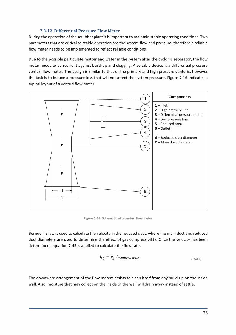
78
7.2.12 Differential Pressure Flow Meter
During the operation of the scrubber plant it is important to maintain stable operating conditions. Two
parameters that are critical to stable operation are the system flow and pressure, therefore a reliable
flow meter needs to be implemented to reflect reliable conditions.
Due to the possible particulate matter and water in the system after the cyclonic separator, the flow
meter needs to be resilient against build-up and clogging. A suitable device is a differential pressure
venturi flow meter. The design is similar to that of the primary and high pressure venturis, however
the task is to induce a pressure loss that will not affect the system pressure. Figure 7-16 indicates a
typical layout of a venturi flow meter.
Components
1 – Inlet2 – High pressure line3 – Differential pressure meter4 – Low pressure line5 – Reduced area6 – Outlet
D – Reduced duct diameterD – Main duct diameter
1
2
3
4
6
5
d
D
d
Figure 7-16: Schematic of a venturi flow meter
Bernoulli’s law is used to calculate the velocity in the reduced duct, where the main duct and reduced
duct diameters are used to determine the effect of gas compressibility. Once the velocity has been
determined, equation 7-43 is applied to calculate the flow rate.
𝑄𝑔 = 𝑣𝑔 𝐴𝑟𝑒𝑑𝑢𝑐𝑒𝑑 𝑑𝑢𝑐𝑡 ( 7-43 )
The downward arrangement of the flow meters assists to clean itself from any build-up on the inside
wall. Also, moisture that may collect on the inside of the wall will drain away instead of settle.

79
7.2.13 Main Fan Train
The fans can be described as the “heart” of the scrubber plant, as they allow the movement of gas to
take place. Fan operation in the plant is critical, as production of the furnace cannot commence at full
load if the scrubber plant is offline. Two fain trains are typically installed in parallel with change-over
valves, of which one train is for stand-by. This also assists with maintenance and servicing of the fans
or during repairs.
Fan selection is a simple process, which is governed by the gas power required to operate. This is
defined in equation 7-44, where psys is the total pressure across the scrubber system and Qc is a
contingency for stability.
𝑃𝑔 = (𝑄𝑔 + 𝑄𝑐)𝑝𝑠𝑦𝑠 ( 7-44 )
Due to the fluctuations in furnace pressure a gas flow rate contingency is incorporated into the gas
power requirement. This allows the fans a larger range of control, as the gas can be recirculated if the
furnace yields less gas, or extract more gas if the yield is greater.
The electrical power demand of the process is the incorporated efficiency of the fan and the electrical
motor into equation 7-42, and is expressed in equation 7-45.
𝑃𝑔 =(𝑄𝑔 + 𝑄𝑐)𝑝𝑠𝑦𝑠
𝜂𝑓𝑎𝑛𝜂𝑚𝑜𝑡𝑜𝑟
( 7-45 )
The total system pressure needs to be determined to evaluate the fan selection. Each component’s
pressure loss is indicated in table 7-12.
Table 7-12: Pressure losses of each system component
Component Pressure Loss
[Pa]
Flow Rate
[Am3/s]
Gas Power
[kW]
Primary venturi 2 448.00 4.965 12.15
Furnace water seal 258.00 4.965 1.28
High pressure venturi 18 274.00 6.206 113.40
Cyclonic separator 568.00 6.206 3.52
Ducting 752.00 6.206 4.66
Desired outlet pressure 3000.00 6.206 18.61
Total 25 300.00 6.071 153.62
7.2.14 Furnace Pressure Control Damper
To ensure a stable furnace pressure a sacrifice needs to be made in the form of residual gas. The
aforementioned contingency for the flow rate of the system is used as a buffer; more gas passes
though the scrubber than necessary.
The furnace pressure control damper determines whether gas is recirculated through the scrubber, or
expelled through the clean gas stack. This additional range of operation allows scrubber to control the
80
gas flow extracted from the furnace very accurately, allowing for a safe working system. Typically a
25% contingency is added to the forecasted gas flow rate, which is indicated in table 7-10.
The selection of the damper is dependent on the range of accuracy required; a butterfly damper is
most commonly used and has a very limited range of control, whereas an iris-arrangement damper
controls over a large flow rate range, but is a very costly piece of equipment. Whichever damper type
is selected, the most important feature is the speed of operation. Due to the natural instability of a
furnace, the quicker the response of the damper, the more stable the pressure.
The furnace pressure control damper can be regarded as the most important component in the
scrubber, as an unstable furnace is considered hazardous operation.
7.2.15 Recirculation Ducting
The furnace control damper is located at the inlet of the recirculation ducting, and the outlet is located
above the high pressure venturi inlet. This is to allow for the largest possible pressure difference in
the duct to ensure that the responsiveness of the system is as quick as possible.
In addition to furnace control, the recirculation of gas allows a portion to be re-scrubbed, further
increasing the collection efficiency and reducing particulate emissions.
7.2.16 Distribution Gas Shut-Off Valve
Data collected in Section 5 indicates the gas composition of the furnace off-gas; the gases can be
analysed in their volume fractions to determine the internal energy, indicated in table 7-13.
Table 7-13: Gas internal energy
Gas Internal Energy
Gas Percentage Density
[kg/m3]
Mass Frac.
[kg/s]
LHV
[kJ/kg]
Power
[kW]
Carbon Monoxide 61.24 % 1.1294 3.4371 1 0160.40 34 922.00
Carbon Dioxide 12.74 % 1.7745 1.1234 - -
Hydrogen 9.77 % 0.0813 0.0395 120 091.89 4 739.10
Oxygen 1.10 % 1.2902 0.0705 - -
Nitrogen 14.4 % 1.1295 0.8083 - -
Methane 0.71 % 0.6468 0.0288 49 855.30 1 1378.00
Total 100.00% 5.5016 40 799.00
It is clear from the data in Table 7-11 that there is a significant amount of thermal energy in the gas,
close to 40.8 MW of power. This energy can be utilized in many different ways to recover some of the
power input into the furnace.
In the industry, some furnace companies utilize the off-gas to heat the charged material before it is
added to the furnace. This allows the pre-reduction of the manganese oxide, reducing the energy

81
consumption of the process per unit. This is a viable method of optimizing the overall process to save
on energy costs, as well as reduce production time.
Other companies post combust the off-gas in a steam boiler, which feeds a steam turbine. The turbine
drives a generator, which supplies electricity to the plant’s grid. This method is also a viable alternative
to save costs by utilizing by-products from the furnace smelting process.
The distribution gas shut-off valve controls whether gas is flared through the clean gas stack, or
distributed towards a post combustion process. Typically this valve is accompanied by a spade, so that
the duct can be positively isolated for maintenance purposes.
7.2.17 Stack Flow Control Damper
Furnace pressure instability occurs when more or less gas is extracted than yielded. To control this, a
control damper is utilized to maintain a positive pressure on at the outlet of the main fans. This serves
the purpose of determining whether enough gas is being expelled though the clean gas stack.
Also, the positive pressure created at the main fain outlet increases the differential pressure between
the recirculation ducting inlet and the high pressure venturi inlet. This assists to further accelerate the
recirculated gas, increasing the responsiveness of the change in furnace pressure when the furnace
control damper rotates.
Generally a 3.0 kPa positive pressure is used as a set point for the stack flow control damper. This
allows for a significant buffer the gas yield in the furnace fluctuates.
7.2.18 Clean Gas Stack
Essentially the exhaust of the scrubber, the clean gas is used to expel the gas into the atmosphere at
a safe elevation, so that the gas cannot affect the surrounding environment.
7.2.19 Reflux Water Seal
A scrubber plant has many interlocks which need to be healthy for operation. If an interlock were to
fail, the scrubber would trip as a protection mechanism. A scrubber may trip many times during a shift,
which is a hazardous situation, as the gas cannot be displaced and is trapped within the scrubber. The
gas is hot compared to the atmospheric air; the hot gas begin to cool when stagnant in the scrubber.
Clapeyron’s law states that if the temperature of a gas decreases in a constant volume, the pressure
decreased proportionally (Clapeyron, 1834).
The resultant vacuum within the scrubber can draw air into the system through any open orifice; if
the correct stoichiometric ratio is achieved, the gas will explode. To prevent this from happening, as
reflux water seal is incorporated at the base of the clean gas stack to prevent air ingress under static
conditions. Its operating principal is similar to that of the furnace water seal in that is uses a head of
water to create a seal. However, the gas stream is continuously passed through the water during
operation, which demands a much lower pressure head of water compared to that of the furnace
water seal. A typical reflux seal design is indicated in Figure 7-17.
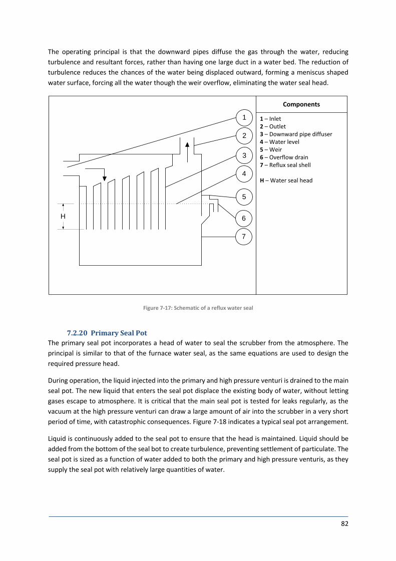
82
The operating principal is that the downward pipes diffuse the gas through the water, reducing
turbulence and resultant forces, rather than having one large duct in a water bed. The reduction of
turbulence reduces the chances of the water being displaced outward, forming a meniscus shaped
water surface, forcing all the water though the weir overflow, eliminating the water seal head.
Components
1 – Inlet2 – Outlet3 – Downward pipe diffuser4 – Water level5 – Weir6 – Overflow drain7 – Reflux seal shell
H – Water seal head
1
2
3
4
6
7
5
H
Figure 7-17: Schematic of a reflux water seal
7.2.20 Primary Seal Pot
The primary seal pot incorporates a head of water to seal the scrubber from the atmosphere. The
principal is similar to that of the furnace water seal, as the same equations are used to design the
required pressure head.
During operation, the liquid injected into the primary and high pressure venturi is drained to the main
seal pot. The new liquid that enters the seal pot displace the existing body of water, without letting
gases escape to atmosphere. It is critical that the main seal pot is tested for leaks regularly, as the
vacuum at the high pressure venturi can draw a large amount of air into the scrubber in a very short
period of time, with catastrophic consequences. Figure 7-18 indicates a typical seal pot arrangement.
Liquid is continuously added to the seal pot to ensure that the head is maintained. Liquid should be
added from the bottom of the seal bot to create turbulence, preventing settlement of particulate. The
seal pot is sized as a function of water added to both the primary and high pressure venturis, as they
supply the seal pot with relatively large quantities of water.

83
Components
1 – Seal pot shell2 – Inlet pipe3 – Overflow4 – Water body
H – Water seal head
1
2
3
4
H
Figure 7-18: Schematic of a seal pot
7.2.21 Fan Seal Pot
The fan seal pot is based on the same principal as the main seal pot, however it is significantly smaller
as it does not need to handle a continuous flow of water. Each fan typically has its own dedicated seal
pot to assist with maintenance.
7.2.22 Clean Gas Flare Tip
Designed similarly to that of the raw gas, the clean gas flare tip makes use of the same features and
components described for that of the raw gas. There are, however, dissimilarities specifically the
diameter, as the volumetric flow rate is significantly less due to the temperature difference. Also, the
material is of a lower grade as it does not need to withstand high temperatures, however the serrated
tip is still made from a heat resistant material.
7.2.23 Emergency Water Tank
The emergency water tank is designed to hold enough water to fill the furnace water seal twice. It is
located directly above the water seal, so that the height difference allows a larger pressure for the
water to be injected.
In the event of an emergency where the water supply is cut off instantly, or all other safety
mechanisms fail, the emergency tank will discharge its payload into the furnace water seal. The tank’s
outlet pipe is fitted with a spring-loaded fail-open valve, i.e. it will open automatically if the
compressed air or electrical supply were to fail.

84
Post-Design Experimentation
8.1 Primary Venturi Temperature To determine the effectiveness of the primary venturi design the inlet and outlet temperatures need
to be compared with that of the actual readings. The inlet and outlet temperatures are sampled
continuously over a period of 60 hours with hourly intervals, which is sufficient data to evaluate the
forecasted conditions. The temperatures are plotted in Figure 8-1, indicating a summary of the process
methodology.
Figure 8-1: Comparison of the furnace and primary venturi temperatures
To ensure that the equations used in Section 7.2 the primary venturi outlet temperature needs to be
compared with the actual readings to determine an error. These values are indicated in table 8-1.
Table 8-1: Comparison of forecasted versus sampled temperatures
Temperature Comparison
Venturi Inlet
[C]
Outlet
Forecast
[C]
Outlet
Actual
[C]
Deviation
[C]
Average 315.70 41.60 44.50 2.90
Maximum 409.00 45.80 47.10 7.50
Minimum 243.40 37.10 34.80 0.30
Standard deviation 34.28 1.79 2.09 2.55

85
Figure 8-2: Comparison between the forecasted and sampled temperatures
The difference in forecasted and actual temperatures is plotted in Figure 8-2. This gives a graphical
representation of the error magnitude.
8.2 Overall Scrubber Collection Efficiency To ensure that the scrubber conforms to environmental legislation, isokinetic sampling needs to be
conducted annually. This ensures that the scrubber plant does not lose efficiency over the course of
its lifetime, and also for deviations in efficiency to be identified regularly for remediation.
Isokinetic sampling was conducted over a period of two days, and a verified total of six samples were
sent off for laboratory testing and evaluation. A comparison between the forecasted and actual
sampled results are indicated in table 8-2.
Table 8-2: Forecasted versus actual collection efficiency
Collection Efficiency Comparison
Legal Limit
[mg/Nm3]
Forecasted
Emissions
[mg/Nm3]
Actual
Emissions
[mg/Nm3]
Deviation
[mg/Nm3]
Sample 1 100.00 71.57 33.60 37.97
Sample 2 100.00 71.57 53.30 18.27
Sample 3 100.00 71.57 35.30 36.27
Sample 4 100.00 71.57 52.40 19.17
Sample 5 100.00 71.57 50.60 20.97
Sample 6 100.00 71.57 49.30 22.27

86
Budget When budgeting for a plant of this magnitude it is difficult to accurately predict a cost, as prices
constantly fluctuate. Also, items that have longer lead-time can affect the cost of those with a shorter
lead-time, as escalation can have a negative effect over the final cost. It is therefore critical to ensure
that budgeting is done over a short period of time, and that a detailed and accurate buy-in schedule
be generated. For the purpose of this study, only a bill of quantities will be drafted, as a cost per unit
will only be accurate at the time of evaluation.
9.1 Bill of Quantities A typical high-level bill of quantities incorporates a breakdown of the plant requirements, to
summarise the necessary financial components. Table 9-1 indicates the items required for the
execution of a turn-key wet venturi scrubber plant project. A cost is not indicated for the items, as a
comprehensive budget breakdown can be found in appendix 11.4.
Table 9-1: Summarised requirements for a wet venturi scrubber
Wet Venturi Scrubber Requirements
Description Cost
Engineering R 6 275 625.00
Ducting and Stack R 21 250 777.50
Emergency Stack Equipment R 2 857 470.00
Primary Venturi Equipment R 4 698 290.00
Scrubber Ducting R 518 450.00
High Pressure Venturi Equipment R 2 387 287.50
Reflux Water Seal R 3 236 250.00
Main Fan Trains R 46 667 340.00
Control and Isolation Dampers R 4 030 025.00
Flare Tip Systems R 8 357 108.00
Support Structures R 2 810 400.00
Total Cost R 103 089 023.00
9.2 Financial Costing Failure to comply with environmental guidelines can result in hefty penalties, which can have a
detrimental effect on business. Also, the Department of Environmental Affairs has the authority to
cease all production on a furnace that is non-compliant, over and above the penalties discussed in
section 2. The lack of production with the current overheads of a furnace can cause bankruptcy within
months, as labour legislation and customer demands still exist when a production license has been
revoked.
The implementation of a scrubber plant is beneficial to both the environment and the financial
wellbeing of a furnace production company. A financial viability model needs to be calculated to
ensure that the return on production outweighs the cost of operation, along with capital required to
conform to environmental legislation. Clean furnace off-gas can be used to generate power, to reduce
furnace power consumption by pre-heating the charged material, which also encourages the
implementation of an efficient scrubber system.

87
Although the majority of corporations rely on financial return to justify operation, we are obligated to
ensure the wellbeing of the environment. This is often a costly exercise with a significant capital outlay,
however the benefits are clearly justified when considering what the human race stands to lose.
Conclusion Upon completion of the scrubber design the engineering, procurement and construction phases can
commence, followed by commissioning and start-up. The commissioning of a scrubber plant is a
process that requires patience and diligence. The hazardous nature of the furnace off-gas requires
that all safety aspects are met, along with a certified commissioning procedure.
10.1 Commissioning Procedure To commission a scrubber plant a step-by-step procedure needs to be followed, and each item is to
be verified by at least two persons. This reduces the possibility of errors, which can have catastrophic
consequences.
Table 10-1: Commissioning procedure for a wet venturi scrubber plant
Step Procedure Description
1 Pressure
testing
Conduct a pressure test on the system by applying compresses air,
approximately 1.25 times the operating pressure of the plant. This will
ensure that the water seal in the seal pots remain intact. A pressure gauge
is to be monitored for the duration of the test, so that a timeline can be
determine as to how long depressurization takes. The time duration is to
be in accordance with that of the specified test procedure, which varies
from each end-user.
2 Purging Once the pressure test has been conducted successfully, the scrubber
needs to be purged of all air, to eliminate the possibility of an explosion
within the system. This is done by displacing the air in the scrubber with
post-combusted furnace off-gas.
2.1 Inspection hatches on the furnace roof are opened to allow air to enter
the furnace.
2.2 One fan is then sped up to full speed and the liquid injection system on the
primary and high pressure venturis is opened to the required velocity. The
venturi throats are to remain in an open position until the purging is
complete.
2.3 The furnace water seal is then drained allowing the furnace gas to be
extracted. The air that is drawn into the furnace combusts above the
charged material, and the CO is converted into CO2.
2.4 Purging is to continue until the oxygen level on the gas analysers returns
an acceptable value.
2.5 Purging has thus been completed, and the furnace inspection hatches can
be closed. The scrubber plant with then continue to extract pure furnace
off-gas, and is to be considered a hazardous system.
3 Start-Up When one fan is running at full speed, the volumetric flow rate is the same
as if all three fans were running, as a fan is a constant volume displacing

88
component, and the total pressure is increases when more than one fan is
in series.
3.1 One fan cannot overcome the pressure drop of both venturi throats at
their operating position. Therefore their positions remain open as during
the purging process.
3.2 The second and third fan are then started up to full speed, while the
second and third fan are then started up to full speed, while the flow
control damper remains only slightly open and the furnace pressure
control damper fully open. This will allow the majority of gas to circulate,
rather than being discharged through the stack.
3.3 Once all three fans are running full speed, the furnace pressure control
damper needs to be set to an automatic controller, and the same for the
flow control damper.
3.4 The system will then proceed to extract all the gas from the furnace at a
constant flow rate, however the particulate elimination will only increase
once the venturis are set to their operating positions.
3.5 Both the primary and high pressure venturis are set to their operating
positions.
4 Control The system is very forgiving in a dynamic application, as the controllers will
compensate for any changes in the process parameters.
10.2 Evaluation of Post-Design Results To determine whether the design is successful, the forecasted calculated results needs to be
compared with the actual operating parameters.
10.2.1 Primary Venturi Temperatures
The forecasted average temperature difference across the primary venturi was calculated to be
274.1C, resulting in an average outlet temperature of 41.6C. For this forecast in temperature
decrease to be verified, it was compared to a set of temperature readings taken of the same period.
Test results returned an average temperature difference across the primary venturi of 271.2C, which
indicates a mean deviation of 2.90 when considering the series. This deviation is as a result of
variations in the system that cannot be predicted, however the control philosophy can mitigate the
majority of these changes effectively.
When considering the graphs in Section 9 it is clear the gas has reached saturation when calculated
with the method prescribed in Section 7. The verifications of the temperature samples with an
insignificant difference in saturation temperature deems the method to be successful and highly
accurate for future designs.
10.3 Overall Scrubber Collection Efficiency When considering the legal requirement aspect of the design efficiency, it is important to ensure that
the limitations will never be exceeded. For verification of the overall collection efficiency of the
scrubber, the design efficiency needs to be compared with the results returned in Section 9.

89
Figure 10-1 indicates that the actual emissions of the scrubber is well below the required parameters.
The difference between the design and actual collection efficiency is determined by the reaction
within the furnace. The design parameters used were to remove a certain percentage of the lightest
present element, carbon, thus increasing the efficiency of the scrubber in the presence of other
particulate. This allows for a margin to be incorporated, as the worst case scenario would be if only
carbon was extracted in the gas stream. The scrubber design would, however, be able to cater for this
scenario and operating within the parameters set by legislation.
The y-axis in Figure 10-1 indicates a comparison of the emissions, which clearly shows that the actual
scrubber emissions are less than that of both the legal and design requirements. When considering
the collection efficiency in Section 9 it is clear that the required amount of particulate has been
removed from the gas stream when calculated with the method prescribed in Section 7. The increase
in collection efficiency verifies that the design method is accurate and successful, as well as
incorporating a margin for the dynamic characteristic of a furnace.
Figure 10-1: Comparison of the actual scrubber emissions versus the legal and design requirements
10.4 Closing Immeasurable parameters prevent designing a scrubber that can perform the required task by
adapting to the bare minimum for the required efficiencies. It is good engineering practice to design
for the worst cases, thereby incorporating a margin for error during standard operating parameters.
There is, however, a limit as to how much of a margin is added during the design phase, as each
addition increases the overall cost of the plant. A balance needs to be obtained between the minimum
design requirement and the longevity of the plant, based on financial implications.
When all these aspects are taken into account a true engineering challenge is presented, as it is an
easy task to design an object when not adhering to practical and financial requirements. When

90
systems are designed competitively in the industry it is critical to maintain an edge over the
competition by making continual improvements to designs, thus optimizing the plant. This is a costly
task, as the return on research and development is only marginal compared to new engineering
concepts.
This work is based on the research supported by the South African Research Chairs Initiative of the
Department of Science and Technology and National Research Foundation of South Africa (Coal
Research Chair Grant No. 86880, UID85643, Grant No. 85632). Any opinion, finding or conclusion or
recommendation expressed in this material is that of the author(s) and the NRF does not accept any
liability in this regard.

91
10. Bibliography Ahrens, C.D., 2005. Essentials of Meteorology, 4th ed., Thomson Brooks/Cole, 472p.
Antoine, C., 1888, “Vapour Pressure: a new relationship between pressure and temperature”,
transl. Comptes Rendus des Séances de l'Académie des Sciences, pp. 681 – 684, pp. 778 – 780, pp. 836
– 837.
Austin, J., Brimblecombe, P. & Sturges, W., 2002, Air Pollution Science for the 21st Century. Oxford:
Elsevier Science Ltd., 676p.
Benilov, M.S., 2008, Understanding and modelling plasma – electrode interaction in high-pressure arc
discharges: a review, J. Phys. D: Appl. Phys. 41, 30pp.
Boubel, R.W., Fox, D.L., Turner, D.B. & Stern, A.C., 1994, Fundamentals of Air Pollution, 3rd ed.,
California: Academic Press. 574p.
Boulet, B., Lalli, G. & Ajersch, M., 2003, Modelling and Control of an Electric Arc Furnace, Centre of
Intelligent Machines, McGill University, pp. 3060 – 3064.
Clapeyron, M.C., 1834, "Mémoire sur la puissance motrice de la chaleur". Journal de l'École
polytechnique, pp. 153 – 190.
Clausius, R., 1850, “On the motive power of heat and the laws which can be deduced therefrom
regarding the theory of heat”, transl., Poggendorff’s Annalen der Physick, pp. 500 – 524.
Cunningham, E., 1910, "On the velocity of steady fall of spherical particles through fluid medium",
Proc. Roy. Soc. A 83, 357p.
Duxbury, A.C., & Sverdrup, K.A., 2002, An Introduction to the World’s Oceans, 7th ed., McGraw-Hill
College, 544p.
Grosvenor W.M., 1907, Calculations for dryer design, Trans. AIChE, Vol. 1. pp. 184-202.
Halliday, D. & Resnick, R., 2013, Fundamentals of Physics, Wiley, 524p.
Hinds, William C., 1999, Aerosol Technology, 2nd ed., Wiley – Interscience, 504p.
Kumar De, A. & Kumar De, A., 2005, Environmental Studies (Revised 2nd Edition). New Delhi: New Age
International (P) Ltd., Publishers. 247p.
Lapple, C., 1951, Processes uses many collector types, Chemical Engineering, 58:144.
Leith, D., 1984, Cyclones, in Handbook of powder science and technology, edited by M.A. Fayed and L.
Otten (Van Nostrand Reinhold Co.).
Liu, D.H.F, 1997, Environmental Engineer's Handbook, 2nd ed., CRC Press, 1454p.
Marland, G., Boden, T.A. & Andres, R.J., 2007, Global, Regional and National CO2 Emissions, A
Compendium of Data on Global Change, Oak Ridge National Laboratory, USDE.

92
McNaught, A.D. & Wilkinson, A., 1997, Compendium of Chemical Terminology, 2nd ed., “the Gold
Book”, Blackwell Science Inc., 464p.
Peat, C., "ISS Orbit". Heavens-Above, viewed 23 September 2013 from http://www.heavens-
above.com
Peirce, J.J., Weiner, R.F. & Aarne Vesilind, P., 1998, Environmental Pollution and Control, 4th ed.,
Woburn: Butterworth-Heinemann. 395p.
Perrot, P., 1998, A to Z of Thermodynamics. Oxford University Press, 336p.
Perry, R.H. and Green, D.W., 2007, Perry's Chemical Engineers' Handbook, 8th ed., McGraw-Hill, 2400p.
Pidwirny, M., 2006. "The Layered Atmosphere". Fundamentals of Physical Geography, 2nd ed.
Poling, B.E., Prausnitz, J.M. & O’Connell, J.P., 2000, The Properties of Gases and Liquids, 5th ed.,
McGraw-Hill Professional, 768p.
Rogers, R.R. & Yau, M.K., 1989, A Short Course in Cloud Physics, 3rd ed., Pergamon Press, 16p.
Rudnick, S.N., Koehler, J.L.M., Martin, K.P., Leith, D. & Cooper, D.W., 1986, Particle Collection
Efficinecy in a Venturi Scrubber: Comparison of Experiments with Theory. Environ. Sci. Technol., Vol.
20, No. 3, 1986, pp. 237 – 242.
Saravanan, K., Ramachandran, S. & Baskar, R., 2005, Principles of Environmental Science &
Technology. New Delhi: New Age International (P) Ltd., Publishers. 193p.
Shepherd, C.B. and Lapple, C.E., 1939, Air Pollution Control: A Design Approach in Cyclones, 2nd Ed., C.
David Cooper and F.C. Alley, pp. 127 – 139, Illinois: Woveland Press Inc.
Schifftner, K.C., 2002, Air Pollution Control Equipment Selection Guide. Florida: CRC Press LLC. 209p.
Schifftner, K.C. & Hesketh, H., 1983, Wet Scrubbers, Ann Arbor, Mich.: Ann Arbor Science.
Schnelle, K.B. & Brown, C.A., 2000, Air Pollution Control Technology Handbook. Florida: CRC Press LLC.
359p.
Spellman, Frank R. and Whiting, Nancy E., 2004, Environmental Engineer's Mathematics Handbook,
CRC Press, 664p.
Stairmand, C.J., 1951, The design and performance of cyclone separators, Trnas. Instn. Chem. Engrs.
29:356.
Stern, A.C., Kaplan, K.J. and Bush, P.D., 1956, Cyclone dust collectors, New York: American Petroleum
Institute.
Swift, P., 1969, Dust controls in industry. Steam and Heating Engineer, 38:453.
Tangstad, M. and Olsen, S.E., 1995, 'The Ferromanganese Process - Material and Energy Balance', in
Tuset, Tveit and Page (eds.), INFACON 7, Trondheim, Norway, pp. 621-630.
Theodore, L., 2008, Air Pollution Control Equipment. New Jersey: John Wiley & Sons, Inc. 574p.

93
Thompson, M., 2005, The Molecule of the Month, Carbon Monoxide, Winchester College, UK, viewed
August 2014, from http://www.chm.bris.ac.uk
Vallero, D., 2008, Fundamentals of Air Pollution, 4th ed., Burlington: Academic Press. 942p.
Van der Linde, M. & Feris, L. 2010, Compendium of South African Legislation, 2nd ed., Pretoria:
University Law Press. 690p.
Vezolli, C.A. & Manzini, E., 2008, Design for Environmental Sustainability, Springer, 304p.
Wang, L.K., Pereira, N.C. & Hung, Y.T., 2004, Air Pollution Control Engineering. New Jersey: Humana
Press. 504p.
Wang, L.K., Pereira, N.C. & Hung, Y.T., 2005, Advanced Air and Noise Pollution Control. New Jersey:
Humana Press. 526p.
Weiner, R.F. & Matthews, R., 2003, Environmental Engineering, 4th ed., Burlington: Butterworth-
Heinemann. 484p.
World Meteorological Organisation, 2008. Guide to Meteorological Instruments and Methods of
Observation. WMO-8. Seventh edition. Chapter 2, Measurement of Temperature.

94
Appendices
11.1 Particle Size Distribution Results at Different Furnace Loads Table 11-1: Particle size distribution results at 6.2MW
Date 16-Jan-13
Furnace Power [MW] 6.20
Total Particles 2499
Min Size 0.7
Max Size 24.3
Arithmetic Mean 4.1
Geometric Mean 3.6
From To Counts Percentage From To Counts Percentage
[μm] [μm] [%] [μm] [μm] [%]
0.0 0.2 0 0.00% 8.0 8.2 5 0.20%
0.2 0.4 0 0.00% 8.2 8.4 10 0.40%
0.4 0.6 0 0.00% 8.4 8.6 9 0.36%
0.6 0.8 21 0.84% 8.6 8.8 14 0.56%
0.8 1.0 2 0.08% 8.8 9.0 1 0.04%
1.0 1.2 34 1.36% 9.0 9.2 5 0.20%
1.2 1.4 48 1.92% 9.2 9.4 5 0.20%
1.4 1.6 112 4.48% 9.4 9.6 6 0.24%
1.6 1.8 14 0.56% 9.6 9.8 2 0.08%
1.8 2.0 90 3.60% 9.8 10.0 1 0.04%
2.0 2.2 49 1.96% 10 11 17 0.68%
2.2 2.4 77 3.08% 11 12 7 0.28%
2.4 2.6 47 1.88% 12 13 7 0.28%
2.6 2.8 187 7.48% 13 14 0 0.00%
2.8 3.0 134 5.36% 14 15 1 0.04%
3.0 3.2 254 10.16% 15 16 2 0.08%
3.2 3.4 56 2.24% 16 17 2 0.08%
3.4 3.6 45 1.80% 17 18 2 0.08%
3.6 3.8 50 2.00% 18 19 1 0.04%
3.8 4.0 229 9.16% 19 20 1 0.04%
4.0 4.2 134 5.36% 20 21 2 0.08%
4.2 4.4 40 1.60% 21 22 1 0.04%
4.4 4.6 152 6.08% 22 23 1 0.04%
4.6 4.8 39 1.56% 23 24 1 0.04%
4.8 5.0 81 3.24% 24 25 1 0.04%
5.0 5.2 20 0.80%
5.2 5.4 148 5.92%
5.4 5.6 16 0.64%
5.6 5.8 29 1.16%
5.8 6.0 55 2.20%
6.0 6.2 49 1.96%
6.2 6.4 4 0.16%
6.4 6.6 11 0.44%
6.6 6.8 76 3.04%
6.8 7.0 13 0.52%
7.0 7.2 5 0.20%
7.2 7.4 44 1.76%
7.4 7.6 0 0.00%
7.6 7.8 7 0.28%
7.8 8.0 23 0.92%

95
Table 11-2: Particle size distribution results at 9.0MW
Date 08-Feb-13
Furnace Power [MW] 9.00
Total Particles 2325
Min Size 0.7
Max Size 89.7
Arithmetic Mean 6
Geometric Mean 4.4
From To Counts Percentage From To Counts Percentage
[μm] [μm] [%] [μm] [μm] [%]
0.0 0.2 0 0.00% 8.0 8.2 5 0.22%
0.2 0.4 0 0.00% 8.2 8.4 23 0.99%
0.4 0.6 0 0.00% 8.4 8.6 11 0.47%
0.6 0.8 47 2.02% 8.6 8.8 29 1.25%
0.8 1.0 3 0.13% 8.8 9.0 1 0.04%
1.0 1.2 75 3.23% 9.0 9.2 10 0.43%
1.2 1.4 62 2.67% 9.2 9.4 13 0.56%
1.4 1.6 106 4.56% 9.4 9.6 21 0.90%
1.6 1.8 21 0.90% 9.6 9.8 5 0.22%
1.8 2.0 67 2.88% 9.8 10.0 8 0.34%
2.0 2.2 44 1.89% 10 11 62 2.67%
2.2 2.4 77 3.31% 11 12 41 1.76%
2.4 2.6 30 1.29% 12 13 46 1.98%
2.6 2.8 98 4.22% 13 14 35 1.51%
2.8 3.0 95 4.09% 14 15 25 1.08%
3.0 3.2 146 6.28% 15 16 16 0.69%
3.2 3.4 31 1.33% 16 17 11 0.47%
3.4 3.6 16 0.69% 17 18 15 0.65%
3.6 3.8 29 1.25% 18 19 11 0.47%
3.8 4.0 115 4.95% 19 20 9 0.39%
4.0 4.2 66 2.84% 20 21 7 0.30%
4.2 4.4 26 1.12% 21 22 10 0.43%
4.4 4.6 104 4.47% 22 23 7 0.30%
4.6 4.8 27 1.16% 23 24 2 0.09%
4.8 5.0 72 3.10% 24 25 5 0.22%
5.0 5.2 11 0.47% 25 26 4 0.17%
5.2 5.4 108 4.65% 26 27 4 0.17%
5.4 5.6 16 0.69% 27 28 3 0.13%
5.6 5.8 31 1.33% 28 29 4 0.17%
5.8 6.0 33 1.42% 29 30 3 0.13%
6.0 6.2 51 2.19% 30 31 4 0.17%
6.2 6.4 9 0.39% 31 32 1 0.04%
6.4 6.6 7 0.30% 32 33 3 0.13%
6.6 6.8 77 3.31% 33 34 2 0.09%
6.8 7.0 31 1.33% 34 35 2 0.09%
7.0 7.2 4 0.17% 35 36 2 0.09%
7.2 7.4 54 2.32% 36 37 1 0.04%
7.4 7.6 0 0.00% 37 38 1 0.04%
7.6 7.8 21 0.90% 38 39 2 0.09%
7.8 8.0 44 1.89% 39 89 6 0.26%
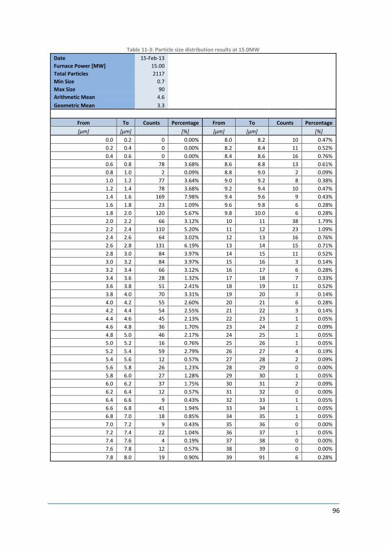
96
Table 11-3: Particle size distribution results at 15.0MW
Date 15-Feb-13
Furnace Power [MW] 15.00
Total Particles 2117
Min Size 0.7
Max Size 90
Arithmetic Mean 4.6
Geometric Mean 3.3
From To Counts Percentage From To Counts Percentage
[μm] [μm] [%] [μm] [μm] [%]
0.0 0.2 0 0.00% 8.0 8.2 10 0.47%
0.2 0.4 0 0.00% 8.2 8.4 11 0.52%
0.4 0.6 0 0.00% 8.4 8.6 16 0.76%
0.6 0.8 78 3.68% 8.6 8.8 13 0.61%
0.8 1.0 2 0.09% 8.8 9.0 2 0.09%
1.0 1.2 77 3.64% 9.0 9.2 8 0.38%
1.2 1.4 78 3.68% 9.2 9.4 10 0.47%
1.4 1.6 169 7.98% 9.4 9.6 9 0.43%
1.6 1.8 23 1.09% 9.6 9.8 6 0.28%
1.8 2.0 120 5.67% 9.8 10.0 6 0.28%
2.0 2.2 66 3.12% 10 11 38 1.79%
2.2 2.4 110 5.20% 11 12 23 1.09%
2.4 2.6 64 3.02% 12 13 16 0.76%
2.6 2.8 131 6.19% 13 14 15 0.71%
2.8 3.0 84 3.97% 14 15 11 0.52%
3.0 3.2 84 3.97% 15 16 3 0.14%
3.2 3.4 66 3.12% 16 17 6 0.28%
3.4 3.6 28 1.32% 17 18 7 0.33%
3.6 3.8 51 2.41% 18 19 11 0.52%
3.8 4.0 70 3.31% 19 20 3 0.14%
4.0 4.2 55 2.60% 20 21 6 0.28%
4.2 4.4 54 2.55% 21 22 3 0.14%
4.4 4.6 45 2.13% 22 23 1 0.05%
4.6 4.8 36 1.70% 23 24 2 0.09%
4.8 5.0 46 2.17% 24 25 1 0.05%
5.0 5.2 16 0.76% 25 26 1 0.05%
5.2 5.4 59 2.79% 26 27 4 0.19%
5.4 5.6 12 0.57% 27 28 2 0.09%
5.6 5.8 26 1.23% 28 29 0 0.00%
5.8 6.0 27 1.28% 29 30 1 0.05%
6.0 6.2 37 1.75% 30 31 2 0.09%
6.2 6.4 12 0.57% 31 32 0 0.00%
6.4 6.6 9 0.43% 32 33 1 0.05%
6.6 6.8 41 1.94% 33 34 1 0.05%
6.8 7.0 18 0.85% 34 35 1 0.05%
7.0 7.2 9 0.43% 35 36 0 0.00%
7.2 7.4 22 1.04% 36 37 1 0.05%
7.4 7.6 4 0.19% 37 38 0 0.00%
7.6 7.8 12 0.57% 38 39 0 0.00%
7.8 8.0 19 0.90% 39 91 6 0.28%

97
Table 11-4: Particle size distribution results at 30.0MW
Date 28-Feb-13
Furnace Power [MW] 30.00
Total Particles 2300
Min Size 0.7
Max Size 255
Arithmetic Mean 5
Geometric Mean 3.7
From To Counts Percentage From To Counts Percentage
[μm] [μm] [%] [μm] [μm] [%]
0.0 0.2 0 0.00% 8.0 8.2 7 0.30%
0.2 0.4 0 0.00% 8.2 8.4 15 0.65%
0.4 0.6 0 0.00% 8.4 8.6 12 0.52%
0.6 0.8 46 2.00% 8.6 8.8 19 0.83%
0.8 1.0 3 0.13% 8.8 9.0 6 0.26%
1.0 1.2 61 2.65% 9.0 9.2 10 0.43%
1.2 1.4 76 3.30% 9.2 9.4 10 0.43%
1.4 1.6 141 6.13% 9.4 9.6 20 0.87%
1.6 1.8 27 1.17% 9.6 9.8 7 0.30%
1.8 2.0 120 5.22% 9.8 56 9 0.39%
2.0 2.2 67 2.91% 10 38 28 1.22%
2.2 2.4 122 5.30% 11 19 19 0.83%
2.4 2.6 47 2.04% 12 25 12 0.52%
2.6 2.8 113 4.91% 13 15 15 0.65%
2.8 3.0 94 4.09% 14 13 16 0.70%
3.0 3.2 137 5.96% 15 17 10 0.43%
3.2 3.4 59 2.57% 16 10 9 0.39%
3.4 3.6 23 1.00% 17 12 9 0.39%
3.6 3.8 59 2.57% 18 4 7 0.30%
3.8 4.0 139 6.04% 19 4 8 0.35%
4.0 4.2 62 2.70% 20 6 8 0.35%
4.2 4.4 28 1.22% 21 6 6 0.26%
4.4 4.6 63 2.74% 22 2 9 0.39%
4.6 4.8 38 1.65% 23 4 9 0.39%
4.8 5.0 70 3.04% 24 2 3 0.13%
5.0 5.2 18 0.78% 25 3 6 0.26%
5.2 5.4 91 3.96% 26 2 5 0.22%
5.4 5.6 13 0.57% 27 2 1 0.04%
5.6 5.8 34 1.48% 28 3 2 0.09%
5.8 6.0 39 1.70% 29 0 1 0.04%
6.0 6.2 26 1.13% 30 4 1 0.04%
6.2 6.4 12 0.52% 31 0 4 0.17%
6.4 6.6 7 0.30% 32 2 2 0.09%
6.6 6.8 48 2.09% 33 1 0 0.00%
6.8 7.0 18 0.78% 34 0 1 0.04%
7.0 7.2 3 0.13% 35 1 2 0.09%
7.2 7.4 34 1.48% 36 0 0 0.00%
7.4 7.6 5 0.22% 37 1 1 0.04%
7.6 7.8 18 0.78% 38 1 1 0.04%
7.8 8.0 23 1.00% 39 251 1 0.04%

98
Table 11-5: Particle size distribution results at 42.0MW
Date 08-Mar-13
Furnace Power [MW] 42.00
Total Particles 2419
Min Size 0.7
Max Size 47.9
Arithmetic Mean 5
Geometric Mean 3.6
From To Counts Percentage From To Counts Percentage
[μm] [μm] [%] [μm] [μm] [%]
0.0 0.2 0.0 0.00% 8.0 8.2 6.0 0.25%
0.2 0.4 0.0 0.00% 8.2 8.4 17.0 0.70%
0.4 0.6 0.0 0.00% 8.4 8.6 11.0 0.45%
0.6 0.8 61.0 2.52% 8.6 8.8 16.0 0.66%
0.8 1.0 2.0 0.08% 8.8 9.0 0.0 0.00%
1.0 1.2 65.0 2.69% 9.0 9.2 6.0 0.25%
1.2 1.4 88.0 3.64% 9.2 9.4 10.0 0.41%
1.4 1.6 175.0 7.23% 9.4 9.6 19.0 0.79%
1.6 1.8 42.0 1.74% 9.6 9.8 10.0 0.41%
1.8 2.0 122 5.04% 9.8 56 12 0.50%
2.0 2.2 61 2.52% 10 38 32 1.32%
2.2 2.4 113 4.67% 11 19 27 1.12%
2.4 2.6 69 2.85% 12 25 16 0.66%
2.6 2.8 105 4.34% 13 15 14 0.58%
2.8 3.0 83 3.43% 14 13 7 0.29%
3.0 3.2 123 5.08% 15 17 16 0.66%
3.2 3.4 58 2.40% 16 10 13 0.54%
3.4 3.6 26 1.07% 17 12 7 0.29%
3.6 3.8 49 2.03% 18 4 12 0.50%
3.8 4.0 123 5.08% 19 4 8 0.33%
4.0 4.2 75 3.10% 20 6 9 0.37%
4.2 4.4 55 2.27% 21 6 9 0.37%
4.4 4.6 71 2.94% 22 2 4 0.17%
4.6 4.8 31 1.28% 23 4 2 0.08%
4.8 5.0 59 2.44% 24 2 3 0.12%
5.0 5.2 25 1.03% 25 3 2 0.08%
5.2 5.4 93 3.84% 26 2 1 0.04%
5.4 5.6 19 0.79% 27 2 1 0.04%
5.6 5.8 31 1.28% 28 3 4 0.17%
5.8 6.0 44 1.82% 29 0 3 0.12%
6.0 6.2 46 1.90% 30 4 0 0.00%
6.2 6.4 12 0.50% 31 0 2 0.08%
6.4 6.6 7 0.29% 32 2 1 0.04%
6.6 6.8 58 2.40% 33 1 2 0.08%
6.8 7.0 19 0.79% 34 0 2 0.08%
7.0 7.2 7 0.29% 35 1 1 0.04%
7.2 7.4 38 1.57% 36 0 1 0.04%
7.4 7.6 7 0.29% 37 1 2 0.08%
7.6 7.8 16 0.66% 38 1 1 0.04%
7.8 8.0 24 0.99% 39 48 8 0.33%
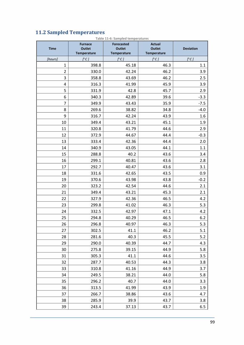
99
11.2 Sampled Temperatures Table 11-6: Sampled temperatures
Time Furnace Outlet
Temperature
Forecasted Outlet
Temperature
Actual Outlet
Temperature Deviation
[hours] [C ] [C ] [C ] [C ]
1 398.8 45.18 46.3 1.1
2 330.0 42.24 46.2 3.9
3 358.8 43.69 46.2 2.5
4 316.3 41.99 45.9 3.9
5 331.9 42.8 45.7 2.9
6 340.3 42.89 39.6 -3.3
7 349.9 43.43 35.9 -7.5
8 269.6 38.82 34.8 -4.0
9 316.7 42.24 43.9 1.6
10 349.4 43.21 45.1 1.9
11 320.8 41.79 44.6 2.9
12 372.9 44.67 44.4 -0.3
13 333.4 42.36 44.4 2.0
14 340.9 43.05 44.1 1.1
15 288.8 40.2 43.6 3.4
16 299.1 40.81 43.6 2.8
17 292.7 40.47 43.6 3.1
18 331.6 42.65 43.5 0.9
19 370.6 43.98 43.8 -0.2
20 323.2 42.54 44.6 2.1
21 349.4 43.21 45.3 2.1
22 327.9 42.36 46.5 4.2
23 299.8 41.02 46.3 5.3
24 332.5 42.97 47.1 4.2
25 294.8 40.29 46.5 6.2
26 296.8 40.97 46.3 5.3
27 302.5 41.1 46.2 5.1
28 281.6 40.3 45.5 5.2
29 290.0 40.39 44.7 4.3
30 275.8 39.15 44.9 5.8
31 305.3 41.1 44.6 3.5
32 287.7 40.53 44.3 3.8
33 310.8 41.16 44.9 3.7
34 249.5 38.21 44.0 5.8
35 296.2 40.7 44.0 3.3
36 313.5 41.99 43.9 1.9
37 266.7 38.86 43.6 4.7
38 285.9 39.9 43.7 3.8
39 243.4 37.13 43.7 6.5

100
40 272.3 38.98 43.1 4.1
41 314.4 41.48 43.0 1.5
42 353.8 43.8 44.2 0.4
43 409.0 45.79 45.1 -0.7
44 308.7 41.39 44.2 2.8
45 375.0 44.59 45.0 0.4
46 330.4 42.34 46.2 3.8
47 343.2 42.96 45.4 2.4
48 342.1 43.55 46.9 3.3
49 278.8 39.38 45.4 6.0
50 279.9 39.61 45.9 6.3
51 290.7 40.59 45.7 5.1
52 265.3 39.12 45.9 6.7
53 283.1 39.98 45.3 5.3
54 318.1 41.75 45.8 4.1
55 320.4 41.7 45.1 3.4
56 289.3 40.19 44.8 4.6
57 305.3 41.1 44.3 3.2
58 332.5 42.97 45.6 2.6
59 332.3 42.91 45.2 2.3
60 350.8 43.63 44.9 1.3

101
11.3 Emissions Sampling Isokinetic Test Results
[Page 1 of 2]
Sample No. 1 2 3
Start Time 00h00 13h05 15h05 10h27
End Time 00h00 13h16 15h15 10h37
Gas Temperature C 482 478 487
Barometric Pressure kPa 83.1 83.0 82.7
Duct Pressure Pa 97.2 147.0 130.5
Duct Pressure kPa (abs) 83.1 83.1 82.8
Nozzle Diameter mm 7.5 6.5 7.0
Sample Time min 12 10 8
Thimbles Used BL1 BL3 BL5
Total Duct Mass mg 1.6321 1.6403 1.0029
Velocity m/s 5.5 5.5 5.5
Gas Volume Flow Nm3/s 4.2 4.1 4.1
Gas Volume Flow Dry Nm3/s 4.1 4.1 4.1
Dust Concentration (wet) mg/Nm3 33.5 53.1 35.2
Dust Concentration (dry) mg/Nm3 33.6 53.3 35.3
Isokineticity % 93.8 95.4 95.6
ISO 9096, 12141 & 10155
ISO 9096:2003(E)
ISO #:825268/:2007-05-23 © ISO 2003
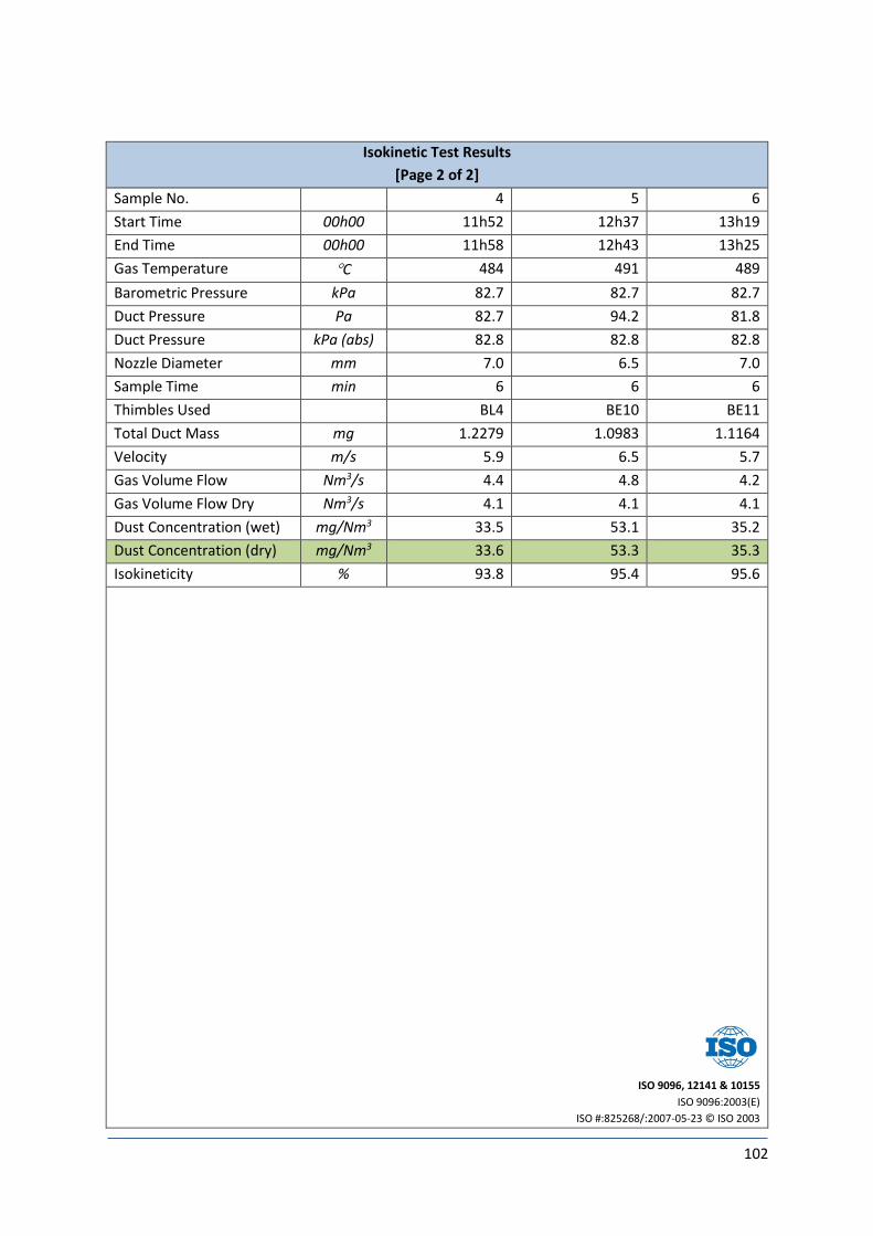
102
Isokinetic Test Results
[Page 2 of 2]
Sample No. 4 5 6
Start Time 00h00 11h52 12h37 13h19
End Time 00h00 11h58 12h43 13h25
Gas Temperature C 484 491 489
Barometric Pressure kPa 82.7 82.7 82.7
Duct Pressure Pa 82.7 94.2 81.8
Duct Pressure kPa (abs) 82.8 82.8 82.8
Nozzle Diameter mm 7.0 6.5 7.0
Sample Time min 6 6 6
Thimbles Used BL4 BE10 BE11
Total Duct Mass mg 1.2279 1.0983 1.1164
Velocity m/s 5.9 6.5 5.7
Gas Volume Flow Nm3/s 4.4 4.8 4.2
Gas Volume Flow Dry Nm3/s 4.1 4.1 4.1
Dust Concentration (wet) mg/Nm3 33.5 53.1 35.2
Dust Concentration (dry) mg/Nm3 33.6 53.3 35.3
Isokineticity % 93.8 95.4 95.6
ISO 9096, 12141 & 10155
ISO 9096:2003(E)
ISO #:825268/:2007-05-23 © ISO 2003

103
11.4 Budget Breakdown
1 Engineering
Description QTY Mass Hours Rate Cost
1.1 Mechanical Drawings 2300 R 675.00 R 1 552 500.00
1.2 Civil Drawings 85 R 675.00 R 57 375.00
1.3 Electrical and Instrumentation Drawings 375 R 675.00 R 253 125.00
1.4 Mechanical Engineering 550 R 625.00 R 343 750.00
1.5 Control and Instrumentation Engineering 350 R 550.00 R 192 500.00
1.6 Operating and Maintenance Manuals 200 R 900.00 R 180 000.00
1.7 Quality and Inspections 375 R 480.00 R 180 000.00
1.8 SHEQ 1350 R 450.00 R 607 500.00
1.9 Project Management 2750 R 1 050.00 R 2 887 500.00
1.10 Documentation Control 75 R 285.00 R 21 375.00
Sub-Total R 6 275 625.00
2 Ducting and Stack
Description QTY Mass Hours Rate Cost
2.1 Water Cooled Ducting 1 165000 R 85.00 R 14 025 000.00
2.2 Emergency Stack 1 78500 R 52.50 R 4 121 250.00
2.3 Support Steelwork 1 10800 R 48.00 R 518 400.00
2.4 Access Platforms 14 970 R 48.00 R 651 840.00
2.5 Painting 1 2750 R 52.50 R 144 375.00
2.6 Fasteners 5750 R 225.00 R 1 293 750.00
2.7 Ceramic Fibre Gaskets 985 R 22.50 R 22 162.50
2.8 Explosion Panels 80 R 5 925.00 R 474 000.00
Sub-Total R 21 250 777.50
3 Emergency Stack Equipment
Description QTY Mass Hours Rate Cost
3.1 Rotary Water Seal 2 8750 R 52.50 R 918 750.00
3.2 Rotary Water Seal Actuator 2 R 45 000.00 R 90 000.00
3.3 Emergency Stack Pressure Relief Valve 2 5650 R 52.50 R 593 250.00
3.4 Vertical Collector 2 3250 R 52.50 R 341 250.00
3.5 Support Steelwork 6 1250 R 48.00 R 360 000.00
3.6 Access Platforms 4 885 R 48.00 R 169 920.00
3.7 Painting 1 980 R 225.00 R 220 500.00
3.8 Fasteners 900 R 32.00 R 28 800.00
3.9 Agitator Set 6 R 22 500.00 R 135 000.00
Sub-Total R 2 857 470.00
4 Primary Venturi Equipment
Description QTY Mass Hours Rate Cost
4.1 Purge Pipe 40 mm Sch 40 2 50 R 105.00 R 10 500.00
4.2 Purge Valve 4 5 R 720.00 R 14 400.00

104
4.3 Primary Venturi Sump 2 800 R 52.50 R 84 000.00
4.4 Seal Pot 2 300 R 52.50 R 31 500.00
4.5 Drain Valve NB 100 2 5 R 135 000.00 R 1 350 000.00
4.6 Primary Venturi Section 2 1750 R 122.00 R 427 000.00
4.7 Primary Venturi Throat Section 2 460 R 122.00 R 112 240.00
4.8 Primary Venturi Down Pipe 2 1600 R 52.50 R 168 000.00
4.9 Primary Venturi Chamber Banjo 2 2000 R 52.50 R 210 000.00
4.10 Primary Venturi Chamber MS 2 7150 R 52.50 R 750 750.00
4.11 Painting Down duct 2 20 R 337.50 R 13 500.00
4.12 Painting Seperator 2 150 R 225.00 R 67 500.00
4.13 Ceramic fibre 2 R 4 500.00 R 9 000.00
4.14 Damper Linkage 2 R 9 000.00 R 18 000.00
4.15 Pneumatic Actuator 2 0 R 45 000.00 R 90 000.00
4.16 Support Steelwork 2 1000 R 48.00 R 96 000.00
4.17 Platforms 2 8 R 6 000.00 R 96 000.00
4.18 Cat ladder 26 220 R 52.50 R 300 300.00
4.19 Emergency Seal Tank 2 2500 R 122.00 R 610 000.00
4.20 Float Valve NB 100 2 R 3 750.00 R 7 500.00
4.21 Valve NB100 2 R 2 685.00 R 5 370.00
4.22 Valve NB 250 2 R 22 500.00 R 45 000.00
4.23 Valve NB 150 4 R 1 875.00 R 7 500.00
4.24 Valve NB 65 4 R 1 650.00 R 6 600.00
4.25 Pinch Valve NB 250 2 R 26 350.00 R 52 700.00
4.26 Non-Return NB 250 2 R 27 300.00 R 54 600.00
4.27 Non-Return NB 150 2 R 15 150.00 R 30 300.00
4.28 Non-Return NB 65 2 R 2 415.00 R 4 830.00
4.29 Piping NB 250 40 R 52.50 R 2 100.00
4.30 Piping NB 200 40 R 52.50 R 2 100.00
4.31 Piping NB 150 100 R 52.50 R 5 250.00
4.32 Piping NB 65 100 R 52.50 R 5 250.00
4.33 Fasteners 500 R 12.00 R 6 000.00
4.34 Painting 20 R 225.00 R 4 500.00
Sub-Total R 4 698 290.00
5 Scrubber Ducting
Description QTY Mass Hours Rate Cost
5.1 Refractory duct support 1 5000 R 48.00 R 240 000.00
5.2 Reflux support 1 490 R 48.00 R 23 520.00
5.3 Fan outlet support 1 490 R 48.00 R 23 520.00
5.4 Fan inlet support 1 500 R 48.00 R 24 000.00
5.5 Road support 2 515 R 48.00 R 49 440.00
5.6 Raw gas floor support 4 216 R 48.00 R 41 472.00
5.7 Clean gas tie support 4 144 R 48.00 R 27 648.00
5.8 Platform support Raw Gas 2 4 R 5 250.00 R 42 000.00
5.9 Cat ladder to support Raw Gas 40 0 R 52.50 R 2 100.00
5.10 Platform support Clean Stack 1 4 R 5 250.00 R 21 000.00

105
5.11 Cat ladder to support Clean Stack 20 0 R 52.50 R 1 050.00
5.12 Painting 1 25 R 180.00 R 4 500.00
5.13 Fasteners 650 R 28.00 R 18 200.00
Sub-Total R 518 450.00
6 High Pressure Venturi Equipment
Description QTY Mass Hours Rate Cost
6.1 Venturi Inlet Section 2 485 R 52.50 R 50 925.00
6.2 Throat 2 220 R 52.50 R 23 100.00
6.3 Damper Linkage 2 35 R 9 000.00 R 630 000.00
6.4 Pneumatic Actuator 2 R 45 000.00 R 90 000.00
6.5 Wet Elbow Section 2 1120 R 52.50 R 117 600.00
6.6 Eliminator MS 2 9225 R 52.50 R 968 625.00
6.7 Painting Inlet section 2 15 R 225.00 R 6 750.00
6.8 Painting Throat 2 20 R 225.00 R 9 000.00
6.9 Painting Wet Elbow 2 20 R 225.00 R 9 000.00
6.10 Painting Separator 2 195 R 225.00 R 87 750.00
6.11 Valves NB 50 20 R 975.00 R 19 500.00
6.12 Valves NB 100 4 R 2 775.00 R 11 100.00
6.13 Piping NB 50 50 R 150.00 R 7 500.00
6.14 Piping NB 100 50 R 375.00 R 18 750.00
6.15 Seal Pot 2 850 R 52.50 R 89 250.00
6.16 Support Steelwork 2 1000 R 48.00 R 96 000.00
6.17 Walkways 4 0 R 6 000.00 R 24 000.00
6.18 Hand Railing 300 5 R 65.63 R 98 437.50
6.19 Fasteners 2500 R 12.00 R 30 000.00
Sub-Total R 2 387 287.50
7 Reflux Water Seal
Description QTY Mass Hours Rate Cost
7.1 Reflux Water Seal Tank 1 7000 R 52.50 R 367 500.00
7.2 Painting (External) 1 85 R 225.00 R 19 125.00
7.3 Panting (Internal) 1 102 R 300.00 R 30 600.00
7.4 Overflow Weir 1 150 R 52.50 R 7 875.00
7.5 Valves and Piping 1 200 R 52.50 R 10 500.00
7.6 Inlet Transition Duct 1 480 R 52.50 R 25 200.00
7.7 Outlet Transition Duct 1 250 R 52.50 R 13 125.00
Sub-Total R 3 236 250.00
8 Main Fan Trains
Description QTY Mass Hours Rate Cost
8.1 Main Fan 6 R 3 481 365.00 R 20 888 190.00
8.2 Main Fan Motor 6 R 1 125 000.00 R 6 750 000.00
8.3 VSD Drives 6 R 1 920 000.00 R 11 520 000.00

106
8.4 Noise Insulation 1 R 225 000.00 R 225 000.00
8.5 Crawl Beams 3 1050 R 48.00 R 151 200.00
8.6 Hoist 3 R 62 500.00 R 187 500.00
8.7 Painting 120 R 180.00 R 21 600.00
8.8 Drain Sump 2 600 R 52.50 R 63 000.00
8.9 Water Sprays 24 12 R 3 000.00 R 864 000.00
8.10 Purge Valve NB 40 4 2 R 675.00 R 5 400.00
8.11 Purge Piping 40 60 R 127.50 R 306 000.00
8.12 Seal Pot 304 SS 2 800 R 105.00 R 168 000.00
8.13 Float Valve 2 2 R 4 500.00 R 18 000.00
8.14 Valve NB 65 4 2 R 1 650.00 R 13 200.00
8.15 Piping NB 65 50 200 R 225.00 R 2 250 000.00
Sub-Total R 46 667 340.00
9 Control and Isolation Dampers
Description QTY Mass Hours Rate Cost
9.1 1250 Control Damper 1 450 R 1 425.00 R 641 250.00
9.2 1250 Control Damper Actuator 1 50 R 4 500.00 R 225 000.00
9.3 900 Control Damper 2 400 R 1 350.00 R 1 080 000.00
9.4 900 Control Damper Actuator 2 50 R 450.00 R 45 000.00
9.5 900 Isolation Goggle Valve 2 400 R 1 525.00 R 1 220 000.00
9.6 900 I/D Power Pack 2 75 R 525.00 R 78 750.00
9.7 1250 Isolation Goggle Valve 2 400 R 600.00 R 480 000.00
9.8 1250 I/D Power pack 2 75 R 690.00 R 103 500.00
9.9 Compensator 1350 4 75 R 165.00 R 49 500.00
9.10 Compensator 1250 4 75 R 150.00 R 45 000.00
9.11 Compensator 900 4 75 R 135.00 R 40 500.00
9.12 Gaskets 14 R 375.00 R 5 250.00
9.13 Fasteners 14 R 600.00 R 8 400.00
9.14 Painting 35 R 225.00 R 7 875.00
Sub-Total R 4 030 025.00
10 Flare Tip System
Description QTY Mass Hours Rate Cost
10.1 Cat-ladders 8 560 R 52.50 R 235 200.00
10.2 Platforms 8 800 R 48.00 R 307 200.00
10.3 Support Steel 3 2550 R 48.00 R 367 200.00
10.4 Raw Gas Flare & Ignition System 2 R 1 925 000.00 R 3 850 000.00
10.5 Clean Gas Flare & Ignition System 2 R 1 356 000.00 R 2 712 000.00
10.6 Cables 360 R 225.00 R 81 000.00
10.7 Shipping 1 R 682 000.00 R 682 000.00
10.8 Gaskets 9 R 1 500.00 R 13 500.00
10.9 Bolts 864 R 22.00 R 19 008.00
10.10 Painting 400 R 225.00 R 90 000.00
Sub-Total R 8 357 108.00

107
11 Support Structures
Description QTY Mass Hours Rate Cost
11.1 Primary Venturi support structure 2 12000 R 48.00 R 1 152 000.00
11.2 High Pressure Venturi Support Structure 2 11000 R 48.00 R 1 056 000.00
11.3 Reflux Support Structure 1 250 R 48.00 R 12 000.00
11.4 Explosion Platforms 6 750 R 48.00 R 216 000.00
11.5 Paint Primary Venturi Structure 2 420 R 225.00 R 189 000.00
11.6 Paint High Pressure Venturi Structure 2 385 R 225.00 R 173 250.00
11.7 Paint Explosion Platforms 6 9 R 225.00 R 12 150.00
Sub-Total R 2 810 400.00
12 Total Cost
Grand Total R 103 089 023.00