designing for system reliability

© 2005 Eaton Corporation. All rights reserved.

Designing for System Reliability

Dave Loucks, P.E.

Eaton Corporation

http://www.eaton.com/

ToFacility


To UPS To UPS

FromMain


From Emergency Bus From Distribution Bus


What Reliability Is Seen At The Load?

Utility UPS Breaker Load

For example, if power flows to load as below: Assume outage duration exceeds battery capacity


Series Components


99.9% 99.99% 99.99%

For example, if power flows to load as below: Assume outage duration exceeds battery capacity


Series Components For example, if power flows to load as below:

Assume outage duration exceeds battery capacity


99.9%(8.7 hr/yr)

99.99%(0.87 hr/yr)

99.99%(0.87 hr/yr)

x+

x+

==

99.88%(10.5 hr/yr)

Overall reliability is poorer than any component reliability





99.9%(8.7 hr/yr)PF* = 0.1%

99.99%(0.87 hr/yr)

0.01%

99.99%(0.87 hr/yr)

0.01%

x++

x++

===

99.88%(10.5 hr/yr)

0.12%

PF = (1 – Reliability) = 1 – R(t)

* PF = probability of failure



If outage duration less than battery capacity

UPS Breaker Load

99.99%(0.87 hr/yr)

0.01%

99.99%(0.87 hr/yr)

0.01%

x++

===

99.98%(1.74 hr/yr)

0.02%*PF =

Batteries Depleted 99.88% reliable Batteries Not Depleted 99.98% reliable


Parallel Components What if power flows to load like this:


Utility

UPS

StaticATS

Load

UPS


Parallel Components

Utility

UPS

StaticATS

Load

UPS99.9%

99.99%

99.99%

99.99%

?? %

What if power flows to load like this: Assume outage duration exceeds battery capacity


Parallel Components

Utility Load

99.9%

99.99%

99.99%

99.99%PF* = 0.1% PF(a or b)+ + = ?? %

?? %

UPS

StaticATS

UPS

0.01%

What if power flows to load like this: Assume outage duration exceeds battery capacity


Parallel Components

99.99%

99.99%PF(a or b) = 0.01 % x = 0.000001 %

99.99 %

UPSa

UPSb

0.01%

What if power flows to load like this: Solve each path independently

99.99%

99.99%

UPSa

UPSb

99.99 %

R(t) = 1 - PF(a or b) = 99.999999%


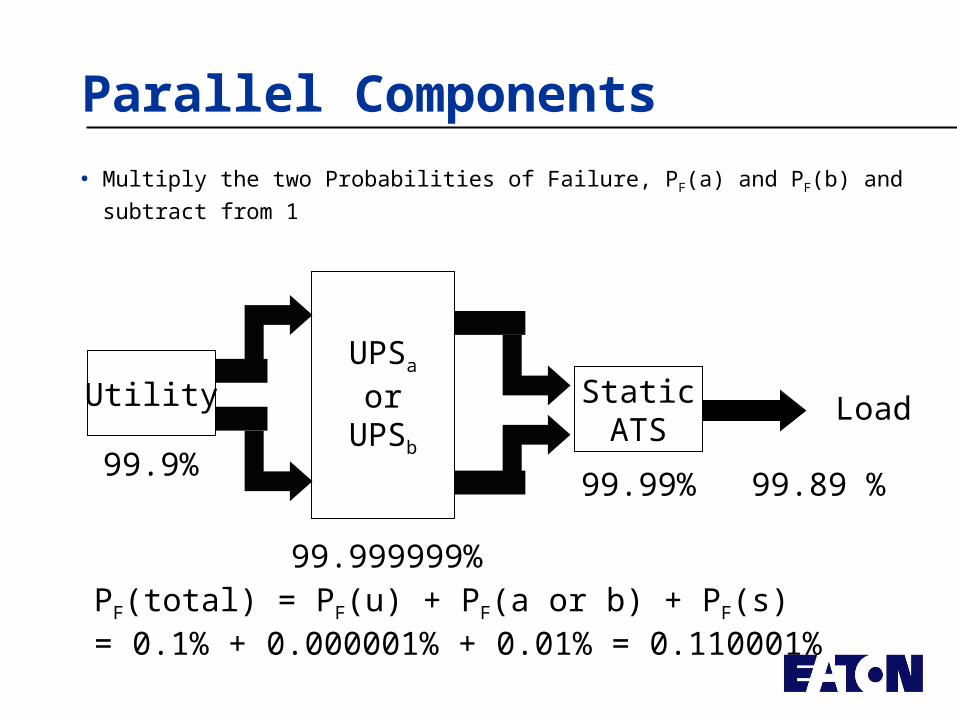
Parallel Components

Utility Load

99.9%99.99%

99.999999%

99.89 %

UPSa

orUPSb

StaticATS

Multiply the two Probabilities of Failure, PF(a) and PF(b) and subtract from 1

PF(total) = PF(u) + PF(a or b) + PF(s)= 0.1% + 0.000001% + 0.01% = 0.110001%


Parallel Components

Load

99.99%

99.999999%

99.99 %

UPSa

orUPSb

StaticATS

Multiply the two Probabilities of Failure, PF(a) and PF(b) and subtract from 1

PF(total) = PF(a or b) + PF(s)= 0.000001% + 0.01% = 0.010001%


Summary Table

Configuration Reliability

Single UPS system (long term outage) 99.88%

Single UPS system (short term outage) 99.98%

Redundant UPS system (long term outage) 99.89%

Redundant UPS system (short term outage) 99.99%

Comments?


Value AnalysisIs going from this:

Utility UPS Breaker

Utility

UPS

StaticATS

99.89%(only battery) 99.99%

UPS

99.88%(only battery) 99.89%

to this

worth it?

0.01%difference


Availability

Increase Mean Time Between Failures (MTBF) Decrease Mean Time To Repair (MTTR)

%100

MTTRMTBF

MTBFAi

i

i

A

AMTBFMTTR

)(

100


Relationship of MTBF and MTTR to Availability

0.65

0.7

0.75

0.8

0.85

0.9

0.95

1

0 10 20 30 40 50 60 70 80 90 100

MTTR (Hours)

Av

aila

bili

ty

1000 hrs800 hrs600 hrs

400 hrs

200 hrs

MTBF


95% Availability from Different MTBF/MTTR combinations

0.65

0.7

0.75

0.8

0.85

0.9

0.95

1

0 10 20 30 40 50 60 70 80 90 100

MTTR (Hours)

Av

aila

bili

ty

1000 hrs800 hrs600 hrs

400 hrs

200 hrs

MTBF

10.5 21.1 31.6 42.1 52.6


Breakeven Analysis Total Economic Value (TEV)

Simple Return (no time value of money)• TEVS = (Annual Value of Solution x Years of Life of Solution)

– Cost of Solution

Assume an outage > 0.1s costs $10000/yr

Assume cost of solution is $30000 Assume life of solution is 10 years


Breakeven Analysis

Since solution eliminates this potential 0.41 second outage, we “save” $10000 each year

Total Economic Value (TEV) Simple Return (no time value of money) TEVS = (Annual Value of Solution x Years of Life of

Solution) – Cost of Solution

TEVS = (($10000 x 1) x 10) – $100000

TEVS = $100000 - $30000 = $70000


Let’s Examine a More Complex System

52 52

Source 1 Source 2

What is the reliabilityat this point?

K K 52

Source 1


52

Source 299.9% 99.9%

99.99%

99.999%

99.99%

99.99%

99.99%

99.999%

99.9%

99.99%

99.999%

99.99%

99.9%

99.99%

99.999%

99.99%

99.99%

99.99%

99.999% 99.999%

Design 1 Design 2


Primary Selective

52 52

Source 1 Source 2


K K

99.9% 99.9%

99.99%

99.999%

99.99%

99.99%

99.99%

99.999%

Source 1 Source 2


99.999%

99.99%

99.99%

99.999%

.999 x .9999 = 99.89%

.999 x .9999 = 99.89%

99.89% 99.89%

Convert to

Design 1


Combine Reliabilities:Parallel Sources

52 52

Source 1 Source 2


K K

99.9% 99.9%

99.99%

99.999%

99.99%

99.99%

99.99%

99.999%

Source 1 or Source 2


99.999%

99.99%

99.99%

99.999%

PF1 x PF2 = PF both

PF both = 0.11% x 0.11%PF both = 0.0121%

R(t) = 1 – PF both

= 100% - 0.0121%= 99.99% PF1 = 0.0121%

R(t) = 99.99%

Design 1


Combine Reliabilities:Parallel Sources + Tx + Sec. Bkr.

52 52

Source 1 Source 2


K K

99.9% 99.9%

99.99%

99.999%

99.99%

99.99%

99.99%

99.999%



99.99%

99.999%

Rsource x Rtx x Rmb = R(t)= .9999 x .99999 x .9999

= .9998

R(t) = 99.98%

Design 1


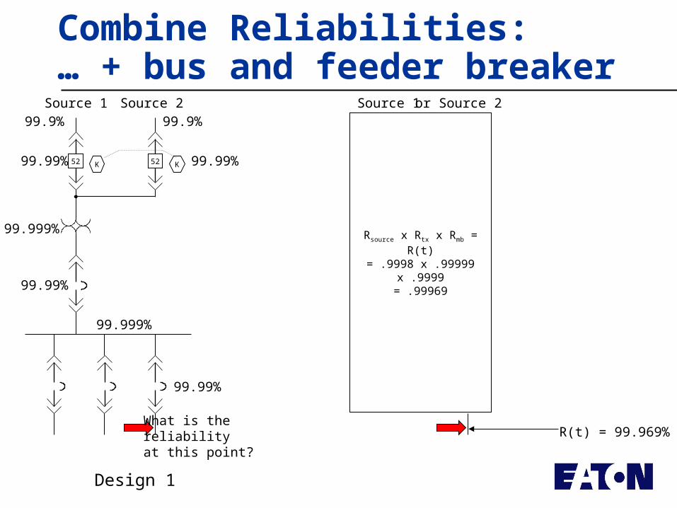
Combine Reliabilities:… + bus and feeder breaker

52 52

Source 1 Source 2


K K

99.9% 99.9%

99.99%

99.999%

99.99%

99.99%

99.99%

99.999%


Rsource x Rtx x Rmb = R(t)= .9998 x .99999 x .9999

= .99969

R(t) = 99.969%

Design 1


Secondary Selective

52

Source 1


52

Source 299.9%

99.99%

99.999%

99.99%

99.9%

99.99%

99.999%

99.99%

99.99%

99.999% 99.999%

99.99%

Design 2


Secondary Selective

52

Source 1


52

Source 299.9%

99.99%

99.999%

99.99%

99.9%

99.99%

99.999%

99.99%

99.99%

99.99%

99.999% 99.999%

Source 1 Source 2

99.99%

99.99%

99.999% 99.999%

R(t) = Rs x Rmb x Rtx x Rsb

= .999 x .9999 x .99999 x .9999

= .99879


= .999 x .9999 x .99999 x .9999

= .99879

R(t) = 99.88% 99.88%

Design 2


Secondary Selective

52

Source 1


52

Source 299.9%

99.99%

99.999%

99.99%

99.9%

99.99%

99.999%

99.99%

99.99%

99.99%

99.999% 99.999%

Source 1 Source 2

99.99%

99.99%

99.999% 99.999%


= .999 x .9999 x .99999 x .9999

= .99879


= .999 x .9999 x .99999 x .9999

= .99879

R(t) = 99.88%

Design 2


Secondary Selective

52

Source 1

52

Source 299.9%

99.99%

99.999%

99.99%

99.9%

99.99%

99.999%

99.99%

99.99%

99.999% 99.999%

Source 1 Source 2

Rtie = 99.99%

Rfdr =99.99%

Rbus1 = 99.999%

Rbus2 = 99.999%


= .999 x .9999 x .99999 x .9999

= .99879


= .999 x .9999 x .99999 x .9999

= .99879

Rs1 = 99.879%

Rpath1 = Rs1 x Rbus1 x Rtie x Rbus2 x Rfdr

Rpath1 = .99879 x .99999 x .9999 x .99999 x .9999 Rpath1 = .99857PF1 = 1 – Rpath1 = 1-.99857 = 0.00143 = 0.143%

Design 2


Secondary Selective

52

Source 1

52

Source 299.9%

99.99%

99.999%

99.99%

99.9%

99.99%

99.999%

99.99%

99.99%

99.999% 99.999%

Source 1 Source 2

Rfdr =99.99%

Rbus2 = 99.999%


= .999 x .9999 x .99999 x .9999

= .99879


= .999 x .9999 x .99999 x .9999

= .99879

Rpath2 = Rs2 x Rbus2 x Rfdr

Rpath2 = .99879 x .99999 x .9999Rpath2 = ..99868PF2 = 1 – Rpath2 = 1-.99868 = 0.00132 = 0.132%

Rs2 = 99.879%

Design 2


Secondary Selective

52

Source 1

52

Source 299.9%

99.99%

99.999%

99.99%

99.9%

99.99%

99.999%

99.99%

99.99%

99.999% 99.999%

Source 1 Source 2

R(t) = 1 – (PF1 x PF2)= 100% - (0.143% x 0.132%)

= 100% - (0.0189%)= 99.981%

R(t) = 99.981%

Design 2


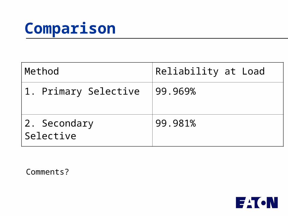
Comparison

Method Reliability at Load

1. Primary Selective 99.969%

2. Secondary Selective 99.981%

Comments?


Value Analysis

1. 99.97% x 8760 = failure once every 8757 hours

2. 99.98% x 8760 = failure once every 8758 hours Assuming 1 hour repair time, we will see two, 1-

hour outages after 8758 hours Meaning 1/8758 hours (0.411 seconds) expected outage

per year

As with UPS example, what is 0.411 seconds worth?

What is cost differential of higher reliability solution?


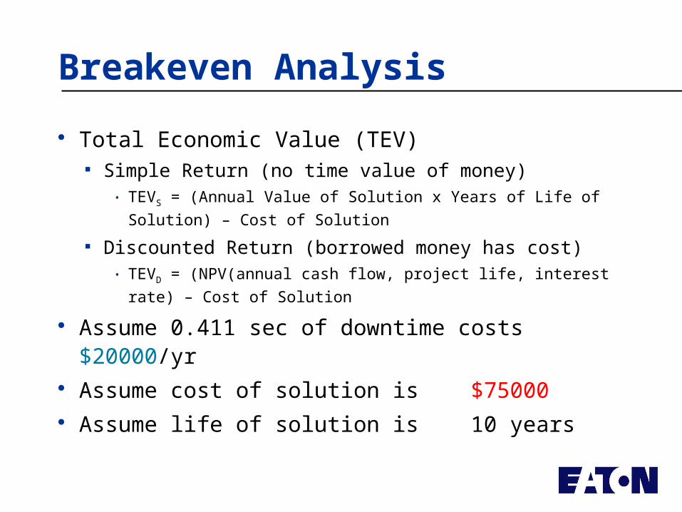
Breakeven Analysis

Total Economic Value (TEV) Simple Return (no time value of money)

• TEVS = (Annual Value of Solution x Years of Life of Solution) – Cost

of Solution

Discounted Return (borrowed money has cost)• TEVD = (NPV(annual cash flow, project life, interest rate) – Cost of

Solution

Assume 0.411 sec of downtime costs $20000/yr Assume cost of solution is $75000 Assume life of solution is 10 years


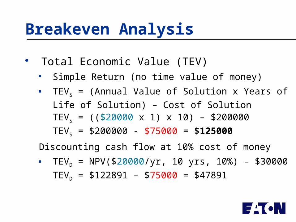
Breakeven Analysis


Solution) – Cost of SolutionTEVS = (($20000 x 1) x 10) – $200000

TEVS = $200000 - $75000 = $125000

Discounting cash flow at 10% cost of money TEVD = NPV($20000/yr, 10 yrs, 10%) – $30000

TEVD = $122891 – $75000 = $47891


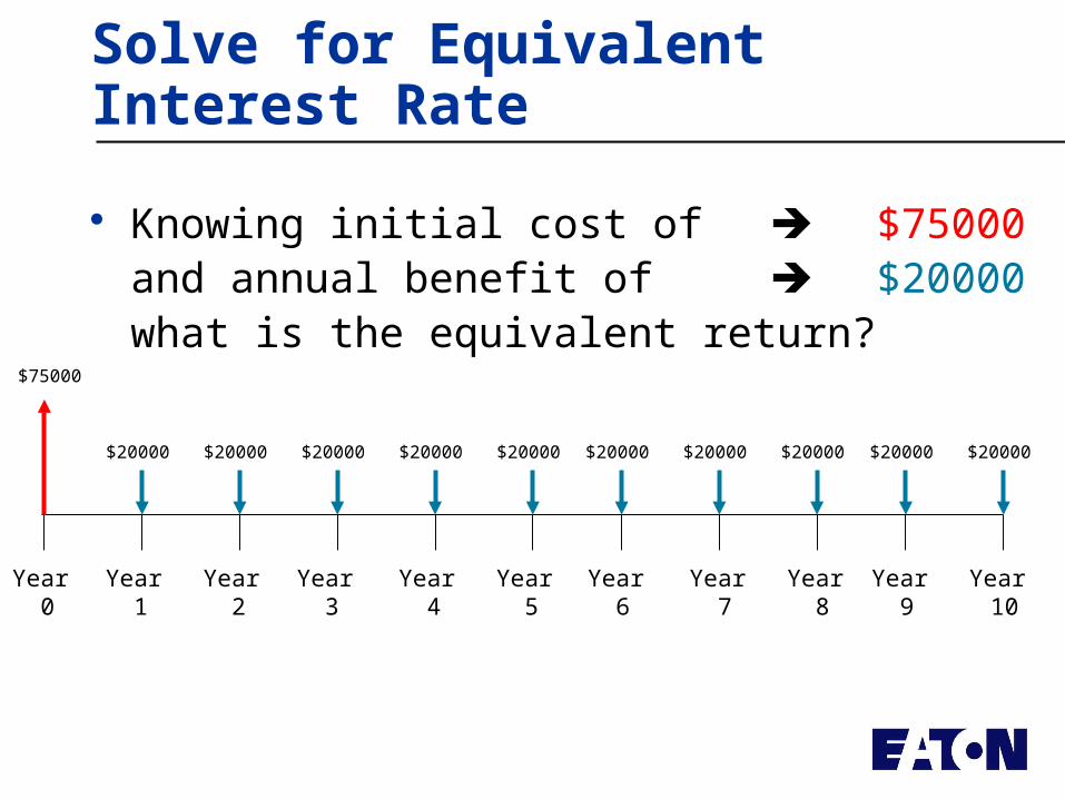
Solve for Equivalent Interest Rate

Knowing initial cost of $75000and annual benefit of $20000what is the equivalent return?

Year 1

Year 2

Year 3

Year 4

Year 5

Year 6

Year 7

Year 8

Year 9

Year 10

Year 0

$75000

$20000 $20000 $20000 $20000 $20000 $20000 $20000 $20000 $20000 $20000


Uniform Series Present Value

P – Present Value A – Annuity payment n – Number of periods

i – Interest per period

n =


Uniform Series Present Value Equations

But what if PV, A and n are known and i is unknown? Iterative calculation

n

n

ii

iAPV

1

11

11

1n

n

i

iiPVAor

P – Present Value A – Annuity payment n – Number of periods i – Interest per period


Uniform Series Present Value Equations

n

n

ii

iAPV

1

11

n i PV RS of Equation Comment

10 5% $75000 $154435 i too low

10 30% $75000 $61831 i too high

10 20% $75000 $83849 i too low

10 25% $75000 $71410 i too high

10 23.413% $75000 $75000 correct value


Breakeven Analysis


Solution) – Cost of SolutionTEVS = (($20000 x 1) x 10) – $200000

TEVS = $200000 - $75000 = $125000

Discounting cash flow at 10% cost of money TEVD = NPV($20000/yr, 10 yrs, 10%) – $30000

TEVD = $122891 – $75000 = $47891

IRR = 23.413% effective return


Reliability Tools

Eaton Spreadsheet Tools IEEE PCIC Reliability Calculator Commercially Available Tools Financial Tools (web calculators)


Web Based Financial Analysis

www.eatonelectrical.com search for “calculators” Choose “Life Extension

ROI Calculator”


Web Based Financial Analysis

Report provides financial data

Provides Internal Rate of Return

Use this to compare with other projects competing for same funds

Evaluates effects due to taxes, depreciation

Based on IEEE Gold Book data


Uncertainty – Heart of Probability

Probability had origins in gambling What are the odds that …

We defined mathematics resulted based on: Events

• What are the possible outcomes?

Probability• In the long run, what is the relative frequency that an event

will occur?

• “Random” events have an underlying probability function


Normal Distribution of Probabilities

From absolutely certain to absolutely impossible to everything in between

AbsolutelyCertain

100%

0%AbsolutelyImpossible

Most likely value


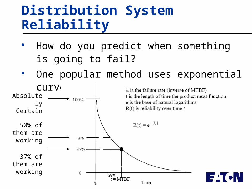
Distribution System Reliability How do you predict when something is going to

fail? One popular method uses exponential curve

AbsolutelyCertain

37% of them are working

50% of them are working

69%

50%


Mean Time Between Failures

The ‘mean time’ is not the 50-50 point (1/2 are working, 1/2 are not), rather…

When device life (t) equals MTBF (1/), then:

368011

.)(

eeetRt

MTBFt

The ‘mean time’ between failures when 37% devices are still operating


MTBF Review

Remember, MTBF doesn’t say that when the operating time equals the MTBF that 50% of the devices will still be operating, nor does it say that 0% of the devices will still be operating. It says 37% (e-1) of them will still be working.

Said another way; when present time of operation equals the mean (1/2 maximum life), the reliability is 37%


Exponential Probability

Assumes (1/MTBF) is constant with age For components that are not refurbished, we

know that isn’t true. Reliability decreases with age ( gets bigger)

However, for systems made up of many parts of varying ages and varying stages of refurbishment, exponential probability math works well.


Reliability versus MTBF

Assume at time = 0 Reliability equals 100% (you left it running)

At time > 0, Reliability is less than 100%

tMTBFt eetR

1

)(


Converting MTBF to Reliability

Unknown Reliability = ?

Known MTBF (40000 hrs) t (8760 hrs = 1 year)

tMTBFt eetR

1

)(

UPS

%.

)(

.

380

21908760

40000

1

1

ee

eetRt

MTBFt


Great, I’ve Found Problems, Now what?

You can certainly replace with newor…

If you catch it before it fails catastrophically, you can rebuild

Many old electrical devices can be rebuilt to like new condition


LV Refurbished Power Breakers LV Equipment Retrofit / “Roll-In” Replacements

510- Upgraded Trip

610- Display

810-KW-Comm-O/C

910-Harmonics

- (W) - C-H

- ITE - GE

- AC - FPE

- Siem - R-S


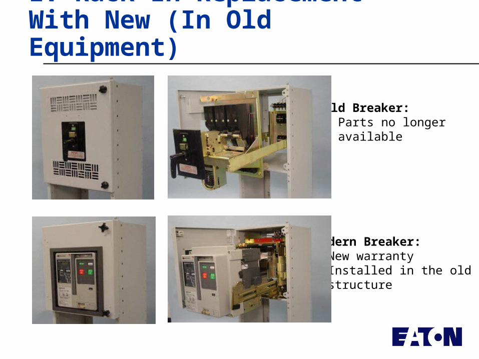
LV Rack-In Replacement With New (In Old Equipment)

Old Breaker:• Parts no longer available

Modern Breaker:• New warranty• Installed in the old structure


Motor Control Upgrades

MCC Bucket Retrofits- new breaker and starter

Breaker-to-Starter Conversions:- circuit breaker used to start motor- only good for 1000 or less operations- replace breaker with starter- now good for 1,000,000 operations

Continuous Partial Discharge Monitor


MV Vacuum Replacement•Vacuum replacement for Air Break in same space •Extensive Product Availability

• ANSI Qualified Designs• 158 Designs

• Non-Sliding Current Transfer• SURE CLOSE - Patented (MOC Switches)• 2-Year Warranty - Dedicated Service• Factory Trained Commissioning Engineers• Full Design & Production Certification• ANSI C37.59 Conversion Standard• ANSI C37.09 Breaker Standard• ANSI C37.20 Switchgear Standard• Design Test Certificate Available on Request


Can’t Buy a Spare? Class 1 Recondition Instead Receiving & Testing Complete Disassembly Detailed Inspection and

Cleaning New Parts OEM Re-assembly Testing Data-Base Tracking


Spot Network Upgrade

Network Protector Class 1

Recondition

Network Relay Upgrades...


InsulGard … “Predictive Relay”

MV Switchgear Applications:

* 15 Channel Inputs

* One (1) InsulGard for MV Switchgear & Transformer


designing for system reliability

Documents