development of a compositional model fully coupled …inside.mines.edu/~yxiong/xiong_thesis.pdf ·...
TRANSCRIPT

DEVELOPMENT OF A COMPOSITIONAL MODEL FULLY COUPLED
WITH GEOMECHANICS AND ITS APPLICATION TO TIGHT OIL
RESERVOIR SIMULATION
by
Yi Xiong

c© Copyright by Yi Xiong, 2015
All Rights Reserved
A thesis submitted to the Faculty and the Board of Trustees of the Colorado School
of Mines in partial fulfillment of the requirements for the degree of Doctor of Philosophy
(Petroleum Engineering).
Golden, Colorado
Date
Signed:Yi Xiong
Signed:Dr. Yu-Shu WuThesis Advisor
Golden, Colorado
Date
Signed:Dr. Erdal Ozkan
Professor and Interim Department HeadDepartment of Petroleum Engineering
ii

ABSTRACT
Tight oil reservoirs have received great attention in recent years as unconventional and
promising petroleum resources; they are reshaping the U.S. crude oil market due to their sub-
stantial production. However, fluid flow behaviors in tight oil reservoirs are not well studied
or understood due to the complexities in the physics involved. Specific characteristics of tight
oil reservoirs, such as nano-pore scale and strong stress-dependency result in complex porous
medium fluid flow behaviors. Recent field observations and laboratory experiments indicate
that large effects of pore confinement and rock compaction have non-negligible impacts on
the production performance of tight oil reservoirs. On the other hand, there are approxima-
tions or limitations for modeling tight oil reservoirs under the effects of pore confinement and
rock compaction with current reservoir simulation techniques. Thus this dissertation aims
to develop a compositional model coupled with geomechanics with capabilities to model and
understand the complex fluid flow behaviors of multiphase, multi-component fluids in tight
oil reservoirs.
MSFLOW COM (Multiphase Subsurface FLOW COMpositional model) has been de-
veloped with the capability to model the effects of pore confinement and rock compaction for
multiphase fluid flow in tight oil reservoirs. The pore confinement effect is represented by the
effect of capillary pressure on vapor-liquid equilibrium (VLE), and modeled with the VLE
calculation method in MSFLOW COM. The fully coupled geomechanical model is developed
from the linear elastic theory for a poro-elastic system and formulated in terms of the mean
stress. Rock compaction is then described using stress-dependent rock properties, especially
stress-dependent permeability. Thus MSFLOW COM has the capabilities to model the com-
plex fluid flow behaviors of tight oil reservoirs, fully coupled with geomechanics. In addition,
MSFLOW COM is validated against laboratory experimental data, analytical solutions and
results of a commercial simulator before conducting numerical studies.
iii
The numerical studies demonstrate the effect of capillary pressure on VLE, and further
on production performance. The significant effect of capillary pressure on VLE leads to the
suppression of bubble-point pressure and more light components dissolved in the oil phase.
Consequently it is observed that there is smaller gas saturations, larger mole fractions of
light components, and faster pressure decreasing at reservoir conditions; meanwhile less gas
and more oil are produced at surface.
The substantial decrease in reservoir pore pressure results in a large increase of effec-
tive stress, which induces the changes of rock properties and influences the production
performance. The stress-induced degradation of permeability undermines the production
performance, and the geomechanical effect on the permeability of natural fractures is mainly
responsible for the undermined production performance.
The reduction of pore size due to the geomechanical effect could increase the capillary
pressure, which enlarges the influence of capillarity on VLE and further suppresses bubble-
point pressure. On the other hand, the effect of capillary pressure on VLE influences the
fluid flow and therefore influences the effective stress through the flow-stress coupling process.
Thus the interaction between pore confinement and rock compaction can be modeled with
MSFLOW COM, and illustrated through numerical studies.
This research provides a three-dimensional numerical tool for accurately modeling porous
and fractured tight oil reservoirs. The developed simulator is able to assist scientists and
engineers to study and understand the complex multiphase, multi-component fluid flow
behaviors in tight oil reservoirs.
iv
TABLE OF CONTENTS
ABSTRACT . . . . . . . . . . . . . . . . . . . . . . . . . . . . . . . . . . . . . . . . . iii
LIST OF FIGURES . . . . . . . . . . . . . . . . . . . . . . . . . . . . . . . . . . . . . . x
LIST OF TABLES . . . . . . . . . . . . . . . . . . . . . . . . . . . . . . . . . . . . . . xiv
LIST OF SYMBOLS . . . . . . . . . . . . . . . . . . . . . . . . . . . . . . . . . . . . . xv
ACKNOWLEDGMENTS . . . . . . . . . . . . . . . . . . . . . . . . . . . . . . . . . . xix
CHAPTER 1 INTRODUCTION . . . . . . . . . . . . . . . . . . . . . . . . . . . . . . . 1
1.1 Overview of Tight Oil Reservoirs . . . . . . . . . . . . . . . . . . . . . . . . . . 1
1.2 Characteristics of Tight Oil Reservoirs . . . . . . . . . . . . . . . . . . . . . . . 3
1.2.1 Nano Pore Size and Ultra-low Permeability . . . . . . . . . . . . . . . . . 3
1.2.2 High Initial Reservoir Pressure . . . . . . . . . . . . . . . . . . . . . . . . 4
1.2.3 Large Fraction of Light Components . . . . . . . . . . . . . . . . . . . . 5
1.3 Complexities of Tight Oil Reservoir Modeling . . . . . . . . . . . . . . . . . . . 6
1.3.1 Pore Confinement Effect . . . . . . . . . . . . . . . . . . . . . . . . . . . 7
1.3.2 Rock Compaction Effect . . . . . . . . . . . . . . . . . . . . . . . . . . . 9
1.3.3 Interactions Between Pore Confinement and Rock Compaction . . . . . 10
1.4 Current Status and Limitation . . . . . . . . . . . . . . . . . . . . . . . . . . . 13
1.4.1 Coupled Geomechanical Effect . . . . . . . . . . . . . . . . . . . . . . . 13
1.4.1.1 Approximation in reservoir simulators . . . . . . . . . . . . . 14
1.4.1.2 Summary of Geomechanical Coupling Methods . . . . . . . . 15
1.4.2 Effect of Capillary Pressure on VLE . . . . . . . . . . . . . . . . . . . . 17
v

1.4.3 Current Limitations . . . . . . . . . . . . . . . . . . . . . . . . . . . . 18
1.5 Motivations and Objectives . . . . . . . . . . . . . . . . . . . . . . . . . . . . 19
1.5.1 Research Objectives and Tasks . . . . . . . . . . . . . . . . . . . . . . 20
1.5.2 Methodology . . . . . . . . . . . . . . . . . . . . . . . . . . . . . . . . 21
1.6 Thesis Organization . . . . . . . . . . . . . . . . . . . . . . . . . . . . . . . . . 21
CHAPTER 2 MATHEMATICAL MODEL . . . . . . . . . . . . . . . . . . . . . . . . 24
2.1 A General Compositional Model . . . . . . . . . . . . . . . . . . . . . . . . . . 24
2.2 Coupled Geomechanical Model . . . . . . . . . . . . . . . . . . . . . . . . . . . 25
2.3 Constitutive Relations . . . . . . . . . . . . . . . . . . . . . . . . . . . . . . . 28
2.3.1 Saturation and Volume Constraints . . . . . . . . . . . . . . . . . . . . 28
2.3.2 Composition Constrains . . . . . . . . . . . . . . . . . . . . . . . . . . 29
2.3.3 Capillary Pressure Functions . . . . . . . . . . . . . . . . . . . . . . . . 29
2.3.4 Relative Permeability Functions . . . . . . . . . . . . . . . . . . . . . . 30
2.4 Effects of Geomechanics . . . . . . . . . . . . . . . . . . . . . . . . . . . . . . 30
2.4.1 Effective Stress . . . . . . . . . . . . . . . . . . . . . . . . . . . . . . . 31
2.4.2 Porosity and Permeability . . . . . . . . . . . . . . . . . . . . . . . . . 31
2.4.3 Mass Conservation . . . . . . . . . . . . . . . . . . . . . . . . . . . . . 32
2.4.4 Capillary Pressure . . . . . . . . . . . . . . . . . . . . . . . . . . . . . 33
2.4.5 Relative Permeability . . . . . . . . . . . . . . . . . . . . . . . . . . . . 34
2.5 Summary and Discussions . . . . . . . . . . . . . . . . . . . . . . . . . . . . . 34
CHAPTER 3 VAPOR-LIQUID EQUILIBRIUM CALCULATION . . . . . . . . . . . 35
3.1 Phase Equilibrium Calculations . . . . . . . . . . . . . . . . . . . . . . . . . . 35
3.1.1 Theory of Phase Equilibrium Calculations . . . . . . . . . . . . . . . . 35
vi

3.1.2 Flow Chart of Phase Equilibrium Calculations . . . . . . . . . . . . . . 38
3.2 Saturation Pressure Calculation . . . . . . . . . . . . . . . . . . . . . . . . . . 38
3.3 Calculation Examples . . . . . . . . . . . . . . . . . . . . . . . . . . . . . . . . 40
3.4 Summary and Discussions . . . . . . . . . . . . . . . . . . . . . . . . . . . . . 44
CHAPTER 4 NUMERICAL METHODS AND SOLUTIONS . . . . . . . . . . . . . . 46
4.1 Discretized Governing Equations . . . . . . . . . . . . . . . . . . . . . . . . . 46
4.2 Boundary Conditions and Well Treatments . . . . . . . . . . . . . . . . . . . . 49
4.3 Numerical Solution Technique . . . . . . . . . . . . . . . . . . . . . . . . . . . 50
4.3.1 Residual Form . . . . . . . . . . . . . . . . . . . . . . . . . . . . . . . . 50
4.3.2 Degrees of Freedom and Primary Variables . . . . . . . . . . . . . . . . 50
4.3.3 Determination of Secondary Variables . . . . . . . . . . . . . . . . . . . 52
4.3.4 Solution Method . . . . . . . . . . . . . . . . . . . . . . . . . . . . . . 52
4.4 Program Implementation . . . . . . . . . . . . . . . . . . . . . . . . . . . . . . 54
4.5 Summary and Discussions . . . . . . . . . . . . . . . . . . . . . . . . . . . . . 58
CHAPTER 5 MODEL VALIDATION . . . . . . . . . . . . . . . . . . . . . . . . . . . 59
5.1 VLE Calculation . . . . . . . . . . . . . . . . . . . . . . . . . . . . . . . . . . 59
5.2 Black Oil Model . . . . . . . . . . . . . . . . . . . . . . . . . . . . . . . . . . . 62
5.2.1 Black Oil Model Simulation with Compositional Formulation . . . . . . 62
5.2.2 Buckley-Leverett Two-phase Vertical Flow . . . . . . . . . . . . . . . . 63
5.3 A General Compositional Model . . . . . . . . . . . . . . . . . . . . . . . . . . 65
5.4 One-dimensional Consolidation . . . . . . . . . . . . . . . . . . . . . . . . . . 70
5.5 Two-dimensional Compaction . . . . . . . . . . . . . . . . . . . . . . . . . . . 72
5.6 Summary and Discussions . . . . . . . . . . . . . . . . . . . . . . . . . . . . . 74
vii

CHAPTER 6 NUMERICAL STUDIES ON MATRIX ROCKS . . . . . . . . . . . . . 77
6.1 Simulation Setup . . . . . . . . . . . . . . . . . . . . . . . . . . . . . . . . . . 77
6.2 Simulation Results . . . . . . . . . . . . . . . . . . . . . . . . . . . . . . . . . 80
6.2.1 Above Saturation Pressure . . . . . . . . . . . . . . . . . . . . . . . . . 80
6.2.2 Below Saturation Pressure . . . . . . . . . . . . . . . . . . . . . . . . . 84
6.2.2.1 Effect of Capillary Pressure on VLE . . . . . . . . . . . . . . 85
6.2.2.2 Geomechanical Effect . . . . . . . . . . . . . . . . . . . . . . 93
6.2.3 Summary and Discussions . . . . . . . . . . . . . . . . . . . . . . . . . 97
CHAPTER 7 NUMERICAL STUDIES ON A FRACTURED RESERVOIR . . . . . . 99
7.1 A Fractured Reservoir With Double Porosity System . . . . . . . . . . . . . . 99
7.2 Geomechanical Effect . . . . . . . . . . . . . . . . . . . . . . . . . . . . . . . 102
7.2.1 Simulation Results . . . . . . . . . . . . . . . . . . . . . . . . . . . . 103
7.2.2 Sensitivity Analysis . . . . . . . . . . . . . . . . . . . . . . . . . . . . 106
7.3 Effect of Capillary Pressure . . . . . . . . . . . . . . . . . . . . . . . . . . . 108
7.3.1 Simulation Results . . . . . . . . . . . . . . . . . . . . . . . . . . . . 109
7.3.2 Sensitivity Analysis . . . . . . . . . . . . . . . . . . . . . . . . . . . . 119
7.4 Summary and Discussions . . . . . . . . . . . . . . . . . . . . . . . . . . . . 121
CHAPTER 8 CONCLUSIONS AND RECOMMENDATIONS . . . . . . . . . . . . . 123
8.1 Summary and Contributions . . . . . . . . . . . . . . . . . . . . . . . . . . . 123
8.2 Conclusions . . . . . . . . . . . . . . . . . . . . . . . . . . . . . . . . . . . . 124
8.3 Recommendations . . . . . . . . . . . . . . . . . . . . . . . . . . . . . . . . . 125
REFERENCES CITED . . . . . . . . . . . . . . . . . . . . . . . . . . . . . . . . . . 128
APPENDIX A - ANALYTICAL SOLUTIONS . . . . . . . . . . . . . . . . . . . . . . 137
viii

A.1 Buckley-Leverett Solution . . . . . . . . . . . . . . . . . . . . . . . . . . . . 137
A.2 1-D Consolidation Solution . . . . . . . . . . . . . . . . . . . . . . . . . . . . 138
A.3 2-D Compaction Solution . . . . . . . . . . . . . . . . . . . . . . . . . . . . . 138
APPENDIX B - FORMAT OF INPUT AND OUTPUT OF MSFLOW COM . . . . 140
B.1 Compositional Data Input - ’COMPS’ Section . . . . . . . . . . . . . . . . . 140
B.2 Geomechanical Input - ’ROCKS’ Section . . . . . . . . . . . . . . . . . . . . 142
B.3 Water Properties and Non-Darcy Coefficients - ’FLOWS’ Section . . . . . . 142
B.4 Other Computation options . . . . . . . . . . . . . . . . . . . . . . . . . . . 143
B.5 Number of Hydrocarbon Components . . . . . . . . . . . . . . . . . . . . . . 143
B.6 Output Files . . . . . . . . . . . . . . . . . . . . . . . . . . . . . . . . . . . . 144
ix

LIST OF FIGURES
Figure 1.1 (a) U.S. oil production by source, 1990-2040 . (b) U.S. tight oilproduction by geologic formation, 2008-2040 . . . . . . . . . . . . . . . . . . 2
Figure 1.2 Pore and pore-throat size spectrum (modified from Nelson, 2009). . . . . . 4
Figure 1.3 Pore-throat size distribution and nano-scale SEM image of Bakkenmatrix rock . . . . . . . . . . . . . . . . . . . . . . . . . . . . . . . . . . . . 5
Figure 1.4 Molar fraction of oil composition of Bakken oil (Light componentsaccounts for more than 50%). . . . . . . . . . . . . . . . . . . . . . . . . . . 6
Figure 1.5 Average API gravity of U.S. domestic and imported crude oil supplies,1990-2040 (◦API). . . . . . . . . . . . . . . . . . . . . . . . . . . . . . . . 7
Figure 1.6 Comparison of the contribution from capillary and surface forces on thebubble-point pressure for different oil samples . . . . . . . . . . . . . . . . . 8
Figure 1.7 Phase envelop of binary mixtures in 10 nm and 20 nm pores . . . . . . . . . 9
Figure 1.8 Bakken compaction table (constructed by Chu et al., 2012). . . . . . . . . 10
Figure 1.9 Pore radius reduction related to effective stress of Bakken reservoir . . . . 11
Figure 1.10 The interactions among fluid flow, rock compaction and poreconfinement. . . . . . . . . . . . . . . . . . . . . . . . . . . . . . . . . . . 12
Figure 1.11 Bakken history match with suppressed bubble point pressure andadjusted PVT properties . . . . . . . . . . . . . . . . . . . . . . . . . . . 18
Figure 3.1 Two phase equilibrium calculation including the effect of capillarypressure. . . . . . . . . . . . . . . . . . . . . . . . . . . . . . . . . . . . . 39
Figure 3.2 Saturation pressure calculation including the effect of capillary pressure. . 41
Figure 3.3 Saturation pressure (Bubble-point) of Eagle Ford oil. . . . . . . . . . . . . 43
Figure 3.4 Molar fraction of C1 + C2 in oil phase. . . . . . . . . . . . . . . . . . . . 44
Figure 3.5 Oil density and viscosity under capillarity effect. . . . . . . . . . . . . . 45
x

Figure 4.1 Space discretization and geometry data in the integral finite differencemethod . . . . . . . . . . . . . . . . . . . . . . . . . . . . . . . . . . . . . 46
Figure 4.2 Process for secondary variable calculation. . . . . . . . . . . . . . . . . . 53
Figure 4.3 Core modules and their relationships of MSFLOW COM. . . . . . . . . . 56
Figure 4.4 Simulation process of MSFLOW COM. . . . . . . . . . . . . . . . . . . . 57
Figure 5.1 Phase composition diagram at 500 psi and 160 ◦F. . . . . . . . . . . . . . 61
Figure 5.2 Phase composition diagram at 1500 psi and 160 ◦F. . . . . . . . . . . . . 61
Figure 5.3 Buckley-Leverett vertical flow problem and result. . . . . . . . . . . . . . 64
Figure 5.4 Compositional simulation example description. . . . . . . . . . . . . . . 66
Figure 5.5 Comparison of reservoir pressure and gas saturation of Node 1 and 100. . 67
Figure 5.6 Comparison of oil and gas saturation of Node 1 and 100. . . . . . . . . . 68
Figure 5.7 Comparison of accumulated production in moles. . . . . . . . . . . . . . . 68
Figure 5.8 Comparison of accumulated production at surface condition. . . . . . . . 69
Figure 5.9 One-dimensional consolidation processes under constant load. . . . . . . . 71
Figure 5.10 Pore pressure profile during drainage process under constant load. . . . . 72
Figure 5.11 Problem description of two-dimensional compaction. . . . . . . . . . . . . 73
Figure 5.12 Pore pressure evolution of central node (Mandel-Cryer effect). . . . . . . . 75
Figure 6.1 Simulation domain of Bakken matrix. . . . . . . . . . . . . . . . . . . . . 77
Figure 6.2 Effective stress evolution and induced change of permeability. . . . . . . 82
Figure 6.3 Comparison of oil production rate. . . . . . . . . . . . . . . . . . . . . . . 83
Figure 6.4 Comparison of pressure profile. . . . . . . . . . . . . . . . . . . . . . . . . 83
Figure 6.5 Comparison of accumulated oil and gas production between Run1 andRun2. . . . . . . . . . . . . . . . . . . . . . . . . . . . . . . . . . . . . . . 84
Figure 6.6 Gas saturation at three locations of Run2-1 and Run2-2. . . . . . . . . . 86
xi

Figure 6.7 Molar fraction of surface production. . . . . . . . . . . . . . . . . . . . . 87
Figure 6.8 Simulation results of molar fraction at x = 1.0 m. . . . . . . . . . . . . . 88
Figure 6.9 Simulation results of molar fraction at x = 15.0 m. . . . . . . . . . . . . . 88
Figure 6.10 Simulation results of molar fraction at x = 30.0 m. . . . . . . . . . . . . . 88
Figure 6.11 Simulation results of reservoir pressure at three locations. . . . . . . . . . 89
Figure 6.12 Reservoir pressure profile at the 10, 000th and 15, 000th day. . . . . . . . 89
Figure 6.13 Oil phase composition at reservoir condition. . . . . . . . . . . . . . . . . 90
Figure 6.14 Capillarity effect on oil density and viscosity under reservoir pressure. . . 91
Figure 6.15 Capillary pressure involved in VLE calculation. . . . . . . . . . . . . . . . 92
Figure 6.16 Comparison of accumulated production between Run2-1 and Run2-2. . . 92
Figure 6.17 Oil phase composition at reservoir condition. . . . . . . . . . . . . . . . . 93
Figure 6.18 Capillarity effect on oil density and viscosity under reservoir pressure. . . 94
Figure 6.19 Capillary pressure involved in VLE calculation. . . . . . . . . . . . . . . . 95
Figure 6.20 Simulation results of effective stress. . . . . . . . . . . . . . . . . . . . . . 96
Figure 6.21 Reservoir pressure, effective stress and permeability profile at end ofsimulation. . . . . . . . . . . . . . . . . . . . . . . . . . . . . . . . . . . . 96
Figure 6.22 Comparison of accumulated production. . . . . . . . . . . . . . . . . . . . 97
Figure 7.1 Schematic diagram of full reservoir: horizontal well, hydraulic fractures,and natural fractures. . . . . . . . . . . . . . . . . . . . . . . . . . . . . 100
Figure 7.2 Mesh system of hydraulic fractured reservoir. . . . . . . . . . . . . . . . 101
Figure 7.3 Fracture continuum: hydraulic fracture, macro-fracture andmicro-fracture. . . . . . . . . . . . . . . . . . . . . . . . . . . . . . . . . 101
Figure 7.4 Stress-induced permeability change outside SRV (location A) andwithin SRV (location B). . . . . . . . . . . . . . . . . . . . . . . . . . . 104
xii

Figure 7.5 Effective stress evolution outside SRV (location A) and within SRV(location B). . . . . . . . . . . . . . . . . . . . . . . . . . . . . . . . . . 105
Figure 7.6 Reservoir pressure evolution outside SRV (location A) and within SRV(location B). . . . . . . . . . . . . . . . . . . . . . . . . . . . . . . . . . 105
Figure 7.7 Permeability contour diagram at the end of simulation. . . . . . . . . . 106
Figure 7.8 Comparison of oil production due to geomechanical effect. . . . . . . . . 107
Figure 7.9 Comparison of reservoir pressure at the end of simulation. . . . . . . . . 107
Figure 7.10 Sensitivity analysis of geomechanical effects of different rocks. . . . . . . 108
Figure 7.11 Pressure contour diagram of Day 1 in fracture continuum. . . . . . . . . 109
Figure 7.12 Gas contour diagram of Day 1 in fracture continuum. . . . . . . . . . . 110
Figure 7.13 Gas saturation contour diagram after 10 years in both matrix andfracture continuum (left: without capillarity effect; right: withcapillarity effect; top: matrix system; bottom: fracture system). . . . . 111
Figure 7.14 Reservoir pressure contour diagram after 10 years in both matrix andfracture continuum (left: without capillarity effect; right: withcapillarity effect; top: matrix system; bottom: fracture system). . . . . 112
Figure 7.15 Gas saturation contour diagram after 60 years in both matrix andfracture continuum (left: without capillarity effect; right: withcapillarity effect; top: matrix system; bottom: fracture system). . . . . 113
Figure 7.16 Comparison of simulation results at location A (outside SRV). . . . . . 115
Figure 7.17 Comparison of simulation results at location B (within SRV). . . . . . . 116
Figure 7.18 Overall molar fraction after 60 years production. . . . . . . . . . . . . . 117
Figure 7.19 Molar fraction in oil phase after 60 years production. . . . . . . . . . . 118
Figure 7.20 Comparison of oil production. . . . . . . . . . . . . . . . . . . . . . . . 118
Figure 7.21 Comparison of gas production. . . . . . . . . . . . . . . . . . . . . . . . 119
Figure 7.22 Sensitivity study of capillarity effect on production performance. . . . . 120
Figure B.1 Snapshot of MSFLOW COM input file . . . . . . . . . . . . . . . . . . 141
xiii

LIST OF TABLES
Table 1.1 Summary of pressure gradient and depth of pay zones . . . . . . . . . . . . . 5
Table 1.2 Comparisons of different coupling approaches . . . . . . . . . . . . . . . . . 17
Table 3.1 Eagle Ford oil composition and component properties . . . . . . . . . . . . 42
Table 3.2 Eagle Ford oil binary interaction parameters . . . . . . . . . . . . . . . . . 43
Table 4.1 Primary variables and associated equations . . . . . . . . . . . . . . . . . 53
Table 5.1 Experimentally Determined Compositions . . . . . . . . . . . . . . . . . . 60
Table 5.2 Component properties used for validation of VLE calculation . . . . . . . . 60
Table 5.3 Rock and fluid properties of Buckley-Leverett vertical flow problem . . . . 64
Table 5.4 Rock and fluid properties used for compositional simulations . . . . . . . . 66
Table 5.5 Hydrocarbon component properties used for compositional simulations . . . 67
Table 5.6 Rock and fluid properties of 1-D consolidation problem . . . . . . . . . . . 71
Table 5.7 Rock and fluid properties of 2-D compaction problem . . . . . . . . . . . . 74
Table 6.1 Bakken oil composition and properties . . . . . . . . . . . . . . . . . . . . 78
Table 6.2 Bakken oil binary interaction parameters . . . . . . . . . . . . . . . . . . . 78
Table 6.3 Input parameters of Bakken matrix simulation . . . . . . . . . . . . . . . . 79
Table 6.4 Simulation run information for above bubble-point pressure . . . . . . . . . 81
Table 6.5 Simulation run information for below bubble point pressure . . . . . . . . . 85
Table 7.1 The hydraulic properties of different types of rocks . . . . . . . . . . . . 102
Table 7.2 The geomechanical properties of different types of rocks . . . . . . . . . 103
Table B.1 Additional output files by MSFLOW COM . . . . . . . . . . . . . . . . . 144
xiv

LIST OF SYMBOLS
Anm . . . . . . . . . . . . . . . . . . . . . . interface area of grid block n and m, m2 (ft2)
bK . . . . . . . . . . . . . . . . . . . . . . . . . . . . . . Klinkenberg coefficient, Pa (psi)
cb . . . . . . . . . . . . . . . . . . . . . . . . . . . . . . . bulk compressibility, Pa−1 (psi−1)
cp . . . . . . . . . . . . . . . . . . . . . . . . . . . . . . pore compressibility, Pa−1 (psi−1)
Deff,i . . . . . . . effective molecular diffusion coefficient of component i, m2/s (ft2/day)
Dig . . . . molecular diffusion coefficient of component i in bulk gas phase, m2/s (ft2/day)
dnm . . . . . . . . . . . . . . . . . . . . . . . distance between grid block n and m, m (ft)
Fb . . . . . . . . . . . . . . . . . . . . . . . . . . . . . . . . . . body force, Newton (lbf)
Fi . . . mass flux per unit volume of reservoir of component i, mol/m3/s (lbmol/ft3/day)
f oi . . . . . . . . . . . . . . . . . . . . . . . fugacity of component i in oil phase, Pa (psi)
f gi . . . . . . . . . . . . . . . . . . . . . . . fugacity of component i in gas phase, Pa (psi)
G . . . . . . . . . . . . . . . . . . . . . . . . . . . . . . . . . . . shear modulus, Pa (psi)
IFT . . . . . . . . . . . . . . . . . . . . . . . . . . . . interfacial tension, mN/m (lbf/in)
K . . . . . . . . . . . . . . . . . . . . . . . . . . . . . . . . . . . bulk modulus, Pa (psi)
Ki . . . . . . . . . . . . . . . . . . . . . . . . . . . . . . equilibrium ratio of component i
k . . . . . . . . . . . . . . . . . . . . . . . . . . . . . . . . absolute permeability, m2 (md)
knm+ 12
. . . . . . . . . . . . averaging permeability between grid blocks n and m, m2 (md)
krβ . . . . . . . . . . . . . . . . . . . . . . . . . . . . . . . relative permeability of phase β
Ni . . . . . . . . . . . . . . mass accumulation of component i, mol/m3/s (lbmol/ft3/day)
No, Ng . . . . . . . . . . . . . . . . . . . . . . . . moles of oil and gas phases, mol (lbmol)
xv

nc . . . . . . . . . . . . . . . . . . . . . . . . . total number of hydrocarbon components
nm . . . . . . . . . . . . . total number of all mass components (water plus hydrocarbon)
np . . . . . . . . . . . . . . . . . . . . . . . . . . . . . . . . . total number of fluid phases
no . . . . . . . . . . . . . . . mole fraction of oil phase in the whole hydrocarbon system
ng . . . . . . . . . . . . . . . mole fraction of gas phase in the whole hydrocarbon system
P . . . . . . . . . . . . . . . . . . . . . . . . . . . . . . . . . . . . . . . pressure, Pa (psi)
Pc . . . . . . . . . . . . . . . . . . . . . . . . . . . . . . . . . . critical pressure, Pa (psi)
Pcgo, Pcgw, Pcow . . . . . . . . . . . . . . . . . capillary pressure between phases, Pa (psi)
Psat . . . . . . . . . . . . . . . . oil saturation pressure (bubble-point pressure), Pa (psi)
qi . . . sink/source per unit volume of reservoir of component i, mol/m3/s (lbmol/ft3/day)
R . . . . . . . . . . . . . . . . . . . . . . ideal gas constant, JK−1mol−1 (ft3psiR−1lbmol−1)
r . . . . . . . . . . . . . . . . . . . . . . . . . . . . . . pore or pore-throat radius, m (in)
Sw, So, Sg . . . . . . . . . . . . . . . . . . . . . . . saturation of water, oil and gas phases
T . . . . . . . . . . . . . . . . . . . . . . . . . . . . . . . . . temperature, Kelvin (Rankin)
Tc . . . . . . . . . . . . . . . . . . . . . . . . . . . critical temperature, Kelvin (Rankin)
TM . . . . . . . . . . . . . . . . . . . . . . . . . . . . . . . . . transmissibility multiplier
t . . . . . . . . . . . . . . . . . . . . . . . . . . . . . . . . . . . . . . . time, second (day)
ui . . . . . . . . . . . . . . . . . . . . . . . . . . . . . displacement in direction i, m (ft)
Vb . . . . . . . . . . . . . . . . . . . . . . . . . . . . . . . . . Rock bulk volume, m3 (ft3)
Vp . . . . . . . . . . . . . . . . . . . . . . . . . . . . . . . . . Rock pore volume, m3 (ft3)
Vn . . . . . . . . . . . . . . . . . . . . . . . . . . . Rock volume of grid block n, m3 (ft3)
vw, vo, vg . . . . . . . . . . . . . . Darcy velocity of water, oil and gas phases, m/s (ft/day)
vc . . . . . . . . . . . . . . . . . . . . . . . . . . . . critical volume, m3/mol (ft3/lbmol)
xvi

x . . . . . . . . . . . . . . . . . . . . . . . . . . . . . . . . . . Vector of primary variables
xi . . . . . . . . . . . . . . . . . . . . . . . . . molar fraction in oil phase of component i
yi . . . . . . . . . . . . . . . . . . . . . . . . . molar fraction in gas phase of component i
Z . . . . . . . . . . . . . . . . . . . . . . . . . . . . . . . . . . . . . vertical depth, m (ft)
z . . . . . . . . . . . . . . . . . . . . . . . . . . . . . . . . . . . . . compressibility factor
zi . . . . . . . . . . . . . . . . . . . . . . . . . . . . . overall molar fraction of component i
α . . . . . . . . . . . . . . . . . . . . . . . . . . . . . . . . . . . . . . . . . Biot coefficient
β . . . . . . . . . . . . . . . . . linear thermal expansion coefficient, Kelvin−1 (Rankine−1)
Γn . . . . . . . . . . . . . . . . . . . . . . . . . . . surface area of grid blocks n, m2 (ft2)
γnm . . . . . . . . . . . . . . . transmissibility between grid blocks n and m, m3 (ft.md)
εv . . . . . . . . . . . . . . . . . . . . . . . . . . . . . . . . . . . . . . . volumetric strain
εij . . . . . . . . . . . . . . . . . . . . . . . . . . . . . . strain component in direction ij
ηn . . . . . . . . . . . . . . . . . . . . . . a set of neighboring grid blocks of grid block n
λ . . . . . . . . . . . . . . . . . . . . . . . . . . . . . . . . . . . Lames constant, Pa (psi)
µβ . . . . . . . . . . . . . . . . . . . . . . . . . . . . . . . . viscosity of phase β, Pa.s (cp)
µoi . . . . . . . . . . . . . . . . . chemical potential of component i in oil phase, Pa (psi)
µgi . . . . . . . . . . . . . . . . chemical potential of component i in gas phases, Pa (psi)
ν . . . . . . . . . . . . . . . . . . . . . . . . . . . . . . . . . . . . . . . . . Poisson’s ratio
ρw, ρo, ρg . . . . . . . . . . molar density of water, oil and gas phases, mol/m3 (lbmol/ft3)
σ, σmean, σ′
. . . . . . . . . . . . . . . . . . . stress, mean stress, effective stress, Pa (psi)
τ0 . . . . . . . . . . . . . . . . . . . . . . . . . . . . porous medium dependent tortuosity
τg . . . . . . . . . . . . . . . . . . . . . . . . . . . . gas saturation dependent tortuosity
Φoi . . . . . . . . . . . . . . . . . . . . . . fugacity coefficient of component i in oil phase
xvii

Φgi . . . . . . . . . . . . . . . . . . . . . fugacity coefficient of component i in gas phases
φ . . . . . . . . . . . . . . . . . . . . . . . . . . . . . . . . . . . . . . . . . . rock porosity
χi . . . . . . . . . . . . . . . . . . . . . . . . . . . . . . . Parachor value of component i
Ψβ . . . . . . . . . . . . . . . . . . . . . . . . . . . . . flow potential of phase β, Pa (psi)
ωi . . . . . . . . . . . . . . . . . . . . . . . . . . . . . . . acentric factor of component i
xviii

ACKNOWLEDGMENTS
First of all, I would like to express my deepest gratitude to my advisor, Dr. Yu-Shu Wu,
for his constant guidance, caring, patience and encouragement to me in the past few years.
I would never have been able to complete this dissertation without the research foundation
and platform he offers to me. He also provides me a perfect amount of freedom to pursue
the independent research work. His trust is one of the most important motivations for me
to finish this dissertation.
I also owe special thanks to my distinguished committee member: Dr. Tissa H. Illan-
gasekare, Dr. Xiaolong Yin, Dr. Azra N. Tutuncu, and Dr. Steve A. Sonnenberg. Dr.
Illangasekare provides me insightful comments and helpful suggestions since the first time I
met him. The excellent courses I took from Dr. Yin, Dr. Tutuncu, and Dr. Sonnenberg are
essentially valuable for completing this dissertation. I also would like to thank Dr. Philip H.
Winterfeld for his knowledge, expertise and patient help. I also truly appreciate the excellent
courses offered by Dr. Hossein Kazemi. His courses open the gate of reservoir simulation to
me and provide me essential and fundamental concepts.
I am grateful to the Energy Modeling Group (EMG) of petroleum engineering depart-
ment, directed by Dr. Yu-Shu Wu, for the financial support and wonderful team spirit. I also
appreciate the sponsors of EMG, especially Department of Energy (DoE), Foundation CMG,
and China National Petroleum Corporation (CNPC), for granting my research funding.
Last but not least, I would like to thank my wife, Yang. She is taking good care of
me and our child while pursuing her Ph.D. I could not complete my graduate study and
dissertation without her love, back and encouragement. My almost three-year-old daughter,
Liu-liu, makes my life of graduate study much more joyful. I also sincerely appreciate the
unconditional supports from my parents and parents-in-law.
xix

CHAPTER 1
INTRODUCTION
This chapter provides the background related to the key objectives and methodology
of this dissertation in five sections. Firstly the background of tight oil reservoirs and their
current production status are introduced. The second section focuses on the characteristics
of tight oil reservoirs, differentiating them from conventional reservoirs. These characteristics
lead to corresponding complexities and challenges for modeling and simulation of tight oil
reservoir, analyzed in the third section. The fourth section reviews the current efforts and
limits on modeling and simulation for tight oil reservoirs. Finally the motivations, and the
related objectives and methodology of this dissertation, are introduced in the last section.
1.1 Overview of Tight Oil Reservoirs
Tight oil reservoirs have received great attention in recent years as a type of uncon-
ventional resources because it is more economic than shale gas as well as technologies in
horizontal drilling and massive hydraulic-fracturing advance. The term tight oil, however,
is somewhat ambiguous in both industry and academia. According to US Energy Informa-
tion Administration (EIA, 2013a), “the term tight oil does not have a specific technical,
scientific, or geologic definition. Tight oil is an industry convention that generally refers to
oil produced from very-low-permeability shale, sandstone, and carbonate formations.” Al-
though the terms shale oil and tight oil are often used interchangeably in many contexts,
shale formations are only a subset of all low-permeability tight formations. Thus tight oil is
a more encompassing and accurate term with respect to the geologic formations producing
oil (EIA, 2013b) than shale oil. Being consistent with EIA terminology, in this dissertation a
tight oil reservoir refers to a petroleum reservoir generally with very-low-permeability rocks
(including shale plays) and an initial liquid-phase hydrocarbon fluid; and shale oil, a subset
of tight oil, only refers to the oil produced from shale formations.
1

Tight oil resources are enormous worldwide. EIA estimates the shale oil in-place and
technically recoverable shale oil resources of the world to 6,753 billion barrels and 335 billion
barrels, respectively (EIA, 2013b). Considering the fact that U.S. consumed 6.89 billion
barrels of petroleum products in 2013 (EIA, 2014b), tight oil resources could serve as the
primary energy supply for the next decades.
U.S. production of tight oil has increased dramatically in the past few years, from less
than 1 million barrels per day (MMbbl/d) in 2010 to more than 3 MMbbl/d in the second
half of 2013 (EIA, 2014a). The continued growth in tight oil production is projected in
Figure 1.1.
Figure 1.1: (a) U.S. oil production by source, 1990-2040 (EIA, 2014a).(b) U.S. tight oil production by geologic formation, 2008-2040 (EIA, 2013a).
Figure 1.1 (a) shows the oil production by source from 1990 and projected to 2040;
Figure 1.1 (b) shows the tight oil production by geologic formations from 2008 and projected
to 2040, both in million barrels per day. The projected U.S. total oil production increase
from 2008 and reach the peak about 2020 in Figure 1.1 (a) due to the sharp increase of lower
48 onshore. The growth of crude oil production in lower 48 onshore is primarily a result
of continued development of tight oil resources in Bakken, Eagle Ford, and Permian Basin
formations as shown in Figure 1.1 (b). In addition to above three main geologic sources,
2

other formations, including but not limited to the Austin Chalk, Niobrara, Monterey, and
Woodford formations accounts for remaining tight oil productions of U.S. (EIA, 2013a).
Tight oil reservoirs have been considered as the game changer for crude oil market. The
oil price has dropped by nearly half since August of 2014, and the increased oil supply due
to large production from tight oil reservoirs is one of the factors contributing to the dramatic
market change. In spite of some uncertainties of projections in Figure 1.1 due to substantial
change in oil price, it has been widely recognized that tight oil resources could be the primary
source for U.S. domestic oil production and energy supplies. EIA also claims a substantial
decrease of U.S. imported crude oil thanks to tight oil production (EIA, 2014a).
1.2 Characteristics of Tight Oil Reservoirs
A tight oil reservoir has the following characteristics differentiating itself from a con-
ventional petroleum reservoir. In addition, these characteristics lead to the corresponding
complexities and challenges for reservoir modeling and simulation described in Section 1.3.
1.2.1 Nano Pore Size and Ultra-low Permeability
Tight oil reservoir rocks have very small pore and pore-throat sizes with the scale of
nano-meters. For example, Kuila and Prasad (2011) pointed out that shale matrix has pre-
dominantly micro-pores with less than 2 nm diameter to meso-pores with 2-50 nm diameters.
Nelson (2009) claims that the normal range of pore and pore-throat size for the shale matrix
is from 5 to 50 nm, and publishes the pore-throat size spectrum for different types of rocks
shown in Figure 1.2. The range of pore and pore-throat sizes of matrix rocks for tight oil
reservoirs is ranged about from 5 - 100 nm and approximately marked in Figure 1.2.
The Middle Bakken interval, pay zone of Bakken tight oil reservoir, consists of tight
limestone and silt stones, with modal range of matrix pore sizes ranging from 10 nm to 50
nm (Chu et al., 2012; Nojabaei et al., 2013; Wang et al., 2013). This pore size distribution
is also confirmed by Honarpour et al. (2012), who compare the pore-throat size distribution
from mercury injection data on crushed vs. plug samples of Bakken rocks with results shown
3

Figure 1.2: Pore and pore-throat size spectrum (modified from Nelson, 2009).
in Figure 1.3 (a); Figure 1.3 (b) shows the pore network at nano and sub-nano scale of Bakken
matrix rock.
Such small pore size described above results in ultra-low matrix permeability of tight
oil reservoirs. Kurtoglu et al. (2014) tests the core plug permeability of Middle Bakken
sample using the steady-state method with a supercritical fluid. It is found that the low,
moderate and high permeability of Middle Bakken sample are 1.17×10⁻⁵ md, 6.27×10⁻⁴ md
and 1.25×10⁻³ md respectively.
1.2.2 High Initial Reservoir Pressure
The current economic producing tight oil reservoirs usually have very high initial reservoir
pressure. Over-pressure is one of key factors contributing to successful development of tight
oil reservoirs. For example, Bakken tight oil reservoir has the pressure gradient up to 0.75
psi/ft and initial reservoir pressure could reach as high as 7000 psi (Luneau et al., 2011) and
4

(a) Pore-throat radius distribution (b) nano-scale pore network
Figure 1.3: Pore-throat size distribution and nano-scale SEM image of Bakken matrix rock(Honarpour et al., 2012).
even higher. Similarly Eagle Ford formation has initial reservoir pressure of about 7500 psi
at 10500 feet TVD (true vertical depth) with a pressure gradient over 0.7 psi/ft (Deloitte,
2014). Wolfcamp shale in Permian basin also has pressure gradient up to 0.7 psi/ft and very
high initial reservoir pressure (Pioneer Natural Resource, 2013). Table 1.1 summarizes the
pressure gradient and the common depth of pay zones (Pioneer Natural Resource, 2013) of
U.S. major tight oil formations.
Table 1.1: Summary of pressure gradient and depth of pay zones
Reservoirs Pressure gradient TVD depth of pay zones(psi/ft) (feet)
Eagle Ford 0.60 - 0.80 7,500-11,000 (oil window)
Bakken 0.45 - 0.75 9,000-11,000
Permian Wolfcamp Shale 0.55 - 0.75 5,500-11,000
1.2.3 Large Fraction of Light Components
Another distinguished feature of tight oil reservoirs is that the initial oil composition has
a large molar fraction of light components. For example, the samples of Eagle Ford tight oil
with low, medium and high gas solubility have molar fractions of light components (C1 and
5

C2) as high as 35%, 50% and 63% (Orangi et al., 2011); the Middle Bakken tight oil also
has initial molar fraction of light components as high as 50% (Nojabaei et al., 2013; Wang
et al., 2013) shown in Figure 1.4.
Figure 1.4: Molar fraction of oil composition of Bakken oil (Light components accounts formore than 50%).
The large molar fraction of light components leads to a very high API value of produced
liquid. NRCan (Natural Resources Canada) calls tight oil as tight light oil (NRCan, 2014)
for this reason. Three major tight oil reservoirs in U.S., Bakken, Eagle Ford and Permian,
have most of produced liquid with API gravity above 40 ◦API (Deloitte, 2014; Honarpour
et al., 2012). Because of the production of light tight oil in U.S., EIA (2014a) projects API
increase for U.S. domestic oil production and decrease for imported crude oil as shown in
Figure 1.5, where the tight oil production explains the API increase of domestic oil and
decrease of imported oil from 2008 to 2015.
1.3 Complexities of Tight Oil Reservoir Modeling
The above characteristics of tight oil reservoirs lead to complex behaviors of subsurface
fluid flow. Two of the main complexities in flow behaviors, the effects of pore confinement
6

Figure 1.5: Average API gravity of U.S. domestic and imported crude oil supplies,1990-2040 (EIA, 2014a) (◦API).
and rock compaction, are discussed below.
1.3.1 Pore Confinement Effect
Section 1.2.1 describes the sizes of pore and pore-throat in tight oil reservoirs in nano-
meters. Such small pores lead to significant interfacial curvature and capillary pressure
between confined vapor and liquid phases. According to Zarragoicoechea and Kuz (2004),
there is a difference in thermodynamic phase behaviors for the fluids in confined and bulk
sizes. They point out that the phase behaviors and critical properties of the confined fluids
must be altered as a function of the ratio of the molecule size to the pore size. In the
other words, this pore confinement effect is non-negligible if the pore or pore-throat size is
comparable to the molecule size of the confined fluid.
Firincioglu et al. (2012) study the pore confinement effect on thermodynamic phase
behaviors by including capillary pressure and surface forces in vapor-liquid equilibrium (VLE)
calculation. The surface forces may contain structural, electrostatic and adsorbtive forces; for
practicality Firincioglu et al. (2012) only include van der Waals forces together with capillary
7

pressure in the VLE calculation. It is found that the contribution of the surface forces is very
small compared to the capillary force on the influence of phase behaviors. Figure 1.6 shows
the comparison of the contribution from capillary pressure and surface forces to influence on
the bubble point pressure. It shows that the contribution from surface forces is about a few
magnitudes smaller than that from capillary pressure; thus it is sufficient to represent the
pore confinement effect by including the capillary pressure in VLE calculation.
(a) (b) (c)
Figure 1.6: Comparison of the contribution from capillary and surface forces on thebubble-point pressure for different oil samples (Firincioglu et al., 2012).
Researchers have been investigating the impacts of capillary pressure on fluid properties
and phase behavior since the 1970s in oil and gas industry. It was found that the dew-point
and bubble-point pressure were same in the 30- to 40-US-mesh porous medium and in bulk
volume (Sigmund et al., 1973), and concluded that capillary effects on VLE is negligible for
conventional reservoirs. However, this assumption is not valid for tight oil reservoirs due
to nano-scale pore sizes. It is recognized that the bubble point pressures (oil saturation
pressure) of tight oil reservoirs are suppressed due to the capillary pressure. In other words,
the fluid bubble point pressure with same composition is lower in nano-pores than measured
in bulk size in PVT laboratory. Nojabaei et al. (2013) studies phase behaviors of several
binary mixtures in 20 nm and 10 nm pores with capillary pressure effect on VLE and shows
the differences in Figure 1.7.
Since there is a large fraction of light components in the oil composition discussed in Sec-
tion 1.2.3, the suppression on saturation pressure results in more light components remaining
8

(a) Phase envelop of binary mixtures in 10 nm pores (b) Phase envelop of binary mixtures in 20 nm pores
Figure 1.7: Phase envelop of binary mixtures in 10 nm and 20 nm pores (Nojabaei et al.,2013).
in oil phase instead of forming gas bubbles. Consequently the fluid properties, such as fluid
density and viscosity, are also affected, and it further complicates the fluid flow behaviors.
Thus it is necessary to improve or modify the conventional VLE calculation method for
capturing the effect of capillary pressure on phase behaviors for accurately modeling tight
oil reservoir.
1.3.2 Rock Compaction Effect
Since there is a very high initial pore pressure, and it is hard or even impossible to
maintain the initial pore pressure through fluid injection due to the ultra-low permeability,
the decrease of pore pressure is substantial during the production for tight oil reservoirs.
The large decrease of pore pressure, resulting in the increase of effective stress, further leads
to the rock compaction.
The rock properties of tight oil reservoirs thus have a strong stress-dependency due to the
influence of rock compaction. One of the major effects on rock properties is the degradation of
absolute permeability. Chu et al. (2012) construct the compaction tables related permeability
reduction factor and the change of effective stress for Bakken tight oil reservoir based on
9

laboratory measurements and history matches shown in Figure 1.8.
(a) Bakken compaction table based on lab data (b) Bakken compaction table based on history matches
Figure 1.8: Bakken compaction table (constructed by Chu et al., 2012).
In addition to Bakken tight oil reservoirs, other tight oil reservoirs also show strong
stress-dependent rock properties. For example, Orangi et al. (2011) performed a simulation
study for Eagle Ford tight oil reservoirs including the rock compaction effect and concludes
that the transmissibility could decrease by an order of magnitude due to degradation of the
fracture permeability.
Not only absolute permeability, other rock and fluid properties, such as porosity, relative
permeability(Lai and Miskimins, 2010) and capillary pressure etc., are also affected by rock
compaction and deformation. Therefore it is necessary to couple fluid flow and geomechanics
in order to model rock compaction effect on the production performance for tight oil reservoir.
1.3.3 Interactions Between Pore Confinement and Rock Compaction
The effects of pore confinement and rock compaction, discussed above, are two com-
plexities for modeling tight oil reservoirs. Another modeling complexity is the interactions
between pore confinement and rock compaction. On one hand, the rock compaction could
reduce the size of pores and pore-throats and further enlarge the pore confinement effect. For
example, Nojabaei et al. (2013) propose a pore radius reduction factor related to effective
stress for Bakken tight oil reservoir shown in Figure 1.9.
10

Figure 1.9: Pore radius reduction related to effective stress of Bakken reservoir (Nojabaeiet al., 2013).
On the other hand, the pore confinement effect, mainly the influence of capillary pressure
on VLE, suppresses the oil saturation pressure and correspondingly affects its fluid properties.
Consequently other reservoir properties, especially pore pressure, are also affected by pore
confinement effect during production. These influences resulting from pore confinement,
in turn, affect the reservoir effective stress. Thus the interactions among pore confinement
effect, rock compaction and fluid flow exist in tight oil reservoirs, and complicate the reservoir
modeling and simulation.
Figure 1.10 shows the interplays among fluid flow, rock compaction and pore confinement
in tight oil reservoirs. Each arrow in the figure represents the relationship between them
described by the numbers as follows.
1. Fluid flow effect on rock compaction: Fluid flow affects rock compaction through the
substantial decrease of pore pressure therefore the increase of effective stress;
2. Rock compaction effect on fluid flow: Rock compaction affects the fluid flow through
the stress-induced change on the rock properties, such as absolute permeability and
porosity etc.
11

Figure 1.10: The interactions among fluid flow, rock compaction and pore confinement.
3. Pore confinement effect on rock compaction: Pore confinement suppresses the satu-
ration pressure and influences the fluid properties, resulting in some effects on pore
pressure during production, which in turn affects the effective stress and rock com-
paction.
4. Rock compaction effect on pore confinement: The rock compaction results in the reduc-
tion of pore radius and the corresponding increase of capillary pressure, thus enlarges
the pore confinement effect.
5. Pore confinement effect on fluid flow: The pore confinement affects fluid flow behaviors
because it suppresses the oil saturation pressure and further affects the fluid properties,
such as fluid density and viscosity;
6. Fluid flow effect on pore confinement: The pore confinement, represented by the effect
of capillary pressure on VLE, is related to the capillary pressure, thus is affected by
the fluid flow, especially phase saturations.
Therefore it is complicated to model tight oil reservoirs because of the interplays among
fluid flow, pore confinement and rock compaction shown in Figure 1.10. In addition, the
12
multiple porous systems and the gas flow behaviors in tight reservoirs, such as Klinkenberg
effect (Klinkenberg, 1941) and molecular diffusion etc., add more complexities for tight oil
modeling. These complexities of fluid flow in multiple porous systems, and tight gas flow
behaviors have been thoroughly addressed in the literatures related to shale gas modeling
(Fakcharoenphol, 2013; Wu et al., 2014), thus not discussed in this dissertation.
1.4 Current Status and Limitation
The tight oil reservoir modeling involves the interactive processes among fluid flow, rock
compaction and pore confinement. The rock compaction modeling requires the coupling
between fluid flow and reservoir geomechanics; and the pore confinement effect could be
captured with a compositional model, where the VLE calculation includes the effect of
capillary pressure. This section reviews the status and existing limitations of current research
and engineering practices to solve above complexities of modeling tight oil reservoirs.
1.4.1 Coupled Geomechanical Effect
Stress-dependency of reservoir rock properties, especially porosity and permeability, have
been attracting intensive investigations through laboratory and modeling work for several
decades. Fatt and Davis (1952) reported the reduction in permeability with overburden
pressure back to 1950s. Dabbous et al. (1976, 1974) measured the air and water permeability
of a large number of coal samples at various overburden stress. Jones and Owens (1980)
performed laboratory study on low-permeability gas sands and claimed that the permeability
from routine core analysis could be more than 100 times greater than the permeability under
actual reservoir condition due to overburden stress. Ostensen (1986) studied the effect
of stress-dependent permeability on gas production and well testing. Davies and Davies
(2001) and McKee et al. (1988) investigated a large number of rock samples from different
formations and summarized several correlations between effective stress and rock porosity
and permeability. Rutqvist et al. (2002) applied the correlations between effective stress and
rock properties to the numerical simulations.
13

The laboratory investigations have been extended to shale and tight rocks in the past few
years because of the efforts on the development of unconventional resources. For example,
Cho et al. (2013) measured pressure-dependent natural-fracture permeability in shale and its
effect on shale-gas production; Mokhtari et al. (2013) studied stress-dependent permeability
anisotropy for Eagle Ford, Mancos, Green River, Bakken and Niobrara shales. Han et al.
(2013) investigated a nano-Darcy unconventional oil reservoir rock under true triaxial stress
conditions, and claimed that stress-dependency is more pronounced in low permeability rock
than in conventional reservoir rock.
The coupling between fluid flow and geomechanics is required to model rock compaction
effect on reservoir production performance. The remaining part of this section reviews the
approximation method used in conventional reservoir simulator to model geomechanical ef-
fect, and a variety of proposed coupling methods.
1.4.1.1 Approximation in reservoir simulators
The conventional (uncoupled) reservoir simulator does not generally incorporate stress-
dependent reservoir properties, but only approximates the changes of porosity as function
of pore pressure through pore volume compressibility defined as Equation (1.1).
cp = − 1
Vp
(∂Vp∂P
)(1.1)
where cp is the pore volume compressibility; Vp is the pore volume and P is pore pressure.
By the definition of porosity φ, the ratio of pore volume over bulk volume, Equation (1.1)
can be related to porosity as following:
cp = − 1
Vb
(∂Vb∂P
)+
1
φ
(∂φ
∂P
)= cb + cap (1.2)
where Vb is the bulk volume and cb is rock-bulk compressibility; cap = 1φ
(∂φ∂P
)is the ap-
proximation of pore volume compressibility obtained by ignoring cb, which is usually much
smaller than cp. For this reason, reservoir engineering literature usually considers pore vol-
14

ume compressibility same as rock compressibility(cR) or formation compressibility(cf ) by
ignoring cb (Ahmed, 2006; Ahmed and McKinney, 2011; Aziz and Settari, 1979; Craft et al.,
1991; Ertekin et al., 2001). In other words, pore volume compressibility has an approximated
definition as Equation (1.3) and it is usually used in reservoir engineering practices.
cp ≈ cap =1
φ
(∂φ
∂P
)(1.3)
Integrating above relation gives:
φ = φ0ecp(P−P0) ≈ φ0 [1 + cp (P − P0)] (1.4)
where P0 is the reference pore pressure at which the porosity is φ0. Equation (1.4) is used
to approximate the change of porosity as function of pore pressure with constant pore vol-
ume compressibility. It is one simplified method to capture rock deformation in conven-
tional(uncoupled) reservoir simulators (Aziz and Settari, 1979; Ertekin et al., 2001).
The above approximation to model the stress effect only includes the stress-induced
change on porosity. In recent years, the commercial petroleum reservoir simulators approxi-
mate stress-induced change on permeability by assigning a coefficient to transmissibility γ,
called transmissibility multiplier:
γ = TM(P ) ∗kmn+ 1
2Amn
dmn(1.5)
where TM is the transmissibility multiplier, which is a function of reservoir pore pressure
P .
1.4.1.2 Summary of Geomechanical Coupling Methods
The conventional simplification for rock deformation explained in previous section is not
sufficient for stress-sensitive reservoir simulations. A variety of methods for coupling fluid
flow and geomechanics have been proposed. (Dean et al., 2006; Gutierrez et al., 2001; Minkoff
et al., 2003; Settari and Walters, 2001; Tran et al., 2009). From loose to tight, there are
usually three types of coupling methods:
15
1. Explicit Coupling: For an explicit coupled method, the reservoir simulator performs
fluid flow calculations at each time step and the flow solutions are passed to geome-
chanical model at selected time step for stress calculations. This approach is also
called one-way coupling because only flow solutions are inputted for geomechanical
calculations while geomechanical solutions do not feedback to flow calculations.
2. Iterative Coupling: Fluid flow and geomechanics sub-systems are solved separately and
sequentially at each time step. Usually the fluid flow equation systems are solved first
and the solutions are passed to geomechanics system. The solution of geomechanics
equations then feeds back to fluid flow system until the total equation systems reach
convergence. This approach is a two-way coupling.
3. Fully Coupling: For a fully coupled method, the fluid flow and geomechanics variables
are solved simultaneously through one set of equation system. This is the most tight
coupling method.
Tran et al. (2009) proposed three aspects, accuracy, adaptability and running speed to
evaluate each coupling approach. Accuracy refers to how close the numerical results to the
real or benchmark solutions. Adaptability, in another word, flexibility, means how easy to
couple the existing or mature flow simulators and geomechanics simulators without large code
change or subsequent maintenance. Running speed is related to computational efficiency and
it is an important factor for practical full-field simulations.
Explicit coupling approach has very good adaptability and running speed because of
loose coupling between two independent simulators but has poor accuracy due to one-way
information transfer. Iterative coupling also has quite good adaptability but less running
speed than explicit coupling because the geomechanics computations are performed at each
time step instead selected time step in explicit coupling; but its two-way information trans-
fer gives better accuracy than explicit coupling approach. Fully coupling approach has the
best accuracy; but it requires much coding work for the coupling and does not run as fast
16

as the explicit method. Fully coupling is unconditionally stable compared to other cou-
pling approaches. Table 1.2 summarizes the advantages and disadvantages for each coupling
approach.
Table 1.2: Comparisons of different coupling approaches
Coupling Approaches Adaptability Running speed Accuracy
Explicit Coupling Good Good Poor
Iterative Coupling Fair not as good as explicit coupling Fair
Fully Coupling Poor not as good as explicit coupling Good
Table 1.2 is a general comparison for each coupling method and it may vary for specific
simulators. In general, the looser coupling method gives higher adaptability and running
speed but less accuracy, and vice versa.
1.4.2 Effect of Capillary Pressure on VLE
The pore confinement effect on tight oil reservoirs, can be represented as the effect of
capillary pressure on VLE based on the discussion in Section 1.3.1. It has been recognized
that the effect of capillary pressure on VLE is non-negligible for tight oil reservoir modeling.
Wang et al. (2014) performed experimental to study on the effect of pore size distribu-
tion on phase behaviors in nanopores, and found that the capillary pressure due to nano-
confinement increased the level of supersaturation and had a strong influence on the prop-
erties of produced fluids. In addition to experimental work, there also are several simulation
practices including the effect of capillary pressure on VLE.
For example, Nojabaei et al. (2013) incorporated the capillary pressure effects for Bakken
reservoir simulation with suppressed bubble-point pressure and adjusted PVT properties,
and found a better history match shown in Figure 1.11. In addition, Du and Chu (2012)
studied the PVT properties with capillary pressure effect on phase behaviors for reservoirs
with a variety of permeability and gas solubility.
17

(a) Bakken compaction table based on lab data (b) Bakken compaction table based on history matches
Figure 1.11: Bakken history match with suppressed bubble point pressure and adjustedPVT properties (Nojabaei et al., 2013).
Although the tight oil reservoir simulations performed by Nojabaei et al. (2013) and Du
and Chu (2012) incorporated the effect of capillary pressure on VLE, it is only an approxima-
tion by adjusting the bubble-point pressure and PVT properties. Because the composition
at reservoir condition is not constant but dynamic in time and location during production,
the adjusted bubble-point pressure and PVT properties according to a designated oil sample
is not sufficient to fully capture the pore confinement effect.
Wang et al. (2013) performed compositional simulations for Bakken tight oil reservoir,
and the effect of capillary pressure is captured through VLE calculation based on reservoir
in-situ composition. In addition, Wang et al. (2013) also include dynamic capillary pressure
by relating the pore radius with the change of reservoir pressure.
1.4.3 Current Limitations
Although there are large efforts on both areas of geomechanical coupling and capillarity
effect on VLE for solving the complexities for tight oil reservoir modeling, the following
limitations still exist:
1. Currently the multiphase, multi-component reservoir simulators are usually not fully
coupled with geomechanical effect. It is challenging to develop a petroleum reservoir
18

simulator involving in multiphase and multi-components because of the complexity of
multiphase fluid flow, phase behaviors and VLE calculations. Since the fully coupling
method requires large efforts on the change of source codes of the existing simulator, the
approximation methods (pore compressibility and transmissibility multiplier) or other
coupling methods (explicit or iterative coupling) are usually employed for modeling
stress-sensitive reservoirs.
2. The current reservoir simulation practices for tight oil reservoirs do not fully capture
the effect of capillary pressure on VLE. The simulations of tight oil reservoirs mentioned
above are performed with black-oil model and include pore confinement effect through
adjusting the bubble-point pressure and PVT properties. Because the composition at
reservoir condition is dynamic and changing in time and location during production,
the adjusted bubble-point pressure and PVT properties according to a designated oil
sample is not sufficient to fully capture the pore confinement effect.
3. The interactions between rock compaction and capillary pressure are neglected. The
rock compaction results in the reduction of sizes of pore and pore-throat, consequently
increase of capillary pressure; thus the effect of capillary pressure on VLE is also
dynamic during production. This dynamic changing capillary pressure then affects the
VLE calculation and therefore fluid flows, which in turn influences the effective stress.
Although Wang et al. (2013) simulated tight oil reservoirs with dynamic capillary
pressure, he approximated the capillary pressure with reservoir pressure instead of the
stress-induced change of pore size.
1.5 Motivations and Objectives
The motivation of this dissertation is to remove above limitations for tight oil reservoir
modeling by developing a compositional model fully coupled with geomechanics, with its
VLE calculation including the effect of capillary pressure.
19

Therefore the objective of this research is to develop a reservoir simulation program with
capabilities to capture the fluid flow characteristics of tight oil reservoirs, and to apply this
program to quantitatively analyze the effects of rock compaction and pore confinement on
the production performance of tight oil reservoirs. Eventually this research is to provide a
numerical tool for accurately simulating tight oil reservoirs in order to assist understanding
the complex multiphase, multi-component fluid flow behaviors in ultra-low permeability
rock.
1.5.1 Research Objectives and Tasks
In order to accurately model fluid flow behaviors and quantitatively analyze the effects of
rock compaction and pore confinement on the production performance of tight oil reservoirs,
this dissertation includes the following research tasks:
1. Develop a compositional model and implement it numerically so it can simulate a
multiphase, multi-component hydrocarbon system.
2. Develop a robust vapor-liquid equilibrium (VLE) calculation method including the
effect of capillary pressure, and apply this VLE calculation method to the compositional
model for calculating phase equilibrium for oil and gas phases.
3. Fully couple reservoir geomechanics with the compositional model so that the effective
stress can also be simulated.
4. Verify and validate the developed model with experimental data, analytical solution
or existing simulators.
5. Apply the developed model for tight oil reservoir simulation and mainly study the
following effects:
• The geomechanical effect
• The effect of capillary pressure on VLE calculation
20

6. Conduct sensitivity studies for above two effects and understand their influences on
the production performance of right oil reservoirs.
1.5.2 Methodology
The derived compositional model and coupled geomechanical model are solved with nu-
merical methods. The numerical implementation is based on an existing black-oil simulation
program MSFLOW (Wu, 1998), which provides the numerical framework and fundamental
functions, such as time loop and linear solver, etc. The developed simulation program of
this dissertation is named MSFLOW COM; it has the capabilities of compositional model-
ing coupled with geomechanical effects. In addition, the input parameters in the simulation
examples, including initial composition, hydraulic properties, geomechanical properties, and
fluid properties, are based on published literatures in order to capture the actual scenarios.
1.6 Thesis Organization
This dissertation is divided into eight chapters. This chapter introduces the background
related to the motivations and objectives of this dissertation. It firstly introduces the
overview and the characteristics of tight oil reservoirs. The corresponding complexities of
tight oil reservoir modeling are then discussed. The current research efforts and limitations
for modeling tight oil reservoirs are reviewed. It finally introduces the research objective and
detailed research tasks of this dissertation.
Chapter 2 presents the mathematical model for a multiphase and multi-component flow
system. The geomechanical model is also derived in this chapter. In addition, the constitutive
relations and geomechanical effect on reservoir properties are also discussed.
Chapter 3 dedicates to the vapor-liquid equilibrium (VLE) calculation method including
the effect of capillary pressure. In addition to VLE calculation, this chapter also introduces
and derived an algorithm for oil saturation pressure calculation with the effect of capillary
pressure. An oil sample from Eagle Ford tight reservoirs, is taken as the example to demon-
strate the VLE calculation method and the effect of capillary pressure on the oil saturation
21

pressure and phase compositions.
Chapter 4 discusses the numerical scheme of space and time discretization for the math-
ematical model. The solution method for discretized equation system is then presented,
including the selections of primary variables, the computation of secondary variables, and
Newton/Raphson iterations. Besides, this chapter also addresses the program implementa-
tion of MSFLOW COM, such as the relationships among core modules, the procedure of
Newton iteration and simulation processes.
Chapter 5 verifies and validates the MSFLOW COM. The verification includes the vali-
dation of VLE calculation against laboratory results, the validation of compositional model
against the Buckley-Leverett solution and results of commercial simulator, and the valida-
tion of geomechanical model against analytical solutions of one-dimensional consolidation
and two-dimensional compaction problems.
Chapter 6 performs numerical studies on a prototypical matrix rock of Bakken tight oil
reservoirs. The studies mainly concentrate on the analysis of compositions of reservoir fluids,
compositions of surface production, and related production performance due to the effects
of geomechanics and capillarity on VLE.
Chapter 7 extends the numerical studies from a matrix rock to a hydraulically fractured
reservoir with double-porosity system, where there are macro-fractures within stimulated
reservoir volume (SRV), micro-fractures outside SRV, both connected with matrix rocks.
The concentration of numerical studies in this chapter switches from compositional analysis
of last chapter to the final production performance under the effects of geomechanics and
capillarity on VLE.
Chapter 8 summarizes the content of this dissertation, and presents the conclusions and
recommendations.
The appendix provides the detailed analytical solutions involved in the model valida-
tion of this dissertation, including solutions for Buckley-Leverett problem, one-dimensional
consolidation problem and two-dimensional compaction problem.
22

In addition, the input formats and output files of MSFLOW COM are also included in
the appendix. It could help others apply MSFLOW COM for tight oil reservoir modeling,
and further explore based on this dissertation.
23

CHAPTER 2
MATHEMATICAL MODEL
This chapter presents the mathematical description for a general compositional model and
a geomechanical model. It mathematically addresses the physical processes of multiphase,
multi-component fluid flow coupled with geomechanical effects in tight oil reservoirs.
2.1 A General Compositional Model
A general compositional model is derived based on the law of mass conservation. Equation
(2.1) is the governing mass balance equation for each mass component and the mass is
evaluated by moles.
Fi + qi =∂Ni
∂t(2.1)
where subscript i is the index for mass component, i = 1, ..., nc, nw with nc being the total
number of hydrocarbon components, and nw being the water component. It is assumed that
there is no mass transfer between the hydrocarbon (oil and gas) and water phases in this
dissertation. F is the mass flux term; q is the sink/source term per unit volume of reservoir;
the right hand side N is mass accumulation term, denoting the moles per unit volume of
reservoir.
Accumulation term Ni can be evaluated as follows by relating to phase molar density ρ,
saturation S and component mole fraction in oil and gas phases xi and yi:
Ni = φ(ρoSoxi + ρgSgyi
)(2.2)
where i = 1, ..., nc donating hydrocarbon components and for water:
Nw = φρwSw (2.3)
For tight oil and gas reservoirs, the mass flux from molecular diffusion of gas phase may
not be negligible. Therefore for hydrocarbon component i, its mass flux can be evaluated:
24

Fi = −∇ · (ρoxi~vo + ρgyi~vg) +∇ · (Deff,i∇ (ρgyi)) (2.4)
where the first term describes the mass flux from Darcy flow, and the second term addresses
the mass flux due to molecular diffusion in gas phase. The molecular diffusion in liquid phase
is usually negligible compared to in gas phase. ∇ (ρgyi) refers to the concentration gradient,
which drives the molecular diffusion. The effective diffusion coefficient of multiphase flow in a
porous medium is in general a function of rock porosity φ and tortuosity τ0τg, which includes
a porous medium dependent factor τ0 and gas saturation dependent coefficient τg = τg(Sg).
Thus the effective diffusion coefficient can be written as follows.
Deff,i = φτ0τg(Sg)Dig (2.5)
where Dig is the diffusion coefficient of component i in bulk gas phase. The mass flux of
water component w can be written as:
Fw = −∇ · (ρw~vw) (2.6)
~vβ is Darcy velocity of liquid phase β defined by Darcy’s law for multiphase fluid flow as
~vβ = −kkrβµβ
(∇Pβ − ρβg∇Z
)(2.7)
where β is gas, oil or water phase. For gas phase flow in tight reservoirs, the Klinkenberg
effect (Klinkenberg, 1941) for gas permeability is corrected as follows.
k = k∞
(1 +
bKP
)(2.8)
where k∞ is the permeability at ”infinite” pressure and bK is the Klinkenberg parameter.
2.2 Coupled Geomechanical Model
The coupled geomechanical model is derived based on the classical theory of poro-
thermal-elastic system (Jaeger et al., 2007; Zoback, 2007), and the equilibrium equation
can be expressed as Equation (2.9).
σij − (αP + 3βK∆T )δij = 2Gεij + λδijεv (2.9)
25

where σ is the total stress and subscript i, j represent the direction of stress; it is normal
stress if i = j otherwise shear stress; δij is Kronecker delta, given by δij = 1 if i=j otherwise
δij = 0. α is Biots coefficient; P is reservoir pore pressure; ∆T is the temperature change
to the reference temperature at a thermally unstrained state; β is linear thermal expansion
coefficient; K, G and λ are mechanical properties of rock, representing bulk modulus, shear
modulus and Lames constant respectively. ε stands for strain and εv is volumetric strain
evaluated as:
εv = εxx + εyy + εzz (2.10)
Equation (2.9) is essentially the extended Hookes law in poro-thermal-elastic system by
including terms dependent on pore pressure and temperature.
Another fundamental relation in the linear elasticity theory is the relationship between
strain tensor and the displacement vector.
εij =1
2
(δuiδxj
+δujδxi
)(2.11)
And the condition of static equilibrium for a porous medium can be described as below.
∇ · σ + Fb = 0 (2.12)
where u is displacements; S is stress tensor and F is body force vector.
Combine Equations (2.9), (2.11) and (2.12) to obtain the thermo-poro-elastic Navier’s
Equation as (2.13).
∇(αP + 3βKT ) + (λ+G)∇(∇ · u) +G∇2u+ F b = 0 (2.13)
Equation (2.13) has two terms containing the displacement vector; taking the divergence
of it results in the equation with only one term containing the divergence of the displacement
vector as follows.
∇2(αP + 3βKT ) + (λ+ 2G)∇2(∇ · u) +∇ · F b = 0 (2.14)
The divergence of displacement vector ∇ · u is the volumetric strain εv by the derivation
below.
26

∇ · u =∂ux∂x
+∂uy∂y
+∂uz∂z
= εxx + εyy + εzz = εv (2.15)
On the other hand, the trace of the stress tensor is an invariant with the same value for
any coordinate system. Thus Equation (2.9) gives the trace of Hooke’s law for a thermo-
poro-elastic medium as follows.
σmean − (αP + 3βK∆T ) =(λ+
2
3G)εv = Kεv (2.16)
where σmean is the mean stress with relationship with normal stress:
σmean =σxx + σyy + σzz
3(2.17)
and the mean stress corresponds to uniform confining stress or hydrostatic stress in labora-
tory experiments (Zoback, 2007).
Finally combining Equations (2.14), (2.15) and (2.16) yields an equation relating mean
stress, pore pressure, temperatures and body force:
∇ ·
[∇(αP + 3βKT ) +
λ+ 2G
K∇(σmean − αP − 3βK∆T ) + F b
]= 0 (2.18)
The temperature term of Equation (2.16) and Equation (2.18) can be neglected for the
reservoir with the same initial temperature and following isothermal process during produc-
tion. Thus above equation can be simplified as follows by removing temperature term for
the tight oil reservoir.
σmean − αP = Kεv (2.19)
∇ ·
[∇(αP ) +
λ+ 2G
K∇(σmean − αP ) + F b
]= 0 (2.20)
The coefficient of above equation is related to the rock mechanical properties, and is only
function of Poissons ratio ν. Thus the final governing equation for geomechanical model is
therefore can be represented as follows .
∇ ·[
3(1− ν)
1 + ν∇σmean + F b −
2(1− 2ν)
1 + ν∇αP
]= 0 (2.21)
27

Equation (2.21) and (2.19) are the governing equations for the geomechanical model, and
mean stress σmean and volumetric strain εv are the geomechanical variables associated with
those equations. In other words, this geomechanical model is fully coupled with fluid flow
and compositional model through the relationship between reservoir pressure, mean stress
and volumetric strain.
Above coupled geomechanical model with mean stress as the coupled variable has been
successfully applied to other subsurface fluid systems. For example, Winterfeld and Wu
(2015), Winterfeld et al. (2013), and Zhang (2013) have applied the mean stress model to
simulate the geomechanical effect on CO2 geological sequestration. Hu et al. (2013) and
Xiong et al. (2013) also apply it to model the temperature-induced geomechanical effect for
enhanced geothermal reservoirs.
2.3 Constitutive Relations
The mass conservation equation and coupled geomechanical equation need to be supple-
mented with constitutive equations, which relate all the parameters as functions of a set of
primary thermodynamic variables of interest.
2.3.1 Saturation and Volume Constraints
Saturation constraint as Equation (2.22) relates three phases saturation; volume con-
straint as Equation (2.23) relates the moles per reservoir volume, phase molar density with
porosity, which expresses that the sum of the phase volumes per unit reservoir volume equals
to the porosity. Also phase saturations correspond to phase volume fraction and can be ob-
tained in terms of moles and molar density of phases as Equation (2.24).
Sw + So + Sg = 1 (2.22)
Nw/ρw +No/ρo +Ng/ρg = φ (2.23)
Sβ =Nβ/ρβ∑β
Nβ/ρββ = o, g, w (2.24)
28

2.3.2 Composition Constrains
The molar fraction of hydrocarbon component i in oil and gas phases xi, yi and in both
phases zi follows the compositional constrains below.
nc∑i=1
xi = 1nc∑i=1
yi = 1nc∑i=1
zi = 1 (2.25)
Also the molar fraction of oil and gas phase obeys:
no + ng = 1 (2.26)
The above three relations can be extended to
nc∑i=1
Ni = No +Ng (2.27)
zi = noxi + ngyi (2.28)
Above compositional constrains supplement the vapor-liquid equilibrium calculation dis-
cussed in Chapter 3 and fluid properties calculations.
2.3.3 Capillary Pressure Functions
The capillary pressures are needed to relate pressures between phases; and the capillary
pressure between oil and gas phase also plays an important role on in-situ thermodynamic
properties for tight oil reservoirs.
The water and gas phase pressures are related by capillary pressure between them, Pcgw,
which is assumed to be a function of water saturation only in a three-phase system.
Pw = Pg − Pcgw(Sw) (2.29)
The oil phase pressure is related to gas phase pressure by assuming capillary pressure
between them is a function of two saturations of water and oil phases respectively in a
three-phase system.
Po = Pg − Pcgo(Sw, So) (2.30)
29

where Pcgo is the gas-oil capillary pressure in a three-phase system, which is a function of
two saturations of water and oil phases respectively; and gas phase is always non-wetting
phase.
In a water wet system, the oil-water capillary pressure, Pcwo in a three-phase system is
defined as below. For the oil wet system, the similar relation exists.
Pcow = Pcgw − Pcgo = Po − Pw (2.31)
2.3.4 Relative Permeability Functions
It is complex to determine the relative permeability in a three-phase fluid system accu-
rately. It is usual to assume relative permeability of wetting and non-wetting phases are
the function of their saturations only, and relative permeability of an intermediate-wetting
phase is a function of both saturations of wetting and non-wetting phases (CMG, 2012; Wu,
1998). For example, there are the following relations in a water wet three-phase system since
the gas phase is always considered as a non-wetting phase.
krw = krw(Sw) (2.32)
krg = krg(Sg) (2.33)
kro = kro(Sw, Sg) (2.34)
The krw and krg data is usually determined from laboratory study on water-oil and oil-gas
two-phase systems respectively. The intermediate-wetting phase kro can be obtained from
correlations, such as Stone’s first and second model (Aziz and Settari, 1979), linear isoperm
model and segregated model (CMG, 2012). For the oil-wet system, similar relationships
exist and krw is considered as the relative permeability of intermediate-wetting phase.
2.4 Effects of Geomechanics
The effects of coupled geomechanics feed back on fluid flow mainly through its influences
on reservoir properties, which in turn affect mass accumulation and fluid flow discussed
30

below.
2.4.1 Effective Stress
Terzaghi (1936) initially defined the effective stress as the difference between normal
stress and pore pressure, and Biot (1957) generalize it as:
σ′= σmean − αP (2.35)
where σ′
is the effective stress and α is Biot’s coefficient; and σmean is the stress variable in
the coupled geomechanical equation (Equation (2.21))
2.4.2 Porosity and Permeability
Reservoir porosity and absolute permeability are the functions of effective stress, espe-
cially for stress-sensitive tight oil reservoirs. The general mathematical for can be expressed
as:
φ = φ(σ′) (2.36)
k = k(σ′) (2.37)
Some example correlations between effective stress and porosity and permeability are as
follows. McKee et al. (1988) developed the relationships between porosity/permeability and
effective stress from hydrostatic poroelasticity theory:
φ = φ0e−cp∆σ
′
1− φ0 (1− e−cp∆σ′)(2.38)
k = k0e−3cpδσ (2.39)
where φ0 and k0 are initial porosity and permeability; ∆σ′
is the change of effective stress;
cp is pore compressibility.
Rutqvist et al. (2002) applied the following porosity and permeability correlations, ob-
tained from laboratory experiments on sedimentary rock by Davies and Davies (2001), to
the numerical studies.
31

φ = φr + (φ0 − φr) e−a∆σ′
(2.40)
k = k0ec(φ/φ0−1) (2.41)
where φ0 is the initial porosity and φr is the residual porosity under high effective stress;
exponent a is parameter related to specific rock.
Reyes and Osisanya (2002) and Mokhtari et al. (2013) point out that the absolute per-
meability of tight rocks and shale matrix is an exponential function of the change of effective
stress.
k = k0ec∆σ
′
(2.42)
where c is the coefficient to specific rock. Mokhtari et al. (2013) found that the exponential
coefficient c is between -0.0002 to -0.0006 for unfractured tight rock in psi−1 unit through
laboratory studies.
2.4.3 Mass Conservation
The effect of geomechanics also influences the general mass conservation law described in
Equation (2.1). Firstly, the volume of a grid block is subjected to change due to rock defor-
mation, which is incorporated into model by volumetric strain, εv. Thus the accumulation
term in Equation (2.1) should be evaluated as below to include volumetric strain.
Ni = (1− εv)φ (ρoSoxi + ρgSgyi) (2.43)
where i = 1, ..., nc donating hydrocarbon components and for water:
Nw = (1− εv)φρwSw (2.44)
In addition to accumulation term, the volumetric change also affects other geometric
parameters, such as contact area and distances between grid blocks, which is essential to
evaluate flux term of mass balance equation. Chapter 4 will address this issue again in the
discussion of space discretization.
32
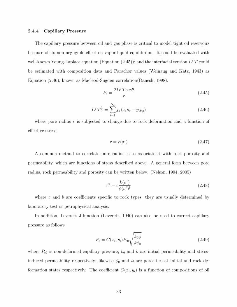
2.4.4 Capillary Pressure
The capillary pressure between oil and gas phase is critical to model tight oil reservoirs
because of its non-negligible effect on vapor-liquid equilibrium. It could be evaluated with
well-known Young-Laplace equation (Equation (2.45)); and the interfacial tension IFT could
be estimated with composition data and Parachor values (Weinaug and Katz, 1943) as
Equation (2.46), known as Macleod-Sugden correlation(Danesh, 1998).
Pc =2IFTcosθ
r(2.45)
IFT14 =
Nc∑i=1
χi (xiρo − yiρg) (2.46)
where pore radius r is subjected to change due to rock deformation and a function of
effective stress:
r = r(σ′) (2.47)
A common method to correlate pore radius is to associate it with rock porosity and
permeability, which are functions of stress described above. A general form between pore
radius, rock permeability and porosity can be written below: (Nelson, 1994, 2005)
r2 = ck(σ
′)
φ(σ′)b(2.48)
where c and b are coefficients specific to rock types; they are usually determined by
laboratory test or petrophysical analysis.
In addition, Leverett J-function (Leverett, 1940) can also be used to correct capillary
pressure as follows.
Pc = C(xi, yi)Pc0
√k0φ
kφ0
(2.49)
where Pc0 is non-deformed capillary pressure; k0 and k are initial permeability and stress-
induced permeability respectively; likewise φ0 and φ are porosities at initial and rock de-
formation states respectively. The coefficient C(xi, yi) is a function of compositions of oil
33

and gas phases, which supplement the composition differences between the reference fluid
for measuring Pc0 and current fluid.
2.4.5 Relative Permeability
Although there are experimental studies (Lai and Miskimins, 2010) and observations on
the change of relative permeability due to geomechanical effect as introduced in Chapter 1,
there are rarely developed model for the relationship between effective stress and relative
permeability. Lei et al. (2015) derived a fractal model; it relates relative permeability with
not only phase saturation, but also pore radius and fractal dimensions.
krβ = krβ (Sβ, r,D) (2.50)
where r and D are pore radius and fractal dimensions, which are functions of effective stress.
2.5 Summary and Discussions
This chapter introduces the mathematical model for a general compositional model and
a coupled geomechanical model. The compositional model is essentially a mass conservation
equation, which associates the mass flux and sink/source with mass accumulation. The way
to evaluation of each term of mass balance equation is also presented, including the flow
characteristics of tight reservoirs, such as gas molecular diffusion and Klinkenberg effect.
The derived geomechanical model couples reservoir pore pressure and mean stress for the
isothermal tight oil reservoir. In addition, the constitutive relations for the compositional
model are discussed. And this chapter concludes with the geomechanical effect on fluid flow
and rock properties.
Besides the mathematical description of compositional model, a robust computation
method for vapor-liquid equilibrium is required to calculate phase composition in order to
evaluate each term of the governing mass balance equation (Equation (2.1)); and the next
chapter will address this topic.
34

CHAPTER 3
VAPOR-LIQUID EQUILIBRIUM CALCULATION
Vapor-liquid equilibrium (VLE) calculation is required in compositional model in order
to obtain the phase composition and thermodynamic properties. This chapter discusses the
VLE calculation method involving the effect of capillary pressure. In addition, the Eagle
Ford tight oil is taken as the example to illustrate the VLE calculation procedure and the
non-negligible effect of capillary pressure on it.
3.1 Phase Equilibrium Calculations
Because of the assumption of no mass transfer between water and hydrocarbon phases, a
two-phase (oil and gas ) equilibrium calculation is required to obtain the phase composition
and finally to evaluate the general compositional model (mass balance equation). The theory
and computation procedures for VLE calculation are discussed below.
3.1.1 Theory of Phase Equilibrium Calculations
In a multi-component system under vapor-liquid equilibrium, the chemical potential µ of
each component i throughout all co-existing phases should be equal.
µoi = µgi i = 1, ..., nc (3.1)
This general requirement becomes a practical engineering tool if the chemical potential
can be related to measurable or calculable quantities, such as fugacity f (Danesh, 1998) as
follows.
f oi = f gi i = 1, ..., nc (3.2)
The practical way to calculate fugacity of each component is to evaluate the dimensionless
fugacity coefficient, Φ, which is defined as the ratio of fugacity to partial pressure of the
corresponding phase for component i by Equation (3.3).
35

Φoi =
f oixiP o
Φgi =
f giyiP g
i = 1, ..., nc (3.3)
The fugacity coefficient then can be calculated because it can be related rigorously to
measurable properties, such as pressure, temperature and volume, with thermodynamic re-
lations as Equation (3.4) (Danesh, 1998).
lnΦi =1
RT
∫ ∞V
[( ∂P∂Ni
)T,V,Nj 6=i
−RT/V]dV − lnz (3.4)
where R is gas constant, Ni is the number of moles of component i; V is the total volume,
and z is the mixture compressibility factor. Equation (3.4) can be determined with the aid
of an Equation of State (EOS), relating pressure, temperature, volume and compositions.
In this dissertation, Peng-Robinson (Peng and Robinson, 1976) Equation of State (PR
EOS) as below is used to evaluate lnΦi.
P =RT
V − b− a
V (V + b) + b(V − b)(3.5)
With the aid of Equation (3.5) and plugging it to Equation (3.4), lnΦoi and lnΦg
i can be
calculated as Equation (3.6) and (3.7).
lnΦoi =
bib
(z− 1)− ln(z− bP o
RT
)+
a
2√
2bRT
(2nc∑j=1
xjaij
a− bib
)ln
(z + (1−
√2) bP
o
RT
z + (1 +√
2) bPo
RT
)(3.6)
lnΦgi =
bib
(z− 1)− ln(z− bP g
RT
)+
a
2√
2bRT
(2nc∑j=1
yjaij
a− bib
)ln
(z + (1−
√2) bP
g
RT
z + (1 +√
2) bPg
RT
)(3.7)
where a and b are parameters defined by PR EOS; they are functions of components’ thermo-
dynamic properties, such as critical pressure and temperature, composition, acentric factor,
binary interaction coefficient, etc. Therefore fugacity coefficients are calculable with compo-
nent’s thermodynamic properties and corresponding phase pressure and temperature.
In addition to above method to calculate fugacity for the conditions of VLE, the method
to calculate composition of each phase at the condition of VLE is also required. A general
36

method is to solve Rachford-Rice (R-R) equation (Equation (3.8)) (Rachford Jr and Rice,
1952) with the input of equilibrium ratio Ki of component i, defined as Ki = yi/xi.
nc∑i=1
zi(Ki − 1)
no +Ki(1− no)= 0 (3.8)
Equation (3.8) takes overall molar fraction of oil and gas phases, zi, and equilibrium
ratio, Ki, of component i as input to calculate the molar fractions of oil and gas phase and
composition of each phase.
In the non-ideal system at equilibrium, Ki is usually related to fugacity coefficient by
combining of Equation (3.2) and (3.3) as follows.
(f oi = ΦoixiP
o) = (f gi = Φgi yiP
g)⇒ Ki =yixi
=P oΦo
i
P gΦgi
=P oΦo
i
(P o + Pcgo)Φgi
(3.9)
In conventional reservoirs, Equation (3.9) is simplified to Ki = Φoi/Φ
gi by assuming P o ≈
P g. However, this assumption is not valid for tight oil reservoirs due to large capillary
pressure Pcgo. Fugacity coefficient, Φ, in Equation (3.9) can be obtained with PR EOS as
Equation (3.6) and (3.7).
The overall VLE calculation requires iterative computation, because Equation (3.6) and
(3.7) can only be solved after solving Equation (3.8) for results of phase composition, which
in turn needs the Ki as input. Therefore an initial guess of Ki is required as the starting
point. Wilson’s correlation (Wilson, 1969) below is usually used to generate the initial guess
of Ki.
Ki = (Pci/P ) exp[5.37(1 + ωi)(1− Tci/T )
](3.10)
where ωi is the acentric factor of component i.
In addition, the capillary pressure between oil and gas phase Pcgo is also a function
of phase composition, the iterative computation also requires the calculation of capillary
pressure.
37

3.1.2 Flow Chart of Phase Equilibrium Calculations
Based on above discussions, the process for two-phase equilibrium calculation is summa-
rized in Figure 3.1. With initial values such as pressure, temperature and the thermodynamic
properties of each components, the initial guess for K values are obtained with Wilson’s equa-
tion (Equation (3.10)). With those K values as input, Equation (3.8) generate the results of
phase composition. With the phase composition, the phase compressibility factor Z is calcu-
lated with PR-EOS. Then the fugacity coefficient and fugacity are calculated with Equation
(3.6) and (3.7) before check the convergence criteria as follows.
nc∑i=1
(1− f oi /fgi )2 ≤ ε (3.11)
where ε is a very small number as the convergence criteria. The convergence criteria are
actually the condition where the oil and gas phases are at equilibrium described in Equation
(3.2).
If the convergence criteria is not met, K values and Pcgo are updated with the recent
calculated phase composition; if the convergence criteria is met, it means VLE is reached
and iteration stops.
3.2 Saturation Pressure Calculation
The initial pore pressure for tight oil reservoir is usually far above saturation pressure at
which there is no gas phase at reservoir condition. The VLE calculation procedure presented
above is able to check whether reservoir pressure is below saturation pressure or not through
calculating ΣziKi (Danesh, 1998). However, the VLE calculation requires large computation
efforts. This section presents a simpler method to calculate saturation pressure including
the effect of capillary pressure with PR-EOS.
Saturation pressure, or bubble-point pressure, is the pressure at which the first gas bubble
forms in oil phase. It poses two conditions at saturation pressure: oil composition is same
as the overall composition; and phases are at equilibrium. From the phase equilibrium
38

Figure 3.1: Two phase equilibrium calculation including the effect of capillary pressure.
39

condition, there are following relations.
nc∑i=1
yi =nc∑i=1
f giΦgiP
g=
nc∑i=1
f oiΦgiP
g= 1 (3.12)
From above equation, there are also following relations:
nc∑i=1
f oiΦgi
=nc∑i=1
ΦoixiP
o
Φgi
= P g = P o + Pcgo(xi, yi) (3.13)
where Pcgo is the capillary pressure between oil and gas phases, which is also a function of
phase composition xi, yi. Finally we obtain the following iterative relation for saturation
pressure:
P oiter+1 = P o
iter
nc∑i=1
Φoixi
Φgi
− Pcgo(xi, yi) = P oiter
nc∑i=1
Φoi zi
Φgi
− Pcgo(xi, yi) (3.14)
where iter is the iterative step to solve the saturation pressure; Φgi and Φg
i can be evaluated
with the aid of PR-EOS.
From the above iterative relation, Figure 3.2 summarizes the flow chart for the saturation
pressure calculation. An initial guess for saturation pressure is given, and the initial K values
can be calculated. Accordingly the phase composition can be easily obtained because xi is
same as zi; the phase composition is inputted to calculate fugacity and fugacity coefficients,
which are used to update K value, capillary pressure and saturation pressure until the system
reach equilibrium conditions.
Compared with VLE calculation procedure in Figure 3.1, there is no need to solve R−R
equation (Equation (3.8))) for phase composition, and the convergence speed is faster. There-
fore the calculation procedure of saturation pressure is used to check if reservoir pressure
decreases below saturation pressure; and the VLE calculation is only performed in the case
of reservoir pressure below saturation pressure.
3.3 Calculation Examples
A sample of Eagle Ford light oil is taken as the example to demonstrate above calculation
methods of VLE and saturation pressure. This example also illustrates the effect of capillary
40
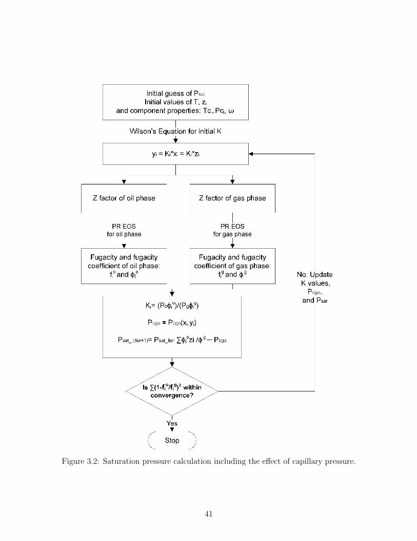
Figure 3.2: Saturation pressure calculation including the effect of capillary pressure.
41

pressure on saturation pressure and VLE. Table 3.1 and Table 3.2 lists the composition data
and thermodynamic properties of component of the sample oil of Eagle Ford tight reservoir
(Orangi et al., 2011).
Table 3.1: Eagle Ford oil composition and component properties
Component Molar Pc Tc vc Acentric MolarFraction (psi) ( ◦R) (ft3/lbmole) Factor Weight
C1 0.31231 673.1 343.3 1.5658 0.013 16.04N2 0.00073 492.3 227.2 1.4256 0.04 28.01C2 0.04314 708.4 549.8 2.3556 0.0986 30.07C3 0.04148 617.4 665.8 3.2294 0.1524 44.1
CO2 0.01282 1071.3 547.6 1.5126 0.225 44.01IC4 0.0135 529.1 734.6 4.2127 0.1848 58.12NC4 0.03382 550.7 765.4 4.1072 0.201 58.12IC5 0.01805 483.5 828.7 4.9015 0.2223 72.15NC5 0.02141 489.5 845.6 5.0232 0.2539 72.15NC6 0.04623 439.7 914.2 5.9782 0.3007 86.18C7+ 0.16297 402.8 1065.5 7.4093 0.3739 114.4C11+ 0.12004 307.7 1223.6 10.682 0.526 166.6C15+ 0.10044 241.4 1368.4 14.739 0.6979 230.1C20+ 0.07306 151.1 1614.2 26.745 1.0456 409.2
There are two methods for capillary pressure correlation discussed in Chapter 2, Young-
Laplace equation and J-function. In this example, Young-Laplace method is used and interfa-
cial tension is calculated with Macleod-Sugden correlation. Figure 3.3 presents the calculated
saturation pressure for the oil sample in three scenarios: without effect of capillary pressure,
20 nm pore radius and 10 nm pore radius. It shows that the saturation pressure is suppressed
due to capillary pressure, especially in the lower and middle temperature range. In the high
temperature range, the difference of saturation pressure caused by capillary pressure is small
because it is close to critical point, where there is no phase difference and interfacial tension
becomes zero.
The effect of capillary pressure on saturation pressure also results in more light compo-
nents dissolving in oil phase at the pressure below bubble-point because those light compo-
42

Table 3.2: Eagle Ford oil binary interaction parameters
C1 N2 C2 C3 CO2 IC4 NC4 IC5 NC5 NC6 C7+ C11+ C15+ C20+
C1 0 0.036 0 0 0.1 0 0 0 0 0 0.025 0.049 0.068 0.094N2 0.036 0 0.05 0.08 -0.02 0.095 0.09 0.095 0.1 0.1 0.151 0.197 0.235 0.288C2 0 0.05 0 0 0.13 0 0 0 0 0 0.02 0.039 0.054 0.075C3 0 0.08 0 0 0.135 0 0 0 0 0 0.015 0.029 0.041 0.056CO2 0.1 -0.02 0.13 0.135 0 0.13 0.13 0.125 0.125 0.125 0.11 0.097 0.085 0.07IC4 0 0.095 0 0 0.13 0 0 0 0 0 0.01 0.019 0.027 0.038NC4 0 0.09 0 0 0.13 0 0 0 0 0 0.01 0.019 0.027 0.038IC5 0 0.095 0 0 0.125 0 0 0 0 0 0.005 0.01 0.014 0.019NC5 0 0.1 0 0 0.125 0 0 0 0 0 0.005 0.01 0.014 0.019NC6 0 0.1 0 0 0.125 0 0 0 0 0 0 0 0 0C7+ 0.025 0.151 0.02 0.015 0.11 0.01 0.01 0.005 0.005 0 0 0 0 0C11+ 0.049 0.197 0.039 0.029 0.097 0.019 0.019 0.01 0.01 0 0 0 0 0C15+ 0.068 0.235 0.054 0.041 0.085 0.027 0.027 0.014 0.014 0 0 0 0 0C20+ 0.094 0.288 0.075 0.056 0.07 0.038 0.038 0.019 0.019 0 0 0 0 0
Figure 3.3: Saturation pressure (Bubble-point) of Eagle Ford oil.
43

nents evolves into gas phase at a lower pressure. Figure 3.4 shows the molar fraction of light
components, C1 and C2, in oil phases under different pore radius at pressure of 1200 psi
and 1500 psi, both below saturation pressure.
Figure 3.4: Molar fraction of C1 + C2 in oil phase.
The effect on composition of oil phase further leads to the influence on fluid properties,
such as oil density and viscosity. The light components in oil phase lead to lighter oil
density and smaller viscosity shown in Figure 3.5, where the viscosity is calculated with with
Lohrenz-Bray-Clark(LBC) correlation (Lohrenz et al., 1964). The oil density and viscosity
at 1200 psi and 1500 psi decrease as pore radius decrease due to an increase of capillary
pressure.
3.4 Summary and Discussions
This chapter presents the theory, methods and calculation procedures for VLE and sat-
uration pressure, involving the capillary pressure effect. And a light oil sample from Eagle
Ford reservoir is taken as the example to illustrate computation process and the effect of cap-
44

(a) Oil density (b) Oil viscosity
Figure 3.5: Oil density and viscosity under capillarity effect.
illary pressure. It is observed that the capillary pressure suppresses the saturation pressure,
and accordingly influence the phase composition and fluid properties.
However, the reservoir production is a dynamic process, where the overall composition
z, reservoir pressure, and pore radius, etc. are changing during fluid depletion. Thus the
compositional model with above VLE calculation method is required to simulate and capture
the fluid flow behaviors of tight oil reservoir. The next chapter will address the numerical
solution in order to solve the compositional model with numerical methods.
45
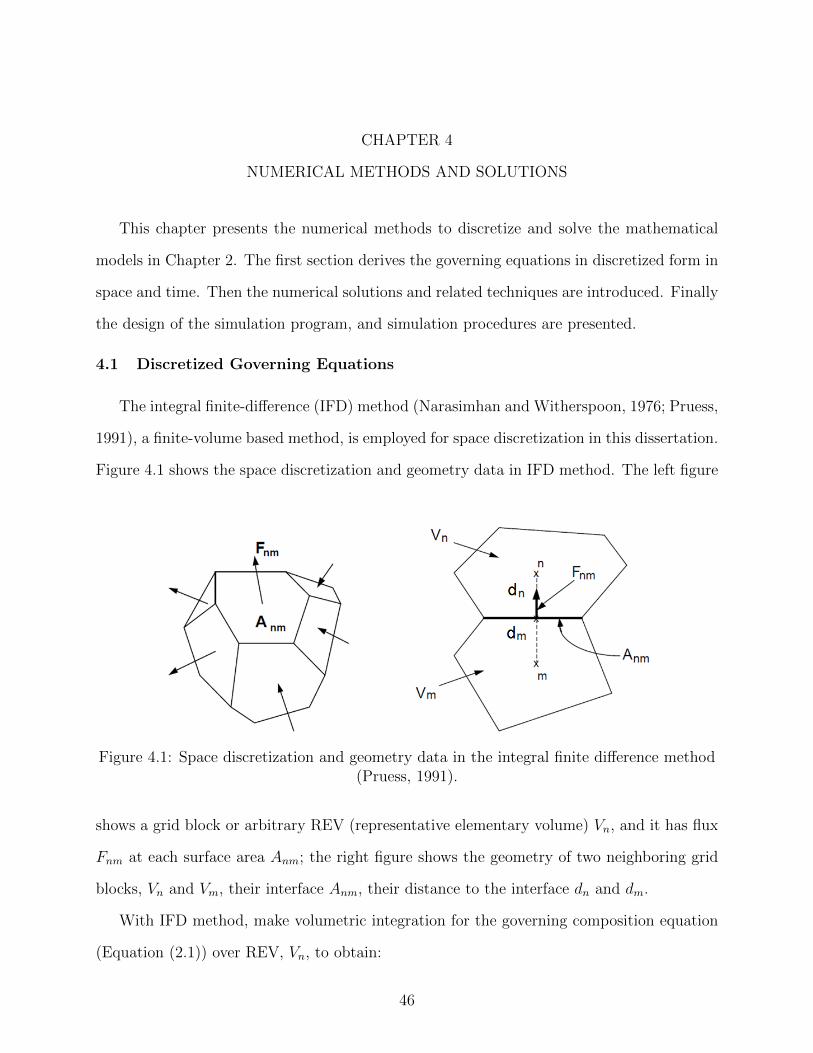
CHAPTER 4
NUMERICAL METHODS AND SOLUTIONS
This chapter presents the numerical methods to discretize and solve the mathematical
models in Chapter 2. The first section derives the governing equations in discretized form in
space and time. Then the numerical solutions and related techniques are introduced. Finally
the design of the simulation program, and simulation procedures are presented.
4.1 Discretized Governing Equations
The integral finite-difference (IFD) method (Narasimhan and Witherspoon, 1976; Pruess,
1991), a finite-volume based method, is employed for space discretization in this dissertation.
Figure 4.1 shows the space discretization and geometry data in IFD method. The left figure
Figure 4.1: Space discretization and geometry data in the integral finite difference method(Pruess, 1991).
shows a grid block or arbitrary REV (representative elementary volume) Vn, and it has flux
Fnm at each surface area Anm; the right figure shows the geometry of two neighboring grid
blocks, Vn and Vm, their interface Anm, their distance to the interface dn and dm.
With IFD method, make volumetric integration for the governing composition equation
(Equation (2.1)) over REV, Vn, to obtain:
46

∫Vn
−∇ · (ρoxi~vo + ρgyi~vg)dV +
∫Vn
∇ · (Deff,i∇ (ρgyi)) dV +
∫Vn
qidV
=
∫Vn
∂φ(ρoSoxi + ρgSgyi)dV
∂t(4.1)
Apply divergence theorem for above equation to convert volume integral to surface integral
for flux term:
∫Γn
−(ρoxi~vo + ρgyi~vg) · ndΓ +
∫Γn
Deff,i∇(ρgyi) · ndΓ +
∫Vn
qidV =∫Vn
∂φ(ρoSoxi + ρgSgyi)dV
∂t(4.2)
where Γn is the surface areas of the grid block and n is the outward pointing unit vector
normal to the boundary. Equation (4.2) is readily to be discretized as below.
Volume integrals are replaced with volume average and surface integral is evaluated with
discrete sum over surface average segments.
∑m∈ηn
(ρoxi~vo nm + ρgyi~vg nm)Anm +∑m∈ηn
Deff,i∇ (ρgyi)nmAnm + Vnqi
=d[Vnφ(ρoSoxi + ρgSgyi)
]dt
(4.3)
where ~vo nm is the oil flow from grid block n to m, similarly for ~vg nm; ηn is all neighboring
grid blocks directly connecting grid blocks n and Anm is the interface area between them;
∇(ρgyi)nm is the concentration gradient between grid block n and m.
Apply Darcy’s law (Equation (2.7)) to above equation, and the time is discretized fully
implicitly to assure stability. The above equation is finally discretized in space and time as
below.
47

∑m∈ηn
[(ρoxiλo)
t+1nm+ 1
2
γt+1nm (Ψt+1
om −Ψt+1on ) + (ρgyiλg)
t+1nm+ 1
2
γt+1nm (Ψt+1
gm −Ψt+1gn )]
+∑m∈ηn
Deff,iAt+1nm
(ρgyi)t+1m − (ρgyi)
t+1n
dt+1n + dt+1
m
+ (V qi)t+1n =
[V φ(ρoSoxi + ρgSgyi)]t+1n − [V φ(ρoSoxi + ρgSgyi)]
tn
∆t(4.4)
where λ is the phase mobility defined as λβ = krβ/µβ for phase β; Ψ is the flow potential
including both pressure and gravity term Ψt+1βn = P t+1
βn −ρt+1βnm+ 1
2
gZn; subscript nm+ 12
denotes
a proper averaging at the interface between n and m; t+ 1 is the current time step and t is
the previous time step. γ is the transmissivity defined as
γt+1nm =
(Anmknm+ 1
2
dn + dm
)t+1
(4.5)
The water component has similar but simpler form of discretized equation as hydrocarbon
component:
∑m∈ηn
[(ρwλw)t+1
nm+ 12
γt+1nm (Ψt+1
wm −Ψt+1wn )]
+ (V qw)t+1n =
(V φρwSw)t+1n − (V φρwSw)tn
∆t(4.6)
Equation (4.4) and (4.6) are the final equations discretized fully implicitly for hydrocar-
bon components and water. Different from conventional fully implicit method, the geometry
of grid blocks, such as the volume V , interface area Anm, connection distance dn, dm are
subjected to change due to geomechanical effect. Thus those geometry variable and flow
transmissivity γnm are evaluated at each time step t+ 1.
The geomechanical governing equation can also be discretized with IFD method with
similar procedure (Winterfeld and Wu, 2013; Xiong et al., 2013). Take volume integral on
Equation (2.21) and apply divergence theorem on it to get the following surface integral
form: ∫Γn
[3(1− ν)
1 + ν∇σmean + F b −
2(1− 2ν)
1 + ν∇αP
]· ndΓn = 0 (4.7)
48

The surface integral can be evaluated with discrete sum over surface average segments
at current time step.
∑m∈ηn
[3(1− ν)
1 + ν
σt+1n − σt+1
m
dnm+ (F b · n)nm −
2α(1− 2ν)
1 + ν
P t+1n − P t+1
m
dnm
]At+1nm = 0 (4.8)
Equation (4.8) is the discretized stress equation with mean stress σ as geomechanical variable
and coupled with reservoir pore pressure P as the fluid flow variable.
4.2 Boundary Conditions and Well Treatments
A similar method to MSFLOW, big-volume method, is taken to treat the first-type
boundary conditions, denoting constant phase pressure and constant saturation conditions.
The volume of boundary grid block is set to infinity, such as 1050 m3, and the conditions
of constant pressure and saturations are automatically met during the simulation. And the
flux-type boundary conditions are simply treated as sink/source terms in Equation (4.4).
For a grid block n connected to a well with constant production pressure Pwell, its
sink/source term for hydrocarbon and water components can be evaluated as following.
(qi)t+1n = (ρoxiλo)
t+1n WI
(P t+1on − Pwell
)+ (ρgyiλg)
t+1n WI
(P t+1gn − Pwell
)(4.9)
(qw)t+1n = (ρwλw)t+1
n WI(P t+1wn − Pwell
)(4.10)
where WI is the well index, mainly relating with the permeability and geometry of the grid
block n, and well skin factor.
The constant boundary condition is used to treat geomechanical model, where boundary
grid blocks have constant mean stress. Usually boundary grid blocks are the borders of a
reservoir. For a geomechanical boundary grid block n, Equation (4.8) is simplified to
3(1− ν)
1 + ν
σt+1n − σ0
n
2dn= 0 (4.11)
to denote the constant stress of grid block n.
49

4.3 Numerical Solution Technique
This section discusses how to solve above discretized equations, including residual form
of discretized equations, freedom of degree analysis and primary variables selections.
4.3.1 Residual Form
The discretized governing equations for hydrocarbon components i, water w and mean
stress σmean can be written in residual forms. Equation (4.4), (4.6) and (4.8) are rewritten
as below.
Rt+1i,n =
[V φ(ρoSoxi + ρgSgyi)]t+1n − [V φ(ρoSoxi + ρgSgyi)]
tn
∆t
−∑m∈ηn
[(ρoxiλo)
t+1nm+ 1
2
γt+1nm (Ψt+1
om −Ψt+1on ) + (ρgyiλg)
t+1nm+ 1
2
γt+1nm (Ψt+1
gm −Ψt+1gn )]
−∑m∈ηn
Deff,iAt+1nm
(ρgyi)t+1m − (ρgyi)
t+1n
dt+1n + dt+1
m
− (V qi)t+1n = 0 (4.12)
Rt+1w,n =
(V φρwSw)t+1n − (V φρwSw)tn
∆t−∑m∈ηn
[(ρwλw)t+1
nm+ 12
γt+1nm (Ψt+1
wm −Ψt+1wn )]−(V qw)t+1
n = 0
(4.13)
Rt+1σ,n =
∑m∈ηn
[3(1− ν)
1 + ν
σt+1n − σt+1
m
dnm+ (F b · n)nm −
2α(1− 2ν)
1 + ν
P t+1n − P t+1
m
dnm
]At+1nm = 0
(4.14)
Equation (4.12), (4.13) and (4.14) are coupled non-linear equation system for one grid
block Vn, and there are total nc + 2 independent equations (nc for hydrocarbon component,
1 for water and 1 for stress) for each grid block.
4.3.2 Degrees of Freedom and Primary Variables
The degrees of freedom of a system means the number of variables required to fix the
intensive state of the system. According to Gibbs phase rule, for a compositional system with
50

total number nm of components and np of phases, the thermodynamic degrees of freedom
are nm + 2 − np. On the other hand, there are also np − 1 saturation degrees of freedom
due to phase saturation constrained by ΣSβ = 1(β = 1, ..., np). Thus the final degrees
of freedom (Cao, 2002; Pruess, 1991) for an isothermal compositional system is the sum
of thermodynamic degrees of freedom plus saturation degrees of freedom, and minus the
temperature as follows.
f = (nm + 2− np) + (np − 1)− 1 = nm (4.15)
where nm is the number of total mass component and np is the number of phases in the
system. In this dissertation nm = nc + 1, the sum of hydrocarbon and water components.
Mean stress σmean is another degree of freedom in the coupled geomechanics model. Thus
there are nc + 2 degrees of freedom for the compositional model coupled with geomechanics
in this dissertation, which means there are nc + 2 variables required to solve in the system.
The minimum number of independent variables needed to be solved is the same number
of the degrees of freedom nc+2 in the system. There is a variety of ways to select the primary
variables for a compositional model (Cao, 2002); some of them may need to switch primary
variables during simulation dependent on the current number of phases in the system (Coats,
1980); some of them treat phase equilibrium variables as primary variables (Pan, 2009;
Santos, 2013; Wang et al., 1997). Collins et al. (1992) pointed out that phase equilibrium
calculation is by itself a difficult task and it added a high level of complexity to final solutions
for solving flow and equilibrium simultaneously.
The selection of primary variables in this dissertation minimizes the complexity intro-
duced by phase appearance/disappearance and VLE calculation. Thus the primary variables
chosen in this dissertation are water saturation, reservoir pressure, overall molar fraction of
each component, and mean stress, described below.
xn = (Sw, Po, z1, ..., znc−1, σmean) (4.16)
where xn is the primary variable vector for grid block Vn.
51

The above primary variables are independent from the existing number of phases of the
system, and there is no need to switch primary variable during the simulation. It is robust
to handle the phase appearance and disappearance. These variables are also independent
from VLE calculations; thus it provides the flexibility to adapt different methods of VLE
calculations in the numerical implementation.
4.3.3 Determination of Secondary Variables
Other fluid and rock related properties interested in the model are considered as secondary
variables, which can be determined with the constitutive relations discussed in Chapter 2
once the primary variables are solved.
The phase composition xi, yi, no and ng can be determined with T , P , and overall
composition zi as the input for VLE calculation. With phase composition solved, the phase
viscosity can be calculated with correlations. In addition, the phase molar density ρo and ρg
can be solved with PR EOS. After solution of phase molar fraction no, ng and phase molar
density ρo, ρg, the volume fractions of oil and gas phase is determined, which are combined
with the primary variable Sw to obtain oil and gas saturations So and Sg. With phase
saturation in the place, the relative permeability and capillary pressure can be determined.
The secondary variables related to rock deformation, such as volumetric strain, rock porosity
and permeability etc., can also be calculated with primary variables of mean stress and
reservoir pressure. Figure 4.2 shows the brief calculation process for secondary variables
determination.
4.3.4 Solution Method
With above nc + 2 primary variables of one grid block, the same number of independent
equations are required to solve them. The discretized equations in residual form, Equation
(4.12), (4.13) and (4.14) are the independent equations in the system to solve the corre-
sponding primary variables. Table 4.1 summarizes the primary variables and corresponding
non-linear residual equations.
52

Figure 4.2: Process for secondary variable calculation.
Table 4.1: Primary variables and associated equations
Equations Primary variables Physical Meaning
Equation (4.13): Rt+1w,n
(Water mass balance)Sw Water saturation
Equation (4.12): Rt+1i,n
(Hydrocarbon compo-nents mass balance)
Po, z1, ..., znc−1 Oil phase pressure &Overall molar frac-tion
Equation (4.14): Rt+1σ,n
(Mean stress equation)σmean Mean stress
53

The above equations are solved with Newton/Raphson method. For the grid block n and
one of its non-linear equation at time step t+ 1, Rt+1κ,n , where κ = 1, ..., nc + 2 is the index of
the non-linear equation of grid block n, the Newton/Raphson scheme give rise to
Rt+1κ,n
(xt+1p+1
)= Rt+1
κ,n
(xt+1p
)+∑k
∂Rt+1κ,n
(xt+1p
)∂xk
(xk,p+1 − xk,p) = 0 (4.17)
where k is the index of primary variable of grid block n, and k = 1, 2, ..., nc + 2; p is the
iteration level of current time step t+ 1. Equation (4.17) can be written as
∑k
∂Rt+1κ,n
(xt+1p
)∂xk
δxk,p+1 = −Rt+1κ,n
(xt+1p
)(4.18)
where δxk,p+1 = xk,p+1 − xk,p. Assume that there is total nb grid blocks in the simulation
domain, there are total nb× (nc + 2) equations like Equation (4.18). Those equations stands
for a linear equation system with the increments δxk,p+1 as the unknown to be solved; and the
coefficients, ∂Rt+1κ,n
(xt+1p
)/∂xk, forms a Jacobian matrix of size nb× (nc+2) by nb× (nc+2).
The derivatives, ∂Rt+1κ,n
(xt+1p
)/∂xk, can be obtained with numerical differentiation method.
A small incremental value ∆xk is added to the corresponding primary variable, and the
secondary variables are re-evaluated with the incremental primary variables; finally a new
residual value, Rt+1κ,n , is obtained to calculate the derivatives numerically as follows.
∂Rt+1κ,n
(xt+1p
)∂xk
=Rt+1κ,n
(xt+1p + ∆xk
)−Rt+1
κ,n
(xt+1p
)∆xk
(4.19)
In general, the derivatives with sufficient accuracy can be obtained with ∆xk set as 10−6 to
10−8 of current value of xk.
4.4 Program Implementation
Based on above discussion about numerical discretization and solution methods, this
section describes the implementation of the numerical program. The program is developed
based on an existing black-oil simulation program MSFLOW (Wu, 1998); and the imple-
mented program in this dissertation is named to MSFLOW COM with the capability of
compositional and geomechanical modeling.
54

Figure 4.3 shows the core modules and their relationship for the implemented simulation
program. Below is the brief description for each module.
• Liner solver: it solves the linearized equation system (Equation (4.18)).
• Jacobian matrix building & Newton iteration control: it assemblies the Jacobian matrix
with numerical differentiation and controls the Newton/Raphson iterations. And the
numerical differentiation requires the values of secondary variables for current primary
variables.
• VLE calculation & Secondary variable computation: this module is the implementation
of Figure 4.2; it calculates the VLE and secondary variables.
• Data input & Initialization: it read the input data and initialize them ready for the
simulation.
• Simulation control: it mainly controls the time steps.
• Output: it outputs the simulation results.
Figure 4.3 also shows one Newton/Raphson iteration involving building Jacobian matrix,
solving the linear system and calculating VLE and secondary variables in the left box the
figure.
With above core modules, Figure 4.4 shows the whole simulation process. After the
input data is initialized, the time loop starts. For each time step, it usually requires a
variety number of Newton iterations until the convergence criteria are reached. And the
convergence criteria are only reached if all the primary variables for all grid blocks in the
simulation domain are converged. If the convergence criteria are not met, the iteration
continues; and the time loop moves to next time step if the simulation results of current
time step are converged.
55

Figure 4.3: Core modules and their relationships of MSFLOW COM.
56

Figure 4.4: Simulation process of MSFLOW COM.
57
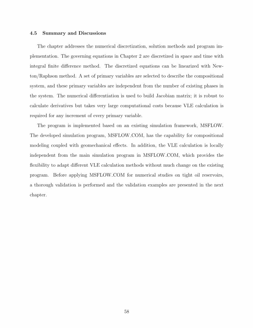
4.5 Summary and Discussions
The chapter addresses the numerical discretization, solution methods and program im-
plementation. The governing equations in Chapter 2 are discretized in space and time with
integral finite difference method. The discretized equations can be linearized with New-
ton/Raphson method. A set of primary variables are selected to describe the compositional
system, and these primary variables are independent from the number of existing phases in
the system. The numerical differentiation is used to build Jacobian matrix; it is robust to
calculate derivatives but takes very large computational costs because VLE calculation is
required for any increment of every primary variable.
The program is implemented based on an existing simulation framework, MSFLOW.
The developed simulation program, MSFLOW COM, has the capability for compositional
modeling coupled with geomechanical effects. In addition, the VLE calculation is locally
independent from the main simulation program in MSFLOW COM, which provides the
flexibility to adapt different VLE calculation methods without much change on the existing
program. Before applying MSFLOW COM for numerical studies on tight oil reservoirs,
a thorough validation is performed and the validation examples are presented in the next
chapter.
58
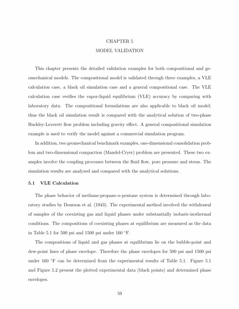
CHAPTER 5
MODEL VALIDATION
This chapter presents the detailed validation examples for both compositional and ge-
omechanical models. The compositional model is validated through three examples, a VLE
calculation case, a black oil simulation case and a general compositional case. The VLE
calculation case verifies the vapor-liquid equilibrium (VLE) accuracy by comparing with
laboratory data. The compositional formulations are also applicable to black oil model;
thus the black oil simulation result is compared with the analytical solution of two-phase
Buckley-Leverett flow problem including gravity effect. A general compositional simulation
example is used to verify the model against a commercial simulation program.
In addition, two geomechanical benchmark examples, one-dimensional consolidation prob-
lem and two-dimensional compaction (Mandel-Cryer) problem are presented. These two ex-
amples involve the coupling processes between the fluid flow, pore pressure and stress. The
simulation results are analyzed and compared with the analytical solutions.
5.1 VLE Calculation
The phase behavior of methane-propane-n-pentane system is determined through labo-
ratory studies by Dourson et al. (1943). The experimental method involved the withdrawal
of samples of the coexisting gas and liquid phases under substantially isobaric-isothermal
conditions. The compositions of coexisting phases at equilibrium are measured as the data
in Table 5.1 for 500 psi and 1500 psi under 160 ◦F.
The compositions of liquid and gas phases at equilibrium lie on the bubble-point and
dew-point lines of phase envelope. Therefore the phase envelopes for 500 psi and 1500 psi
under 160 ◦F can be determined from the experimental results of Table 5.1. Figure 5.1
and Figure 5.2 present the plotted experimental data (black points) and determined phase
envelopes.
59

Table 5.1: Experimentally Determined Compositions (Dourson et al., 1943)
Pressure (psi) Gas Phase Liquid Phase
500
Methane Propane n-Pentane Methane Propane n-Pentane
0.768 0.106 0.126 0.119 0.141 0.7400.736 0.152 0.112 0.121 0.175 0.7040.661 0.238 0.101 0.116 0.259 0.6250.563 0.350 0.087 0.107 0.421 0.4720.524 0.406 0.070 0.103 0.474 0.4230.485 0.439 0.076 0.098 0.522 0.3800.352 0.595 0.053 0.075 0.693 0.232
15000.798 0.105 0.097 0.401 0.181 0.4180.679 0.223 0.098 0.414 0.321 0.2650.634 0.272 0.094 0.434 0.357 0.209
In order to validate the VLE calculation of simulation program, a series of compositions
of coexisting phases are calculated with the properties of each component as Table 5.2,
where Pc and Tc are critical pressure and temperature respectively. Similarly the calculated
compositions of liquid and gas phases at equilibrium should lie on the bubble-point and
dew-point lines of phase envelope.
The calculated results are also plotted in Figure 5.1 and Figure 5.2 as red points to
compare with the experimentally determined phase envelope. It is shown that the calculated
results match well with the phase envelopes under both 500 psi and 1500 psi at 160 ◦F.
Table 5.2: Component properties used for validation of VLE calculation
Pc Tc Molar Weight Accentric Interaction Coefficients(MPa) (K) (g/gmol) Factor Methane Propane n-Pentane
Methane 4.599 190.56 16.043 0.0115 0.0 0.0140 0.0236Propane 4.248 369.83 44.096 0.1523 0.0140 0.0 0.0120
n-Pentane 3.370 469.70 72.150 0.2515 0.0236 0.0120 0.0
60
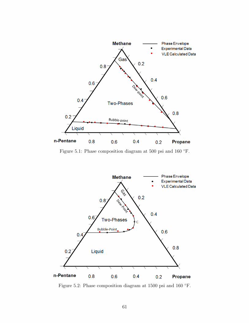
Figure 5.1: Phase composition diagram at 500 psi and 160 ◦F.
Figure 5.2: Phase composition diagram at 1500 psi and 160 ◦F.
61

5.2 Black Oil Model
Compositional formulations presented in Chapter 2 can also be used to model black
oil system where water, gas and oil at standard condition are considered as three pseudo-
components. Section 5.1 validates the accuracy of VLE calculation and this section further
validates the computation accuracy of numerical simulation framework.
5.2.1 Black Oil Model Simulation with Compositional Formulation
The general mass balance equation, Equation (2.1), holds for black oil system where
water, gas and oil at standard conditions are treated as mass components. The method to
evaluate accumulation, flux and sink/source terms for compositional model is also applicable
to black oil model except that mass is evaluated in molars for compositional model and in
bulk mass for black oil model. Therefore the black oil model can be treated as a simpli-
fied compositional model where there is no VLE calculation required to compute secondary
properties, such as phase density, component mass fraction and viscosity etc. Instead those
secondary properties can be calculated with given PVT properties, such as formation volume
factors and gas solubility.
Based on above analysis, the residual form of general compositional formulation, Equation
(4.12) as below, still holds for black oil model.
Rt+1i,n =
[V φ(ρoSoxi + ρgSgyi)]t+1n − [V φ(ρoSoxi + ρgSgyi)]
tn
∆t−∑
m∈ηn
[(ρoxiλo)
t+1nm+ 1
2
γt+1nm (Ψt+1
om −Ψt+1on ) + (ρgyiλg)
t+1nm+ 1
2
γt+1nm (Ψt+1
gm −Ψt+1gn )]− (V qi)
t+1n = 0
where i = g and o are gas and oil components at stand conditions.
For a block oil system, the surface gas can exist in both gas and oil phases as free gas and
dissolved gas under reservoir conditions. The surface oil can only exist in oil phase. Thus
the secondary properties in above equation can be evaluated as following:
ρg =ρg
Bg(p)(5.1)
62

ρo =ρo + ρgRg,o(p)
Bo(p)(5.2)
xg =ρgRg,o(p)
ρo + ρgRg,o(p)(5.3)
xo =ρo
ρo + ρgRg,o(p)(5.4)
yg = 1 yo = 0 (5.5)
where ρβ is the density of phase β at standard conditions, which is usually given as in-
put for black oil model. Phase formation volume factor, Bg and Bo, and gas solubility R
are functions of pressure only, and usually given as table inputs. Thus the compositional
simulation framework can be applied for black oil simulation with above equations to cal-
culate secondary variables; accordingly the black oil model can be employed to validate the
compositional simulation framework.
5.2.2 Buckley-Leverett Two-phase Vertical Flow
The black oil model used in this dissertation to validate the compositional simulation
framework is the classical one-dimensional Buckley-Leverett flow problem including gravity
effect for which an analytical solution is available (Buckley and Leverett, 1941; Wu et al.,
1993). In this analytical solution, both fluids and porous medium are assumed to be incom-
pressible and capillary effects are neglected.
The simulation example reproduces the Buckley-Leverett problem with water injection
into a vertical porous medium column with 200 meter height and a unit cross-section area.
Initially the porous medium is saturated uniformly with 80% oil, 20% water and no gas.
Water is injected into the top boundary at a constant rate of 2.0× 10⁻⁶ m3/s. The rock and
fluid properties are summarized in Table 5.3.
The simulation domain is divided into 100 uniform grid blocks and the bottom boundary
is described a constant pressure of 1 bar as shown in Figure 5.3 (a). The Brooks-Corey
function (Honarpour et al., 1986) with the exponent equal to 1 is used to calculate relative
63

Table 5.3: Rock and fluid properties of Buckley-Leverett vertical flow problem
Parameter Value Unit
Permeability 1.0× 10⁻¹² m2
Porosity 0.3Cross-section area 1.0 m2
Residual water saturation 0.2Irreducible oil saturation 0.2Water viscosity 1.139× 10⁻³ Pa.sOil viscosity 4.0× 10⁻³ Pa.sWater density 1,000 kg/m3
Oil density 864 kg/m3
Water injection rate 2.0× 10⁻⁶ m3/sOil formation volume factor 1.0Water formation volume factor 1.0
(a) Buckley-Leverett vertical flowproblem description
(b) Simulation results and analytical solution
Figure 5.3: Buckley-Leverett vertical flow problem and result.
64

permeability of water and oil phases.
It is noted that this simulation case is a simplified black oil model, where oil and water
formation volume factors are constant as 1.0, and the three-phase formulation collapses into a
two-phase one. However, the general compositional formulation and corresponding equations
for black oil model, Equations (5.1) - (5.5), still hold.
The numerical simulation gives the water saturation profile along the column after 100
days of water injection, which is compared with the analytical solution shown in Figure 5.3
(b). The numerical and analytical results are in good agreement in spite of some smearing
at the sharp displacement front of the numerical solution.
5.3 A General Compositional Model
A general compositional simulation case is studied with a commercial simulator GEM of
Computer Modeling Group Ltd (CMG, 2012) and the developed program MSFLOW COM.
The studied reservoir is a 200-meter by 200-meter square with 6-meter thick and divided into
100 grid blocks in two dimensions as shown in Figure 5.4. There are total four hydrocarbon
components in the reservoir with initial pressure 2500 psi and constant temperature of 80
◦C. A production well is located at center of node 1 with constant flowing bottom hole
pressure of 500 psi. Table 5.4 and Table 5.5 list the reservoir properties and thermodynamic
properties of hydrocarbon components in the simulation.
The effects of capillary pressure on VLE calculation are not included in the example
because GEM neglects those effects. The same relative permeability curves are used in two
simulators, where water relative permeability is the function of water saturation only, and
gas relative permeability is sole function of gas saturation. The Stone method II (Aziz
and Settari, 1979) is used to determine oil relative permeability from the two-phase relative
permeability curves. A simple viscosity model is used in the simulations in which the oil and
gas viscosity are assumed to be a function of component compositions.
Total 1000 days simulation is performed; and simulation results, including reservoir pres-
sure and phase saturations, of well node, Node 1, and observed node, Node 100 in Figure 5.4,
65

(a) Reservoir geometry and production well (b) Simulation domain and mesh
Figure 5.4: Compositional simulation example description.
and accumulated productions are plotted and compared.
Table 5.4: Rock and fluid properties used for compositional simulations
Parameter Value Unit
Permeability 20.0 mdPorosity 0.1Residual water saturation 0.23Initial water saturation 0.30Irreducible oil saturation 0.36Critical gas saturation 0.02Constant bottom hole pressure 500 psiWater viscosity 1.139 cPWater density 62.43 lb/ft3
Rock compressibility 1.0× 10⁻⁶ psi−1
Figure 5.5 compares the reservoir pressure and gas saturation of node 1 and 100 simulated
by MSFLOW COM and GEM. The initial reservoir pressure is above bubble-point pressure
with initial gas saturation as zero. The pressure of well node decreases very fast immediately
after the production. And its gas saturation increases because its pressure quickly drops to
below the saturation pressure. The water and oil two-phase flow of Node 100 evolves to three
66

Table 5.5: Hydrocarbon component properties used for compositional simulations
Pc Tc Vc Molar Weight Accentric Initial Global(MPa) (K) (m3/kg-mol) (g/gmol) Factor Composition
Methane (CH4) 4.600 190.56 0.099 16.043 0.0115 0.3n-Butane (NC4) 3.799 425.20 0.255 58.124 0.2010 0.2n-Hexane (NC6) 2.969 507.40 0.370 86.178 0.3007 0.2
C11+ 2.122 679.78 0.667 166.600 0.5260 0.3
phases in about 70 days when its pressure drop to bubble-point pressure shown in Figure 5.5
(b). Figure 5.6 presents the comparisons of oil and water saturations of Node 1 and 100.
The saturations quickly decrease in well node due to large drawdown pressure.
Figure 5.5 and Figure 5.6 shows that the two simulators give almost same simulation
results for pressure decrease, the gas evolution and decrease profile of oil and water satura-
tions.
(a) Reservoir pressure (b) Gas saturation
Figure 5.5: Comparison of reservoir pressure and gas saturation of Node 1 and 100.
In addition to the simulation results of Node 1 and 100, the accumulated mass produc-
tion of each component is also compared to verify the mass conservations and computation
accuracy of well production. Figure 5.7 presents the accumulated production of each hy-
67
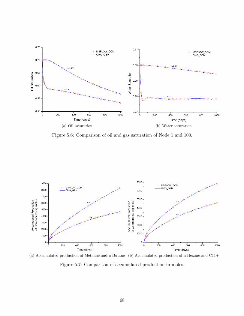
(a) Oil saturation (b) Water saturation
Figure 5.6: Comparison of oil and gas saturation of Node 1 and 100.
(a) Accumulated production of Methane and n-Butane (b) Accumulated production of n-Hexane and C11+
Figure 5.7: Comparison of accumulated production in moles.
68

(a) Accumulated production of oil at surface condition (b) Accumulated production of gas at surface condition
(c) Accumulated production of water at surfacecondition
Figure 5.8: Comparison of accumulated production at surface condition.
69

drocarbon component in moles. In order to verify the accuracy of VLE calculation under
surface condition of MSFLOW COM, I also compare the accumulated volumetric produc-
tion of water, oil and gas at surface condition (15.555 ◦C and 1 atm) as shown in Figure 5.8.
Both Figure 5.7 and Figure 5.8 shows the good agreements between MSFLOW COM and
CMG GEM for mass production and volumetric production at surface condition.
5.4 One-dimensional Consolidation
In this one-dimensional consolidation problem, a constant stress is applied to the top of
a porous permeable column fully saturated with water. The loaded stress instantaneously
induces the rock deformation and pore pressure increase of the column. Then fluid is allowed
to drain out of the column from top and the pore pressure increase dissipates. Accordingly
there are two steps to simulate above process. The first step is to simulate the pore pressure
increase due to the load on the top of the column, which is under undrained condition. The
second step is to set sink on the top of the column to simulate draining process, where the
dissipation of pore pressure increase happens. An analytical solution (Jaeger et al., 2007) is
available for the dissipation of pore pressure increase, which is used to verify the numerical
results.
Figure 5.9 illustrates both undrained condition and the drained process. Figure 5.9 (a)
is the initial state without external load and compaction. Figure 5.9 (b) is the equilibrated
state of pore pressure increase induced by instantaneous loaded stress without fluid drainage.
Figure 5.9 (c),(d) and (e) illustrate the drainage process, where a sink is set on the top of
column to allow the fluid flow. The increase of pore pressure quickly vanishes due to fluid
drainage and finally the pore pressures in the column return to the initial values.
Table 5.6 lists the input parameters used for the simulation, including rock mechanical
properties, fluid properties and initial and boundary conditions. The simulation domain is
a 100-meter long vertical column divided into 400 nodes. The simulation captures the dis-
sipation process of pore pressure increase and gives the pore pressure profile of the vertical
column during the drainage process. Figure 5.10 presents the comparison of pressure profile
70

Figure 5.9: One-dimensional consolidation processes under constant load.
Table 5.6: Rock and fluid properties of 1-D consolidation problem
Parameter Value Unit
Rock propertiesPermeability 1× 10⁻¹³ m2
Porosity 0.1Rock compressibility 7.4× 10⁻¹⁰ Pa−1
Young’s modulus 5× 10⁹ PaPoisson’s ratio 0.25Biot coefficient 1.0
Fluid propertiesWater density at standard condition 1000.0 kg/m3
Water viscosity 0.89× 10⁻³ Pa.sWater compressibility 4.5× 10⁻¹⁰ Pa−1
Initial and boundary conditionsInitial pore pressure 3.0× 10⁶ PaInitial stress 5.0× 10⁶ PaAdditional stress on the top 2.0× 10⁶ Pa
71

after 500, 6000 and 10000 seconds fluid drainage. It shows good agreement between simula-
tion results and analytical solutions for the dissipation process of pore pressure increase.
Figure 5.10: Pore pressure profile during drainage process under constant load.
5.5 Two-dimensional Compaction
The two-dimensional compaction problem is similar to one-dimensional consolidation
example. A constant compressive force is applied to the top of a fluid-filled porous medium
72

and it induces an instantaneous uniform pore pressure increase and rock compaction. The
lateral sides are free from either normal or shear stress. Afterwards, the material is allowed
to drain laterally. The pore pressure near the edges of two sides must decrease due to
drainage; therefore the material at the edges of two sides becomes less stiff and there is a
load transfer to the center, resulting in a further increase of pore pressure in the center of
the specimen. Thus the pore pressure in the center reaches a maximum and then declines.
This behavior of pore pressure evolution in the center is called Mandel-Cryer effect (Cryer,
1963) and Abousleiman et al. (1996) present an analytical solution for it.
(a) A constant stress on the top (b) Fluid lateral drainage
Figure 5.11: Problem description of two-dimensional compaction.
Figure 5.11 describes the two-dimensional compaction problem and Mandel effect. The
specimen is a square with 1001 by 1001 meters in horizontal and vertical directions; (a)
presents the constant load on the top and (b) presents the lateral drainage and the observed
node in the center.
The simulation process is similar to above one-dimensional consolidation with first step
to simulate the induced pore pressure increase under the application of external force. We
73

start from the initial state where pore pressure and mean stress were initialized at 0.1 MPa
and 0.1 MPa respectively. The additional stress of 5.0 MPa is then imposed and the pore
pressure increase is calculated through simulation until system equilibrates. The second step
is to simulate the fluid lateral drainage by setting sinks of the all nodes in the edges of two
sides. Table 5.7 lists the properties of rock and fluid, and initial and boundary conditions in
the simulation.
Table 5.7: Rock and fluid properties of 2-D compaction problem
Parameter Value Unit
Rock propertiesPermeability 1× 10⁻¹³ m2
Porosity 0.1Rock compressibility 7.4× 10⁻¹⁰ Pa−1
Young’s modulus 5× 10⁹ PaPoisson’s ratio 0.25Biot coefficient 1.0
Fluid propertiesWater density at standard condition 1000.0 kg/m3
Water viscosity 0.89× 10⁻³ Pa.sWater compressibility 4.5× 10⁻¹⁰ Pa−1
Initial and boundary conditionsInitial pore pressure 0.1× 10⁶ PaInitial stress 0.1× 10⁶ PaAdditional stress on the top 5.0× 10⁶ Pa
The numerical results of pore pressure evolution at the central node is plotted in Fig-
ure 5.12 against the analytical solutions for 40000 seconds simulation of lateral drainage.
The comparison shows the simulation program essentially produces almost same results as
analytical solutions.
5.6 Summary and Discussions
Five simulation examples are presented in this chapter to validate the developed numeri-
cal model, MSFLOW COM, which fully couples compositional model with mean stress. The
74

Figure 5.12: Pore pressure evolution of central node (Mandel-Cryer effect).
75

validation covers three aspects, VLE calculation, compositional model and geomechanical
model. The VLE calculation is verified against laboratory results. The Buckley-Leverett
problem is simulated and compared with analytical solutions. A general compositional case
is simulated and compared with commercial simulator, CMG GEM. Two flow-geomechanics
coupling examples, one-dimensional consolidation and two-dimensional compaction, are sim-
ulated and both verified against analytical solutions.
All five examples are successfully validated with laboratory measurement, commercial
simulator, and analytical solutions. It gives creditability to the mathematical model, com-
putational approach and numerical implementation in this dissertation.
76

CHAPTER 6
NUMERICAL STUDIES ON MATRIX ROCKS
This and the next chapters present results and discussions of numerical studies for tight
oil reservoirs through two simulation examples. The first example, presented in this chapter,
shows a single-porosity porous medium to demonstrate the effects of geomechanics and high
capillarity on fluid flow, fluid composition, and hydrocarbon recovery of matrix rocks in
tight oil reservoirs. The second example extends the simulation from a porous medium to
a double-porosity fractured reservoir. The rock and fluid data of Bakken tight oil reservoirs
are used in both examples.
6.1 Simulation Setup
This example describes a tight matrix rock with 30 m×10 m in x and y directions with 1m
thickness as shown in Figure 6.1, assuming that left side of the matrix is open to produce, e.g.
connected to fractures. This simulation is to reproduce a laboratory core test for capturing
fluid flow in tight matrix with compositional analysis involving the effects of geomechanics
and capillarity on VLE.
Figure 6.1: Simulation domain of Bakken matrix.
77

Initially the matrix is filled with water and oil, and the oil composition and correspond-
ing thermodynamic properties are listed in Table 6.1 and Table 6.2 (Nojabaei et al., 2013).
The ”molar fraction” column in Table 6.1 refers to initial molar fraction of hydrocarbon at
reservoir condition, which are treated as initial conditions of primary variables in the simula-
tion. Other thermodynamic properties, such as critical pressure (Pc) and temperature (Tc),
acentric factor, and binary interaction parameters are required for VLE calculations. The
critical volume (vc) is needed for the viscosity calculation with Lohrenz-Bray-Clark(LBC)
correlation (Lohrenz et al., 1964), and the Parachor is determined with molecular weight
according to the correlation proposed by Firoozabadi and Katz (1988).
Table 6.1: Bakken oil composition and properties
Component Molar Pc Tc MW Acentric vc DiffusivityFraction (MPa) (K) (kg/kgmol) factor (m3/kgmol) (m2/s)
C1 0.36736 4.599 190.56 16.04 0.0115 0.0986 2.8× 10⁻⁷
C2 0.14885 4.872 305.32 30.07 0.0995 0.1455 2.5× 10⁻⁷
C3 0.09334 4.248 369.83 44.10 0.1523 0.2000 1.9× 10⁻⁷
C4 0.05751 3.796 425.12 58.12 0.2002 0.2550 1.6× 10⁻⁷
C5 − C6 0.06406 3.181 486.38 78.30 0.2684 0.3365 1.2× 10⁻⁷
C7 − C12 0.15854 2.505 585.14 120.56 0.4291 0.5500 1.2× 10⁻⁷
C13 − C21 0.0733 1.721 740.05 220.72 0.7203 0.9483 1.0× 10⁻⁷
C22 − C80 0.03704 1.311 1024.72 443.52 1.0159 2.2474 0.9× 10⁻⁷
Table 6.2: Bakken oil binary interaction parameters
C1 C2 C3 C4 C5 − C6 C7 − C12 C13 − C21 C22 − C80
C1 0.0 0.005 0.0035 0.0035 0.0037 0.0033 0.0033 0.0033C2 0.005 0 0.0031 0.0031 0.0031 0.0026 0.0026 0.0026C3 0.0035 0.0031 0 0 0 0 0 0C4 0.0035 0.0031 0 0 0 0 0 0
C5 − C6 0.0037 0.0031 0 0 0 0 0 0C7 − C12 0.0033 0.0026 0 0 0 0 0 0C13 − C21 0.0033 0.0026 0 0 0 0 0 0C22 − C80 0.0033 0.0026 0 0 0 0 0 0
78

Kurtoglu et al. (2014) investigated rock and fluid properties of middle Bakken formation
and measured moderate permeability to be 6.27 × 10⁻⁴ md (6.19 × 10⁻¹⁹ m2). They also
reported residual water and oil saturations as 0.531 and 0.211 respectively. Yu et al. (2014)
estimated matrix porosity of middle Bakken formation to be 0.056 and pore compressibility
to be 1×10⁻⁶ psi−1 (1.45 × 10 −10 Pa−1) through history matching of numerical simulations.
In addition, the geomechanical properties of middle Bakken formation have been intensively
investigated by researchers. For example, Yang et al. (2013) tested middle Bakken core for
Young’s modulus and Poisson’s ratio. He and Ling (2014) determined Biot’s coefficients of
a large range of Bakken samples with a new proposed method.
Table 6.3: Input parameters of Bakken matrix simulation
Parameter Value Unit
Rock propertiesPermeability 6.19× 10⁻¹⁹ (6.27× 10⁻⁴) m2 (md)Porosity 0.056Rock compressibility 1.45 × 10 −10 (1× 10⁻⁶) Pa−1 (psi−1)Young’s modulus 26 (3.77×10⁶) GPa (psi)Poisson’s ratio 0.25Biot’s coefficient 0.68Brook-Corey pore size distribution index 1.0
Fluid propertiesWater density at standard condition 1,000.0 (62.4) kg/m3 (lb/ft3)Water viscosity 1.139× 10⁻³ (1.139) Pa.s (cP)Klinkenberg coefficient 8.6× 10⁵ (125) Pa (psi)Residual water saturation 0.531Irreducible oil saturation 0.211Critical gas saturation 0.01
Initial and boundary conditionsInitial pore pressure 47.23 (6,850) MPa (psi)Initial mean stress 60.67 (8,800) MPa (psi)Stress boundary x = 30 mReservoir temperature 115 (239) ◦C (◦F)Initial water saturation 0.55Production pressure 0 - 13.5 years 18.62 (2,700) MPa (psi)Production pressure 13.5 - 40.5 years 10.34 (1,500) MPa (psi)
79

Our simulation takes above published data for rock, fluid and geomechanical properties as
inputs and Table 6.3 summarized the simulation parameters in SI and field units. With the
reported residual saturations, the extended Brooks-Corey type of functions for three-phase
flow (Honarpour et al., 1986; Wu, 1998) is used to model relative permeability.
The initial reservoir pressure is usually very high in tight oil reservoirs, far above satu-
ration pressure. In this case, the initial pore pressure is 6,850 psi, much higher than initial
saturation pressure of approximate 2,600 psi, calculated from the oil composition and reser-
voir temperature. Thus this simulation and discussions are performed in two parts: above
and below saturation pressure. In the first part, the production pressure is set to be 2,700
psi, above saturation pressure, and 13.5 years (5,000 days) production is simulated. Then
the production pressure is set to be 1,500 psi and another 27 years (10,000 days) simulation
is performed, shown in the section of ”initial and boundary condition” of Table 6.3. In the
total 40.5 years’ (15,000 days’) simulation, the geomechanical influences are observed in both
first and second parts; while the effect of capillary pressure on VLE, only exists in the second
part where gas phase appears coexisting with oil phase.
6.2 Simulation Results
The simulation results are presented in two sections, categorized by undersaturated con-
dition and saturated condition, or the production above and below oil saturation pressure.
The simulation above oil saturation pressure addresses the geomechanical effect since capil-
larity influence on VLE does not exist at undersaturated condition. The simulation below
oil saturation pressure focuses on both effects of capillary pressure and rock deformation.
6.2.1 Above Saturation Pressure
To demonstrate geomechanical effect on the oil production of tight formation, two sim-
ulation runs, with and without stress coupling, are performed as shown in Table 6.4. Both
runs are started from initial reservoir conditions.
80
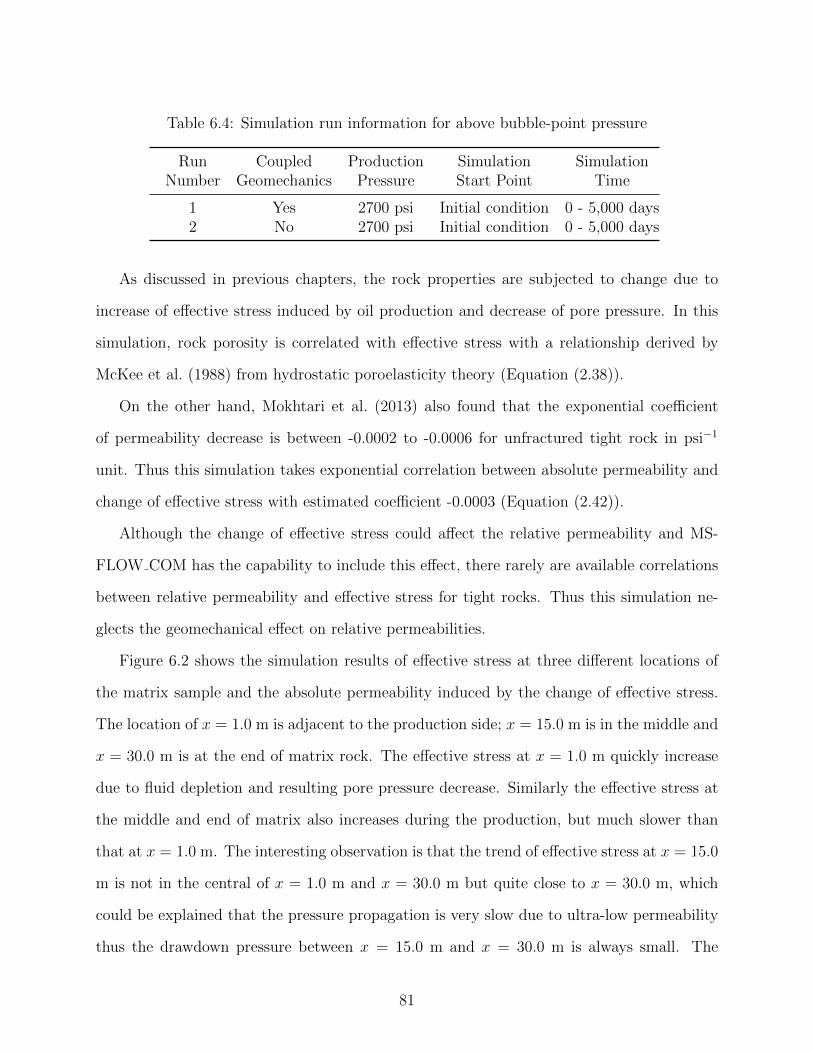
Table 6.4: Simulation run information for above bubble-point pressure
Run Coupled Production Simulation SimulationNumber Geomechanics Pressure Start Point Time
1 Yes 2700 psi Initial condition 0 - 5,000 days2 No 2700 psi Initial condition 0 - 5,000 days
As discussed in previous chapters, the rock properties are subjected to change due to
increase of effective stress induced by oil production and decrease of pore pressure. In this
simulation, rock porosity is correlated with effective stress with a relationship derived by
McKee et al. (1988) from hydrostatic poroelasticity theory (Equation (2.38)).
On the other hand, Mokhtari et al. (2013) also found that the exponential coefficient
of permeability decrease is between -0.0002 to -0.0006 for unfractured tight rock in psi−1
unit. Thus this simulation takes exponential correlation between absolute permeability and
change of effective stress with estimated coefficient -0.0003 (Equation (2.42)).
Although the change of effective stress could affect the relative permeability and MS-
FLOW COM has the capability to include this effect, there rarely are available correlations
between relative permeability and effective stress for tight rocks. Thus this simulation ne-
glects the geomechanical effect on relative permeabilities.
Figure 6.2 shows the simulation results of effective stress at three different locations of
the matrix sample and the absolute permeability induced by the change of effective stress.
The location of x = 1.0 m is adjacent to the production side; x = 15.0 m is in the middle and
x = 30.0 m is at the end of matrix rock. The effective stress at x = 1.0 m quickly increase
due to fluid depletion and resulting pore pressure decrease. Similarly the effective stress at
the middle and end of matrix also increases during the production, but much slower than
that at x = 1.0 m. The interesting observation is that the trend of effective stress at x = 15.0
m is not in the central of x = 1.0 m and x = 30.0 m but quite close to x = 30.0 m, which
could be explained that the pressure propagation is very slow due to ultra-low permeability
thus the drawdown pressure between x = 15.0 m and x = 30.0 m is always small. The
81

effect of change of effective stress on absolute permeability is shown in Figure 6.2 (b), and
the increase of effective stress is about 3000 psi (approximately from 4000 psi to 7000 psi in
Figure 6.2 (a)). The permeability evolution generally follows the trend of effective stress.
(a) Effective stress evolution (b) Permeability evolution induced by the change ofeffective stress
Figure 6.2: Effective stress evolution and induced change of permeability.
The stress-induced decrease of absolute permeability could affect the production rate.
The oil production comparison between Run1 (coupled geomechanics) and Run2 (no geome-
chanics effect) is shown in Figure 6.3 from 0 - 1000 days and 1000 - 5000 days. It shows
that Run2 has higher oil production rate than Run1 from beginning till about 1500 days
because the stress-induced permeability decease is included in Run1, and most decrease of
rock permeability occurs from beginning to about 1500 days shown in Figure 6.2 (b). The
two curves of production rate cross each other at about 1500 days shown in Figure 6.3 (b)
and Run1 has higher production rate than Run 2 since then. This is because Run1 has higher
reservoir pressure at this point due to slower production and the stress-induced decrease of
permeability tends to stabilize. Figure 6.4 presents the pressure profile at the 2000th day
and 5000th day for Run1 and Run2. It shows that Run1 has higher reservoir pressure due
to lower production rate and the pressure difference reaches largest at x = 30.0 m.
82

(a) Oil production from 0 - 1000 days (b) Oil production from 1000 - 5000 days
Figure 6.3: Comparison of oil production rate.
(a) Pressure profile at the 2000th days (b) Pressure profile at the 5000th days
Figure 6.4: Comparison of pressure profile.
83

Although Run1 has higher production from 1500 - 5000 days but the production rate
is much smaller than that at the beginning of production, the accumulated oil and gas
production of Run1 is still lower than Run2 shown in Figure 6.5. The gap between the curves
shows the difference of accumulated production between the two runs; the gap increases
from beginning to some point and then shrink, which means that the higher production rate
of Run1 after about 1500 days offsets the previously accumulated gap. The accumulated
gas production has same pattern and trend as accumulated oil production because reservoir
pressure is above saturation pressure and the producing GOR is constant to be gas solubility.
(a) Accumulated oil production (b) Accumulated gas production
Figure 6.5: Comparison of accumulated oil and gas production between Run1 and Run2.
6.2.2 Below Saturation Pressure
In this simulation study, the production pressure is further lowered from previous 2700
psi to 1500 psi, and the simulation continues from end point of Run1 and Run2 of previous
section. The gas phase quickly appears and the effects of capillary on VLE, along with rock
deformation, are studied. There are four simulation runs performed summarized in Table 6.5
in this part. The comparison study between Run2-1 and Run2-2 shows the capillary effect on
VLE and its influence on the production performance. Since rock deformation leads to the
84

change of pore radius and capillary pressure, the simulation studies on Run1-1 and Run1-2
could illustrate the influence of rock deformation on capillary pressure, therefore on VLE
and production performance.
Table 6.5: Simulation run information for below bubble point pressure
Run Coupled Capillarity Production Simulation SimulationNumber Geomechanics Effect Pressure Start Point Time (Days)
Run1-1 YES YES 1500 psi Ending state of Run1 5,000 - 15,000Run1-2 YES NO 1500 psi Ending state of Run1 5,000 - 15,000Run2-1 NO YES 1500 psi Ending state of Run2 5,000 - 15,000Run2-2 NO NO 1500 psi Ending state of Run2 5,000 - 15,000
The Young-Laplace equation (Equation (2.45)) is used to calculate the capillary pressure
between oil and gas phase by assuming contact angle is zero. The interfacial tension between
oil and gas phase is calculated with phase composition data and Parachor values of each
component with Equation (2.46). Ayirala and Rao (2006) claim that the measured interfacial
tensions are two to three times greater than those calculated with Macleod and Sugden
correlation (Equation (2.46)) at moderate pressures; Nojabaei et al. (2013) uses three times of
interfacial tension calculated with Equation (2.46) in the study of Bakken tight oil simulation.
Thus a similar correction is taken in this study to correct the underestimated interfacial
tension. The stress effect on capillary pressure is included by using the relationship between
pore radius and rock porosity and permeability with Equation (2.48); its coefficients c and
b are assumed so that the initial pore radius is about 30 nm.
6.2.2.1 Effect of Capillary Pressure on VLE
As discussed in previous chapters, the capillary pressure could postpones the appearance
of gas phase, and affect the thermodynamic properties of oil and gas phases through its effect
on VLE calculations; eventually it influences the production performance.
Figure 6.6 shows the simulation results of gas saturation at three locations of x = 1.0, 15.0
and 30.0 m. The gas saturation at all three locations is lower in Run2-1 with capillarity effect
85

on VLE. The gas saturation at x = 1.0 m quickly increases due to fluid depletion resulting
pressure decrease. It is noted that the gas saturation at x = 1.0 m reaches a peak quickly and
then decrease at beginning of production shown in Figure 6.6 (a). It’s because the formed
gas at this location flows fast to surface and there is no sufficient gas formed in rest area to
charge the gas production due to slow pressure propagation in ultra-low permeability rock.
The comparison of gas saturation at x = 15.0 and x = 30.0 m demonstrates the postponed
appearance of gas phase in Run2-1 with the effect of capillary pressure on VLE. For example,
the first gas bubble comes out at x = 15.0 at approximate 5600 day in Run2-1 and 5200 day
in Run2-2, about 400 days postpone shown in Figure 6.6(b). Similarly there is about 600
days delayed appearance of gas phase at x = 30.0 shown in Figure 6.6(c)
(a) x = 1.0 m (b) x = 15.0 m (c) x = 30.0 m
Figure 6.6: Gas saturation at three locations of Run2-1 and Run2-2.
The higher gas saturation in reservoir condition of Run2-2 could lead to more light
components transported in gas phase and therefore produced to the surface. In order to
facilitate compositional analysis, C1 and C2 components are categorized as light components;
C3, C4 and C5 − C6 are categorized as intermediate components; C7 − C12, C13 − C21 and
C22 − C80 are categorized as heavy components in the following discussions. Figure 6.7
shows the molar fraction comparison of surface production between Run2-1 and Run2-2.
It is observed that there is larger molar fraction of light components produced in the case
without capillarity effect; and Run2-1, including capillarity effect on VLE, has large molar
86

fraction of intermediate and heavy components produced.
(a) Molar fraction of C1 and C2 (b) Molar fraction of C3, C4 andC5 − C6
(c) Molar fraction ofC7 − C12,C13 − C21 and C22 − C80
Figure 6.7: Molar fraction of surface production.
Since Run2-2 has more molar fraction of light components and less molar fraction of
intermediate and heavy components produced to surface, the molar fractions in the reser-
voir condition are also difference between Run2-1 and Run2-2. Figure 6.8, Figure 6.9 and
Figure 6.10 presents the comparisons of simulation results for the overall molar fraction in
oil and gas phases at three locations of x = 1.0, 15.0 and 30.0 m. In the reservoir condition,
Run2-1, with capillarity effect on VLE, has more molar fraction of light components and less
molar fraction of intermediate and heavy components than Run2-2; because Run2-1 has less
light components and more intermediate and heavy components produced to surface shown
in Figure 6.7.
The simulated reservoir pressures of Run2-1 and Run2-2 are presented in Figure 6.11 and
Figure 6.12, respectively showing the pressure evolution at x = 1.0, 15.0 and 30.0 m, and
pressure profile of matrix rock at the 10, 000th day and the 15, 000th day. Both Figure 6.11 and
Figure 6.12 show that Run2-2, without capillarity effect on VLE, has higher reservoir pressure
than Run2-1 except at x = 1.0 m, where the pressure is very close to the production pressure.
The difference of reservoir pressure can be explained by the differences of appearance of gas
phase and corresponding gas saturation. Run2-1 has postponed appearance of gas phase and
less gas saturation, therefore faster pressure decrease. For example, the pressure of Run2-1
87
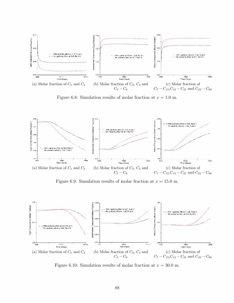
(a) Molar fraction of C1 and C2 (b) Molar fraction of C3, C4 andC5 − C6
(c) Molar fraction ofC7 − C12,C13 − C21 and C22 − C80
Figure 6.8: Simulation results of molar fraction at x = 1.0 m.
(a) Molar fraction of C1 and C2 (b) Molar fraction of C3, C4 andC5 − C6
(c) Molar fraction ofC7 − C12,C13 − C21 and C22 − C80
Figure 6.9: Simulation results of molar fraction at x = 15.0 m.
(a) Molar fraction of C1 and C2 (b) Molar fraction of C3, C4 andC5 − C6
(c) Molar fraction ofC7 − C12,C13 − C21 and C22 − C80
Figure 6.10: Simulation results of molar fraction at x = 30.0 m.
88
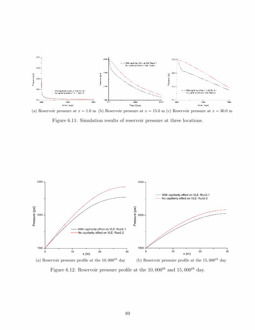
(a) Reservoir pressure at x = 1.0 m (b) Reservoir pressure at x = 15.0 m (c) Reservoir pressure at x = 30.0 m
Figure 6.11: Simulation results of reservoir pressure at three locations.
(a) Reservoir pressure profile at the 10, 000th day (b) Reservoir pressure profile at the 15, 000th day
Figure 6.12: Reservoir pressure profile at the 10, 000th and 15, 000th day.
89

at x = 30.0 m in Figure 6.11 (c) decreases much faster between approximate the 5000th and
6000th day due to no gas phase in Run2-1 and forming of gas phase in Run2-2 during this
period.
The above differences of simulation results on gas saturation, reservoir and surface com-
position, and reservoir pressure between Run2-1 and Run-2 are due to the effects of capillary
pressure between oil and gas phases on their phase equilibrium. This effect can be observed
from Figure 6.13, showing the comparison of oil phase composition at equilibrium as function
of reservoir pressure.
Before reservoir pressure decreases to the saturation pressure, Run2-1 and Run2-2 have
same and constant oil composition in reservoir condition as the overlap curves in Figure 6.13
from initial reservoir pressure to approximate 2500 psi. Once reservoir pressure decreases to
saturation pressure, the molar fraction of light components decreases, and molar fractions
of intermediate and heavy components increase. The difference of phase transition point
in Figure 6.13 shows that the saturation pressure in the case of capillarity effect on VLE is
about 200 psi lower than the case without capillarity effect. For same reservoir pressure below
bubble point, there are more light components, but less intermediate and heavy components
in oil phase due to capillarity effect on VLE.
(a) Molar fraction of C1 and C2 inoil phase
(b) Molar fraction of C3, C4 andC5 − C6 in oil phase
(c) Molar fraction ofC7 −C12,C13 −C21 and C22 −C80 in
oil phase
Figure 6.13: Oil phase composition at reservoir condition.
90

The difference of oil composition between Run2-1 and Run2-2 also leads to the difference
of fluid properties of oil phase. Figure 6.14 presents the viscosity and density of oil phase
under reservoir pressure between Run2-1 and Run2-2. It shows that Run2-1 and Run2-
2 have same oil density and viscosity above saturation pressure, and capillarity effect on
oil composition shown in Figure 6.13 leads to less density and viscosity below saturation
pressure.
(a) Oil density under reservoir pressure (b) Oil viscosity under reservoir pressure
Figure 6.14: Capillarity effect on oil density and viscosity under reservoir pressure.
The capillary pressure involved in VLE calculation is determined with Young-Laplace
Equation (2.45) and surface tension between oil and gas is evaluated with compositional
data with Equation (2.46). Figure 6.15 shows the calculated capillary pressure in simulation
Run2-1, and the range of the capillary pressure involved in VLE calculation is between 90.0
psi and 116.0 psi for this reservoir rock.
With above discussion on simulation results between Run2-1 and Run2-2, Figure 6.16
presents the effect of capillary pressure on the final production. The Run2-1, with capillarity
effect on VLE, has more accumulated oil production but less accumulated gas production
than Run2-2, due to the postponed gas phase appearance, less gas saturation, and less light
components produced. On the other hand, Run2-2 has more gas produced.
91

Figure 6.15: Capillary pressure involved in VLE calculation.
(a) Accumulated oil production (b) Accumulated gas production
Figure 6.16: Comparison of accumulated production between Run2-1 and Run2-2.
92

6.2.2.2 Geomechanical Effect
There are two main aspects of geomechanical effects on the production below saturation
pressure. The first effect is same as that on the production above saturation pressure, which
is the effect on rock permeability and porosity. Another effect is that the stress-induced
change on rock properties leads to the change of capillary pressure between oil and gas
phases and therefore affects the VLE. In other words, the effect of capillary pressure on VLE
is enhanced by the increase of effective stress during the production.
Figure 6.17 presents the oil composition as function of reservoir pressure for difference
scenarios. It shows the comparisons among three cases: no capillarity effect on VLE, with
capillarity effect on VLE only, with both capillarity and geomechanics effects. The capillary
pressure between oil and gas phases is higher for the case including geomechanics effect due
to increase of effective stress affecting pore radius. This higher capillary pressure further
suppresses saturation pressure therefore Figure 6.17 shows there more light components and
less intermediate and heavy components in oil phase than other two cases. Similarly the
oil properties, such as oil density and viscosity at reservoir conditions are also difference for
above three cases shown in Figure 6.18.
(a) Molar fraction of C1 and C2 inoil phase
(b) Molar fraction of C3, C4 andC5 − C6 in oil phase
(c) Molar fraction ofC7 −C12,C13 −C21 and C22 −C80 in
oil phase
Figure 6.17: Oil phase composition at reservoir condition.
93

(a) Oil density under reservoir pressure (b) Oil viscosity under reservoir pressure
Figure 6.18: Capillarity effect on oil density and viscosity under reservoir pressure.
The geomechanical effect leads to higher capillarity pressure, and accordingly there is
larger effect on VLE calculations, which explains the comparison in Figure 6.17 and Fig-
ure 6.18. Figure 6.19 shows the difference of capillary pressure induced by the change of
effective stress at x = 1.0, 15.0 and 30.0 m. The capillary pressure without geomechanical
effect in Run2-1 is between is between 90 and 160 psi, and it increases to between 150 and
190 psi due to stress-induced decrease of pore radius in the production above saturation
pressure (from initial state to the 5000th day).
In addition to geomechanical effect on capillary pressure, the capillarity effect on VLE
also influences the computation of effective stress. As presented in Figure 6.12 of previous
section, the reservoir pressure is different between the cases with capillarity effect on VLE and
without this effect because higher gas saturation in reservoir in the case without capillarity
effect on VLE leads to higher reservoir pressure. Consequently it affects the effective stress.
Figure 6.20 shows the comparison of simulated effective stress between Run1-1 and Run1-
2 at x = 1.0, 15.0 and 30.0 m. It shows that the case including capillarity effect on VLE has
higher effective stress due to its lower reservoir pressure shown in Figure 6.21 (a). It is noted
that the difference between reservoir pressure could reach as high as 300 psi between Run1-1
94

Figure 6.19: Capillary pressure involved in VLE calculation.
and Run1-2, much higher than the difference between Run2-1 and Run2-2 in Figure 6.12
(b) of previous section. One reason for it is that the capillarity effect on VLE in the case
with geomechanics is stronger therefore larger difference of reservoir pressure is observed in
Figure 6.21 (a) than in Figure 6.12 (b). Figure 6.21 (b) shows the profile of effective stress
for the matrix rock at the end of the simulation. Since the change of effective stress also
affects the rock properties, especially absolute permeability of tight rock, Figure 6.21 (c)
shows the profile comparison of absolute permeability between the cases whether to include
capillarity effect.
The accumulated production below saturation pressure is also compared for all the four
simulation runs shown in Figure 6.22. The accumulated production of oil and gas in the cases
with geomechanical effect, are less than the cases without geomechanical effect, because the
absolute permeability decreases due to increase of effective stress. And the capillarity effect
on VLE favors more liquid but less gas productions.
95

(a) Effective stress at x = 1.0 m (b) Effective stress at x = 15.0 m (c) Effective stress at x = 30.0 m
Figure 6.20: Simulation results of effective stress.
(a) Reservoir pressure profile (b) Effective stress profile (c) Permeability profile
Figure 6.21: Reservoir pressure, effective stress and permeability profile at end ofsimulation.
96

(a) Accumulated oil production (b) Accumulated gas production
Figure 6.22: Comparison of accumulated production.
6.2.3 Summary and Discussions
This matrix rock example illustrates how the effects of geomechanics and capillarity
on VLE influence the production performance. During the production above saturation
pressure, there is no VLE calculation required and only geomechanical effect is observed.
The increase of effective stress and consequently induced decrease of permeability leads to
less oil and gas production compared with the case without geomechanics effect.
For the production below saturation pressure, the effect of capillary pressure on VLE is
observed through compositional analysis on produced fluids and oil composition at reservoir
condition. The capillarity effect on VLE leads to suppressed saturation pressure and post-
poned appearance of gas phase. Thus there are less gas and more oil (less molar fraction of
light components and more molar fractions of intermediate and heavy components) produced
at surface due to capillarity effect. The oil composition at reservoir condition is also affected
by the suppression of saturation pressure, which leads to more light components dissolved in
oil phase, and the fluid properties, such as oil density and viscosity is accordingly influenced.
The geomechanical effect not only affect fluid flow through induced change on absolute
permeability, but also strengthen the capillarity effect due to stress-induced decrease of pore
97

radius and increase of capillary pressure. Therefore the further suppression of saturation
pressure and postponed appearance gas phase is observed in the simulations. On the other
hand, the capillarity effect on VLE in turn has impacts on the reservoir pressure and ef-
fective stress due to its influence on gas appearance and saturation. Therefore the effect of
capillary pressure on VLE and geomechanics are interlinked and affect each other during the
production below saturation pressure.
It is also noted that the increase of effective stress mainly occurs during the production
above oil saturation pressure because of very high initial pore pressure for tight oil reservoirs.
In this example, the effective stress increases about 3000 psi during the production above
saturation pressure, and about 500 psi during the production below saturation pressure. In
other words, the geomechanical effect is prominent during the production above oil saturation
pressure.
The correlation between effective stress and absolute permeability varies from rock to
rock, and a different correlation could give another simulation results. Still, the above effects
of capillary pressure and effective stress on fluid composition and production performance
exist and the corresponding analysis remains.
In addition, a tight oil reservoir usually involves multiple porous media and fractured
rocks besides tight matrix. The numerical study on the matrix rock is extended to the
following tight reservoirs with multiple porous media and fractured rocks.
98

CHAPTER 7
NUMERICAL STUDIES ON A FRACTURED RESERVOIR
The second numerical study example presented in this chapter addresses a hydraulically-
fractured horizontal well with a variety of rock types, including hydraulic fractures, natural
fractures and matrix rocks; it extends numerical studies from a single-porosity matrix, sim-
ulated in last chapter, to a multiple-porosity tight reservoirs.
7.1 A Fractured Reservoir With Double Porosity System
This section presents a tight oil reservoir with horizontal production well and multistage
hydraulic fractures. Mayerhofer et al. (2010) introduced the concept of stimulated reservoir
volume (SRV) to describe the size of created or enhanced fracture network by hydraulic
fracturing. In this simulation example, an optimal case for creating SRV is considered where
all the areas between hydraulic fractures are activated as fracture network. Figure 7.1 shows
the schematic diagram of full reservoir, including a horizontal well, three-stage hydraulic
fractures, and natural fractures within SRV and outside SRV. The natural fractures in SRV
is enhanced by hydraulic fracturing thus we distinguish the natural fractures as macro-
fractures and micro-fractures within and outside SRV.
In addition to the fractures network providing conductivity for fluid flow, the matrix
rock mainly stores the subsurface fluids. Therefore a double porosity model (Barenblatt
et al., 1960; Kazemi et al., 1976; Warren and Root, 1963) is employed in this simulation
study. In classical double porosity model, the global flow occurs only through the fracture
continuum, while the inter-porosity flow between fracture and matrix occurs locally through a
transfer function. Warren and Root (1963) introduces a ”matrix shape factor” to characterize
the local interactions between fracture and matrix. Wu and Pruess (1986) proves that the
shape factor can be accommodated with geometric parameters in the integral finite difference
99
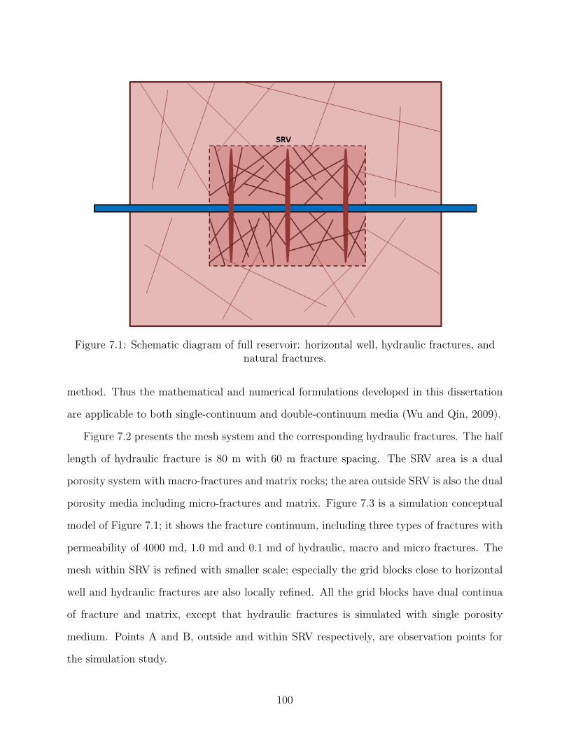
Figure 7.1: Schematic diagram of full reservoir: horizontal well, hydraulic fractures, andnatural fractures.
method. Thus the mathematical and numerical formulations developed in this dissertation
are applicable to both single-continuum and double-continuum media (Wu and Qin, 2009).
Figure 7.2 presents the mesh system and the corresponding hydraulic fractures. The half
length of hydraulic fracture is 80 m with 60 m fracture spacing. The SRV area is a dual
porosity system with macro-fractures and matrix rocks; the area outside SRV is also the dual
porosity media including micro-fractures and matrix. Figure 7.3 is a simulation conceptual
model of Figure 7.1; it shows the fracture continuum, including three types of fractures with
permeability of 4000 md, 1.0 md and 0.1 md of hydraulic, macro and micro fractures. The
mesh within SRV is refined with smaller scale; especially the grid blocks close to horizontal
well and hydraulic fractures are also locally refined. All the grid blocks have dual continua
of fracture and matrix, except that hydraulic fractures is simulated with single porosity
medium. Points A and B, outside and within SRV respectively, are observation points for
the simulation study.
100

Figure 7.2: Mesh system of hydraulic fractured reservoir.
Figure 7.3: Fracture continuum: hydraulic fracture, macro-fracture and micro-fracture.
101

The compositional data used in this simulation is same as previous example shown in
Table 6.1 and Table 6.2. The extended Brooks-Corey type of functions for three-phase flow
(Honarpour et al., 1986; Wu, 1998) is also used to model relative permeability for different
types of rocks. Table 7.1 lists the hydraulic properties of different scale of fractures and
matrix rocks.
Table 7.1: The hydraulic properties of different types of rocks
Properties Value Unit
Hydraulic fracturesPermeability 3.95× 10⁻¹² (4.0× 10³) m2 (md)Porosity 0.5
Macro-fracturesPermeability 9.87× 10⁻¹⁶ (1.0) m2 (md)Porosity 0.002
Micro-fracturesPermeability 9.87× 10⁻¹⁷ (0.1) m2 (md)Porosity 0.002
Residual saturations of fracture rockCritical gas saturation 0.01Residual water saturation 0.30Residual oil saturation 0.05
Matrix rockPermeability 2.96× 10⁻¹⁹ (3.0× 10⁻⁴) m2 (md)Porosity 0.056Critical gas saturation 0.01Residual water saturation 0.531Residual oil saturation 0.211
7.2 Geomechanical Effect
We observe that the geomechanical effect on rock properties mainly occurs during the
production above saturation pressure in Chapter 6, because there is a large pressure decrease
from initial very high reservoir pressure to oil saturation pressure. Thus the simulation study
of this section mainly focuses on the production above oil saturation pressure to analyze the
102

geomechanical effect. Table 7.2 lists the geomechanical properties of fracture and matrix
rocks in the simulation; it is noted that the fracture rock is less stiff than matrix rock with
smaller Young’s modulus, larger compressibility and Biot coefficient.
Table 7.2: The geomechanical properties of different types of rocks
Properties Value Unit
Hydraulic fracturesRock compressibility 2.85 × 10 −10 (1.97× 10⁻⁶) Pa−1 (psi−1)Young’s modulus 10 (1.45×10⁶) GPa (psi)Poisson’s ratio 0.25Biot coefficient 0.85
Natural-fracturesRock compressibility 2.45 × 10 −10 (1.69× 10⁻⁶) Pa−1 (psi−1)Young’s modulus 16 (2.32×10⁶) GPa (psi)Poisson’s ratio 0.25Biot coefficient 0.80
Matrix rockRock compressibility 1.45 × 10 −10 (1× 10⁻⁶) Pa−1 (psi−1)Young’s modulus 26 (3.77×10⁶) GPa (psi)Poisson’s ratio 0.25Biot coefficient 0.68
7.2.1 Simulation Results
The initial reservoir pressure and mean stress in this simulation is assumed to the same
as previous example, 6850 psi and 8800 psi respectively. A constant production pressure
is set to 3000 psi and 3 years simulation is performed. Two simulation runs, with and
without geomechanical effect, are compared in this section. The stress-induced permeability
change is the main factor affecting production performance discussed before. The exponential
dependency of permeability on effective stress is usually observed in a fractured tight reservoir
(Cho et al., 2013; Rutqvist et al., 2002; Wang et al., 2015); thus Equation (2.42) is used for
the correlation between absolute permeability and effective stress.
103

Figure 7.4 , Figure 7.5 and Figure 7.6 presents the evolution of permeability, effective
stress and reservoir pressure of both fracture and matrix rock at observation points, A and
B, outside and within SRV respectively. The permeability decreases due to the increases of
effective stress for both fracture and matrix rocks. The stress-induced decrease of perme-
ability within SRV mainly occurs at the early of production because of the quick decrease of
pressure in this area, especially for the fracture rock, shown in sub-figure (b) of Figure 7.4 ,
Figure 7.5 and Figure 7.6. On the other hand, a continuous stress-induced effect has been
observed for the rocks outside SRV.
(a) Permeability of matrix and fracture at A (b) Permeability of matrix and fracture at B
Figure 7.4: Stress-induced permeability change outside SRV (location A) and within SRV(location B).
The geomechanical effect on permeability is not only a function of simulation time, but
also dependent on the location. Figure 7.7 presents the permeability contour diagram of
matrix and micro-fractures after 3 years production. For both matrix and fracture rock, the
more close to hydraulic fractures or SRV, the permeability is lower due to larger pressure
decrease and corresponding larger increase of effective stress.
Figure 7.8 shows the comparison of production performance with and without geome-
chanical effect. The oil production rate is plotted in log-log scale in figure (a) due to quick
decrease of production rate in very short of time at the beginning. This shape of the oil rate
104

(a) Effective stress of matrix and fracture at A (b) Effective stress of matrix and fracture at B
Figure 7.5: Effective stress evolution outside SRV (location A) and within SRV (locationB).
(a) Reservoir pressure of matrix and fracture at A (b) Reservoir pressure of matrix and fracture at B
Figure 7.6: Reservoir pressure evolution outside SRV (location A) and within SRV(location B).
105
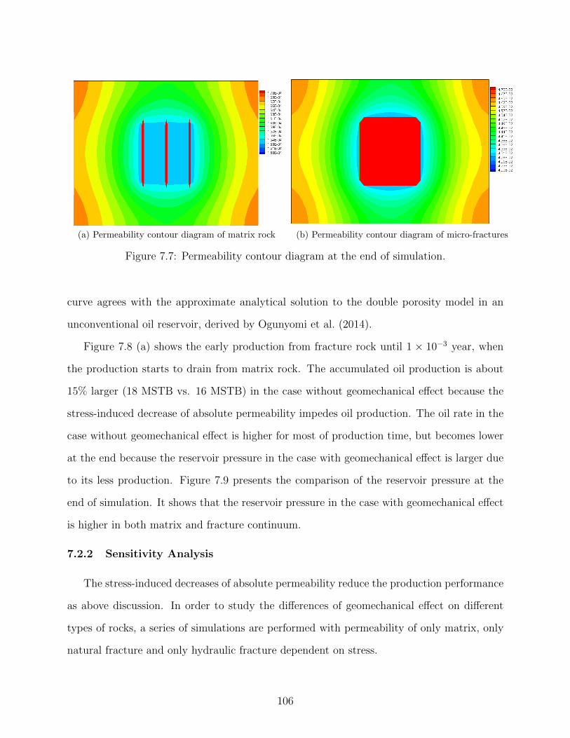
(a) Permeability contour diagram of matrix rock (b) Permeability contour diagram of micro-fractures
Figure 7.7: Permeability contour diagram at the end of simulation.
curve agrees with the approximate analytical solution to the double porosity model in an
unconventional oil reservoir, derived by Ogunyomi et al. (2014).
Figure 7.8 (a) shows the early production from fracture rock until 1 × 10⁻³ year, when
the production starts to drain from matrix rock. The accumulated oil production is about
15% larger (18 MSTB vs. 16 MSTB) in the case without geomechanical effect because the
stress-induced decrease of absolute permeability impedes oil production. The oil rate in the
case without geomechanical effect is higher for most of production time, but becomes lower
at the end because the reservoir pressure in the case with geomechanical effect is larger due
to its less production. Figure 7.9 presents the comparison of the reservoir pressure at the
end of simulation. It shows that the reservoir pressure in the case with geomechanical effect
is higher in both matrix and fracture continuum.
7.2.2 Sensitivity Analysis
The stress-induced decreases of absolute permeability reduce the production performance
as above discussion. In order to study the differences of geomechanical effect on different
types of rocks, a series of simulations are performed with permeability of only matrix, only
natural fracture and only hydraulic fracture dependent on stress.
106
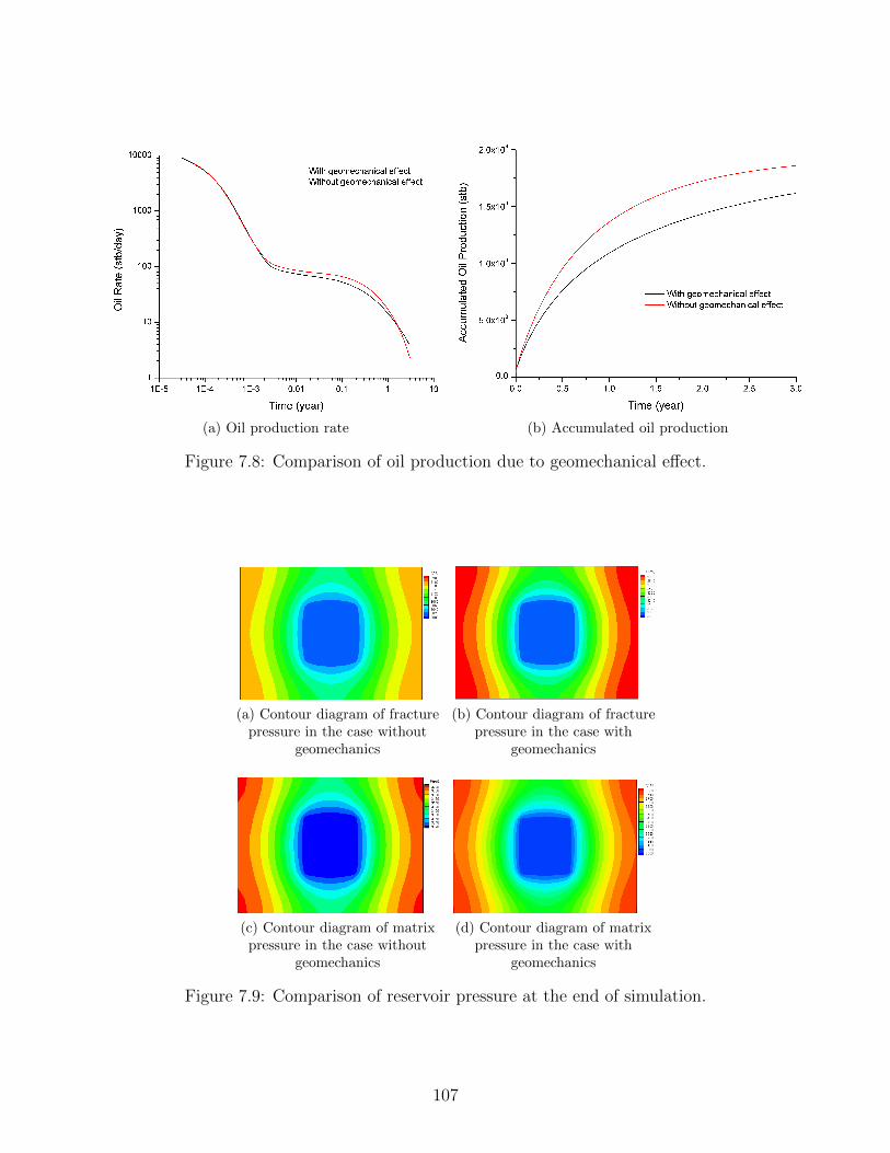
(a) Oil production rate (b) Accumulated oil production
Figure 7.8: Comparison of oil production due to geomechanical effect.
(a) Contour diagram of fracturepressure in the case without
geomechanics
(b) Contour diagram of fracturepressure in the case with
geomechanics
(c) Contour diagram of matrixpressure in the case without
geomechanics
(d) Contour diagram of matrixpressure in the case with
geomechanics
Figure 7.9: Comparison of reservoir pressure at the end of simulation.
107

(a) Oil production rate (b) Accumulated oil production
Figure 7.10: Sensitivity analysis of geomechanical effects of different rocks.
Figure 7.10 shows the production performance for the scenarios: (1) without geomechan-
ical effect; (2) only permeability of natural fracture, kf , is dependent on stress (permeability
of matrix and hydraulic fractures are not stress-dependent); (3) only permeability of ma-
trix, km, is dependent on stress (permeability of natural fracture and hydraulic fracture are
not stress-dependent);(4)only permeability of hydraulic fracture, kHF is dependent on stress
(permeability of matrix and natural fracture are not stress-dependent); (5) permeability of
all rocks are stress-dependent. From Figure 7.10, the accumulation production of scenario
(2) is most close to scenario (5), and scenario (4) is most close to scenario (1). It means that
the stress effect on natural fractures has the most influence on the production performance,
and the stress effect on the hydraulic fractures has the least influence.
7.3 Effect of Capillary Pressure
Since the effect of capillary pressure only exists during the production with reservoir
pressure below saturation pressure, a constant production pressure is set to 1500 psi, below
saturation pressure, in this simulation. It is also assumed the reservoir has been depleted
for some time; the current pressure (initial pressure of this simulation) is 3000 psi. A total
108

60 years simulation is performed in this study so that the reservoir is fully drained at 1500
psi production pressure.
Two simulation runs, with and without effect of capillary pressure on VLE, are performed
and the simulation results are compared in this section. The range of the capillary pressure
is similar to previous simulation example shown in Figure 6.19. And the effect of capillary
pressure on VLE is only considered for matrix rocks because of very small capillary pressure
in fracture continuum due to its large pore space.
7.3.1 Simulation Results
At the very beginning of the simulation, the depletions are mainly from fracture con-
tinuum and thus the effect of capillary pressure on the flow behaviors cannot be observed.
Figure 7.11 and Figure 7.12 shows the pressure and gas saturation contour diagram of frac-
ture system after 1 day simulation, and there is no noticeable differences observed between
the simulation runs with and without capillarity effect.
(a) Pressure contour diagram without capillarity effect (b) Pressure contour diagram with capillarity effect
Figure 7.11: Pressure contour diagram of Day 1 in fracture continuum.
The figures also show that the fluid drainage barely reaches the fracture system outside
SRV, where the reservoir pressure is almost same as initial and there is no gas phase formed.
Accordingly the matrix continuum is almost not depleted at all at this moment (Day 1),
with the same condition as initial state.
109

(a) Gas saturation contour diagram without capillarityeffect
(b) Gas saturation contour diagram with capillarityeffect
Figure 7.12: Gas contour diagram of Day 1 in fracture continuum.
The capillary effect is observed as the production continues and reservoir pressure, es-
pecially matrix pressure decreases below saturation pressure. One of the main observed
characteristics in the simulation runs with capillarity effect is the lower reservoir gas satura-
tion due to suppressed saturation pressure. For example, Figure 7.13 presents the comparison
of gas saturation at the end of 10 years simulation in both fracture and matrix system.
The difference in gas saturation also leads to the other differences, such as reservoir
pressure. Figure 7.14 shows the comparison of reservoir pressure after 10 years’ production
in the cases with and without capillarity effect. It shows that the reservoir pressure of both
matrix and fracture system is higher in the case without capillary effect at this moment.
The differences of gas saturation in both fracture and matrix systems are observed
throughout the whole 60 years simulation. Figure 7.15 shows the gas saturation contour
diagram at the end of the simulation, where the gas saturation in the case without capillar-
ity effect is about 0.02 higher in both fracture and matrix systems.
The simulation results at observation locations A (outside SRV) and B (inside SRV) in
Figure 7.2 are also plotted below to further demonstrate the capillarity effect. Figure 7.16
and Figure 7.17 shows the comparison of simulation results at location A and B respectively.
110

(a) Gas saturation contour diagram without capillarityeffect in matrix system
(b) Gas saturation contour diagram with capillarityeffect in matrix system
(c) Gas saturation contour diagram without capillarityeffect in fracture system
(d) Gas saturation contour diagram with capillarityeffect of fracture system
Figure 7.13: Gas saturation contour diagram after 10 years in both matrix and fracturecontinuum (left: without capillarity effect; right: with capillarity effect; top: matrix
system; bottom: fracture system).
111

(a) Reservoir pressure contour diagram withoutcapillarity effect in matrix system
(b) Reservoir pressure contour diagram with capillarityeffect in matrix system
(c) Reservoir pressure contour diagram withoutcapillarity effect in fracture system
(d) Reservoir pressure contour diagram with capillarityeffect in fracture system
Figure 7.14: Reservoir pressure contour diagram after 10 years in both matrix and fracturecontinuum (left: without capillarity effect; right: with capillarity effect; top: matrix
system; bottom: fracture system).
112

(a) Gas saturation contour diagram without capillarityeffect in matrix system
(b) Gas saturation contour diagram with capillarityeffect in matrix system
(c) Gas saturation contour diagram without capillarityeffect in fracture system
(d) Gas saturation contour diagram with capillarityeffect in fracture system
Figure 7.15: Gas saturation contour diagram after 60 years in both matrix and fracturecontinuum (left: without capillarity effect; right: with capillarity effect; top: matrix
system; bottom: fracture system).
113

The differences of simulation results in fracture continuum and matrix continuum are
both observed in the two observation points in Figure 7.16 and Figure 7.17. The reservoir
pressure of fracture and matrix rocks in location A follows a similar trend in Figure 7.16
(a) and (b); the pressure in the case with capillarity effect decreases much faster at the
beginning because of delayed generation of gas phase in the matrix rock in Figure 7.16 (d),
which shows about 1.5 years postpone on gas phase appearance under the effect of capillary
pressure. The gas saturation of matrix rock clearly illustrates the capillarity effect that the
gas saturation is always higher in the case without capillarity effect. Since the capillary
pressure has no effect on fracture continuum, we observe a higher gas saturation in fracture
continuum in the case with capillarity effect due to the faster decrease of reservoir pressure
in Figure 7.16 (c).
For the location within SRV, the fracture pressure quickly decrease and reach the pro-
duction pressure due to higher permeability, shown in Figure 7.17 (a). Similarly the matrix
pressure in the case with capillarity effect decrease faster at the beginning, and the matrix
pressure in SRV reaches 1500 psi after 10 years production in Figure 7.17 (b). Figure 7.17
(c) shows the gas saturation of fracture continuum within SRV; the gas saturation increases
immediately after production because of fast decrease of fracture pressure, and then deceases
to some point mainly because the gas is produced to surface and there is no sufficient gas
formed in its matrix rock in a short period of time. Again the matrix gas saturation in
Figure 7.17 (d) shows the influences of capillary pressure on gas saturation, where a lower
gas saturation is observed in the case with capillarity effect.
The overall composition and the composition of oil phase are also analyzed at the end
of simulation. The reservoir is almost fully depleted in both cases where the final reservoir
pressure is almost same, close to production pressure 1500 psi. Figure 7.18 presents the
overall composition after 60 years production; it shows that there are less light components
left in reservoir in the case without capillarity effect; because there is more light components
produced. Those light components with higher overall molar fraction are actually dissolved
114

(a) Fracture pressure (b) Matrix pressure
(c) Fracture gas saturation (d) Matrix gas saturation
Figure 7.16: Comparison of simulation results at location A (outside SRV).
115

(a) Fracture pressure (b) Matrix pressure
(c) Fracture gas saturation (d) Matrix gas saturation
Figure 7.17: Comparison of simulation results at location B (within SRV).
116
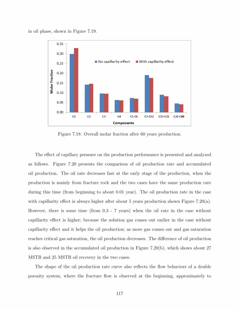
in oil phase, shown in Figure 7.19.
Figure 7.18: Overall molar fraction after 60 years production.
The effect of capillary pressure on the production performance is presented and analyzed
as follows. Figure 7.20 presents the comparison of oil production rate and accumulated
oil production. The oil rate decreases fast at the early stage of the production, when the
production is mainly from fracture rock and the two cases have the same production rate
during this time (from beginning to about 0.01 year). The oil production rate in the case
with capillarity effect is always higher after about 5 years production shown Figure 7.20(a).
However, there is some time (from 0.3 - 7 years) when the oil rate in the case without
capillarity effect is higher; because the solution gas comes out earlier in the case without
capillarity effect and it helps the oil production; as more gas comes out and gas saturation
reaches critical gas saturation, the oil production decreases. The difference of oil production
is also observed in the accumulated oil production in Figure 7.20(b), which shows about 27
MSTB and 25 MSTB oil recovery in the two cases.
The shape of the oil production rate curve also reflects the flow behaviors of a double
porosity system, where the fracture flow is observed at the beginning, approximately to
117

Figure 7.19: Molar fraction in oil phase after 60 years production.
(a) Oil production rate (b) Accumulated oil production
Figure 7.20: Comparison of oil production.
118

about 0.02 year when the oil rate decreases to a local bottom; the oil flow rate increases then
due to starting production from matrix rock, and finally decreases. This shape also matches
the approximate analytical solution to the double porosity model in an unconventional oil
reservoir, derived by Ogunyomi et al. (2014).
Figure 7.21 presents the accumulated gas production and producing gas oil ratio. It
clearly shows that there are much more gas produced in the case without capillarity effect,
89 MMSCF compared 67 MMSCF. It is also noted that the gas oil ratio at very early time
increases to about 7000 scf/stb and then quickly decreases to about 1500 scf/stb before
steadily increases, which is due to the early production from fracture rocks.
(a) Accumulated gas production (b) Producing gas oil ratio
Figure 7.21: Comparison of gas production.
7.3.2 Sensitivity Analysis
In the previous examples, the value of capillary pressure between oil and gas phases is
estimated with Young-Laplace equation (Equation (2.45)); the interfacial tension is calcu-
lated with Macleod-Sugden correlation (Equation (2.46)); the pore radius is estimated from
permeability and porosity with Equation (2.48). However, those correlations may not be
accurate for tight oil reservoirs. For example, Nojabaei et al. (2013) claims the interfacial
119

tension calculated from Macleod-Sugden correlation is two to three times lower than real
value for Bakken reservoirs; and currently there is no reliable experimental results to deter-
mine the coefficients of Equation (2.48) for tight reservoir rock. Thus it’s hard to obtain
an accurate value of capillary pressure. In this section, the capillary pressure used in the
example is scaled up 1.5 times to compare the production performance.
(a) Oil production rate (b) Accumulated oil production
(c) Accumulated gas production (d) Producing gas oil ratio
Figure 7.22: Sensitivity study of capillarity effect on production performance.
Figure 7.22 presents the results of sensitivity study of capillary effect on production
performance. With higher capillary pressure on VLE, the oil production rate and final oil
120

recovery increase but not significantly (from 26.8 MSTB to 27.2 MSTB ); on the other hand,
it has a prominent influence on the restriction of gas production (from 67 MMSCF to 60
MMSCF).
7.4 Summary and Discussions
This chapter presents a hydraulically fractured tight reservoir with two types of natural
fractures, macro-fractures within SRV and micro-fractures outside SRV, both connected to
matrix rocks. The numerical simulations involving double-porosity are performed to study
the influences on production performance due to geomechanical effect and the capillarity
effect on VLE respectively.
The geomechanical effect is modeled mainly through the stress-induced permeability
decrease. The degradation of fracture permeability is much faster than matrix permeability
within SRV, and the permeability of fracture and matrix outside SRV follows a similar
trend of degradation. Also the decrease of permeability in the areas close to SRV is more
prominent than the distant areas. The sensitivity study found that the stress-dependency of
natural fractures plays significant role on the production performance; and the stress-induced
permeability decrease for matrix rocks and hydraulic fractures has less impact on the final
production.
The capillarity effect on VLE influences the production when the reservoir pressure re-
duces below saturation pressure. At the very early of production, there is no differences
observed between the cases with and without capillarity effect on VLE, because the pro-
duction from fractures dominate the early production, and capillarity effect is negligible in
fracture continuum.
Similarly to the matrix rocks in Chapter 6, there is less gas saturation at reservoir con-
dition in the case with capillarity effect on VLE, which leads to 30% less gas and 10 % more
oil produced than the case without capillarity effect on VLE. In addition, the overall com-
position and the composition of oil phase are also different at the end of simulation in the
two cases. The sensitivity study found that the increase of the capillarity pressure effect on
121

VLE has larger influence on suppression of gas production than on growth of oil production
in this simulation case.
122
CHAPTER 8
CONCLUSIONS AND RECOMMENDATIONS
This chapter summarizes the research results of this dissertation with a number of con-
clusions and recommendations made at the end.
8.1 Summary and Contributions
This dissertation documents the development of a compositional model fully coupled
with geomechanics, from physical processes, mathematical model, to numerical formulation
and solution, for simulation of multiphase, multi-component fluid flow behaviors in tight
oil reservoirs. The geomechanical formulation is derived from the theory of poro-elasticity
with mean stress as additional primary variable. The VLE calculation in the compositional
model includes the effect of capillary pressure variation from rock deformation, which is
considered as the key to represent nano-pore confinement effect. The primary variables
selected in this compositional model are independent from VLE calculation, which gives the
flexibility to improve or change VLE calculation itself without affecting other parts of the
model. The developed simulation program, MSFLOW COM, is thoroughly validated against
experimental results, analytical solutions, and results from a commercial simulator. Thus
the following contributions are made from the developed model and numerical studies:
1. The effects of pore confinement and rock compaction on production performance of
tight oil reservoirs are qualitatively investigated. The pore confinement effect is repre-
sented with the capillarity effect on VLE, and rock compaction effect is captured with
a fully coupled mean stress model.
2. The geomechanical effect is fully coupled with fluid flow and mass transport. The fully
coupling method is numerically stable to solve flow and stress equations simultaneously
123

within each iteration, and it can be generally applied to model flow processes in stress-
sensitive petroleum reservoirs.
3. The VLE calculation includes the pore confinement effect. The nano-pore confinement
effect is captured in VLE calculation by including the capillary pressure influences on
phase equilibrium. The method of VLE calculation in this dissertation can be generally
applied to study other nano-pore confinement phenomena, such as gas condensate
systems in liquid-rich shale reservoirs.
4. The interaction between geomechanics and capillarity effect on VLE is accounted for in
the model. The stress-induced reduction of pore size results in the change of capillary
pressure and further affects the VLE. On the other hand, the capillarity effect on VLE
influences both fluid flow and effective stress. This two-way interaction process can be
rigorously modeled in this dissertation.
5. The simulator developed has the capabilities to model the complex multiphase, multi-
component fluid flow in tight oil reservoirs. The current simulation practices for tight
oil reservoirs take over-simplified approximations to describe pore confinement effect by
adjusting saturation pressure and PVT properties. This limitation is removed in this
dissertation by the compositional model with VLE calculation under rock deformation
in the in-situ fluid system at reservoir condition.
8.2 Conclusions
Two numerical examples are studied with MSFLOW COM in this dissertation, includ-
ing a single-porosity porous medium rock and a double-porosity fractured reservoir. The
following conclusions can be drawn from the simulation results and sensitivity analysis:
1. The oil production from low permeability, tight reservoirs with very high initial pore
pressure leads to substantial increase of effective stress; consequently the induced de-
crease in absolute permeability undermines the production performance.
124
2. The geomechanical effect on natural fractures has more significant impacts on the
production performance from tight, naturally fractured reservoirs than its effect on
hydraulic fractures and porous medium rocks.
3. The geomechanical effect is more prominent during the production in undersaturated
condition or with reservoir pressure above oil saturation pressure than in saturated
condition, because pore pressure decreases fast without gas phase presence at reservoir
condition and the decrease in pressure is substantial due to very high initial pressure
as well as low rock permeability.
4. The effect of capillary pressure on VLE suppresses the saturation pressure and results in
more light components dissolved in the oil phase, which influences the oil properties,
such as density and viscosity. This effect could be exaggerated due to production-
induced increase of effective stress.
5. The effect of capillary pressure on VLE leads to lower gas saturation at reservoir con-
dition, less gas and more oil production, and larger molar fraction of light components
remained in reservoir.
6. The effect of capillary pressure on VLE also leads to the different evolution of reservoir
pressure during the production, compared to the case without this effect. Reservoir
pressure decreases a little faster in the case with capillarity effect on VLE due to
postponed gas phase appearance and lower gas saturation. This evolution difference
in reservoir pressure could influence the effective stress.
8.3 Recommendations
The following recommendations are proposed for the future work based on the current
work conducted in this dissertation:
1. MSFLOW COM can be applied not only to tight oil reservoir (bubble-point system)
simulation, but also to other scenarios involving compositional modeling and/or rock
125

compaction. For example, it can be applied to study the dew point system of liquid-rich
shale reservoirs with the effects of pore confinement and stress-dependency.
2. The computational efficiency for the compositional model could be an issue to apply
MSFLOW COM for large scale reservoir simulations. In addition to the linear solver,
another big computational cost of MSFLOW COM is the Jacobian matrix assembly.
Because each derivative of Jacobian matrix is calculated with numerical differentiation
method, which requires the VLE calculation for each increment of each primary variable
of each grid block. Therefore there are many VLE calculation tasks involved in the
numerical differentiation, and VLE calculation itself is computationally costly.
Analytical solution to calculate derivatives is not recommended because its complexity
and the advantages of numerical differentiation, such as robustness and simplicity. One
recommendation is to parallelize the Jacobian matrix assembly so that the numerical
differentiation for different grid blocks can be performed simultaneously on different
processors. Another recommendation is to build a comprehensive composition data
base for a specific multi-component system beforehand, and the interpolation from the
data base could get the approximate VLE results during the simulation.
3. The numerical studies show that the effect of capillary pressure on VLE has non-
negligible influence on the production performance. However, the reliable model or
experiment data for capillary pressure in nano-pores are seldom available. Thus it is
recommended that more experimental and theoretical work should be pursued to build
an accurate model to predict or correlate the capillary pressure in nano-pores.
4. The geomechanical model of MSFLOW COM couples the mean normal stress with pore
pressure. This coupling approach has the advantages of less computational workload
and easier fully coupling with flow equations. It is rigorous and sufficient to model
the rock compaction effect in flow-focused reservoir simulations. But it is unable to
analyze shear stress related scenarios or strongly anisotropic reservoirs. In order to
126

analyze and simulate more complex stress-induced phenomena, a more comprehensive
geomechanical model is required.
127

REFERENCES CITED
Abousleiman, Y., Cheng, A.D., Cui, L. et al. 1996. Mandel’s problem revisited. Geotech-nique 46(2), 187–195.
Ahmed, T. 2006. Reservoir engineering handbook (Third ed.). Gulf Professional Publishing.
Ahmed, T. and McKinney, P. 2011. Advanced reservoir engineering. Gulf ProfessionalPublishing.
Ayirala, S.C. and Rao, D.N. 2006. A new mechanistic parachor model to predict dynamicinterfacial tension and miscibility in multicomponent hydrocarbon systems. Journal ofcolloid and interface science 299(1), 321–331.
Aziz, K. and Settari, A. 1979. Petroleum reservoir simulation, Volume 476. Applied SciencePublishers London.
Barenblatt, G., Zheltov, I.P., and Kochina, I. 1960. Basic concepts in the theory of seepageof homogeneous liquids in fissured rocks [strata]. Journal of applied mathematics andmechanics 24(5), 1286–1303.
Biot, M.A. 1957. The elastic coefficients of the theory of consolidation. J. appl. Mech. 24,594–601.
Buckley, S. and Leverett, M. 1941. Mechanism of fluid displacement in sands. Trans.Aime 146.
Cao, H. 2002. Development of techniques for general purpose simulators. Ph. D. thesis,Stanford University, Stanford, California.
Cho, Y., Ozkan, E., and Apaydin, O.G. 2013. Pressure-dependent natural-fracture perme-ability in shale and its effect on shale-gas well production. SPE Reservoir Evaluation &Engineering 16(02), 216–228. SPE–159801–PA. http://dx.doi.org/10.2118/159801-PA.
Chu, L., Ye, P., Harmawan, I.S. et al. 2012. Characterizing and simulating thenonstationariness and nonlinearity in unconventional oil reservoirs: Bakken appli-cation. In SPE Canadian Unconventional Resources Conference. Calgary, Alberta,Canada, 30 October-1 November. Society of Petroleum Engineers. SPE-161137-MS.http://dx.doi.org/10.2118/161137-MS.
128

CMG 2012. User’s guide of GEM - advanced compositional and unconventional reservoirsimulator. Computer Modeling Group Ltd., Calgary, Alberta.
Coats, K.H. 1980. An equation of state compositional model. SPE J 20(5), 363–376. SPE–8284–PA. http://dx.doi.org/10.2118/8284-PA.
Collins, D., Nghiem, L., Li, Y.K. et al. 1992. An efficient approach to adaptive-implicitcompositional simulation with an equation of state. SPE reservoir engineering 7(2), 259–264. SPE–15133–PA. http://dx.doi.org/10.2118/15133-PA.
Craft, B., Hawkins, M., and Terry, R. 1991. Applied petroleum reservoir engineering. OldTappan, NJ; Prentice Hall Inc.
Cryer, C. 1963. A comparison of the three-dimensional consolidation theories of biot andterzaghi. The Quarterly Journal of Mechanics and Applied Mathematics 16(4), 401–412.
Dabbous, M., Reznik, A., Mody, B. et al. 1976. Gas-water capillary pressure in coal atvarious overburden pressures. Society of Petroleum Engineers Journal 16(05), 261–268.SPE–5348–PA. http://dx.doi.org/10.2118/5348-PA.
Dabbous, M., Reznik, A., Taber, J. et al. 1974. The permeability of coal to gasand water. Society of Petroleum Engineers Journal 14(06), 563–572. SPE–4711–A.http://dx.doi.org/10.2118/4711-A.
Danesh, A. 1998. PVT and phase behaviour of petroleum reservoir fluids, Volume 47. Else-vier.
Davies, J. and Davies, D. 2001. Stress-dependent permeability: characterization and model-ing. SPE Journal 6(02), 224–235. SPE–71750–PA. http://dx.doi.org/10.2118/71750-PA.
Dean, R.H., Gai, X., Stone, C.M. et al. 2006. A comparison of techniques forcoupling porous flow and geomechanics. SPE Journal 11(1), 132. SPE–79709–PA.http://dx.doi.org/10.2118/79709-PA.
Deloitte 2014. Play summaries of key north american unconventional shale and canadiancoal bed methane basins. Accessed: 2014-10-06.
Dourson, R., Sage, B., and Lacey, W. 1943. Phase behavior in the Methane-Propane-n-Pentane system. Transactions of the AIME 151(01), 206–215.
Du, L. and Chu, L. 2012. Understanding anomalous phase behavior in unconventionaloil reservoirs. In SPE Canadian Unconventional Resources Conference. Calgary, Al-berta, Canada, 30 October-1 November. Society of Petroleum Engineers. SPE-161830-MS.http://dx.doi.org/10.2118/161830-MS.
129
EIA. 2013a. Annual energy outlook 2013. US Energy Information Administration, Wash-ington, DC .
EIA. 2013b. Technically recoverable shale oil and shale gas resources: an assessment of 137shale formations in 41 countries outside the united states. US Department of Energy/EIA,Washington, DC .
EIA. 2014a. Annual energy outlook 2014. US Energy Information Administration, Wash-ington, DC .
EIA. 2014b. How much oil is consumed in the united states? http://www.eia.gov/tools/faqs/faq.cfm?id=33&t=6. Accessed: 2014-10-02.
Ertekin, T., Abou-Kassem, J.H., and King, G.R. 2001. Basic applied reservoir simulation.Richardson, TX: Society of Petroleum Engineers.
Fakcharoenphol, P. 2013. A coupled flow and geomechanics model for enhanced oil and gasrecovery in shale formations. Ph. D. thesis, Colorado School of Mines, Golden, Colorado.
Fatt, I. and Davis, D. 1952. Reduction in permeability with overburden pressure. Journalof Petroleum Technology 4(12), 16. SPE–952329–G. http://dx.doi.org/10.2118/952329-G.
Firincioglu, T., Ozkan, E., and Ozgen, C. 2012. Thermodynamics of multiphase flow inunconventional liquids-rich reservoirs. In SPE Annual Technical Conference and Exhibi-tion. San Antonio, Texas, 8-10 October. Society of Petroleum Engineers. SPE-159869-MS.http://dx.doi.org/10.2118/159869-MS.
Firoozabadi, A. and Katz, D.L. 1988. Surface tension of reservoir crude-oil/gas systemsrecognizing the Asphalt in the heavy fraction. SPE Reservoir Engineering 3(01), 265–272. SPE–13826–PA. http://dx.doi.org/10.2118/13826-PA.
Gutierrez, M., Lewis, R., and Masters, I. 2001. Petroleum reservoir simulation couplingfluid flow and geomechanics. SPE Reservoir Evaluation & Engineering 4(03), 164–172.SPE–72095–PA. http://dx.doi.org/10.2118/72095-PA.
Han, G., Gutierrez, M., and Schmitz, P. 2013. Stress-dependent flow mechanical and acousticproperties for an unconventional oil reservoir rock. In Unconventional Resources Technol-ogy Conference. Denver, Colorado, 12-14 August. Society of Petroleum Engineers. SPE-168680-MS. http://dx.doi.org/10.1190/URTEC2013-177.
He, J. and Ling, K. 2014. A new method to determine Biot coefficients of Bakken samples. In48th US Rock Mechanics/Geomechanics Symposium. Minneapolis, Minnesota, 1-4 June.American Rock Mechanics Association.
130

Honarpour, M., Koederitz, F., and Herbert, A. 1986. Relative permeability of petroleumreservoirs. CRC Press Inc, Boca Raton, FL.
Honarpour, M.M., Nagarajan, N.R., Orangi, A. et al. 2012. Characterization of critical fluidPVT rock and rock-fluid properties-impact on reservoir performance of liquid rich shales.In SPE Annual Technical Conference and Exhibition. San Antonio, Texas, 8-10 October.Society of Petroleum Engineers. SPE-158042-MS. http://dx.doi.org/10.2118/158042-MS.
Hu, L., Winterfeld, P.H., Fakcharoenphol P. et al. 2013. A novel fully-coupled flow andgeomechanics model in enhanced geothermal reservoirs. Journal of Petroleum Science andEngineering 107, 1–11.
Jaeger, J.C., Cook, N.G. , and Zimmerman, R. 2007. Fundamentals of rock mechanics(Fourth ed.). John Wiley & Sons.
Jones, F.O. and Owens, W. 1980. A laboratory study of low-permeabilitygas sands. Journal of Petroleum Technology 32(09), 1631–1640. SPE–7551–PA.http://dx.doi.org/10.2118/7551-PA.
Kazemi, H., Merrill Jr, L., Porterfield, K. et al. 1976. Numerical simulation of water-oil flowin naturally fractured reservoirs. Society of Petroleum Engineers Journal 16(06), 317–326.SPE–5719–PA. http://dx.doi.org/10.2118/5719-PA.
Klinkenberg, L. 1941. The permeability of porous media to liquids and gases. In Drillingand production practice. New York, New York, 1 January. American Petroleum Institute.
Kuila, U. and Prasad, M. 2011. Understanding pore-structure and permeability in shales. InSPE Annual Technical Conference and Exhibition. Denver, Colorado, 30 October-2 Novem-ber. Society of Petroleum Engineers. SPE-146869-MS. http://dx.doi.org/10.2118/146869-MS.
Kurtoglu, B., Kazemi, H., Rosen, R. et al. 2014. A rock and fluid study of middleBakken formation: key to enhanced oil recovery. In SPE/CSUR Unconventional Re-sources Conference–Canada. Calgary, Alberta, Canada, 30 September2 October. Societyof Petroleum Engineers. SPE-171668-MS. http://dx.doi.org/10.2118/171668-MS.
Lai, B. and Miskimins, J.L. 2010. A new technique for accurately measuring two-phaserelative permeability under non-Darcy flow conditions. In SPE Annual Technical Con-ference and Exhibition. Florence, Italy, 19-22 September. Society of Petroleum Engineers.SPE-134501-MS. http://dx.doi.org/10.2118/134501-MS.
Lei, G., Dong, P., Wu, Z. et al. 2015. A fractal model for the stress-dependent permeabilityand relative permeability in tight sandstones. Journal of Canadian Petroleum Technol-ogy 54(01), 36–48. SPE–173897–PA. http://dx.doi.org/10.2118/173897-PA.
131

Leverett, M. 1940. Capillary behavior in porous solids. Trans. Am. Inst 142(01), 152–169.
Lohrenz, J., Bray, B.G. , and Clark, C.R. 1964. Calculating viscosities of reservoir fluids fromtheir compositions. Journal of Petroleum Technology 16(10), 1171–1176. SPE–915–PA.http://dx.doi.org/10.2118/915-PA.
Luneau, B., Longman, M., Kaufman, P. et al. 2011. Stratigraphy and petrophysical charac-teristics of the Niobrara formation in the Denver basin, Colorado and Wyoming. Searchand Discovery Article (50469).
Mayerhofer, M.J., Lolon, E., Warpinski, N.R. et al. 2010. What is stimulated reser-voir volume? SPE Production and Operations 25(1), 89–98. SPE–119890–PA.http://dx.doi.org/10.2118/119890-PA.
McKee, C., Bumb, A., and Koenig, R. 1988. Stress-dependent permeability and porosity ofcoal and other geologic formations. SPE formation evaluation 3(01), 81–91. SPE–12858–PA. http://dx.doi.org/10.2118/12858-PA.
Minkoff, S.E., Stone, C.M., Bryant, S. et al. 2003. Coupled fluid flow and geomechanicaldeformation modeling. Journal of Petroleum Science and Engineering 38(1), 37–56.
Mokhtari, M., Alqahtani, A.A., Tutuncu A.N. et al. 2013. Stress-dependent permeabil-ity anisotropy and wettability of shale resources. In Unconventional Resources Technol-ogy Conference. Denver, Colorado, 12-14 August. Society of Petroleum Engineers. SPE-168672-MS. http://dx.doi.org/10.1190/URTEC2013-283.
Narasimhan, T. and Witherspoon, P. 1976. An integrated finite difference method for ana-lyzing fluid flow in porous media. Water Resources Research 12(1), 57–64.
Nelson, P.H. 1994. Permeability-porosity relationships in sedimentary rocks. The log ana-lyst 35(03), 38–62.
Nelson, P.H. 2005. Permeability, porosity, and pore-throat size-: A three-dimensional per-spective. Petrophysics 46(6), 452–455.
Nelson, P.H. 2009. Pore-throat sizes in sandstones, tight sandstones, and shales. AAPGbulletin 93(3), 329–340.
Nojabaei, B., Johns, R.T., and Chu, L. 2013. Effect of capillary pressure on phase behaviorin tight rocks and shales. SPE Reservoir Evaluation & Engineering 16(03), 281–289.SPE–159258–PA. http://dx.doi.org/10.2118/159258-PA.
NRCan 2014. North American tight light oil. http://www.nrcan.gc.ca/energy/crude-petroleum/4559#oil1. Accessed: 2014-10-06.
132

Ogunyomi, B.A., Patzek, T.W. , Lake, L.W. et al. 2014. History matching and rate forecast-ing in unconventional oil reservoirs using an approximate analytical solution to the doubleporosity model. In SPE Eastern Regional Meeting. Charleston, WV, 21-23 October. Soci-ety of Petroleum Engineers. SPE-171031-MS. http://dx.doi.org/10.2118/171031-MS.
Orangi, A., Nagarajan, N.R., Honarpour, M.M. et al. 2011. Unconventional shale oil andgas-condensate reservoir production impact of rock fluid and hydraulic fractures. In SPEHydraulic Fracturing Technology Conference. The Woodlands, Texas. Society of PetroleumEngineers. SPE-140536-MS. http://dx.doi.org/10.2118/140536-MS.
Ostensen, R. 1986. The effect of stress-dependent permeability on gas produc-tion and well testing. SPE Formation Evaluation 1(03), 227–235. SPE–11220–PA.http://dx.doi.org/10.2118/11220-PA.
Pan, F. 2009. Development and application of a coupled geomechanics model for a parallelcompositional reservoir simulator. Ph. D. thesis, The University of Texas at Austin,Austin, Texas.
Peng, D.Y. and Robinson, D.B. 1976. A new two-constant equation of state. Industrial &Engineering Chemistry Fundamentals 15(1), 59–64.
Pioneer Natural Resource Inc. 2013. Horizontal spraberry/wolfcamp acceleration. In HartEnergy 2013 DUG Conference.
Pruess, K. 1991. TOUGH2: A general-purpose numerical simulator for multiphase fluid andheat flow. Technical report, Lawrence Berkeley Lab., CA.
Rachford Jr, H. and Rice, J. 1952. Procedure for use of electronic digital computers in calcu-lating flash vaporization hydrocarbon equilibrium. Journal of Petroleum Technology 4(10),327–328. SPE–952327–G. http://dx.doi.org/10.2118/952327-G.
Reyes, L. and Osisanya, S. 2002. Empirical correlation of effective stress dependent shalerock properties. Journal of Canadian Petroleum Technology 41(12), 47–53. PETSOC–02–12–02. http://dx.doi.org/10.2118/02-12-02.
Rutqvist, J., Wu, Y.S., Tsang, C.F. et al. 2002. A modeling approach for analysis of coupledmultiphase fluid flow, heat transfer, and deformation in fractured porous rock. Interna-tional Journal of Rock Mechanics and Mining Sciences 39(4), 429–442.
Santos, L. O. S. 2013. Development of a multi-formulation compositional simulator. Ph. D.thesis, The University of Texas at Austin, Austin, Texas.
133

Settari, A. and Walters, D.A. 2001. Advances in coupled geomechanical and reservoir model-ing with applications to reservoir compaction. SPE Journal 6(03), 334–342. SPE–74142–PA. http://dx.doi.org/10.2118/74142-PA.
Sigmund, P., Dranchuk, P., Morrow, N. et al. 1973. Retrograde condensation inporous media. Society of Petroleum Engineers Journal 13(02), 93–104. SPE–3476–PA.http://dx.doi.org/10.2118/3476-PA.
Terzaghi, v.K. 1936. The shearing resistance of saturated soils and the angle between theplanes of shear. In Proceedings of the 1st international conference on soil mechanics andfoundation engineering, Volume 1, pp. 54–56.
Tran, D., Nghiem, L., and Buchanan, L. 2009. Aspects of coupling between petroleumreservoir flow and geomechanics. In 43rd US Rock Mechanics Symposium and 4th US-Canada Rock Mechanics Symposium. Asheville, North Carolina, 28 June-1 July. AmericanRock Mechanics Association.
Wang, C., Wu, Y.S. , Xiong, Y. et al. 2015. Geomechanics coupling simulation of fractureclosure and its influence on gas production in shale gas reservoirs. In SPE ReservoirSimulation Symposium. Houston, Texas, 23-25 February. Society of Petroleum Engineers.SPE-173222-MS. http://dx.doi.org/10.2118/173222-MS.
Wang, L., Neeves, K., Yin, X. et al. 2014. Experimental study and modeling of the effect ofpore size distribution on hydrocarbon phase behavior in nanopores. In SPE Annual Tech-nical Conference and Exhibition. Amsterdam, The Netherlands, 27-29 October. Society ofPetroleum Engineers. SPE-170894-MS. http://dx.doi.org/10.2118/170894-MS.
Wang, P., Yotov, I., Wheeler, M. et al. 1997. A new generation eos compositional reser-voir simulator: Part I-formulation and discretization. In SPE Reservoir SimulationSymposium. Dallas, Texas, 8-11 June. Society of Petroleum Engineers. SPE-37979-MS.http://dx.doi.org/10.2118/37979-MS.
Wang, Y., Yan, B., and Killough, J. 2013. Compositional modeling of tight oil using dynamicnanopore properties. In SPE Annual Technical Conference and Exhibition. New Orleans,Louisiana, 30 September-2 October. Society of Petroleum Engineers. SPE-166267-MS.http://dx.doi.org/10.2118/166267-MS.
Warren, J. and Root, P. 1963. The behavior of naturally fractured reser-voirs. Society of Petroleum Engineers Journal 3(03), 245–255. SPE–426–PA.http://dx.doi.org/10.2118/426-PA.
Weinaug, C.F. and Katz, D.L. 1943. Surface tensions of Methane-Propane mixtures. Indus-trial & Engineering Chemistry 35(2), 239–246.
134

Wilson, G.M. 1969. A modified Redlich-Kwong equation of state, application to generalphysical data calculations. In 65th National AIChE Meeting, Cleveland, OH.
Winterfeld, P.H., Yin, X., and Wu, Y.S. 2013. Numerical simulation of thermal-hydrological-mechanical-chemical processes during CO2 geo-sequestration in saline aquifer. In AGUFall Meeting Abstracts, Volume 1, pp. 1247.
Winterfeld, P.H. and Wu, Y.S. 2013. Users guide for TOUGH2-CSM (TOUGH2-Carbon Se-questration Model) - massively parallel simulation of fully-coupled flow with geomechanics.Technical report, Colorado School of Mines, Golden, Colorado.
Winterfeld, P.H. and Wu, Y.S. 2015. Simulation of THM processes in fractured reservoirs.In B. Faybishenko, S. M. Benson, and J. E. Gale (Eds.), Fluid Dynamics in ComplexFractured-Porous Systems. American Geophysical Union.
Wu, Y.S. 1998. MSFLOW multiphase subsurface flow model of oil, gas and water in porousand fractured media with water shut-off capability. Documentation and Users GuideWalnut Creek, California.
Wu, Y.S., Li, J., Ding, D. et al. 2014. A generalized framework model for the simulationof gas production in unconventional gas reservoirs. SPE Journal 19(05), 845–857. SPE–163609–PA. http://dx.doi.org/10.2118/163609-PA.
Wu, Y.S. and Pruess, K. 1986. Multiple-porosity method for simulation of naturally fracturedpetroleum reservoirs. Technical report, Lawrence Berkeley Lab., CA.
Wu, Y.S., Pruess, K., and Chen, Z. 1993. Buckley-Leverett flow in compos-ite porous media. SPE Advanced Technology Series 1(02), 36–42. SPE–22329–PA.http://dx.doi.org/10.2118/22329-PA.
Wu, Y.S. and Qin, G. 2009. A generalized numerical approach for modeling multiphase flowand transport in fractured porous media. Communications in computational physics 6(1),85.
Xiong, Y., Fakcharoenphol, P., Wang, S. et al. 2013. User guide of TOUGH2-EGS-MP: Amassively parallel simulator with coupled geomechanics for fluid and heat flow in enhancedgeothermal systems version 1.0. Technical report, Colorado School of Mines, Golden,Colorado.
Xiong, Y., Fakcharoenphol, P., Winterfeld, P. et al. 2013. Coupled geomechanical andreactive geochemical model for fluid and heat flow: application for enhanced geothermalreservoir. In SPE Reservoir Characterization and Simulation Conference and Exhibition.Abu Dhabi, UAE, 16-18 September. Society of Petroleum Engineers. SPE-165982-MS.http://dx.doi.org/10.2118/165982-MS.
135

Yang, Y., Zoback, M., Simon, M. et al. 2013. An integrated geomechanical and micro-seismic study of multi-well hydraulic fracture stimulation in the Bakken formation. InUnconventional Resources Technology Conference. Denver, Colorado, 12-14 August. SPE-168778-MS. http://dx.doi.org/10.1190/URTEC2013-056.
Yu, W., Lashgari, H., and Sepehrnoori, K. 2014. Simulation study of CO2 huff-n-puff processin Bakken tight oil reservoirs. In SPE Western North American and Rocky Mountain JointMeeting. Denver, Colorado, 17-18 April. Society of Petroleum Engineers. SPE-169575-MS.http://dx.doi.org/10.2118/169575-MS.
Zarragoicoechea, G.J. and Kuz, V.A. 2004. Critical shift of a confined fluid in a nanopore.Fluid phase equilibria 220(1), 7–9.
Zhang, R. 2013. Numerical Simulation of Thermal Hydrological Mechanical Chemical Pro-cesses During CO2 Geological Sequestration. Ph. D. thesis, Colorado School of Mines,Golden, Colorado.
Zoback, M.D. 2007. Reservoir geomechanics. Cambridge University Press.
136
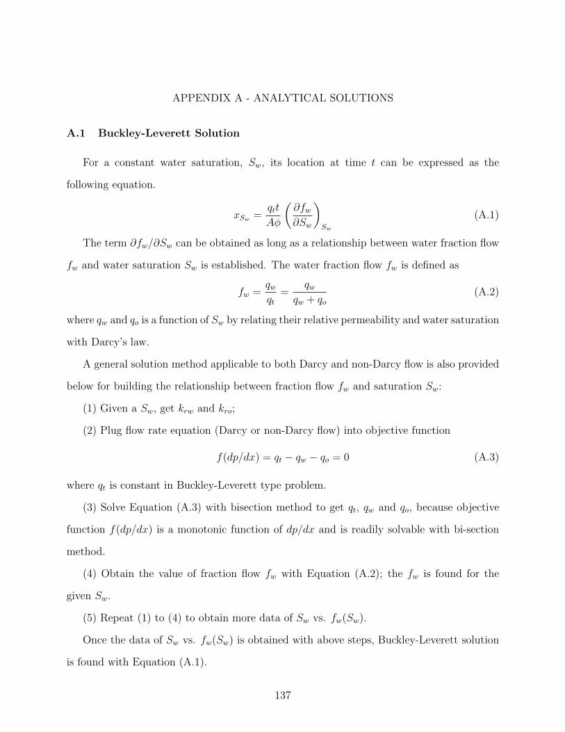
APPENDIX A - ANALYTICAL SOLUTIONS
A.1 Buckley-Leverett Solution
For a constant water saturation, Sw, its location at time t can be expressed as the
following equation.
xSw =qtt
Aφ
(∂fw∂Sw
)Sw
(A.1)
The term ∂fw/∂Sw can be obtained as long as a relationship between water fraction flow
fw and water saturation Sw is established. The water fraction flow fw is defined as
fw =qwqt
=qw
qw + qo(A.2)
where qw and qo is a function of Sw by relating their relative permeability and water saturation
with Darcy’s law.
A general solution method applicable to both Darcy and non-Darcy flow is also provided
below for building the relationship between fraction flow fw and saturation Sw:
(1) Given a Sw, get krw and kro;
(2) Plug flow rate equation (Darcy or non-Darcy flow) into objective function
f(dp/dx) = qt − qw − qo = 0 (A.3)
where qt is constant in Buckley-Leverett type problem.
(3) Solve Equation (A.3) with bisection method to get qt, qw and qo, because objective
function f(dp/dx) is a monotonic function of dp/dx and is readily solvable with bi-section
method.
(4) Obtain the value of fraction flow fw with Equation (A.2); the fw is found for the
given Sw.
(5) Repeat (1) to (4) to obtain more data of Sw vs. fw(Sw).
Once the data of Sw vs. fw(Sw) is obtained with above steps, Buckley-Leverett solution
is found with Equation (A.1).
137

A.2 1-D Consolidation Solution
Jaeger et al. (2007) derives the analytical solution for one-dimensional consolidation
problem. The pore pressure solution during the drainage process shown in Figure 5.9 (c),(d)
and (e) is a function of time t and location z as follows.
p (z, t) = p0
∞∑n=1,3,...
4
nπsin(nπz
2h
)exp
(−n2π2kt
4µSh2
)(A.4)
where p0 is the incremental pressure due to the load on the top of the column shown in
Figure 5.9 (a) and (b) ; p(z, t) is the pressure profile as a function of location and time; h
is total height of the column height; k is the absolute permeability of the column; µ is fluid
viscosity; S is the storage coefficient defined as
S =1
M+
α2
λ+ 2G(A.5)
where M and α are Biot modulus (Jaeger et al., 2007) and Biot coefficient respectively.
The rate of convergence of the series in Equation (A.4) deteriorates as t approaches 0;
Jaeger et al. (2007) also gives an equivalent form Equation (A.4) with more computational
convenience:
p (z, t) = p0
{1−
∞∑n=0
(−1)n[erfc
(2nh+ z
(4kt/µS)0.5
)+ erfc
(2(n+ 1)h− z(4kt/µS)0.5
)]}(A.6)
where erfc(x) is the coerror function defined by
erfc(x) = 1− erf(x) =2√π
∫ ∞x
e−ηdη (A.7)
A.3 2-D Compaction Solution
Abousleiman et al. (1996) derived the analytical solution of the pressure profile in the
2-D compaction problem shown in Figure 5.11. It is assume that the specimen is made
of transversely isotropic poroelastic material, and small strain formulation is adequately
captured the deformation of specimen. The pressure solution is derived as follows based on
above assumptions.
138
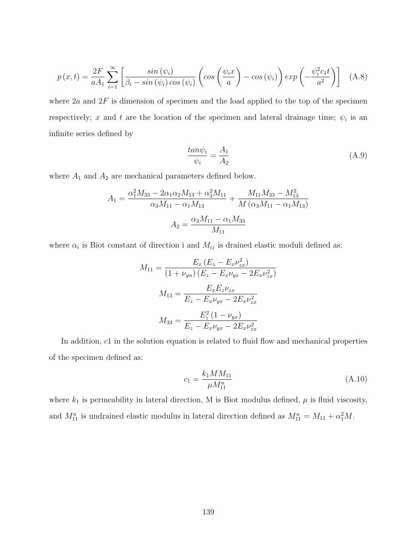
p (x, t) =2F
aA1
∞∑i=1
[sin (ψi)
βi − sin (ψi) cos (ψi)
(cos
(ψix
a
)− cos (ψi)
)exp
(−ψ
2i c1t
a2
)](A.8)
where 2a and 2F is dimension of specimen and the load applied to the top of the specimen
respectively; x and t are the location of the specimen and lateral drainage time; ψi is an
infinite series defined by
tanψiψi
=A1
A2
(A.9)
where A1 and A2 are mechanical parameters defined below.
A1 =α2
1M33 − 2α1α2M13 + α23M11
α3M11 − α1M13
+M11M33 −M2
13
M (α3M11 − α1M13)
A2 =α3M11 − α1M33
M11
where αi is Biot constant of direction i and Mij is drained elastic moduli defined as:
M11 =Ex (Ez − Exν2
zx)
(1 + νyn) (Ez − Exνyx − 2Exν2zx)
M13 =ExEzνzx
Ez − Exνyx − 2Exν2zx
M33 =E2z (1− νyx)
Ez − Exνyx − 2Exν2zx
In addition, c1 in the solution equation is related to fluid flow and mechanical properties
of the specimen defined as:
c1 =k1MM11
µMu11
(A.10)
where k1 is permeability in lateral direction, M is Biot modulus defined, µ is fluid viscosity,
and Mu11 is undrained elastic modulus in lateral direction defined as Mu
11 = M11 + α21M .
139

APPENDIX B - FORMAT OF INPUT AND OUTPUT OF MSFLOW COM
The developed compositional model in this dissertation, MSFLOW COM, is based on
the framework of MSFLOW; thus the general format of input and output follows the user
guide of MSFLOW (Wu, 1998). Accordingly this section only presents the input format for
the parameters not covered by original user guide, such as compositional and geomechanical
properties. Figure B.1 shows a part of snapshot of the input file for MSFLOW COM; the
section ”COMPS” is specifically for compositional input, and geomechanical properties is
inputted in ”ROCKS” section.
B.1 Compositional Data Input - ’COMPS’ Section
The compositional data, mainly including thermodynamic properties of each component
and initial overall composition, z, are input in ”COMPS” section by lines; each line has the
meaning as follows.
• Line 1: Critical temperature of each component in Kelvin
• Line 2: Critical pressure of each component in Pascal
• Line 3: Molar weight of each component
• Line 4: Acentric factor of each component
• Line 5: Critical volume of each component in m3/kgmol
• From line 6 to the third line from last: Binary interaction coefficients
• The last second line: Molecular diffusion coefficients of each component in m2/s; input
0 to ignore molecular diffusion in the simulation.
• Last line: Initial overall composition of each component zi
140
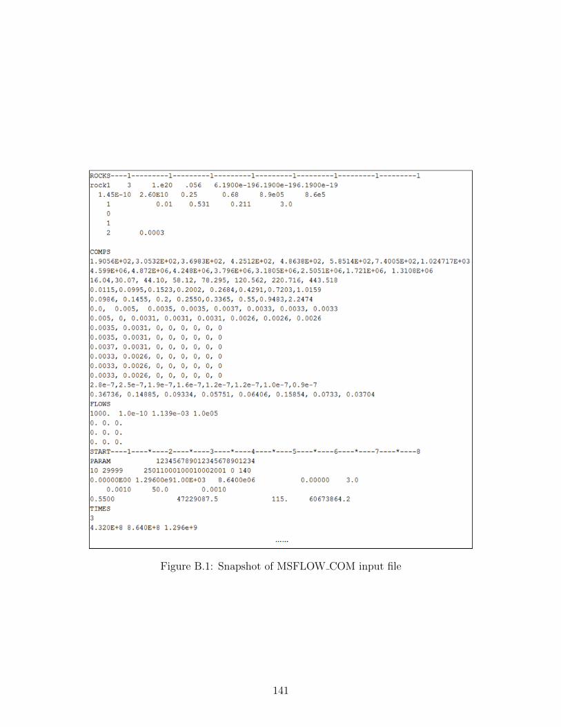
Figure B.1: Snapshot of MSFLOW COM input file
141

B.2 Geomechanical Input - ’ROCKS’ Section
The ’ROCKS’ section follows the original user guide with added inputs of rock geome-
chanical properties and some other parameters in the second line. The parameters in second
line of ’ROCKS’ section from left to right are:
1. Rock compressibility (1/Pa);
2. Young’s modulus (Pa);
3. Poisson’s ratio;
4. Biot’s coefficient;
5. Minimum capillary pressure of oil and gas phase (gas entry pressure) (Pa);
6. Klinkenburg coefficient (Pa).
The last two lines in ’ROCKS’ section are specifically for MSFLOW COM to correlate
porosity and permeability with effective stress respectively. The first integer in the line is the
flag indicating which correlation is used; the other inputs in the line are related calculation
parameters.
B.3 Water Properties and Non-Darcy Coefficients - ’FLOWS’ Section
MSFLOW COM is able to calculate the fluid properties of oil and gas phases through
VLE calculation and related computations for secondary variables. The fluid properties of
water phase are inputted in ’FLOWS’ section. The parameters in first line of ’FLOWS’
section from left to right are:
1. Water density at reference pressure (kg/m3)
2. Water compressibility at reference pressure (1/Pa)
3. Water viscosity at reference pressure (Pa.s)
142

4. Reference pressure (Pa)
The last three lines in ’FLOWS’ section is reserved for the parameters of non-Darcy flow
coefficients, which is not used in this dissertation.
B.4 Other Computation options
The computation options are save in array ’MOP’ in MSFLOW. MSFLOW COM uses
several new MOP flag to set computation options as below.
• MOP(8): if MOP(8) > 0, output composition information of each grid block for each
time step.
• MOP(9): if MOP(9) > 0, only perform VLE calculation and secondary variables ini-
tialization; no simulation. It is usually used to test VLE calculations.
• MOP(10): if MOP(10) > 0, include geomechanical coupling; otherwise, no geomechan-
ical coupling.
For geomechanical coupling simulation, the following parameters should be specified
in one FORTRAN header file of MSFLOW COM source codes:
PARAMETER(MNEQ = MNHC + 2)
PARAMETER(MNK = MNHC +2)
PARAMETER(MXCOM= MNHC + 2)
If there is no geomechanical coupling, above parameters should be changed to MNHC+1.
• MOP(17): if MOP(17) > 0, include the effect of capillary pressure on VLE; otherwise,
no capillarity effect.
B.5 Number of Hydrocarbon Components
The fluid system may vary in the number of hydrocarbon components from reservoir to
reservoir. MSFLOW COM needs to specify the number of hydrocarbon components in one
FORTRAN header file. For example,
143
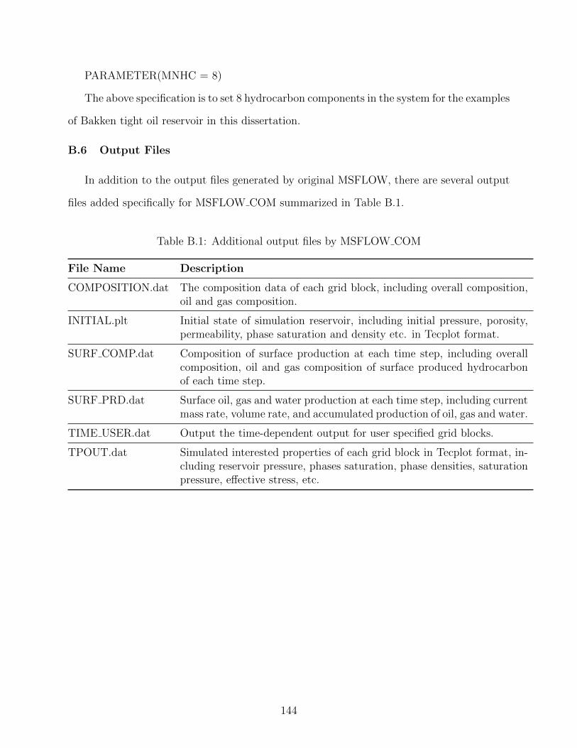
PARAMETER(MNHC = 8)
The above specification is to set 8 hydrocarbon components in the system for the examples
of Bakken tight oil reservoir in this dissertation.
B.6 Output Files
In addition to the output files generated by original MSFLOW, there are several output
files added specifically for MSFLOW COM summarized in Table B.1.
Table B.1: Additional output files by MSFLOW COM
File Name Description
COMPOSITION.dat The composition data of each grid block, including overall composition,oil and gas composition.
INITIAL.plt Initial state of simulation reservoir, including initial pressure, porosity,permeability, phase saturation and density etc. in Tecplot format.
SURF COMP.dat Composition of surface production at each time step, including overallcomposition, oil and gas composition of surface produced hydrocarbonof each time step.
SURF PRD.dat Surface oil, gas and water production at each time step, including currentmass rate, volume rate, and accumulated production of oil, gas and water.
TIME USER.dat Output the time-dependent output for user specified grid blocks.
TPOUT.dat Simulated interested properties of each grid block in Tecplot format, in-cluding reservoir pressure, phases saturation, phase densities, saturationpressure, effective stress, etc.
144