development of a dynamic model for vibration …...i abstract turning operation is a very popular...

Development of A Dynamic Model For

Vibration During Turning Operation And

Numerical Studies

Thesis submitted in accordance with the requirements of the

University of Liverpool for the degree of Doctor in Philosophy

By

Nurhafizzah Hassan

March 2014

To Khairil and Faris

i

Abstract

Turning operation is a very popular process in producing round parts.

Vibration and chatter noise are major issues during turning operation and also

for other machining processes. Some of the effects of vibration and chatter are

short tool life span, tool damage, inaccurate dimension, poor surface finish and

unacceptable noise. The basic dynamic model of turning operation should

include a rotating work piece excited by a force that moves in the longitudinal

direction. Dynamic interaction between a rotating work piece and moving

cutting forces can excite vibration and chatter noise under certain conditions.

This is a very complicated dynamic problem. Vibration and chatter in machining

is one example of moving load problems as the cutter travels along the rotating

work-piece. These moving cutting forces depend on a number of factors and

regenerative chatter is the widely accepted mechanism and model of cutting

forces which then introduce time delays in a dynamic model.

In this investigation, the work piece is modelled as a rotating Rayleigh

beam and the cutting force as a moving load with time delay based on the

regenerative mechanism. The mathematical model developed considers work

piece and cutting tools both as a flexible. Without doubt, this dynamic model of

vibration of work piece in turning operation is more realistic than previous ones

as the dynamic model has multiple-degrees-of-freedom and considers the

vibration of the cutter with regenerative chatter. It is found that the cutting force

model of regenerative chatter which introduces time delay in a dynamic model

leads to interesting dynamic behaviour in the vibration of rotating beams and a

sufficient number of modes must be included to sufficiently represent the

ii

dynamic behaviour. The effects of depth of cut, cutting speed and rotational

speed on the vibration and chatter occurrence are obtained and examined.

Simulated numerical examples are presented. These three different parameters

are vital and definitely influence the dynamic response of deflection in the y and

z directions. The depth of cut is seen to be the most influential on the magnitude

of the deflection. In addition, higher cutting speed combined with high depth of

cut promotes chatter and produces a beating phenomenon whereas rotational

speeds have a moderate influence on the dynamic response. Furthermore,

several turning experiments are conducted that demonstrate vibration and chatter

in the machining operations. There is fairly good qualitative agreement between

the numerical results and the experimental ones.

iii

Acknowledgements

The author is extremely grateful and appreciative to all the contributions

made and advices given that has made this work possible. In particular

acknowledgements are given to the following people and organisations.

First and foremost, to my supervisors, Professor Huajiang Ouyang,

whose encouragement, guidance and invaluable supports from the very

beginning of my PhD study. Without his continuous encouragement and

support, this doctoral thesis would not have been possible. His wide knowledge

and logical way of thinking have been great value for me.

I would also like to thank my second supervisor Prof. Westley

Cantwell, for his encouragement. My thanks also go to Dr Simon James and

Mr Steve Bode for their great help on all the experimental works. Many thanks

as well to Mr. Xiangou Han, Mr. Eric and Professor Minjie Wang for their

valuable helps providing the experimental results. Without that the numerical

results could not be validated properly.

Thanks must also go to my fellow researchers in the Dynamic and

Control Group, including John, Shahrir, Hamid and Yazdi for giving me an

outlet for my frustration.

Special appreciation for my husband, Dr Rd. Khairilhijra and my

beloved son, Rd. Faris Izharkhalish as well as my family especially my

parents who endured this long process with me, for constant support and

unwavering faith throughout my PhD.

iv

And finally, I would like to greatly acknowledge the support by the

Ministry of Education of Malaysia and the University of Tun Hussein Onn

Malaysia (UTHM).

v

Contents

Abstract iii

Acknowledgements v

Contents vii

List of Figures xi

List of Tables xiv

List of Symbols xv

List of Abbreviations xvii

1 INTRODUCTION 1

1.1 Introduction 1

1.2 Motivations 3

1.3 Research aim 5

1.4 Scope of the thesis 7

1.5 Organization of the thesis 9

2 LITERATURES REVIEW AND THEORY 11

2.1 Introduction 12

2.2 Turning operation 12

2.3 Vibration in machining 16

2.4 Chatter noise in machining 17

2.4.1 Mode coupling 21

2.4.2 Regenerative chatter 21

2.5 Regenerative chatter mechanism in tuning operation 23

2.5.1 Chatter modelling theory 26

2.6 Introduction to moving loads problem 31

2.6.1 Moving loads with regenerative chatter in turning

operation 32

2.7 Dynamic model of rotating beam subjected to moving loads 33

vi

2.7.1 Introduction to beam theories 34

2.7.1.1 Euler-Bernouli beam 34

2.7.1.2 Rayleigh beam 35

2.7.1.3 Timoshenko beam 35

2.7.2 Previous dynamic model of a rotating beam/shaft 36

2.8 Factors influencing surface finish of turned metals 42

2.9 Chatter suppression in turning operation 50

2.10 Machining of composite 53

2.11 Factors influencing surface finish of turned composites 55

2.12 Chapter Summary 57

3 DYNAMIC MODEL OF TURNING OPERATION 59

3.1 Introduction 59

3.2 Development of mathematical formulation of Rotating Beam

Subjected to Three Directional Moving Loads with

Regenerative Chatter 60

3.2.1 Boundary Conditions 60

3.2.2 Energy method 63

3.2.3 Lagrange‟s equation 65

3.2.4 Three directional moving cutting forces with

regenerative chatter mechanism 69

3.2.5 Improved dynamic model by adopting Insperger‟s

cutting force model 73

3.2.6 Cutting Tool Equation of Motion 76

3.3 Elastic boundary condition 78

3.4 Methodology for Chatter Analysis / Numerical Integration

methods in vibration analysis 84

3.4.1 Frequency Response Analysis 85

3.4.2 Transient Response Analysis 86

3.4.2.1 Runge-Kutta Method 87

3.4.2.2 Delay Differential Equations 89

3.5 Chapter Summary 91

4 EXPERIMENTAL MODAL ANALYSIS 93

4.1 Introduction 93

4.2 Basic components of experimental modal analysis (EMA) 97

4.2.1 Excitation of structure 98

4.2.2 Mechanism of sensing 100

4.2.3 Data acquisition and processing mechanism 101

4.3 Experimental modal analysis of metal and composite

work piece 101

4.3.1 Free-free boundary 102

4.3.2 Clamped pinned boundary 109

vii

4.4 Experimental modal analysis during machining of cylindrical

metal work piece at DUT 116

4.5 Chapter summary 120

5 NUMERICAL SIMULATION RESULTS 122

5.1 Overview 122

5.2 Parametric studies 123

5.2.1 Clamped pinned (metal work piece) 123

5.2.1.1 Convergence test 123

5.2.1.2 Effect of depth of cut 127

5.2.1.3 Effect of cutting speed 135

5.2.1.4 Effect of rotational speed 140

5.2.2 Elastic boundary (chuck pinned for metal work piece) 144

5.2.2.1 Introduction 144

5.2.2.2 Convergence test 144




5.2.3 Clamped pinned (composite work piece) 166

5.3 Vibration test during turning operation 168

5.4 Chapter summary 173

6 ANALYSIS AND DISCUSSION 175

6.1 Parametric Studies 175

6.1.1 Clamped pinned (metal work piece) 175




6.1.2 Elastic boundary (chuck pinned – metal work piece) 178




6.2 Validation between numerical and experimental results 181

7 CONCLUSIONS AND FUTURE WORKS 183

7.1 Summary of Findings of the Investigation 183

7.2 Contribution to New Knowledge 186

7.3 Recommendations for Further Investigation 187

7.4 List of Publications 188

REFERENCES 189

APPENDIX 201

viii

i. Appendix A1 - Calculation of deflection, v and w for

clamp-pinned boundary 207

ii. Appendix A2 - Derivation of Delay Differential equation for


iii. Appendix A3 - Time delay function 211

iv. Appendix A4 - Determination of mode shape function for


v. Appendix A5 - First derivation of mode shape function for


vi. Appendix A6 - Second derivation of mode shape function for

clamp pinned boundary 214

vii. Appendix A7 - Calculation of cutting speed 215

viii. Appendix A8 - Calculation of deflection, v and w for elastic

Boundary 216

ix. Appendix A9 - Derivation of Delay Differential equation for

elastic boundary 219

x. Appendix A10 - Determination of mode shape function for


xi. Appendix A11 - First derivation of mode shape function for


xii. Appendix A12 - Second derivation of mode shape function for


xiii. Appendix A13 - Calculation of C1, C2, C3 and C4 variables 225

ix

List of Figures

2.1 Conventional lathe machine at University of Liverpool........................ 13

2.2 Schematic illustration of a turning operation ........................................ 15

2.3 (a) Chatter mark ................................................................................... 18

2.3 (b) Chatter mark on turned work piece.................................................. 18

2.4 (a) Segmented chips .............................................................................. 19

2.4 (b) Discontinuous chips ......................................................................... 19

2.5 Regenerative chatter mechanism ........................................................... 24

2.6 Rotating shaft subjected to a moving load with three

perpendicular forces .............................................................................. 33

2.7 Torque and bending moment generated from Px and Pz force

components translated to the neutral axis ...............................................33

2.8 Elements of surface machine surface texture ........................................ 43

3.1 Comparison between current dynamic model coordinate system

and Insperger‟s coordinate system (a) current dynamic model

coordinate system (b) Insperger‟s coordinate system …………....…... 74

3.2 Example of one value of 𝛽𝑛 showing the beam classical mode

Shape ......................................................................................................81

3.3 Graph of new fitted theoretical (marked by red) and measured

(marked by blue) mode shapes for the chuck-tailstock ......................... 84

4.1 Route to vibration analysis .................................................................... 95

4.2 General layout of EMA ..........................................................................98

4.3 Impact Hammer ....................................................................................100

4.4 Accelerometer ...................................................................................... 101

4.5 Experimental set up for the cylindrical metal work piece of

x

free-free boundary …………………………....................................... 102

4.6 Apparatus used for modal testing (a) PCB impact hammer

(b) Kistler accelerometer (c) 12 channels LMS system .......................103

4.7 A cylindrical metal work piece with its five measured locations ........103

4.8 The experimental mode shapes of the cylindrical metal work

piece for free-free boundary..................................................................106

4.9 The experimental mode shapes of the cylindrical composite work

piece for free-free boundary ……………………………………….…108

4.10 Modal test setup for cylindrical work piece in clamped-pinned

boundary condition …………………………………………….……..109

4.11 Kistler accelerometer and Micro-epsilon laser sensor ………….…….110

4.12 The experimental mode shapes of the cylindrical metal work

piece for clamp-pinned boundary …………….................................…112

4.13 Responses from laser sensor showing the noise ……………………...113

4.14 Modal test setup for clamped-pinned boundary in y and z

direction ................................................................................................115

4.15 Schematic illustration of the vibration test set-up ……………………117

4.16 Two views of the experimental rig ………………………………...... 118

5.1 Dynamic response of deflection, v (y direction) with (a) one mode

(b) two modes (c) three modes (d) four modes (e) five modes. Note

that the unit for x axis is time, t (s) and y axis is the dynamic

response, m........................................................................................... 125

5.2 Dynamic response of deflection, w (z direction) with (a) one mode



response, m........................................................................................... 126

5.3 Dynamic response of deflection, v at different depths of cut with

one mode (cutting speed = 0.2228 m/s, the rotational speed

= 1250 rev/min and the feed rate = 0.3 mm/rev).................................. 128

5.4 Dynamic response of deflection, w at different depths of cut with

one mode (cutting speed = 0.2228 m/s, the rotational speed

= 1250 rev/min and the feed rate = 0.3 mm/rev) ................................. 129


two modes (cutting speed = 0.2228 m/s, the rotational speed =

xi

1250 rev/min and the feed rate = 0.3 mm/rev) .................................... 130


two modes (cutting speed = 0.2228 m/s, the rotational speed =


5.7 Phenomenon of beats ............................................................................133


three modes (cutting speed = 0.2228 m/s, the rotational speed =



three modes (cutting speed = 0.2228 m/s, the rotational speed =

1250 rev/min and the feed rate = 0.3 mm/rev)..................................... 134


four modes (cutting speed = 0.2228 m/s, the rotational speed =

1250 rev/min and the feed rate = 0.3 mm/rev)..................................... 135


four modes (cutting speed = 0.2228 m/s, the rotational speed =


5.12 Dynamic response of deflection, v at different cutting speeds with

one mode (depth of cut = 3.00 mm, rotational speed = 1250 rev/min

and the feed rate = 0.3 mm/rev) ........................................................... 137

5.13 Dynamic response of deflection, w at different cutting speeds with




two modes (depth of cut = 3.00 mm, rotational speed = 1250 rev/min






three modes (depth of cut = 3.00 mm, rotational speed = 1250

rev/min and the feed rate = 0.3 mm/rev) ............................................. 140



xii



four modes (depth of cut = 3.00 mm, rotational speed = 1250





5.20 Dynamic response of deflection, v at different rotational speeds

with one mode (depth of cut = 3.00 mm, cutting speed = 0.2228

m/s and the feed rate = 0.3 mm/rev) .................................................... 143

5.21 Dynamic response of deflection, w at different rotational speeds

with one mode (depth of cut = 3 mm, cutting speed = 0.2228 m/s


5.22 Dynamic response of deflection, v at different rotational speeds

with two modes (depth of cut = 3.00 mm, cutting speed = 0.2228


5.23 Dynamic response of deflection, w at different rotational speeds

with two modes (depth of cut = 3.00 mm, cutting speed = 0.2228


5.24 Dynamic response of deflection, v (y direction) with (a) one mode



response, m .......................................................................................... 149

5.25 Dynamic response of deflection, w (z direction) with (a) one mode



response, m .......................................................................................... 150


one mode (1250 rev/min, cutting speed = 2.228m/s and feed rate is

0.3 mm/rev) ......................................................................................... 152


one mode (1250 rev/min, cutting speed = 2.228m/s and feed rate is

0.3 mm/rev) ......................................................................................... 153


xiii

two modes (1250 rev/min, cutting speed = 2.228m/s and feed rate

is 0.3 mm/rev) .................................................................................... 154


two modes (1250 rev/min, cutting speed = 2.228m/s and feed

rate is 0.3 mm/rev) ..............................................................................155


three modes (1250 rev/min, cutting speed = 2.228m/s and feed rate

is 0.3 mm/rev) .................................................................................... 156


three modes (1250 rev/min, cutting speed = 2.228m/s and feed rate

is 0.3 mm/rev) .................................................................................... 157


four modes (1250 rev/min, cutting speed = 2.228m/s and feed rate

is 0.3 mm/rev) .................................................................................... 158


four modes (1250 rev/min, cutting speed = 2.228m/s and feed rate

is 0.3 mm/rev) .................................................................................... 159

5.34 Dynamic response of deflection, v at different cutting speed with


and feed rate is 0.3 mm/rev) .............................................................. 160

5.35 Dynamic response of deflection, w at different cutting speed with











rev/min and feed rate is 0.3 mm/rev) ................................................ 163



xiv








5.42 Dynamic response of deflection, v at different rotational speed

with one mode (depth of cut = 3.00 mm, cutting speed = 2.228 m/s

and feed rate = 0.3 mm/rev) .............................................................. 165

5.43 Dynamic response of deflection, w at different rotational speed

with one mode (depth of cut = 3.00 mm, cutting speed = 2.228 m/s



with two modes (depth of cut = 3.00 mm, cutting speed = 2.228 m/s



with two modes (depth of cut = 3.00 mm, cutting speed = 2.228 m/s



with three modes (depth of cut = 3.00 mm, cutting speed = 2.228 m/s



with three modes (depth of cut = 3.00 mm, cutting speed = 2.228 m/s



with four modes (depth of cut = 3.00 mm, cutting speed = 2.228 m/s



with four modes (depth of cut = 3.00 mm, cutting speed = 2.228 m/s


5.50 Dynamic response of deflection, w at one mode (depth of cut =

0.25 mm, cutting speed = 0.2228 m/s, rotational speed = 1250

rev/min and feed rate = 0.3 mm/rev) ................................................. 174

xv

5.51 Dynamic response of deflection, w at one mode (depth of cut =

0.25 mm, cutting speed = 0.2228 m/s, rotational speed = 1250

rev/min and feed rate = 0.3 mm/rev) ................................................... 174

5.52 Dynamic response of deflection, v at one mode (depth of cut

= 3.0 mm, cutting speed = 0.2228 m/s, rotational speed =

1250 rev/min and feed rate = 0.3 mm/rev) .......................................... 175

5.53 Dynamic response of deflection, w at one mode (depth of cut

= 3.0 mm, cutting speed = 0.2228 m/s, rotational speed =

1250 rev/min and feed rate = 0.3 mm/rev) .......................................... 175

5.54 The being machined work piece of experiment 1 ……………........... 177

5.55 Deflections in time domain of experiment 1 ……………………….. 177

5.56 The being machined work piece of experiment 2 shown chatter

occurrence ………………………………………………….....……... 178

5.57 Deflections in time domain of experiment 2 …………………….….. 179

xvi

List of Tables

2.1 Factors affecting surface roughness and their major investigators ....... 47

2.2 Factors affecting surface roughness and major investigators ............... 56

3.1 Possible boundary conditions ................................................................ 61

3.2 Matching table for both coordinate systems ..........................................74

3.3 Tabulated measured mode shapes, frequencies and 𝛽𝑛 ......................... 80

3.4 Example calculation for fitting the mode shape of 2Z .......................... 83

3.5 A technique of solving DDEs by reducing them to a sequence

of ODEs ................................................................................................ 90

4.1 Nominal material properties of cylindrical metal work piece ..............104

4.2 The three measured natural frequencies of the cylindical metal

work piece .............................................................................................104

4.3 Nominal material properties of cylindrical composite work piece ......106

4.4 The three measured natural frequencies of the cylindrical composite

work piece ………………………………………………………….…107

4.5 The five measured clamped-pinned natural frequencies of the

cylindrical metal work-piece ………………………………………....110

4.6 Properties of the cylindrical metal work piece used in the DUT test ...114

4.7 Free-free boundary condition for cylindrical metal work piece ……...114

4.8 Clamped-pinned boundary condition for metal work piece

(y direction) ……………………………………………………….…..115

4.9 Clamped-pinned boundary condition for metal work piece

(z direction) …………………………………………………….……..116

4.10 Cutting conditions and work piece characteristics ………………...... 118

5.1 Cutting parameters and work piece characteristics used during

xvii

turning operation …………………………………………….…....... 176

6.1 Comparison between theoretical and experimental of dynamic

responses at both v and w..................................................................... 189

xviii

List of Symbols

A Cross-sectional area (mm2)

Bl(t) A time varying matrix

cy Damping

d Work piece diameter in mm

E Young‟s Modulus (kg/m3)

f Feed rate (m/rev)

f (t) Driving force

f. f. S Speed of the feed

F(s) Laplace‟s Transform

Ff Feed cutting force (N)

Ff (t) A time varying dynamic force due to cutting process

h Instantaneous depth of cut (mm)

h(t) Instantaneous chip thickness

ho Intended cut (mm)

I Moment of inertia (kgm2)

ky Stiffness of the cutting tool

Kx Cutting force coefficient (unitless)

Ky Cutting force coefficient (unitless)

Kz Cutting force coefficient (unitless)

l Length (mm) my Mass

Mz Bending moment

N Spindle speed in rev/min

Px Feed force

xix

Py Tangential force

Py(t) The magnitude of tangential cutting force

Pz Radial force

𝑞 𝑗 A generalized velocity

Q A generalize cutting force component

𝑄𝑗(𝑛)

A non-conservative generalized force

s(t) Variable length from the spindle end to the location of the cutter

s2X(s) Laplace‟s Transform of acceleration

t Time (s)

T Kinetic energy (J)

T Torque

v Deflection in z direction (mm)

V Strain energy of the beam

V Cutting speed in m/min or ft/min

w Deflection in y direction (mm)

w Depth of cut in mm

W(x) A normal mode or characteristic function of the beam

y Displacement

y(t - ) Outside surface

y(t) Inside surface

Z Measured mode shape

αi(t) Corresponding modal coordinate

βi(t) Corresponding modal coordinate

δ Logarithmic decrement

ρ Mass density (GPa)

σ Root mean square

τ Time delay (s)

Shear plane angle

ω Angular rotation (rad/s)

n Theoretical frequency (Hz)

i(x) A spatial function that satisfies the boundary condition of the beam

Ω Rotary speed (rev/min)

xx

List of Abbreviations

1D One-dimensional

3D Three-dimensional

DD Dimensional deviations

DDEs Delay differential equations

DOF Degree of freedom

DUT Dalian University of Technology

EMA Experimental modal analysis

FFT Fast Fourier Transform

FRFs Frequency response functions

FRP Fibre reinforced polymer

GFRP Glass fibre reinforced polymer

IRFs Impulse response functions

MDOF Multiple degree of freedoms

ODEs Ordinary differential equations

SDOF Single degree of freedom

TDOF Two degrees of freedom

1

Chapter 1

Introduction

1.1 Introduction

This chapter contains a general introduction of the research (Section 1.1),

motivations for the work (Section 1.2), research aim (Section 1.3) and scope of

the thesis (Section 1.4). Section 1.5 describes the organisation of the thesis.

There are many different ways in which a product can be manufactured.

Conventional techniques encompass processes such as machining, metal

forming, injection moulding, die casting, stamping and many others. Machining

is one of the basic and most widely used operations necessary to cut things to

size and to finish off edges, dimensions and other aspect of a finished assembly

part. Machining is a term that covers a large collection of manufacturing

processes designed to remove unwanted material, usually in the form of chips,

from a work piece. Machining is also used to convert basic geometrical shapes

or shapes manufactured using different technologies (castings, forgings) into

desired shapes, with size and finish specified to fulfil design requirements. A

blank work piece is converted into a final product by cutting extra material away

by turning, milling, drilling, boring or grinding operation. Generally, it can be

said that most of manufactured product has components that require machining.

2

Therefore, this collection of processes is one of the most important among the

basic manufacturing processes because of the value added to the final product.

In general, work pieces used in machining are made of metals due to

their popular physical and mechanical properties in most engineering

applications. In automotive industry for example, most of the parts are made

from metals and their alloys. In cars, steel can crumple to absorb different

impacts and hence are used to create the underlying chassis or cage beneath the

body that forms the skeleton of the vehicle, door beams, roofs, and other parts.

A large number of manufacturers these days are gradually trying to substitute

metals due to their shortcomings such as weight, and corrosion (for some

metals) if not painted or coated. Plastic materials especially composites become

prominent to avoid these drawbacks.

Over the years, manufacturers begin to explore other materials that cost

less and perform better, being lighter, for instance or more corrosion resistant.

Metals have been steadily incorporated with composite materials as they offer

special advantages mentioned earlier. Although composite parts may be

produced by other fabrication techniques like near net shape forming and

modified casting, they still require further subsequent machining to facilitate

precise dimensions to the part. Composites, unlike metals, are not isotropic and

consist of both unique resins and fibres. Therefore machining composites in any

post processing operation to get to the final part is indeed different.

Machining of composite has become an exciting subject in recent years

since the use of composite materials has increased tremendously in various areas

in science and technology. With regard to the increase use of composites in

many industries such as aerospace sector, the need to machine composite

materials adequately has increased enormously. Typically composites are

layered construction unite a resin matrix with normally discrete layers of brittle

fibre reinforcement. In comparison to metals, composite react very differently

and not so predictably during machining. The tool encounters continuously

alternate fibres and matrix, which response differently. In composite, the

material behaviour is not only inhomogeneous, but also depends on diverse fibre

3

and matrix properties, fibre orientation at the point of contact, and the relative

volumes of fibre and matrix (Basavarajappa et al., 2006)

1.2 Motivations

One of the most-known machining processes is turning. Turning

operation is one of the oldest and most versatile conventional ways to produce

round parts by means of a single point cutting tool. Typical products made

include parts as small as miniature screws for eyeglass frame hinges and as large

as rolls for rolling mills, cylinders, gun barrels and turbine shafts for

hydroelectric power plants. Normally turning is performed on a lathe machine

where one end of the work piece is fixed to the spindle and the other end pin

mounted to the tails stock. The tool is fed either linearly in the direction parallel

or perpendicular to the axis of rotation of the work piece. The work piece will

experience a rotary motion whereas the cutting tool will experience a linear

translation.

Work piece and cutting tool come in contact with each other during

turning operation. This dynamic interaction between a rotating work piece and

moving cutting forces will suppress vibration and occasionally under certain

conditions it will excite chatter noise. The growing vibrations increase the

cutting forces and may chip the tool and produce a poor surface finish. Harder

regulations in terms of the noise levels also affected the operator environment.

This is a very complicated dynamic problem. Vibration and chatter noise are

major issues not just for turning operation but for any other machining

processes. Short tool life span, tool damage, inaccurate dimension, poor surface

finish are some distinctive adverse effects of vibration during machining. In

addition, noise is a nuisance and unacceptable noise to the well-being of the

operator. Manufactured products or components should have a good surface

finish for better quality, reliability, excellent performance and meet customer

requirements. In most cases poor surface finish contributes to irregularities in

the surface and may form nucleation sites of cracks or corrosion.

4

There are two groups of researchers who study on vibration and chatter

noise in turning operation which are the structural dynamicists and manufacture

engineers. The structural dynamicists studied on vibration of a shaft spinning

about its longitudinal axis subjected to moving load (Ouyang, 2011). Vibration

and chatter noise in turning operation is one example of the moving load

problems as the cutter travels along the rotating work piece and this generate

three directional moving cutting forces. The rotating work piece (usually treated

as a beam or shaft) can be modelled in more than one beam theory. In general

there are four beam theories used which are Euler-Bernoulli, Rayleigh, shear

and Timoshenko. The more sophisticated beam theories employed into the

dynamic model of the turned work piece, the more accurate is the model. On the

other hand, it is time consuming during computational work since sophisticated

theories consider numerous interactions between several known variables. From

the established dynamic model, vibration of the work piece during turning

operation can be simulated.

The second group is from manufacturing engineers. Most of the

manufacture engineers use simplified dynamic models for the work piece and do

not treat it as well as structural dynamicists. The cutting tools often modelled as

a lumped mass having one or two degrees of freedom (for describing motions of

the cutting tool in the main cutting force direction). On the other hand, the

manufacture engineer‟s cutting forces models are more realistic as they usually

model the cutting tool as a single degree of freedom (SDOF) or two degree of

freedom (TDOF) with regenerative chatter mechanism. Mode coupling and

regeneration of chatter are two common chatter mechanisms occur during

machining. Moving cutting forces in turning operation depend on a number of

factors and regenerative chatter is the widely accepted mechanism which then

introduces time delays in the established dynamic model. The length of this

delay in turning operation is the time period for one revolution of the work

piece.

A substantial amount of research on dynamic model of vibration for

turned metal had been investigated over the years but unfortunately there has

been less research on this area especially in turning of composites. The dynamic

5

models developed in this study assumed a straightforward and common

behaviour which captures some basic features of a turning operation in

machining, in which a cutting tool is moved in the axial direction against a work

piece that is rotating rapidly. This dynamic model should work well for both of

the work piece, metal and composite. In the past, most studies of dynamic model

of turning operation have generally assumed the work piece to be rigid and have,

therefore, ignored work piece deformation. However, in practice, the work piece

undergoes deformation as a result of an external force by the cutting tool. This

deformation affects and changes the chip thickness. In this thesis, the main

contribution is to combine both dynamic models concept from those two groups;

structural dynamicists and manufacturing engineers and develop a new

mathematical model considering the work piece and cutting tools as a flexible

work piece and flexible cutting tools. In addition the effect of the deflection-

dependence of the moving cutting forces with regenerative chatter on the

dynamic behaviour of the system at various travelling cutting speeds is also

investigated.

1.3 Research Aim

The reliability of the developed dynamic model of turning operation is

required to be simulated first for metal work piece. This has to be done right

before considering simulating the composite material into the established

dynamic model. There are two boundary conditions simulated in the developed

dynamics model for metal work piece; clamp pinned and elastic boundary

(chuck-tail stock) boundary. Each boundary condition was simulated to

determine the work piece natural frequency and mode shapes. The results from

the simulation are needed to be validated with the experimental results to realize

the reliability of the dynamics model. In the beginning, the dynamic responses

are set to be measured by laser sensor but unfortunately the laser is not sensitive

enough. From the initial results, it is found that they had big differences

compared to the numerical results (The details of the result were discussed in

Chapter 4). Due to lack of the equipment in measuring the deflection of the

6

work piece and the moving cutting forces, the produced data could not be used.

Instead, a collaboration data from a collaborator in China had to be used.

However, there has not been a reduced quality of the research. In addition, the

dynamic model developed is originally aimed to be used for work pieces made

from composite materials but since enough original work on metal work pieces

has been done, the thesis is focused on metals. Composites are studied only

during the preliminary stage of this research. Previous works on composites and

their characteristics are also discussed in the literature review in the context of

vibration and chatter noise during turning of composite as they can be useful in

future.

Due to several encountered problems mentioned earlier, the focus of the

research had to be changed slightly to the development of mathematical aspect

of coding and numerical simulation after consultation with the supervisor. Thus,

the main aim of this study is to develop a dynamic model for turning metal work

pieces which considers flexible work piece and flexible cutting tool with the

regenerative chatter effects. This can be achieved by pursuing several tasks: (1)

to understand what affect the vibration and chatter noise during turning in a

quantitative manner and then find ways of alleviating this problem by

parametric studies, (2) to develop the mathematical model which is then will be

validated against experimental results from a collaborator from China due to

lack of equipment and technical support within the student‟s own school. The

validated model will be used to simulate structural modifications in order to

identify means of design improvements and vibration reduction. The developed

models permit a full analysis and discussion of the interaction between the work

piece and the tool.

7

1.4 Scope of the thesis

The scope of the research covers several key areas which are given as

follows:

i. Identify the main factors that influence vibration and chatter noise

of turned metal and composite work pieces

One step towards a solution to the vibration and chatter noise problems is

to investigate what kind of vibration that is present during turning

operation. Thus, it is vital to investigate and identify several factors that

will influence this vibration and chatter noise of turned metals and

composites.

ii. Literatures review on dynamic model of turned metal with

regenerative chatter

The next scope is to provide a brief but comprehensive survey on the

currently available dynamic models of turned metal and composite.

iii. Develop a dynamic model for the vibration of rotating Rayleigh

beam subjected to three directional moving cutting forces with

regenerative chatter and flexible cutting tool and code it in

MATLAB software

Develop a mathematical model for the behaviour of turning operation

and validate the realistic dynamic model through experiments. The work

piece is modelled as a rotating shaft (Rayleigh beam) subjected to a three

directional moving cutting forces with regenerative chatter. The dynamic

response of a rotating shaft is based on two boundary conditions which

are the clamped pinned and elastic boundaries. This dynamic model of

vibration of work piece in turning operation is more realistic as the

dynamic model has multiple degrees of freedom and considers the

8

vibration of the cutter with regenerative chatter mechanism. It will

involve great effort since the dynamic model for turning is very

complicated in mathematics. Simulation is then needed to imitate the

dynamic behaviour of the turning process subjected to moving cutting

forces with regenerative chatter mechanism prior to actual machining

and numerical examples are analysed accordingly.

iv. Numerical simulation of reducing vibration by parametric studies of

machining parameters

One has to predict and visualize the effect of several cutting and machine

parameters to the turned metal parts so that a good finished product can

be achieved. It is known that several machining parameters such as

cutting speed, depth of cut, feed rate and rotational speed affect the

surface finish of turned work piece. By means of the dynamic model

established above, these machining parameters and work piece

characteristics are simulated to observe how they influence surface finish

and vibration of turned work piece. The effects of depth of cut, the

rotational speed and cutting speed of the cutter on the vibration and

chatter occurrence are examined. Unfortunately due to the lack of

equipment, most of the work is done in the form of numerical simulation

and the validation of the developed dynamic model is made by using and

comparing the data from the collaborate group in China. Only modal

testing of metal and composite work pieces has been conducted. Ideally,

experiments will be performed to test the machinability of metal

according to the recommended cutting and machining parameters and

validate the established dynamic model.

9

1.5 Organization of the thesis

The thesis consists of seven chapters describing all the works done in the

research. These chapters are structured as follows:

Chapter 1 described the introduction and background of the research.

The motivation behind the research was also stressed out in this chapter. In

addition, the aim of the research was also laid out. The scopes of the research as

well were also highlighted as a framework of the research.

Chapter 2 presents a brief literature review on the background of metal

cutting especially turning operation and machining of composite. The influence

factors contributing to the surface finish of the turned metals and composites

were also explained. The introduction to vibration and chatter noise in

machining and what would contribute to the occurrence of chatter noise in

turning of metals or composites are also presented. Two different mechanisms of

chatter noise usually occurred in machining process were also discussed. The

basic vibration/chatter theory of 1-2 degree of freedom (DOF) used by most

manufacturing people is discussed. The classical beam theories used in this

research were also explained. Lastly, the methods to suppress vibration and

chatter noise in turning operation by means of active and passive controlled

were also reviewed in this chapter.

Chapter 3 presents the theory and development details of dynamic model

employed in turning operation. The classical beam theories used in this research

were also explained. A number of regenerative chatter models developed were

also presented. This chapter also introduces the dynamic models of a rotating

shaft subjected to three directional moving cutting forces with regenerative

chatter mechanism. The sequence of improved mathematical formulation

developed was also presented and discussed.

Chapter 4 explains the experimental modal analysis and discuss several

experiments done to determine the natural frequency and mode shapes for the

10

work piece. Some cutting tests were also carried out on metals to identify the

cutting force coefficient and cutting parameter effects.

Chapter 5 describes the numerical simulation works done and discuss the

outcomes of the simulation which includes the parametric studies done to

evaluate the effect of different cutting parameters on vibration.

Chapter 6 explained the detail analysis and discussion on the results from

the parametric studies. Explanation on how the dynamic model developed is

validated is also stated.

Chapter 7 concludes the research on numerical studies of vibration in

turning operation. In addition, the contribution of the research are summarised

and future research directions are proposed. Published journal and conference

proceeding papers are also listed.

11

Chapter 2

Literatures Review and Theory

The organisation of this literature review is as follows; Section 2.2

presents the fundamental knowledge of turning operation cutting parameters

such as cutting speed, depth of cut and feed rate. Section 2.3 describes the

vibration in turning operation and Section 2.4 explains the phenomena of chatter

noise in turning operation. Two different chatter mechanisms are described and

discussed. Section 2.5 discusses the mechanism of regenerative chatter and some

of the equations involved. In the meantime, Section 2.6 introduces some

fundamental concepts of moving load dynamics problem. A number of dynamic

responses of a rotating shaft subjected to moving load are reviewed in Section

2.7 with references for readers to explore at their own time. Several factors that

influence the vibration and surface finish of turned metal are discussed in

section 2.8. In Section 2.9, machining of composite will be discussed briefly and

some factors contributing to the vibration and surface finish of turned

composites is explained in Section 10. Last but not least in section 2.11, various

chatter suppression methods in turning operation are discussed. Lastly, section

2.12 draws conclusions and presents an outlook of this research.

12

2.1 Introduction

Most machining today is carried out to shape metals and alloys. Many

composites and plastic products are also machined. As regards to size,

components from watch parts to aircraft wing parts are machined. In the

engineering industry, the term machining is used to cover chip forming

operations. Machining is an operation in which a thin layer of metal is removed

by a wedge shaped tool from a larger body (Trent and Wright, 2000). It includes

various processes in which a piece of raw material is cut into a desired final

shape and size by a controlled material removal process. Machining also is one

of the most widely used methods of producing the final shape of the

manufactured products.

2.2 Turning Operation

There are three principals of machining process which are turning,

drilling and milling. Other operations fall into miscellaneous categories such as

shaping, planning, boring, broaching and sawing. The focus of this thesis is on

turning operation. Turning operation is one of the oldest and most versatile

conventional ways of producing parts that are basically in round shape. Turning

means that the work piece is rotating while it is being machined. The starting

material is usually a work piece that has been made by other processes such as

casting, forging or extrusion.

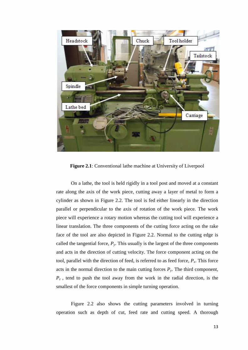
A conventional lathe which normally turning is performed is illustrated

in Figure 2.1. One end of the work piece is fixed to the spindle by chuck and the

other end is pin mounted to the tails stock as can be seen in Figure 2.1. The

machine consists of a headstock which is mounted on the lathe bed. The

headstock contains the spindle that rotates the cylindrical work piece that is held

in the chuck. The single point cutting tool is placed at the tool holder that is

mounted on the cross slide. The cross slide is in turn mounted on the carriage.

13

Figure 2.1: Conventional lathe machine at University of Liverpool

On a lathe, the tool is held rigidly in a tool post and moved at a constant

rate along the axis of the work piece, cutting away a layer of metal to form a

cylinder as shown in Figure 2.2. The tool is fed either linearly in the direction

parallel or perpendicular to the axis of rotation of the work piece. The work

piece will experience a rotary motion whereas the cutting tool will experience a

linear translation. The three components of the cutting force acting on the rake

face of the tool are also depicted in Figure 2.2. Normal to the cutting edge is

called the tangential force, Py. This usually is the largest of the three components

and acts in the direction of cutting velocity. The force component acting on the

tool, parallel with the direction of feed, is referred to as feed force, Px. This force

acts in the normal direction to the main cutting forces Py. The third component,

Pz , tend to push the tool away from the work in the radial direction, is the

smallest of the force components in simple turning operation.

Figure 2.2 also shows the cutting parameters involved in turning

operation such as depth of cut, feed rate and cutting speed. A thorough

14

knowledge of the variable factors of cutting speeds, feed rate and depth of cut

must be understood (Trent and Wright, 2000) and below are the definitions for

each of the turning process parameters.

The cutting speed (V) is the rate at which the uncut surface of the work

passes the cutting edge of the tool, usually expressed in units of m/min or ft/min.

The cutting speed of a tool is the speed at which the metal is removed by the

tool from the work piece. Cutting speed is usually between 3 and 200 m/min (10

and 600 ft/min) (Trent and Wright, 2000). The cutting speed can be calculated

using the equation 2.1 below:

𝑉 =𝑁 𝑑

1000 (2.1)

where V is the cutting speed (m/min), N is the spindle speed (rev/min)

and d is the work piece diameter. Since 𝜋𝑑 is constant, thus the cutting speed

depends on the spindle speed in which it is usually being determined first before

actual turning operation according to Trent and Wright (2000).

The feed rate (f) is the distance moved by the tool in an axial direction at

each revolution of the work piece. The feed rate may be as low as 0.0125 mm

(0.0005 in) per revolution and with very heavy cutting, it can go up to 2.5 mm

(0.1 in) per revolution as mentioned by Trent and Wright (2000). Equation 2.2 is

normally used to calculate the feed rate;

𝐹𝑒𝑒𝑑 𝑅𝑎𝑡𝑒 = 𝑓𝑒𝑒𝑑 x 𝑁 (2.2)

where N is the spindle speed (rev/min), feed is in mm/rev and the unit of feed

rate is in mm/min.

The depth of cut (w) is the thickness of the metal removed from the work

piece, measured in radial direction. A depth of cut is the perpendicular distance

measured from the machined surface to the uncut surface of the work piece. A

15

depth of cut may vary from zero to over 25 mm (1 in). Equation 2.3 is

sometimes used to define a depth of cut;

𝐷𝑒𝑝𝑡ℎ 𝑜𝑓 𝑐𝑢𝑡 =𝑑1−𝑑2

2 (2.3)

where 𝑑1 is diameter of the work surface before cutting and 𝑑2 is the diameter

of the machined surface. The unit of a depth of cut is in mm.

The rotational speed () or sometimes called speed of revolution is the

number of complete rotations, revolutions, cycles, or turns per time unit. It is a

cyclic frequency, measured in radians per second or in hertz or in revolutions

per minute (rev/min or min-1

) or revolutions per second in everyday life.

Equation 2.4 is used to define a rotational speed;

𝜔 = 𝑣

𝑟 (2.4)

where v is a tangential speed and r is a radial distance.

Figure 2.2: Schematic illustration of a turning operation

http://en.wikipedia.org/wiki/Frequency

http://en.wikipedia.org/wiki/Radians_per_second

http://en.wikipedia.org/wiki/Hertz

http://en.wikipedia.org/wiki/Revolutions_per_minute



http://en.wikipedia.org/wiki/Revolutions_per_second

http://en.wikipedia.org/wiki/Speed#Tangential_speed

16

2.3 Vibration in Machining

Vibrations in machining are complex phenomena. During machining,

work pieces are being cut and remove in discrete chunks. Each time the cutting

tool takes a bite, it exerts a force on the work piece that was not there an instant

ago. The work piece responds to this force by deflecting or by molecules

compressing closer together, and generate mechanical stress. This mechanical

stress travels through the work piece as a whole and the work piece acts like a

spring to deflect and then return into shape. This explains vibration phenomenon

during machining process.

Vibration is defined as any motion that repeats itself after interval of

time and can be classified in several ways (Rao, 1995). There are two type of

vibrations occurred during machining; forced and self-excited vibration. Forced

vibration is generally caused by some periodic applied force present in the

machine tool, such as that from gear drives, imbalance of the machine tool

components, misalignment, and motors and pumps (Altintas, 2000). The basic

solution to forced vibration is to isolate or remove the forcing element. If the

forcing frequency is at or near the natural frequency of a component of a

machine tool system, one of the frequencies may be raised or lowered. The

amplitude of vibration can be reduced by increasing the stiffness or by

employing a damping system.

The force acting on a vibrating system is usually external to the system

and independent of the motion. However, there are systems for which the

exciting force is a function of the motion parameters of the system, such as

displacement, velocity or acceleration. Such systems are called self-excited

vibrating systems, since the motion itself produces the exciting force (Rao,

1995). In machining, self excited vibration comes from the dynamic interaction

of dynamics of chip removal process and structural dynamics of machine tool.

Chatter is one of the examples of self excited vibrations that feeds on itself as

the cutting tool moves across the work piece and generate distinctive loud and

17

unwanted noise. This unwanted noise is known in machining world as chatter

noise.

2.4 Chatter Noise in Turning Operation

Chatter noise in machining is complex phenomena too similar to the

vibration in machining. Chatter is an abnormal tool behaviour which it is one of

the most critical problems in machining process and must be avoided to improve

the dimensional accuracy and surface quality of the product. Chatter is a

harmonic imbalance that occurs between the tool and the work piece because

they are bouncing against each other. Chatter can be caused by the tool bouncing

in or out of the work piece or the work piece bouncing against the tool, or both.

It is not always easy to determine why chatter is happening.

Chatter needs to be taken into account during machining as it causes

serious problems in machining instability. One of the most detrimental

phenomena to productivity in machining is unstable cutting or chatter. To ensure

stable cutting operations, cutting parameters must be chosen in such a way that

they lie within the stable regions. Ideally, cutting conditions are chosen such that

material removal is performed in stable manner. However, sometimes chatter is

unavoidable because of the geometry of the cutting tool and work piece. Unless

avoided, chatter marks leaves unacceptable vibration mark on the cut surface

finish and may damage the cutting tool as can be seen in Figure 2.3 (a). A

clearer picture of the chatter mark on turned metal work piece is illustrated in

Figure 2.3 (b).

18

Figure 2.3 (a): Chatter mark (Budak and Wiercigroch, 2001)

Figure 2.3 (b): Chatter mark on turned work piece (Tlusty, 2000)

According to Tlusty (2000), chatter can easily be recognized by the noise

associated with self-excited vibrations. It also can be seen from the appearance

of the chips as depicted in Figure 2.4 (a) and Figure 2.4 (b). Clearly from Figure

2.4 (a), the chip is short and segmented and it is caused by the chatter amplitude

and the average chip thickness which will set different chip forms. With high

amplitudes and a small average chip thickness, the chip will be broken.

Meanwhile in Figure 2.4 (b) shows the chip is discontinuous with varied

thickness.

19

Figure 2.4 (a): Segmented chips (Tlusty, 2000)

Figure 2.4 (b): Discontinuous chips (Birhan, 2008)

Machine tool chatter has long been studied as interesting phenomenon.

Chatter is self excited vibration that occurs in metal cutting if the chip width is

too large with respect to the dynamic stiffness of the system (Altintas, 2000).

Meanwhile, dynamic stiffness is defined as the ratio of the amplitude of the

force applied to the amplitude of the vibration (Rao, 1995). A machine tool has

different stiffness values at different frequencies and changing cutting

parameters can affect chatter. Under such conditions the vibration starts and

quickly grows. The cutting force becomes periodically variable, reaching

considerable amplitudes and when the magnitude of this vibration keeps

20

increasing, the machine tool system becomes unstable. The machined surface

becomes undulated, and the chip thickness varies in the extreme so much that it

becomes dissected. In general, self excited vibrations can be controlled by

increasing the dynamic stiffness of the system and damping (Birhan, 2008).

Almost 100 years ago, Taylor (1907) described machine tool chatter or chatter

as the most obscure and delicate of all problems faced by the machinist. Chatter

significantly affects work piece surface finish, dimensional accuracy, and

cutting tool life (Stephenson and Agapiou, 1996). In an attempt to achieve high

material removal rates, aggressive cutting strategy is often employed in industry.

This practice may cause chatter to occur more often in a competitive production

environment, and makes chatter research imperative.

Such phenomena of chatter occurs during machining is due to material

removal process in turning operation, both cutting tool and work piece are in

contact with each other. Vibration and chatter noise are suppressed under certain

conditions by this dynamic interaction between a rotating work piece and

moving cutting forces from the tool. The cutting tool is subjected to a dynamic

excitation due to the deformation of the work piece during cutting. The relative

dynamic motion between the cutting tool and the work piece produce vibration

and chatter thus affect the surface finish. Poor surface finish and dimensional

accuracy of the work piece, possible damage to the cutting tool and irritating

noise from excessive vibration are the results of uncontrolled vibration and

chatter. Thus vibration related problems are of great interest in turning

operations.

Furthermore, machine tool chatter is thought to occur for a variety of

reasons. Mode coupling and regenerative chatter are two basic mechanisms that

cause machine tool chatter and will be explained in the following sections.

Tobias (1965) and Tlusty (2000) had documented much of the pioneering work

in the field. In addition, Tobias and Fishwick (1958) were the first to identify the

mechanisms known as regeneration chatter. On the other hand, mode coupling

was studied by Koeingsburger (1970) and Tlusty (2000).

21

Another factor that should be considered in machining is machine

stiffness. Machine stiffness is recognized as one of the important parameter

during machining since low machine stiffness affects the magnitude of vibration

during machining (milling, turning, drilling etc). It can have adverse effects on

product surface finish where surface finish is directly affected by a dynamic

displacement (vibration) between cutting tool and work piece according to Rao,

(1995).

2.4.1 Mode Coupling

Mode coupling is recognized as one of the causes of chatter which is

often called primary chatter. Mode coupling is a mechanism of self excitation

that can only be associated with situations where the relative vibration between

the tool and the work piece can exist simultaneously in at least two directions in

the plane of the cut. Usually mode coupling occurs without any interaction

between the vibration of the system and undulated surface of work piece. It acts

only within vibratory systems with at least two degrees of freedom, which is due

to the fact that the system mass vibrates simultaneously in the directions of the

degrees of freedom of the system, with different amplitudes and phase.

Mode coupling is very complex and is inherently related to the dynamics

of the cutting process. It may arise from different physical causes such as the

dynamical effects of the geometry of the cutting tool on the cutting process.

According to Huang and Wang (2009), the rotation direction of chatter vibration

is an important feature to determine whether mode coupling chatter occurs or

not.

2.4.2 Regenerative Chatter

Regenerative chatter is renowned as a secondary chatter and it is a self

excited vibration. It is caused by the regeneration of waviness of the surface of

22

the work piece or by the oscillating cutter running over the wavy surface

produced from the previous cut. It occurs whenever cuts overlap and the cut

produced at time leaves small waves in the material that are regenerated with

each subsequent pass of the tool on the previous cut surface (Kashyzadeh and

Ostad-Ahmad-Ghorabi, 2012).

The tool in the next pass encounters a wavy surface and removes a chip

periodically. The chip thickness produced varies after each successive cut. This

will produce vibration and depending on conditions derived further on, these

vibrations may be at least as large as in the preceding pass. Thus, the cutting

force, which is a function of the chip thickness, depends not only on the current

position of the tool and work piece but also on the delayed value of the work

piece displacement. The newly created surface is again wavy in this way the

waviness is continually regenerated.

Regenerative chatter is considered to be the dominant mechanism of

chatter in turning operations. If regenerative tool vibrations become large

enough that the tool looses contact with the work piece, then a type of chatter

known as multiple regenerative chatter occurs. This mechanism has been the

subject of study by Shi and Tobias (1984).

The occurrence and mechanism of chatter in machining has been first

investigated by Tobias (1958) and Tlusty (1963). They found that the

regenerative chatter is caused by instability of the system. Meanwhile chatter

prediction models have a long history that began with work by Tobias (1958)

and Tlusty (1963, 1971). These early efforts recognized that the regenerative

effect was the main cause of instability, which leads to the development of

chatter. Tlusty and Polacek (1963) and Merrit (1965) had discovered that the

main sources of chatter come from stability condition of cutter, investigated

conditions of stability for the cutter, structural dynamics of machines and

feedback of subsequent cuts on the surface of the work piece as the main sources

of chatter.

23

Several theories have been proposed to explain the occurrence of chatter

instability for optimizing certain combination of process parameters such as feed

rate, depth of cut, rotational speed, variation of chip thickness and variation of

cutting force. In the work by Tobias and Fishwick (1958), the dynamics of the

cutting process were modelled and effects such as process damping were

included in their stability model. Tlusty and Polacek (1963) created a stability

condition in which stability limits can be calculated based upon the system

dynamics for orthogonal machining. Several dynamic models for regenerative

chatter have been put forward, for example in the studies of Altintas (2000) and

Tlusty (2000). Early stability lobe diagrams were created by Merrit (1965) based

upon feedback control theory to model regenerative chatter. These early studies

provided insight into the elementary chatter mechanisms.

In the past, by choosing the appropriate combination of cutting

parameters for example, the feed rate, depth of cut, rotational speed, different

chip thickness and variation of cutting force to prevent the occurrence of chatter

during turning operation.

2.5 Regenerative Chatter Mechanism in Turning

Operation

Regenerative chatter is a principal mechanism of chatter in turning

operations. Tobias (1965) developed a regenerative machine tool chatter theory

where the cutting force is considered to be a function of both the current and

previous cuts. The theory is widely accepted as the most appropriate to describe

the regenerative type chattering phenomenon, and it has become a foundation of

many theoretical and experimental researches regarding cutting processes.

In this section the underlying mechanism of regenerative chatter in

turning operation is explained. This regenerative chatter mechanism has been

the subject of studies by Tobias (1965), Shi and Tobias (1984), and Stepan and

Nagy (1997). Tobias (1965), Tlusty (2000), Budak (2006) and Altintas (2000)

24

are among the first to study regenerative chatter in turning operation. Figure 2.5

can be used to illustrate one degree of freedom of regenerative chatter in turning

operation.

The work piece is supported at one end by chuck and the other end by

tailstock on lathe machine. The chuck is often represented with linear spring.

During turning process, the work piece will rotate as it is being machined. The

cutting tool movement is parallel to the longitudinal axes of the work piece and

depending on the depth of cut. When the cutting tool makes contact with the

work piece, it will deflect. As the cutting tool moves along its direction, there

will be a variation in the magnitude and the direction of cutting forces because

the previous cut leaves a wavy surface finish due to structural vibrations. The

developing vibrations will lead to the increase of cutting force thus, resulting

poor surface finish (Altintas, 2000).

Figure 2.5: Regenerative chatter mechanism (Altintas, 2000)

Py(t) = Ky f qy

h(t)

25

The work piece is free to move in the feed direction and the feed cutting

force, Py applied causes the work piece to vibrate. Presume a single point cutter

is fed perpendicular to the axis of cylindrical shaft. During the first revolution,

the surface of the work piece is smooth which is without waves but due to the

bending vibration of the work piece it will initially leave a wavy surface in the

feed cutting force, Py direction. As a second revolution takes place, the previous

surface now has two waves at the inside and outside surface of the work piece.

The inside surface denoted as y(t) is originated from the cut made by the tool

whereas the outside surface indicated by 𝑦(𝑡 − 𝜏) is the effect of the vibrations

during the previous revolution of cutting. The wavy surface leads to variable

chip thickness, cutting force and vibration. This regeneration of chatter

mechanism can be represented in the mathematical form below;

ℎ 𝑡 = ℎ𝑜 − 𝑦 𝑡 − 𝑦 𝑡 − (2.5)

where h(t) is instantaneous chip thickness, ho is the intended cut, 𝑦 𝑡 −

𝑦 𝑡 − is the dynamic of chip thickness and is a rotation speed of the shaft

(rev/s). The associated time delay is the time period of one revolution of the

work piece

𝜏 = 2 𝜋

𝜔 (2.6)

By assuming the work piece is a one single degree of freedom in the radial

direction which consists of mass and spring system, the corresponding equation

of motion can be written as below;

𝑚𝑦𝑦 𝑡 + 𝑐𝑦𝑦 𝑡 + 𝑘𝑦𝑦 𝑡 = 𝐹𝑓(𝑡) (2.7)

The magnitude of tangential cutting force Py(t) is proportional to the

instantaneous chip thickness h(t).

𝑃𝑦 𝑡 = 𝐾𝑦𝑓𝑞𝑦 ℎ 𝑡 (2.8)

26

where Ky is the cutting force coefficient, f is feed rate (m/rev) and qy is the

exponents determined from Han et al. (2010) and h is the instantaneous depth of

cut. This tangential cutting force not only depends upon the present cut y(t), but

also on a delayed value of displacement of the previous cut of the tool 𝑦(𝑡 − 𝜏).

2.5.1 Chatter Modelling Theory

To set up a system of dynamic equations for studying chatter onset

conditions, a reliable cutting force model, a mechanistic chatter model, and an

accurate work piece deformation model are required. Depending on the relative

flexibility of the work piece and the cutting tool, different chatter models may be

developed. If the flexibility of the tool structure is predominant, the work piece

may be considered rigid. Rigid is meant by the work piece is properly tightened

at the chuck and deflection is assumed to be zero for simplification of the

results. Flexible tool is defined as the ability to deflect in the main cutting force

direction or in both directions. This happen due to the tool shank is only tighten

by screw at the tool post (deflection is inevitable).

A large body of work has been published in chatter modelling over the

last fifty years. Traditional models of the turning process consider a rigid work

piece and vibration of the machine tool structure are studied by a few early

researcher such as Tobias and Fischwick (1948), Nathan (1959), Merrit (1965),

and Marui (1983). Numerous researchers investigated single degree of freedom

regenerative tool models such as Tobias (1965), Hanna and Tobias (1974), Shi

and Tobias (1984), Fofana (1993), Johnson (1996), Nayfeh et al. (1998),

Kalmar-Nagy et al. (2001), Stepan (2001), Kalmar-Nagy (2002), Stone and

Campbell (2002) and Stepan et al. (2003).

Basically, the turning cutting tools are often modelled as a lumped

vibration system having one or two degrees of freedom according to Merrit

(1965), Marui (1983) and Lin (1990) for describing motions of the cutting tool

in the main cutting force direction or in both radial and main cutting force

27

directions working over rigid work piece. These chatter models developed on

the basis of rigid work piece assumption are generally valid for cutting tools

having a long tool shank in turning operations.

Chiou and Liang (1997) established a dynamic turning model for cutting

rigid work piece with a flexible cutting tool. A comprehensive expression of the

equation of motion for the dynamic cutting system incorporating the effects of

cutting and contact forces is established. Machining experiments were

conducted on a conventional lathe with the use of a specially designed flexible

tool which can only vibrate parallel to the feed and perpendicular to the cutting

velocity direction. The work piece is cut so as to observe the mechanism of the

cutting tool chatter stability corresponding to the continuous variation of width

of cut and cutting speed. The chatter stability was observed in verification of the

analytical solutions over a range of cutting velocities and width of cuts. Among

these cutting conditions, flank wear has been shown to have a significant effect

on the chatter stability.

The simplest model that models the tool as a one degree of freedom is

underdamped linear oscillator excited by the variation in undeformed chip

thickness from one revolution to another (Tobias and Fishwick, 1948). The vast

majority of these investigations employ a single degree of freedom (SDOF),

representing the lumped mass behaviour of the cutting tool at the cutting zone.

Equation (2.9) describes the motion during cutting for a SDOF cutting tool and a

rigid work piece, given as

𝑚𝑦𝑦 𝑡 + 𝑐𝑦𝑦 𝑡 + 𝑘𝑦𝑦 𝑡 = 𝐹𝑓 𝑡 (2.9)

where y is the displacement, Ff (t) is a time varying dynamic force due to cutting

process, my is the mass, cy is the damping and ky is the stiffness of the cutting

tool. Typically, the work piece is assumed to be rigid and the cutting tool to be

vibrates.

On the other hand, if the work piece flexibility is predominant, the tool

structure may be considered rigid. The work piece is considered flexible since

28

the tool will exert force on the work piece, there will be wok piece deflection

and the chip thickness will be changed. In addition, most of the work pieces

used are long and slender having a smaller ratio of diameter over length, d/l

(ratio is equal to less than 1). Due to this, deflection is likely to occur during

cutting even though one side of the end is supported by tailstock as weight factor

contributes to the deflection.

Chen and Tsao (2006) considered flexible work piece in his model and

discussed a stability analysis of regenerative chatter for turning a cantilever

beam. In the past studies, the work piece was assumed to be rigid, and only the

tool vibration was considered. The research is focus on the regenerative chatter

where a flexible work piece is considered rather than a rigid assumption. Such

flexibility will affect the cutting force due to work piece deflection and will

result in a smaller real chip thickness and larger critical chip width. Two models

are used for the work piece and the tool, which correspond to a second order

partial differential equation and a second order ordinary differential equation,

respectively. The interaction between the work piece and the tool can be

discussed and analysed based on these models. The effect of the critical chip

width under different spindle speed is also discussed. By considering the

deformation of the work piece under different conditions, the results show that

the critical chip width of the deformed case is always larger than the rigid body

case. Under the same natural frequency, both the work piece deflection and the

critical chip width will become larger. Under the same work piece deflection,

the smaller the natural frequency, the larger the critical chip width

Chen and Tsao (2006) as well presented a dynamic model of cutting tool

with and without tailstock supported work piece using beam theory. Here, the

effects of work piece parameters are studied on the dynamic stability of turning

process by treating the work piece as a continuous system. In contrast to the

most of the previous studies which considered the work piece to be a rigid body,

the current stability analysis focuses on the regenerative chatter generated during

the cutting of a flexible work piece supported with a tailstock. To provide a full

description of the vibration behaviour, this study had developed two models; one

for the work piece and one for the tool. These two models are in the form of a

29

second order partial differential equation and a second order ordinary

differential equation, respectively. The developed models permit a full analysis

and discussion of the interaction between the work piece and the tool. The

results have shown that the deflection of the work piece affects the cutting force.

It has also been shown that the larger the work piece deflection, the larger the

critical chip width. In addition for a constant work piece deflection, the smaller

the natural frequency, the larger the critical chip width. When the slenderness

ratio of the work piece and the spindle speed are not excessive, work piece

deformation considerations can be ignored without affecting the stability

analysis significantly. However, the smaller slenderness ratio of work pieces and

higher spindle speeds associated with many modern precision machining

processes lead to significant deformation of the work piece. Hence, the stability

analysis of turning processes should take deformation effects into consideration.

Studies of chatter based on the rigid tool assumption and the flexible work piece

modelled as the Euler–Bernoulli beams include those of Lu and Klamecki

(1990), Kato and Marui (1974), Jen and Magrab (1996), and Shawky and

Elbestawi (1998).

Moreover, a two-degree of freedom (TDOF) is defined by a system that

requires two independent coordinates to describe their motion. In chatter model,

the tool and work piece are modelled as two separate single degree of freedom

spring mass damper systems. They are generally in the form of coupled

differential equations that is each equation involves all the coordinates. If a

harmonic solution is assumed for each coordinate, the equations of motion lead

to a frequency equation that gives two natural frequencies of the system. If

suitable initial excitation is applied, the system vibrates at one of these natural

frequencies. During free vibration at one of the natural frequencies, the

amplitudes of the two degrees of freedom (coordinates) are related in a specified

manner and the configuration is called a normal mode, principle mode, or

natural mode of vibration. Thus a two degree of freedom system has two normal

modes of vibration corresponding to two natural frequencies (Kashyzadeh and

Ostad-Ahmad-Ghorabi, 2012). There are some investigations reported

previously employing two degree of freedom (SDOF) model of cutting tool to

30

represent the dynamics of chatter. Chandiramani and Pothala (2006) depicted

dynamics of chatter with two degrees of freedom model of cutting tool.

Sekar et al. (2009) proposed an analytical scheme for stability analysis in

turning process by considering the motion of tailstock supported work piece

using a compliance model of tool and work. A dynamic cutting force model

based on relative motion between the cutting tool and work piece is developed

to study the chatter stability. Linear stability analysis is carried out in the

frequency domain and the stability charts are obtained with and without

considering work piece flexibility. The research proposed a compliant two

degrees of freedom dynamic cutting force model by considering the relative

motion of work piece with cutting tool. Tool and work piece were modelled as

two separate single degree of freedom spring-mass-damper systems. The model

allows selection of different operating conditions with and without a tailstock

support by accounting the fundamental natural frequency of the work piece.

Effect of cutting position, work piece dimensions, cutter flexibility, and cutter

damping on the dynamic stability have been presented with the proposed

dynamic model.

Dassanayake (2008) investigated different stages of stability of the work

piece and tool by simulating three dimensional (3D) models of work piece cutter

deflections in response to a nonlinear regenerative force with a method of rotor

dynamics. Tool chatter in turning process is addressed with a new perspective.

Turning dynamics is investigated using a 3D model that allows for simultaneous

work piece tool deflections in response to the exertion of nonlinear regenerative

force. The work piece is modelled as a system of three rotors, namely,

unmachined, being machined and machined, connected by a flexible shaft. Such

a configuration enables the work piece motion relative to the tool and tool

motion relative to the machining surface to be three dimensionally established as

functions of spindle speed, instantaneous depth of cut, material removal rate and

whirling. The equations of motion for the model are coupled through the

nonlinear cutting force. The model is explored along with its one-dimensional

(1D) counterpart, which considers only tool motions and disregards work piece

vibrations. Different stages of stability for the work piece and the tool subject to

31

the same cutting conditions are studied. Numerical simulations reveal diverse,

oftentimes inconsistent, tool behaviours described by the two models. Most

notably, observations made with regard to the inconsistency in describing

machining stability limits raise the concern for using 1D models to obtain

stability charts.

2.6 Introduction to Moving Loads Problem

The moving loads problem is a fundamental problem in structural

dynamics. Engineers have been investigating the potential hazard produced by

the moving loads on structures for many years. The dynamic response of

structures carrying moving masses is a problem of widespread practical

significance. For instance, a lot of hard works have been accounted during the

last ten decades relating with the dynamic response of railway bridges and later

on highway bridges under the effect of moving loads.

Moving loads dynamic problems are very common in engineering and

daily life. The peculiar features of moving loads are they are variable in both

space and time. The majority of the engineering structures are subjected to time

and space varying loads. Any structures or machines subjected to loads which

move in space and excite the structures or machines into vibration are such

problems (Ouyang, 2010). The dynamic effect of moving loads was not known

until mid-nineteenth century. When the Stephenson‟s bridge across river Dee

Chester in England in 1847 collapsed, it motivates the engineers for research of

moving loads problem. Moving loads have a great effect on the bodies or

structures over which it travels. It causes them to vibrate intensively, especially

at high velocities. Moving loads have substantial effects on the dynamic

behaviour of the engineering structures. The simplest case of a moving load

investigation is the case of a simple beam over which a concentrated load is

moving, that is represented with a Fourth order partial differential equation.

32

2.6.1 Moving Loads with Regenerative Chatter in

Turning Operation

Vibration problem in turning operation can be modelled as a beam

subjected to moving loads and these moving loads come from the cutting tool.

Treating vibration in turning operation as moving loads problem involves more

sophisticated mathematics and exhausting computational woks.

Generally, turning operation has two moving components; a cutter and a

work piece that is fixed to the spindle and pin-mounted at the tailstock. The

work piece spins about its longitudinal axis while the cutter moves axially along

the work piece. The moving loads from the cutter is considered as a concentrated

load which has three normal components and travels in the axial direction on the

surface of the work piece, as shown in Figure 2.6. As the equilibrium of a beam

is established on the neutral axis, the loads acting on the beam surface have to be

translated to the neutral axis (also the longitudinal spinning axis in this

example). When axial force Px is translated to the neutral axis x, a bending

moment, Mz must be added as shown in Figure 2.7 and is generated as

𝑀𝑧 = −𝑃𝑥𝑟 (2.10)

When Pz is translated to the neutral axis x, a torque, T must be added, also

shown in Figure 2.7. On the other hand, Py can be translated to the neutral axis x

without adding anything. s(t) is the variable length from the spindle end to the

location of the cutter. The virtual work done by components of the cutting force

Py and Pz and the moment Mz are

δ𝑊 = −𝑃𝑦δ𝑣 𝑠, 𝑡 − 𝑃𝑧δ𝑤 𝑠, 𝑡 + 𝑀𝑧 ∂δ𝑣

∂𝑥 𝑥=𝑠(𝑡)

(2.11)

33

Figure 2.6: Rotating shaft subjected to a moving load with three perpendicular

forces (Ouyang and Wang, 2007)

Figure 2.7: Torque and bending moment generated from Px and Pz force

components translated to the neutral axis (Ouyang and Wang, 2007)

2.7 Dynamic Model of Rotating Beam Subjected to

Moving Load

Generally, a dynamic model is used to express and model the behaviour

of a system over time. In the study of machining dynamics, it is vital to model

the dynamics of cutting forces and machining system vibrations such as the

vibrations of the tool and work assemblies. The machining dynamics model can

34

be used for the prediction of the machining system vibration and chatter, the

simulation of machining process, the prediction of the machine surface

roughness and waviness, the prediction of the machining accuracy, and the

optimization of the machining process for a maximum production rate.

2.7.1 Introduction to Beam Theories

Beam is an important structural and fundamental component in

mechanical engineering. Members that are slender and support loadings that are

applied to their longitudinal axis are called beams. In general, beams are long,

straight bars having a constant cross sectional area. Often they are classified as

to how they are supported. For example, a simply supported beam is pinned at

one end and roller supported at the other, a cantilever beam is fixed at one end

and free at the other, and an overhanging beam has one or both of its ends freely

extended over the supports.

Free-free, pinned-pinned, fixed-fixed, fixed-free, fixed-pinned and

pinned-free are the most common boundary conditions for beam. It was

recognized by the early researchers that the bending effect is the single most

important factor in a transversely vibrating beam. There are four models for

transversely vibrating uniform beam which are Euler-Bernoulli, shear, Rayleigh

and Timoshenko. The model of the beam in this research is considered a

Rayleigh beam and it is assumed that its boundary condition is a clamped-

pinned.

2.7.1.1 Euler-Bernoulli Beam

The Euler-Bernoulli beam theory, sometimes called the classical beam

theory, Euler beam theory, Bernoulli beam theory, is the most commonly used

because it is simple and provides reasonable engineering approximations for

many problems. The Euler-Bernoulli model includes strain energy due to the

35

bending and kinetic energy due to the lateral displacement. The Euler-Bernoulli

model dates back to the 18th century. Jacob Bernoulli (1604 – 1705) first

discovered that the curvature of an elastic beam at any point is proportional to

the bending moment at that point. Daniel Bernoulli (1700 – 1782) nephew of

Jacob, was the first one who formulated the differential equation of motion of a

vibrating beam. Later, Jacob Bernoulli's theory was accepted by Euler in his

investigation of the shape of elastic beams under various loading conditions.

Many advances on the elastic curves were made by Euler (1750).

2.7.1.2 Rayleigh Beam

Rayleigh came up with a method of solving complex oscillations for

mass spring system based on the fact during an oscillation the maximum kinetic

energy of the oscillating mass is equal to the maximum strain (spring) energy.

Rayleigh method is based on finding the fundamental natural frequency of

vibration using the principle of conservation of energy. The Rayleigh beam

theory provides a marginal improvement on the Euler-Bernoulli theory by

including the effect of rotation of the cross-section. It particularly adds the

rotary inertia effects to the Euler-Bernoulli beam describing the flexural and

longitudinal vibrations of beams by showing the importance of this correction

(Rayleigh, 2003). As a result, it partially corrects the overestimation of natural

frequencies in the Euler-Bernoulli model. The resulting equation is found to be

more accurate in representing the propagation of elastic waves in beam

(Shabana, 1996). The equation of transverse motion for Rayleigh beam is a

fourth order partial differential in space and second order in time (Bottega,

2006).

2.7.1.3 Timoshenko Beam

Timoshenko's theory of beams constitutes an improvement over the

Euler-Bernoulli theory and Rayleigh theory. The Timoshenko‟s beam theory is

36

an extension of the Euler-Bernoulli beam theory which allows for the effect of

transverse shear deformation. In addition, the theory adds the effect of shear as

well as the effect of rotation to the Euler-Bernoulli beam (Timoshenko, 1921 -

1922). In other words, the model takes into account of shear deformation and

rotational inertia effects, making it suitable for describing the behaviour of short

beams, sandwich composite beams or beams subject to high-frequency

excitation when the wavelength approaches the thickness of the beam. The

resulting equation is of 4th order, but unlike ordinary beam theory (Euler–

Bernoulli beam theory) there is also a second order spatial derivative present.

The latter effect is more noticeable for higher frequencies as the wavelength

becomes shorter, and thus the distance between opposing shear forces decreases.

The model is a major improvement for non-slender beams and for high-

frequency responses where shear or rotary effects are not negligible. If the shear

modulus of the beam material approaches infinity, and thus the beam becomes

rigid in shear, and if rotational inertia effects are neglected, Timoshenko beam

theory converges towards ordinary beam theory. More recently, the Timoshenko

beam theory accounting for the transverse shear effect was used by Erturka et al.

(2006) in chatter studies.

2.7.2 Previous Dynamic Model of a Rotating Beam/Shaft

A substantial amount of researches has been made over the past decades

in modelling the vibration in machining including turning operation. There is a

number of turning operation dynamic models developed in recent years. The

basic dynamic model of turning operation should include a rotating work piece

excited by a force that moves in the longitudinal direction. Among the first

dynamic model of rotating beam or shaft subjected to an axially moving load are

established by Lee et al. (1987) and Katz et al. (1988). In general, there are three

beam theories employed to model vibration of rotating beams or shafts as

mentioned earlier. They are Euler, Rayleigh and Timoshenko beam theories

http://en.wikipedia.org/wiki/Shear_stress

http://en.wikipedia.org/wiki/Inertia

http://en.wikipedia.org/wiki/Sandwich_structured_composite


http://en.wikipedia.org/wiki/Wavelength

http://en.wikipedia.org/wiki/Euler%E2%80%93Bernoulli_beam_theory

http://en.wikipedia.org/wiki/Euler%E2%80%93Bernoulli_beam_theory

http://en.wikipedia.org/wiki/Shear_modulus

http://en.wikipedia.org/wiki/Shear_modulus

http://en.wikipedia.org/wiki/Beam_theory

37

Lee et al. (1987) and Katz et al. (1988) are the first researchers to

establish such a model and studied the vibration of a rotating shaft as a beam

based on Euler, Rayleigh and Timoshenko beam theories under a constant

transverse load, moving at constant velocity. Lee et al. (1987) used modal

analysis technique is used to investigate force response analysis of an undamped

distributed parameter rotating shaft. The shaft model includes rotary inertia and

gyroscopic effects, and various boundary conditions (not only the simply

supported case). In addition to the modal analysis, Galerkin's method is also

used to analyse the forced response of an undamped distributed parameter

rotating shaft. Both methods (modal analysis and Galerkin‟s) are illustrated in a

numerical example and the calculations of the shaft response to a moving load in

the plane of the moving load and in the perpendicular plane, are in a very good

agreement.

Meanwhile, Katz et al. (1988) studied the dynamic behaviour of a

rotating shaft subject to a constant moving load. The Euler-Bernoulli, Rayleigh

(which includes rotary inertia effects) and Timoshenko (which includes rotary

inertia and shear deformation effects) beam theories are used to model the

rotating shaft. The shaft, which is simply supported, rotates at a constant

rotational speed and is subject to a constant velocity moving load. The influence

of parameters such as load speed, rotational speed of the shaft, the axial velocity

of the load and the dimensions of the shaft are included and discussed for each

shaft model. It is found that the maximum deflections of the shaft under the

moving loads are dependent on the values of the load speed parameter. Later the

results were also compared with the available solutions of a non-rotating beam

subject to a moving load.

Katz et al. (1988) as well had introduced a dynamic cutting force model

for turning of slender work pieces. The model is based on a flexible work piece

and rigid machine tool, and a work piece displacement dependent cutting force.

The model is described and studied theoretically as well as experimentally. The

model is used to predict expected changes in the work piece natural frequencies

during cutting. In the cutting experiments, only one typical natural frequency

was consistently measured. This frequency was lower than the natural frequency

38

of the work piece without cutting. The experimental studies utilise both cutting

force and work piece vibration measurements in two orthogonal directions. This

data is obtained for both cutting and non cutting conditions, and analysed in the

frequency domain. The experimental procedure represents a new method for

determining the cutting process damping ratio, based on differences in the

measured work piece natural frequencies with and without cutting.

Huang and Chen (1990) studied the dynamic response of a rotating

orthotropic beam subjected to a moving harmonic load using an Euler-beam

model. The individual and combined effects of rotation, moving load, and

harmonic frequency on the system response are examined, emphasizing the

resonant conditions. The influence of the orthotropic properties of the beam

cross section on the dynamic response is also considered. In addition, Argento

and Morano (1995) are the first who used deflection-dependent forces of Katz et

al. (1987) for the moving load considered a random force according to work

done by Zibdeh and Juma (1999). As mentioned by Zibdeh and Juma (1999), the

problem of transverse vibrations of homogeneous isotropic rotating beams due

to the passage of different types of loads is of considerable practical interest.

Using analytical and numerical methods, this paper investigates the stochastic

dynamic response of a rotating simply supported beam subjected to a random

force with constant mean value moving with a constant speed along the beam.

The beam is modelled by Euler-Bernoulli, Rayleigh, and Timoshenko beam

models. The problem is formulated by means of partial differential equations.

Closed form solutions for the mean and variance of the response for the three

models are obtained. The effects of load speed, rotational speed of the beam and

the Rayleigh beam coefficient on the dynamic coefficient are studied. The

results show the effect of load speed, beam rotating speed, and geometrical size

of the beam on the random response of the beam represented by some random

dynamic coefficients. Comparisons with known solutions of random loads

moving with uniform velocity are made.

Argento and Scott (1982) investigated the dynamic response of a rotating

beam subjected to an axially distributed load acting normally to the top surface.

The load has constant magnitude and accelerates axially along the beam surface.

39

The beam is pinned and rotates with constant angular velocity. The beam model

used is based on the Timoshenko theory as this model includes the displacement

component transverse to the load direction, which is gyroscopically induced by

interaction between the displacement in the direction of the load and the beam

rotation. A general method has been developed to treat an accelerating fixed

direction distributed surface force on a rotating, pinned Timoshenko beam.

Comparisons are made between the beam response to a constant velocity load

and its response to a load which accelerates to the same velocity. The results

show that the effect of varying speed load on the beam maximum displacement

under the load is highly dependent on the asymptotic speed being approached by

the load. In general, the transverse displacement has been found to be effected

more than the displacement in the direction of the load. The varying speed load

function used here usually leads to smaller overall peak displacements under the

load

In the meantime, Han and Zu (1992) also examined a rotating

Timoshenko beam subjected to moving loads with general boundary conditions.

The dynamics of a simply supported, spinning Timoshenko beam subjected to a

moving load is solved analytically using a modal analysis technique. In addition

to obtaining the system transient response, this method also yields

eigenquantities such as natural frequencies and mode shapes. Unlike the

spinning Euler-Bernoulli and the simply supported spinning Rayleigh beams

which have only one pair of natural frequencies corresponding to each mode

shape, simply supported spinning Timoshenko beams possess two pairs of

natural ,frequencies. It is also shown that the coupled differential equations are

of the eighth-order which .for most cases, can be reduced to a set of uncoupled,

fourth-order equations without introducing any significant errors. Closed-form

expressions for natural frequencies and the system transient response are

presented using this simplified theory. A linearized expression for the

computation of natural frequencies, which retains the essential features of the

Timoshenko beam theory, is also proposed here.

According to Lee (1994), the dynamic response of a rotating shaft

subject to axial force and moving loads is analysed by using Timoshenko beam

40

theory and the assumed mode method. The deformations of the shaft are

expressed in terms of an inertial reference frame. The kinetic and potential

energy are then expressed in matrix form by using the assumed mode method.

The influences of the rotational speed of the shaft, the axial speed of the loads,

and the Rayleigh coefficient are investigated and compared with the available

reported results. The effects of compressive axial forces and perturbation of the

axial velocity of the moving loads are also included in the analysis. Results of

numerical simulations have been presented for various combinations of constant

and non constant axial speeds of the moving load and axial forces. An increase

in the rotational speed of the shaft is found to have minimal effect on the

deflection in the direction of the applied load. However, the deflection in the

orthogonal direction of the applied load is found to increase steadily with

increased rotational speed.

El-Saeidy (2000) introduced bending moments and pioneered the study

of rotating members subjected to moving loads using the finite element method.

He presented finite element formulation for the dynamic analysis of a rotating or

non rotating beam with or without nonlinear boundary conditions subject to a

moving load. The formulation handles classical boundary conditions as well,

namely, simply supported, clamped-clamped, cantilevered, and clamped-pin.

The nonlinear end conditions arise from nonlinear rolling bearings (both the

nonlinear stiffness and clearance(s) are accounted for) supporting a rotating

shaft. The shaft finite element model includes shear deformation, rotary inertia,

elastic bending moment, and gyroscopic effect. The analyses are implemented in

the finite-element program „DAMRO 1‟. The results of the simulation of a

simply supported non rotating shaft under a moving force are in excellent

agreement with the exact solution and other formulations reported in the

literature and thus validate the formulation for non rotating beams. However, for

a simply supported rotating shaft, the first natural frequency in bending

dominates the response spectrum

Recently, the dynamic response of a rotating Rayleigh beam with mass

eccentricity under a moving stationary load was investigated by Sheu and Yang

(2005). The bending moment produced from the axial surface force component

41

had a significant influence on dynamic response of the beam according to

Ouyang and Wang (2007) who developed a dynamic model for vibration of a

Rayleigh beam subjected to a three directional moving load. They had studied

the vibration of a rotating Rayleigh beam subjected to a three directional moving

load acting on the surface of the beam and moving in the axial direction. The

model takes into account the axial movement of the axial force component and

bending moment produced by this force component is included in the model.

Lagrange‟s equations of motion for the modal coordinates are derived based on

the assumed mode method and then solved by a fourth-order Runge-Kutta

algorithm. It is found that the bending moment induced by the axial force

component has a significant influence on the dynamic response of the shaft,

even when the axial force and speed are low and, hence, must be considered in

such problems as turning operations. When the axial force induced moving

moment is included, the deflection of the beam may increases by a large amount

under compression and the contributions from the higher frequency components

become significant. In comparison small realistic values of axial force and speed

are used, there is no moving load effect if the moment is ignored and there can

be considerable moving load effect if the moment is considered

Ouyang and Wang (2010) as well investigated the vibration of a rotating

Timoshenko beam subjected to a three directional load moving in the axial

direction. A dynamic model for a rotating Timoshenko beam subjected to a

moving surface load of three force components (two transverse and one axial) is

established. The axial force component acting on the surface of the beam must

be translated to the longitudinal axis of the beam and as a result a bending

moment is generated and included in the dynamic model. The two transverse

force components of the moving load are modelled as of constant magnitude or

a linear function of the local deflection of the beam. The effects of the axial

force component and its induced bending moment, and the deflection

dependence of the moving forces on the dynamic behaviour of the system at

various travelling speeds are investigated. The constant and non moving axial

force had a significant effect on the magnitude of the dynamic response and it

has been established and included by Lee et al. (1987).

42

Huang and Hsu (1990) developed a modal expansion technique and used

this approach to investigate the dynamic response of a rotating cylindrical shell,

with a predominant axial length, subjected to an axially moving harmonic load.

A modal expansion method in which in plane membrane effects are neglected is

adopted to solve for, analytically, the forced response of the shell to harmonic

travelling loading. The closed form solution can be use to simulate a dynamic

problem in machining, where the tool provides a moving load with an amplitude

varying harmonically or periodically and the work piece rotates at a constant

speed. The dynamic response of the shell is affected by three parameters:

coupling of rotation, moving load speed and harmonic frequency and effects

upon the resonant conditions of the shell.

In this thesis, Rayleigh beam theory has been adopted to develop the

mathematical model of turning process with regenerative chatter mechanism.

Rayleigh method has been employed due to it is more robust and accurate as

mentioned by Shabana, 1996 in which the method particularly adds the rotary

inertia and gyroscopic effects to the Euler-Bernoulli beam describing the

flexural and longitudinal vibrations of beams. It is found to be more accurate in

representing the propagation of elastic waves in beams. It partially corrects the

overestimation of natural frequencies in the previous method (Euler-Bernoulli

model). Rayleigh method is based on finding the fundamental of natural

frequency of vibration using the principle of conservation of energy which has

been mentioned earlier.

2.8 Factors Influencing Surface Finish of Turned

Metals

Machining is often the manufacturing process that determines the final

geometry and dimensions of the part. It also determines the part‟s surface

texture. In general, machining will produce a smoother surface texture and a

hand finishing process is no longer needed, and thus save time and improve the

quality and therefore it is widely used.

43

The quality of machined surface is characterized by the accuracy of its

manufacture with respect to the dimensions specified by the designer. Every

machining operation leaves characteristic evidence on the machined surface.

This evidence in the form of finely spaced micro irregularities left by the cutting

tool. Each type of cutting tool leaves its own individual pattern which therefore

can be identified. This pattern is known as surface finish or surface roughness

(Figure 2.8).

Figure 2.8: Elements of surface machine surface texture (Azouzi and Guillot,

1997)

Surface finish is defined as the characteristics of a surface. Surface finish

of a machined surface depends on: (a) geometrical factors (b) work material

factors and (c) vibrations and machine tool factors. Surface finish is also a

widely used index of product quality and in most cases a technical requirement

for mechanical products (Azouzi and Guillot, 1997). In machining, the

interaction of the cutting edges and the microstructure of the material being cut

both contribute to the final surface finish. Achieving the desired surface quality

is of great importance for the functional behaviour of a part as it has formulated

44

an important design feature in many situations such as parts subject to fatigue

loads and precision fits.

As competition grows fiercer, customers now make higher demands on

quality, making surface finish become one of the most competitive aspects in

today‟s manufacturing industry. The demand for high quality and fully

automated production focuses on the surface condition of the product, especially

the roughness of the machined surface, because of its effect on product

appearance, function, and reliability. For these reasons it is important to

maintain consistent tolerances and surface finish. It also reflects aesthetical

value of the product besides its functionality. Also, the quality of the machined

surface is useful in diagnosing the stability of the machining process, where a

deteriorating surface finish may indicate work piece material non-homogeneity,

progressive tool wear, cutting tool chatter and others. Greater surface finish also

affects fatigue strength as mentioned by Nishitani and Imai (1983). The majority

of engineering failures are caused by fatigue failure. Fatigue failure is defined as

tendency of a material to fracture by means of progressive brittle cracking under

repeated alternating or cyclic stresses.

Surface finish has received serious attention for many years. It has

formulated an important design feature in many situations such as parts subject

to fatigue loads, precision fits, fastener holes, and aesthetic requirements. In

addition to tolerances, surface finish imposes one of the most critical constraints

for the selection of machines and cutting parameters in process planning. A

considerable number of studies had investigated the general effect of the cutting

speed, feed rate, depth of cut, nose radius and other major factors on the surface

finish of turned metal.

Lambert and Taraman (1974) described that a mathematical model for

the surface finish in a turning operation was developed in terms of the cutting

speed, feed and depth of cut. The model was used to generate contours of

surface finish in planes containing the cutting speed and feed at different levels

of depth of cut. The surface finish contours were used to select the machining

conditions at which an increase in the rate of metal removal was achieved

45

without sacrifice in surface finish. Petropoulos (1974) had studied the process

variability with respect to surface finish as measured by Rα and -Rmax values in

single point oblique finish turning of carbon steel. The effect of tool wear on

surface finish is considered. Furthermore, cumulative distributions of Rα and -

Rmax values are presented to illustrate how well the observed data fits the

theoretical.

Beside, Sundaram and Lambert (1981) outlined the experimental

development of mathematical models for predicting the surface finish of AISI

4140 steel in fine turning operation using TiC coated tungsten carbide throw

away tools. In their research, the variables included in the model are: cutting

speed, feed, depth of cut and time of cut of the tool. Meanwhile, Miller et al.

(1973) had conducted a statistical designed experiment for both wet and dry

turning of 380 and 390 aluminium casting alloys with sharp and dull carbide and

polycrystalline diamond cutting tools. Surface finish data for each alloy, tool

material and coolant condition were mathematically related to cutting speed,

feed rate and depth of cut.

Azouzi and Guillot (1997) examined the feasibility for an intelligent

sensor fusion technique to estimate on-line surface finish (Ra) and dimensional

deviations (DD) during machining. In the case studied, it appeared that the

cutting feed, depth of cut and two components of the cutting force (the feed and

radial force components) provided the best combination to build a fusion model

for on-line estimation of Ra and DD in turning process. Meanwhile, Risbood et

al. (2003) in his work found that using neural network; surface finish can be

predicted within a reasonable degree of accuracy by taking the acceleration of

radial vibration of tool holder as a feedback. It is also possible to utilise the

fitted network for predicting the surface finish in turning with a tool of same

material but different geometry provided coolant situation is the same. It was

observed that while turning the steel rod with TiN coated carbide tool, surface

finish improves with increasing feed up to some feed where from it starts

deteriorating with further increase of feed.

http://www.sciencedirect.com/science/article/pii/S0890695597000138



46

In addition, Mital and Mehta (1988) developed the surface finish

prediction models, as a function of cutting speed, feed, and tool nose radius. A

general purpose surface finish prediction model is also proposed for ductile cast

iron, medium carbon leaded steel, and alloy steel. Statistical analysis of

experimental data indicated that surface finish is strongly influenced by the type

of metal, speed and feed of cut, and tool nose radius. While the effects of feed

and tool nose radius on surface finish were generally consistent for all materials,

the effect of cutting speed was not.

Furthermore, Xavior and Adithan (2009) had determined the influence of

cutting fluids on tool wear and surface finish during turning of AISI 304 with

carbide tool. Further attempt has been made to identify the influence of coconut

oil in reducing the tool wear and surface finish during turning process.

According to Ozel and Karpat (2005), there are various machining parameters

that influence the surface roughness, but those effects have not been adequately

quantified. In order for manufacturers to maximize their gains from utilising

finish hard turning, accurate predictive models for surface roughness and tool

wear must be constructed. Decrease in the feed rate resulted in better surface

finish but slightly faster tool wear development, and increasing cutting speed

resulted in significant increase in tool wear development but resulted in better

surface finish. Increase in the work piece hardness resulted in better surface

finish but higher tool wear. Overall, CBN inserts with honed edge geometry

performed better both in terms of surface roughness and tool wear development.

In the meantime, Singh and Rao (2007) had conducted an experiment to

determine the effects of cutting conditions and tool geometry on the surface

finish in the finish hard turning of the bearing steel (AISI 52100). The study

revealed that the feed is the dominant factor determining the surface finish

followed by nose radius and cutting velocity. Though, the effect of the effective

rake angle on the surface finish is less, the interaction effects of nose radius and

effective rake angle are considerably significant. Mathematical models for the

surface finish were developed by using the response surface methodology.

http://www.tandfonline.com/action/doSearch?action=runSearch&type=advanced&result=true&prevSearch=%2Bauthorsfield%3A(MITAL%2C+ANIL)




47

A representative summary of these studies is shown in Table 2.1.

Table 2.1: Factors affecting surface finish and their major investigators

Investigators Major Factors Material studied

Lambert and

Taraman (1974)

Speed, feed, depth of cut Steel SAE 1018

Petropoulos (1974) Tool wear, surface finish

distribution

Steel

Sundaram and

Lambert (1981)

Speed, feed, nose radius,

depth of cut

Steel 4140

Miller et al. (1983) Speed, feed, tool condition,

cutting fluid

Alloy, cast iron

Azouzi and Guillot

(1997)

Feed, depth of cut, feed and

radial force components

Low carbon steel

Risbood et al.

(2003)

Feed

Steel rod

Mital and Mehta

(1998)

Cutting speed, feed, and tool

nose radius

Aluminium alloy 390,

ductile cast iron, medium

carbon leaded steel 10L45,

medium carbon alloy steel

4130 and inconel 718

Xavior and Adithan

(2009)

Cutting fluids Hardened AISI 304 steel

Ozel and Karpat

(2005)

Cutting speed, feed rate,

work piece hardness

Hardened AISI 52100 steel

Singh and Rao

(2007)

Feed, nose radius and speed Bearing steel

It is obvious to conclude from the table that the most factors contributing

to surface finish are cutting parameters such as cutting speed, depth of cut and

feed rate.





48

Generally in machining, by changing the cutting parameters, one should

be more careful and consider the cutting condition used is within recommended

range to prevent unstable cutting condition. This is true according to Stephenson

and Agapiou (1996) where in an attempt to achieve high material removal rates;

aggressive cutting strategy (without considering recommended cutting

condition) is often employed in industry. This practice may cause chatter to

occur more often in a competitive production environment. Chatter significantly

affects work piece surface finish, dimensional accuracy and cutting tool life.

In addition, according to Faassen et al. (2003), for the efficiency of the

milling process (high-speed milling is widely used in the manufacturing

industry) high demands on the material removal rate and the surface generation

rate are posed. The process parameters, determining these two rates, are

restricted by the occurrence of regenerative chatter. During the milling process,

chatter can occur at certain combinations of axial depth of cut and spindle speed.

This is an undesired phenomenon, since the surface of the work piece becomes

non-smooth as a result of heavy vibrations of the cutter. Moreover, the cutting

tool and machine wear out rapidly and a lot of noise is produced when chatter

occurs. Chatter is an undesired instability phenomenon, which causes both a

reduced product quality and rapid tool wear.

Furthermore, according to Lacerda and Lima (2004) in milling, one of

the machine tool work piece system structural modes is initially excited by

cutting forces. The waved surface left by a previous tooth is removed during the

succeeding revolution, which also leaves a wavy surface due to structural

vibrations. The cutting forces become oscillatory whose magnitude depends on

the instantaneous chip dynamic thickness, which is a function of the phase shift

between inner and outer chip surface. The cutting forces can grow until the

system becomes unstable and the chatter vibrations increase to a point when the

cutter jumps out of the cut or cracks due the excessive forces involved. These

vibrations produce poor surface finishing, noise and reduce the life of the cutter.

In order to avoid these undesirable effects, the feed rate and the depth of cut are

chosen at conservative values, reducing the productivity. They concluded that

the depth of cut is the main parameter relative to chatter vibrations: selecting a

49

spindle speed and increasing the depth of cut, a limit is found when these

vibrations start with the characteristic sound and work piece surface marks. The

feed rate modifies only the chip thickness static component, which is removed

from the equations, because it does not contribute to the dynamic chip load

regeneration mechanism, origin of chatter vibrations.

According to Budak (2005), chatter is one of the most common

limitations for productivity and part quality in milling operations. Poor surface

finish with reduced productivity and decreased tool life are the usual results of

chatter. Additional operations, mostly manual, are required to clean the chatter

marks left on the surface (low surface finish). Thus, chatter vibrations result in

reduced productivity, increased cost and inconsistent product quality. Rivin

(1995) also mentioned that the cutting of metals is frequently accompanied by

violent vibration of work piece and cutting tool which is known as machine tool

chatter. Chatter is a self excited vibration which is induced and maintained by

forces generated by the cutting process. It is highly detrimental to tool life and

surface finish, and is usually accompanied by considerable noise. Chatter

adversely affects the rate of production since, in many cases its elimination can

be achieved only by reducing the rate of metal removal.

Tlusty and Polacek (1963) and Merrit (1965) had discovered that the

main sources of chatter come from stability condition of cutter, investigated

conditions of stability for the cutter, structural dynamics of machines and

feedback of subsequent cuts on the surface of the work piece as the main sources

of chatter. In the past, by choosing the appropriate combination of cutting

parameters for example, the feed rate, depth of cut, rotational speed, different

chip thickness and variation of cutting force to prevent the occurrence of chatter

noise during turning.

Besides, a machine tool has different stiffness at different frequencies

and changing cutting parameters can affect chatter. Under such conditions these

vibration start and quickly grow. The cutting force becomes periodically

variable, reaching considerable amplitudes and when the magnitude of this

vibration keeps increasing, the machine tool system becomes unstable. The

50

machine surface becomes undulated, and the chip thickness varies in the

extreme so much that it becomes dissected. In general, self excited vibrations

can be controlled by increasing the dynamic stiffness of the system and damping

as mentioned by Frangoudis et al. (2013).

Chatter not only limits productivity of cutting processes but also causes

poor surface finish and reduced dimensional accuracy, increases the rate of tool

wear, results in a noisy workplace and reduces the life of a machine tool. Chatter

can be avoided by keeping a low depth of cut; however this leads to low

productivity. Over the years, various methods have been developed to avoid

regenerative chatter without reducing the depth of cut. The basic principle of

these techniques is to prevent the dynamic of the machining process from

locking on the most favorable phase for chatter (Al-Regib et al., 2003).

In addition, during material removal process in turning operation, both

cutting tool and work piece are in contact with each other. Vibration and chatter

noise are suppress under certain conditions by this dynamic interaction between

a rotating work piece and moving cutting forces from the tool. The cutting tool

is subjected to a dynamic excitation due to the deformation of the work piece

during cutting. The relative dynamic motion between the cutting tool and the

work piece produce vibration and chatter thus affect the surface finish. Poor

surface finish and dimensional accuracy of the work piece, possible damage to

the cutting tool and irritating noise from excessive vibration are the results of

uncontrolled vibration and chatter. Thus vibration related problems are of great

interest in turning operations.

2.9 Chatter Suppression in Turning Operation

A great deal of research has been carried out since the late 1950s to solve

the chatter problems. Researchers have studied how to detect, identify, avoid,

prevent, reduce, control or suppress regenerative chatter. Analysis and

suppression of chatter has received great attention during the past two decades.

51

The aim is to suppress chatter instability by reducing the relative displacements

between the tool and work piece. Methods can involve active, semi-active or

passive control. Active control systems do not require external assistance. They

depend essentially upon a source of power to drive „active device‟ which may be

electro mechanical, electro hydraulic or electro pneumatic actuators. In contrast,

passive vibration control involves modification of the stiffness, mass and

damping of vibrating system to make the system less responsive to its vibratory

environment. Passive control, compared to active control, exhibit the advantages

of easy implementation, low cost and no need for external energy.

There are a number of chatter suppression methods established for

turning operation such as those reported by Tarng et al. (2000) and Al Regib et

al. (2003) who discovered that selecting suitable spindle speeds certainly

eliminated regenerative chatter. Online chatter recognition and cutting speed

control principles were introduced by Tlusty (1965). These systems detect the

occurrence of chatter via sound or vibration sensor, and then automatically

choose a new speed for cutting which is less chatter prone. Changes in system

damping are one of the effects of different spindle speeds, which are found by

Ganguli et al. (2007). They proposed active damping with velocity feedback as a

chatter control strategy.

An alternative, modern way to reduce chatter is by actively detecting and

suppressing the unwanted vibration with a control algorithm and an actuator

which uses active materials. Active materials are materials that exhibit a

coupling between two or more of their physical properties. Piezoelectrics, for

example, experience an elastic strain when exposed to an electric field and are

excellent candidates for vibration control because they can be driven at high

frequencies with high force by electrical signals. Mounting a piezoelectric

inertia actuator on the cutting tool as a vibration absorber was another method of

chatter suppression recommended by Tarng et al. (2000). Furthermore, an

analytical tuning method with vibration absorbers to suppress regenerative

chatter was established by Sims (2007). Another method of using a magnetic

bearing connected with cutter was suggested by Chen and Knopse (2007) to

prevent the onset of chatter. Wang and Fei (1999) proposed a method based on

52

variable stiffness in boring bars to suppress chatter. This is based on the

principle of avoidance of self excited vibrations by continuously varying the

natural frequency of a structure over a range.

Slavicek (1965) and Vanherck (1967) proposed the use of milling cutters

with non-uniform tooth pitch and Stone (1970) used end mills with alternating

helix. Effectiveness of these methods in chatter suppression has been verified by

simulation and experiments (Doolan et al., 1975, Fu et al., 1984 and Tlusty et

al., 1983). These techniques can be applied to the design of a non-uniform pitch

cutter for a specific cutting condition, but cannot be applied to single point

machining. By the way, Weck et al. (1975) utilised an on-line generated stability

lobes to select a spindle speed, and thus maximized the depth-of-cut limit. Later,

Smith and Tlusty (1992), Delio et al. (1992) and Tarng et al. (1996) avoided the

need for the knowledge of the stability lobes and proposed that the best tooth

passing frequency be made equal to the chatter frequency. This minimizes the

phase between the inner and outer modulations. This approach is adaptive in the

sense that the spindle speed is changed based on feedback measurement of the

chatter frequency. This method is practical for high spindle speed machining

when the stability lobes are well separated.

Another technique to suppress regenerative chatter is by sinusoidal

spindle speed variation (S3V) around the mean speed to disturb the regenerative

mechanism. Since this technique was introduced by Stoferle and Grab (1972),

there have been many research efforts to verify its effectiveness on machining

stability by numerical simulation and experiments in turning (Hoshi et al., 1977,

Inamura and Sata, 1974, Sexton and Stone, 1978-1980, Takemura et al., 1974

and Zhang, 1996) and in milling (Altintas and Chan, 1992, Inamura and Sata,

1974, Lee and Liu, 1991). Despite the above research efforts, this technique has

not been implemented widely in industry because there is no systematic way to

select the proper amplitude and frequency of the sinusoidal forcing signal. The

selection of these parameters depends on the dynamics of the machining system

and is constrained by the spindle-drive system response and its ability to track

the forcing speed signal.

53

In addition, variable speed machining can result in an adverse effect and

may even cause chatter in an otherwise stable process (Engelhardt et al., 1989,

Lin et al., 1990, Sexton and Stone, 1978 and Soliman and Ismail, 1997). This

usually occurs when this method is applied to high speed machining. Recently,

Soliman and Ismail (1997) proposed using fuzzy logic to select on-line the

amplitude and frequency of the forcing speed signal. Yilmaz et al. (1999)

generalized sinusoidal spindle speed variation technique by introducing multi-

level random spindle speed variation, where the spindle speed is varied in

random fashion within the maximum amplitude ratio allowed by the spindle-

drive

2.10 Machining of Composites

By definition, a composite is a structural material that consists of two or

more combined constituents that are combined at a macroscopic level and are

not soluble in each other. Composites have been seen as early as 1940s where

glass reinforced resin matrix composites were first introduced. Composite

materials have gained popularity in high performance products that need to be

lightweight, yet strong enough to take harsh loading conditions such as

aerospace component (tails, wings, and propellers), boats and scull hulls, bicycle

frames and racing car bodies. Other uses include fishing rods and storage tanks.

Carbon composites are a key material in today‟s vehicles and spacecraft. Owing

to increasing use of composites in engineering, machining of composites

becomes a new research topic and novel research may be done. Machining of

composites is briefly reviewed in this chapter since it is in very interesting and it

will be the research topic of the student in near future.

Since then, the use of composites like glass fibre reinforced polymer

(GFRP) composites are increased in its applications including aerospace,

aircraft, automobile engineering, sporting goods, off-shore drilling platforms,

appliances. With regards to the increasing use of composites in the aeronautical,

54

aerospace, nuclear, biomedical and automotive industries, the need to machine

composite materials adequately increases.

Machining of composites predominantly uses milling, turning or drilling

operations have become an exciting subject in recent years since the use of

composites has increased tremendously in various areas of science and

technology. It differs significantly in many aspects from machining of

conventional metals and their alloys due to their special mechanical and physical

properties such as good corrosive resistance and high specific strength and

stiffness. Composite also has been considered as an advanced material in which

they are characterized by a combination of light weight, very high specific

strength, high modulus and a high stiffness.

Besides, it is an engineered material made from two or more constituent

materials with significantly different physical or chemical properties and which

remain separate and distinct on a macroscopic level within the finished structure.

Composites have replaced conventional materials in various fields of

applications such as aeronautical, aerospace, automotive, biomechanical and

mechanical engineering, as well as in other industries. In composites, the

material behaviour is not only inhomogeneous, but also depends on diverse fibre

and matrix properties, fibre orientation, and the relative volumes of fibre and

matrix. The tool encounters continuously alternate fibres and matrix, which

response differently to machining.

Several attempts have been made to eliminate machining of composite

by fabrication techniques like near net shape forming and modified casting, but

the scope of these techniques is limited by Basavarajappa et al., (2006).

Although composite parts may be produced by these fabrication techniques, they

require further subsequent machining to facilitate precise dimensions to the part.

Hence the need for accurate machining of composites has increased enormously.

The mechanism behind machining of composite is different from metals.

According to Ramkumar et al. (2004), machining of composites can be different

to metals as it is anisotropic, inhomogeneous, and mostly it is prepared in

laminate form before going through the machining process.

55

In addition, machinability of composites is influenced by fibre and

matrix properties, fibre orientation and the type of weave. On top of that,

machining of composites will bring more undesirable results, such as rapid tool

wear, rough surface finish of finished product, and a defective sub-surface layer

with cracks and delamination (Palanikumar and Karthikeyan, 2006).

2.11 Factors Influencing Surface Finish of Turned

Composites

There are much fewer investigations into turning of composites than

turning of metals. According to El-Sonbaty et al. (2004), increasing the volume

fibre fraction, Vf of GFREC can improve the surface finish but in the same time

cutting speed and feed have a vice versa effect. Wang and Zhang (2003) had

investigated unidirectional fibre reinforced polymer (FRP) composite and the

result shown the surface finish is greatly influenced by the fibre orientation.

Takeyama and Lijima (1988) had examined the surface finish on machining of

GFRP composites and found that the higher the cutting speed, the rougher and

the more damaged the machined surface is. Ramulu et al. (1994) also achieved

better surface finish at high velocity whereas Birhan (2008) discovered that

surface finish will decrease of increase of cutting speed and increased with the

increase of feed rate. He also discovered that the surface finish decreased with

the increase of tool nose radius. In addition, Spur and Wunsch (1988) realized

that during turning of GFRP composites, surface finish increased with the

increase of feed rate but it was not dependent on the cutting velocity.

56

Table 2.2: Factors affecting surface roughness and major investigators

Major Factors Investigators Material Studied

A) Inhomogeneous and

anisotropic material

1. Fibre orientation angle 1. Bhatnagar et al. (1995) FRP Composite

2. Jahanmir et al. (1997) FRP Composite

3. Sakuma and Seto (1983) GFRP Composite

4. Wang and Zhang (2003) FRP Composite

2. Fibre volume raction, Vf

1. Palanikumar and

Karthikeyan (2006) Al/SiC-MMC Composite

2. El-Sonbaty et al. (2004) GFR/epoxy Composite

3. Manufacturing technique

i) Hand Lay Up 1. Davim and Mata (2005) FRP Composite

2. Palanikumar et al. (2006) FRP Composite

ii) Filament Winding 1. Davim and Mata (2005) FRP Composite


4. Type of Fibre 1. Jahanmir et al. (1998) FRP Composite

B) Cutting Parameter

1. Feed Rate 1. Birhan (2008) GFRP Composite

2. Hocheng et al. (1997)

Graphite/Aluminium

Composite

3. Palanikumar and




6. Spur and Wunsch (1988) GFRP Composite

2. Cutting Speed 1. Birhan (2008) GFRP Composite

2. Hocheng et al. (1997)

Graphite/Aluminium

Composite

3. Palanikumar and




6. Spur and Wunsch (1988) GFRP Composite

57

C) Tool

1. Tool Wear 1. Birhan (2008) GFRP Composite

2. Bhatnagar et al. (1995) FRP Composite

3. Sakuma and Seto (1983) GFRP Composite

2. Built up Edge

1. Palanikumar and

Karthikeyan (2006) FRP Composite

*1 -*4 sequence of most importance factor influence surface finish

A good surface finish is required for improving the physical properties,

fatigue strength, corrosion resistance and aesthetic appeal of the product. It is

vital to find out the factors that will influence surface finish. From the literatures

survey that has been carried out, the major factors influencing surface finish

during turning of composites are feed rate, fibre orientation, hand layup

technique and tool wear.

The feed rate is the cutting parameter that has the highest influence on

surface finish. An increase in feed rate will increase the heat generation and

hence, tool wears which results in higher surface finish. Tool wear will decrease

the cutting tool life and subsequently increase the cost of machining of the

turned parts. In the mean time surface finish will fluctuate for different angle of

fibre orientation. The higher the orientation angle, the rougher the surface finish

will be generated whereas for the manufacturing technique, hand layup process

is proven to be producing better surface finish than the filament winding process

in machining of composites.

2.12 Chapter Summary

The early and latest researches on dynamic model of rotating beam/shaft

have been reviewed including regenerative chatter modelling in turning

operation. Some of the limitation of previous chatter models (manufacturing

engineer models) are none of them consider moving loads in their dynamics

58

model. Moving loads should be considered because they are variable in both

space and time as the cutter moves along the work piece and majority of the

engineering structures are subjected to time and space varying loads.

In addition, in the past studies, most studies of dynamic model of turning

operation have generally assumed the work piece to be rigid and no deformation

was considered. In those studies, the stability of the cutting process was

analysed by merely the dynamic equation of tools. The turning tool usually is

represented with a single or two degree of freedom for spring mass system

working over a rigid work piece. Real cutting tools have multiple degrees of

freedom and in addition to horizontal and vertical displacements, tools can twist

and bend.

However, in practice the work piece does have deformation when there

is an external force exerting on it. Such deformation will change the chip

thickness and have an effect on the critical chip thickness of stability. Although

work piece vibrations impact both cutting instability and product quality

including surface finishing, most models developed for investigating surface

roughness do not consider work piece vibrations at all.

In this project, the research is focussed on developing a new

mathematical model considering both the work piece and cutting tools as

flexible. The mathematical model as well will consider moving loads with

regenerative chatter for the development of dynamic model in turning operation.

The development on this dynamic model will be discussed in detail later in

chapter 3. Furthermore, the effect of the deflection dependence of the moving

cutting forces with regenerative chatter on the dynamic behaviour of the system

at various travelling speeds will also be investigated.

Besides, it is also concluded the most factors contributing to the surface

finish quality are the cutting parameters which is the cutting speed, depth of cut

and feed rate. Generally in machining, by changing the cutting parameters, one

should be more careful and consider the cutting condition used is within

recommended range to prevent unstable cutting condition.

59

Chapter 3

Dynamic Model of Turning Operation

3.1 Introduction

A dynamic model is defined as a time varying process but rather that the

state of the process at some time to is dependent on the evolution on the state of

the process over the time interval [0, to] (Enders et al., 1999). It is also used to

express and model the behaviour of the system over time. In this research, a new

mathematical model for turning metal work pieces which consider the work

piece as a flexible work piece and cutting tools as a flexible cutting tool with the

regenerative chatter effects is developed by combining concept of both dynamic

models from two main groups of researchers; structural dynamicists and

manufacturing engineers. Previously, most studies of dynamic models of turning

operation generally assumed the work piece to be rigid and have therefore,

ignored work piece deformation. However, in practice, the work piece

undergoes deformation as a result of an external force by the cutting tool. This

deformation affects and changes the chip thickness. There are no dynamic

models found previously that considered the work piece and cutting tools as

flexible and therefore there is a need to do this research. The details of the

development of mathematical formulation of this dynamic model are thoroughly

discussed and explained in the following topics.

60

3.2 Development of Mathematical Formulation of

Rotating Beam Subjected to Three Directional

Moving Loads with Regenerative Chatter

The turned work piece is modelled as a circular beam which is subjected

to three directional forces moving along x axis and is rotating about its

longitudinal axis, x as shown earlier in Figure 2.6. During turning, as the cutter

travels along the work piece, the deformations produced in the y and z directions

by the moving cutting forces are denoted by v and w. The three directional

moving cutting forces are acting on the surface of the beam and they have been

translated to the neutral axis of the beam as shown in Figure 2.6.

3.2.1 Boundary Conditions

Boundary condition is a value of constant integration which is

determined by evaluating the functions for shear, moment, slope or displacement

at a particular point on the beam and usually the value of the function is known.

Several possible boundary conditions that are often used to solve beam (or shaft)

deflection problems are listed in Table 3.1. For example, if the beam is

supported by a roller or pin (refer to Table 3.1 - 1, 2, 3, 4), then it is required to

set the displacement to zero at these points. Furthermore, if these supports are

located at the ends of the beam (refer to Table 3.1 - 1, 2), the internal moment in

the beam must also be zero. Besides, at a fixed support (refer to Table 3.1 – 5),

the slope and displacement are both zero, whereas the free-ended beam has both

zero moment and zero shear force. Lastly, if two segments of a beam are

connected by an internal pin or hinge, the moment must be zero at this

connection.

61

Table 3.1: Possible boundary conditions (Hibbeler, 2011)

On lathe, the work piece is clamped to a chuck at one end and is

supported at the tailstock on the other end. Thus, the clamped end mimics the

fixed support while the tailstock simply represents pin support. The value of v

and w will depends not only on time, t but also the position along the work

piece, x. It is assumed that the deflections of the work piece are

𝑣 𝑥, 𝑡 = 𝑖 𝑥 𝑖(𝑡)𝑛

𝑖=1 = T (3.1)

𝑤 𝑥, 𝑡 = 𝑖 𝑥

𝑖(𝑡)𝑛

𝑖=1 = T (3.2)

62

where T = 1

,2… . .

n is a spatial function that satisfies the clamped-

pinned boundary conditions of the work piece and ith mode is for the stationary

beam and T = 1 ,2 … . .n and T =

1,

2… . .

n with 𝑖 𝑡 and

𝑖 𝑡 is the corresponding modal coordinate. Different boundary conditions

mentioned previously are reflected by 𝑖 𝑥 . The biggest deformations produced

by the moving cutting force on the work piece are denoted by v (in y direction)

and only included inside the dynamic model developed. The derivation of

deflection equation (3.3) is denoted as (3.4) and (3.5) respectively.

𝑣 𝑥, 𝑡 = T 𝑥 𝑡 (3.3)

Taking partial differentiation with respect to time, t and distance along the work

piece give rise to

𝑣

𝑡= T 𝑥 𝑡 (3.4)

and taking partial differentiation with respect to distance along the work piece, x

by one and two times gives

𝑣

𝑥= ′ T 𝑥 𝑡 (3.5)

2𝑣

𝑥2= ′′ T 𝑥 𝑡 (3.6)

and by multiplying equation (3.4) and (3.5) give rise to

2𝑣

𝑥 𝑡= ′ T 𝑥 𝑡 (3.7)

The second largest deflection, w is in z direction and can be written as

𝑤 𝑥, 𝑡 = T 𝑥 𝑡 (3.8)

63

Taking partial differentiation with respect to time, t and distance along the work

piece give rise to

𝑤

𝑡= T 𝑥 𝑡 (3.9)

and taking partial differentiation with respect to distance along the work piece, x

by one and two times gives

𝑤

𝑥= ′ T 𝑥 𝑡 (3.10)

2𝑤

𝑥2= ′′ T 𝑥 𝑡 (3.11)

and by multiplying equation (3.9) and (3.10) give rise to

2𝑤

𝑥 𝑡= ′ T 𝑥 𝑡 (3.12)

3.2.2 Energy Method

In general, the energy of a vibrating system is partly potential and partly

kinetic. The kinetic and potential energies of beam are established based on the

following assumptions. Beam has homogeneous and isotropic material

properties, the elastic and centroid axes in the cross section of a beam coincide,

thus the effects due to eccentricity are not considered. The work performed by

the external loads during this displacement is equated to internal work. Based on

Rayleigh beam theory, the kinetic energy of the beam can be written as (adapted

from Chen and Ku (1997))

64

𝑇 = 1

2 𝜌𝐴

𝑣

𝑡

2

+ 𝑤

𝑡

2

𝑙

0

+ 𝜌𝐼 2𝑣

𝑥 𝑡

2

+ 2𝑤

𝑥 𝑡

2

+ 2 2𝑣

𝑥 𝑡

𝑤

𝑥 −

2𝑤

𝑥 𝑡 𝑣

𝑥 + 2 2

(3.13)

By substituting equations (3.4), (3.5), (3.7), (3.9), (3.10) and (3.12) into equation

(3.13);

𝑇 = 𝜌𝐴

2 𝑇 𝑡 𝑥 x 𝑇 𝑥 𝑑𝑥

𝑙

0

𝑡 + 𝑇

𝑡 𝑥 x T 𝑥 𝑑𝑥 𝑡 𝑙

0

+ 𝜌𝐼

2 𝑇 𝑡 ′ 𝑥 x

𝑙

0

′ T 𝑥 𝑑𝑥 𝑡 + 𝑇

𝑡 ′ 𝑥 x𝑙

0

′ T 𝑥 𝑑𝑥 𝑡

+ 𝜌𝐼 𝑇 𝑡 ′ 𝑥 x𝑙

0

′ T 𝑥 𝑑𝑥 𝑡 − 𝑇

𝑡 ′ 𝑥 x𝑙

0

′ T 𝑥 𝑑𝑥 𝑡

Based on Chen and Ku (1997), the kinetic energy of the beam used can be

obtained as below;

𝑇 = 𝜌𝐴

2 𝑇 𝑡 𝐀 𝑡 +

𝑇 𝑡 𝐀 𝑡 +

𝜌𝐼

2 𝑇 𝑡 𝐁 𝑡 +

𝑇 𝑡 𝐁 𝑡

+ 𝜌𝐼 𝑇 𝑡 𝐁 𝑡 − 𝑇

𝑡 𝐁 𝑡 (3.14)

where

𝐀 = 𝑥 T 𝑥 𝑑𝑥 ,𝑙

0

𝐁 = ′ 𝑥 ′ T 𝑥 𝑑𝑥𝑙

0

and 𝜌 is mass density, A is the cross sectional area, 𝐼 =𝜋𝑟 4

4 for a circular cross-

section, and is the rotational speed of the work piece.

The strain energy of the beam, V is the same as the work done in deforming the

beam. The strain energy of the Rayleigh beam theory is adapted from Chen and

Ku (1997) and is presented in equation (3.15).

65

𝑉 = 1

2 𝐸𝐼

2𝑣

𝑥 2 2

+ 2𝑤

𝑥 2 2

𝑙

0𝑑𝑥 −

1

2 𝑃𝑥

𝑙

𝑠

𝑣

𝑥 2

+ 𝑤

𝑥 2

𝑑𝑥 (3.15)

By substituting equations (3.5), (3.6), (3.10) and (3.11) into equation (3.15), the

strain energy of the beam can then be formed as below

𝑉 = 𝐸𝐼

2 𝑇 𝑡 𝐂 𝑡 + 𝑇 𝑡 𝐂 𝑡 −

𝑃𝑥

2 𝑇 𝑡 𝐁l 𝑡 𝑡 + 𝑇 𝑡 𝐁l 𝑡 𝑡 𝑑𝑥 (3.16)

where 𝐸 is Young‟s modulus of the beam and 𝑃𝑥 is the axial force and

𝐂 = ′′ 𝑥 x ′′ T 𝑥 𝑑𝑥 ,𝑙

0

𝐁1 𝑡 = ′ 𝑥 x ′ T 𝑥 𝑑𝑥𝑙

𝑠

Note 𝐁l 𝑡 is time varying matrices. In equation (3.14) and (3.16), the dot and

dash represent derivatives with respect to t and x respectively.

3.2.3 Lagrange’s Equation

In order to derive the equation of motion of vibration of a rotating work

piece in turning operations by using Lagrange‟s equations, the first step is to

establish the kinetic and potential energy equations as mentioned in section

3.2.2.

Lagrange‟s equations for n degree of freedom system, can be stated as

𝑑

𝑑𝑡 𝑇

𝑞 𝑗 −

𝑇

𝑞𝑗+

𝑉

𝑞𝑗= 𝑄𝑗

(𝑛), 𝑗 = 1,2 … . , 𝑛 (3.17)

where 𝑞 𝑗 = 𝑞𝑗

/ 𝑡 is the generalized velocity and 𝑄𝑗(𝑛)

is the non-conservative

generalized force or external force corresponding to the generalized

66

coordinate 𝑞𝑗 . By using this formula into the problem, q can be replaced by α

and the formula can be rewritten as follow;

𝑑

𝑑𝑡 𝑇

−

𝑇

+

𝑉

= 𝑄 (3.18)

From the kinetic energy of the beam derived in equation (3.14);

𝑇 = 𝜌𝐴

2 𝑇 𝑡 𝐀 𝑡 +


𝜌𝐼

2 𝑇 𝑡 𝐁 𝑡 +

𝑇 𝑡 𝐁 𝑡


𝑡 𝐁 𝑡

The partial derivative of T with respect to give

𝑇

= (𝜌𝐴𝐀 + 𝜌𝐼𝐁) (3.19)

and by differentiating T with respect to

𝑑

𝑑𝑡

𝑇

= (𝜌𝐴𝐀 + 𝜌𝐼𝐁)𝜶 (3.20)


𝑇

𝛼= −2𝜌𝐼𝐁 (3.21)

From the strain energy of the beam (equation (3.16));

𝑉 = 𝐸𝐼

2 𝑇 𝑡 𝐂 𝑡 + 𝑇 𝑡 𝐂 𝑡 −

𝑃𝑥

2 𝑇 𝑡 𝐁l 𝑡 𝑡 + 𝑇 𝑡 𝐁l 𝑡 𝑡 𝑑𝑥

67

and differentiating V with respect to gives

𝑉

= (𝐸𝐼𝐂 − 𝑃𝑥𝐁l 𝑡 ) (3.22)

while Q is the generalize cutting force component in y direction

𝑄 = 𝑃𝑦𝛗 𝑠 − 𝑃𝑥𝑟𝛗′ (3.23)

Lagrange‟s equations give rise to the following equation of motion.

𝜌 𝐴𝐀 + 𝐼𝐁 𝜶 + 2𝜌Ω𝐼𝐁𝜷 + 𝐸𝐼𝐂 − 𝑃𝑥𝐁l 𝑡 𝜶 = 𝑃𝑦𝛗 𝑠 − 𝑃𝑥𝑟𝛗′ 𝑠 (3.24)

Lagrange‟s equations is also being used in which q is replaced with β for

developing equation of motion in z direction and it can be rewritten as below;

𝑑

𝑑𝑡 𝑇

𝛽 −

𝑇

+

𝑉

= 𝑄 (3.25)

From the kinetic energy of the beam derived in equation (3.14);

𝑇 = 𝜌𝐴

2 𝑇 𝑡 𝐀 𝑡 +


𝜌𝐼

2 𝑇 𝑡 𝐁 𝑡 +

𝑇 𝑡 𝐁 𝑡


𝑡 𝐁 𝑡


𝑇

𝛽 = (𝜌𝐴𝐀 + 𝜌𝐼𝐁)𝜷 (3.26)

and by differentiating T with respect to 𝛽

𝑑

𝑑𝑡

𝑇

𝛽 = (𝜌𝐴𝐀 + 𝜌𝐼𝐁)𝜷 (3.27)

68

The partial derivative of T with respect to β, give

𝑇

𝛽= 2𝜌𝐼𝐁𝜶 (3.28)

From the kinetic energy of the beam;

𝑉 = 𝐸𝐼

2 𝑇 𝑡 𝐂 𝑡 + 𝑇 𝑡 𝐂 𝑡 −

𝑃𝑥

2 𝑇 𝑡 𝐁l 𝑡 𝑡 + 𝑇 𝑡 𝐁l 𝑡 𝑡 𝑑𝑥

and differentiating V with respect to α, gives

𝑉

𝛽= (𝐸𝐼𝐂 − 𝑃𝑥𝐁1 t )𝜷 (3.29)

while Q is the generalize cutting force component in z direction

𝑄 = 𝑃𝑧𝛗 𝑠 (3.30)

Lagrange‟s equations give rise to the following equation of motion.

𝜌 𝐴𝐀 + 𝐼𝐁 𝜷 − 2𝜌Ω𝐼𝐁𝜶 + 𝐸𝐼𝐂 − 𝑃𝑥𝐁l 𝑡 𝜷 = 𝑃𝑧𝛗 𝑠 (3.31)

Equation (3.22) and (3.23) are governing differential equations derived for such

turning operation mechanism and takes form of a delay differential equation

(DDE) and this will be discussed in section 3.3.2.2. By assembling equation

(3.24) and (3.31) in a matrix form leads to

𝜌 𝐴𝐀 + 𝐼𝐁 0

0 𝜌 𝐴𝐀 + 𝐼𝐁

𝜶 𝜷

+ 0 2𝜌Ω𝐼𝐁

−2𝜌Ω𝐼𝐁 0

𝜶 𝜷

+

𝐸𝐼𝐂 − 𝑃𝑥𝐁l 𝑡 0

0 𝐸𝐼𝐂 − 𝑃𝑥𝐁l 𝑡

𝜶𝜷 =

𝑃𝑦𝛗 𝑠 − 𝑃𝑥𝑟𝛗′(𝑠)

𝑃𝑧𝛗(𝑠)

69

α and β are column vector. Note that mass, stiffness and damping matrix in

equation (3.24) and (3.31) are all time dependant and therefore the time

integration is complicated and difficult to solve.

3.2.4 Three Directional Moving Cutting Forces with

Regenerative Chatter Mechanism

The diagram of a typical cylindrical turning process is shown in Figure

2.2. The cutting tool moves parallel to the spindle and removes a skin from the

blank, hence reducing the diameter of the work piece. Note that from Figure 2.2,

for a semi orthogonal cutting operation in lathe turning, the force component can

be measured in three directions and the force relationships are relatively simple.

The component of the force acting on the rake face of the tool, normal to the

cutting edge is called the main cutting force, Py. This usually is the largest of the

three components and acts in the direction of cutting velocity. The force

component acting on the tool which parallel to the direction of feed, is referred

to as a feed force, Px. This force acts tangential to the main cutting forces, Py.

The third force component tend to push the tool away from the work in a radial

direction, is the smallest of the force components in simple turning and it is

usually ignored.

The turning cutting force, P has three components, Px which determines

the direct load on the feed direction, the radial component Pz, which is decisive

for the deflections affecting the accuracy of the machined surface and the

tangential force Py which has the direction of the cutting speed. It is tangential to

the cut surface. The cutting or tangential force acts downward on the tool tip

allowing deflection of the work piece upward. It supplies the energy required for

the cutting operation. Meanwhile, the axial or feed force acts in the longitudinal

direction. It is also called the feed force because it is in the feed direction of the

tool. This force tends to push the tool away from the chuck. The radial or thrust

force acts in the radial direction. In the development of this dynamic model of

turning process, the regenerative mechanism is included inside the three

70

directional moving cutting forces equation. If the regenerative chatter

mechanism is to be modelled accurately, then the vibrations of the tool should

also be included in the time delay. In turning process, the time delay is basically

determined by the rotation of the work piece but it is also affected by the current

and the delayed position of the tool. The cutting forces with regenerative chatter

are derived from experimental data obtained during turning of several work

pieces and take the form of

𝑃𝑥 = 𝐾𝑥𝑓𝑞𝑥 ℎ (3.32)

𝑃𝑦 = 𝐾𝑦𝑓𝑞𝑦 ℎ (3.33)

𝑃𝑧 = 𝐾𝑧𝑓𝑞𝑦 ℎ (3.34)

where Kx, Ky and Kz, are the cutting force coefficients, f is feed rate (m/rev), qx,

qy and qz are the exponents determined from Han et al. (2012) and h is the

instantaneous depth of cut which can be expressed as

ℎ = ℎ𝑜 − 𝑣 𝑡 + 𝑣(𝑡 − 𝜏) (3.35)

The moving cutting force in turning operation not only depends upon the present

tool position, v(t) but also delayed position of the tool, 𝑣(𝑡 − 𝜏). Substituting

equation (3.1) into equation (3.35) leads to

ℎ = ℎ𝑜 − 𝛗T𝑠(𝑡)𝛂(𝑡) + 𝛗T𝑠(𝑡 − 𝜏)𝛂(𝑡 − 𝜏) (3.36)

and the corresponding cutting force components with instantaneous depth of cut

are shown below in equations (3.37), (3.38) and (3.39).

𝑃𝑥 = 𝐾𝑥 𝑓𝑞𝑥 [ℎ𝑜 − 𝛗T𝑠 𝑡 𝛂 𝑡 + 𝛗T𝑠 𝑡 − 𝜏 𝛂 𝑡 − 𝜏 ] (3.37)

𝑃𝑦 = 𝐾𝑦𝑓𝑞𝑦 [ℎ𝑜 − 𝛗T𝑠 𝑡 𝛂 𝑡 + 𝛗T𝑠 𝑡 − 𝜏 𝛂 𝑡 − 𝜏 ] (3.38)

𝑃𝑧 = 𝐾𝑧 𝑓𝑞𝑧 [ℎ𝑜 − 𝛗T𝑠 𝑡 𝛂 𝑡 + 𝛗T𝑠 𝑡 − 𝜏 𝛂 𝑡 − 𝜏 ] (3.39)

71

Later, section 3.3.2.2 explains how to solve a simple tutorial of delay differential

equation and by employing this method of steps technique for solving the three

directional moving cutting force equations with regenerative chatter mechanism.

From equation (3.24);

𝜌 𝐴𝐀 + 𝐼𝐁 𝜶 + 2𝜌Ω𝐼𝐁𝜷 + 𝐸𝐼𝐂 − 𝑃𝑥𝐁l 𝑡 𝜶 = 𝑃𝑦𝛗 𝑠 − 𝑃𝑥𝑟𝛗′(𝑠)

and we have

𝑃𝑌𝛗 𝑠 − 𝑃𝑋𝑟𝛗′ 𝑠 = ℎ𝑜 𝐾𝑦𝑓𝑞𝑦 𝛗 𝑠 𝑡 − 𝐾𝑥𝑓𝑞𝑥 𝑟𝛗′ 𝑠 𝑡

+𝛗T 𝑠 𝑡 𝜶 𝑡 − 𝐾𝑦𝑓𝑞𝑦 𝛗 𝑠 𝑡 + 𝐾𝑥𝑓𝑞𝑥 𝑟𝛗′ 𝑠 𝑡

+𝛗T 𝑠 𝑡 − 𝜏 𝜶 𝑡 − 𝜏 𝐾𝑦𝑓𝑞𝑦 𝛗 𝑠 𝑡 − 𝐾𝑥𝑓𝑞𝑥 𝑟𝛗′ 𝑠 𝑡 (3.40)

Substituting equation (3.24) into equation (3.40) leads to

𝜌 𝐴𝐀 + 𝐼𝐁 𝜶 𝑡 = −2𝜌Ω𝐼𝐁𝜷 𝑡 + 𝜶 𝑡 − 𝐾𝑦𝑓𝑞𝑦 𝛗 𝑠 𝑡 𝛗T 𝑠 𝑡 +

𝐾𝑥𝑓𝑞𝑥 𝑟𝛗′ 𝑠 𝑡 𝛗T 𝑠 𝑡 − 𝐸𝐼𝐂 − 𝑃𝑥𝐁l 𝑡 ) +

𝜶 𝑡 − 𝜏 𝐾𝑦𝑓𝑞𝑦 𝛗 𝑠 𝑡 𝛗T 𝑠 𝑡 − 𝜏 −

𝐾𝑥𝑓𝑞𝑥 𝑟𝛗′ 𝑠 𝑡 𝛗T 𝑠 𝑡 − 𝜏 + ℎ𝑜 𝐾𝑦𝑓𝑞𝑦 𝛗 𝑠 𝑡 −

𝐾𝑥𝑓𝑞𝑥 𝑟𝛗′ 𝑠 𝑡 (3.41)

with

𝐃 = inv (𝜌 𝐴𝐀 + 𝐼𝐁 )

𝐔𝟏 = − 𝐾𝑦𝑓𝑞𝑦 𝛗 𝑠 𝑡 𝛗T 𝑠 𝑡 + 𝐾𝑥𝑓𝑞𝑥 𝑟𝛗′ 𝑠 𝑡 𝛗T 𝑠 𝑡 − 𝐸𝐼𝐂 − 𝑃𝑥𝐁l 𝑡

𝐔𝟐 = −2𝜌Ω𝐼𝐁

𝐔𝟑 = 𝐾𝑦𝑓𝑞𝑦 𝛗 𝑠 𝑡 𝛗T 𝑠 𝑡 − 𝜏 − 𝐾𝑥𝑓𝑞𝑥 𝑟𝛗′ 𝑠 𝑡 𝛗T 𝑠 𝑡 − 𝜏

𝐔𝟒 = ℎ𝑜 𝐾𝑦𝑓𝑞𝑦 𝛗 𝑠 𝑡 − 𝐾𝑥𝑓𝑞𝑥𝑟𝛗′ 𝑠 𝑡

Note that U1 and U3 are all time varying matrices and later will be computed in

the Matlab software as shown in Appendix A2. α and β are column vector.

72

From equation (3.31);

𝜌 𝐴𝐀 + 𝐼𝐁 𝜷 − 2𝜌Ω𝐼𝐁𝜶 + 𝐸𝐼𝐂 − 𝑃𝑥𝐁l 𝑡 𝜷 = 𝑃𝑧𝛗 𝑠


𝜌 𝐴𝐀 + 𝐼𝐁 𝜷 𝑡 = 2𝜌Ω𝐼𝐁𝜶 𝑡 − 𝐾𝑧 𝑓𝑞𝑧𝛗[𝑠(𝑡)]𝛗T𝑠 𝑡 𝛂 𝑡

− 𝐸𝐼𝐂 − 𝑃𝑥𝐁l 𝑡 𝜷 𝑡 + 𝐾𝑧 𝑓𝑞𝑧𝛗[𝑠(𝑡)]𝛗T𝑠 𝑡 − 𝜏 𝛂 𝑡 − 𝜏 +

𝐾𝑧 𝑓𝑞𝑧ℎ𝑜𝛗[𝑠(𝑡)] (3.42)

with


𝐕𝟏 = −𝐾𝑧 𝑓𝑞𝑧𝛗[𝑠(𝑡)]𝛗T𝑠 𝑡

𝐕𝟐 = 2𝜌Ω𝐼𝐁

𝐕𝟑 = 𝐾𝑧 𝑓𝑞𝑧𝛗[𝑠(𝑡)]𝛗T𝑠 𝑡 − 𝜏

𝐕𝟒 = 𝐾𝑧 𝑓𝑞𝑧ℎ𝑜𝛗[𝑠(𝑡)]

𝐕𝟓 = − 𝐸𝐼𝐂 − 𝑃𝑥𝐁l 𝑡

V1 , V3 and V5 are all time varying matrices and later will be computed as well in

the Matlab software as shown in Appendix A2. α and β are column vector. The

system above can be represented in the matrix form as:

𝛼 (𝑡)𝛼 (𝑡)

𝛽 (𝑡)

𝛽 (𝑡)

=

0 𝐈 0 𝐔𝟐 ∗ 𝐃 0 0

0

𝐔𝟒 ∗ 𝐃0 0 𝐈0 𝐕𝟒 ∗ 𝐃 𝐕𝟐 ∗ 𝐃

0 0

𝛼(𝑡)𝛼 (𝑡)𝛽(𝑡)

𝛽 (𝑡)

+

0 0 0 𝐔𝟑 ∗ 𝐃 0 0

0 0

0 0 0 0 0 𝐕𝟑 ∗ 𝐃

0 0

𝛼 𝑡 − 𝜏

𝛼 𝑡 − 𝜏

𝛽 𝑡 − 𝜏

𝛽 𝑡 − 𝜏

+

0𝐔𝟏 ∗ 𝐃

0𝐕𝟏 ∗ 𝐃

73

3.2.5 Improved Dynamic Model by Adapting Insperger’s

Cutting Force Model

Insperger (2008) studied the regenerative delay in turning operation and

the model developed considered work piece as rigid and the cutting tool as

flexible. The Insperger‟s cutting force model is being adopted in current

dynamic model because of the cutting tool is assumed to be flexible. In practice,

cutting tools have multiple degrees of freedom and in addition to horizontal and

vertical displacements, tools can twist and bend. The cutting tool is assumed to

experience bending motion in directions x and y, while the work piece is

assumed to be rigid. The cutting forces are given in the form of

𝐹𝑥 = 𝐾𝑥𝑤ℎ𝑞 (3.43)

𝐹𝑦 = 𝐾𝑦𝑤ℎ𝑞 (3.44)

𝐹𝑧 = 𝐾𝑧𝑤ℎ𝑞 (3.45)

where 𝐾𝑥 , 𝐾𝑦 and 𝐾𝑧 are the cutting force coefficients, w is the depth of cut, q is

an exponent (q = 0.75 is a typical empirical value for this parameter) and h is the

chip thickness which can be given as

ℎ = 𝑓. 𝑓. 𝑠 ∗ 𝜏 − 𝑋 𝑡 + 𝑋 𝑡 − 𝜏 (3.46)

and f. f. s is the speed of the feed and 𝜏 is the time delay. The moving cutting

force in turning operation not only depends on the present cut X(t), but also

relies on the previous cut of the tool, 𝑋 𝑡 − 𝜏 . Figure 3.1 depicted the

difference of coordinate system between the current dynamic model with

Insperger‟s coordinate system.

74

(a) (b)

Figure 3.1: Comparison between current dynamic model coordinate system and

Insperger‟s coordinate system (a) current dynamic model coordinate system (b)

Insperger‟s coordinate system

The generalization between current dynamic model coordinate system and

Insperger‟s coordinate system is done by matching Insperger‟s cutting forces to

the current cutting forces used as depicted in Table 3.2 below;

Table 3.2: Matching table for both coordinate systems

Current cutting forces Insperger‟s cutting forces

Px Fz

Py Fx

Pz Fy

The new corresponding cutting force equations with instantaneous depth of cut

are shown below in equations (3.47), (3.48) and (3.49)

𝑃𝑥 = 𝐾𝑦𝑤 𝑓. 𝑓. 𝑠 ∗ 𝜏 + 𝑋(𝑡 − 𝜏) − 𝑋(𝑡) 𝑞 (3.47)

𝑃𝑦 = 𝐾𝑧𝑤 𝑓. 𝑓. 𝑠 ∗ 𝜏 + 𝑋(𝑡 − 𝜏) − 𝑋(𝑡) 𝑞 (3.48)

𝑃𝑧 = 𝐾𝑥𝑤 𝑓. 𝑓. 𝑠 ∗ 𝜏 + 𝑋(𝑡 − 𝜏) − 𝑋(𝑡) 𝑞 (3.49)

75

So now

𝑃𝑌𝛗 𝑠 − 𝑃𝑋𝑟𝛗′ 𝑠 = 𝑤 ∗ 𝑓. 𝑓. 𝑠 ∗ 𝜏 𝐾𝑧𝛗 𝑠 𝑡 − 𝐾𝑦𝑟𝛗′ 𝑠 𝑡

+ 𝑤 ∗ 𝑋 𝑡 − 𝐾𝑧𝛗 𝑠 𝑡 + 𝐾𝑦𝑟𝛗′ 𝑠 𝑡 + 𝑤 ∗ 𝑋 𝑡 − 𝜏 𝐾𝑧𝛗 𝑠 𝑡 −

𝐾𝑦𝑟𝛗′𝑠𝑡 (3.50)

From equation (3.24),

𝜌 𝐴𝐀 + 𝐼𝐁 𝜶 + 2𝜌Ω𝐼𝐁𝜷 + 𝐸𝐼𝐂 − 𝑃𝑥𝐁l t 𝜶 = 𝑃𝑦𝛗 𝑠 − 𝑃𝑥𝑟𝛗′(𝑠)

where axial load, 𝑃𝑥𝐁l t is negligible.

By comparing and adopting Insperger‟s cutting force model (Insperger, 2008)

into the current dynamic model of a rotating beam subjected to three directional

moving cutting forces with regenerative chatter model, the new improved

equation of motion of the beam in y direction can be derived as below:

𝜌 𝐴𝐀 + 𝐼𝐁 𝜶 + 2𝜌Ω𝐼𝐁𝜷 + 𝐸𝐼𝐂𝜶 = 𝑤 ∗ 𝑓. 𝑓. 𝑠 ∗ 𝜏 𝐾𝑧𝛗 𝑠 𝑡 − 𝐾𝑦𝑟𝛗′ 𝑠 𝑡 +

𝑤 ∗ 𝑋 𝑡 − 𝐾𝑧𝛗 𝑠 𝑡 + 𝐾𝑦𝑟𝛗′ 𝑠 𝑡 + 𝑤 ∗ 𝑋 𝑡 − 𝜏 𝐾𝑧𝛗 𝑠 𝑡 − 𝐾𝑦𝑟𝛗′ 𝑠 𝑡

(3.51)

with


𝐔𝟏 = – 𝐸𝐼𝐂

𝐔𝟐 = −2𝜌Ω𝐼𝐁

𝐔𝟑 = 𝑤 ∗ − 𝐾𝑧𝛗 𝑠 𝑡 + 𝐾𝑦𝑟𝛗′ 𝑠 𝑡

𝐔𝟒 = 𝑤 ∗ 𝐾𝑧𝛗 𝑠 𝑡 − 𝐾𝑦𝑟𝛗′ 𝑠 𝑡

𝐔𝟓 = 𝑤 ∗ 𝑓. 𝑓. 𝑠 ∗ 𝜏 𝐾𝑧𝛗 𝑠 𝑡 − 𝐾𝑦𝑟𝛗′ 𝑠 𝑡

Note that all matrices are later computed in the Matlab software as shown in

Appendix A2.

76

From equation (3.31), the new improved equation of motion of beam in z

direction can be derived as below;

𝜌 𝐴𝐀 + 𝐼𝐁 𝜷 + 2𝜌Ω𝐼𝐁𝜶 + 𝐸𝐼𝐂 − 𝑃𝑥𝐁l t 𝜷 = 𝑃𝑧𝜑 𝑠

where axial load, 𝑃𝑥𝐁l t is negligible and yields

𝜌 𝐴𝐀 + 𝐼𝐁 𝜷 + 2𝜌Ω𝐼𝐁𝜶 + 𝐸𝐼𝐂 − 𝑃𝑥𝐁l t 𝜷 = 𝑤 ∗ 𝑓. 𝑓. 𝑠 ∗ 𝜏 𝐾𝑥𝛗 𝑠 𝑡

− 𝑤 ∗ 𝑋 𝑡 𝐾𝑥𝛗 𝑠 𝑡 + 𝑤 ∗ 𝑋 𝑡 − 𝜏 𝐾𝑥𝛗 𝑠 𝑡 (3.52)

with


𝐕𝟏 = – 𝐸𝐼𝐂 = 𝐔𝟏

𝐕𝟐 = 2𝜌Ω𝐼𝐁 = −𝐔𝟐

𝐕𝟑 = − 𝑤 ∗ 𝐾𝑥𝛗 𝑠 𝑡

𝐕𝟒 = 𝑤 ∗ 𝐾𝑥𝛗 𝑠 𝑡

𝐕𝟓 = 𝑤 ∗ 𝑓. 𝑓. 𝑠 ∗ 𝜏 𝐾𝑥𝛗 𝑠 𝑡

All matrices are later computed in the Matlab software and shown in Appendix

A2.

3.2.6 Cutting Tool Equation of Motions

The vibrations of the tool should also be included in the developed

dynamic model to ensure the model accuracy. The cutting tools are often

modelled as a lumped vibration system having one or two degrees of freedom

for describing motions of the cutting tool where the cutting force is described as

a function of relative vibrations during the current and previous passes.

77

Equation of motion of cutting tool in x direction can be derived as

𝑚𝐗 𝑡 + 𝐶𝑋𝐗 𝑡 + 𝐾𝑋𝐗 𝑡 = 𝑃𝑋 (3.53)

Substituting equation (3.47) into equation (3.53) gives rise to

𝑚𝐗 𝑡 + 𝐶𝑋𝐗 𝑡 + 𝐾𝑋𝐗 𝑡 = 𝐾𝑦𝑤 𝑓. 𝑓. 𝑠 ∗ 𝜏 + 𝑋(𝑡 − 𝜏) − 𝑋(𝑡) 𝑞

and

𝐗 𝑡 = − 𝐶𝑋𝐗 𝑡 + 𝐗 𝑡 −𝐾𝑦𝑤 − 𝐾𝑋 + 𝐾𝑦𝑤𝑋 𝑡 − 𝜏 + 𝐾𝑦𝑤 ∗ 𝑓. 𝑓. 𝑠 ∗ 𝜏 /𝑚

(3.54)

with

𝐖𝟏 = – 𝐶𝑋/𝑚

𝐖𝟐 = (– 𝐾𝑦𝑤 − 𝐾𝑋)/𝑚

𝐖𝟑 = 𝐾𝑦𝑤/𝑚

𝐖𝟒 = (𝐾𝑦𝑤 ∗ 𝑓. 𝑓. 𝑠 ∗ 𝜏)/𝑚

Equation of motion of cutting tool in z direction is

𝑚𝐙 𝑡 + 𝐶𝑍𝐙 𝑡 + 𝐾𝑍𝐙 𝑡 = 𝑃𝑍 (3.55)


𝑚𝐙 𝑡 + 𝐶𝑍𝐙 𝑡 + 𝐾𝑍𝐙 𝑡 = 𝐾𝑥𝑤 𝑓. 𝑓. 𝑠 ∗ 𝜏 + 𝑋(𝑡 − 𝜏) − 𝑋(𝑡) 𝑞

and

𝐙 𝑡 = − 𝐶𝑍𝐙 𝑡 + 𝑋 𝑡 −𝐾𝑥𝑤 + 𝐾𝑥𝑤𝑋 𝑡 − 𝜏 − 𝐾𝑍𝐙 𝑡 + 𝐾𝑥𝑤 ∗ 𝑓. 𝑓. 𝑠 ∗ 𝜏 /𝑚

(3.56)

with

78

𝐏𝟏 = – 𝐶𝑍/𝑚

𝐏𝟐 = – 𝐾𝑥𝑤/𝑚

𝐏𝟑 = 𝐾𝑥𝑤/𝑚 = −𝐏𝟐

𝐏𝟒 = −𝐾𝑍/𝑚

𝐏𝟓 = 𝐾𝑥𝑤 ∗ 𝑓. 𝑓. 𝑠 ∗ 𝜏/𝑚

By assembling equations (3.51), (3.52), (3.54) and (3.56), it can be represented

in a matrix form as below;

𝛼 (𝑡)𝛼 (𝑡)

𝛽 (𝑡)

𝛽 (𝑡)

𝑋 (𝑡)

𝑋 (𝑡)

𝑍 (𝑡)

𝑍 (𝑡)

=

0𝐔𝟏 ∗ 𝐃

000000

𝐈00

𝐕𝟐 ∗ 𝐃0000

000

𝐕𝟏 ∗ 𝐃0000

0𝐔𝟐 ∗ 𝐃

𝐈00000

0𝐔𝟑 ∗ 𝐃

0𝐕𝟑 ∗ 𝐃

0𝐖𝟐 ∗ 𝐅

0𝐏𝟐 ∗ 𝐅

0000𝐈

𝐖𝟏 ∗ 𝐅00

0000000

𝐏𝟒 ∗ 𝐅

000000𝐈

𝐏𝟏 ∗ 𝐅

𝛼(𝑡)𝛼 (𝑡)

𝛽(𝑡)

𝛽 (𝑡)𝑋(𝑡)

𝑋 (𝑡)

𝑍(𝑡)

𝑍 (𝑡)

+

00000000

00000000

00000000

00000000

0𝐔𝟒

0𝐕𝟒

0𝐖𝟑

0𝐏𝟑

00000000

00000000

00000000

𝛼(𝑡 − 𝜏)𝛼 (𝑡 − 𝜏)𝛽(𝑡 − 𝜏)

𝛽 (𝑡 − 𝜏)𝑋(𝑡 − 𝜏)

𝑋 (𝑡 − 𝜏)𝑍(𝑡 − 𝜏)

𝑍 (𝑡 − 𝜏)

+

0𝐔𝟓

0𝐕𝟓

0𝐖𝟒

0𝐏𝟓

3.3 Elastic Boundary Condition

The usual first step in performing a dynamic analysis is determining the

natural frequencies and mode shapes of the structure. These results characterize

the basic dynamic behaviour of the structure and are an indication of how the

structure will respond to dynamic loading. The natural frequencies of a structure

are the frequencies at which the structure naturally tends to vibrate if it is

subjected to a disturbance. The deformed shape of the structure at a specific

natural frequency of vibration is termed its mode shape. Each mode shape is

associated with a specific natural frequency.

79

Natural frequencies and mode shapes are functions of the structural

property and boundary conditions. A cantilever beam has a set of natural

frequencies and associated mode shapes. If the structural properties change, the

natural frequencies change, but the mode shapes may not necessarily change.

For example, if the elastic modulus of cantilever beam is changed, the natural

frequencies change but the mode shapes remain the same. If the boundary

conditions change, then the natural frequencies and mode shapes both change.

For a cantilever beam, the free vibration solution can be found using the

method of separation of variables as 𝑤 𝑥, 𝑡 = 𝑊 𝑥 𝑇(𝑡) and the solution of

W(x) is assumed to be

𝑊 𝑥 = 𝐶𝑒𝑠𝑥 (3.57)

The function W(x) is known as the normal mode or characteristic function of the

beam, where C and s are constants. The auxiliary equation is

𝑠4 − 𝛽4 = 0 (3.58)

The roots of this equation are

𝑠1,2 = 𝛽, 𝑠3,4 = 𝑖𝛽 (3.59)

Hence the solution of equation 𝑑4𝑊(𝑥)

𝑑𝑥 4 − 𝛽4𝑊 𝑥 = 0 becomes

𝑊 𝑥 = 𝐶1𝑒𝛽𝑥 + 𝐶2𝑒−𝛽𝑥 + 𝐶3𝑒𝑖𝛽𝑥 + 𝐶4𝑒−𝑖𝛽𝑥 (3.60)

Equation (3.60) can also be expressed as

𝑊 𝑥𝑛 = 𝐶1 cos(𝛽𝑥𝑛 ) + 𝐶2 sin 𝛽𝑥𝑛 ) + 𝐶3 cosh 𝛽𝑥𝑛) + 𝐶4 sinh(𝛽𝑥𝑛) (3.61)

80

where C1, C2, C3, and C4 are different constants. The value of 𝛽 can be found

from any beam boundary conditions. 𝜔𝑛 is the nth natural frequency of the beam

and is given by

𝜔𝑛 = 𝛽𝑛 𝑙 2 𝐸𝐼

𝜌𝐴𝑙 4 (3.62)

For any beams, there will be an infinite number of normal modes with

one natural frequency associated with each normal mode. The other collaborator

group from Dalian University of Technology (DUT) in China has done the

modal testing for boundary work piece in lathe in order to determine its natural

frequencies and mode shapes. Table 3.3 below shows the measured mode shapes

Z, measured frequencies 𝜔𝑛 , and 𝛽𝑛 can be calculated from equation (3.62) with

known length, l = 0.55 m, radius r = 18.5 mm, Young‟s Modulus E = 2.07 x

1011

Pa, and density, 𝝆 = 7817.4 kg/m3.

Table 3.3: Tabulated measured mode shapes, frequencies and 𝛽𝑛

Measured

mode shapes, Z

ω

(Hz)

ω

(rad/s) βn

1Z 243 1526.81403 5.661339609

2Z 253 1589.645883 5.77665368

3Z 318 1998.052928 6.476339858

4Z 336 2111.150263 6.657109641

5Z 1.31E+03 8230.972752 13.14473148

6Z 1.42E+03 8922.123136 13.68548658

7Z 1.74E+03 10932.74243 15.14923474

8Z 1.86E+03 11686.72467 15.66291327

9Z 2.72E+03 17090.26404 18.94089616

10Z 2.92E+03 18346.9011 19.624902

11Z 3.07E+03 19289.37889 20.12265396

12Z 3.35E+03 21048.67078 21.02027893

13Z 4.59E+03 28839.82056 24.60494586

14Z 4.73E+03 29719.4665 24.97736621

These four values of 𝛽𝑛 (5.77665368, 6.657109641, 13.14473148 and

13.68548658) are corresponding to its measured mode shapes at 2Z, 4Z, 5Z and

81

6Z. These values are chosen as it is depicted the first, second, third and fourth

bending mode shape of the beam. Figure 3.2 illustrates one of the chosen values

of 𝛽𝑛 , 5.77665368 which show the beam first bending mode shape.

Figure 3.2: Example of one value of 𝛽𝑛 showing the beam first bending mode

shape

Later, 𝛽2, 𝛽4, 𝛽5 and 𝛽6 are substituted into equation (3.61) to calculate their

corresponding C1, C2, C3, and C4. Curve fitting is employed in order to

determine the value of C1, C2, C3 and C4 from the experimental data provided.

Curve fitting is a process of constructing a curve that has the best fit to a series

of data points. Experimental data provided the values for one or more measured

quantities for specific values of set quantities. The linear regression formula is

shown in Equation (3.63) below

𝜍2 =1

𝑁 [𝑦𝑛 − 𝑓(𝑥𝑛)]2𝑁

1 (3.63)

𝜍 is the root mean square which is the distance between the experiment mode

shape and new fitted mode shape and it should be minimised

82

𝑓 𝑥𝑛 = 𝐶1 cos(𝛽𝑥𝑛 ) + 𝐶2 sin 𝛽𝑥𝑛 ) + 𝐶3 cosh 𝛽𝑥𝑛) + 𝐶4 sinh(𝛽𝑥𝑛) (3.64)

Substitute equation (3.64) into equation (3.63) leads to

𝜍2 =1

𝑁 𝑦𝑛 − 𝐶1 cos(𝛽𝑥𝑛 − 𝐶2 sin 𝛽𝑥𝑛) − 𝐶3 cosh 𝛽𝑥𝑛 ) − 𝐶4 sinh(𝛽𝑥𝑛 )]2𝑁

1

(3.65)

Taking partial differentiation about 𝜍2 in respect of each of the constant C1, C2,

C3 and C4 gives

𝜕(𝜍2)

𝜕𝐶1=

2

𝑁 [cos(𝛽𝑥𝑛 )] 𝑦𝑛 − 𝐶1 cos(𝛽𝑥𝑛 − 𝐶2 sin(𝛽𝑥𝑛 )

𝑁

1

− 𝐶3 cosh(𝛽𝑥𝑛 ) − 𝐶4 sinh(𝛽𝑥𝑛 )]2

𝜕(𝜍2)

𝜕𝐶2=

2

𝑁 [sin(𝛽𝑥𝑛 )] 𝑦𝑛 − 𝐶1 cos(𝛽𝑥𝑛 − 𝐶2 sin 𝛽𝑥𝑛 )

𝑁

1

− 𝐶3 cosh 𝛽𝑥𝑛) − 𝐶4 sinh(𝛽𝑥𝑛)]2

𝜕(𝜍2)

𝜕𝐶2=

2

𝑁 [sin(𝛽𝑥𝑛 )] 𝑦𝑛 − 𝐶1 cos(𝛽𝑥𝑛 − 𝐶2 sin 𝛽𝑥𝑛 )

𝑁

1

− 𝐶3 cosh 𝛽𝑥𝑛) − 𝐶4 sinh(𝛽𝑥𝑛)]2

𝜕(𝜍2)

𝜕𝐶3

=2

𝑁 [cosh(𝛽𝑥𝑛)] 𝑦𝑛 − 𝐶1 cos(𝛽𝑥𝑛 − 𝐶2 sin(𝛽𝑥𝑛)

𝑁

1

− 𝐶3 cosh(𝛽𝑥𝑛) −𝐶4 sinh(𝛽𝑥𝑛)]2

𝜕(𝜍2)

𝜕𝐶4

=2

𝑁 [sinh(𝛽𝑥𝑛)] 𝑦𝑛 − 𝐶1 cos(𝛽𝑥𝑛 − 𝐶2 sin(𝛽𝑥𝑛)

𝑁

1

− 𝐶3 cosh(𝛽𝑥𝑛) − 𝐶4 sinh(𝛽𝑥𝑛)]2

83

and in the matrix form and it can be expressed as

2

𝑁

(cos(𝛽𝑥𝑛))2

cos(𝛽𝑥𝑛 )sin(𝛽𝑥𝑛 )

cos(𝛽𝑥𝑛)cosh(𝛽𝑥𝑛 )cos(𝛽𝑥𝑛 )sinh(𝛽𝑥𝑛 )

sin(𝛽𝑥𝑛 )cos(𝛽𝑥𝑛 )

(sin(𝛽𝑥𝑛 ))2

sin(𝛽𝑥𝑛 )cosh(𝛽𝑥𝑛 )sin(𝛽𝑥𝑛 )sinh(𝛽𝑥𝑛 )

cosh(𝛽𝑥𝑛 )cos(𝛽𝑥𝑛 )

cosh(𝛽𝑥𝑛 )sin(𝛽𝑥𝑛 )

(cosh(𝛽𝑥𝑛 ))2

cosh(𝛽𝑥𝑛 )sinh(𝛽𝑥𝑛 )

sinh(𝛽𝑥𝑛 )cos(𝛽𝑥𝑛 )

sinh(𝛽𝑥𝑛 )sin(𝛽𝑥𝑛 )

sinh(𝛽𝑥𝑛 )cosh(𝛽𝑥𝑛 )

(sinh(𝛽𝑥𝑛))2 𝑁

1

𝐶1

𝐶2

𝐶3

𝐶4

= 2

𝑁(𝑦𝑛 )

cos(𝛽𝑥𝑛 )

sin(𝛽𝑥𝑛 )cosh(𝛽𝑥𝑛)

sinh(𝛽𝑥𝑛 )

𝑁

1

The matrix is then computed in Matlab software. The details of the computation

programme generated in Matlab software is shown in Appendix A13 - Calculation

of C1, C2, C3 and C4 variables.

The new fitted mode shape can be calculated by substituting C1, C2, C3, C4 and

𝛽𝑛 , respectively into the equation (3.61). These new C1, C2, C3, and C4 are

constant and will also be used for the chuck-tailstock numerical simulation.

Table 3.4 below shows the example calculation for fitting the mode shape of 2Z.

Table 3.4: Example calculation for fitting the mode shape of 2Z

xa βn xa β1 Ca

C1 cos xa

β1

C2 sin xa

β1

C3 cosh xa

β1

C4 sinh xa

β1 1xa

0 5.777 2.88 12.28 -11.89 10.01 83.22 -65.79 21.52

0.05 2.59 40.01 -10.52 20.63 62.49 -49.16 30.64

0.10 2.31 9.23 -8.28 29.54 47.019 -36.67 38.47

0.15 2.02 -7.34 -5.35 36.00 35.49 -27.25 44.17

0.20

1.73

-1.98 39.48 26.94 -20.13 47.17

0.25

1.44

1.55 39.69 20.66 -14.70 47.20

0.30

1.15

4.95 36.60 16.11 -10.50 44.31

0.35

0.86

7.95 30.49 12.92 -7.19 38.88

0.40

0.57

10.29 21.85 10.82 -4.48 31.61

0.45

0.28

11.77 11.39 9.62 -2.15 23.44

0.50

0

12.28 0 9.23 0 15.56

84

where xa is the length of the work piece and υ1xa is the new fitted mode shape.

The new fitted theoretical (marked by red) and measured (marked by blue) mode

shapes for the chuck-tailstock is shown in Figure (3.3) below

Figure 3.3: Graph of new fitted theoretical (marked by red) and measured

(marked by blue) mode shapes for the chuck-tailstock

3.4 Methodology for Chatter Analysis / Numerical

Integration Methods in Vibration Analysis

When the differential equation of motion of a vibrating system cannot be

integrated in a closed form, a numerical approach must be used. Several

numerical methods are available for the vibration problems such as (1) Runge-

Kutta method, (2) Houbolt method, (3) Wilson method, and (4) Newmark

method. In Runge-Kutta methods, the current displacement is expressed in terms

of the previously determined values of displacement, velocity and the resulting

equations are solved to find the current displacement.

Meanwhile, the most general approach for the solution of the dynamic

response of structural systems is the direct numerical integration of the dynamic

85

equilibrium equations. This involves, after the solution is defined at time zero,

the attempt to satisfy dynamic equilibrium at discrete points in time. Most

methods use equal time intervals at Δt, 2Δt, 3Δt........NΔt. Many different

numerical techniques have previously been presented; however, all approaches

can fundamentally be classified as either explicit or implicit integration

methods. Explicit methods do not involve the solution of a set of linear

equations at each step. Basically, these methods use the differential equation at

time “t” to predict a solution at time “t + Δt”. For most real structures, which

contain stiff elements, a very small time step is required in order to obtain a

stable solution. Therefore, all explicit methods are conditionally stable with

respect to the size of the time step. Implicit methods attempt to satisfy the

differential equation at time “t” after the solution at time “t - Δt” is found. These

methods require the solution of a set of linear equations at each time step;

however, larger time steps may be used. Implicit methods can be conditionally

or unconditionally stable.

Numerical methods such as Runge-Kutta and delay differential methods

require the use of a time step. The accuracy of the solution always depends on

the size of the time step. Numerical integration methods have two fundamental

characteristics. First is to satisfy the governing differential equation at all time, t

but only at discrete time intervals ∆t apart. Second, a suitable type of variation

of the displacement 𝑥, velocity 𝑥 , and acceleration 𝑥 are assumed within each

time interval ∆t. The values of x and 𝑥 are known to be 𝑥0 and 𝑥 0, respectively

at time t = 0 and the solution of the problem is required from t = 0 to t = T.

There are two most common analyses used in numerical integration for

vibrating system which are frequency response analysis and time domain

analysis. Each of this analysis will be explained in section 3.4.1 and 3.4.2.

86

3.4.1 Frequency Response Analysis

Frequency response analysis is the response characteristics of the system

when subjected to sinusoidal inputs. The input frequency is varied, and the

output characteristics are computed or represented as a function of the

frequency. Frequency response analysis provides useful insights into the

stability and performance characteristics of the dynamic system.

Estimating the frequency response for a physical system generally

involves exciting the system with an input signal, measuring both input and

output time histories, and comparing the two through a process such as the Fast

Fourier Transform (FFT). The important aspect of this analysis is that the

frequency content of the input signal must cover the frequency range of interest

or the results will not be valid for the portion of the frequency range not covered

Representation of a frequency response for a dynamic system using the

transfer function is very useful in control theory as well as in vibration testing

for measuring the dynamic response and for system identification. For example,

for a system whose parameters such as mass (m), damping constant (c) and

spring stiffness (k) are unknown, the transfer function can be determined

experimentally by measuring the response or output due to a known input. Once

the transfer function is determined, it provides a complete description of the

dynamic characteristics of the system.

In vibration testing, the measured vibration response (due to a known

input or forcing function) could be the displacement, velocity or more

commonly the acceleration. The transfer function corresponding to the

acceleration response can be defined as the ratio of 𝑠2𝑋 𝑠

𝐹 𝑠 where F(s) is the

Laplace‟s Transform of the input and s2X(s) is the Laplace‟s Transform of the

acceleration.

87

3.4.2 Transient Response Analysis

Transient response analysis is the most general method for computing

forced dynamic response. The purpose of a transient response analysis is to

compute the behaviour of a structure subjected to time varying excitation/load.

The transient excitation is explicitly defined in the time domain. All of the

forces applied to the structure are known at each instant in time. Forces can be in

the form of applied forces and/or enforced motions. The important results

obtained from transient analysis are typically displacements, velocities, and

acceleration of grid points, and forces and stresses in elements.

Depending upon the structure and the nature of loading, two different

numerical methods can be used for dynamic transient analysis; direct and modal.

The direct method performs a numerical integration on the complete coupled

equation of motion. The modal method utilizes the mode shapes of the structure

to reduce and uncouple the equation of motion; the solution is then obtained

through the summation of the individual modal responses. In transient response,

structural response is computed by solving a set of couple equations using direct

numerical integration. Initial displacement or/and velocities in direct transient

response need to be imposed.

Introduction of Runge-Kutta method and delay differential equations are

given in the following section. In the beginning, the current model developed

employs a Runge-Kutta method. In Runge-Kutta method, the matrix equation of

motion is used to express acceleration vector. This method requires initial

conditions such as a displacement or velocity and it is a time domain analysis.

3.4.2.1 Runge-Kutta Method

Runge-Kutta method is by far the most commonly used methods in most

engineering applications today. They were developed around 100 years ago

(relatively new in terms of math history since Newton was in the 17th century

88

and Euler was in the early of 18th century), and are an extension of the same

math Euler developed. In Euler's work, he seemed to favour employing Taylor

series to all sorts of different. It is a first order of Taylor polynomial expansion,

so its accuracy is limited, and if the derivatives of the function are not good it

will lead to some serious error.

Runge-Kutta method includes an additional calculation of slope in the

middle of each time step, and takes a weighted average of the values to evaluate

the function. This helps reduce the error as it goes from time step to time step,

and can result in some very accurate results. These methods are named RK2 (2

terms model) and it is very basic, and equivalent to the Midpoint MATLAB's

ODE45 routine switches between an RK4 and RK5 based on which is providing

a better result, hence the name ODE45. Runge-Kutta method works by several

evaluations of an ODE at different points, then averaging those values:

𝑘1,𝑛 = ℎ ∗ 𝑓 𝑡𝑛 , 𝑦𝑛 (3.51)

𝑘2,𝑛 = ℎ ∗ 𝑓 𝑡𝑛 +ℎ

2, 𝑦𝑛 +

𝑘1,𝑛

2 (3.52)

𝑦𝑛+1 = 𝑦𝑛 + 𝑘1+𝑘2

2 (3.53)

k1 and k2 are Euler's Method and by evaluating the function at the midpoint,

using previous calculation of y in k1. Then, average these values to get (more

accurate) estimation for yn+1. The RK4 works exactly like the RK2 except for

two points, there are more k terms, and the average is weighted traditionally in

the middle. Here is the iterative function in general:

𝑘1 = ℎ ∗ 𝑓 𝑡𝑛 , 𝑦𝑛

𝑘2 = ℎ ∗ 𝑓 𝑡𝑛 +ℎ

2, 𝑦𝑛 +

𝑘1

2

89

𝑘3 = ℎ ∗ 𝑓 𝑡𝑛 +ℎ

2, 𝑦𝑛 +

𝑘2

2

𝑘4 = ℎ ∗ 𝑓 𝑡𝑛 + ℎ, 𝑦𝑛 + 𝑘3

𝑦𝑛+1 = 𝑦𝑛 + 𝑘1 + 2𝑘2 + 2𝑘3 + 𝑘4

6

Notice that the first two terms are exactly the same as RK2. The third

term k3 is calculated exactly the same way as k2, but with k2 as y-value instead of

k1. This is just a refinement method for k2's value. k4 evaluates y at (t + h) using

k3's approximation for y, and then the weighted average is taken where the

middle values are more weighted than the ends.

Runge-Kutta method is self starting and stable for multi-degree of

freedom systems. But it needs a value of displacement, x (t = 0) or velocity,

𝑥 (𝑡 = 0) to calculate the time step. In contrast, using a Delay Differential

Equation (DDE) will automatically recognize the time step since it is a self

generated algorithm and have smaller time steps. Runge-Kutta method always

depends on the initial conditions. Hence, it is much easier and quicker in terms

of programming to adopt DDE methods.

3.4.2.2 Delay Differential Equations (DDE)

In a system of ordinary differential equations (ODEs) 𝑦 ′ 𝑡 =

𝑓(𝑡, 𝑦 𝑡 ), the derivative of the solution depends on the solution at the present

time, t. In a system of delay differential equations (DDEs), the derivative also

depends on the solution at earlier times.

𝑦 ′ 𝑡 = 𝑓 𝑡, 𝑦 𝑡 , 𝑓 𝑡, 𝑦 𝑡 − 𝜏1 , 𝑓 𝑡, 𝑦 𝑡 − 𝜏2 … … , 𝑓 𝑡, 𝑦 𝑡 − 𝜏𝑘 (3.54)

where the delays, 𝜏𝑗 are positive constants. In evaluating the DDEs of equation

(3.54), 𝑦 𝑡 − 𝜏𝑘 may represent values of the solution at points prior to the

90

initial point. In particular, when evaluating DDEs at point t = a, we must have a

value of y (a- 𝜏).The given initial data must include not only y(a) but also a

„history‟: the values y(t) for all t in the interval [a- 𝜏,a].

The method of steps is a technique for solving DDEs by reducing them

to a sequence of ODEs. The detailed procedure of how the method work for

𝑦 ′ 𝑡 = 𝑦(𝑡 − 1) in the first two steps with history S(t) = 1 for 0≤ t ≤ 1 is

shown in Table 3.5.

Table 3.5: A technique of solving DDEs by reducing to a sequence of ODEs.

T t-1 𝑦(𝑡 − 1) 𝑦 ′ 𝑡 = 𝑦(𝑡 − 1) 𝑦(𝑡)

0≤ t ≤ 1

-1≤ t ≤ 0

1

𝑦 ′ 𝑡 = 1

𝑦′ = 1 𝑑𝑡

𝑦 𝑡 = 𝑡 + 𝑐

Initial value y(0) = 1

𝑦 0 = 𝑐 = 1 𝑦 𝑡 = 𝑡 + 1

𝑦 1 = 2

1≤ t ≤ 2

0≤ t ≤ 1

𝑦 𝑡 = 𝑡 + 1 𝑦 𝑡 − 1 = 𝑡

𝑦 ′ 𝑡 = 𝑡

𝑦′ = 𝑡 𝑑𝑡

𝑦 𝑡 = 𝑡

2

2

+ 𝑐

Initial value y(1) = 2

𝑦 1 = 𝑐 + 1

2= 4

𝑐 =3

2

𝑦 𝑡 = 𝑡2 + 3

2

𝑦 2 = 7

2

91

To show how it goes and to illustrate the propagation of discontinuities,

𝑦 ′ 𝑡 = 𝑦(𝑡 − 1) with history S(t) = 1 equation is solved for 0≤ t. On the

interval, 0≤ t ≤ 1, the function = 𝑦(𝑡 − 1) in 𝑦 ′ 𝑡 = 𝑦(𝑡 − 1) has the known

value S(t-1) = 1 because t-1≤ 0. The DDE on this interval reduces to the ODE

𝑦 ′ 𝑡 = 1 with initial value y(0) = S(0) = 1 to obtain y(t) = t+1 for 0≤ t ≤ 1. The

solution of DDE exhibits typical discontinuity in its first derivative at t = 0

because it is 0 to the left origin and 1 to the right. Now that solution t ≤ 1 has

been obtained, DDE on the interval 1≤ t ≤ 2 can be reduced to ODE 𝑦 ′ =

𝑡 − 1 + 1 = 𝑡 with initial value y(1) = 2 and solving this Initial Value

Problem finds 𝑦 t = 0.5t2 + 1.5. The first derivative is continuous at t = 1, but

there is a discontinuity in the second derivative. The subsequent steps are similar

to those in the above table but are not given as they become increasingly tedious

though not very difficult to do in theory. Therefore, numerical methods are

usually used to solve the delay differential equations.

3.5 Chapter Summary

A new mathematical model for turning metal work pieces which

consider both work piece and cutting tools as flexible with its moving load

cutting force and regenerative chatter effects is developed. In the past, most

studies of dynamic model of turning operation generally assumed the work piece

to be rigid and ignored the work piece deformation. It only considers cutting tool

deflection but practically, the work piece also suffers from deformation as a

result of an external force by the cutting tool which affects and changes the chip

thickness. No dynamic models established before that considered the work piece

and cutting tools as flexible. Hence, the development of such mathematical

formulation was initiated and thoroughly explained.

The development of the dynamic models starts by identifying suitable

boundary conditions. Since the work piece is clamped to a chuck and is

supported at the tailstock on the other end, a clamp-pinned boundary condition

has been assumed for the work piece. The energy method is then employed as

92

the energy of a vibrating system of a turning process is partly potential and

partly kinetic. The equation of motion of vibration of a rotating work piece in

turning operations is then derived using Lagrange‟s equations. Three directional

moving cutting forces with regenerative chatter mechanism is next included in

the dynamic model developed. The improved dynamic model is later generated

by adopting Insperger‟s cutting force model. Lastly, the cutting tool equation of

motions for new improved dynamic model is also established and computed in

Matlab software.

A method to analyse the chatter is then performed by utilizing a

frequency response analysis and transient response analysis. In order to perform

these analyses, a Runge-Kutta method has been used initially. But, since a

Runge-Kutta needs a value of displacement, x (t = 0) or velocity, 𝑥 (𝑡 = 0) to

calculate the time step and always depends on the initial conditions, a more

suitable method should be used. A Delay Differential equation has been selected

to replace a Runge-Kutta method since it is a self generated algorithm where the

time step will be automatically recognized. By considering this, a quicker and

efficient dynamic model could be generated.

93

Chapter 4

Experimental Modal Analysis

4.1 Introduction

Generally there are three major objectives of this experimental

observation in the field of structural dynamics, especially for:

(1) measurement of essential material properties under dynamic loading

(2) determining the nature and extent of vibration response levels in operation

(3) verifying theoretical models and predictions of various dynamic

phenomena

The third objective mentioned above can be accomplished by performing

experimental modal analysis (EMA). EMA is a process of measuring (often out

of normal service environment) and analysing dynamic properties of structures

under a known vibrational excitation. It is also known as Modal Testing. In this

chapter, an introductory overview of experimental modal analysis is described.

Brief explanation on the basic system of vibration measurement is also included.

Since the aim is to understand the dynamics of turned metal, a cylindrical metal

work piece is employed and described. Modal testing results carried out by the

student and her collaborators on work pieces are presented and discussed.

94

Modal testing is defined as the study of the dynamic characteristics of a

mechanical structure. Another definition of modal testing is a technique used to

determine a structure‟s vibration characteristics such as natural frequencies,

mode shapes and mode participation factors. Some of the benefits of modal

analysis are allowing the design to avoid resonance vibration or to vibrate as a

specified frequency, giving an engineer an idea of how the design will respond

to different types of dynamic loads and helping in calculating solution control

(time-step etc.) for other dynamic analysis. It is employed to create a

mathematical model of a physical structure based on measured vibration data.

These vibration data are not only response levels but also the excitations on the

structure measured, thus permitting a relationship to be defined between them.

These measured responses and excitations are usually presented in time domain

before being transformed into frequency domain to reveal frequency response

functions (FRFs) or impulse response functions (IRFs). The response model can

also be obtained theoretically by direct analysis, as explained in the following.

The theoretical route to vibration analysis is shown in Figure 4.1. This

illustrates the three stages through which a typical theoretical vibration analysis

progresses (Ewins, 2000); spatial model, modal model and response model.

Generally, a mathematical model is constructed to describe the structure‟s

physical characteristics, usually in terms of its mass, stiffness and damping

properties and this is referred to as the spatial model. Then, a theoretical modal

analysis of the spatial model is performed which leads to a description of

structure‟s behaviour as a set of vibration modes in the form of its modal

properties (natural frequencies, modal damping factors and mode shapes) called

model modal. The modal model always describes the normal modes of the

structure, in which the structure vibrates naturally without any external

excitations. The third stage (response model) is then executed to describe how

the structure will respond under given excitation conditions by constructing a set

of FRFs within the applicable range of frequency.

In the mean time, the experimental route to vibration analysis is

commenced in the reverse direction of the theoretical route in which the FRFs

are measured to create the response model, and the modal model consisting of

95

natural frequencies, modal damping and mode shapes can then be defined.

Lastly, the spatial model can be obtained providing enough measurements to

characterise the physical structure. Therefore it is essential to include enough

degrees of freedom (DOFs) in the measurement and also to cover most of the

vibration modes within a specified frequency range.

Figure 4.1: Route to vibration analysis

Generally, there are four essential steps or phases in a modal test. The

first step is a test planning phase. It is important to ensure that the correct

equipment is used for the various transductions, signal processing and analysis

tasks. Another very important requirement of a modal test is to ensure that all

the necessary parameters are measured. This means ensuring that all those

quantities which are required for the eventual application are included in the list

of quantities to be measured and, likewise, that unnecessary data are excluded

from the list. Another aspect of test planning concerns the choice of response

measurement locations. This choice is governed by the eventual application and

it should be noted that the set of degrees of freedoms (DOFs) required for a clear

visual interpretation of animated mode shape displays is not necessarily the

optimum set for a more quantitative application such as model validation,

updating or modification.

96

Following planning, the next phase is concerned with the preparation of

the structure for test and the acquisition of the raw data that will be used to

construct the model of the structure's dynamics. It must be emphasized here that

the second most important feature of these measured data (after ensuring their

completeness, i.e. that the correct ones are measured) is their accuracy. The

main concern in this respect is to guard against the incursion of systematic

errors, such as those caused by incorrect use of the equipment or installation of

the transducers. These errors are much more difficult to detect and to eradicate

than are those of a more random nature, such as arise due to noise, and once

embedded in the data will seriously degrade the effectiveness of the model

constructed.

Next is the measurement phase. The essential feature of the measurement

phase in a modal test is that a controlled excitation forcing must be applied and

measured together with the resulting responses at as many points as are

necessary. The ensuing measured data will be presented in the form of response

functions which are a series of ratios between responses and excitations, either

characterized by functions which describe the responses to an arbitrary harmonic

excitation (FRFs) or to an impulsive excitation (IRFs). The properties of the

Fourier transform enable converting raw data from any of these excitation

patterns into the required format of FRF or IRF by suitable signal processing.

Immediately following the data acquisition and processing phase, comes

the interpretation or analysis-of-response-functions task. Here, the measured

data are subjected to a process which seeks to determine the specific parameters

of a generic mathematical model which makes this particular model exhibit the

same dynamic behaviour as that measured in the test. The model in question is

usually a modal model so that the analysis task is one of determining the modal

properties of the system which most closely described the dynamic behaviour

observed in the tests. This analysis is often achieved using a curve-fitting

approach in which the coefficients in a specified polynomial function are

established by requiring a minimum difference between the measured curve(s)

and the curve(s) regenerated using the polynomial expression. This is not the

only means of deriving the modal model but is by far the most common.

97

The final phase in the modal testing process is referred to as modeling. In

the modeling phase a number of steps are taken. First, when the modal analysis

has been carried out in a one-function-at-a-time way, users are confronted with a

set of modal parameters which will most likely contain some inconsistencies.

These inconsistencies will be manifested by the fact that there are many

duplicate estimates for the natural frequency and damping factor for most of the

modes. A different value for each from each individual FRF and these multiple

values are not compatible with the type of multiple degree of freedoms (MDOF)

linear system which forms the basis of modal model. Thus, it is necessary to

extract from these multiple estimates a single value for the natural frequency and

damping factor for each mode. Such a process is done automatically in the

course of the global type of modal analysis (in which all FRFs are analysed in a

single step, rather than individually, as is the case with other analysis strategies).

While it is a simple matter to compute an average value from several different

estimates, this should only be accepted as a reasonable value if the variance of

the individual estimates is small and their differences are random in nature.

Otherwise, the significance of the variation should not be ignored. It probably

indicates a non-trivial error or problem with the original data set or with their

modal analyses. There are other checks which must be undertaken on the

resulting model, such as verification that the modes are suitably real, and not

complex, except in the specific conditions where modal complexity can be

justified. There are a number of checks that can be applied to the measured data

and to their extracted models to test the statistical and physical reliability of the

final results and these checks should be routinely applied to ensure that the

appropriate quality is maintained throughout all the stages of the test.

4.2 Basic Components of Experimental Modal Analysis

(EMA)

The basic components of EMA are described in this section. A typical

layout for measurement system used for single-point excitation is illustrated in

Figure 4.2, which includes the three main elements of EMA; excitation of

98

structure, mechanism of sensing and data acquisition and processing

mechanisms.

Figure 4.2: General layout of EMA

4.2.1 Excitation of Structure

There are numerous types of mechanisms available for excitation of a

structure, which can be classified into contacting and non-contacting types. The

first type involves connecting an exciter (such as electromagnetic or electro-

hydraulic shaker) that remains attached to the structure during the modal test.

Such a system causes some constraining and mass loading effects of the

structure. The connecting excitation mechanism, also known as the shaker, is

established by a system that applies the excitation, generally in the form of a

driving force f (t), at a given coordinate of the test structure. The excitation

signals can be any of the wide variety of signal forms including harmonic,

impulsive, random, transient, periodic and others. It must be chosen to match the

requirements of the test. In addition, a power amplifier and signal generator are

required to provide a large enough input for the measurement. The excitation is

usually measured by a force transducer located at the connection between the

shaker and the structure under investigation.

99

The second type consists of excitation devices that are either in contact

for a short period (i.e. an impact hammer) or have no contact at all (i.e. an

electromagnetic device) with the test structure while the excitation is being

applied. The impact hammer is a complete excitation mechanism by which a

force transducer attached to its head. By using this type of technique, a

connection between the excitation device and the test structure is unnecessary

thus mass loading effects can be avoided. Furthermore, the device does not

require a signal generator and a power amplifier. The impact hammer as shown

in Figure 4.3 is used to hit the structure in order to excite a wide range of

frequencies, which depends on the properties of the hammer tip. The magnitude

of impact is determined by the mass of the hammer head and the velocity of the

impact introduced by the operator. In addition, the frequency range is defined by

the stiffness of the contacting surfaces and the mass of the hammer head. The

stiffer the materials, the higher the effective frequency range and vice versa.

That is why the impact hammer normally comes with a set of different tips and

heads that are interchangeable to manage appropriate impact magnitudes and

frequency ranges. Although the impact hammer is simple and does not add mass

loading to the structure, it is often incapable of transforming sufficient energy to

the structure to obtain adequate response signals in the frequency range of

interest. Nonetheless, impact hammer remains a popular and useful excitation

device, as it generally is much faster to use than shakers.

100

Figure 4.3: Impact Hammer

4.2.2 Mechanism of Sensing

Mechanism of sensing or transduction is used for measurement of force

excitation (by means of force transducers) or acceleration response (by means of

accelerometers as depicted in Figure 4.4) in modal testing. These transducers

generate electric signals that are proportional to the physical parameters to be

measured such as force or accelerations. It is very important that each set of

transducer or accelerometer is properly calibrated in terms of both magnitude

and phase over the frequency range of interest. If the signals are weak,

amplifiers may be needed to boost the signals into a signal strong enough to be

measured by the analyser. There are two main factors to be considered when

attaching and locating the accelerometer on the test structure. Firstly, there are

various methods to attach the accelerometers to the surface of a structure under

test includes using a stud, magnet, a layer of wax and even hand-held. The use

of wax is the simplest and easiest way, thus is widely applied in modal testing.

Secondly, it is important to correctly position the accelerometers so that they are

not located too close to a node of vibration modes. Besides, the location of the

101

measurement points must be selected properly in order to capture the actual

mode shapes of the test structure.

Figure 4.4: Accelerometer

4.2.3 Data Acquisition and Processing Mechanism

The purpose of a data acquisition and processing system is to measure

the excitation and response signals transmitted by the excitation and sensing

mechanisms using sophisticated devices called analysers. A spectrum analyser

which is also known as Fast Fourier Transform (FFT) analyser is commonly

used in modal testing because it can directly provide measurement of the FRFs.

This is done by converting the analogue time domain signals developed by the

transducers into digital frequency domain information that can afterwards be

processed by digital computers.

4.3 Experimental Modal Analysis of Metal and

Composite Work piece

Modal testing was performed by conducting the main aspects of

experimental modal analysis, including excitation of the structure, measurement

of the response as well as data acquisition and processing on the work piece.

102

The experiments were carried out using a LMS Test Lab package in which an

impact hammer was used to excite the work piece and several accelerometers

were employed to measure the vibration response at multiple locations. The

experimental setups are described and the measured data is given in the

following subsections

4.3.1 Free-free Boundary

Modal testing with free-free boundary condition was conducted for metal

and composite work piece as a long cylindrical as illustrated in Figure 4.5. The

free-free boundary condition is achieved by using a pair of strings to hang the

cylindrical work piece during testing. A PCB impact hammer (Figure 4.6 (a))

and two Kistler accelerometers (Figure 4.6 (b)) were used in the test. The

cylindrical work piece is tested using one hammer point and two measurement

points as depicted in Figure 4.5. The locations of the hammer and measurement

points were carefully chosen so that they are not near any nodal points. The

responses were measured using a 12-channels LMS system (Figure 4.6 (c)) and

were extracted using a LMS PolyMAX curve-fitting procedure.

Figure 4.5: Experimental set up for the cylindrical metal work piece of free-free

boundary

103

(a) (b) (c)

Figure 4.6: Apparatus used for modal testing (a) PCB impact hammer (b) Kistler

accelerometer (c) 12-channels LMS system

The cylindrical metal work piece used is cut into 500 mm length with

diameter of 50 mm and the distance between measurement points of each

equally space node is 12 mm as illustrated in Figure 4.7. Its nominal material

properties are given in Table 4.1.

Figure 4.7: A cylindrical metal work piece with its five measured locations

104

Table 4.1: Nominal material properties of cylindrical metal work piece

Properties Value

Young‟s Modulus, E 210 GPa

Mass density, ρ 7850 kg/m3

The three measured natural frequencies are shown in Table 4.2 and their mode

shapes respectively are depicted in Figure 4.8. The theoretical frequency, n can

be calculated by using equation 4.1 below where I is the moment of inertia, ρ is

a mass density, l is a length, A is the cross-sectional area of the work piece and

𝛽1l = 4.730041, 𝛽2l = 7.853205, 𝛽3l = 10.995608 (Rao, 1995).

𝜔𝑛 = 𝛽𝑛 𝑙 2 𝐸𝐼

𝜌𝐴𝑙 4 (4.1)

It was found that from the modal test results shown in Table 4.2, the results were

as expected in which the tested frequencies were quite close to the theoretical

frequencies. It is also observed that from the resultant measured mode shapes, it

appeared following the same classical beam mode shapes for free-free boundary

as predicted.

Table 4.2: The three measured natural frequencies of the cylindrical metal work

piece

Order of Fundamental

Frequency

Tested Frequency

(Hz)

Theoretical Frequency

(Hz)

1 896.01 917.54

2 2368.04 2529.25

3 4400.17 4958.34

105

(a) Mode 1

(b) Mode 2

-5.00E-05

-4.00E-05

-3.00E-05

-2.00E-05

-1.00E-05

0.00E+00

1.00E-05

2.00E-05

3.00E-05

4.00E-05

5.00E-05

0 1 2 3 4 5 6

Am

pli

tud

e (

m)

Measured Location

-2.00E-04

-1.50E-04

-1.00E-04

-5.00E-05

0.00E+00

5.00E-05

1.00E-04

1.50E-04

2.00E-04

2.50E-04

3.00E-04

0 1 2 3 4 5 6

Am

pli

tud

e (

m)

Measured Location

106

(c) Mode 3

Figure 4.8: The experimental mode shapes of the cylindrical metal work piece

for free-free boundary

As for composite work piece, it is cut with the length of 500 mm similar

to the metal work piece length but with slightly smaller diameter of 38 mm. The

distance between measurement points of each node is 12 mm as depicted in

Figure 4.7. Its nominal material properties are given in Table 4.3.

Table 4.3: Nominal material properties of cylindrical composite work piece

Properties Value

Young‟s Modulus, E 36.75 GPa

Mass density, ρ 882 kg/m3

The three measured natural frequencies are shown in Table 4.4 and their mode

shapes respectively are depicted in Figure 4.9. It was found that from the modal

test results shown in Table 4.4, the results were as expected where the tested

frequencies were quite close to the theoretical frequencies. The resultant

-5.00E-06

-4.00E-06

-3.00E-06

-2.00E-06

-1.00E-06

0.00E+00

1.00E-06

2.00E-06

3.00E-06

4.00E-06

5.00E-06

6.00E-06

0 1 2 3 4 5 6Am

pli

tud

e (

m)

Measured Location

107

measured mode shapes were not following the classical beam mode shapes for

free-free boundary.

Table 4.4: The three measured natural frequencies of the cylindrical composite

work piece


frequency

Tested frequency

(Hz)

Theoretical

frequency (Hz)

1 618.40 602.00

2 1630.02 1549.35

3 3017.91 2988.20

(a) Mode 1

-5.00E-05

-4.00E-05

-3.00E-05

-2.00E-05

-1.00E-05

0.00E+00

1.00E-05

2.00E-05

3.00E-05

4.00E-05

0 1 2 3 4 5 6

Am

pli

tud

e (

m)

Measured Location

108

(b) Mode 2

(c) Mode 3

Figure 4.9: The experimental mode shapes of the cylindrical composite

work piece for free-free boundary

-5.00E-05

-4.00E-05

-3.00E-05

-2.00E-05

-1.00E-05

0.00E+00

1.00E-05

2.00E-05

3.00E-05

0 1 2 3 4 5 6

Am

pli

tud

e (

m)

Measured Location

-4.00E-05

-3.00E-05

-2.00E-05

-1.00E-05

0.00E+00

1.00E-05

2.00E-05

3.00E-05

0 1 2 3 4 5 6

Am

pli

tud

e (

m)

Measured Loacation

109

4.3.2 Clamped Pinned Boundary

Turning operation is performed on a lathe machine in which one end of

the work piece is fixed to the spindle by a chuck and the other end pin mounted

to the tails stock as shown in Figure 4.10. Due to this arrangement, the boundary

condition of the work piece on a lathe machine is considered as a clamped-

pinned. In this modal test, two methods of sensing mechanisms have been

employed using Kistler accelerometers and Micro-epsilon laser sensor (Figure

4.11) to determine the natural frequencies and mode shapes of the round metal

work piece. The accelerometers used in the experiments can be difficult to

mount on different locations of the work piece being tested during turning. Laser

displacement sensor is more practical to mount in measuring the vibration of the

work piece during turning operation.

Figure 4.10: Modal test setup for cylindrical work piece in clamped-pinned

boundary condition (in Dynamics laboratory in the University of Liverpool)

110

Figure 4.11: Kistler accelerometer and Micro-epsilon laser sensor (in Dynamics

laboratory in the University of Liverpool)

The three measured natural frequencies for clamped-pinned boundary are

shown in Table 4.5 and their mode shapes are depicted in Figure 4.12. It was

found that from the modal test results shown in Table 4.5, the results were not as

expected in which the tested frequencies from both sensing mechanisms were

lower than the theoretical frequencies. It is also observed that the resultant

measured mode shapes were not symmetrical and not following the classical

beam mode shapes for clamped-pinned boundary as envisaged.

Table 4.5: The three measured clamped-pinned natural frequencies of the

cylindrical metal work piece

Order of

Frequency

Tested Frequency

(Accelerometer)

(Hz)

Tested Frequency

(Laser Sensor)

(Hz)

Theoretical

Frequency

(Hz)

1 176.45 206.4 634.39

2 423.63 440.9 2055.82

3 842.83 716.5 4289.31

111

(a) Mode 1

(b) Mode 2

0.00E+00

2.00E-05

4.00E-05

6.00E-05

8.00E-05

1.00E-04

1.20E-04

0 1 2 3 4 5 6

Am

pli

tud

e (

m)

Measured Location

0.00E+00

1.00E-06

2.00E-06

3.00E-06

4.00E-06

5.00E-06

6.00E-06

7.00E-06

8.00E-06

9.00E-06

1.00E-05

0 1 2 3 4 5 6

Am

pli

tud

e (

m)

Measured Location

112

(c) Mode 3

Figure 4.12: The experimental mode shapes of the cylindrical metal work piece

for clamp-pinned boundary

Hence, several runs of modal test have been conducted to redo the test in

order to acquire the expected frequencies (closer to theoretical frequencies). But

the outcomes are still the same. Due to this problem, the modal test for clamped-

pinned boundary for composite work piece as well could not be carried out.

The large difference of these two frequencies might be due to the

clamped-pinned boundary condition considered earlier. This is because the work

piece that is held at chuck was not fixed enough thus allowing some movements.

Another boundary condition should be considered to correct this discrepancy. A

suitable boundary should be an elastic boundary condition where the rotational

and vertical springs are considered at the clamped end. On the other hand, the

work piece that is pin mounted at tails stock is considered as one vertical spring

only.

0.00E+00

5.00E-07

1.00E-06

1.50E-06

2.00E-06

2.50E-06

3.00E-06

3.50E-06

0 1 2 3 4 5 6

Am

pli

tud

e (

m)

Measured Location

113

In addition, it is also noticed that both sensing mechanisms worked

successfully but the responses from the laser sensor were too noisy to be

captured hence the expected natural frequencies and mode shapes could not be

determined accurately. These were shown in Figure 4.13 below. Only readings

from accelerometers were taken into account.

Figure 4.13: Responses from laser sensor showing the noise

To overcome these huge discrepancies between the two sets of

frequencies, another modal test has been performed with better data acquisition

and processing mechanism. It was done in collaboration with Dalian University

of Technology (DUT) in China. The modal test is only done on the metal work

piece. The results of the modal test done are described in the next subsection.

The material and geometric properties of the cylindrical work piece used during

the modal test are shown in the Table 4.6 below.

114

Table 4.6: Properties of the cylindrical metal work piece used in the DUT test

Properties Values

Size Length = 549.95, diameter = 37.03 mm

Material Quenched and tempered steel 45

Weight About 4.63 kg

Density of mass 7817.4 kg/m3

Young‟s Modulus 210 GPa

The modal test for both free-free and clamped-pinned boundary

condition was conducted for the metal work piece. The steps of performing the

free-free boundary modal test are similar as the previous test. The three

measured free-free boundary natural frequencies of the metal work piece are

tabulated in Table 4.7 below. From the results, it shows that the tested

frequencies were as expected where the values are close enough to the

theoretical frequencies.

Table 4.7: Free-free boundary condition for cylindrical metal work piece


frequency

Tested frequency

(Hz)

Theoretical frequency

(Hz)

1 558 559.7

2 1506 1542.8

3 2872 3024.5

On the other hand, the clamped-pinned boundary modal test is also

performed and the modal test setup is depicted in Figure 4.14. This test is

essential to replace the clamped-pinned modal test done previously. The four

measured clamped-pinned boundary natural frequencies of the metal work piece

in y direction are illustrated in Table 4.8 below. It was found that the resultant

tested frequencies were close enough with the theoretical frequencies as

expected.

115

Figure 4.14: Modal test setup for clamped-pinned boundary in y and z direction

(in the Institute of Moulds, Dalian University of Technology)

Table 4.8: Clamped-pinned boundary condition for metal work piece

(y direction)


frequency

Tested frequency

(Hz)


(Hz)

1 336 385.7

2 1310 1249.9

3 2720 2607.9

4 4590 4459.6

The clamped-pinned boundary modal test is also conducted in z direction

as shown in Figure 4.14. The four measured clamped-pinned boundary natural

frequencies of the metal work piece in z direction are shown in Table 4.9 below.

It was found that the resultant tested frequencies were close enough to the

theoretical frequencies as expected.

116

Table 4.9: Clamped-pinned boundary condition for metal work piece

(z direction)


frequency

Tested frequency

(Hz)


(Hz)

1 337 385.7

2 1280 1249.9

3 2740 2607.9

4 4740 4459.6

4.4 Experimental Modal Analysis During Machining of

Cylindrical Metal Work piece at DUT

This section explains the experimental setup and the procedures behind

the vibration test of the turned metal work piece. This vibration test is done to

monitor the occurrence of chatter and to determine the effect of varying some

cutting parameters on chatter occurrence.

The schematic of the experimental setup is depicted in Figure 4.15 and

the real lathe with the work piece under testing is pictured in Figure 4.16. The

type of the metal work piece used is AISI 1045 steel with hardness of HB190. It

is supported at one end by chuck on the lathe machine (CA6140) and the other

end by a tailstock. A dry turning operation was done to determine the cutting

forces and vibration. The tool holder used in the experiment is PSSNR2525M12

and the cutting tool employed is P10 quadrangle carbide inserts coated with

optimal combination of MT-TiCN, Al2O3, TiN and SNMG120404-PM with 0.4

mm nose radius. The cutting tool has a side cutting edge angle of cs = 45o,

inclination angle of ia = 0o, and normal rake angle of n = 10

o.

A data acquisition system (Bruel & Kjaer‟s PULSE-Type 3560E) which

is equipped with 16 channels is adopted to measure the cutting force and

vibration of the metal work piece. Two eddy-current transducers were used to

measure the vibration of the shaft near the being-machined cross-section in the y

direction and z direction. These two eddy-current transducers (3300 XL 8 mm

117

Proximity Transducer System) which are made by Bently Nevada are fixed on

the tool carriage that is connected with a fixation apparatus. It is kept at a

distance within 2 mm between the end of the eddy-current transducers and the

machined surface of the work piece in the y and z directions. Meanwhile, the

distance between the end eddy-current transducers and the tool tip in x direction

is kept within 10 mm.

The dynamometer (YDX-III9702) which is made by the Institute of

Sensing and Control at Dalian University of Technology is used to measure the

dynamic cutting force. The dynamometer assembly is specifically designed and

made to fit under the tool post. The cutter is synchronously driven with the

dynamometer and the eddy-current transducers from the right-hand side of the

work piece to the chuck. The sampling frequency is set to be 8 kHz.

Figure 4.15: Schematic illustration of the vibration test set-up

118

Figure 4.16: Two views of the experimental rig (Han et al., 2012)

The cutting conditions used are shown in Table 4.10. The rotating speed,

feed rate and depth of cut are carefully chosen in different values consistent with

the previous numerical simulations under different cutting conditions.

Table 4.10: Cutting parameters and work piece characteristics

Experiment

Number

Rotary speed,

(rev/min)

Depth of Cut, d

(mm)

Feed Rate, f

(mm/rev)

Diameter, D

(mm)

1 1250 1.5 0.3 36.5

2 1000 3.0 0.2 35.0

Vibration of the work piece is due to the cutting force and its travel along

the longitudinal direction and (relatively) in the circumferential direction in the

turning operations. These two factors together affect vibration of work piece.

Moreover, regenerative chatter may also occur. Suitable cutting condition and

dimension of the shaft were used in the experiment.

119

The dynamometer was used to measure the dynamic cutting forces. Two

eddy-current transducers measure the vibration of the shaft near the being-

machined cross-section in the y and z direction. All sensors move

simultaneously along longitudinal axis of the work piece with the tool carriage.

Thus, the being-machined section of the shaft is tracked and its deflections are

measured. During machining, the vibration response signal may not solely come

from moving loads or the cutting forces. Other factors may contribute such as

the vibration of the spindle of the lathe due to power transmitted via the gear and

the tool carriage moving on its adjustable horizontal metal rail with clearance,

and vibration of the tool holder may contributed to the vibration signal measured

and sever to contaminate the true work piece vibration signal.

Therefore, a pre-test is performed with the shaft rotating and the cutter

making one complete travel without cutting before each formal test of vibration

in turning operation is conducted. The vibration signal of the pre-test is

measured to analyze the effect of these variations on the measured signals.

During turning operation, vibrations of the shaft subjected to three moving

dynamic cutting forces were recorded at different cutting conditions. Two tests

were performed in different cutting conditions as described in Table 4.10 in the

dry run. The five channels of the 3560-E were simultaneously used for data

acquisition which three channels for measuring the cutting force signals and

another two channels for collecting vibration signals during each cut.

The dynamic response of the shaft in y and z direction is measured at the

being machined position during the turning. The carriage moves the tool in a

direction that is only nearly parallel to the longitudinal direction due to the

deformation of the guide way. Thus, the deflection curves are dealt with

according to the tested data from an empty turning before the formal turning

process. All the results in this experiment are explained in the next chapter.

120

4.5 Chapter Summary

In this chapter, experimental modal analysis has been explained, and the

theoretical and experimental routes of vibration analysis are described. Brief

explanations of the three main aspects of the basic measurement system used in

vibration analysis (i.e. excitation, transduction and data analysers) have also

been included. It is important to have a good understanding of the concept of

EMA before performing the modal test, as presented in the remainder of the

chapter.

A cylindrical metal and composite work pieces have been utilised to be

investigated in this research and their description have been included in this

chapter. Modal testing has been conducted on each of the work piece in order to

determine the natural frequencies and the mode shapes of each work piece. Two

types of boundary conditions; free-free and clamp-pinned have been considered

and results for the metal and composites work pieces for free-free boundary are

encouraging. The tested frequencies for both work pieces were quite close to the

theoretical frequencies and the resultant measured mode shapes appeared in line

with the classical beam mode shapes as predicted.

In contrast, the results for the clamp-pinned boundary for metal work

piece were not as expected. The tested frequencies were lower than the

theoretical frequencies and the resultant measured mode shapes were not

symmetrical and not following the classical beam mode shapes. Several attempts

have been conducted to redo the test but similar results were produced. Hence,

the modal test could not be carried out for composite work piece. The main

problems encountered led to these discrepancies in metal work piece natural

frequencies and mode shapes are due to the clamped pinned boundary condition

considered earlier. The assumed boundary condition is not entirely correct as

both supports (chuck and tailstock) are actually flexible. A suitable boundary

should be considered (an elastic boundary condition) in the developed dynamic

model (Chapter 3) and the simulated numerical results in Chapter 5 will be

based on this boundary condition. In addition, the responses from the laser

121

sensor were too noisy to be captured thus the expected natural frequencies and

mode shapes could not be determined.

To overcome these problems, another modal test has been performed

with better data acquisition and processing mechanism with a collaboration from

Dalian University of Technology (DUT) in China. The modal test is only done

on the metal work piece for clamped-pinned boundary condition only. The

results are promising where the tested frequencies were as expected (close

enough to the theoretical) frequencies. The experimental data from this modal

test will be employed in the dynamic model for numerical simulation purposes.

It is done to ensure the accuracy of the numerical simulation and minimise the

error respectively.

122

Chapter 5

Numerical Simulation Results

5.1 Overview

The aim of this chapter is to present the results for numerical simulation

of the dynamic model developed in Chapter 3. Traditional design phases that

include building and testing product prototypes are no longer practical and

economical to be employed today due to demands of a reduced time-to-market

among product manufacturers. In order to meet the demands, increasing use of

the numerical analysis especially in the field of structural analysis should be

attempted. Therefore, many efforts are given to the development of accurate

analytical models for the prediction of the system‟s response to various

excitations, boundary conditions and parameter changes. Consequently,

development of numerical models for structural dynamics prediction has

become more and more significant especially with the growing capabilities of

computing facilities.

123

5.2 Parametric Studies

Cutting speed, depth of cut, and rotational speed are known to be the

cutting parameters that influence the surface finish of turned work pieces

(explained earlier in Chapter 2). From the dynamic model established, the effect

of these cutting parameters is simulated to observe their influences on vibration

and chatter occurrence of turned work piece. In this study, the effect of varying

these main cutting parameters is investigated and the outcome from the

simulation will be analyzed accordingly.

5.2.1 Clamped Pinned (Metal work piece)

5.2.1.1 Convergence Test

To start with, some preliminary simulation work has been done for

clamped pinned boundary condition of metal work pieces. The convergence test

has been performed to monitor the occurrence of chatter (up to five modes) and

to determine the appropriate number of modes included in the simulation. As a

result, four modes of the shaft are found to produce satisfactory results and

hence used for the simulation. The geometric and material properties of the shaft

(cylindrical metal work piece) used in this convergence test are length, l = 0.5

m, radius r = 25 mm, Young‟s Modulus E = 2.07 x 1011

Pa, and density, 𝝆 =

7850 kg/m3 while the cutting parameters used are 0.2228 m/s for cutting speed,

3.00 mm for the depth of cut, 1250 rev/min for rotational speed and 0.3 mm/rev

for the feed rate. By considering the clamped pinned boundary first, its modes

are

𝜑𝑛 𝑥 = cosh 𝜆𝑛

𝑙𝑥 − cos

𝜆𝑛

𝑙𝑥 − 𝜍𝑛 sinh

𝜆𝑛

𝑙𝑥 − sin

𝜆𝑛

𝑙𝑥 (5.1)

124

where λ = [3.9266, 7.0686, 10.2102, 13.3518, 16.4934] and σ = [1.000777304,

1.000001445, 1.0000000000]. 𝜔𝑛 = (𝜆𝑛)2 𝐸𝐼/𝜌𝐴 / 2𝜋𝑙2 (n = 1, 2, 3...) in

rad/s is the natural frequency of the stationary shaft.

The numerical results of the dynamic responses of deflection, v and w at

the moving cutter location (in the y and z direction respectively) are depicted in

Figure 5.1 and Figure 5.2. Meanwhile the moving cutter starts from the pinned

support and finishes at the clamped support. It is found that as the higher modes

are included in the simulation, higher oscillation (chatter) starts to appear on top

of the deflection (dynamic response) curve in both v (y) and w (z) direction as

depicted in Figure 5.1 (c) and Figure 5.2 (c).

It is also observed that four modes of the shaft are sufficient and hence

used during numerical simulation. It is necessary to include higher modes as

they represent high frequency oscillation. The accuracy of the dynamic model

also increases since at a certain mode, it starts to converge which can be seen

from four modes. The more modes considered, the more accurate the results; but

at certain points it is not necessary to include more than four modes. With four

modes, there is high frequency oscillation on top of the static deflection.

125

(a) One mode (b) Two modes

(c) Three modes (d) Four modes

(e) Five modes

Figure 5.1: Dynamic response of deflection, v (y direction) with (a) one mode

(b) two modes (c) three modes (d) four modes (e) five modes. Note that the

unit for x axis is time, t (s) and y axis is the dynamic response, m.

0 0.5 1 1.5 2 2.5

-5

0

5

10

15

20x 10

-6

v, d

efl

ecti

on

[m

]

time, t [s]

0 0.5 1 1.5 2 2.5

-5

0

5

10

15

20x 10

-6

v, d

efl

ecti

on

[m

]

time, t [s]

126

(a) One mode (b) Two modes

(c) Three modes (d) Four modes

(e) Five modes

Figure 5.2: Dynamic response of deflection, w (z direction) with (a) one mode

(b) two modes (c) three modes (d) four modes (e) five modes. Note that the unit

for x axis is time, t (s) and y axis is the dynamic response, m.

127

Further numerical simulation work is done on the model established to

observe the effect of these main cutting parameters which are (i) the depth of cut

- the thickness of the metal removed from the work piece, (ii) the cutting speed –

the tangential velocity of the surface of work piece, and (iii) the rotational speed

– the number of complete rotations or revolutions per time unit. Rotational

speed is a cyclic frequency measured in hertz (rotations per second). These three

parameters have been computed in dynamic model to investigate its influence on

dynamic response and regenerative chatter. The numerical results of the

dynamic response under these cutting parameters are shown in Figures 5.3 to

5.23. The effect of axial force, Px (equation 3.31) is negligible and hence it is

ignored during simulation of the dynamic model. The deflection, w in the z

direction has a very similar pattern for different depth of cut, cutting speed and

rotational speed with one mode and two modes only since there is no

consideration of deflection, w in the instantaneous depth of cut formula, h

(equation 3.27). More modes bring in some local features and the pattern of

dynamic response is also different. Adding more modes does not change w as

much as v.

5.2.1.2 Effect of Depth of Cut

Figure 5.3 illustrates the dynamic responses of deflection, v in y

direction for three different values of depth of cut which is 0.25 mm, 1.50 mm

and 3.00 mm. Besides, the cutting speed, the rotational speed and the feed rate

used are constant in which the cutting speed is 0.2228 m/s, the rotational speed

is 1250 rev/min and the feed rate is 0.3 mm/rev. The graph shows that an

increase in depth of cut increases the amplitudes and frequency of oscillation.

The 3.00 mm depth of cut is prominent, as on top of nearly static deflection,

high frequency oscillations begin to appear at the same time. Moreover, the

magnitude shows almost double than 1.50 mm depth of cut. Figures 5.3 (b)

indicates that the presence of chatter occurred at the beginning of pinned

support. The deflection is not symmetrical due to the clamped pinned boundary

condition as the fixed end is much stiffer than the other end.


http://en.wikipedia.org/wiki/Hertz

http://en.wikipedia.org/wiki/Rotations_per_minute

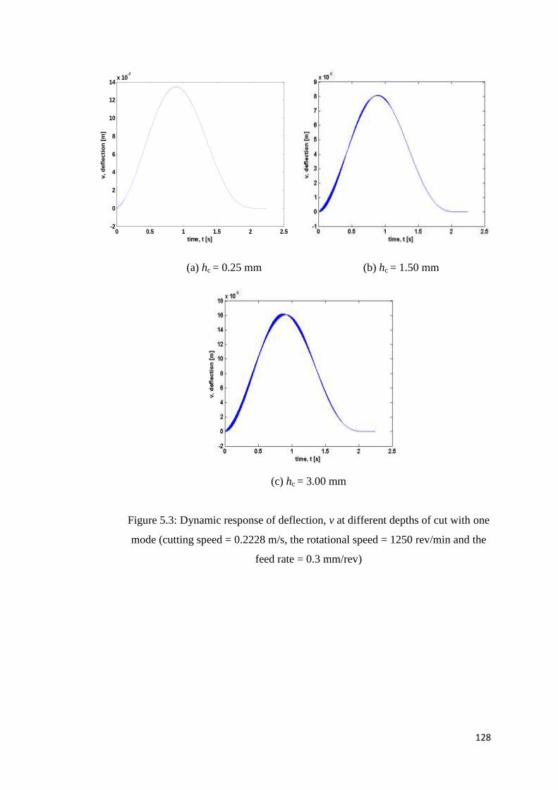
128

(a) hc = 0.25 mm (b) hc = 1.50 mm

(c) hc = 3.00 mm

Figure 5.3: Dynamic response of deflection, v at different depths of cut with one

mode (cutting speed = 0.2228 m/s, the rotational speed = 1250 rev/min and the

feed rate = 0.3 mm/rev)

0 0.5 1 1.5 2 2.5

-2

0

2

4

6

8

10

12

14x 10

-7

v, d

efl

ecti

on

[m

]

time, t [s]

129

(a) hc = 0.25 mm (b) hc = 1.50 mm

(c) hc = 3.00 mm

Figure 5.4: Dynamic response of deflection, w at different depths of cut with one

mode (cutting speed = 0.2228 m/s, the rotational speed = 1250 rev/min and the


130

By using the same parameters in Figure 5.3, the dynamic responses of

deflection, v using two modes are shown in Figure 5.5. Apparently, higher

frequency components seem to have appeared in comparison with one mode.

The high amplitude of oscillation is increased with the increase of number of

modes.

(a) hc = 0.25 mm (b) hc = 1.50 mm

(c) hc = 3.00 mm

Figure 5.5: Dynamic response of deflection, v at different depths of cut with two

modes (cutting speed = 0.2228 m/s, the rotational speed = 1250 rev/min and the


0 0.5 1 1.5 2 2.5

-2

0

2

4

6

8

10

12

14x 10

-7

v, d

efl

ecti

on

[m

]

time, t [s]

131

(a) hc = 0.25 mm (b) hc = 1.50 mm

(c) hc = 3.00 mm

Figure 5.6: Dynamic response of deflection, w at different depths of cut with

two modes (cutting speed = 0.2228 m/s, the rotational speed = 1250 rev/min and

the feed rate = 0.3 mm/rev)

Furthermore, the dynamic response, v obtained using three modes has a similar

pattern as depicted in Figure 5.8. Figure 5.8 (a), 5.8 (b) and 5.8 (c) generate a

same pattern but difference in amplitude due to a higher depth of cut used.

Figure 5.8 (c) appeared to have higher amplitude than Figure 5.8 (a) and 5.8 (b)

since the biggest depth of cut is used. Notice that in the whole Figure 5.8, at half

through time, t the response in Figure 5.8 (c) begins to illustrate a beating

132

phenomenon. Beating phenomenon is when two harmonic motions, with

frequencies and amplitudes close to one another, are added, and then resulting

motion exhibits a phenomenon known as beats. It is different from chatter which

chatter is a harmonic imbalance that occurs between the tool and the work piece

because they are bouncing against each other. Chatter can easily be recognized

by the noise associated with self-excited vibrations. It also can be seen from the

appearance of the chips according to Tlusty (2000). The phenomenon of beating

is often observed in machines, structures and electric houses. For example in

machine and structures, the beating phenomenon occurs when the forcing

frequency is close to the natural frequency of the system (Rao, 1995). The

examples of two harmonic motions are represented as below;

𝑥1 𝑡 = 𝑋 cos 𝜔𝑡 (5.1)

𝑥2 𝑡 = 𝑋 cos 𝜔 + 𝛿 𝑡 (5.2)

where δ is a small quantity and the addition of these motions yields

𝑥(𝑡) = 𝑥1 𝑡 + 𝑥2 𝑡 = 𝑋 [ cos 𝜔𝑡 + cos (𝜔 + 𝛿)𝑡 ] (5.3)

Using the relation

cos 𝐴 + cos 𝐵 = 2 cos 𝐴+𝐵

2 cos

𝐴−𝐵

2 (5.4)

and equation 5.3 can be rewritten as

𝑥 𝑡 = 2𝑋 cos𝛿𝑡

2cos 𝜔 +

𝛿

2 𝑡

This equation is shown graphically in Figure 5.7.

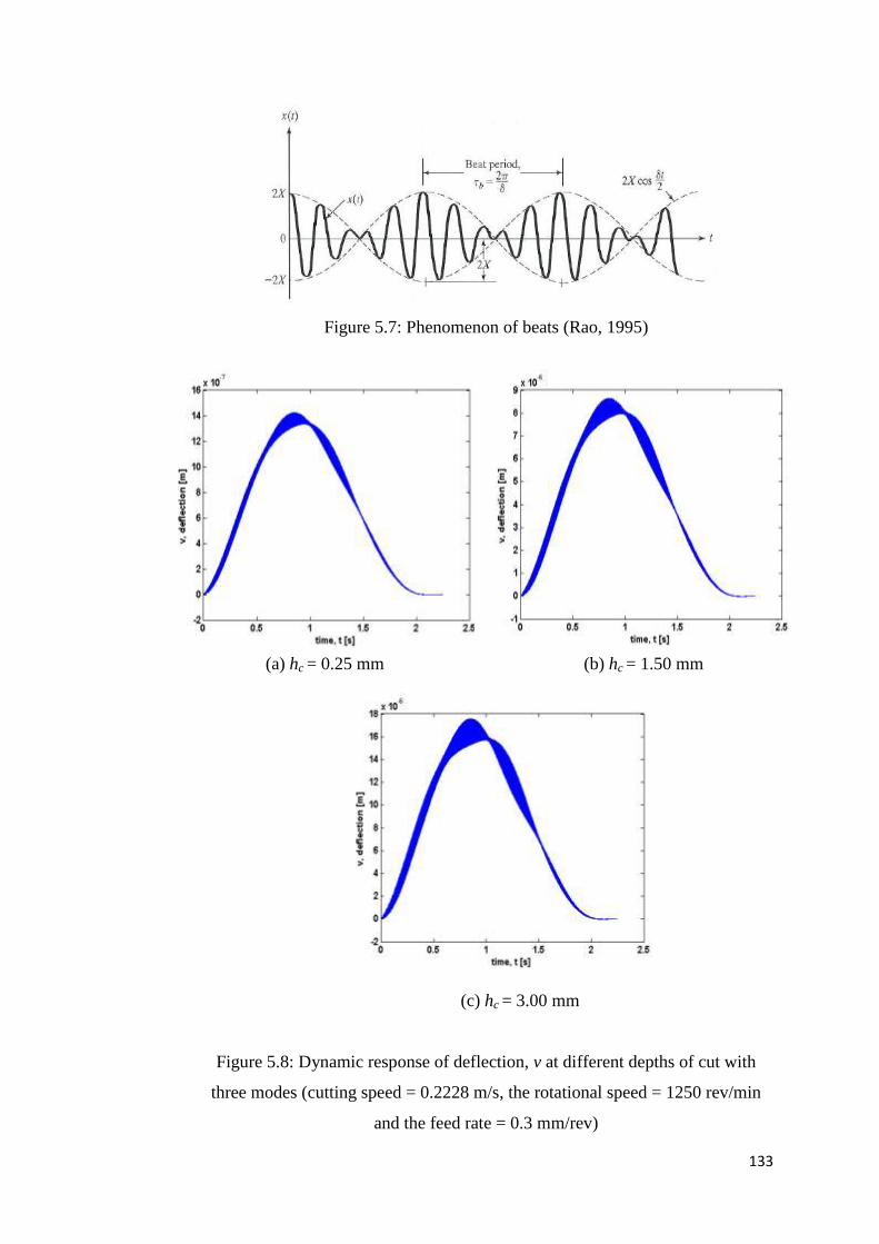
133

Figure 5.7: Phenomenon of beats (Rao, 1995)

(a) hc = 0.25 mm (b) hc = 1.50 mm

(c) hc = 3.00 mm

Figure 5.8: Dynamic response of deflection, v at different depths of cut with

three modes (cutting speed = 0.2228 m/s, the rotational speed = 1250 rev/min

and the feed rate = 0.3 mm/rev)

134

(a) hc = 0.25 mm (b) hc = 1.50 mm

(c) hc = 3.00 mm


three modes (cutting speed = 0.2228 m/s, the rotational speed = 1250 rev/min

and the feed rate = 0.3 mm/rev)

135

A slightly different pattern is produced when four modes are used.

Again, Figure 5.10 (a), 5.10 (b) and 5.10 (c) generate a same pattern but

difference in amplitude due to a higher depth of cut is used. Figure 5.10 (c)

appeared to have higher amplitude than Figure 5.10 (a) and 5.10 (b). At half way

through the time, t the mode shape in Figure 5.10 (c) begins to illustrate a

beating phenomenon.

(a) hc = 0.25 mm (b) hc = 1.50 mm

(c) hc = 3.00 mm


four modes (cutting speed = 0.2228 m/s, the rotational speed = 1250 rev/min and


0 0.5 1 1.5 2 2.5

-5

0

5

10

15

20x 10

-6

v, d

efl

ecti

on

[m

]

time, t [s]

136

(a) hc = 0.25 mm (b) hc = 1.50 mm

(c) hc = 3.00 mm


four modes (cutting speed = 0.2228 m/s, the rotational speed = 1250 rev/min and


137

5.2.2 Effect of Cutting Speed

The next cutting parameter simulated in the dynamic model is the cutting

speed. Figure 5.12 and Figure 5.13 show the dynamic response, v at two

different cutting speeds in order to demonstrate its effect with one mode. The

other cutting parameters are set to be constant which are the depth of cut of 3.00

mm, the rotational speed of 1250 rev/min and the feed rate of 0.3 mm/rev. From

Figure 5.12 (b), high frequency oscillation appeared on top of the nearly static

deflection and the mode illustrates a beating phenomenon. By comparing Figure

5.12 (a) and 5.12 (b), it can be seen that higher-frequency oscillation has bigger

amplitude at a higher cutting speed. The finding is consistent with a conclusion

by Tobias and Fishwick (1958) that a lower cutting speed would suppress

chatter and therefore produce a better surface finish.

(a) cutting speed = 0.2228 m/s (b) cutting speed = 1.4353 m/s

Figure 5.12: Dynamic response of deflection, v at different cutting speeds with

one mode (depth of cut = 3.00 mm, rotational speed = 1250 rev/min and the feed

rate = 0.3 mm/rev)

138


Figure 5.13: Dynamic response of deflection, w at different cutting speeds with

one mode (depth of cut = 3.00 mm, rotational speed = 1250 rev/min and the feed

rate = 0.3 mm/rev)

The same cutting conditions are simulated with two modes and the

results are shown in Figure 5.14 and Figure 5.15. Higher amplitude vibration

becomes more pronounced with more modes. The deflection is skewed to the

weaker support, which is the tailstock. The beating phenomenon is even greater

at a higher cutting speed which is 1.4353 m/s. The results obtained with three

and four modes are similar with two modes as illustrated in Figure 5.16 and

Figure 5.17.

139



two modes (depth of cut = 3.00 mm, rotational speed = 1250 rev/min and the




two modes (depth of cut = 3.00 mm, rotational speed = 1250 rev/min and the


140



three modes (depth of cut = 3.00 mm, rotational speed = 1250 rev/min and the




three modes (depth of cut = 3.00 mm, rotational speed = 1250 rev/min and the


141

A slightly different pattern is produced when four modes (Figure 5.18

and Figure 5.19) are used but the difference in amplitude is due to a high

number of modes included in the simulation. Figure 5.18 (b) appeared to have

higher amplitude with beating phenomenon than Figure 5.18 (a).



four modes (depth of cut = 3.00 mm, rotational speed = 1250 rev/min and the


0 0.5 1 1.5 2 2.5

-5

0

5

10

15

20x 10

-6

v, d

efl

ecti

on

[m

]

time, t [s]

142



four modes (depth of cut = 3.00 mm, rotational speed = 1250 rev/min and the


5.2.3 Effect of Rotational Speed

The last cutting parameter simulated in the dynamic model is the

rotational speed. Figure 5.20 to Figure 5.25 illustrates the results of the effects of

different rotational speeds on dynamic response, v and w, at three different

rotational speeds in order to demonstrate its effect with one mode, two modes,

three modes and four modes. Again, the other cutting parameters are set to be

constant which are the depth of cut is 3.00 mm, the cutting speed is 0.2228 m/s

and the feed rate is 3.00 mm. The results of the effects of different rotational

speeds with one mode are illustrated in Figure 5.20. At lower rotational speed,

the high oscillation only appears at the beginning of the mode shape. There is

not much amplitude difference between the first, second and third modes. The

rotational speed does not seem to have a big effect on the dynamic response

especially on the amplitude of deflection.

143

(a) rotational speed = 230 rev/min (b) rotational speed = 480 rev/min

(c) rotational speed = 1250 rev/min

Figure 5.20: Dynamic response of deflection, v at different rotational speeds

with one mode (depth of cut = 3.00 mm, cutting speed = 0.2228 m/s and the feed

rate = 0.3 mm/rev)

144



Figure 5.21: Dynamic response of deflection, w at different rotational speeds

with one mode (depth of cut = 3 mm, cutting speed = 0.2228 m/s and the feed

rate = 0.3 mm/rev)

There are some differences in oscillation particularly in mode two. When

two modes are used as shown in Figure 5.22, a higher rotational speed is seen to

excite slightly greater high-frequency components. Therefore, increasing the

rotational speed moderately promotes the occurrence of chatter.

145



Figure 5.22: Dynamic response of deflection, v at different rotational speeds

with two modes (depth of cut = 3.00 mm, cutting speed = 0.2228 m/s and the

feed rate = 0.3 mm/rev

146



Figure 5.23: Dynamic response of deflection, w at different rotational speeds

with two modes (depth of cut = 3.00 mm, cutting speed = 0.2228 m/s and the


147

5.3 Elastic Boundary

5.3.1 Introduction

Initially, the assumed boundary conditions were a clamped and pinned to

represent a chuck and a tailstock supports on lathe. Unfortunately, the dynamic

responses, v and w illustrate a small magnitude of deflection which is not

realistic to the actual lathe support (shown earlier in section 5.2). Thus, more

suitable boundary conditions which replicate the actual lathe support should be

adopted to ensure the accuracy of the dynamic response. This new boundary

conditions employed are known as an elastic boundary condition since a chuck

is more suitable to be represented by rotational spring and a tailstock as a linear

spring.

5.3.2 Convergence test

The convergence test has also been performed for the elastic boundary

condition to monitor the occurrence of chatter (up to five modes) and to

determine the appropriate number of modes included in the simulation. The

properties of the shaft (cylindrical metal work piece) used in this convergence

test are length, l = 0.55 m, radius r = 18.5 mm, Young‟s Modulus E = 2.07 x

1011

Pa, and density, 𝝆 = 7817.4 kg/m3 while the cutting parameters used are

2.228 m/s for cutting speed, 1250 rev/min for rotational speed and 0.3 mm/rev

for feed rate. By considering an elastic boundary, its normalized modes are

𝜑𝑛 𝑥 = 𝐶1 cos(𝛽𝑛𝑥) + 𝐶2 sin(𝛽𝑛𝑥) + 𝐶3 cosh(𝛽𝑛𝑥) + 𝐶4 sinh(𝛽𝑛𝑥) (5.1)

where 𝛽𝑛 = [5.777 6.657 13.145 13.685] and 𝜔𝑛 = (𝜆𝑛)2 𝐸𝐼/𝜌𝐴 / 2𝜋𝑙2 (n = 1,

2, 3...) is the natural frequency of the stationary shaft.

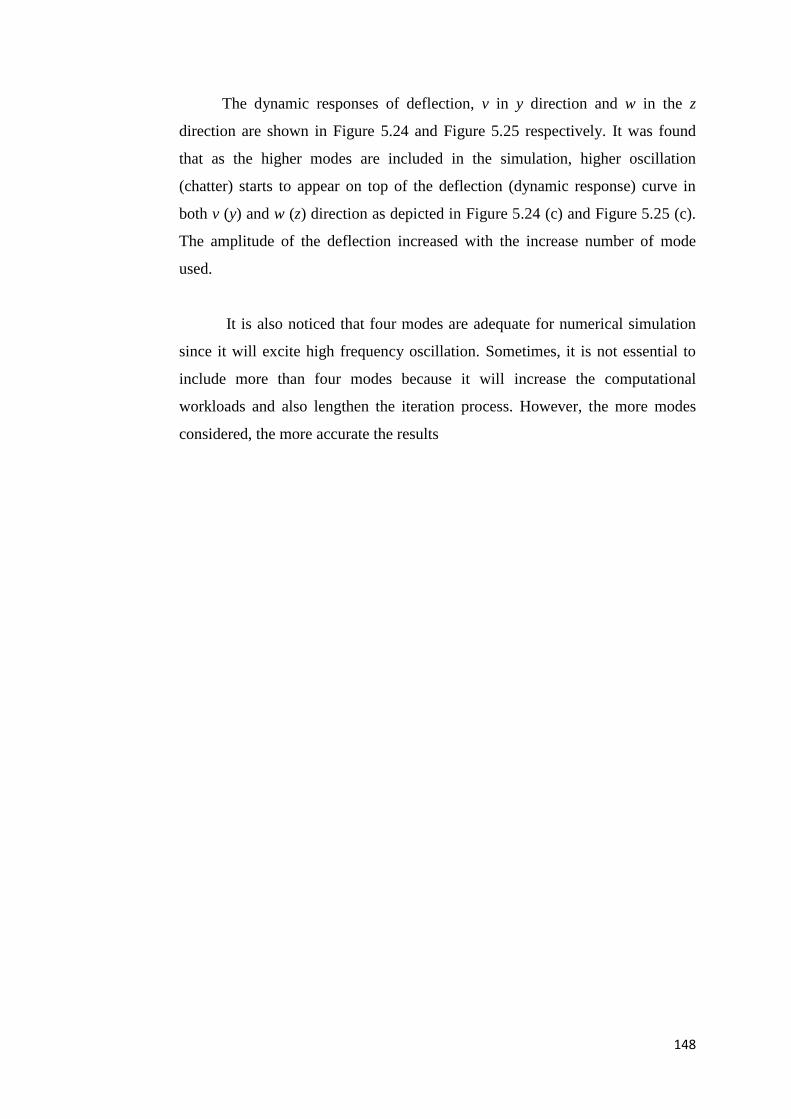
148

The dynamic responses of deflection, v in y direction and w in the z

direction are shown in Figure 5.24 and Figure 5.25 respectively. It was found

that as the higher modes are included in the simulation, higher oscillation

(chatter) starts to appear on top of the deflection (dynamic response) curve in

both v (y) and w (z) direction as depicted in Figure 5.24 (c) and Figure 5.25 (c).

The amplitude of the deflection increased with the increase number of mode

used.

It is also noticed that four modes are adequate for numerical simulation

since it will excite high frequency oscillation. Sometimes, it is not essential to

include more than four modes because it will increase the computational

workloads and also lengthen the iteration process. However, the more modes

considered, the more accurate the results

149

(b) One mode (b) Two modes

(d) Three modes (d) Four modes

(e) Five modes

Figure 5.24: Dynamic response of deflection, v (y direction) with (a) one mode



150

(c) One mode (b) Two modes

(e) Three modes (d) Four modes

(e) Five modes

Figure 5.25: Dynamic response of deflection, w (z direction) with (a) one mode



151

5.3.3 Effect of Depth of Cut

Figure 5.26 illustrates the dynamic responses of deflection, v in y

direction for three different values of depth of cut which is 0.25 mm, 1.50 mm

and 3.00 mm. Besides, the cutting speed, the rotational speed and the feed rate

are constant in which the cutting speed is 2.228 m/s, the rotational speed is 1250

rev/min and the feed rate is 0.3 mm/rev. In elastic boundary conditions, the

cutting speed used is slightly higher as compared with a clamped pinned

boundary. This is done purposely to avoid any intensive computational works

which somehow prolong and complicate the production of results. From the

graph, it shows that an increase in depth of cut will increase the amplitudes and

frequency of oscillation. The 3.00 mm depth of cut is prominent, as the

magnitude of the oscillation becomes bigger. Figures 5.26 (c) and Figure 5.27

(c) indicate that the amplitude of oscillation is the highest among the three

values of depth of cut.

152

(a) hc = 0.25 mm (b) hc = 1.50 mm

(c) hc = 3.00 mm


one mode (1250 rev/min, cutting speed = 2.228 m/s and feed rate is 0.3 mm/rev)

153

(a) hc = 0.25 mm (b) hc = 1.50 mm

(c) hc = 3.00 mm


one mode (1250 rev/min, cutting speed = 2.228m/s and feed rate is 0.3 mm/rev)

154

By using the same parameters in Figure 5.26, the dynamic responses of

deflection, v using two modes are shown in Figure 5.28. Apparently, a different

shape of deflection curve was observed and higher frequency components seem

to have appeared in comparison with one mode. The high amplitude of

oscillation is increased with the increase of number of modes.

(a) hc = 0.25 mm (b) hc = 1.50 mm

(c) hc = 3.00 mm


two modes (1250 rev/min, cutting speed = 2.228 m/s and feed rate is 0.3

mm/rev)

155

(a) hc = 0.25 mm (b) hc = 1.50 mm

(c) hc = 3.00 mm


two modes (1250 rev/min, cutting speed = 2.228 m/s and feed rate is 0.3

mm/rev)

Furthermore, the dynamic response, v obtained using three modes and

four modes have a similar pattern as depicted in Figure 5.30 to Figure 5.33. All

of them generate the same pattern but slightly different in amplitude. For

156

example, Figure 5.30 (c) appeared to have higher amplitude than Figure 5.30 (a)

and 5.30 (b).

(a) hc = 0.25 mm (b) hc = 1.50 mm

(c) hc = 3.00 mm


three modes (1250 rev/min, cutting speed = 2.228 m/s and feed rate is 0.3

mm/rev)

157

(a) hc = 0.25 mm (b) hc = 1.50 mm

(c) hc = 3.00 mm


three modes (1250 rev/min, cutting speed = 2.228 m/s and feed rate is 0.3

mm/rev)

158

(a) hc = 0.25 mm (b) hc = 1.50 mm

(c) hc = 3.00 mm


four modes (1250 rev/min, cutting speed = 2.228 m/s and feed rate is 0.3

mm/rev)

159

(a) hc = 0.25 mm (b) hc = 1.50 mm

(c) hc = 3.00 mm


four modes (1250 rev/min, cutting speed = 2.228 m/s and feed rate is 0.3

mm/rev)

160

5.3.4 Effect of Cutting Speed

The next cutting parameter investigated is cutting speed. Figure 5.34

shows the dynamic response, v at two different cutting speeds for one mode. The

other cutting parameters are set to be constant which are the depth of cut is 3.00

mm, the rotational speed is 1250 rev/min and the feed rate is 0.3 mm/rev. By

comparing Figure 5.34 (a) and 5.34 (b), it can be seen that higher-frequency

oscillation has bigger amplitude at higher cutting speed.


Figure 5.34: Dynamic response of deflection, v at different cutting speed with

one mode (depth of cut = 3.00 mm, rotational speed = 1250 rev/min and feed

rate is 0.3 mm/rev)

161


Figure 5.35: Dynamic response of deflection, w at different cutting speed with

one mode (depth of cut = 3.00 mm, rotational speed = 1250 rev/min and feed

rate is 0.3 mm/rev)

The same cutting conditions are simulated with two modes and the

results are shown in Figure 5.36 and 5.37. The mode shapes have changed when

a higher number of modes are used. Similar pattern and amplitude of vibration

were produced for different cutting speeds. Higher amplitude vibration becomes

more pronounced with more modes. The deflection is skewed to the weaker

support, which is the tailstock. The beating phenomenon is even greater at a

higher cutting speed which is 1.4353 m/s. The results obtained with three and

four modes are similar with two modes as illustrated in Figure 5.38, 5.39, 5.40

and 5.41.

162



two modes (depth of cut = 3.00 mm, rotational speed = 1250 rev/min and feed

rate is 0.3 mm/rev)



two modes (depth of cut = 3.00 mm, rotational speed = 1250 rev/min and feed

rate is 0.3 mm/rev)

163



three modes (depth of cut = 3.00 mm and rotational speed = 1250 rev/min and

feed rate is 0.3 mm/rev)



three modes (depth of cut = 3.00 mm, rotational speed = 1250 rev/min and feed

rate is 0.3 mm/rev)

164



four modes (depth of cut = 3.00 mm, rotational speed = 1250 rev/min and feed

rate is 0.3 mm/rev)



four modes (depth of cut = 3.00 mm, rotational speed = 1250 rev/min and feed

rate is 0.3 mm/rev)

165

5.3.4 Effect of Rotational Speed

The final cutting parameter examined is rotational speed. The results of

the dynamic response, v at different rotational speeds are illustrated in Figure

5.42. In the simulation works, the other cutting parameters are set to be constant

which are the depth of cut is 3.00 mm, the cutting speed is 2.228 m/s and the

feed rate is 0.3 mm/rev. It is observed that there is not much amplitude

difference between the first, second and third modes. A similar pattern is also

produced for all rotational speed. The rotational speed does not seem to have a

big effect on the dynamic response especially on the amplitude of vibration.

(a) 230 rev/min (b) 480 rev/min

(c) 1250 rev/min

Figure 5.42: Dynamic response of deflection, v at different rotational speed with

one mode (depth of cut = 3.00 mm, cutting speed = 2.228 m/s and feed rate =

0.3 mm/rev)

166


(c) 1250 rev/min

Figure 5.43: Dynamic response of deflection, w at different rotational speed with

one mode (depth of cut = 3.00 mm, cutting speed = 2.228 m/s and feed rate =

0.3 mm/rev)

A different deflection curve has been produced when a higher number of

modes are used. Figures 5.44 to 5.49 illustrate the deflection, v at depth of cut,

3.00 mm with two, three and four modes and these graphs demonstrate the effect

of including more modes. There are some differences in amplitude of vibration

167

particularly in mode three and four. When three modes are used as shown in

Figure 5.46, a higher number of modes used is seen to excite slightly greater

amplitude of vibration. Therefore, increasing the number of modes moderately

promotes the occurrence of chatter. The deflection, w obtained with three and

four modes are shown in Figure 5.49 and 5.51 for comparison. Adding more

modes does not change w as much as v.


(c) 1250 rev/min


two modes (depth of cut = 3.00 mm, cutting speed = 2.228 m/s and feed rate =

0.3 mm/rev)

168


(c) 1250 rev/min


two modes (depth of cut = 3.00 mm, cutting speed = 2.228 m/s and feed rate =

0.3 mm/rev)

169


(c) 1250 rev/min


three modes (depth of cut = 3.00 mm, cutting speed = 2.228 m/s and feed rate =

0.3 mm/rev)

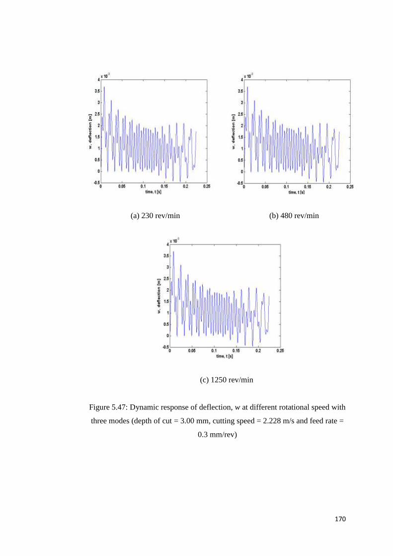
170


(c) 1250 rev/min


three modes (depth of cut = 3.00 mm, cutting speed = 2.228 m/s and feed rate =

0.3 mm/rev)

171


(c) 1250 rev/min


four modes (depth of cut = 3.00 mm, cutting speed = 2.228 m/s and feed rate =

0.3 mm/rev)

172


(c) 1250 rev/min


four modes (depth of cut = 3.00 mm, cutting speed = 2.228 m/s and feed rate =

0.3 mm/rev)

173

5.2.3 Clamped Pinned (Composite work piece)

A simulation work has also been done for clamped pinned boundary

condition on composite work piece. It is done as a preliminary study to

investigate several cutting parameters such as cutting, depth of cut, rotational

speed and the feed rate on turned composite. The geometric and material

properties of the work piece are length, l = 0.5 m, radius r = 19 mm, Young‟s

Modulus E = 36.75 x 109 Pa, and density, 𝝆 = 882 kg/m

3 while the cutting

parameters used are 0.2228 m/s for cutting speed, 0.25 mm for the depth of cut,

1250 rev/min for rotational speed and 0.3 mm/rev for the feed rate. The

numerical results of the dynamic response of deflection, v and w in both y and z

direction under these cutting parameters are shown in Figures 5.50 and 5.51

below.

It can be seen that a similar deflection curve pattern is formed. At

smaller depth of cut (0.25 mm), low frequency oscillations begin to appear thus

indication of chatter presence. Similar to the metal work piece, the simulated

deflection is not symmetrical due to the clamped pinned boundary condition. If a

different depth of cut is being used for example a bigger depth of cut (3.00 mm),

the result obtained will be the same as with metal work piece simulated earlier

where higher frequency oscillations will be generated on top of the static

deflection. Notice that the amplitude of the dynamic response, v and w for both

of the depth of cuts (0.25mm and 3.0mm) is slightly bigger than metal work

piece. This is true because of the nature of composite material itself is

inhomogeneous.

174

Figure 5.50: Dynamic response of deflection, v at one mode (depth of cut = 0.25

mm, cutting speed = 0.2228 m/s, rotational speed = 1250 rev/min and feed

rate = 0.3 mm/rev)

Figure 5.51: Dynamic response of deflection, w at one mode (depth of cut = 0.25

mm, cutting speed = 0.2228 m/s, rotational speed = 1250 rev/min and feed rate =

0.3 mm/rev)

175

Figure 5.52: Dynamic response of deflection, v at one mode (depth of cut = 3.0


rate = 0.3 mm/rev)

Figure 5.53: Dynamic response of deflection, w at one mode (depth of cut = 3.0


rate = 0.3 mm/rev)

176

5.3 Vibration Test During Turning Operation

As mentioned earlier in Chapter 4, due to the limitation of the equipment

in performing vibration testing during turning operation at the University of

Liverpool, the results from the other collaborator group from Dalian University

of Technology (DUT) in China are employed to validate the dynamic model

established.

The cutting parameters used during the turning operation are shown in

Table 5.1. The rotating speed, feed rate and depth of cut are carefully chosen in

different values consistent with the previous numerical simulations under

different cutting conditions. The geometric and material properties of the work-

piece are length, l = 0.5 m, Young‟s Modulus, E = 2.07 x 1011

Pa, and material

density, 𝝆 =7850 kg/m3.

Table 5.1: Cutting parameters and work piece characteristics used during turning

operation (Han et al, 2012)

Experiment

Rotational

speed

(rev/min)

Depth of cut,

ap (mm)

Feed rate,

f (mm/rev)

Diameter,

D (mm)

1 1250 1.5 0.3 36.5

2 1000 3.0 0.2 35.0

Figure 5.54 shows the photograph of the machined cylindrical metal work piece

for experiment 1. The dynamic responses of the shaft (cylindrical metal work

piece) in y and z directions are measured at the position being machined during

the turning process as depicted in Figure 5.55.

177

Figure 5.54: The being machined work piece of experiment 1 (Han et al, 2012)

Figure 5.55: Deflections in time domain of experiment 1 (Han et al, 2012)

178

A higher depth of cut and a smaller feed rate are used in experiment 2 to

observe the effect of varying the cutting parameters. The machined cylindrical

metal work piece is shown in Figure 5.56, in which the phenomena of chatter

can be clearly seen in the middle of the cylindrical metal work piece (marked as

a dotted white line). Chatter is large amplitude irregular vibration, happening

during machining shown in the large dynamic response. Moreover, higher

oscillation appears in the dynamic response of the time domain as illustrated in

Figure 5.57.

Figure 5.56: The being machined work piece of experiment 2 shown chatter

occurrence (Han et al, 2012).

179

Figure 5.57: Deflections in time domain of experiment 2 (Han et al, 2012).

In comparison of the dynamic responses, v and w of the work piece, it

can be seen that the deformation patterns are fairly similar between the

experiment and the developed model. However, the measured deflections are

greater than the developed model. It is believed that the dynamic model

developed is stiffer. Examining all the numerical results, it may be concluded

that the predicted and measured patterns of time histories of work piece

vibration agree fairly well but the magnitudes are not so close to each other, in

particular when the large vibration (chatter) is excited during experiments.

Further improvement to the model is likely to come from a more accurate

representation of the chuck and tail stock boundaries.

180

5.6 Chapter Summary

This chapter presents numerical simulation work of vibration of a metal

work piece being turned. The work piece is modeled as a rotating Rayleigh

beam and the cutting forces as three directional moving loads with regenerative

chatter mechanism. The moving cutting forces with regenerative chatter

introduce time delay in the dynamic model. The effects of depth of cut, cutting

speed and rotational speed of the cutter on vibration and chatter occurrence are

examined. The effect of using several numbers of modes is also investigated.

The results for all three cutting parameters simulated when an elastic

boundary is considered generate a slightly different oscillation compared with

clamped pinned boundary assumed earlier. The oscillations are much higher

when elastic boundary is considered. The results are in line with the actual work

piece where the chuck and tailstock also deform. The amplitude of vibration as

well increases when the number of modes used in the simulation increases.

Similar to clamped pinned boundary, four modes are sufficient and hence used

during the numerical simulation. It is necessary to include higher modes as it

will cover high frequency oscillation. The more modes considered, the more

accurate the results; but at certain points it is not necessary to include more than

four modes.

For both clamp pinned and elastic boundary conditions, an increase in

depth of cut will increase the amplitudes and frequency of oscillation. The

response at 3.00 mm depth of cut is significant as the magnitude of the

oscillation becomes bigger. Most of the high amplitude of oscillation increases

with the increase of number of modes. Moreover, higher cutting speed will

generate a higher frequency oscillation hence bigger amplitude is obtained. On

the other hand, for the effect of different rotational speed, it can be concluded

that there is not much amplitude difference between the first, second and third

modes. There are some differences in amplitude of vibration particularly in

modes three and four. Therefore, increasing the number of modes moderately

promotes the occurrence of greater response in simulation.

181

From the experiment done by the collaborating group in China, it can be

seen that the deformation patterns are fairly similar between both the experiment

and the developed model. However, the measured deflections are smaller than

the developed dynamic model. It is believed that the theoretical model with

clamped pinned boundary is much stiffer since the chuck is represented by a

clamped boundary and the tail stock support is represented by a pinned

boundary. In contrast, from the results gained when an elastic boundary is

considered, the simulated deflection magnitude is bigger than the measured

deflection during experiment. It can be concluded that the predicted and

measured patterns of time histories of work piece vibration agree fairly well

when an elastic boundary conditions are considered in the simulation works of

the developed dynamic model.

In conclusion a dynamic model for a rotating Rayleigh beam subjected to

a three directional moving cutting forces with regenerative chatter effect is

successfully established.

182

Chapter 6

Analysis and Discussion

6.1 Parametric Studies

6.1.1 Clamped Pinned (Metal work piece)

The first simulation work done is to monitor the occurrence of chatter

(up to five modes) and to determine the appropriate number of modes used in

the simulation. Initially the boundary condition used was a clamp-pinned

boundary as the work piece is held in chuck at one end and the other end was

pinned down by a tailstock. This is also the boundary condition considered in

papers on vibration in turning operation by other researchers. From the results

shown earlier (Figure 5.1 (d) and Figure 5.2 (d)), when higher modes are used in

the simulation, higher oscillation (chatter) starts to appear on top of the

deflection (dynamic response) curve in both v (y) and w (z) directions. It is

necessary to simulate higher modes as they will cover high frequency oscillation

and the dynamic responses settle at four modes.

It is also observed that four modes are satisfactory to be used in the

parametric studies since high frequency oscillation is present on the top of the

deflection curve showing chatter occurrence. Furthermore, it also demonstrates

183

the effectiveness of the dynamic model developed in detecting chatter. It is

necessary to include higher modes in the simulation as the more modes

considered, the more accurate the results. However, at certain points more than

four modes are not necessary as one of the aims of the numerical simulation is to

define the appropriate number of modes and four modes are defined to be a

starting point where the mode shape start to converge indicative of a stable

system. Furthermore, more than four modes will produce similar results but if

more than four modes are used, it will have more computational workloads. In

addition, the deflection curve produced also shows the dynamic model

developed works successfully at the initial stage since it truly represents the

behaviour of the work piece during turning operation in which the deflection is

generated as predicted.

The developed dynamic model is also simulated to investigate the effects

of three main cutting parameters; the depth of cut, the cutting speed and the

rotational speed on the chatter occurrence.


From the results illustrated earlier (Figure 5.3), it is noticed that the increase of

depth of cut used during simulation results in the increase of amplitudes and

frequency of oscillation. This condition is in fact reflecting the actual turning

process where an increase of depth of cut will increase the chance of the

occurrence of chatter on turned work piece. The 3.00 mm depth of cut used

shows two features, a nearly static deflection and high frequency oscillations

start to appear at the same time. The presence of chatter appears at the beginning

of pinned support. In addition, the deflection curves produced are not

symmetrical due to the clamped pinned boundary assumption earlier. The

clamped support is much stiffer than the other pinned support. However, when

the same parameters are used with a slightly higher mode; two, higher vibration

magnitude appears. This is because higher modes will cover higher frequency

oscillation during numerical simulation. As the number of modes increases, the

184

higher oscillation develops. A similar pattern is obtained for the dynamic

response, v using three modes and four modes but with slightly higher vibration

magnitude. The use of higher modes results in higher amplitude oscillation and a

beating phenomenon also starts to develop. The beating phenomenon occurs

when the forcing frequency is close to the natural frequency of the system. This

phenomenon is often observed in machinery, structures and electric power

houses.

6.1.1.2 Effect of Cutting Speed

The next cutting parameter simulated in the dynamic model is the cutting

speed in which the effect of two different cutting speeds is examined with one

mode. Only two values of cutting speeds are simulated because it took more

than 24 hours to run for each mode shape before the analysis stops for the

smallest cutting speed (0.0062 m/s). From the results shown (Figure 5.5 (b)),

high frequency oscillation is observed on top of the nearly static deflection due

to the use of high cutting speed. Since the depth of cut used is quite high (3.00

mm), it promotes frequency oscillation to increase for higher cutting speed used.

If the two graphs from Figure 5.5 (a) and 5.5 (b) are compared, it can be seen

that higher-frequency oscillation has bigger amplitude at a higher cutting speed.

A lower cutting speed would suppress chatter as mentioned by Tobias and

Fishwick (1958) and this is true only if smaller values of depth of cut are used.

When the same cutting conditions are simulated with two modes (Figure

5.6), higher amplitude vibration becomes more prominent with more modes. By

simulating higher modes, higher frequency oscillation is found. Both of the

dynamic response (v and w) should be in the middle of the work piece, but since

the work piece has its own inertia, the deflection is skewed to the weaker

support, which is the tailstock. The beating phenomenon is even greater at a

higher cutting speed of 1.4353 m/s. It occurs when the excitation frequency is

close to the natural frequency of the system and the cutting speed influences the

excitation frequency. The results obtained with three and four modes are similar

185

to two modes since from two modes, it already shows convergence of

displacement in both directions, y and z.

6.1.1.3 Effect of Rotational Speed

The rotational speed does not seem to have a big impact on the dynamic

response of the shaft. At lower rotational speed, the high oscillation only appears

at the beginning of the mode shape (Figure 5.20). Small difference of amplitude

is noticed between the first, second and third mode but slight dissimilarity is

observed in oscillation particularly in two modes. When higher modes are used

(two modes), higher rotational speed excites slightly greater high-frequency

components. It is because dynamic response starts to settle and converges and

hence increasing the rotational speed moderately promotes the occurrence of

chatter.

Since there is no consideration of deflection, w in the instantaneous

depth of cut formula, h, the deflection, w in the z direction has a very similar

pattern for different depth of cut, cutting speed and rotational speed with one

mode and two modes only. In addition, the use of higher modes (bigger than

two) during numerical simulation brought in some local features but the pattern

of dynamic response remains somewhat similar. It is because the dynamic

response starts to settle and converges at four modes. In conclusion, for the

effect of rotational speed at 3.00 mm depth of cut, including more modes does

not change deflection, w in z direction as much as deflection, v in y direction.

6.1.2 Elastic Boundary (Chuck tailstock – Metal work

piece)

Since there are some problems encountered using the clamped pinned

boundary condition assumed earlier which led to some discrepancies in metal

work piece natural frequencies and mode shapes, a suitable boundary should be

186

considered, in this case an elastic boundary condition because in practice both

supports (chuck and tailstock) are actually flexible. This boundary condition is

then employed in the developed dynamic model (Chapter 3) and the simulated

numerical results (Chapter 5).

The convergence test has been performed initially for the elastic

boundary condition. It is done to monitor the occurrence of chatter (up to five

modes) and to determine the appropriate number of modes included in the

simulation. The properties of the shaft (cylindrical metal work piece) used is

similar to the one that is being used for a clamp pinned boundary. The only

difference is the cutting parameters used especially for cutting speed where a

slightly higher value is used (2.228 m/s). A higher value is selected in order to

avoid longer computational workloads. The classical normalizes modes are used

for an elastic boundary (shown in Equation 3.61).

From the results shown earlier, it can be seen that as the higher modes are

included in the simulation, higher oscillation (chatter) starts to appear on top of

the deflection (dynamic response) curve in both v (y) and w (z) direction. It is

required to simulate higher modes as this will cover high frequency oscillation.

The amplitude of the deflection as well increases when the number of modes

used in the simulation increases. It is also observed that four modes of the shaft

are adequate. It is necessary to include higher modes as it will stimulate high

frequency oscillation. The more modes are considered, the more accurate the

results are but it is also time consuming.


Same values of depth of cut are used which are 0.25 mm, 1.50 mm and

3.00 mm and a same constant value of the cutting speed and the rotational speed

are employed. From the results it can be seen that an increase in depth of cut

will increase the amplitudes and frequency of oscillation. The 3.00 mm depth of

cut is significant as the magnitude of the oscillation becomes bigger. The same

187

parameters are simulated for two modes and it appears that a different shape of

deflection curve is observed and higher frequency components seem to have

appeared in comparison with one mode. Most of the high amplitude of

oscillation is increased with the increase of number of modes. A similar pattern

of deflection curve is also obtained but slightly different in amplitude for three

and four modes. Higher amplitude was obtained when a higher depth of cut is

used.

6.1.2.2 Effect of Cutting Speed

The two different cutting speeds are next simulated to demonstrate its

effect with one mode. A constant value of depth of cut (3.00 mm) and rotational

speed (1250 rev/min) were employed. From the results it appears that higher-

frequency oscillation has bigger amplitude at a higher cutting speed. The same

cutting conditions are also simulated for two modes and it can be seen that the

mode shapes have changed when a higher number of modes were used. Similar

pattern and amplitude of vibration were produced for different cutting speed and

higher amplitude vibration becomes more distinct with more modes. The

deflection is slanted to the weaker support, which is the tailstock. The beating

phenomenon is even greater at a higher cutting speed (1.4353 m/s). The results

obtained for three and four modes are similar with two modes.

6.1.2.3 Effect of Rotational Speed

There are different rotational speeds simulated which are 230 rev/min,

480 rev/min and 1250 rev/min. It is observed that a similar pattern is generated

for all rotational speeds and there is not much amplitude difference between the

first, second and third modes. It can be said that a variation of rotational speed

does not seem to have a big effect on the dynamic response especially on the

amplitude of vibration. However, a different pattern has been obtained when a

higher number of modes are used. There are some differences in amplitude of

188

vibration particularly in modes three and four. A higher number of modes (three

or more modes) are seen to stimulate slightly greater amplitude of vibration.

Therefore, increasing the number of modes moderately promotes the occurrence

of chatter. In addition, adding more modes does not change w as much as v.

6.2 Validation Between Numerical and Experimental

Results

The experiments were conducted with a collaborator at Dailan University

of Technology (DUT) in China and the results were employed to validate the

dynamic model established. Variation of cutting parameters including the

rotating speed, feed rate and depth of cut are carefully chosen in different values

consistent with the previous numerical simulations under different cutting

conditions in order to investigate the effect of varying the cutting parameters.

The phenomena of chatter can be clearly seen at the middle of the cylindrical

metal work piece. Moreover, higher oscillation appears in the dynamic response

of the time domain.

It can be observed that the deformation patterns are fairly similar

between both the experiments and the developed model of clamped pinned and

elastic boundary conditions. In the beginning, the theoretical deflections of

clamped pinned are greater from the experiment as compared with the

developed clamped pinned dynamic model. It might be due to the fact that the

initial boundary condition assumed earlier in the theoretical dynamic model is

much stiffer at the chuck and more flexible at the tail stock support. In contrast,

from the results gained when an elastic boundary is employed, the simulated

theoretical deflection magnitude is slightly greater than the measured deflection

during experiment. The results are more realistic since both the chuck and

tailstock were assumed to be flexible support. Practically the work piece and

cutting tool suffer from deflection. It can be concluded that the predicted and

measured patterns of time histories of work piece vibration agree fairly well

when an elastic boundary conditions are considered in the simulation works of

189

the developed dynamic model. Note that in Table 6.1 below both of the x-axis of

theoretical and experiment graphs represent the moving cutting coordinates. For

the theoretical x-axis, it can be calculated by dividing the length of the work

piece over cutting speed while in the experiment x-axis, it is simply the length of

the work piece subtracted with the product of cutting speed and time.

Table 6.1: Comparison between theoretical and experimental of dynamic

responses at both v and w

Theoretical (Chuck-tailstock) Experimental

Dynamic response at v in y direction

Dynamic response at w in z direction

Dynamic response at v in y direction

Dynamic response at w in z direction

190

Chapter 7

Conclusion and Future Work

7.1 Summary of Findings of the Investigation

This thesis presents a study of vibration of work pieces in turning

operation modelled as a rotating beam with clamped pinned and elastic supports

subjected to three directional moving loads with regenerative chatter

mechanism. From the literature reviews done, some of the limitation of previous

chatter models (manufacturing engineer models) are that none of them consider

moving loads in their dynamics model. Moving loads (cutting forces) should be

considered because they are variable in both space and time as the cutter moves

along the work piece (a large number of the engineering structures are subjected

to time and space varying loads). The moving cutting forces also consider the

regenerative chatter effect.

In addition, most studies of dynamic model of turning operation

previously have generally assumed the work piece to be rigid and no

deformation of work piece is considered. However, in practice the work piece

does have deformation when there is an external force exerting on it. Such

deformation will change the chip thickness and have an effect on the critical

chip thickness and dynamic stability. Although work piece vibrations impact

191

both cutting instability and product quality including surface finish, most models

developed for investigating surface roughness do not consider work piece

vibrations at all. Therefore, in this project, the research is focussed on

developing a new mathematical model considering both the work piece and

cutting tools as flexible. Besides, it is also concluded that the most significant

factors contributing to the surface finish quality are the cutting parameters which

are the cutting speed, depth of cut and feed rate. One should be more careful in

considering the cutting condition used is within recommended range to prevent

unstable cutting condition.

The development of the dynamic models was initiated by identifying

suitable boundary conditions. The energy method is then employed since the

energy of a vibrating system of a turning process is partly potential and partly

kinetic. The equation of motion of vibration of a rotating work piece in turning

operations is then derived using Lagrange‟s equations. Three directional moving

cutting forces with regenerative chatter mechanism is next included in the

dynamic model developed. The improved dynamic model is later generated by

adapting Insperger‟s cutting force model. Lastly, the cutting tool equation of

motions for new improved dynamic model is also established and computed in

Matlab software. A method to analyse chatter is also established by utilizing a

dynamic transient response analysis. Runge-Kutta method has been used

initially but since Runge-Kutta always depends on the initial conditions, a Delay

Differential equation was selected to replace the Runge-Kutta method since it is

a self generated algorithm where the time step will be automatically recognized.

In order to investigate the effect of the cutting parameters, the numerical

simulation work is performed to observe the influence of these cutting

parameters on the chatter occurrence. Numerical results of the deflection of the

beam for these three different cutting parameters (depth of cut, cutting speed and

rotational speed) are obtained. It is found that the cutting force model of

regenerative chatter which introduces time delay in a dynamic model leads to an

interesting dynamic behaviour in the vibration of rotating beams and a sufficient

number of modes must be included to sufficiently represent the dynamic

behaviour. The effects of depth of cut, the cutting speed and rotational speed on

192

the vibration and chatter occurrence are examined and obtained. Simulated

numerical examples are presented as well.

During the simulation work, two types of boundary conditions are

considered; clamped pinned and chuck tailstock (elastic boundary). The results

for all three cutting parameters are simulated when an elastic boundary is

considered producing a slightly different oscillation as compared with a clamped

pinned boundary assumed earlier. The oscillations are much higher when elastic

boundary is considered. The results are in line with the actual practice where the

work piece suffers from deformation. The amplitude of vibration increases as

well when higher numbers of modes are used in the simulation. Similar to

clamped pinned boundary, four modes are sufficient and hence used during

numerical simulation. It is necessary to include higher modes as it will excite

high frequency oscillation. The more modes considered, the more accurate the

results; but it is not necessary to include more than four modes.

These three different cutting parameters are vital and definitely influence

the dynamic responses of deflection in the y and z directions. The depth of cut is

seen to be the most influential on the magnitude of the deflection. For both

clamp pinned and elastic boundary conditions, an increase in depth of cut will

increase the amplitudes and frequency of oscillation. The 3.00 mm depth of cut

is significant as the magnitude of the oscillation becomes bigger. Most of the

high amplitude of oscillation increased with the increase of number of modes.

Moreover, higher cutting speed will generate a higher-frequency oscillation

hence bigger amplitude is obtained. The mode shape pattern changes when a

higher number of modes are used. Higher amplitude vibration becomes more

pronounced with more modes. Besides, for the effect of different rotational

speed, there is not much amplitude difference between the first, second and third

modes. A similar pattern of mode shapes is gathered for all rotational speeds.

The rotational speed does not seem to have a big influence on dynamic response

especially on the amplitude of vibration. In addition, a different pattern has been

produced when a higher number of modes are used. There are some differences

in amplitude of vibration particularly in mode three and four. When three modes

are used, a higher number of modes used are seen to excite slightly greater

193

amplitude of vibration. Therefore, increasing the number of modes moderately

promotes the occurrence of chatter.

Several turning experiments are conducted to demonstrate the existence

of vibration and chatter during machining operations. The deformation patterns

obtained are reasonably comparable between both the experiment and the

developed model. However, the measured deflections are larger from the

experiment. It is due to the theoretical model developed is stiffer since the chuck

is represented by a clamped boundary and the tail stock support is represented

by a simple support. On the contrary, the simulated deflection magnitude gained

when an elastic boundary is considered produces a slightly greater magnitude of

deflection to the measured deflection during experiment. It can be concluded

that the predicted and measured patterns of time histories of work piece

vibration agree fairly well when an elastic boundary conditions are considered in

the simulation work of the developed dynamic model. These have been both

theoretically predicted and experimentally validated.

Lastly, a dynamic model for a rotating Rayleigh beam subjected to a

three directional moving cutting forces with regenerative chatter effect is

successfully established. The use of established information from the parametric

studies on turning operation can be of assistance to the operators in choosing the

optimum acceptable turning cutting conditions that will prevent instability and

consequent deterioration of the quality of the turned components.

7.2 Contribution to New Knowledge

The main original contributions delivered by this research are listed as

follows:

7.2.1 The mathematical model developed considered work piece and cutting

tools as a flexible work piece and flexible cutting tools. Without doubt,

this dynamic model of vibration of work piece in turning operation is

194

more realistic than previous ones as the dynamic model has multiple-

degrees-of-freedom and considers the vibration of the cutter with

regenerative chatter. In reality the work piece does have deformation

when there is an external force exerting on it. Such deformation will

change the chip thickness and have an effect on the critical chip

thickness of stability.

7.2.2 The work piece is modelled as a rotating Rayleigh beam and the cutter

provides a three-dimensional moving load with time delay based on the

introduction of regenerative chatter mechanism.

7.3.3 Elastic boundary condition is employed in the developed mathematical

model to mimic the actual chuck and tailstock support for the work piece

on lathe machines.

7.3 Recommendations for Further Investigation

The following suggestions can be made for future research:

7.3.1 Acquire better mechanism of sensing to capture deflection during turning

process since the previous laser sensor used was too noisy to capture the

expected natural frequencies and mode shapes. The used of laser

displacement sensor is more practical to mount in measuring the

vibration of the work piece during turning operation.

7.3.2 Performing experimental modal analysis on composite work pieces since

one of the initial aim of this research is to reduce vibration and chatter

during turning operation by means of numerical and experimental

studies. These can be achieved by pursuing several main objectives of

this research. First is to understand what affect the vibration and noise

during turned metal in a quantitative manner and then find ways of

alleviating this problem by parametric studies.

195

7.3.3 Next is the development of the mathematical model which then will be

validated against the experimental results. The validated model will be

used to simulate structural modifications in order to identify means of

design improvements and vibration reduction.

7.3.4 Machine the composite work pieces using turning process as this

research is emphasis on turning process.

7.4 List of Publications

7.4.1 Journal Paper

Han, X., Ouyang, H., Wang, M., Hassan, N., Mao, Y., 2012, Self-

excited Vibration of Workpieces in a Turning Process, Proc.

IMechE Part C: J. Mechanical Engineering Science, 226(8) 1958-

1970.

7.4.2 Conference Paper

Hassan, N., Ouyang, H., 2011, A Dynamic Chatter Model For

Turning Processes With A Moving Regenerative Cutting Force,

International Conference on Structural Engineering Dynamics,

Tavira, Portugal.

196

References

Al-Regib, E., Ni, J., Lee, S. H., 2003, Programming spindle speed variation for

machine tool chatter suppression, International Journal of Machine Tools &

Manufacture, 43 (12): 1229-1240.

Altintas, Y., 2000, Manufacturing Automation: Metal Cutting Mechanics,

Machine Tool Vibrations, and CNC Design, Cambridge University Press,

Cambridge.

Altintas, Y., Chan, P. K., 1992, In process detection and suppression of chatter

in milling, Int J Mach Tools Manuf, 32, 329–347.

Argento, A., Morano, H. L., 1995, A Spinning Beam Subjected to a Moving

Deflection Dependent Load. 2: Parametric Resonance, J. Sound Vib., 182 (4)

, pp. 617–622.

Argento, A., Scott, R. A., 1992, Dynamic Response of a Rotating Beam

Subjected to an Accelerating Distributed Surface Force, J. Sound Vib., 157

(2), pp. 221–231.

Azouzi, R., Guillot, M., 1997, On-line prediction of surface finish and

dimensional deviation in turning using neural network based sensor fusion,

International Journal of Machine Tools and Manufacture, 37 (9), pp. 1201–

1217.

http://www.sciencedirect.com/science/journal/08906955/37/9

197

Basavarajappa, S., Chandramohan, G., Rao, K. V. N., Radhakrishanan, R.,

Krishnaraj, V., 2006, Turning of particulate metal matrix composites –

review and discussion, Proc. IMechE, Vol. 220, pp.1189-1203.

Bhatnagar, N., Ramakrishnan, N., Naik, N. K., Komandur, R., 1995, On the

machining of fiber reinforced plastic (FRP) composite laminates, Int. J.

Mach. Tools Manufacturing, 35 (5), pp.701-716.

Birhan, I., 2008, Experimental investigations of surface roughness in orthogonal

turning of unidirectional glass-fiber reinforced plastic composites, The

International Journal of Advanced Manufacturing Technology, 37 (1-2), pp

42-48.

Budak, E., 2006, Analytical Methods for High Performance Milling-Part II:

Dynamics and Stability, International Journal of Machine Tools &

Manufacture, 46, pp. 1489-1499.

Budak, E., Wiercihroch, M., 2001, Sources of nonlinearities, chatter generation

and suppression in metal cutting, Philosophical Transactions of the Royal

Society of London, Part A, 359, pp. 663-693.

Chandiramani, N.K., Pothala, T., 2006, Dynamics of 2-DOF regenerative chatter

during turning, J. Sound Vib., 290, p. 448–464.

Chen, C. K., Tsao, Y. M., 2006, A stability analysis of regenerative chatter in

turning process without using tailstock, International Journal of Advanced

Manufacturing Technology, 29, pp. 648-654.

Chen, C. K., Tsao, Y. M., 2006, A stability analysis of turning a tailstock

supported flexible work piece, International Journal of Machine Tools &

Manufacturing, 46, pp. 18-25.

Chen, L. W., Ku, D. M., 1997, Dynamic stability of a cantilever shaft-disk

system, ASME Journal of Vibration and Acoustics, 181 (1), pp. 326-329.

http://link.springer.com/journal/170



198

Chen, M., Knopse, C. R., 2007, Control approaches to the suppression of

machining chatter using active magnetic bearings, IEEE Trans Control

Systems Technology, 15 (2), pp. 220-232.

Chiou, R. Y., Liang, S. Y., 1997, Chatter stability of a slender cutting tool in

turning with tool wear effect, International Journal of Machine Tools &

Manufacture, 38, pp. 315-327.

Dassanayake, A. V., Suh, C. S., 2008, On nonlinear cutting response and tool

chatter in turning operation, Commun Nonlinear Sci Numer Simul, 13 (5):

979-1001.

Davim, J. P., Mata, F., 2005, A new machinability index in turning fiber

reinforced plastics, Journal of Material Processing Technology, 170, pp. 436-

440.

Delio, T., Tlusty, J., Smith, S., 1992, Use of audio signal for chatter detection

and control, ASME J Eng Industry, 114, 146–157

Doolan, P., Phadke, M., Wu, S., 1975, Computer design of a vibration free face-

milling cutter, ASME J Eng Industry, 97, 925

El-Saeidy, F. M. A., 2000, Finite Element Dynamic Analysis of a Rotating

Shaft With or Without Nonlinear Boundary Conditions Subjected to a

Moving Load, Nonlinear Dyn., 21 (4), pp. 377–407.

El-Sonbaty, I., Khashaba, U. A., Machaly, T., 2004, Factors affecting the

machinability of GFR/epoxy composites, Composite Structures, 63, pp. 329-

338.

Enders, W. J., Sutherland, J. W., DeVor, R. E., Kapoor, S. G., 1999, A dynamic

model of the cutting force system in the turning process

Engelhardt, R., Lin, S., DeVor, R., Kapoor, S., 1989, A verification of the use of

variable spindle speed for vibration reduction in face milling, Proc NAMRC,

pp. 115–122

199

Erturka, A., Ozguvena, H. N., Budak, E., 2006, Analytical Modeling of Spindle-

Tool Dynamics on Machine Tools Using Timoshenko Beam Model and

Receptance Coupling for the Prediction of Tool Point FRF, Int. J.

Mach.Tools Manuf., 46, pp. 1901–1912.

Ewins, D. J., 2000, Modal testing: theory, practice and application, Research

Studies Press Ltd., Hertfordshire, England, 2nd edition.

Faassen, R. P. H., Wouw, N. V., Oosterling, J. A. J., Nijmeijer, H., 2003,

Prediction of regenerative chatter by modelling and analysis of high-speed

milling, International Journal of Machine Tools & Manufacture, 43, 1437–

1446

Frangoudis, S., Nicolescu, M., Rashid, A., 2013, Experimental analysis of a

machining system with adaptive dynamic stiffness, Journal of Machine

Engineering, Vol. 13, No. 1.

Fu, H., De Vor, R., Kappor, S., 1984, The optimal design of tooth spacing in

face milling via a dynamic force model, Proc 12th

NAMRC, pp. 291–297

Ganguli, A. Deraemaeker, A., Preumont, A., 2007, Regenerative chatter

reduction by active damping control. Journal of Sound and Vibration, 300 (3-

5):847-862.

Han, R. P. S., Zu, J. W. Z., 1992, Modal Analysis of Rotating Shafts: A Body-

Fixed Approach, J. Sound Vib., 156 (1), pp. 1–16.

Han, S. M., Benaroya, H., Wei, T., 1999, Dynamics of traversely vibrating

beams using four engineering theories, J of Sound and Vibration, 225 (5), pp.

935-988.

Han, X., Ouyang, H., Wang, M., Hassan, N., Mao, Y., 2012, Self-excited

vibration of workpieces in a turning process, Proc IMechE Part C: J

Mechanical Engineering Science, 226 (8) 1958-1970.

200

Hanna, N. H., Tobias, S.A., 1969, The nonlinear dynamic behavior of a machine

tool structure. Int J Mach Tool Design Res, 9 (3), pp. 293–307.

Hibbeler, R. C., 2011, Mechanics of Materials, Eighth Edition, Singapore,

Prentice Hall.

Hocheng, H., Yen, S. B., Yen, B. K., 1997, Fundamental turning characteristic

of a tribiology-favored graphite/aluminium alloy composite material,

Composites Part A, pp. 883-890.

Hoshi, T., Sakisaka, N., Moriyama, I., Sato, M., 1977, Study for practical

application of fluctuating speed cutting for regenerative chatter control,

Annals of the CIRP, 25, 175–179

Huang, C. Y., Junz Wang, J. J., 2009, ASME International Mechanical

Engineering Congress and Exposition, Volume 10: Mechanical Systems and

Control, Parts A and B

Huang, S. C., Chen, J. S., 1990, Dynamic Response of Spinning Orthotropic

Beams Subjected to Moving Harmonic Forces, J. Chin. Soc. Mech. Eng., 11,

pp. 63–73.

Huang, S. C., Hsu, B. S., 1990, Resonant Phenomena of a Rotating Cylindrical

Shell Subjected to a Harmonic Moving Load, J. Sound Vib., 136, pp. 215–

228.

Inamura, T., Sata, T., 1974, Stability analysis of cutting under varying spindle

speed, J Faculty of Eng, The University of Tokyo (B) XXXIII (1)

Insperger, T., Barton, D. A. W., Stepan, G., 2008, Criticality

of Hopf bifurcation in state dependent delay model of turning processes,

International Journal of Non-Linear Mechanics, 43 (2), pp. 140-149.

Jahanmir, S., Ramulu, M., Koshy, P., 1998, Machining of ceramics and

composites, Marcel Dekker Inc., New York, pp. 238-243.

http://proceedings.asmedigitalcollection.asme.org/searchresults.aspx?q=C.%20Y.%20Huang&p=1&s=19&c=0&t=

http://proceedings.asmedigitalcollection.asme.org/searchresults.aspx?q=J.-J.%20Junz%20Wang&p=1&s=19&c=0&t=

201

Jen, M. U., Magrab, E. B., 1996, The Dynamic Interaction of the Cutting

Process, Workpiece and Lathe‟s Structure in Facing, ASME J. Manuf. Sci.

Eng., 118, pp. 348–358.

Kashyzadeh, K. R., Ostad-Ahmad-Ghorabi, M. J., 2012, Study of Chatter

Analysis in turning tool and control methods – A Review, International

Journal of Emerging Technology and Advanced Engineering, Volume 2,

Issue 4.

Kato, S., Marui, E., 1974, On the Cause of Regenerative Chatter Due to Work

piece Deflection, ASME J. Eng. Ind., 96, pp. 179–186.

Katz, W. R., Lee, C., A. G., Scott, R. A., 1988, The Dynamic Response of a

Rotating Shaft Subject to a Moving Load, J. Sound Vibration., 122(1), pp.

131-148.

Katz, W. R., Lee, C., Ulsoy, A. G., Scott, R. A., 1987, The Dynamic Response

of a Rotating Shaft Subject to a Moving Load, J. Sound Vib., 122, pp. 134-

148.

Katz, W. R., Lee, C., Ulsoy, A. G., Scott, R. A., 1989, Turning of Slender

Workpieces Modeling and Experiments, Mechanical Systems and Signal

Processing, 3(2), pp. 195-205.

Koeingsberger, F., Tlusty, J., 1970, Machine Tool Structures, Vol. 1, Pergamon

Press, New Jersey.

Lacerda, H. B., Lima, V. T., 2004, Evaluation of Cutting Forces and Prediction

of Chatter Vibrations in Milling, J. of the Braz. Soc. of Mech. Sci. & Eng.,

Vol. XXVI, No. 1.

Lambert, B. K., Taraman, K. A. , 1974, Surface roughness model for a turning

operation, International Journal of Production Research, 12, pp. 691–703.

Lee, A. C., Liu, C. S., 1991, Analysis of chatter vibration in the end milling

process, Int J Mach Tools and Manuf, 31 (4), 471–479.

202

Lee, C., Katz, W. R., Ulsoy, A. G., Scott, R. A., 1987, Modal Analysis of a

Distributed Parameter Rotating Shaft, J. Sound Vib., 122, pp. 119-130.

Lin, C. S., Devor, R. E., Kapoor, S. G., 1990, The effects of variable speed

cutting on vibration control in face milling, ASME, J Eng Industry, 112, 1–

11.

Lin, S. C., 1990, A Method to Analyze the Stability of Machine Tool, CIRP

Annal, 44, pp. 253–265.

Lu, W. F., Klamecki, B. E., 1990, Prediction of Chatter in Turning With a

Modified Chatter Model, Proceedings of ASME WAM, PED-Vol. 44, pp.237–

252.

Marui, E., Ema, S., Kato, S., 1983, Chatter Vibration of Lathe Tools Part1:

General Characteristics of Chatter Vibration, ASME J. Eng. Ind., 105,

pp.100–106.

Merrit, H. E., 1965, Theory of self-excited machine-tool chatter, ASME J Eng

Ind, 87 (4): 447-454.

Miller, J. C., De Vor, R. E., Southerland, J. W., 1983, Surface roughness

characteristics for turning 380 and 390 aluminum casting alloys, Proceedings

of North American Manufacturing Research Conference, pp. 282–288.

Mital, A., Mehta, M., 1988, Surface finish prediction models for fine turning,

International Journal of Production Research, 26 (12).

Nishitani, H., Imai, R., 1983, Effect of surface roughness of heat-treatment

materials for S45C and SCM435 steels on rotary bending fatigue strength,

Trans. JSME (A), 49 (442), pp. 693–698.

Otta, H., Kono, K., 1997, On Chatter Vibrations of Machine Tool or Work Due

to Regenerative Effect and Time Lag, J Eng Ind, 96 (4), 1974.


http://www.tandfonline.com/action/doSearch?action=runSearch&type=advanced&result=true&prevSearch=%2Bauthorsfield%3A(MEHTA%2C+MANISH)

http://www.tandfonline.com/loi/tprs20?open=26#vol_26

http://www.tandfonline.com/toc/tprs20/26/12

203

Ouyang, H., 2011, Moving-load dynamic problems: A tutorial (with a brief

overview), J Mechanical Systems and Signal Processing, 25 (6), pp. 2039–

2060.

Ouyang, H., Wang, M. J, 2007, Dynamics of a rotating shaft subject to a three-

directional moving load, Journal of Vibration and Acoustics-Transactions of

the ASME, 129 (3), pp. 386-389.

Ozel, T., Karpat, Y., 2005, Predictive model surface roughness and tool wear in

hard turning using regression and neural networks, International Journal of

Machine Tools and Manufacture, 45 (4–5), pp. 467–479.

Palanikumar, K., Karthikeyan, R., 2006, Optimal machining conditions for

turning of particulate metal matrix composites using taguchi and response

surface methodologies‟, Machining Science and Technology, 10, pp. 417-

433.

Palanikumar, K., Karunamoorthy, L., Karthikeyan, R., 2006, Assessment of

factors influencing surface roughness on the machining of glass fiber-

reinforced polymer composites, Materials and Design, 27, pp. 861-871,.

Petropoulos, P. G., 1974, Statistical basis for surface roughness assessment in

oblique finish turning of steel components, International Journal of

Production Research, 12, pp. 345–360.

Ramkumar, J., Aravindan, S., Malhotra, S. K., Krishnamoorthy, R., 2004, An

enhancement of the machining performance of GFRP by oscillatory assisted

drilling, Int J Adv Manuf Technology, 23, pp.240–244.

Ramulu M, Arola D, Colligan K., 1994, Preliminary investigation of effects on

the surface integrity of fiber reinforced plastics, Eng Syst Anal ASME PD, 64

(2), pp. 93–101.

Rao, S. S., 1995, Mechanical Vibrations, Third Edition. Reading, MA, Addison-

Wesley Publishing Company

http://www.sciencedirect.com/science/journal/08883270






204

Rayleigh, J. W. S., 2003. The Theory of Sound, Two volumes, Dover

Publications Inc., ISBNs: 978-0-486-60292-9 & 978-0-486-60293-6, New

York.

Risbood, K. A., Dixit, U. S., Sahasrabudhe, A. D., 2003, Prediction of surface

roughness and dimensional deviation by measuring cutting forces and

vibrations in turning process, Journal of Materials Processing Technology,

132 (1–3), pp. 203–214.

Sakuma, K., Seto, M., 1983, Tool wear in cutting glass fibre-reinforced plastics,

Bulletin of the JSME, 26 (218), pp.1420-1427.

Sekar, M., Srinivas, J., Kotaiah, K., R., Yang, S., H., 2009, Stability analysis of

turning process with tailstock-supported workpiece, International Journal of

Advanced Manufacturing Technology, 43, pp.862–871.

Sexton, J. S., Stone, R. J., 1978, The stability of machining with continuously

varying spindle speed, Annals of CIRP, 24, 321–326

Sexton, J. S., Stone, R. J., 1980, An investigation of the transient effects during

variable speed cutting, J Mech Eng Sci, 22 (3), 107–118

Shabana, A. A., 1996, Theory of Vibration: An Introduction, Springer

Shawky, A. M., Elbestawi, M. A., 1998, Model-Based Predictive Controlof

Workpiece Accuracy in Bar Turning, ASME J. Manuf. Sci. Eng., 120, pp.57–

67.

Sheu, G. J., Yang, S. M., 2005, Dynamic Analysis of a Spinning Rayleigh

Beam, Int. J. Mech. Sci., 47 (2), pp. 157–169.

Shi, H. M., Tobias, S. A., 1984, Theory of finite amplitude machine instability.

Int J Mach Tool Design Res, 24 (1), pp. 45–69.

Sims, N. D., 2007, Vibration absorbers for chatter suppression: a new analytical

tuning methodology, Journal of Sound and Vibration, 301: 592–607.






205

Singh, D., Rao, P. V., 2007, A surface roughness prediction model for hard

turning process, International Journal of Advanced Manufacturing

Technology, 32: 1115-1124.

Slavicek, J., 1965, The effect of irregular tooth pitch on stability in milling, Proc

6th MTDR Conf, pp. 15–22.

Smith, S., Tlusty, J., 1992, Stabilizing chatter by automatic spindle speed

regulation, Annals of the CIRP, 41, 433–436.

Soliman, S., Ismail, F., 1997, Chatter suppression by adaptive speed modulation,

Int J Mach Tools Manuf, 37 (3), 355–369.

Spur, G., Wunsch, U. E., 1988, Turning of fiber reinforced plastics,

Manufacturing Review, 1 (2):124–129.

Stepan, G., Nagy, T. K., 1997, Nonlinear regenerative machine tool vibrations,

ASME Design Engineering Technical Conference, p. 1–11.

Stephenson, D. A., Agapiou, J. S., 1996, Metal Cutting Theory and Practice,

Dekker, New York

Stoferle, T., Grab, H., 1972, Vermeiden von Ratterschwingungen durch

Periodische Drehzahlanderung, Werkstatt und Betrieb, 105, 727–730.

Stone, B. J., 1970, The effect on the chatter behavior of machine tools of cutters

with different helix angles on adjacent teeth, Proc 11th MTDR, pp. 169–180

Sundaram, R. M., Lambert, B. K., 1981, Mathematical models to predict surface

finish in fine turning of steel, Parts I and II, International Journal of

Production Research, 19, pp. 547–564.

Takemura, T., Kitamura, T., Hoshi, T., 1974, Active suppression of chatter by

programmed variation of spindle speed, Annals of CIRP, 23, 121–122

Takeyama, H., Lijima, 1988, Machinability of glass fiber reinforced plastics and

application of ultrasonic machining, Ann CIRP, 37 (1), pp.93-96.

206

Tarng, Y. S., Kao, J. Y., Lee, E. C., 2000, Chatter suppression in turning

operations with a tuned vibration absorber. Journal of Materials Processing

Technology, 105 (1-2): 55-60.

Tarng, Y., Hseih, Y., Li, T., 1996, Automatic selection of spindle speed for

suppression of regenerative chatter in turning, Int J Adv Manuf Technol, 11,

12–17

Taylor, F. W., 1907, On the art of cutting metals, Transactions of ASME.

Timoshenko, S. P., 1921, On the correction for shear of the differential equation

for transverse vibrations of bars of uniform cross-section, Philosophical

Magazine, 744.

Timoshenko, S. P., 1922, On the transverse vibrations of bars of uniform cross-

section, Philosophical Magazine, 125.

Tlusty, G., 2000, Manufacturing Processes and Equipment, Upper Saddle River,

N.J.

Tlusty, J., Polacek, M., 1963, The stability of machine tool against self-excited

vibration in machining, Proceding of International Production Engineering

Research Conference, 465-471.

Tlusty, J., Zaton, W., Ismail, F., 1983, Stability lobes in milling, Annals of the

CIRP, 2, 309–313

Tobias, S. A., 1965, Machine tool vibration, Blackie and Sons Ltd., London.

Tobias, S. A., Fischwick, W., 1958, Theory of Regenerative Machine Tool

Chatter, Engineering, 250.

Tobias, S. A., Fishwick, W., 1958, The chatter of lathe tools under orthogonal

cutting conditions, Transactions of The American Society of Mechanical

Engineers 80, 1079-1088.

207

Vanherck, P., 1967, Increasing milling machine productivity by use of cutter

with non-constant cutting-edge pitch, Proc Adv MTDR Conf, No. 8, pp. 947–

960

Wang, M., Fei, R., 1999, Improvement of machining stability using a tunable-

stiffness boring bar containing an electrorheological fluid, Smart Material

and Structure, 8, 511.

Wang, X. M., Zhang, L. C., 2003, An experimental investigation into the

orthogonal cutting of unidirectional fibre reinforced plastics, International

Journal of Machine Tools & Manufacture, 43, pp.1015-1022.

Weck, M., Verhang, E., Gather, M., 1975, Adaptive control for face-milling

operations with strategies for avoiding chatter vibrations and for automatic

cut distribution, Annals of the CIRP, 24/1,405–409

William, J. B., 2006, Engineering Vibrations, Taylor and Francis.

Xavior, M. A., Adithan, M., 2009, Determining the influence of cutting fluids on

tool wear and surface roughness during turning of AISI 304 austenitic

stainless steel, Journal of Materials Processing Technology, 209 (2), pp.

900–909.

Yilmaz, A., Al-Regib, E., Ni, J., 1999, Machine-tool chatter suppression by

multi-level random spindle speed variation, Symposium on Recent Advances

in Machine Tool, ASME, Mechanical Engineering Congress and Exposition,

Nashville, Tennessee.

Zhang, H., 1996, Chatter modeling, analysis and control for CNC machining

systems, PhD dissertation, The University of Michigan

Zibdeh, H. S., Juma, H. S., 1999, Dynamic Response of a Rotating Beam

Subjected to a Random Moving Load, J. Sound Vib., 223 (5), pp. 741–758.





208

Appendix A1 - Calculation of deflection,

v and w for clamp-pinned boundary

function ddeow

l = 0.5 ;

comega = 1250/60;%230/60;%480/60;%1200/60; %1250/60 % Rotation

speed of the shaft(rev/s);

h0 = 2 * pi / comega ;%mine

speed = 0.2228; %86.12/60;

tend = l/speed;

sol = dde23(@ddeowde,h0,@ddeowhist,[0,tend]);

t = sol.x;

n2 = length(sol.x);

for j = 1:n2

v(j) = 0; w(j) = 0;

for i = 1: nm

v(j) = v(j) + phi(i,l,lambda,sgma,s(t(j)))*sol.y(i,j); %w(j) = w(j) +

phi(i,l,lambda,sgma,s(t(j)))*sol.y(i+2*nm,j); %s(t) is the cutter location starting from the right

hand side at t=0;

end end

plot(sol.x,v)

set(gca,'fontsize',12,'fontweight','b','FontName','Times

Roman'); ylabel('v, deflection [m]'); xlabel('time, t [s]');

209

Appendix A2 – Derivation of Delay

Differential equation for clamp-pinned

boundary

function dydt = ddeowde(t,y,Z)% This is time integration as well

and don't need Runga Kutta method

% all of A,B, C, D B2,B3 should be inside this function.

l = 0.5 ; E = 2.07 * 10^11 ; ro = 7850; % mine ro = 7700 ;

steel

r = 0.025; A = pi * r * r ; I = 0.25 * A * r * r ; nm = 1;

%hc = 0.00254 ; ac = 0.003 ; % intended cut depth or h(t) and

width of cut

hc = 0.003;%0.003;%0.00025;%0.0015 ;

ac = 0.00025; % xiangou value

Kx = 5.243175675e+6; Ky = 7.322206549e+6; Kz = 2.60201192e+8; f = 0.3/1000; % Nominal Feed rate(m/rev); %exp1 % exp2 - 0.2,

exp3 - 0.3

Ax = Kx * f^0.37; % Xiangou cutting force coefficient

Ay = Ky * f^0.4; % Xiangou cutting force coefficient

Az = Kz * f^0.73; % Xiangou cutting force coefficient

cx = Ax/ac; % to make the cutting force coefficient the same

cy = Ay/ac; % to make the cutting force coefficient the same

cz = Az/ac; % to make the cutting force coefficient the same

sgma = [ 1.000777304 1.000001445 ] ;

for i =3 : nm sgma (i) = 1; end

lambda = [3.92660231 7.06858275 10.21017612 13.35176878

16.49336143 ] ;

210

for i = 6 : nm lambda (i) = (4*i+1)*pi/4; end

for i = 1 : nm omega(i) = ((lambda(i)^2)/(2*pi*l^2)) * sqrt(( E * I) / (ro

* A)); end

comega = 1250/60;%230/60;%480/60%1200/60; %1250/60 % Rotation

speed of the shaft(rev/s); xiangou

a = 0; b = l; n = 20; h = (b-a)/n ;

h0 = 2 * pi / comega ; %mine

B = zeros(nm,nm) ; C = B ; D = B;

for i = 1: nm;

area_A = 0; for m = 1 :n xl = a + (m - 1)*h; xu = xl + h; % i for

phi(x)and i for phi(x)transpose area_A = area_A + 0.5 * h * (

phi(i,l,lambda,sgma,xl)^2 + phi(i,l,lambda,sgma,xu)^2 ); end D(i,i) = ro*A*area_A ; % diagonal elements for mass

for j = 1: nm;

area_B = 0; area_C = 0; for m = 1 :n xl = a + (m - 1)*h; xu = xl + h;

%Trapezium Numerical Integration area_B = area_B + 0.5* h

*(phi_1d(i,l,lambda,sgma,xl)*... % i for phi(x)and j for

phi(x)transpose phi_1d(j,l,lambda,sgma,xl) +

phi_1d(i,l,lambda,sgma,xu)*phi_1d(j,l,lambda,sgma,xu)); % the

reason it has two term 1 for lower bound (xl) and 1 for upper

bound (xu)

area_C = area_C + 0.5* h

*(phi_2d(i,l,lambda,sgma,xl)*... phi_2d(j,l,lambda,sgma,xl) +

phi_2d(i,l,lambda,sgma,xu)*phi_2d(j,l,lambda,sgma,xu));

end B(i,j) = area_B; C(i,j) = area_C; % off-diagonal

elements such as damping and stiffness D(i,j) = D(i,j) + ro*I*B(i,j) ; end end

211

B2 = 2 * comega * ro * I * B ; C1 = E * I * C ; D =

D\eye(size(D)); %D = inv(D) ;

for i=1:nm for j=1:nm

sum_phi(i,j) = phi(i,l,lambda,sgma,s(t)) *

phi(j,l,lambda,sgma,s(t)); % sum_phi_1(i,j) = phi_1d(i,l,lambda,sgma,s(t)) *

phi(j,l,lambda,sgma,s(t)); sum_phi_2(i,j) = phi(i,l,lambda,sgma,s(t)) *

phi(j,l,lambda,sgma,s(t-h0));%for ode23 sum_phi_3(i,j) = phi_1d(i,l,lambda,sgma,s(t)) *

phi(j,l,lambda,sgma,s(t-h0));%for ode23

end U4(i) = ac*hc*(cy*phi(i,l,lambda,sgma,s(t))-

cx*r*phi_1d(i,l,lambda,sgma,s(t))); V4(i) = cz*ac*hc*phi(i,l,lambda,sgma,s(t)); end

U1 = (-(C1)+ac*(-cy*sum_phi+cx*r*sum_phi_1)); % without the

effect of Px U2 = -B2; U3 = ac*(cy*sum_phi_2-cx*r*sum_phi_3);

V1 = -cz*ac*sum_phi;% without the effect of Px V2 = B2; V3 = cz*ac*sum_phi_2; V5 = -(C1);% without the effect of Px

M = [zeros(nm) eye(nm) zeros(nm) zeros(nm); D*U1 zeros(nm)

zeros(nm) D*U2; zeros(nm) zeros(nm) zeros(nm) eye(nm); D*V1 D*V2 D*V5

zeros(nm)];

N = [zeros(nm) zeros(nm) zeros(nm) zeros(nm); D*U3 zeros(nm)

zeros(nm) zeros(nm); zeros(nm) zeros(nm) zeros(nm) zeros(nm); D*V3 zeros(nm)

zeros(nm) zeros(nm)];

O = [zeros(nm, 1); D*U4'; zeros(nm, 1); D*V4'];

ylag = Z(:,1);

dydt = M*y + N*ylag + O;

212

Appendix A3 – Time delay function

function z = ddeowhist(t)

nm = 1;

z = zeros(4*nm,1);

213

Appendix A4 – Determination of mode

shape function for clamp-pinned

boundary

function [func] = phi(i, l, lambda, sgma, x)

func = cosh(x * (lambda(i)/l)) - cos(x * (lambda(i)/l)) - ... sgma(i) * ( sinh(x * (lambda(i)/l)) - sin(x *

(lambda(i)/l)));

214

Appendix A5 – First derivation of mode

shape function for clamp-pinned

boundary

function [func] = phi_1d (i, l, lambda, sgma, x)

func = lambda (i)/l * ( sinh(x * (lambda (i)/l)) + ... sin(x * (lambda (i)/l)) - sgma (i) * (cosh( x* (lambda

(i)/l)) - ... cos(x * (lambda (i)/l))));

215

Appendix A6 – Second derivation of

mode shape function for clamp-pinned

boundary

function [func] = phi_2d (i, l,lambda, sgma, x)

func = (lambda (i)/l)^2 * ( cosh(x * (lambda (i)/l)) + ... cos(x * (lambda (i)/l)) - sgma (i) * (sinh(x * (lambda

(i)/l)) + ... sin(x * (lambda (i)/l))));

216

Appendix A7 – Calculation of cutting

speed

function [func] = s(t)

l = 0.5 ;

speed = 0.2228;

func = l - speed * t ;

if t < 0 func = l ; end

217

Appendix A8 - Calculation of deflection,

v and w for elastic boundary

function ddeowelastic

clear all; clc;

global nm c1 c2 c3 c4 beta_n h0 ac hc cy cx r cz C1 B2 D l

speed

l = 0.5;

E = 2.07 * 10^11 ; ro = 7817.4; % mine ro = 7700 ; steel

r = 0.0185; A = pi * r * r ; I = 0.25 * A * r * r ; nm = 1;

beta_n = [5.661 6.476 13.685 15.663 18.941];

c1 = [3.1915 -105.7214 3.0913 81.3933 108.5319]; c2 = [105.9489 165.8741 -78.8856 -802.2749 137.3669]; c3 = [58.5381 66.2404 -28.3929 -325.8367 55.932]; c4 = [-56.2174 -49.8974 28.2829 325.2055 -55.9587]; % x = 0:l/20:l; % plot(x, c1(1)*cos(beta_n(1)*x)+c2(1)*sin(beta_n(1)*x)+ ... % c3(1)*cosh(beta_n(1)*x)+c4(1)*sinh(beta_n(1)*x)) % figure % plot(x, c1(2)*cos(beta_n(2)*x)+c2(2)*sin(beta_n(2)*x)+ ... % c3(2)*cosh(beta_n(2)*x)+c4(2)*sinh(beta_n(2)*x)) % figure % plot(x, c1(3)*cos(beta_n(3)*x)+c2(3)*sin(beta_n(3)*x)+ ... % c3(3)*cosh(beta_n(3)*x)+c4(3)*sinh(beta_n(3)*x)) % figure % plot(x, c1(4)*cos(beta_n(4)*x)+c2(4)*sin(beta_n(4)*x)+ ... % c3(4)*cosh(beta_n(4)*x)+c4(4)*sinh(beta_n(4)*x)) % figure % plot(x, c1(5)*cos(beta_n(5)*x)+c2(5)*sin(beta_n(5)*x)+ ... % c3(5)*cosh(beta_n(5)*x)+c4(5)*sinh(beta_n(5)*x))

%hc = 0.00254 ; ac = 0.003 ; % intended cut depth or h(t) and

width of cut\

hc = 0.003;%0.003;%0.00025;%0.0015 ;

ac = 0.0003; % xiangou value

Kx = 5.243175675e+6; Ky = 7.322206549e+6; Kz = 2.60201192e+8; f = 0.3/1000; % Nominal Feed rate(m/rev); %exp1 % exp2 - 0.2,

exp3 - 0.3

Ax = Kx * f^0.37; % Xiangou cutting force coefficient

218

Ay = Ky * f^0.4; % Xiangou cutting force coefficient

Az = Kz * f^0.73; % Xiangou cutting force coefficient

% Px = cx * hc * ac ;

cx = Ax/ac; % to make the cutting force coefficient the same

with Xiangou

cy = Ay/ac; % to make the cutting force coefficient the same

with Xiangou

cz = Az/ac; % to make the cutting force coefficient the same

with Xiangou

comega = 1250/60;%230/60;%480/60%1200/60; %1250/60 % Rotation

speed of the shaft(rev/s); xiangou

speed = 2.228; %xiangou

a = 0; b = l; n = 50; h = (b-a)/n ;

h0 = 2 * pi / comega ; %mine

B = zeros(nm,nm) ; C = B ; D = B;

for i = 1: nm;

area_A = 0; for m = 1 :n xl = a + (m - 1)*h; xu = xl + h; % i for

phi(x)and i for phi(x)transpose area_A = area_A + 0.5 * h * ( phi(i, c1, c2, c3, c4,

beta_n, xl)^2 + phi(i, c1, c2, c3, c4, beta_n, xu)^2 ); end D(i,i) = ro*A*area_A ; % diagonal elements for mass

for j = 1: nm;

area_B = 0; area_C = 0; for m = 1 :n xl = a + (m - 1)*h; xu = xl + h;

%Trapezium Numerical Integration area_B = area_B + 0.5* h *(phi_1d(i, c1, c2, c3,

c4, beta_n, xl)*... % i for phi(x)and j for phi(x)transpose phi_1d(j, c1, c2, c3, c4, beta_n, xl) +

phi_1d(i, c1, c2, c3, c4, beta_n, xu)*phi_1d(j, c1, c2, c3,

c4, beta_n, xu)); % the reason it has two term 1 for lower

bound (xl) and 1 for upper bound (xu)

area_C = area_C + 0.5* h *(phi_2d(i, c1, c2, c3,

c4, beta_n, xl)*... phi_2d(j, c1, c2, c3, c4, beta_n, xl) +

phi_2d(i, c1, c2, c3, c4, beta_n, xu)*phi_2d(j, c1, c2, c3,

c4, beta_n, xu));

219

end B(i,j) = area_B; C(i,j) = area_C; % off-diagonal

elements such as damping and stiffness D(i,j) = D(i,j) + ro*I*B(i,j) ; end end

B2 = 2 * comega * ro * I * B ; C1 = E * I * C ; D =

D\eye(size(D)); %D = inv(D) ;

tend = l/speed;

sol = dde23(@ddeowdeelastic,h0,@ddeowhist,[0,tend]);

t = sol.x;

n2 = length(sol.x);

for j = 1:n2

v(j) = 0; w(j) = 0;

for i = 1: nm

v(j) = v(j) + phi(i, c1, c2, c3, c4, beta_n,

s(t(j)))*sol.y(i,j); %w(j) = w(j) + phi(i, c1, c2, c3, c4, beta_n,

s(t(j)))*sol.y(i+2*nm,j); %s(t) is the cutter location starting from the right hand side

at t=0;

end end

plot(sol.x,v)

set(gca,'fontsize',12,'fontweight','b','FontName','Times

Roman'); ylabel('v, deflection [m]'); xlabel('time, t [s]');

220

Appendix A9 - Derivation of Delay

Differential equation for elastic

boundary

%the boundary condition is fixed end (chuck) and simply

supported (tailstock)

%function dydt = ddeowde(t,y)

function dydt = ddeowdeelastic(t,y,Z)% This is time integration

as well and don't need Runga Kutta method

display(t)

global nm c1 c2 c3 c4 beta_n h0 ac hc cy cx r cz C1 B2 D l speed

sum_phi = zeros(nm,nm); sum_phi_1 = zeros(nm,nm); sum_phi_2 = zeros(nm,nm); sum_phi_3 = zeros(nm,nm); U4 = zeros(1,nm); V4 = zeros(1,nm);

for i=1:nm % this is about mode size which is nm for j=1:nm

sum_phi(i,j) = phi(i, c1, c2, c3, c4, beta_n, s(t)) *

phi(j, c1, c2, c3, c4, beta_n, s(t)); % sum_phi_1(i,j) = phi_1d(i, c1, c2, c3, c4, beta_n, s(t))

* phi(j, c1, c2, c3, c4, beta_n, s(t)); sum_phi_2(i,j) = phi(i, c1, c2, c3, c4, beta_n, s(t)) *

phi(j, c1, c2, c3, c4, beta_n, s(t-h0));%for ode23 sum_phi_3(i,j) = phi_1d(i, c1, c2, c3, c4, beta_n, s(t))

* phi(j, c1, c2, c3, c4, beta_n, s(t-h0));%for ode23

end U4(i) = ac*hc*(cy*phi(i, c1, c2, c3, c4, beta_n, s(t))-

cx*r*phi_1d(i, c1, c2, c3, c4, beta_n, s(t)));% a row vectors V4(i) = cz*ac*hc*phi(i, c1, c2, c3, c4, beta_n, s(t));%

a row vectors end

U1 = (-(C1)+ac*(-cy*sum_phi+cx*r*sum_phi_1)); % without the

effect of Px %U1 = (-(C1-Px*B3)+ac*(-cy*sum_phi+cx*r*sum_phi_1)); U2 = -B2; U3 = ac*(cy*sum_phi_2-cx*r*sum_phi_3);

% beta double dot with v(x,t)= phiT(x)* ALPHA(t) V1 = -cz*ac*sum_phi;% without the effect of Px %V1 = (-Px*B3)-cz*ac*sum_phi); % with the effect of Px

221

V2 = B2; V3 = cz*ac*sum_phi_2; V5 = -(C1);% without the effect of Px %V5 = -(C1-Px*B3)% with the effect of Px

% beta double dot with v(x,t)= phiT(x)* ALPHA(t) M = [zeros(nm) eye(nm) zeros(nm) zeros(nm); D*U1 zeros(nm)

zeros(nm) D*U2; zeros(nm) zeros(nm) zeros(nm) eye(nm); D*V1 D*V2 D*V5

zeros(nm)];

N = [zeros(nm) zeros(nm) zeros(nm) zeros(nm); D*U3 zeros(nm)

zeros(nm) zeros(nm); zeros(nm) zeros(nm) zeros(nm) zeros(nm); D*V3 zeros(nm)

zeros(nm) zeros(nm)];

O = [zeros(nm, 1); D*U4'; zeros(nm, 1); D*V4'];

ylag = Z(:,1);

dydt = M*y + N*ylag + O;

%dydt = M*y + O;

222

Appendix A10 – Determination of mode

shape function for elastic boundary

function [func] = phi(i, c1, c2, c3, c4, beta_n, x) %any

boundary from Rao's book - elastic boundary

func = c1(i)*cos(beta_n(i)*x) + c2(i)*sin(beta_n(i)*x) +

c3(i)*cosh(beta_n(i)*x) + c4(i)*sinh(beta_n(i)*x);

func = 0.01 * func ;

223

Appendix A11 – First derivation of mode

shape function for elastic boundary

function [func] = phi_1d(i, c1, c2, c3, c4, beta_n, x) %any


func = beta_n(i)*(-c1(i)*sin(beta_n(i)*x) +

c2(i)*cos(beta_n(i)*x) + c3(i)*sinh(beta_n(i)*x) +

c4(i)*cosh(beta_n(i)*x));


224

Appendix A12 – Second derivation of

mode shape function for elastic

boundary

function [func] = phi_2d(i, c1, c2, c3, c4, beta_n, x) %any


func = beta_n(i)^2*(-c1(i)*cos(beta_n(i)*x) -

c2(i)*sin(beta_n(i)*x) + c3(i)*cosh(beta_n(i)*x) +

c4(i)*sinh(beta_n(i)*x));


225

Appendix A13 – Calculation of C1, C2, C3

and C4 variables

clear all; clc;

n = 11;

beta_n = 5.777; %[ 5.661 5.777 6.476 6.657 13.145 13.685 15.149

15.663 18.941 19.625 20.123 21.020 24.605 24.977 ];elastic

boundary corresponding to each mode

%y_n = [5.50E+01 7.14E+01 9.55E+01 1.16E+02 1.22E+02 1.23E+02

1.20E+02 1.07E+02 9.53E+01 7.65E+01 6.23E+01];;%xiangou's test

data - 1z y_n = [2.42E+01 2.67E+01 3.73E+01 4.52E+01 4.81E+01 4.89E+01

4.40E+01 3.95E+01 3.00E+01 2.14E+01 1.74E+01];%xiangou's test

data - 2z %y_n = [2.98E+02 2.99E+02 2.93E+02 2.69E+02 2.57E+02 2.26E+02

1.86E+02 1.20E+02 5.91E+01 -1.34E+00 -3.47E+01];%xiangou's

test data - 3z %y_n = [4.81E+01 3.09E+01 5.79E+01 6.06E+01 5.00E+01 2.10E+01

1.92E+00 -8.99E+00 -2.02E+01 -1.39E+01 -4.87E+00];%xiangou's

test data - 4z %y_n = [-4.89E+02 2.06E+02 7.19E+02 8.05E+02 5.45E+02 -1.10E+01

-5.80E+02 -9.10E+02 -8.64E+02 -5.97E+02 -3.13E+02];%xiangou's

test data - 5z %y_n = [-9.27E+01 -1.32E+01 5.04E+01 7.61E+01 6.19E+01 1.69E+01

-3.65E+01 -7.47E+01 -7.73E+01 -5.66E+01 -2.99E+01];%xiangou's

test data - 6z %y_n = [-2.75E+01 -5.85E+01 1.13E+01 5.97E+01 5.29E+01 3.29E+01

-3.67E+01 -6.03E+01 -5.34E+01 -4.21E+01 -1.79E+01];%xiangou's

test data - 7z %y_n = [-1.57E+03 -9.09E+02 -1.18E+02 6.32E+02 7.60E+02 4.63E+02

-1.15E+02 -6.64E+02 -8.58E+02 -6.09E+02 -2.69E+02];%xiangou's

test data - 8z %y_n = [-2.83E+02 -3.88E+01 1.36E+02 1.28E+02 1.61E+01 -1.40E+02

-1.75E+02 -6.05E+01 1.14E+02 1.97E+02 1.63E+02];%xiangou's

test data - 9z %y_n = [-8.93E+02 -1.58E+02 4.20E+02 4.18E+02 3.37E+01 -4.90E+02

-5.60E+02 -1.01E+02 4.92E+02 6.62E+02 4.80E+02];%xiangou's

test data - 10z %y_n = [-1.26E+03 -2.16E+01 7.41E+02 4.27E+02 -2.04E+02 -

8.06E+02 -6.23E+02 1.79E+02 8.58E+02 7.88E+02

3.91E+02];%xiangou's test data - 11z %y_n = [-2.12E+03 -2.00E+02 1.06E+03 6.48E+02 -2.76E+02 -

1.20E+03 -8.56E+02 3.83E+02 1.26E+03 9.21E+02

1.27E+02];%xiangou's test data - 12z %y_n = [3.24E+02 -1.12E+02 -1.97E+02 1.26E+02 2.82E+02 1.18E+02

-1.76E+02 -1.99E+02 1.28E+02 3.03E+02 1.98E+02];%xiangou's

test data - 13z %y_n = [3.30E+02 -1.64E+02 -2.28E+02 1.77E+02 3.01E+02 5.42E+01

-2.81E+02 -1.83E+02 1.83E+02 3.35E+02 1.82E+02];%xiangou's

test data - 14z

226

x_n = [0.50 0.45 0.40 0.35 0.30 0.25 0.20 0.15 0.10 0.05 0];

%length of the workpiece, 0.54995/11 to match xiangou's test

data - 1 mode %x_n = [0 0.05 0.10 0.15 0.20 0.25 0.30 0.35 0.40 0.45 0.50];

sum_A = zeros(4,4); sum_B = zeros(4,1);

for j = 1 : n

A = [cos(beta_n*x_n(j))^2

sin(beta_n*x_n(j))*cos(beta_n*x_n(j))

cosh(beta_n*x_n(j))*cos(beta_n*x_n(j))

sinh(beta_n*x_n(j))*cos(beta_n*x_n(j)); cos(beta_n*x_n(j))*sin(beta_n*x_n(j))

sin(beta_n*x_n(j))^2

cosh(beta_n*x_n(j))*sin(beta_n*x_n(j))

sinh(beta_n*x_n(j))*sin(beta_n*x_n(j)); cos(beta_n*x_n(j))*cosh(beta_n*x_n(j))

sin(beta_n*x_n(j))*cosh(beta_n*x_n(j))

cosh(beta_n*x_n(j))^2

sinh(beta_n*x_n(j))*cosh(beta_n*x_n(j)); cos(beta_n*x_n(j))*sinh(beta_n*x_n(j))

sin(beta_n*x_n(j))*sinh(beta_n*x_n(j))

cosh(beta_n*x_n(j))*sinh(beta_n*x_n(j))

sinh(beta_n*x_n(j))^2];

B = [y_n(j)*cos(beta_n*x_n(j)); y_n(j)*sin(beta_n*x_n(j));

y_n(j)*cosh(beta_n*x_n(j)); y_n(j)*sinh(beta_n*x_n(j))];

sum_A = sum_A+A; sum_B = sum_B+B;

end %x = [C1; C2; C3; C4];

x = sum_A\sum_B

development of a dynamic model for vibration …...i abstract turning operation is a very popular...

Documents