development of a hydraulic servo cylinder with an

UNIVERSITAT LINZJOHANNES KEPLER JKU

Technisch-NaturwissenschaftlicheFakultat

Development of a hydraulic servo cylinder withan elastohydrostatic linear bearing

MASTERARBEIT

zur Erlangung des akademischen Grades

Diplomingenieur

im Masterstudium

Mechatronik

Eingereicht von:

Lukas Muttenthaler, B.Sc.

Angefertigt am:

Institut fur Maschinenlehre und hydraulische Antriebstechnik

Betreuung und Beurteilung:

a.Univ.-Prof. Dipl.-Ing. Dr. Bernhard Manhartsgruber

Linz, Februar 2015

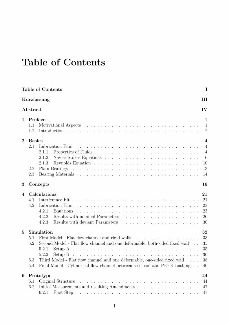
Table of Contents

Table of Contents I

Kurzfassung III

Abstract IV

1 Preface 11.1 Motivational Aspects . . . . . . . . . . . . . . . . . . . . . . . . . . . . . . . . . 11.2 Introduction . . . . . . . . . . . . . . . . . . . . . . . . . . . . . . . . . . . . . . 2

2 Basics 42.1 Lubrication Film . . . . . . . . . . . . . . . . . . . . . . . . . . . . . . . . . . . 4

2.1.1 Properties of Fluids . . . . . . . . . . . . . . . . . . . . . . . . . . . . . . 42.1.2 Navier-Stokes Equations . . . . . . . . . . . . . . . . . . . . . . . . . . . 62.1.3 Reynolds Equation . . . . . . . . . . . . . . . . . . . . . . . . . . . . . . 10

2.2 Plain Bearings . . . . . . . . . . . . . . . . . . . . . . . . . . . . . . . . . . . . . 132.3 Bearing Materials . . . . . . . . . . . . . . . . . . . . . . . . . . . . . . . . . . . 14

3 Concepts 16

4 Calculations 214.1 Interference Fit . . . . . . . . . . . . . . . . . . . . . . . . . . . . . . . . . . . . 214.2 Lubrication Film . . . . . . . . . . . . . . . . . . . . . . . . . . . . . . . . . . . 23

4.2.1 Equations . . . . . . . . . . . . . . . . . . . . . . . . . . . . . . . . . . . 234.2.2 Results with nominal Parameters . . . . . . . . . . . . . . . . . . . . . . 264.2.3 Results with deviant Parameters . . . . . . . . . . . . . . . . . . . . . . 30

5 Simulation 325.1 First Model - Flat flow channel and rigid walls . . . . . . . . . . . . . . . . . . . 335.2 Second Model - Flat flow channel and one deformable, both-sided fixed wall . . 35

5.2.1 Setup A . . . . . . . . . . . . . . . . . . . . . . . . . . . . . . . . . . . . 355.2.2 Setup B . . . . . . . . . . . . . . . . . . . . . . . . . . . . . . . . . . . . 36

5.3 Third Model - Flat flow channel and one deformable, one-sided fixed wall . . . . 385.4 Final Model - Cylindrical flow channel between steel rod and PEEK bushing . . 40

6 Prototype 446.1 Original Structure . . . . . . . . . . . . . . . . . . . . . . . . . . . . . . . . . . . 446.2 Initial Measurements and resulting Amendments . . . . . . . . . . . . . . . . . . 47

6.2.1 First Step . . . . . . . . . . . . . . . . . . . . . . . . . . . . . . . . . . . 47

I

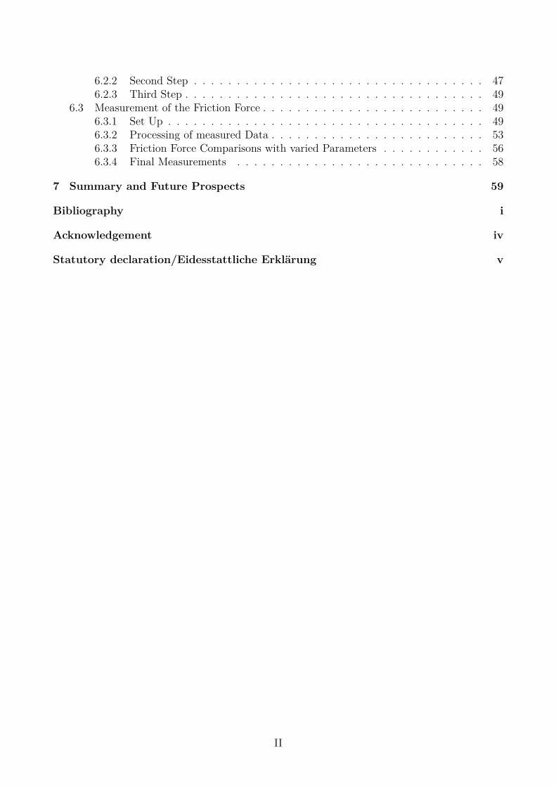
6.2.2 Second Step . . . . . . . . . . . . . . . . . . . . . . . . . . . . . . . . . . 476.2.3 Third Step . . . . . . . . . . . . . . . . . . . . . . . . . . . . . . . . . . . 49

6.3 Measurement of the Friction Force . . . . . . . . . . . . . . . . . . . . . . . . . . 496.3.1 Set Up . . . . . . . . . . . . . . . . . . . . . . . . . . . . . . . . . . . . . 496.3.2 Processing of measured Data . . . . . . . . . . . . . . . . . . . . . . . . . 536.3.3 Friction Force Comparisons with varied Parameters . . . . . . . . . . . . 566.3.4 Final Measurements . . . . . . . . . . . . . . . . . . . . . . . . . . . . . 58

7 Summary and Future Prospects 59

Bibliography i

Acknowledgement iv

Statutory declaration/Eidesstattliche Erklarung v

II

Kurzfassung

Ziel der Masterarbeit war, einen Servozylinder, also Kolben mit Kolbenstange, mittels Druck-versorgung nicht nur eine lineare Hubbewegung machen zu lassen, sondern diese Druckver-sorgung auch zur Lagerung zu verwenden. Fur diese Lagerung soll ein elastohydrostatischesKeilspaltlager sorgen. Fur die ruckstellende Lagerkraft sind Lange und Durchmesser des La-gers, Konizitat, kinematische Viskositat der Flussigkeit im Schmierspalt und Bewegung derKolbenstange in axialer Richtung entscheidend.

In konventionellen Keilspaltlagern wird die keilformige Spaltgeometrie erzielt, indem ein ko-nischer Außen- oder Innenteil gefertigt wird. Dieser Konus sorgt in Verbindung mit einerAuslenkung fur unterschiedliche Druckverlaufe, auf der Seite in welche ausgelenkt wird und derihr gegenuberliegenden Seite. Dadurch ergibt sich eine ruckstellende Wirkung auf Kolbenstangeund Kolben. Im Grenzfall, wo Innen- und Außenteil sich beruhren, ergibt sich so die maximaleRuckstellkraft.

Die Idee zur Adaptierung dieses Lagers besteht darin, sich den hydrostatischen Druck nichtnur fur die Ruckstellkraft zunutze zu machen, sondern auch eine im Allgemeinen nichtkege-lige Aufweitung des Außenteils zu erreichen, um mittels oben beschriebenem ZusammenhangRuckstellkrafte zu erzeugen. Innen- und Außenteil konnen so zylindrisch gefertigt werden. ZurErzielung der notigen Lagerkraft ist ein geeigneter Werkstoff mit passender Dimensionierungfur die Lagerhulse auszuwahlen, der die notige Aufweitung erreicht.

Die Hubbewegung von Kolben und Stange soll fur ein Laborexperiment dienen, bei dem dieStirnflache der Stange in einem Rohr einen definierten und bewegbaren Abschluss bildet. Die-ser bewegte Abschluss stellt eine Randbedingung mit bekannter Geschwindigkeit dar. DieStromungsgeschwindigkeit an der Begrenzungsflache ist gleich der Geschwindigkeit der Kolben-stange, welche einfach gemessen werden kann. Fur eine moglichst dynamische Bewegung ist esnotig, Kolben und Stange moglichst reibungsarm zu lagern, und der Leckstrom Richtung Rohrsollte moglichst klein sein, um einen Einfluss auf die Rohrstromung zu vermeiden.

Aufgabenstellung:

• Literaturrecherche und Erstellung diverser Konzepte

• Simulation der (nichtkegeligen) Aufweitung und der Lagerkraft

• Berechnungen an vereinfachten Modellen zur Evaluierung der Simulationsdaten

• Aufbau und Inbetriebnahme

• Messungen

• Dokumentation

III

Abstract

The goal of this master thesis was the development of a servo cylinder, that uses the pressuresupply not only for moving the piston and the piston rod forward and backward, but also fortwo hydrostatic linear bearings. The restoring bearing force depends on length and diameter ofthe bearing, conicity, kinematic viscosity of the fluid inside the lubrication gap and a possiblevelocity of the cylinder in axial direction.

In conventional bearings a wedge-shaped lubrication gap is a result of a conical bushing or rod.This conus and a displacement of the rod in radial direction causes different pressure curves onthe two opposite sides. The first is the side in the direction of the displacement and the secondis opposing to the first. Resulting forces acting on the cylinder are the outcome of this differentpressure curves and move the piston and the piston rod back to the center. If the rod touchesthe bushing, the restoring force reaches its maximum.

The idea of an adjustment is to use the pressure supply also to achieve a deformation ofthe bushing and provoke the restoring force. The deformation is a nonlinear widening. Soa restoring force results from pressure supply and widening. The rod and the bushings canbe produced cylindrically and don’t have to be manufactured conically. A material and thedimensions have to be selected, to accomplish the right widening of the bushings.

The linear movement of the piston and its rod is important for a laboratory experiment. Theend face of one piston rod should be used as a “moveable boundary condition” of a pipe. Thevelocity of the boundary is easy to determine by measuring the velocity of the piston rod.So flow experiments can be done, which can be compared with simulations. It is importantthat the friction and the leakage flow between piston and rod and its outer parts is as low asreasonably achievable.

Assignment of tasks:

• Review of literature and creating varying concepts

• Simulation of the non tapered widening and restoring force

• Calculations of simplified models to evaluate the simulation data

• Assembling and commissioning

• Measurements

• Documentation

IV

Chapter 1

Preface

1.1 Motivational Aspects“Wissenschaftler(innen) sind Abenteurer(innen) an der Grenze des Wissens. Im

Gegensatz zu den großen Entdeckern der Welt wie Vasco da Gama, Fernando de Ma-gellan, Alexander von Humboldt und Jacques Piccard bewegen sie sich jedoch nichtin der physischen Welt, sondern im Geiste. Sie erweitern das Wissen an dessenGrenze, jener zwischen Nichtwissen und Wissen. Diese Grenze hat die Eigenschaftsich auszudehnen, da mit Antworten, also Entdeckungen und Erfindungen, auchautomatisch immer neue Fragen, also mogliche Wege ins Unbekannte, aufgezeigtwerden.” [1]

This text passage is a statement of Gerda Buchberger an Upper Austrian scientist and is partof her master thesis about concepts of flexible touchpads.

So many scientists, researchers and academics try to expand the boundaries of human know-ledge. Everyday young scientists, experienced engineers and scholarly persons explore theore-tical physics, molecular biology, meteorology, chemistry, mechanics, semiconductor technologyor another specialist field of natural science or technology.In former times highly educated people often lived on the margins of society. Nowadays eve-rything revolves around advancement, especially the engineering progress. Electronic systemshave to be smaller with less power consumption, mechanical structures have to weigh less andhydraulics has to be more efficient. And engineers and scientists have to ensure that.

Hydraulic engineers have to evolve new hydraulic components and research new theoreticalrelationships. Based on the model of Blaise Pascal, Joseph Bramah or William George Arm-strong down to the present day, engineers develop new hydraulic valves, gear pumps, hydraulicaccumulators or study new aspects of fluid mechanics. [2]Today we now, even in Ancient Greek various apparats and machineries with fluid power wereknown and also used. Maybe the most famous greek engineer was Heron of Alexandria. Heinvented a vending machine, a force pump and a reaction engine that works like a rocket engine.Therefore it is not surprising that, “Hydraulics” originates from the Ancient Greek words Õdwrhydor “water” and aÔlìc aulos “pipe”. [2] [3]

Lubrication of moving parts was always an important issue. Without lubrication the friction isvery high and parts get broken by mechanical or thermal wear. So lubrication and hydraulics

1

go hand in hand. Nowadays the high performance of hydraulics, needs exact knowlegde offriction to avoid undesired effects.

1.2 IntroductionIt is difficult to apply analytical models of complicated geometries of fluid power components.So Computational Fluid Dynamics (CFD) is a possible way to determine the velocity andthe pressure field. The full 3D resolution is not always needed and in consideration of thevery long calculating time of the two (3D) fields with small grid size and the related highcosts, simpler models are often sufficient. One of these methods is to combine transmissionline models with quasi-steady friction for cylindrical parts with CFD models for geometrieswith more complexity. Such a combination of these two models was published by Fries andManhartsgruber in 2013 and was used by them in 2014. [4] [5]

The test rig of the experiments in 2014 is made out of aluminum cubes with drillings to realizethe flow channel. The cubes provide a high wall thickness, to reduce the flexibilty of the walland to avoid an increase of the hydraulic capacity. Pressure sensors are attached to everysecond cube. The fluid has to pass a servo directional valve from Bosch Rexroth AG type4WS2EM6-2X/25B11ET315K17EV with a nominal flow of 25 l/min, an inlet pressure rangefrom 10 to 315 bar and a spool overlap of 0 to 0.5%. To leave the test rig, the fluid has to passa throttle after the last cube. The flow channel is cylindric and L-shaped. The rig is shown inFigure 1.1. [5]

The inlet flow profile is determined by the geometry of the servo directional valve. This shouldbe changed. The flow should be caused by a rod that moves in a flow channel, like pointed inFigure 1.2. So the boundary condition of the lateral face of the fluid can be described easily.The position, the velocity and the acceleration of the lateral face of the fluid are described bythe motion of the piston rod.

Thus to replace the servo directional valve by a piston rod, leads to easy and well-definedboundary conditions at the linear actuator. Otherwise the conditions depend on the position ofthe servo valve spool and on the pressure in a quite complicated way. With the new advancedtest rig the simulation results are better comparable with experimental measurements. To movethe piston rod and to reduce friction and wear, different applications are possible.

Drive options:

• Servo cylinder: A piston and the piston rod moves back and forth in a pipe. The motionof the cylinder can be set by a closed loop controller. For example the motion is sinusoidalor rectangular. The cylinder gets the power from pressurized hydraulic oil and is actuatedby a servo valve.

• Drop hammer: The piston gets the power from a known mass, dropped from a knownheight to impact the piston. It leads to a shock load.

Bearing options:

• Plain bearings (including fluid bearings)

• Bearings with rolling elements

2

(a) Picture (b) Scheme

Figure 1.1: Picture and scheme of the test rig used by [5].

• Magnetic bearings

The first step is the design of the different options and selection of the best one. To choosethe right one, the advantages and disadvantages have to be determined. Then the calculationsand simulations are required to devise a first prefiguration and, where necessary, to introduceenhancements. With an efficient installation, new experiments - to compare them with CFDsimulations - can be done.

Figure 1.2: Piston rod moves in flow channel

3

Chapter 2

Basics

2.1 Lubrication Film

2.1.1 Properties of FluidsFluids are substances without a definite shape that deform continuously under an applied shearstress, so they cannot resist tangential forces and involve three out of four state of matters.Fluids involve liquid and gaseous phase and plasma. The material consists of a lot of atoms andmolecules. So any substance is discontinuous in a microscopic examination. But for macroscopicconsideration it is better to examine it as a continuous material. [6]

Density

The density ρ of a substance is defined as mass per unit volume:

ρ = mass

unit volume= m

V(2.1)

But it also depends on the temperature T and absolut pressure p. There are two linear modelsfor the dependencies of the density of liquids and only one equation for gases.

Normally the thermal expansion is positive with the exception of some special cases. Forexample liquid water below 4 ◦C. The formula of the first relation:

ρ = ρ0

1− γ ∆ϑ (2.2)

ρ0 represents the reference density at reference temperature. ∆ϑ means the difference betweenactual temperature and reference temperature und γ denotes the volumetric thermal expansioncoefficient and is defined as γ = 1

V∂V∂ϑ

. [7]

For liquids there is also a similar connection between the change of pressure p and density ρ:

ρ = ρ0

1− β ∆p (2.3)

ρ0 represents the reference density by reference pressure. ∆p means the difference betweenactual pressure and reference pressure und β denotes the compressibility and is defined asβ = − 1

V∂V∂p

. [7] [8]

4

In the other case (for gases) a different relation exists and is described by the ideal gas law.There is only one formula needed:

ρ = p

Rs T(2.4)

p means the absolut pressure. The variable T represents the absolut temperature and Rs isthe specific gas constant. For closer description more information about the thermodynamicprocess is needed. The process can be isothermal, adiabatic, isobaric, isochoric or there is noideal process. [6] [7]

Furthermore the equation of state of ideal gases is no longer required, because this thesis isengaged in lubrication by oils.

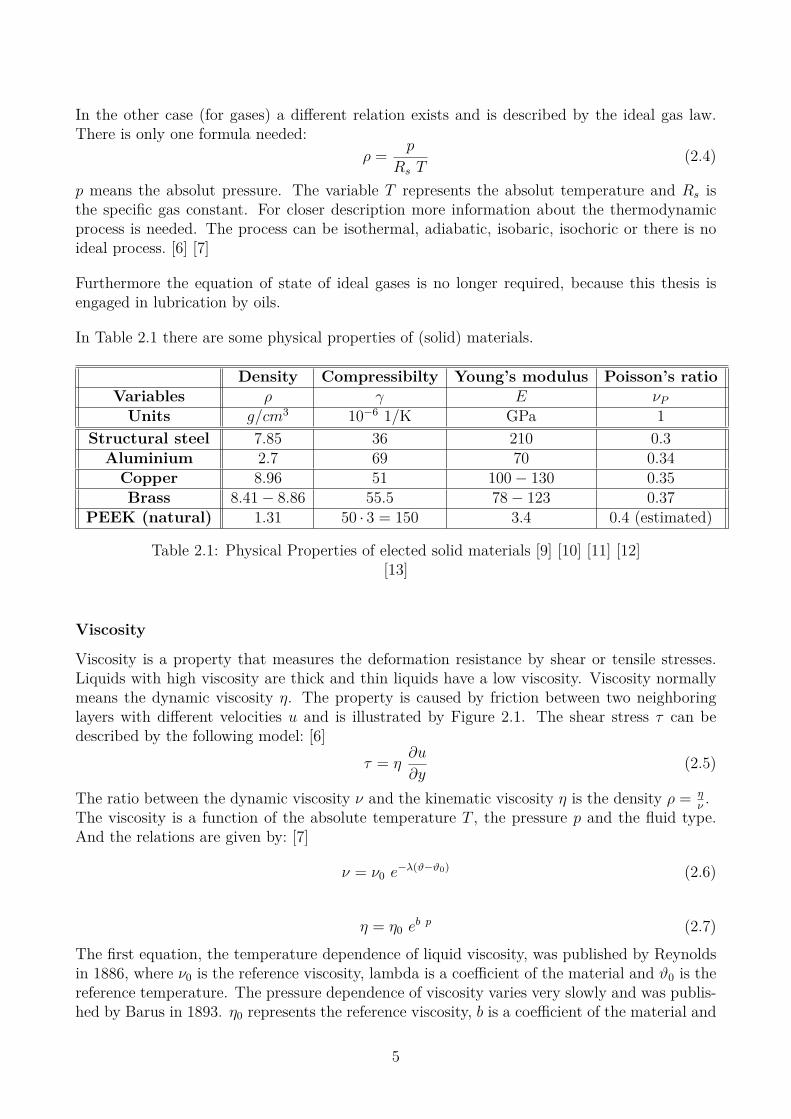
In Table 2.1 there are some physical properties of (solid) materials.

Density Compressibilty Young’s modulus Poisson’s ratioVariables ρ γ E νP

Units g/cm3 10−6 1/K GPa 1Structural steel 7.85 36 210 0.3

Aluminium 2.7 69 70 0.34Copper 8.96 51 100− 130 0.35Brass 8.41− 8.86 55.5 78− 123 0.37

PEEK (natural) 1.31 50 · 3 = 150 3.4 0.4 (estimated)

Table 2.1: Physical Properties of elected solid materials [9] [10] [11] [12][13]

Viscosity

Viscosity is a property that measures the deformation resistance by shear or tensile stresses.Liquids with high viscosity are thick and thin liquids have a low viscosity. Viscosity normallymeans the dynamic viscosity η. The property is caused by friction between two neighboringlayers with different velocities u and is illustrated by Figure 2.1. The shear stress τ can bedescribed by the following model: [6]

τ = η∂u

∂y(2.5)

The ratio between the dynamic viscosity ν and the kinematic viscosity η is the density ρ = ην.

The viscosity is a function of the absolute temperature T , the pressure p and the fluid type.And the relations are given by: [7]

ν = ν0 e−λ(ϑ−ϑ0) (2.6)

η = η0 eb p (2.7)

The first equation, the temperature dependence of liquid viscosity, was published by Reynoldsin 1886, where ν0 is the reference viscosity, lambda is a coefficient of the material and ϑ0 is thereference temperature. The pressure dependence of viscosity varies very slowly and was publis-hed by Barus in 1893. η0 represents the reference viscosity, b is a coefficient of the material and

5

Figure 2.1: Shear of fluid between plates. Friction causes this curve of shear.

p denotes the pressure. [6] [7] [14] [15] [16]

Effects of temperature and pressure on the viscosity of gases are different from the effects onthe viscosity of liquids.

The commonly used hydraulic oils HLP 32 and HLP 46 have kinematic viscosities of around32 mm2/s respectively 46 mm2/s and viscosity indices of 192 respectively 187. The densitiesare 911 kg/m3 and 921 kg/m3. [17]The volumetric thermal expansion coefficient γ is 6.5 · 10−4 − 7.5 · 10−4 1/K and the compres-sibility β 1.4− 1.6 GPa. [8]

2.1.2 Navier-Stokes EquationsThe Navier-Stokes equations are a set of partial differential equations. The fundamental con-servation laws are valid, if the fluid can be seen as a continuous medium. There are a numberof constitutive equations based on the balance of mass and momentum.

The following equations are based on [18] and [19] and the Einstein notation is used. First ofall the material derivative D

Dtis introduced, where vi represents a component of the velocity

vector, xi is the i-th spatial coordinate and t means time:

D

Dt= ∂

∂t+ vi

∂

∂xi(2.8)

There are two different descriptions of motion and derivatives. The material derivative is withrespect to a moving particle and the Eularian derivative is a derivation at a fixed point. Thefirst term on the right side is the Eulerian derivative, a partial derivative with respect to thetime. The second one is called convective derivative and is caused by following the trajectoryof a particle. [6] [18]

The mass continuity equation says, that the mass of volume of fluid δm = ρ δV does not changein time. There are no sources or sinks of mass inside. The volume has to be big enough thatBrownian motion has not to be considered:

d(δm)dt

= d

dt(ρ δV ) = δV

dρ

dt+ ρ

d(δV )dt

= 0 (2.9)

6

For the derivation of density the material derivative has to be used and by using the divergenceof velocity ∂vi

∂xi= 1

δV∂(δV )∂t

:

d(δm)dt

= δV

(∂ρ

∂t+ vi

∂ρ

∂xi

)+ ρ δV

∂vi∂xi

= ∂ρ

∂t+ vi

∂ρ

∂xi+ ρ

∂vi∂xi

= 0 (2.10)

In case of an incompressible fluid (ρ = constant) the equation reduces to:

∂vi∂xi

= 0 (2.11)

In this case the divergence of velocity is zero. [6] [18] [20]

Momentum continuity means variation in time of the momentum of a volume of fluid I is equalto the acting forces:

dIjdt

= d(m vj)dt

= ρ δVDvjDt

= FDj + FEj + d(δIM)jdt

(2.12)

FDj represents a component of the force caused by pressure difference as shown in Figure 2.2.The forces can be calculated by the balance of forces on a small cubic element. The pressuredifference between two sides multiplied by the area equals to FDj.FEj means a component of the force applied by a remote action such as gravitational, magneticor electrical forces. fEj represents FEj per unit mass.And d(δIM )j

dtdenotes the molecular-dependent momentum input per unit time. It depends on the

j momentum transported in the direction i per unit area and unit time as shown in Figure 2.3.

Figure 2.2: Considerations concerning pressure on a fluid element

Arising from the balance of forces and use of Taylor series:

FDj = p(xj)|δAj| − p(xj + δxj)|δAj| = −∂p

∂xjδV (2.13)

d(δIM)jdt

= −τij(xi)|δAi|+ τij(xi + δxi)|δAi| =∂τij∂xj

δV (2.14)

7

Figure 2.3: Molecular-dependent momentum input

τij is the component j of the stress acting of the fluid element perpendicular to the axis i. NowEquation 2.12 can be expressed by:

DvjDt

= −1ρ

∂p

∂xj+ fEj + 1

ρ

∂τij∂xj

(2.15)

To determine the different contributions to τij caused by the total momentum transport, theconsiderations below are recommended.The relations for the first term are shown in Figure 2.4. There are six directions. A sixth ofthe molecules move in positive xi direction. The number of molecules zi moving in xi directionand passing plane δAi in time ∆t is:

zi = 16 vth nm δAi ∆t (2.16)

Figure 2.4: Momentum due to flow through the plane

δAi is oriented in the i direction. vth is the mean velocity of the molecules in direction i, n isthe number of molecules per unit volume. The difference of momentum over δAi in positive

8

and negative i direction:

∆i+ij = 16 vth nm mm (vj(xi + l)− vj(xi)) δAi ∆t ≈ 1

6 vth nm mm l∂vj∂xi

δAi ∆t (2.17)

∆i−ij = −16 vth nm mm (vj(xi − l)− vj(xi)) δAi ∆t ≈ 1

6 vth nm mm l∂vj∂xi

δAi ∆t (2.18)

The length l means a distance which describes the “starting point” of the molecules above orbelow the plane. The net momentum can be expressed by:

τ Iij =∆i+ij + ∆i−ijδAi ∆t = 1

3 vth ρ l∂vj∂xi

(2.19)

The second term can be explained by using Figure 2.5. A sixth of the molecules move throughthe plain B1i and make a fluctuation movement in j direction and impacts on δAi, with ananalog explanation for B2i:

∆i+ij = 16 vth nm mm (vi(xj − l)− vi(xj)) δAi ∆t ≈ −1

6 vth nm mm l∂vi∂xj

δAi ∆t (2.20)

∆i−ij = −16 vth nm mm (vi(xj + l)− vi(xj)) δAi ∆t ≈ −1

6 vth nm mm l∂vi∂xj

δAi ∆t (2.21)

Figure 2.5: Momentum caused by molecular motion with mean velocity

The net momentum of the second contribution:

τ IIij = −∆i+ij + ∆i−ijδAi ∆t = 1

3 vth ρ l∂ui∂xj

(2.22)

In case of incompressible fluids τij consists of two terms. In case of a compressible fluid thechange of volume has to be considered:

τ′

ij = −23 η δij

∂vk∂vk

(2.23)

The result τij can be written in terms of an arbitrary coordinate system:

τij = τ Iij + τ IIij + τ′

ij = 13 vth ρ l

(∂vj∂xi

+ ∂vi∂xj

)− 2

3 η δij∂vk∂xk

(2.24)

9

In generally the components ∂vj

∂xiand ∂vi

∂xjare not zero. The viscosity η is equal to 1

3 vth ρ l.A special case would be a Couette flow, shown in Figure 2.1. It is a laminar flow between astationary plate and a moving plate. Only one of the three velocity components is not zero.

The Cartesian Navier-Stokes equations of compressible Newtonian fluids consist of mass conti-nuity equation and the system of equations regarding to conservation of momentum:

∂ρ

∂t+ ∂(ρvi)

∂xi= 0 (2.25)

ρ∂vi∂t

+ ρ vj∂vi∂xj

= ρ fEi −∂p

∂xi+ ∂

∂xj

(η

(∂vi∂xj

+ ∂vj∂xi− 2

3 δij∂vk∂xk

))(2.26)

δij is representing the Kronecker delta.

Formulation if the Newtonian fluids are incompressible:

∂vi∂xi

= 0 (2.27)

∂vi∂t

+ vj∂vi∂xj

= fEi −1ρ

∂p

∂xi+ ν

∂2vi∂xj2 (2.28)

2.1.3 Reynolds EquationOsborne Reynolds published an important paper in 1886. It was the hour of birth of thetheory of lubrication. Reynolds defined lubrication as “action of oils and other viscous fluidsto diminish friction and wear between solid surfaces”. [15]

The following derivation of the Reynolds equation is based on [21] and [22]. The Reynoldsequation is a differential equation. It is governing the pressure distribution of thin fluid films.The thickness of the film h is in z direction and b is the width in y direction and the motion isin x direction.The Einstein summation convention is not longer used. Instead of x1, x2 and x3 we use x, yand z. u1, u2 and u3 are replaced by u, v and w. These are the fluid velocities in x, y and zdirection.The forces acting on the surfaces of a voxel are shown in Figure 2.6.

Figure 2.6: Forces on the surfaces of a voxel.

10

The balance of forces can be expressed as:(p+ ∂p

∂xdx

)dz − p dz −

(τ + ∂τ

∂zdz

)dx+ τ dx = 0 (2.29)

Reduction leads to:∂p

∂x= ∂τ

∂z(2.30)

With insertion of Equation 2.5, the equations in 3 dimensions are:

∂p

∂x= ∂

∂z

(η∂u

∂z

)(2.31)

∂p

∂y= ∂

∂z

(η∂v

∂z

)(2.32)

∂p

∂z= 0 (2.33)

The integration of the upper equations leads to:

∂u

∂z= z

η

∂p

∂x+ A1

η(2.34)

∂v

∂z= z

η

∂p

∂y+ B1

η(2.35)

η represents the averaged value of the dynamic viscosity and Ai and Bi are integration constants.Another integration gives the velocities as:

u = z2

2 η∂p

∂x+ z

ηA1 + A2 (2.36)

v = z2

2 η∂p

∂y+ z

ηB1 +B2 (2.37)

The boundary values of the velocities are u(z = 0) = ub, v(z = 0) = vb, u(z = h) = ua andv(z = h) = va, if no slip is assumed. With boundary conditions Equations 2.36 and 2.37 turninto:

u = −z(h− z2 η

)∂p

∂x+(

1− z

h

)ub + z

hua (2.38)

v = −z(h− z2 η

)∂p

∂y+(

1− z

h

)vb + z

hva (2.39)

The volume flow rates per unit width in the two directions of x and y are:

Vx =∫ h

0u dz = − h3

12 η∂p

∂x+ h (ua + ub)

2 (2.40)

Vy =∫ h

0u dz = − h3

12 η∂p

∂y+ h (va + vb)

2 (2.41)

Equation 2.25 in new notation:

∂ρ

∂t+ ∂(ρu)

∂x+ ∂(ρv)

∂y+ ∂(ρw)

∂z= 0 (2.42)

11

The dynamic viscosity η and the density ρ are functions of x and y. A common rule of integra-tion: ∫ h

0

∂

∂x[f(x, y, z)] dz = −f(x, y, z) ∂h

∂x+ ∂

∂x

[∫ h

0f(x, y, z) dz

](2.43)

With Equation 2.43 the Equation 2.42 in integral form can be splitted:∫ h

0

∂(ρu)∂x

= −ρ ua∂h

∂x+ ∂

∂x

(ρ∫ h

0u dz

)(2.44)

∫ h

0

∂(ρv)∂y

= −ρ va∂h

∂y+ ∂

∂y

(ρ∫ h

0v dz

)(2.45)

∫ h

0

∂(ρw)∂z

= ρ (wa − wb) (2.46)

Introducing this three integrals into Equation 2.42, the integral form provides:

h∂ρ

∂t− ρ ua

∂h

∂x+ ∂

∂x

(ρ∫ h

0u dz

)− ρ va

∂h

∂y+ ∂

∂y

(ρ∫ h

0v dz

)+ ρ (wa − wb) = 0 (2.47)

Substituting the flow rate expressions into the last Equation:

h∂ρ

∂t− ρ ua

∂h

∂x− ρ va

∂h

∂y+ ρ (wa − wb)−

∂

∂x

(ρ h3

12 η∂p

∂x

)+ ∂

∂x

ρ h (ua + ub)2 − ∂

∂y

(ρ h3

12 η∂p

∂y

)+ ∂

∂x

ρ h (va + vb)2 = 0 (2.48)

The first term is the local expansion term and describes the net flow rate. The second to fourthterms are also net flow rates caused by a squeezing motion. The fifth and seventh term arePoiseuille terms provoked by pressure gradient. And the sixth and eighth term are Couetteterms caused by velocities of the solid bodies.

This equation is a generalized form of the Reynolds equation but it is quite complicated. Theexpression of journal bearings can be reduced with subsequent assumptions:

ρ = constant η = constant (2.49)ua = U ub = 0 (2.50)va = 0 vb = 0 (2.51)wa = 0 wb = 0 (2.52)

And the bodies are rigid.

A cross section of a journal bearing is shown in Figure 2.7. There is a linear motion of thebushing in axial direction. The cylindric form is rolled out and the film thickness h is a functionof x and y. The rod is eccentric but not tilted.If there is no motion in y direction and with the above assumptions, the Reynolds equation canbe rearranged:

∂

∂x

(h3 ∂p

∂x

)+ ∂

∂y

(h3 ∂p

∂y

)= 6 η U ∂h

∂x(2.53)

12

Figure 2.7: Slide bearing

The equation can be converted to polar coordinates. ∂∂x

is not changed. ∂∂y

turns into 1rb

∂∂φ

,where rb means the radius and φ the angular coordinate. The Equation 2.53 in polar coordi-nates:

∂

∂x

(h3 ∂p

∂x

)+ 1rb

∂

∂φ

(h3

rb

∂p

∂φ

)= ∂

∂x

(h3 ∂p

∂x

)+ 1r2b

∂

∂φ

(h3 ∂p

∂φ

)= 6 η U ∂h

∂x(2.54)

With knowledge of h = h(x, φ), η, U and rb the pressure distribution is definable.

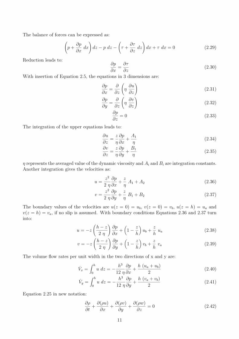
2.2 Plain BearingsBearings allow relative motion between two parts and does not permit motion in the directionof the loads. Bearings are necessary to avoid or reduce adhesive, corrosive, abrasive, erosiveand fatigue wear, corrosion and yielding. Friction should be reduced and should be as lowas reasonably achievable. There are two common types of bearings: Slide/plain bearings andbearings with rolling elements. Bearings with rolling elements will not be discussed. There area number of advantages of slide bearings over rolling element bearings: Simple design, smallradial space, quiet, not sensitive to dust, high load capacity, high rotational speeds achievable,easy to replace and other reasons. [23]

The concepts of lubrication of a plain bearing comprise: Bearing materials that are the lubri-cant. They do not need a lubricant from an external source. Bearings with walls that containthe lubricant and bearings which need the lubricant from an external source like oil. [24]

There are different lubrication concepts of fluid bearings. On the one hand there are hydrostaticbearings with externally pressurized lubrication. In this case no relative motion is needed toseparate the surfaces. On the other hand the hydrodynamic bearings need a relative motionof the solid bodies to press fluid into the wedge-shaped zone. A special form of hydrodynamicbearings are elastohydrodynamic bearings, where the deformation of the solid bodies cannot beneglected. Further the boundary lubrication is the fourth concept of lubrication. The conceptscan be used for radial or axial bearings. [23]

Another distinction of plain bearings can be made between integral bearings, bushings and

13

two-piece bearings. An integral bearing is a hole in a component and the surface of the holeis one of the bearing surfaces. The bushing is inserted into a casing to create a bearing. It iseasier to replace the bushing than the whole component, so bushings are more common thanintegral bearings. The two-piece bearings have two shells, which form the bearing housing. Theshells are also easy to replace. [24]

To avoid high friction at the beginning of a motion and in cases with low motion a hydrosta-tic fluid bearing is to be preferred. The pressure supply makes sure that there is no contactbetween the two surfaces, as long as the supply is well.

2.3 Bearing MaterialsThere are various requirements of bearings and so the choice of the correct combination ofmaterials is essential for the proper functioning. Some important properties of bearing materi-als: [23] [25] [26]

• Fatigue strength: The maximum value of cyclic stress that can be applied. The materialhas to withstand an infinite number of cycles.

• Wear resistance: The resistance of the material against erosion caused by particles andthe direct contact between two solid bodies.

• Seizure resistance: Resistance against friction welding.

• Conformability: The possibility to adjust misalignments of the geometries.

• Embeddability: The ability to “allow” particles between the surfaces without higherwear.

• Corrosion resistance: Corrosion means the oxidation of an element with Oxygen - anchemical reaction.

• Cavitation resistance: Small imploding bubbles cause impact stress.

• Thermal conductivity: The property of a material to conduct the (friction induced)heat.

The above list with properties defines the materials, which can be used. The surface of thejournal should be three to five times as hard as the surface of the bearing and is mostly madeout of steel. The Rockwell hardness should be above 50 HRC and a surface that is as smoothas possible. The surface should be fine grinded and lapped. Another possibility to enhanceseveral properties is a treatment of the surface. [26]

There are much more bearing than journal materials. The used material depends on the specificrequirement profile and the type of lubrication. Here are some relevant bearing materials: [25][26]

• Steel: Cast iron and cased-harden or nitrated steel are used.

• Tin: Tin in conjunction with lead, copper or antimony has excellent friction characteri-stics, but it needs a supporting body because of the softness.

14

• Zinc: Zinc in alloys with aluminium and copper has also good friction characteristicsand is a very cheap material.

• Lead: Lead in combination with copper, tin, zinc or bismuth is very ductile. It is oftenused for big bearings and it is nonsensitive to disturbances of the lubrication. Lead shouldbe avoid as construction material, because it is poisonous.

• Copper: It is used in various copper alloys and is the most commonly used bearingmaterial. It has a high tensile strength and high heat conductivity. The embeddability islow.

• Aluminium: Aluminium with copper, steel, zinc, manganese, silicon or tin is used inbearings of light alloy housings. So the thermal expansion of bearing and housing areequal.

• Plastics: Thermoplastic resins (polyamides (PA), polyethylene (PE) or polytetrafluo-roethylene (PTFE)) can be used on their own and in combination with other materials.Thermosetting resins have high friction coefficients and need PTFE or graphite fittings. Incase of low velocities bearings made out of plastic are better suitable than metal bearings.But the creep and the thermal expansion are higher.

• Ceramics: Ceramics are very hard materials and they are used in pumps hoisting cor-rosive substances. Ceramic bearings are usable up to 2000 bar and 1700 ◦C.

15

Chapter 3

Concepts

In Chapter 1.1 drive and bearing options are mentioned. The drop hammer method leads toa shock load and the use of a servo cylinder to a continuous load. This results in the selectionof the servo cylinder, because the test rig should be used with a continuous input. The choiceof the right bearing is more complicated. Friction can be categorized into solid/boundaryfriction, mixed friction and fluid friction and is described by the Stribeck curve. There is aminimum value between the fully developed fluid film lubrication and the solid interactions.To avoid Coulomb friction, which is named after Charles Augustin de Coulomb and means dryfriction, often fluid bearings are used. In Chapter 2.2 hydrostatic fluid bearings are introduced,to prevent higher friction, as result of low motion. The fluid film makes sure that there isno contact between the two surfaces, as long as the pressure supply is well. There are twodifferent hydrostatic bearings. The first one with constant thickness of the lubrication gap andthe second one with variation of the thickness. The two versions of fluid static bearings aredemonstrated in Figure 3.1 and 3.2.

Figure 3.1: Fluid static bearing with constant thickness of the gap. Published in [27].

In Figure 3.1 chambers are supplied with pressurized oil. Between the pressure chambers(called “Lagertasche” in German) and the cylinder chambers and the environment are smallgaps (called “Dichtspalt”) with grooves. The grooves are necessary to remove the leakage oil(called “Leckol”). An eccentricity leads to higher pressure in sections of the pressure chamberswhich are in direction of the deflection and reduces the pressure on the other side. The pressure

16

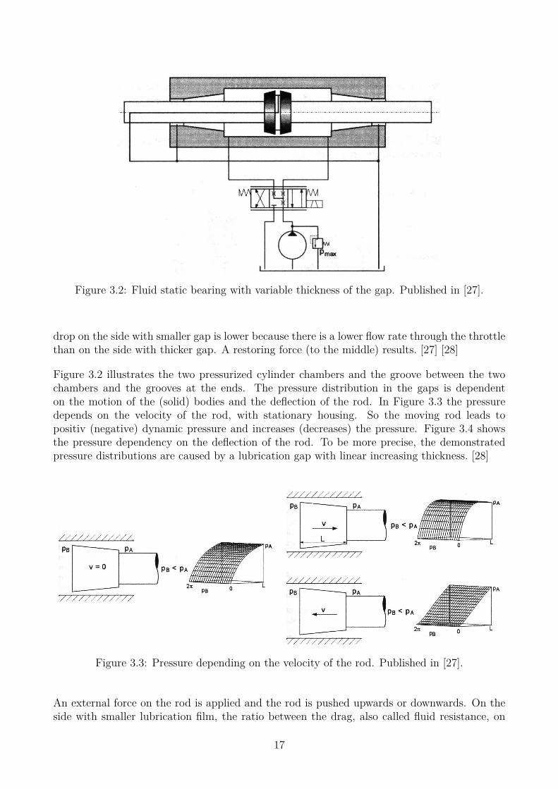
Figure 3.2: Fluid static bearing with variable thickness of the gap. Published in [27].

drop on the side with smaller gap is lower because there is a lower flow rate through the throttlethan on the side with thicker gap. A restoring force (to the middle) results. [27] [28]

Figure 3.2 illustrates the two pressurized cylinder chambers and the groove between the twochambers and the grooves at the ends. The pressure distribution in the gaps is dependenton the motion of the (solid) bodies and the deflection of the rod. In Figure 3.3 the pressuredepends on the velocity of the rod, with stationary housing. So the moving rod leads topositiv (negative) dynamic pressure and increases (decreases) the pressure. Figure 3.4 showsthe pressure dependency on the deflection of the rod. To be more precise, the demonstratedpressure distributions are caused by a lubrication gap with linear increasing thickness. [28]

Figure 3.3: Pressure depending on the velocity of the rod. Published in [27].

An external force on the rod is applied and the rod is pushed upwards or downwards. On theside with smaller lubrication film, the ratio between the drag, also called fluid resistance, on

17

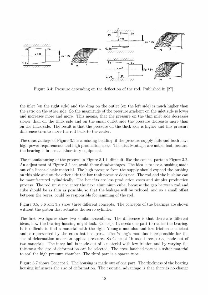
Figure 3.4: Pressure depending on the deflection of the rod. Published in [27].

the inlet (on the right side) and the drag on the outlet (on the left side) is much higher thanthe ratio on the other side. So the magnitude of the pressure gradient on the inlet side is lowerand increases more and more. This means, that the pressure on the thin inlet side decreasesslower than on the thick side and on the small outlet side the pressure decreases more thanon the thick side. The result is that the pressure on the thick side is higher and this pressuredifference tries to move the rod back to the center.

The disadvantage of Figure 3.1 is a missing bedding, if the pressure supply fails and both havehigh power requirements and high production costs. The disadvantages are not so bad, becausethe bearing is in use as laboratory equipment.

The manufacturing of the grooves in Figure 3.1 is difficult, like the conical parts in Figure 3.2.An adjustment of Figure 3.2 can avoid these disadvantages. The idea is to use a bushing madeout of a linear-elastic material. The high pressure from the supply should expand the bushingon this side and on the other side the low tank pressure does not. The rod and the bushing canbe manufactured cylindrically. The benefits are less production costs and simpler productionprocess. The rod must not enter the next aluminium cube, because the gap between rod andcube should be as thin as possible, so that the leakage will be reduced, and so a small offsetbetween the bores, could be responsible for jamming of the rod.

Figure 3.5, 3.6 and 3.7 show three different concepts. The concepts of the bearings are shownwithout the piston that actuates the servo cylinder.

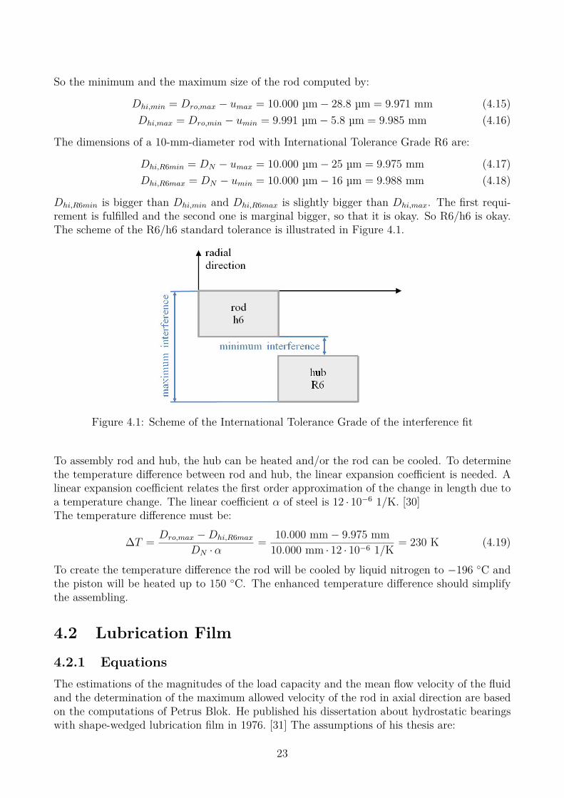
The first two figures show two similar assemblies. The difference is that there are differentideas, how the bearing housing might look. Concept 1a needs one part to realize the bearing.It is difficult to find a material with the right Young’s modulus and low friction coefficientand is represented by the cross hatched part. The Young’s modulus is responsible for thesize of deformation under an applied pressure. So Concept 1b uses three parts, made out oftwo materials. The inner hull is made out of a material with low friction and by varying thethickness the size of deformation can be selected. The cross hatched part is a softer materialto seal the high pressure chamber. The third part is a spacer tube.

Figure 3.7 shows Concept 2. The housing is made out of one part. The thickness of the bearinghousing influences the size of deformation. The essential advantage is that there is no change

18

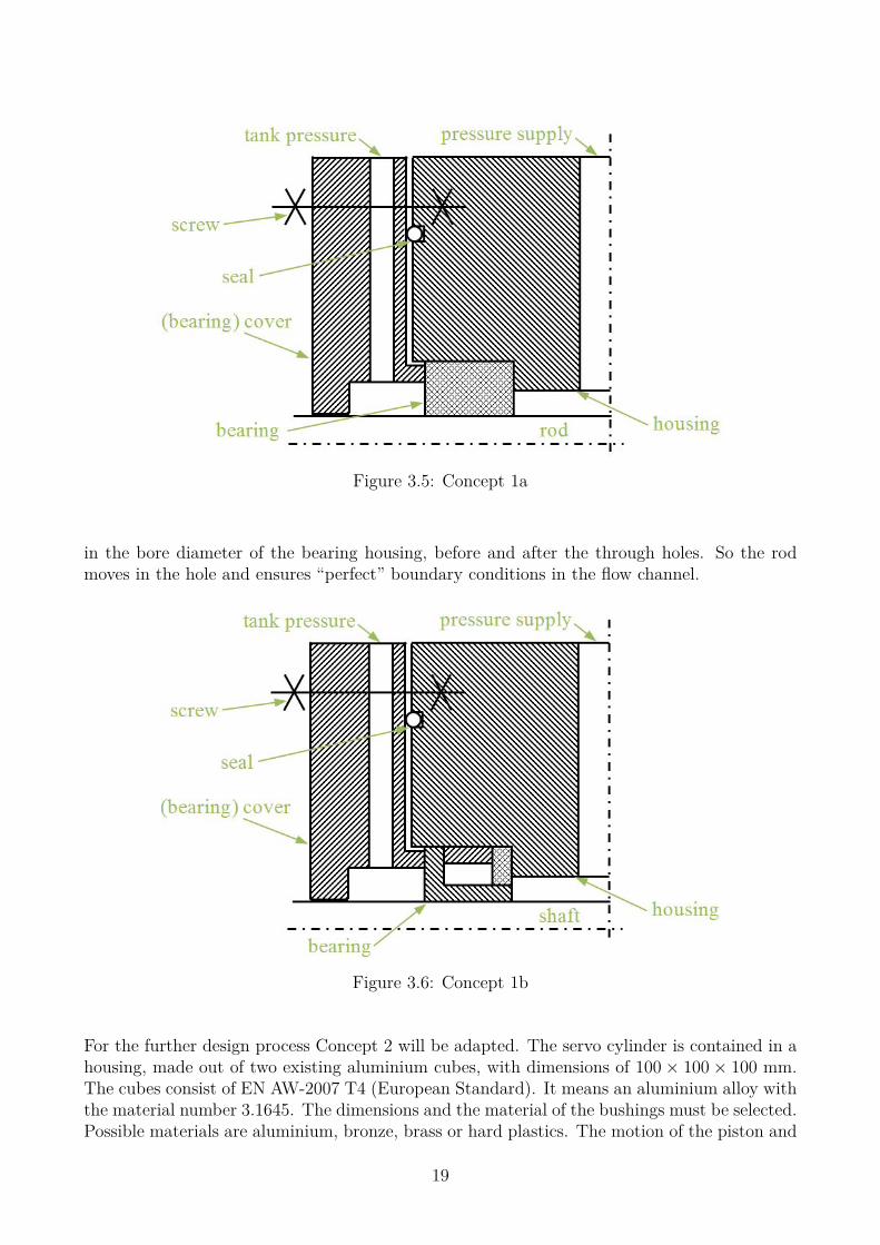
Figure 3.5: Concept 1a

in the bore diameter of the bearing housing, before and after the through holes. So the rodmoves in the hole and ensures “perfect” boundary conditions in the flow channel.

Figure 3.6: Concept 1b

For the further design process Concept 2 will be adapted. The servo cylinder is contained in ahousing, made out of two existing aluminium cubes, with dimensions of 100× 100× 100 mm.The cubes consist of EN AW-2007 T4 (European Standard). It means an aluminium alloy withthe material number 3.1645. The dimensions and the material of the bushings must be selected.Possible materials are aluminium, bronze, brass or hard plastics. The motion of the piston and

19

Figure 3.7: Concept 2

piston rod has to be detected. The servo cylinder will be actuated by the servo directionalvalve from Bosch Rexroth AG type 4WS2EM6-2X/25B11ET315K17EV. The hole pattern ofthe hydraulic connections of the servo directional valve is in according to ISO 4401-03-02-0-05.The diameter of the piston rod is 10 mm and the piston has a diameter of 30 mm. Piston andpiston rod are made out of steel. The properties of the used materials are in Table 2.1.

20

Chapter 4

Calculations

4.1 Interference FitThe following calculations are based on [29] and should settle standard tolerances of the dia-meters of rod and piston to fix the parts with each other. The pressure is achieved by theradial interference between two touching parts. The hub is slightly undersized and/or the rodis slightly oversized. For assembling the parts, force or thermal expansion/compression is nee-ded.

A 10-mm-diameter (DN) rod has a press fit with a 30-mm-diameter (Dho) hub. Both are madeout of steel, with a modulus of elasticity Eh = Er = E of 210 000 N/mm2 and a Poison’s ratioνh = νr = ν of 0.3. The coefficient of static friction µstatic,ax in axial direction between the steelbodies is 0.15. The fit has a length LN of 18 mm. The diameter of the rod is specified witha tolerance range from 9.991 to 10.000 mm. This corresponds to the International ToleranceGrade h6.

With a maximum pressure difference ∆pmax of 100 bar between the pressure chambers and thedifference of the cross sectional areas of the piston and the piston rod A, the maximum forcein axial direction Faxial,max can be calculated:

A =

(Dho

2 −DN2)π

4 = (30 mm2 − 10 mm2) π4 = 628.3 mm2 (4.1)

Faxial,max = ∆pmax A = 100 bar · 628.3 mm2 = 6 283 N (4.2)The minimum surface pressure pmin is:

pmin = Faxial,maxµstatic,ax LF D2

F π= 6 283 N

0.15 · 18 mm · 102 mm2 ·π= 7.41 N/mm2 (4.3)

To simplify the following equations the relationship of nominal diameter DN and the outsidediameter of the hub Dho respectively the inside diameter of the rod Dri are introduced:

κh = DN

Dho

= 10 mm30 mm = 1

3 (4.4)

κr = Dri

DN

= 0 mm10 mm = 0 (4.5)

21

The maximum surface pressure can be determined by von-Mises or Tresca yield criterion:

σv,Mises = p

√3 + κh4

1− κh2 (4.6)

σv,Tresca = p2

1− κh2 (4.7)

With a safety factor of 1.5, the following must apply:

σv,Mises/Tresca <Re

S= 750 N/mm2

1.5 = 500 N/mm2 (4.8)

The von-Mises yield criterion results in:

pmax,Mises = Re

S

(1− κh2)√3 + κh4 = 750 N/mm2

1.5

(1−

(13

)2)

√3 +

(13

)4= 256 N/mm2 (4.9)

With Tresca yield criterion the maximum is:

pmax,Tresca = Re

S

(1− κh2)2 = 750 N/mm2

1.5

(1−

(13

)2)

2 = 222 N/mm2 (4.10)

The Tresca yield criterion shows a smaller value, so the maximum pressure is defined by theTresca criterion. The ratio κr is zero, if a solid rod is assumed. To determine the minimumand maximum radial interference without consideration of surface condition:

zmin = pmin DN

[1Eh

(1 + κh

2

1− κh2 + νh

)+ 1Er

(1 + κr

2

1− κr2 − νr)]

=

= 7.41 N/mm2 · 10 mm210 000 N/mm2

1 +

(13

)2

1−(

13

)2 + 0.3

+(

1 + 02

1− 02 − 0.3)

= 0.8 µm

(4.11)

zmax = pmax DN

[1Eh

(1 + κh

2

1− κh2 + νh

)+ 1Er

(1 + κr

2

1− κr2 − νr)]

= 222 N/mm2 · 10 mm210 000 N/mm2

1 +

(13

)2

1−(

13

)2 + 0.3

+(

1 + 02

1− 02 − 0.3)

= 23.8 µm

(4.12)

With consideration of the surface condition the values need to be revised. [29] says that 2 µmmust be added to zmin/max for ground surfaces. So the minimum and maximum radial interfe-rence with consideration of surface condition:

umin = zmin + 5 µm = 5.8 µm (4.13)umax = zmax + 5 µm = 28.8 µm (4.14)

22

So the minimum and the maximum size of the rod computed by:

Dhi,min = Dro,max − umax = 10.000 µm− 28.8 µm = 9.971 mm (4.15)Dhi,max = Dro,min − umin = 9.991 µm− 5.8 µm = 9.985 mm (4.16)

The dimensions of a 10-mm-diameter rod with International Tolerance Grade R6 are:

Dhi,R6min = DN − umax = 10.000 µm− 25 µm = 9.975 mm (4.17)Dhi,R6max = DN − umin = 10.000 µm− 16 µm = 9.988 mm (4.18)

Dhi,R6min is bigger than Dhi,min and Dhi,R6max is slightly bigger than Dhi,max. The first requi-rement is fulfilled and the second one is marginal bigger, so that it is okay. So R6/h6 is okay.The scheme of the R6/h6 standard tolerance is illustrated in Figure 4.1.

Figure 4.1: Scheme of the International Tolerance Grade of the interference fit

To assembly rod and hub, the hub can be heated and/or the rod can be cooled. To determinethe temperature difference between rod and hub, the linear expansion coefficient is needed. Alinear expansion coefficient relates the first order approximation of the change in length due toa temperature change. The linear coefficient α of steel is 12 · 10−6 1/K. [30]The temperature difference must be:

∆T = Dro,max −Dhi,R6max

DN ·α= 10.000 mm− 9.975 mm

10.000 mm · 12 · 10−6 1/K = 230 K (4.19)

To create the temperature difference the rod will be cooled by liquid nitrogen to −196 ◦C andthe piston will be heated up to 150 ◦C. The enhanced temperature difference should simplifythe assembling.

4.2 Lubrication Film

4.2.1 EquationsThe estimations of the magnitudes of the load capacity and the mean flow velocity of the fluidand the determination of the maximum allowed velocity of the rod in axial direction are basedon the computations of Petrus Blok. He published his dissertation about hydrostatic bearingswith shape-wedged lubrication film in 1976. [31] The assumptions of his thesis are:

23

• Laminar flow of the fluid.

• No flow in circumference direction.

• The rod can be eccentric but not tilted.

• The bodies are rigid.

• The gap is wedge-shaped.

• A movement in axial direction is allowed.

• p1 and p2 are constant and p1 < p2.

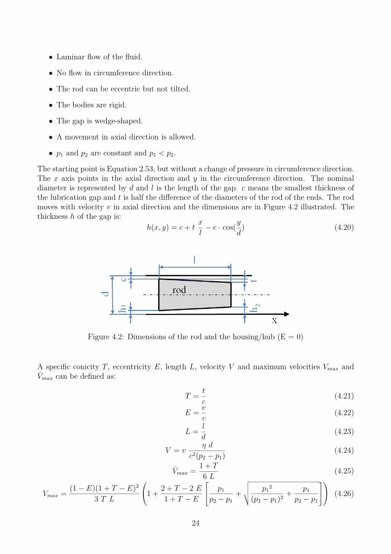
The starting point is Equation 2.53, but without a change of pressure in circumference direction.The x axis points in the axial direction and y in the circumference direction. The nominaldiameter is represented by d and l is the length of the gap. c means the smallest thickness ofthe lubrication gap and t is half the difference of the diameters of the rod of the ends. The rodmoves with velocity v in axial direction and the dimensions are in Figure 4.2 illustrated. Thethickness h of the gap is:

h(x, y) = c+ tx

l− e · cos(y

d) (4.20)

Figure 4.2: Dimensions of the rod and the housing/hub (E = 0)

A specific conicity T , eccentricity E, length L, velocity V and maximum velocities Vmax andVmax can be defined as:

T = t

c(4.21)

E = e

c(4.22)

L = l

d(4.23)

V = vη d

c2(p2 − p1) (4.24)

Vmax = 1 + T

6 L (4.25)

Vmax = (1− E)(1 + T − E)2

3 T L

1 + 2 + T − 2 E1 + T − E

p1

p2 − p1+

√√√√ p12

(p2 − p1)2 + p1

p2 − p1

(4.26)

24

The increase of the rod velocity opposite to the x direction decreases the stiffness of the bearing.Vmax represents the specific velocity, where the stiffness is zero. This means that maximumload capacity in radial direction is zero. S represents the dimensionless stiffness of the bearing.The equation with Vmax can be evaluated by differentiation of the following equation:

S∣∣∣E=0

= 2 T L

(2 + T )2

(1− 6 V L

1 + T

)(4.27)

The second limiting value is Vmax. It denotes the limit before reaching underpressure.

With dynamic viscosity η, the real maximum velocities are determinable by:

vmax = Vmaxc2 (p2 − p1)

η d(4.28)

vmax = Vmaxc2 (p2 − p1)

η d(4.29)

p1 is the lower pressure and p2 is the higher one with gap thickness of the low pressure sideh1 and thickness of the high pressure side h2. The pressure distribution p of any position asfunction of the thickness h:

p = p1 + (p2 − p1)

1h2 −

1h1

2

1h1

2 + 1h2

2

+ 6 η l vt

(1h− 1h1

)(1h− 1h2

)1h1

+ 1h2

(4.30)

The first term is a Poiseuille term caused by pressure gradient and the second one is a Couetteterm provoked by the moving rod. The bearing strength can be calculated by integration ofEquation 4.30 over the surface. The specific/dimensionless form of the load capacity:

F = L T

E

2 + T√(2 + T )2 − 4 E2

− 1−

24 V L2

T E

√

(1 + T )2 − E2 −√

1− E2

T− 2 + T√

(2 + T )2 − 4 E2

(4.31)

The first term depends on the pressure and the second one on the velocity and the pressure.The specific load capacity multiplied by the lateral surface and the pressure difference is theload capacity in Newton:

f = Fd2 π

4 (p2 − p1) (4.32)

The volume flow q through the gap can be calculated with this equation:

q = c3 π (p2 − p1)12 η L

2 (1 + T )2

2 + T+ 3 (2 + T ) E2

4 + T 4

8 (2 + T )

2 + T√(2 + T )2 − 4 E2

− 1(4.33)

The equation is valid for stagnant rod and housing and the unit is cubic meters per second.With knowledge of the diameters of the cross section of the gap the mean velocity of the fluidvfluid can be expressed as:

vfluid = q

Across section= 4 q

(dhousing2 − drod2) π(4.34)

25

4.2.2 Results with nominal ParametersThe results of one bearing with a nominal diameter d = 10 mm and a length l = 18 mm aresummarized in this section. The thinnest gap is c(E = 0) = 50 µm and half the difference ofdiameters of the rod is t = 30 µm. The pressure difference is p2− p1 = 50 bar− 0 bar = 50 bar.The expected dynamic viscosity of the used oil is η = 85 Pa · s. For the calculations twovariables are varied. On the one hand the velocity of the rod from −5 m/s to +5 m/s and onthe other hand the eccentricity varies.

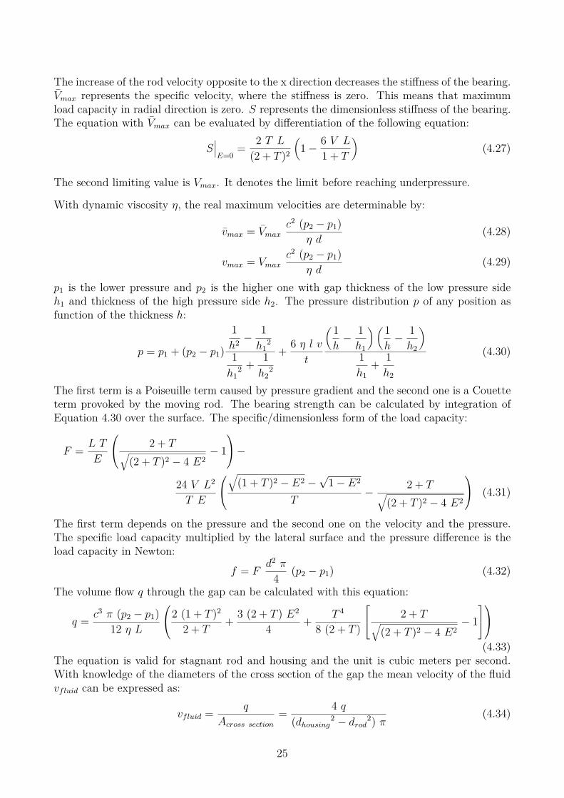
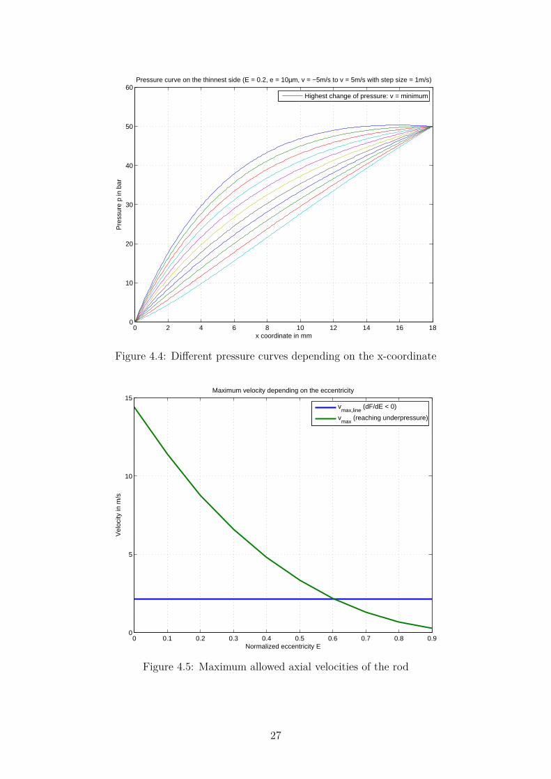
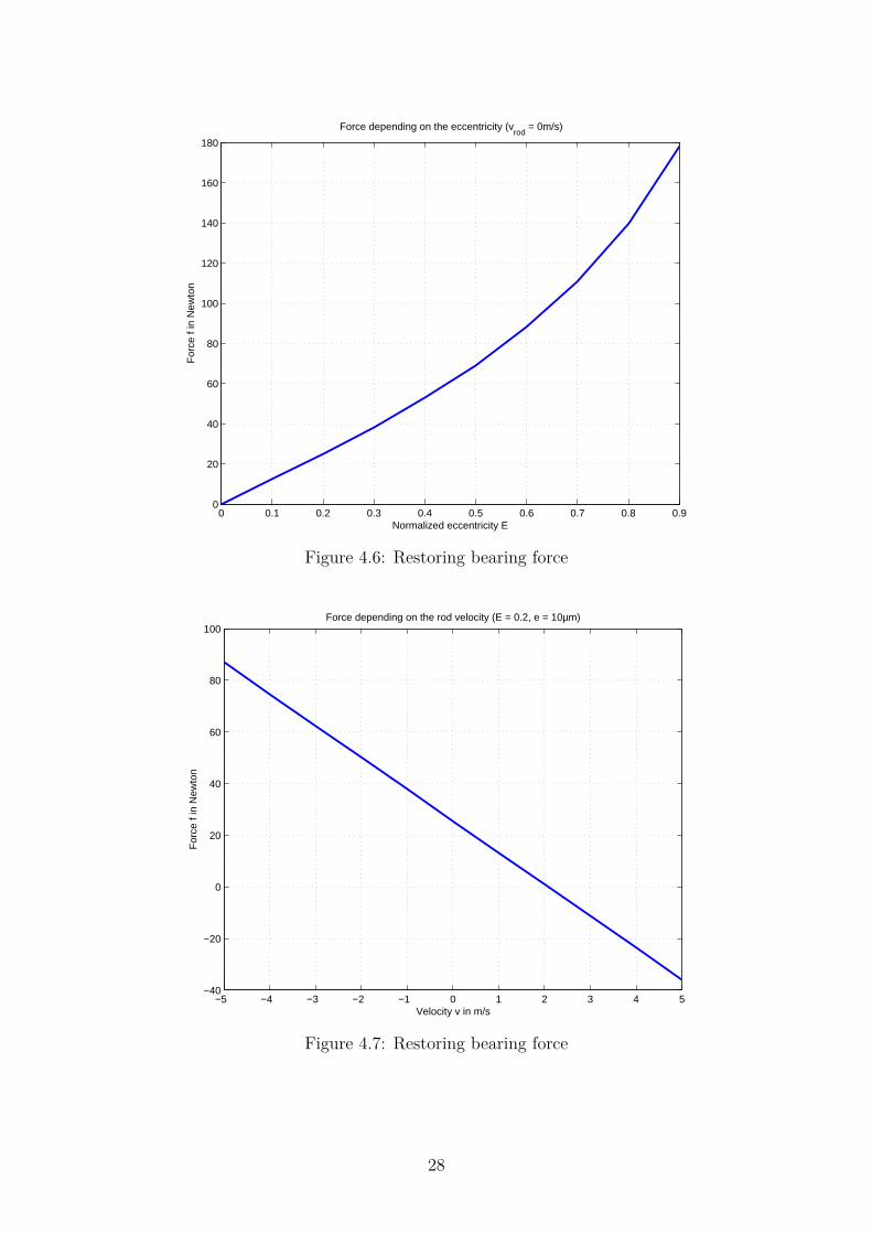
Figures 4.3 and 4.4 show the pressure curves depending on the x-coordinate. On the right sidethere is high pressure and on the left is low pressure.The maximum allowed velocities are displayed in Figure 4.5. vmax does not depend on theeccentricity in contrast to vmax.In Figure 4.6 and 4.7 the radial restoring force is plotted. The force increases disproportionatewith rising eccentricity and proportional with rising rod velocity.The stiffness s shown in Figure 4.8 is falling, if the velocity rises. The limiting value of thestiffness is 0.Figure 4.9 points the volume flow of the fluid in the gap. There is an approximate flow of2.09 cm3/s, if the rod is in the center and increases more than proportional with growingeccentricity.

0 2 4 6 8 10 12 14 16 180

10

20

30

40

50

60

Pressure curve on the thinnest side (vrod

= 0m/s, E = 0 to E = 0.9 with step size = 0.1)

x coordinate in mm

Pre

ssur

e in

bar

Most uniform change of pressure: E = 0

Figure 4.3: Different pressure curves depending on the x-coordinate

26

0 2 4 6 8 10 12 14 16 180

10

20

30

40

50

60Pressure curve on the thinnest side (E = 0.2, e = 10µm, v = −5m/s to v = 5m/s with step size = 1m/s)

x coordinate in mm

Pre

ssur

e p

in b

ar

Highest change of pressure: v = minimum

Figure 4.4: Different pressure curves depending on the x-coordinate

0 0.1 0.2 0.3 0.4 0.5 0.6 0.7 0.8 0.90

5

10

15Maximum velocity depending on the eccentricity

Normalized eccentricity E

Vel

ocity

in m

/s

v

max,line (dF/dE < 0)

vmax

(reaching underpressure)

Figure 4.5: Maximum allowed axial velocities of the rod

27

0 0.1 0.2 0.3 0.4 0.5 0.6 0.7 0.8 0.90

20

40

60

80

100

120

140

160

180

Force depending on the eccentricity (vrod

= 0m/s)


For

ce f

in N

ewto

n

Figure 4.6: Restoring bearing force

−5 −4 −3 −2 −1 0 1 2 3 4 5−40

−20

0

20

40

60

80

100Force depending on the rod velocity (E = 0.2, e = 10µm)

Velocity v in m/s

For

ce f

in N

ewto

n

Figure 4.7: Restoring bearing force

28

−5 −4 −3 −2 −1 0 1 2 3 4 5−4

−2

0

2

4

6

8

10Bearing stiffness s (E = 0, e = 0µm)

Velocity in m/s

Stif

fnes

s s

in N

/µm

Figure 4.8: Stiffness of the bearing

0 0.1 0.2 0.3 0.4 0.5 0.6 0.7 0.8 0.92

2.2

2.4

2.6

2.8

3

3.2

3.4

3.6

3.8

Volume flow depending on the eccentricity (vrod

= 0m/s)


Vol

ume

flow

q in

cm

3 /s

Figure 4.9: Leakage oil

29

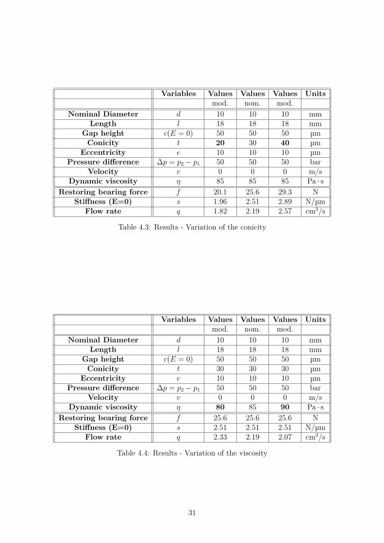
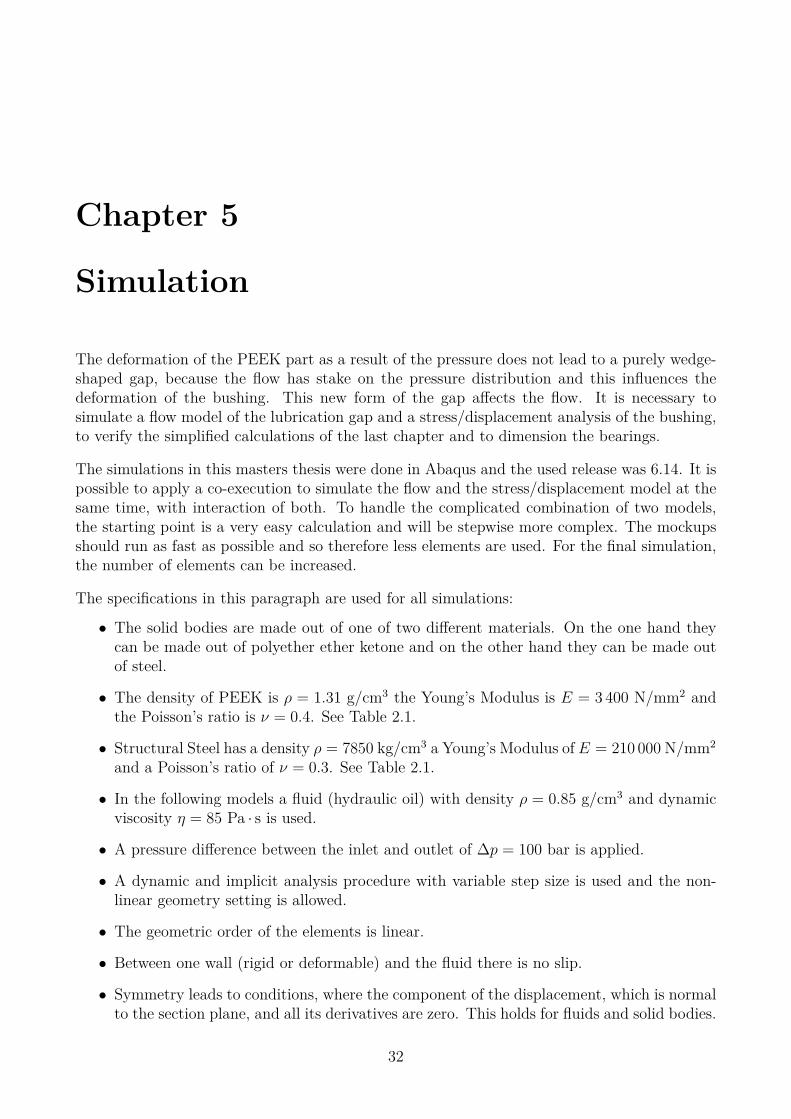
4.2.3 Results with deviant ParametersIn Table 4.1 to 4.4 the results of the calculation of one bearing is given to study a characteristicdeviation of some parameters. These investigations include the variation of the length and theheight of the gap and a change of the conicity and dynamic viscosity. The variations show theimpacts of parameter deviations to the restoring bearing force, the stiffness and the flow rate.The survey is useful to compare a mathematical model and the real prototype.

Variables Values Values Values Unitsmod. nom. mod.

Nominal Diameter d 10 10 10 mmLength l 15 18 21 mm

Gap height c(E = 0) 50 50 50 µmConicity t 30 30 30 µm

Eccentricity e 10 10 10 µmPressure difference ∆p = p2 − p1 50 50 50 bar

Velocity v 0 0 0 m/sDynamic viscosity η 80 85 90 Pa · s

Restoring bearing force f 21.3 25.6 29.8 NStiffness (E=0) s 2.1 2.51 2.93 N/µm

Flow rate q 2.63 2.19 1.88 cm3/s

Table 4.1: Results - Variation of the bearing length







Flow rate q 1.29 2.19 3.42 cm3/s

Table 4.2: Results - Variation of the gap height

30







Flow rate q 1.82 2.19 2.57 cm3/s

Table 4.3: Results - Variation of the conicity







Flow rate q 2.33 2.19 2.07 cm3/s

Table 4.4: Results - Variation of the viscosity

31

Chapter 5

Simulation

The deformation of the PEEK part as a result of the pressure does not lead to a purely wedge-shaped gap, because the flow has stake on the pressure distribution and this influences thedeformation of the bushing. This new form of the gap affects the flow. It is necessary tosimulate a flow model of the lubrication gap and a stress/displacement analysis of the bushing,to verify the simplified calculations of the last chapter and to dimension the bearings.

The simulations in this masters thesis were done in Abaqus and the used release was 6.14. It ispossible to apply a co-execution to simulate the flow and the stress/displacement model at thesame time, with interaction of both. To handle the complicated combination of two models,the starting point is a very easy calculation and will be stepwise more complex. The mockupsshould run as fast as possible and so therefore less elements are used. For the final simulation,the number of elements can be increased.

The specifications in this paragraph are used for all simulations:

• The solid bodies are made out of one of two different materials. On the one hand theycan be made out of polyether ether ketone and on the other hand they can be made outof steel.

• The density of PEEK is ρ = 1.31 g/cm3 the Young’s Modulus is E = 3 400 N/mm2 andthe Poisson’s ratio is ν = 0.4. See Table 2.1.

• Structural Steel has a density ρ = 7850 kg/cm3 a Young’s Modulus of E = 210 000 N/mm2

and a Poisson’s ratio of ν = 0.3. See Table 2.1.

• In the following models a fluid (hydraulic oil) with density ρ = 0.85 g/cm3 and dynamicviscosity η = 85 Pa · s is used.

• A pressure difference between the inlet and outlet of ∆p = 100 bar is applied.

• A dynamic and implicit analysis procedure with variable step size is used and the non-linear geometry setting is allowed.

• The geometric order of the elements is linear.

• Between one wall (rigid or deformable) and the fluid there is no slip.

• Symmetry leads to conditions, where the component of the displacement, which is normalto the section plane, and all its derivatives are zero. This holds for fluids and solid bodies.

32

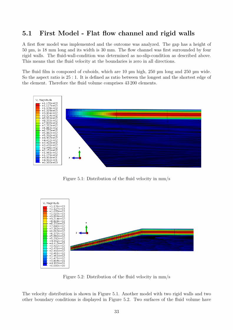
5.1 First Model - Flat flow channel and rigid wallsA first flow model was implemented and the outcome was analyzed. The gap has a height of50 µm, is 18 mm long and its width is 30 mm. The flow channel was first surrounded by fourrigid walls. The fluid-wall-condition was determined as no-slip-condition as described above.This means that the fluid velocity at the boundaries is zero in all directions.

The fluid film is composed of cuboids, which are 10 µm high, 250 µm long and 250 µm wide.So the aspect ratio is 25 : 1. It is defined as ratio between the longest and the shortest edge ofthe element. Therefore the fluid volume comprises 43 200 elements.

Figure 5.1: Distribution of the fluid velocity in mm/s

Figure 5.2: Distribution of the fluid velocity in mm/s

The velocity distribution is shown in Figure 5.1. Another model with two rigid walls and twoother boundary conditions is displayed in Figure 5.2. Two surfaces of the fluid volume have

33

symmetry conditions: The displacements and the velocities in main flow direction (x) and indirection of the height of the gap (y) are allowed to be unequal to zero. Both figures show thestationary situation after 10 increments (10 µs) of calculation.

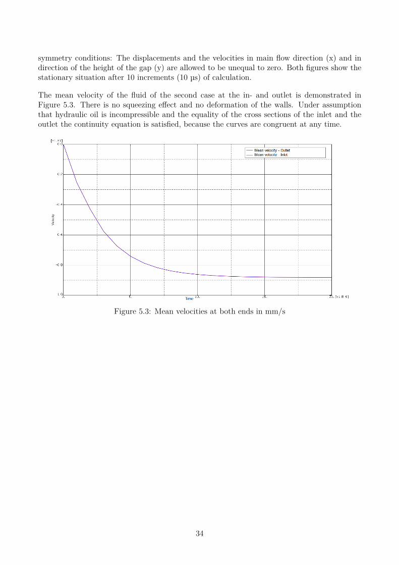
The mean velocity of the fluid of the second case at the in- and outlet is demonstrated inFigure 5.3. There is no squeezing effect and no deformation of the walls. Under assumptionthat hydraulic oil is incompressible and the equality of the cross sections of the inlet and theoutlet the continuity equation is satisfied, because the curves are congruent at any time.

Figure 5.3: Mean velocities at both ends in mm/s

34

5.2 Second Model - Flat flow channel and one deforma-ble, both-sided fixed wall

5.2.1 Setup AThe next step is to evolve a CFD model that interacts with a deformable body. The heightof the fluid gap is 2 mm. With a thicker gap, the ratios of the edge lengths of the elementsare better. With aspect ratios close to one, the elements are cube-like. Otherwise they are flator long shaped. The simulations showed that cube-like elements are robust despite numericalerrors, cause less errors when the elements gets deformed and provide better results.

The gap length is 18 mm and it is 30 mm wide. On the top of the gap there is an interactionsurface, that allows to combine the simulations of a fluid and a solid body. The thickness of thedeformable body is 5 mm and it is made out of PEEK. At the bottom of the fluid there is a rigidwall. The left and the right boundaries are symmetry boundaries, where the displacement andthe velocity in z direction is zero. For interacting simulations a fluid-structure co-simulationboundary is needed. The body is pinned on the inlet and outlet side. The left and right sideshave the same symmetry conditions like the fluid. The dynamic viscosity is a thousand timesbigger than the real value. η is 8500 Pa · s. This increase of the viscosity should lead to smallermean fluid velocity. A bigger gap height leads to a higher flow velocity by reason that vmean isproportional to h3, where h means the height of the lubrication gap. The other properties arethe same like above.

The discrete fluid model consists of cuboids, which are 250 µm high, 500 µm long and 500 µmwide. So the aspect ratio is 2 : 1. And the body model has cuboids with a height of 625 µm.The length and the width are the same like the other model. The ratio is 1.25 : 1. The numberof elements is 17 280 for both parts.

Instable simulations are possible, due to the fact that every model has numerical errors andthis errors are also transferred to each other model. So as a energy dissipation mechanism adamping property for the model of the body can be implemented. In this case it is definedas a so called Rayleigh damping. It is a linear combination of mass and stiffness matrix. Theeigenvectors of the damped and the undamped system are the same. To get a model with ashort settling time, the damping ratio ζi of the mode i is useful. It is defined as:

ζi = αR2 ωi

+ βR ωi2 (5.1)

Figure 5.4 is a comparison of three different co-simulations with implemented Rayleigh dam-ping. The usage of the reduced integration provokes solutions with increasing oscillations. Fullintegration diminishes the oscillations, but can not prevent it. Higher damping coefficientsshould derate oscillating and instable solutions. And, in fact, the oscillations disappear. Thefirst trials of the dynamic analysis used damping coefficients of αR = 200 1/s and βR = 4 · 10−6 s.The raised coefficients were 1.5 times higher: αR = 300 1/s and βR = 6 · 10−6 s.

ωi means the natural frequency at this mode. αR defines the mass proportional damping andcushions the lower frequencies. βR fixes the stiffness proportional damping and cushions thehigher frequencies. To determine the right values of the coefficients the step response of acantilever beam was studied. [32] [33] [34]

35

Figure 5.4: Procedures to avoid oscillations

5.2.2 Setup BThe following simulation setup is similar to the last one. There is one deformable wall, but theviscosity is set to the normal value of η = 85 Pa · s and the dimensions are: The Gap height isreduced to 200 µm, the length is 18 mm and the width is only 2 mm. For reasons of dimensionalsimilarity, there is no change of velocity and pressure in z direction expected. The thicknessof the deformable body is 5 mm and it is made out of PEEK. The damping coefficients areαR = 600 1/s and βR = 8 · 10−6 s.

Figure 5.5: Influence of different numbers of elements in y direction

To determine the influence of the number of elements in y direction on the flow profile, twosimulations with 8 and 16 elements in y directions were done and matched in Figure 5.5. Thefluid voxels are 25 µm and 12.5 µm high, and the length and the width are the same like above.

36

So the aspect ratios are 10 : 1 or 20 : 1 and the patterns include 1152 or 2304 elements. Thesolid body model is unchanged for both simulation attempts. There are 1152 elements with aratio of 2 : 1.

There is a difference between the two simulations during the settling process, but the statio-nary solution is equal. Two explanations are possible for the difference. The first is a betterapproximation of the flow profile, by using more elements and the second one is the discrepancyof the aspect ratios. A first reference point of the aspect ratio limit is the recommended limitfor the selection criteria of shape metrics in Abaqus to verify the mesh. It is 10. [35]

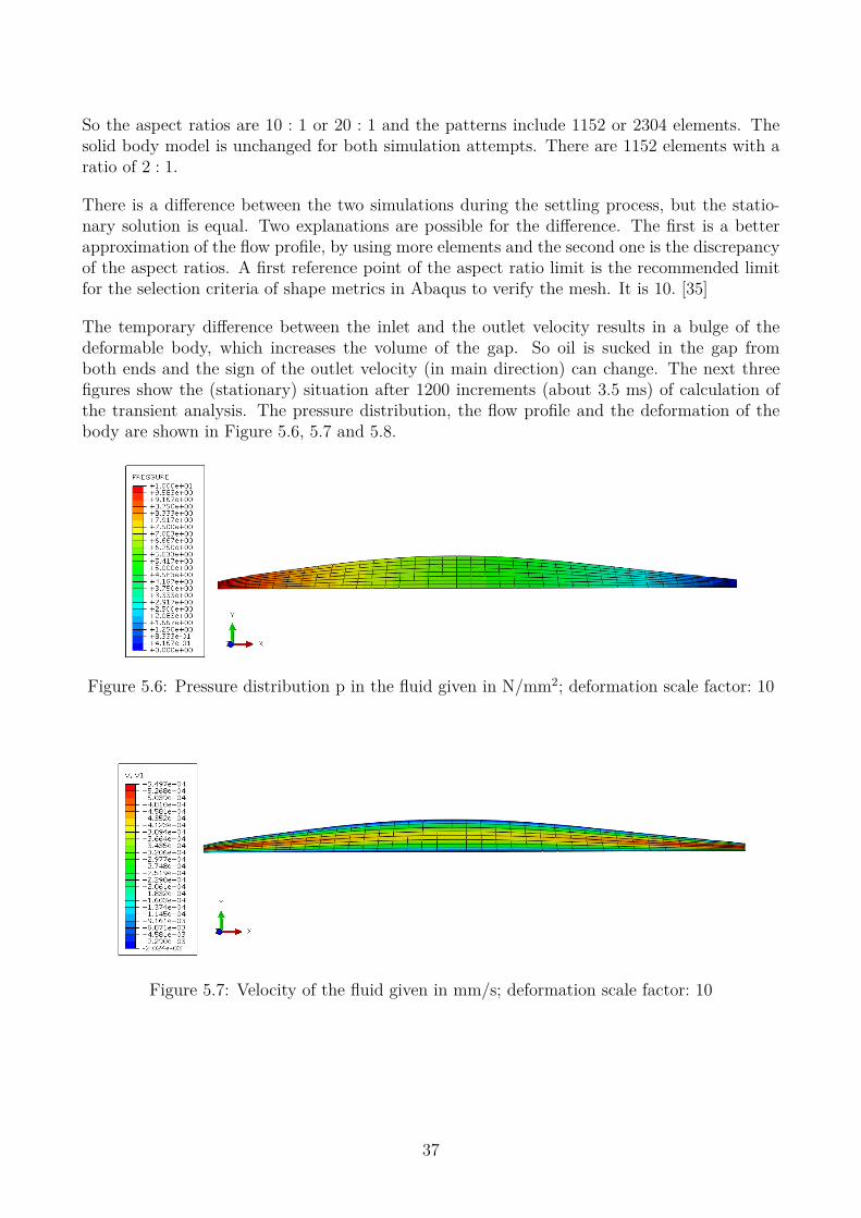
The temporary difference between the inlet and the outlet velocity results in a bulge of thedeformable body, which increases the volume of the gap. So oil is sucked in the gap fromboth ends and the sign of the outlet velocity (in main direction) can change. The next threefigures show the (stationary) situation after 1200 increments (about 3.5 ms) of calculation ofthe transient analysis. The pressure distribution, the flow profile and the deformation of thebody are shown in Figure 5.6, 5.7 and 5.8.

Figure 5.6: Pressure distribution p in the fluid given in N/mm2; deformation scale factor: 10

Figure 5.7: Velocity of the fluid given in mm/s; deformation scale factor: 10

37

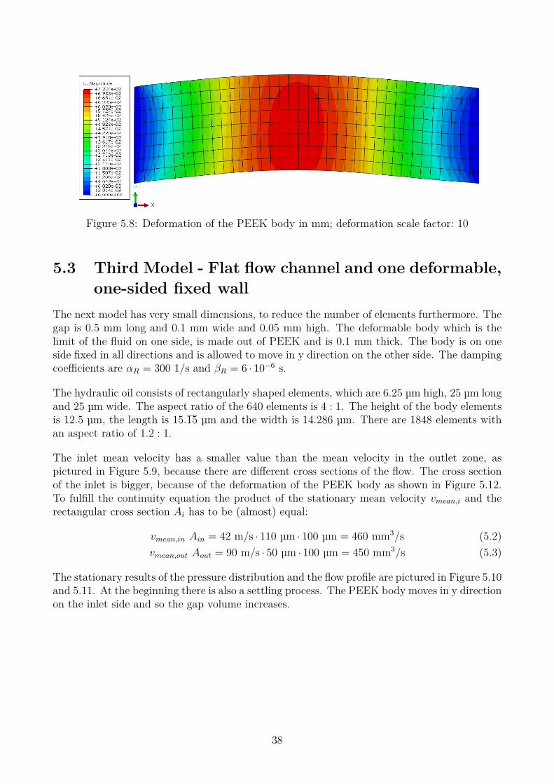
Figure 5.8: Deformation of the PEEK body in mm; deformation scale factor: 10

5.3 Third Model - Flat flow channel and one deformable,one-sided fixed wall

The next model has very small dimensions, to reduce the number of elements furthermore. Thegap is 0.5 mm long and 0.1 mm wide and 0.05 mm high. The deformable body which is thelimit of the fluid on one side, is made out of PEEK and is 0.1 mm thick. The body is on oneside fixed in all directions and is allowed to move in y direction on the other side. The dampingcoefficients are αR = 300 1/s and βR = 6 · 10−6 s.

The hydraulic oil consists of rectangularly shaped elements, which are 6.25 µm high, 25 µm longand 25 µm wide. The aspect ratio of the 640 elements is 4 : 1. The height of the body elementsis 12.5 µm, the length is 15.15 µm and the width is 14.286 µm. There are 1848 elements withan aspect ratio of 1.2 : 1.

The inlet mean velocity has a smaller value than the mean velocity in the outlet zone, aspictured in Figure 5.9, because there are different cross sections of the flow. The cross sectionof the inlet is bigger, because of the deformation of the PEEK body as shown in Figure 5.12.To fulfill the continuity equation the product of the stationary mean velocity vmean,i and therectangular cross section Ai has to be (almost) equal:

vmean,in Ain = 42 m/s · 110 µm · 100 µm = 460 mm3/s (5.2)vmean,out Aout = 90 m/s · 50 µm · 100 µm = 450 mm3/s (5.3)

The stationary results of the pressure distribution and the flow profile are pictured in Figure 5.10and 5.11. At the beginning there is also a settling process. The PEEK body moves in y directionon the inlet side and so the gap volume increases.

38

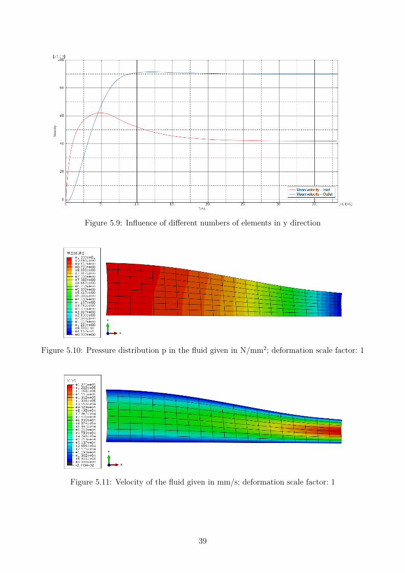
Figure 5.9: Influence of different numbers of elements in y direction

Figure 5.10: Pressure distribution p in the fluid given in N/mm2; deformation scale factor: 1


39

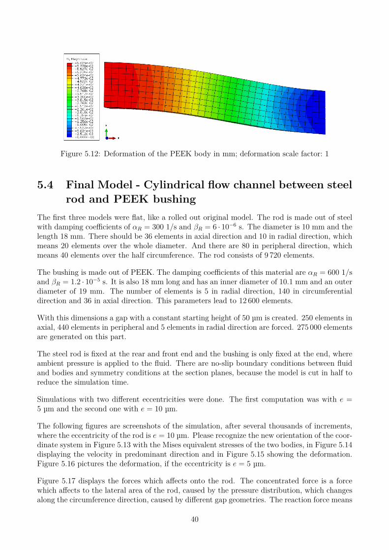
Figure 5.12: Deformation of the PEEK body in mm; deformation scale factor: 1

5.4 Final Model - Cylindrical flow channel between steelrod and PEEK bushing

The first three models were flat, like a rolled out original model. The rod is made out of steelwith damping coefficients of αR = 300 1/s and βR = 6 · 10−6 s. The diameter is 10 mm and thelength 18 mm. There should be 36 elements in axial direction and 10 in radial direction, whichmeans 20 elements over the whole diameter. And there are 80 in peripheral direction, whichmeans 40 elements over the half circumference. The rod consists of 9 720 elements.

The bushing is made out of PEEK. The damping coefficients of this material are αR = 600 1/sand βR = 1.2 · 10−5 s. It is also 18 mm long and has an inner diameter of 10.1 mm and an outerdiameter of 19 mm. The number of elements is 5 in radial direction, 140 in circumferentialdirection and 36 in axial direction. This parameters lead to 12 600 elements.

With this dimensions a gap with a constant starting height of 50 µm is created. 250 elements inaxial, 440 elements in peripheral and 5 elements in radial direction are forced. 275 000 elementsare generated on this part.

The steel rod is fixed at the rear and front end and the bushing is only fixed at the end, whereambient pressure is applied to the fluid. There are no-slip boundary conditions between fluidand bodies and symmetry conditions at the section planes, because the model is cut in half toreduce the simulation time.

Simulations with two different eccentricities were done. The first computation was with e =5 µm and the second one with e = 10 µm.

The following figures are screenshots of the simulation, after several thousands of increments,where the eccentricity of the rod is e = 10 µm. Please recognize the new orientation of the coor-dinate system in Figure 5.13 with the Mises equivalent stresses of the two bodies, in Figure 5.14displaying the velocity in predominant direction and in Figure 5.15 showing the deformation.Figure 5.16 pictures the deformation, if the eccentricity is e = 5 µm.

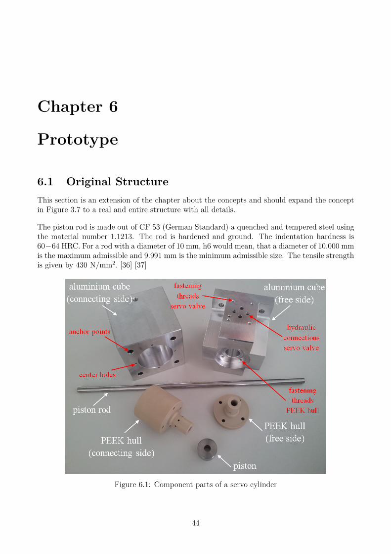
Figure 5.17 displays the forces which affects onto the rod. The concentrated force is a forcewhich affects to the lateral area of the rod, caused by the pressure distribution, which changesalong the circumference direction, caused by different gap geometries. The reaction force means

40

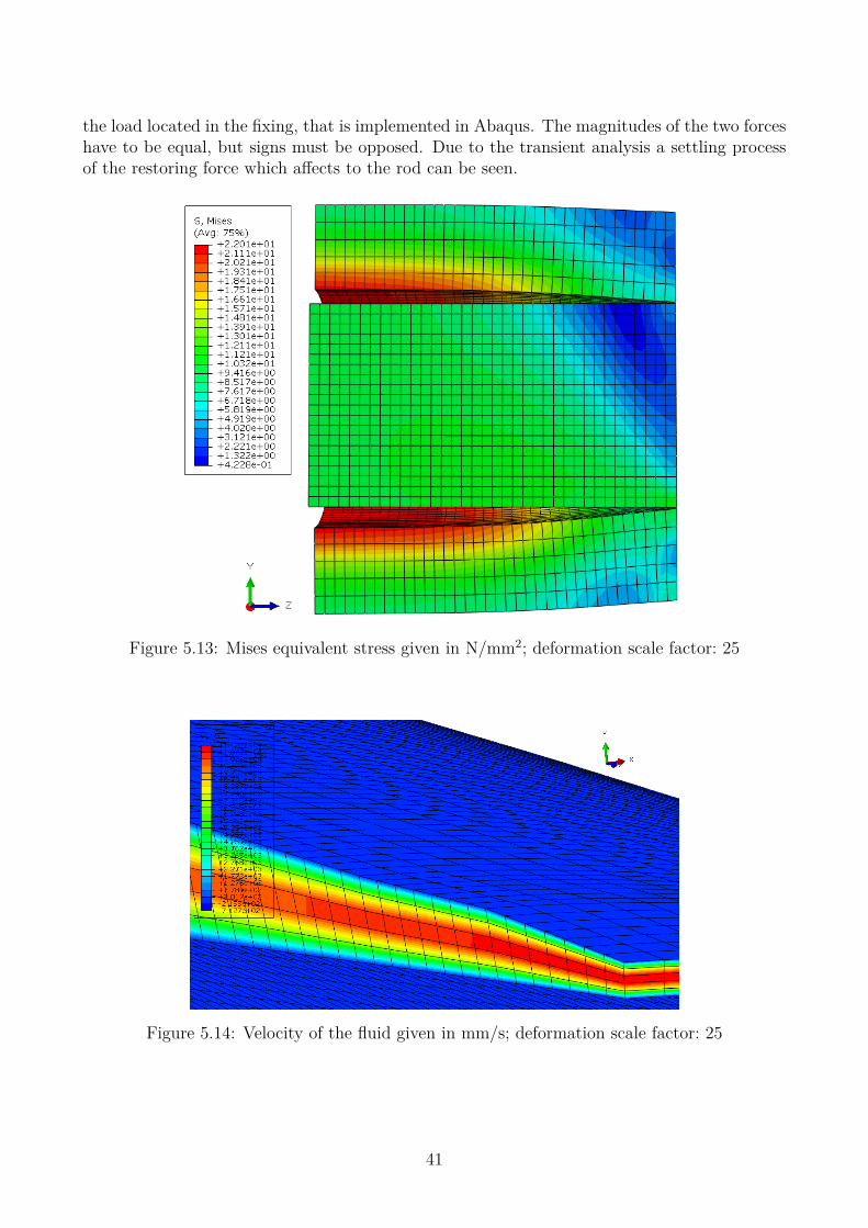
the load located in the fixing, that is implemented in Abaqus. The magnitudes of the two forceshave to be equal, but signs must be opposed. Due to the transient analysis a settling processof the restoring force which affects to the rod can be seen.

Figure 5.13: Mises equivalent stress given in N/mm2; deformation scale factor: 25


41

Figure 5.15: Deformation in mm; e = 10 µm ; deformation scale factor: 25

Figure 5.16: Deformation in mm; e = 5 µm ;deformation scale factor: 10

42

Figure 5.17: Concentrated and reaction forces in Newton

43

Chapter 6

Prototype

6.1 Original StructureThis section is an extension of the chapter about the concepts and should expand the conceptin Figure 3.7 to a real and entire structure with all details.

The piston rod is made out of CF 53 (German Standard) a quenched and tempered steel usingthe material number 1.1213. The rod is hardened and ground. The indentation hardness is60−64 HRC. For a rod with a diameter of 10 mm, h6 would mean, that a diameter of 10.000 mmis the maximum admissible and 9.991 mm is the minimum admissible size. The tensile strengthis given by 430 N/mm2. [36] [37]

Figure 6.1: Component parts of a servo cylinder

44

The piston is made out of quenched and tempered steel 42CrMo4 (German Standard) with thematerial number 1.7225. The tensile strength is given by 750 N/mm2. [38]

To ensure a suitable tight fit of piston and piston rod, the used fits are calculated in Section 4.1.The limits of the inner diameter of the piston are 9.986 mm and 9.975 mm. To shrink-fit thepiston, it must be heated to 230 K + Tambient.

The outer diameter limits of the piston are 29.993 mm respectively 29.980 mm. There shouldbe chamfers on both sides of the outer girthed area because it influences the friction. Thediameter of the piston chamber is between 30.021 mm and 30.000 mm. A gap of 7 µm to 41µmis placed.

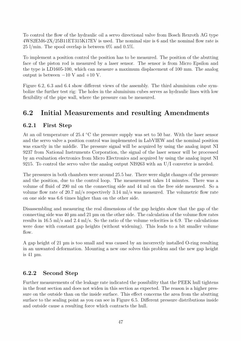
Figure 6.2: General view of the assembly with one extra aluminium cube

The drill hole in which the piston rod is admitted has a diameter inside the limits of 10.040 mmto 10.050 mm. Piston rod and (PEEK) hull have dimensions which ensure that the gap withlubrication film has a height of 40 µm to 59 µm.

The bearing hulls are embedded in the aluminium housing. The aluminium cubes contain alsopower, tank and leakage connections, the servo valve connection holes and different holes todirect the hydraulic fluid.

Surfaces being moved relative to each other should be as smooth as possible to reduce friction.The touching surfaces of rod/hull and piston/housing are affected.

For designs of sealing points dimensions of grooves, tolerances and other guidelines are taken

45

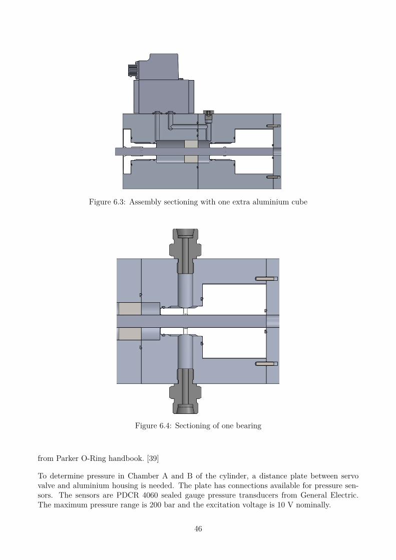
Figure 6.3: Assembly sectioning with one extra aluminium cube

Figure 6.4: Sectioning of one bearing

from Parker O-Ring handbook. [39]

To determine pressure in Chamber A and B of the cylinder, a distance plate between servovalve and aluminium housing is needed. The plate has connections available for pressure sen-sors. The sensors are PDCR 4060 sealed gauge pressure transducers from General Electric.The maximum pressure range is 200 bar and the excitation voltage is 10 V nominally.

46

To control the flow of the hydraulic oil a servo directional valve from Bosch Rexroth AG type4WS2EM6-2X/25B11ET315K17EV is used. The nominal size is 6 and the nominal flow rate is25 l/min. The spool overlap is between 0% and 0.5%.

To implement a position control the position has to be measured. The position of the abuttingface of the piston rod is measured by a laser sensor. The sensor is from Micro Epsilon andthe type is LD1605-100, which can measure a maximum displacement of 100 mm. The analogoutput is between −10 V and +10 V.

Figure 6.2, 6.3 and 6.4 show different views of the assembly. The third aluminium cube sym-bolize the further test rig: The holes in the aluminium cubes serves as hydraulic lines with lowflexibility of the pipe wall, where the pressure can be measured.

6.2 Initial Measurements and resulting Amendments

6.2.1 First StepAt an oil temperature of 25.4 ◦C the pressure supply was set to 50 bar. With the laser sensorand the servo valve a position control was implemented in LabVIEW and the nominal positionwas exactly in the middle. The pressure signal will be acquired by using the analog input NI9237 from National Instruments Corporation, the signal of the laser sensor will be processedby an evaluation electronics from Micro Electronics and acquired by using the analog input NI9215. To control the servo valve the analog output NI9263 with an U/I converter is needed.

The pressures in both chambers were around 25.5 bar. There were slight changes of the pressureand the position, due to the control loop. The measurement takes 14 minutes. There was avolume of fluid of 290 ml on the connecting side and 44 ml on the free side measured. So avolume flow rate of 20.7 ml/s respectively 3.14 ml/s was measured. The volumetric flow rateon one side was 6.6 times higher than on the other side.

Disassembling and measuring the real dimensions of the gap heights show that the gap of theconnecting side was 40 µm and 21 µm on the other side. The calculation of the volume flow ratesresults in 16.5 ml/s and 2.4 ml/s. So the ratio of the volume velocities is 6.9. The calculationswere done with constant gap heights (without widening). This leads to a bit smaller volumeflow.

A gap height of 21 µm is too small and was caused by an incorrectly installed O-ring resultingin an unwanted deformation. Mounting a new one solves this problem and the new gap heightis 41 µm.

6.2.2 Second StepFurther measurements of the leakage rate indicated the possibility that the PEEK hull tightensin the front section and does not widen in this section as expected. The reason is a higher pres-sure on the outside than on the inside surface. This effect concerns the area from the abuttingsurface to the sealing point as you can see in Figure 6.5. Different pressure distributions insideand outside cause a resulting force which contracts the hull.

47

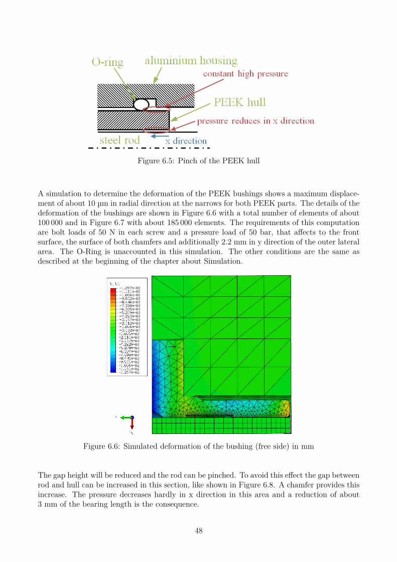
Figure 6.5: Pinch of the PEEK hull

A simulation to determine the deformation of the PEEK bushings shows a maximum displace-ment of about 10 µm in radial direction at the narrows for both PEEK parts. The details of thedeformation of the bushings are shown in Figure 6.6 with a total number of elements of about100 000 and in Figure 6.7 with about 185 000 elements. The requirements of this computationare bolt loads of 50 N in each screw and a pressure load of 50 bar, that affects to the frontsurface, the surface of both chamfers and additionally 2.2 mm in y direction of the outer lateralarea. The O-Ring is unaccounted in this simulation. The other conditions are the same asdescribed at the beginning of the chapter about Simulation.

Figure 6.6: Simulated deformation of the bushing (free side) in mm

The gap height will be reduced and the rod can be pinched. To avoid this effect the gap betweenrod and hull can be increased in this section, like shown in Figure 6.8. A chamfer provides thisincrease. The pressure decreases hardly in x direction in this area and a reduction of about3 mm of the bearing length is the consequence.

48

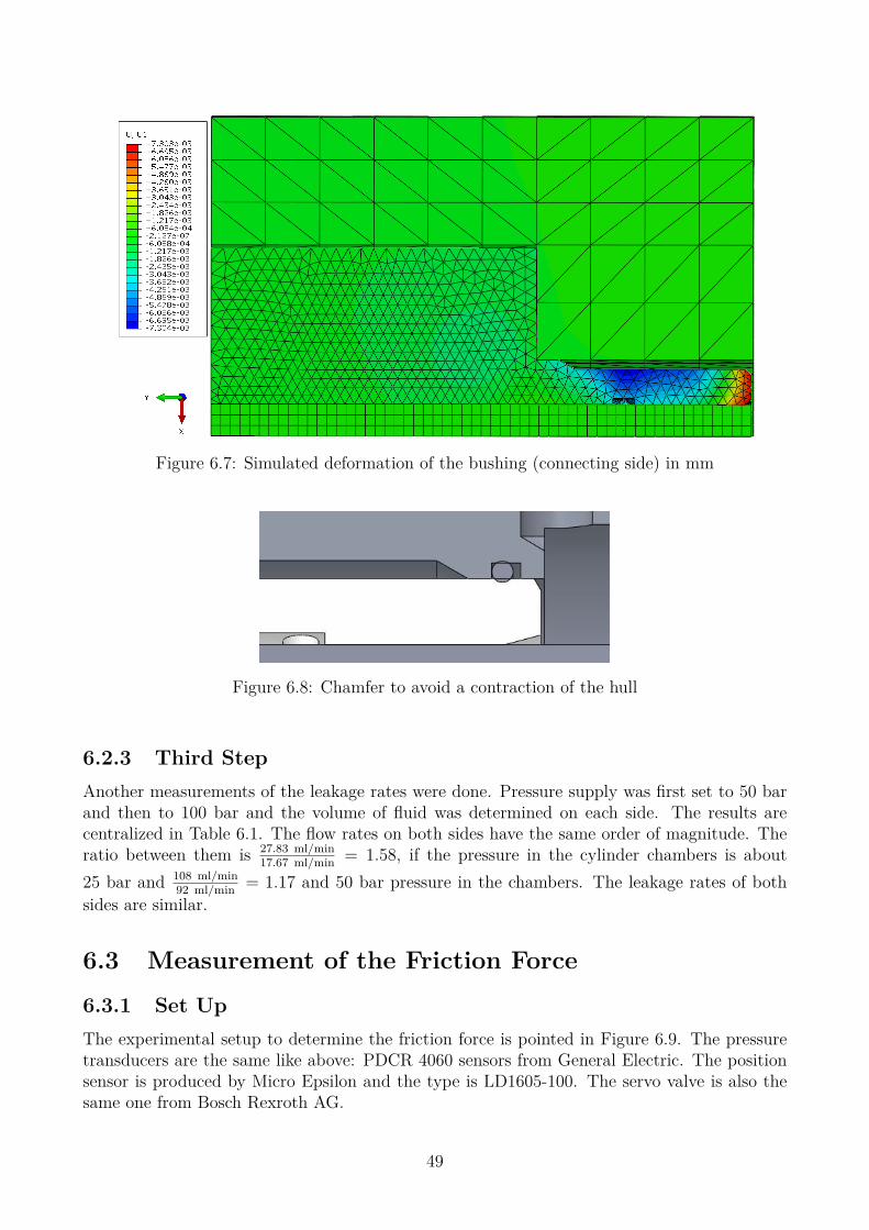
Figure 6.7: Simulated deformation of the bushing (connecting side) in mm

Figure 6.8: Chamfer to avoid a contraction of the hull

6.2.3 Third StepAnother measurements of the leakage rates were done. Pressure supply was first set to 50 barand then to 100 bar and the volume of fluid was determined on each side. The results arecentralized in Table 6.1. The flow rates on both sides have the same order of magnitude. Theratio between them is 27.83 ml/min

17.67 ml/min = 1.58, if the pressure in the cylinder chambers is about25 bar and 108 ml/min

92 ml/min = 1.17 and 50 bar pressure in the chambers. The leakage rates of bothsides are similar.

6.3 Measurement of the Friction Force

6.3.1 Set UpThe experimental setup to determine the friction force is pointed in Figure 6.9. The pressuretransducers are the same like above: PDCR 4060 sensors from General Electric. The positionsensor is produced by Micro Epsilon and the type is LD1605-100. The servo valve is also thesame one from Bosch Rexroth AG.

49

25 bar 25 bar 50 bar 50 barconnecting side free side connecting side free sidepA ≈ 24.5 bar pB ≈ 24.5 bar pA ≈ 49.2 bar pB ≈ 48.6 bar∆t = 3 min ∆t = 3 min ∆t = 2.5 min ∆t = 2.5 minV = 83.5 ml V = 53 ml V = 270 ml V = 230 ml

q = 27.83 ml/min q = 17.67 ml/min q = 108 ml/min q = 92 ml/min

Table 6.1: Measurement of the flow rate of the leakage rate

Figure 6.9: Scheme of the setup

The used LabVIEW program can be seen in Figure 6.10. There are different ways to controlthe servo valve. It is possible to set the position of the valve manually, to set the positionof the cylinder or an automatic presetting of the cylinder position by using a sine wave or arectangular function is possible. The first possibility can not be used to measure the frictionforce.

A closed-loop control is implemented by using a PID controller. The values of the controllerare: Kc = 0.1, Ti = 0.01 min and Td = 0 min. Where Kc means the proportional gain, Tirepresents the integral and Td the derivative time.

The position and both chamber pressures (pA and pB) will be determined. The setpoint positionis sinusoidal, where the offset (means the average value), the magnitude and the frequency canbe adjusted and in case of a rectangular function the duty cycle too.

Figure 6.10 to Figure 6.13 show the LabVIEW-Block diagrams. It is possible to write themeasurements in a file, to save the data. The recording period can be freely chosen. Pressurehistories, control input, setpoint value and actual value of the position are saved. Cancelingthe programm should set the valve to the neutral position.

50

Figure 6.10: Block diagram - LabVIEW

51

Figure 6.11: Alternative detail of the block diagram - Rectangular function

Figure 6.12: Alternative detail of the block diagram - Manually setting - Cylinder

Figure 6.13: Alternative detail of the block diagram - Manually setting - Valve

The clock frequency is set to 4 ms. A substantially faster cycle can be reached by applicationof a Field Programmable Gate Array (FPGA).

Figure 6.11 is a detail which shows the possibility to choose different functions. Here, a sineand a rectangular function are implemented.

It is also possible to set the nominal position value manually. The control unit and the bridging

52

of the automated setting is shown in Figure 6.12. The closed loop tries to hold the positionwhich is indicated.Setting the position of the valve leads to a constant flow till the servo cylinder reaches one of thestop positions. It is used to check the functionality of valve, servo cylinder and bearings. Themanually setting unit and the bridging of the other possibilities are pointed out in Figure 6.13.

6.3.2 Processing of measured DataThe recorded data is cut to make sure that an integer number of periods is available. Otherwisespectral leakage can occur in the following steps. By recording the setpoint and the real valueof the position and the pressures in the chambers and with knowledge of the geometry variousdiagrams can be created. The supply pressure was set to 20 bar. The motion of the cylindershould be sinusoidal. The frequency of the sine wave is 0.1 Hz and the amplitude is 5 mm.

Using Fast Fourier Transformation (FFT) converts a function of time in a function of frequency.The FFT is a special algorithm to determine the Discrete Fourier Transformation. The setpointposition x(t) is transformed to X(f). So the derivation dx(t)

dtcan be converted to an multipli-

cation with j · 2 ·π · f ·X(f). Now the inverse FFT transforms the received velocity V (f) (= j · 2 ·π · f ·X(f)) into v(t) which is a time dependent function. The single side spectrum ofV (f) can be seen in Figure 6.14.

0 20 40 60 80 100 120 1400

0.5

1

1.5

2

2.5

3

3.5

4

Single−Sided Amplitude Spectrum of vist

(t)

Frequency in Hz

|Vis

t(f)|

Figure 6.14: Spectrum of the calculated velocity of the piston

In addition to the peek at 0.1 Hz there are peeks at 25 Hz and its multiples. This additionalpeeks are due to vibration caused by the hydraulic power unit. The rotational velocity of theelectric pump is 1 500 rpm. This means 25 rotations per second. To suppress the additional

53

peeks, to reduce the measurement noise and to smooth the data, the signal can be filtered.A Finite Impulse Response (FIR) filter is used. The used filter is a lowpass and the phaseis linear. The filter has 21 coefficients, a cutoff frequency of 1 Hz and the window type is a“21-point” Kaiser window. The sidelobe attenuation is 0.5. Figure 6.15 shows the frequencyresponse of the filter.

0 0.1 0.2 0.3 0.4 0.5 0.6 0.7 0.8 0.9 1−200

−150

−100

−50

0

50

100

Normalized Frequency (×π rad/sample)

Pha

se (

degr

ees)

0 0.1 0.2 0.3 0.4 0.5 0.6 0.7 0.8 0.9 1−80

−60

−40

−20

0

Normalized Frequency (×π rad/sample)

Mag

nitu

de (

dB)

Figure 6.15: Frequency response of the used lowpass

The friction forces are proportional to the pressure difference because the slow movement ofpiston and rod causes a very low acceleration force:

m x+ FFriction = F∆p (6.1)

The acceleration force can be neglected and above equation turns into:

FFriction = F∆p (6.2)

The dependency of friction and velocity is shown in Figure 6.16. There were several cycles ofsinusoidal movements. The calculated velocities and the appropriate friction forces are displayedas points. We can see both sections where the friction force is approximately constant and astep of the force where v is small or zero. FFriction approximately depends on v in the followingway:

FFriction = c · sign(v) (6.3)Figure 6.16 shows the typical curve of a solid friction.Every experiment consists of at least 20 cycles. Averaging the cycles improves measured dataand provides for clearly arranged diagrams. Figure 6.17 shows the averaged data of Figure 6.16.A time dependent diagram to see position, velocity and friction in one chart is Figure 6.18.

54

−5 −4 −3 −2 −1 0 1 2 3 4 5−15

−10

−5

0

5

10

15

20Friction

Velocity in mm/s

For

ce in

New

ton

Figure 6.16: Friction force of piston and rod

−4 −3 −2 −1 0 1 2 3 4−15

−10

−5

0

5

10

15Friction

Velocity in mm/s

For

ce in

New

ton

Figure 6.17: Mean friction force of piston and rod

55

0 1 2 3 4 5 6 7 8 9 10−15

−10

−5

0

5

10

15Overlay

Time in seconds

Friction Force in NewtonPosition in mmVelocity in mm/s

Figure 6.18: Time behaviour

6.3.3 Friction Force Comparisons with varied ParametersThe measurements of the friction force were done with different parameters. There were severalmagnitudes and frequencies of the specified sine wave-form position.

Series of measurements 1: Supply pressure was varied and set to 20 bar, 40 bar, 60 bar,80 bar and 100 bar. A frequency of 0.2 Hz was applied. The effect of varying the supplypressure is represented by Figure 6.19. The constant value of the magnitude is 5 mm.

Series of measurements 2: The frequency of the sine wave was also 0.2 Hz and the amplitudewas 2.5 mm, 5 mm and 7.5 mm. Bigger magnitudes lead to clearly higher pressure differencesof the cylinder chambers. The variation of the magnitude of the position leads to Figure 6.20at a constant pressure supply of 20 bar.

In each case some different measurements were done. Both diagrams uses mean velocities andmean frictions. At least 20 cycles were measured and the friction forces and the velocities arean average value of these cycles.

The higher the supply pressure, the higher the friction force. The force does not increase pro-portionally. The pressure rises from 20 bar to the five times higher value of 100 bar, but thefriction force has doubled.

Increasing the magnitude induces higher velocities (frequency remaining constant) in Figure 6.20,which explains the stretching effect in x direction. It also increases the friction force.

Both effects can be explained by not ideal geometry. The drillings in the bearings and the

56

cylinder chamber can be slightly tilted or they are not concentric. In both cases a friction forcecan occur, which can not be reduced to zero. The force can be induced by the touching surfacesof piston and housing or by rod and bearings.

−8 −6 −4 −2 0 2 4 6 8−40

−30

−20

−10

0

10

20

30

40Friction

Velocity in mm/s

For

ces

in N

ewto

n

Supply pressure = 20 barSupply pressure = 40 barSupply pressure = 60 barSupply pressure = 80 barSupply pressure = 100 bar

Figure 6.19: Comparison of friction forces with varied supply pressure

−15 −10 −5 0 5 10 15−20

−15

−10

−5

0

5

10

15

20Friction

Velocity in mm/s

For

ces

in N

ewto

n

Magnitude = 2.5 mmMagnitude = 5 mmMagnitude = 7.5 mm

Figure 6.20: Comparison of friction forces with varied magnitude

57

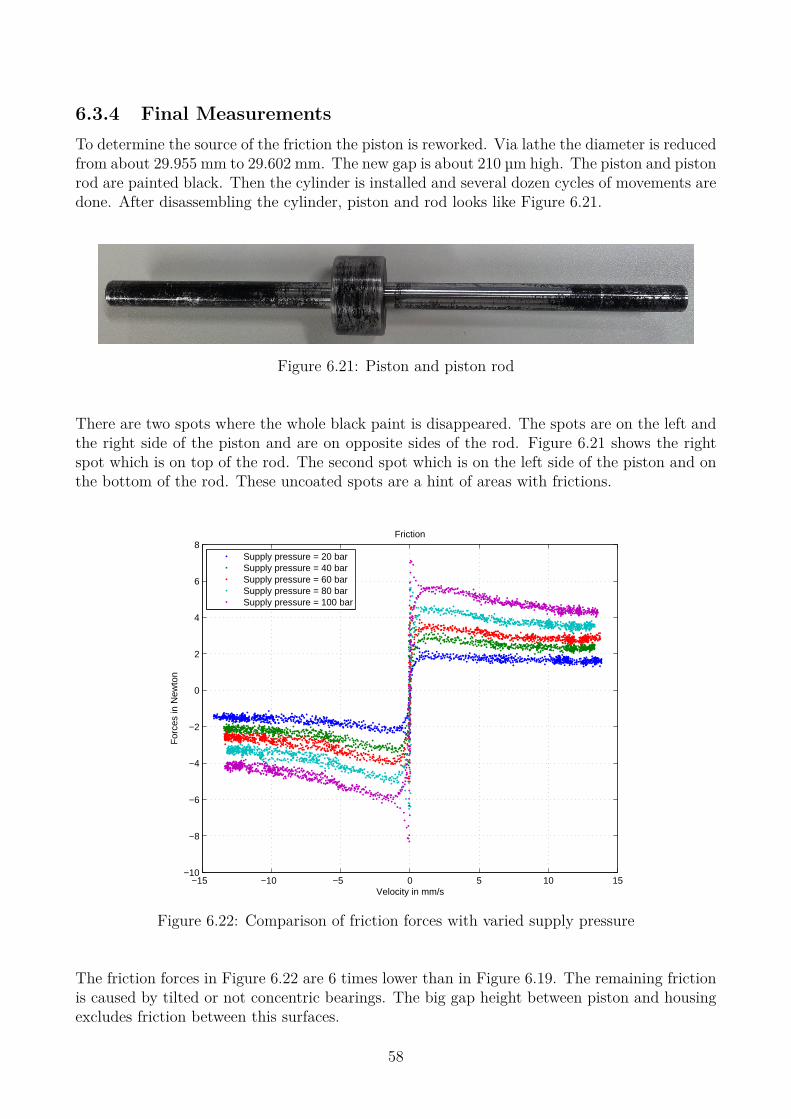
6.3.4 Final MeasurementsTo determine the source of the friction the piston is reworked. Via lathe the diameter is reducedfrom about 29.955 mm to 29.602 mm. The new gap is about 210 µm high. The piston and pistonrod are painted black. Then the cylinder is installed and several dozen cycles of movements aredone. After disassembling the cylinder, piston and rod looks like Figure 6.21.

Figure 6.21: Piston and piston rod

There are two spots where the whole black paint is disappeared. The spots are on the left andthe right side of the piston and are on opposite sides of the rod. Figure 6.21 shows the rightspot which is on top of the rod. The second spot which is on the left side of the piston and onthe bottom of the rod. These uncoated spots are a hint of areas with frictions.

−15 −10 −5 0 5 10 15−10

−8

−6

−4

−2

0

2

4

6

8Friction

Velocity in mm/s

For

ces

in N

ewto

n

Supply pressure = 20 barSupply pressure = 40 barSupply pressure = 60 barSupply pressure = 80 barSupply pressure = 100 bar

Figure 6.22: Comparison of friction forces with varied supply pressure

The friction forces in Figure 6.22 are 6 times lower than in Figure 6.19. The remaining frictionis caused by tilted or not concentric bearings. The big gap height between piston and housingexcludes friction between this surfaces.

58

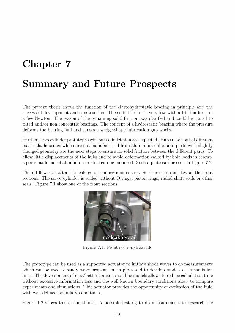
Chapter 7

Summary and Future Prospects

The present thesis shows the function of the elastohydrostatic bearing in principle and thesuccessful development and construction. The solid friction is very low with a friction force ofa few Newton. The reason of the remaining solid friction was clarified and could be traced totilted and/or non concentric bearings. The concept of a hydrostatic bearing where the pressuredeforms the bearing hull and causes a wedge-shape lubrication gap works.

Further servo cylinder prototypes without solid friction are expected. Hubs made out of differentmaterials, housings which are not manufactured from aluminium cubes and parts with slightlychanged geometry are the next steps to ensure no solid friction between the different parts. Toallow little displacements of the hubs and to avoid deformation caused by bolt loads in screws,a plate made out of aluminium or steel can be mounted. Such a plate can be seen in Figure 7.2.

The oil flow rate after the leakage oil connections is zero. So there is no oil flow at the frontsections. The servo cylinder is sealed without O-rings, piston rings, radial shaft seals or otherseals. Figure 7.1 show one of the front sections.

Figure 7.1: Front section/free side

The prototype can be used as a supported actuator to initiate shock waves to do measurementswhich can be used to study wave propagation in pipes and to develop models of transmissionlines. The development of new/better transmission line models allows to reduce calculation timewithout excessive information loss and the well known boundary conditions allow to compareexperiments and simulations. This actuator provides the opportunity of excitation of the fluidwith well defined boundary conditions.

Figure 1.2 shows this circumstance. A possible test rig to do measurements to research the

59

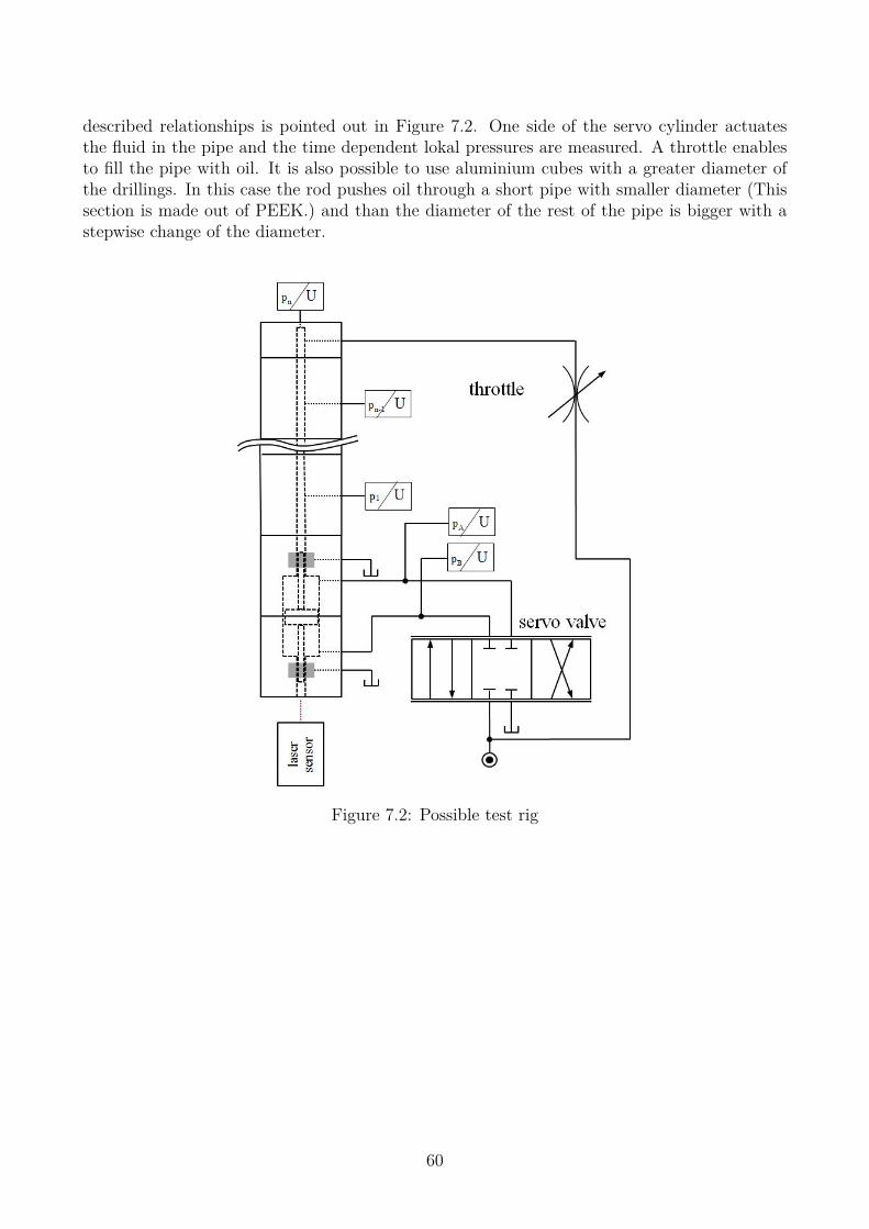
described relationships is pointed out in Figure 7.2. One side of the servo cylinder actuatesthe fluid in the pipe and the time dependent lokal pressures are measured. A throttle enablesto fill the pipe with oil. It is also possible to use aluminium cubes with a greater diameter ofthe drillings. In this case the rod pushes oil through a short pipe with smaller diameter (Thissection is made out of PEEK.) and than the diameter of the rest of the pipe is bigger with astepwise change of the diameter.

Figure 7.2: Possible test rig

60

Bibliography

[1] Buchberger G. Konzepte fur Touchpads, Tastenfelder und positionsempfindli-che Beruhrungssensoren und deren flexible Realisierungen auf Basis von zellularenPolypropylen-Ferroelektreten. Master Thesis p. 1, Johannes Kepler Universitat, 2010.

[2] http://en.wikipedia.org/wiki/Hydraulics. November 2014.

[3] Woodcroft B. The Pneumatics of Hero of Alexandria. Taylor Walton and Maberly, London,1851.

[4] Fries C. and Manhartsgruber B. Cfd based modeling of wave propagation in liquid trans-mission line junctions. Proceedings of ASME 2013 Fluids Engineering Division SummerMeeting, 1A:pp. V01AT03A025, 2013.

[5] Fries C. and Manhartsgruber B. Dynamics of transmission line junctions - comparisonoc cfd results against measurements. Proceedings of 8th FPNI Ph.D Symposium on FluidPower, 1:pp. V001T02A003, 2014.

[6] Buresti G. Elements of Fluid Dynamics. pp. 21-77, Imperial College Press, London, 3edition, 2012.

[7] Scheidl R. Skriptum Olhydraulik. pp. 6/1-6/15, Johannes Kepler Universitat, Linz, 2013.

[8] Will D. and Gebhardt N. Hydraulik - Grundlagen, Komponenten, Schaltungen. pp. 13-41,Springer, Heidelberg, 5 edition, 2011.

[9] http://de.wikipedia.org/wiki/Aluminium. November 2014.

[10] http://en.wikipedia.org/wiki/Thermal expansion. January 2014.

[11] http://de.wikipedia.org/wiki/Baustahl. November 2014.

[12] Ensinger GmbH. Tecapeek natural - Data sheet, October 2014.

[13] http://de.wikipedia.org/wiki/Kupfer. January 2015.

[14] Kokernak R. P. Fluid Power Technology. pp. 32-44, Prentice Hall, Upper Sadle River, 2edition, 1999.

[15] Reynolds O. On the theory of lubrication and its application to mr. beauchamp tower’sexperiments, including an experimental determination of the viscosity of olive oil. Philo-sophical Transactions of the Royal Society of London, 177:pp.157–234, 1886.

[16] Barus C. Isotherms, osipeitics and isometrics relative to viscosity. American Journal ofSciene, 3(45):87–96, 1893.

i

[17] eni. Agip Arnica S - Data sheet, November 2014.

[18] Krieger M. and Gittler P. Thermofluiddynamik. pp. 5-26, Johannes Kepler Universitat,Linz, 2012.

[19] Durst F. Fluid Mechanics. pp. 113-128, Springer, Heidelberg, 1 edition, 2008.

[20] http://en.wikipedia.org/wiki/Derivation of the Navier-Stokes equations. November 2014.

[21] Hamrock B. J., S. R. Schmied, and B. Jacobson. Fundamentals of Machine Elements. pp.480 - 525, McGraw Hill, 2 edition, 2005.

[22] Spurk J.H. Stromungslehre. pp. 210-213, Springer, Heidelberg, 5 edition, 2004.

[23] Collins J. A., Busby H., and Staab G. Mechanical Design of Machine Elements andMachines. pp. 403-428, Jon Wiley and Sons, 2 edition, 2010.

[24] http://en.wikipedia.org/wiki/Plain bearing. November 2014.

[25] http://www.substech.com/dokuwiki/doku.php?id=requirements to engine bearing materials.November 2014.

[26] Decker K. H. Maschinenelemente - Funktion, Gestaltung, Berechnung. pp. 436-456, CarlHanser, 17 edition, 2009.

[27] Murrenhoff H. Servohydraulik. pp. 137 - 146, Institut fur fluidtechnische Antriebe undSteuerungen, Aachen, 1998.

[28] Manhartsgruber B. Skriptum Servohydraulik. pp. 34-40, Johannes Kepler Universitat,Linz, 2011.

[29] Niemann G. Maschinenelemente - Band 1. pp.362 - 365, Springer, Heidelberg, 1981.

[30] http://www.forum-sondermaschinenbau.de/seiten/ausdehungskoeffizient.htm. November2014.

[31] Petrus Blok. Das hydrostatische Keilspaltlager. pp. 1-72, Technische Hogeshool Delft, 1976.

[32] Simulia (Dassault Systemes). Abaqus Theory Guide 6.14 - Chapter 2.5 - Modal dynamics,December 2014.

[33] Simulia (Dassault Systemes). Abaqus Analysis User’s Guide 6.14 - Chapter 26.1.1 - Ma-terial damping, December 2014.

[34] http://www.ibk.ethz.ch/emeritus/da/education/TD/Downloads/TD MMS 2 DAE HS09 DS.pdf. December 2014.

[35] Simulia (Dassault Systemes). Abaqus/CAE User’s Guide 6.14 - Chapter 17.6.1 - Verifyingyour mesh, December 2014.

[36] http://www.cncshop.at/index.php?a=36. January 2015.

[37] http://www.dew-stahl.com/fileadmin/dew-stahl.com/documents/Publikationen/Werkstoffdatenblaetter/Baustahl/1.1213.pdf. January 2015.

ii

[38] Haberle G. Tabellenbuch Mechatronik. pp. 120-121, Europa-Lehrmittel, Haan-Gruiten, 2edition, 2002.

[39] Parker Hannifin GmbH & Co KG. O-Ring Handbook, April 2007.

iii

Acknowledgement

This master thesis was another chance to explore the world of academics, to merge with scienceand to earn wings. It is also the top and the end of five years of studying.

First of all, I would like to express my gratitude and thanks to my advisor and supervisora.Univ.-Prof. Dipl.-Ing Dr. Bernhard Manhartsgruber for his advice, patience and support,while leading my diploma thesis. Furthermore for his useful comments and remarks.

Many thanks also belongs to the head of institute o.Univ.-Prof. Dipl.-Ing. Dr. Rudolf Scheidland all the members of the Institute of Machine Design and Hydraulic Drives. So i could dothe master thesis in a calm and professional atmosphere and achieve the goals set.

Additionally, I want to express my gratitude to Reinhold Wartecker. Without his skills aboutmanufacturing processes a realization would not be possible.

I would like to thank Ing. Siegfried Grammer for his help and advice. His skills and knowledgeabout hydraulics helps me to do measurements without causing a disaster.

Especially, I am grateful to my family, friends and my loved ones for their encouragement,appreciation and patience. Persons, which supported me and contributed valuable time andmoney to my education and they kept my options open.

Many thanks to my colleagues, which dedicated their life to science and technology. We hadto reach the same goals and spent the same time to achieve them. We stood together.

There are so many great scientists and researchers in history, which continue to push backthe boundaries of human knowledge. So my last think is about my conviction: Humans aretechnicians!

iv

Statutory declaration/EidesstattlicheErklarung

Ich erklare an Eides statt, dass ich die vorliegende Masterarbeit selbststandig und ohne fremdeHilfe verfasst, andere als die angegebenen Quellen und Hilfsmittel nicht benutzt bzw. die wort-lich oder sinngemaß entnommenen Stellen als solche kenntlich gemacht habe. Die vorliegendeMasterarbeit ist mit dem elektronisch ubermittelten Textdokument identisch.

Linz, am 16. Februar 2015

Lukas Muttenthaler

v

development of a hydraulic servo cylinder with an

Documents