development of a land surface hydrologic modeling and data
TRANSCRIPT

The Pennsylvania State University
The Graduate School
Department of Meteorology
DEVELOPMENT OF A LAND SURFACE HYDROLOGIC
MODELING AND DATA ASSIMILATION SYSTEM
FOR THE STUDY OF
SUBSURFACE-LAND SURFACE INTERACTION
A Dissertation in
Meteorology
by
Yuning Shi
c© 2012 Yuning Shi
Submitted in Partial Fulfillmentof the Requirements
for the Degree of
Doctor of Philosophy
August 2012

The dissertation of Yuning Shi was read and approved1 by the following:
Kenneth J. DavisProfessor of MeteorologyDissertation AdvisorChair of Committee
Christopher J. DuffyProfessor of Civil Engineering
Fuqing ZhangProfessor of Meteorology
Marcelo ChameckiAssistant Professor of Meteorology
Johannes VerlindeProfessor of MeteorologyAssociate Head of the Department of Meteorology
1Signatures on file in the Graduate School.

iii
Abstract
Coupled models of the land surface and the subsurface, which incorporate hydro-
logic components into LSMs and couple the deeper subsurface with the atmosphere, may
yield significant improvements in both short-term climate forecasting and flood/drought
forecasting. A fully-coupled land surface hydrologic model, Flux-PIHM, is developed by
incorporating a land-surface scheme into the Penn State Integrated Hydrologic Model
(PIHM). The land-surface scheme is mainly adapted from the Noah LSM, which is widely
used in mesoscale atmospheric models and has undergone extensive testing. Because
PIHM is capable of simulating lateral water flow and deep groundwater, Flux-PIHM is
able to represent both the link between groundwater and the surface energy balance as
well as some of the land surface heterogeneities caused by topography.
Flux-PIHM has been implemented at the Shale Hills watershed (0.08 km2) in
central Pennsylvania. Observations of discharge, water table depth, soil moisture, soil
temperature, and sensible and latent heat fluxes in June and July 2009 are used to man-
ually calibrate Flux-PIHM. Model predictions from 1 March to 1 December 2009 are
evaluated. Model predictions of discharge, soil moisture, water table depth, sensible and
latent heat fluxes, and soil temperature show good agreement with observations. The
discharge prediction is comparable to state-of-the-art conceptual models implemented
at similar watersheds. Comparisons of model predictions between Flux-PIHM and the
original hydrologic model PIHM show that the inclusion of the complex surface energy
balance simulation only brings slight improvement in hourly model discharge predictions.
iv
Flux-PIHM does improve the evapotranspiration prediction at hourly scale, the predic-
tion of total annual discharge, and also improves the predictions of some peak discharge
events, especially after extended dry periods. Model results reveal that annual average
sensible and latent heat fluxes are strongly correlated with water table depth, and the
correlation is especially strong for the model grids near the river.
To simplify the procedure of model calibration, a Flux-PHIM data assimilation
system is developed by incorporating the ensemble Kalman filter (EnKF) into Flux-
PIHM. This is the first parameter estimation using EnKF for a physically-based hydro-
logic model. Both synthetic and real data experiments are performed at the Shale Hills
watershed to test the capability of EnKF in parameter estimation. Six model param-
eters selected from a model parameter sensitivity test are estimated. In the synthetic
experiments, synthetic observations of discharge, water table depth, soil moisture, land
surface temperature, sensible and latent heat fluxes, and transpiration are assimilated
into the system. Results show that EnKF is capable of accurately estimating model
parameter values for Flux-PIHM. The estimated parameter values are very close to the
true parameter values. Synthetic experiments are also performed to test the efficiency
of assimilating different observations. It is found that discharge, soil moisture, and land
surface temperature (or sensible and latent heat fluxes) are the most critical observations
for Flux-PIHM calibration. In real data experiments, in situ observations of discharge,
water table depth, soil moisture, and sensible and latent heat fluxes are assimilated.
Results show that, for five out of the six parameters, the EnKF-estimated parameter
values are very close to the manually-calibrated parameter values. The predictions using
EnKF-estimated parameters and manually-calibrated parameters are also similar. Thus

v
the results demonstrate that, given a limited number of site-specific observations, an
automatic sequential calibration method (EnKF) can be used to optimize Flux-PIHM
for watersheds like Shale Hills.

vi
Table of Contents
List of Tables . . . . . . . . . . . . . . . . . . . . . . . . . . . . . . . . . . . . . . viii
List of Figures . . . . . . . . . . . . . . . . . . . . . . . . . . . . . . . . . . . . . ix
Acknowledgments . . . . . . . . . . . . . . . . . . . . . . . . . . . . . . . . . . . xii
Chapter 1. Introduction . . . . . . . . . . . . . . . . . . . . . . . . . . . . . . . . 11.1 Background . . . . . . . . . . . . . . . . . . . . . . . . . . . . . . . . 1
1.1.1 Limitations of land surface models . . . . . . . . . . . . . . . 21.1.2 Limitations of hydrologic models . . . . . . . . . . . . . . . . 111.1.3 Hydrologic model calibration . . . . . . . . . . . . . . . . . . 16
1.2 Objectives . . . . . . . . . . . . . . . . . . . . . . . . . . . . . . . . . 20
Chapter 2. Development of a Coupled Land Surface Hydrologic Model . . . . . 222.1 Introduction . . . . . . . . . . . . . . . . . . . . . . . . . . . . . . . . 222.2 Description of the coupled land surface hydrologic model . . . . . . . 30
2.2.1 The Penn State Integrated Hydrologic Model . . . . . . . . . 302.2.2 The land surface scheme . . . . . . . . . . . . . . . . . . . . . 322.2.3 Fully-coupled land surface hydrologic modeling system . . . . 402.2.4 Test cases . . . . . . . . . . . . . . . . . . . . . . . . . . . . . 42
2.3 Site and data . . . . . . . . . . . . . . . . . . . . . . . . . . . . . . . 422.3.1 The Shale Hills Critical Zone Observatory . . . . . . . . . . . 422.3.2 Model setup and model parameters . . . . . . . . . . . . . . . 442.3.3 Forcing data and evaluation data . . . . . . . . . . . . . . . . 51
2.4 Optimization and evaluation of Flux-PIHM . . . . . . . . . . . . . . 562.4.1 Model optimization and spin-up . . . . . . . . . . . . . . . . 562.4.2 Water budget . . . . . . . . . . . . . . . . . . . . . . . . . . . 612.4.3 Evaluation of hydrologic predictions . . . . . . . . . . . . . . 632.4.4 Evaluation of surface energy balance predictions . . . . . . . 68
2.5 Correlation between surface heat fluxes and water table depth . . . . 712.6 Discussions and conclusions . . . . . . . . . . . . . . . . . . . . . . . 74
Chapter 3. Evaluation of Flux-PIHM Parameter Sensitivities . . . . . . . . . . . 793.1 Introduction . . . . . . . . . . . . . . . . . . . . . . . . . . . . . . . . 793.2 Flux-PIHM Model Parameters . . . . . . . . . . . . . . . . . . . . . 813.3 Experimental Setup . . . . . . . . . . . . . . . . . . . . . . . . . . . 853.4 Results . . . . . . . . . . . . . . . . . . . . . . . . . . . . . . . . . . . 91
3.4.1 Distinguishability . . . . . . . . . . . . . . . . . . . . . . . . . 913.4.2 Observability . . . . . . . . . . . . . . . . . . . . . . . . . . . 1023.4.3 Simplicity . . . . . . . . . . . . . . . . . . . . . . . . . . . . . 109
3.5 Discussions and conclusions . . . . . . . . . . . . . . . . . . . . . . . 112

vii
Chapter 4. Flux-PIHM Parameter Estimation Using Ensemble Kalman Filter: ASynthetic Experiment . . . . . . . . . . . . . . . . . . . . . . . . . . 116
4.1 Introduction . . . . . . . . . . . . . . . . . . . . . . . . . . . . . . . . 1164.2 Development of the Flux-PIHM data assimilation system . . . . . . 123
4.2.1 EnKF . . . . . . . . . . . . . . . . . . . . . . . . . . . . . . . 1234.2.2 Implementation of EnKF in Flux-PIHM . . . . . . . . . . . . 126
4.3 Experimental setup . . . . . . . . . . . . . . . . . . . . . . . . . . . . 1314.4 Results . . . . . . . . . . . . . . . . . . . . . . . . . . . . . . . . . . . 137
4.4.1 Optimal assimilation interval . . . . . . . . . . . . . . . . . . 1374.4.2 Capability of EnKF . . . . . . . . . . . . . . . . . . . . . . . 1394.4.3 Efficiency of assimilating different observations . . . . . . . . 1424.4.4 Parameter interaction . . . . . . . . . . . . . . . . . . . . . . 152
4.5 Discussions and conclusions . . . . . . . . . . . . . . . . . . . . . . . 153
Chapter 5. Flux-PIHM Parameter Estimation Using Ensemble Kalman Filter: AReal-Data Experiment . . . . . . . . . . . . . . . . . . . . . . . . . . 157
5.1 Introduction . . . . . . . . . . . . . . . . . . . . . . . . . . . . . . . . 1575.2 Preprocessing of observations . . . . . . . . . . . . . . . . . . . . . . 1605.3 Experimental setup . . . . . . . . . . . . . . . . . . . . . . . . . . . . 1655.4 Results . . . . . . . . . . . . . . . . . . . . . . . . . . . . . . . . . . . 1675.5 Discussions and conclusions . . . . . . . . . . . . . . . . . . . . . . . 173
Chapter 6. Summary . . . . . . . . . . . . . . . . . . . . . . . . . . . . . . . . . 1766.1 Coupled land surface hydrologic model . . . . . . . . . . . . . . . . . 1776.2 Flux-PIHM parameter estimation using the ensemble Kalman filter . 1786.3 Land surface subsurface interaction . . . . . . . . . . . . . . . . . . . 1816.4 Limitation and future work . . . . . . . . . . . . . . . . . . . . . . . 183
Bibliography . . . . . . . . . . . . . . . . . . . . . . . . . . . . . . . . . . . . . . 186

viii
List of Tables
2.1 Soil parameters used for the Shale Hills watershed domain. . . . . . . . 482.2 Parameters used for the river segments. . . . . . . . . . . . . . . . . . . 492.3 Vegetation parameters used for the Shale Hills watershed domain. . . . 502.4 Forcing data used for simulation. . . . . . . . . . . . . . . . . . . . . . . 522.5 Evaluation data used for model optimization and evaluation. . . . . . . 562.6 Calibration coefficient values optimized for Flux-PIHM at the Shale Hills
watershed model domain. . . . . . . . . . . . . . . . . . . . . . . . . . . 602.7 Total bias, NSE, and correlation coefficient of SWAT2005 daily discharge
predictions at six small watersheds in central Texas compared with ob-servations. . . . . . . . . . . . . . . . . . . . . . . . . . . . . . . . . . . . 64
2.8 Bias, NSE, and correlation coefficient of Flux-PIHM and PIHM V2 hourlydischarge predictions compared with RTHnet measurements. . . . . . . 66
2.9 Bias, RMSE and correlation coefficient of Flux-PIHM and PIHM V2hourly WTD and SMC predictions compared with RTHnet well mea-surements. . . . . . . . . . . . . . . . . . . . . . . . . . . . . . . . . . . . 68
2.10 RMSE and correlation coefficient of Flux-PIHM and PIHM V2 hourly Hand LE predictions compared with eddy covariance flux tower measure-ments for different seasons. . . . . . . . . . . . . . . . . . . . . . . . . . 70
3.1 Flux-PIHM model parameters for the sensitivity tests and the plausibleranges of their calibration coefficients. . . . . . . . . . . . . . . . . . . . 86
4.1 Model variables included in the joint Flux-PIHM state-parameter vector. 1274.2 Standard deviation of Gaussian white noise added to each observation
data set. . . . . . . . . . . . . . . . . . . . . . . . . . . . . . . . . . . . . 1324.3 Initial ensemble mean of parameters, assimilation intervals, and assimi-
lated observations of different test cases. . . . . . . . . . . . . . . . . . . 1344.4 Estimated parameter calibration coefficients from different test cases. . . 148
5.1 Errors in the observations when assimilated into the system in the real-data experiment. . . . . . . . . . . . . . . . . . . . . . . . . . . . . . . . 167
5.2 Estimated parameter calibration coefficients from the real-data experiment. 169

ix
List of Figures
1.1 A schematic showing how precipitation deficiencies during a hypothetical4-year period are translated in delayed fashion, over time, through othercomponents of the hydrologic cycle. . . . . . . . . . . . . . . . . . . . . . 4
2.1 Coupling between the hydrologic model (PIHM) and the land surface en-ergy balance model (adapted from the Noah LSM) yielding the integratedmodel, Flux-PIHM. . . . . . . . . . . . . . . . . . . . . . . . . . . . . . . 41
2.2 Map of the Shale Hills watershed. . . . . . . . . . . . . . . . . . . . . . . 432.3 Grid setting for the Shale Hills watershed model domain. . . . . . . . . 452.4 The vegetation type, soil type, surface elevation, and bedrock depth de-
fined in Flux-PIHM for the simulated domain. . . . . . . . . . . . . . . . 462.5 MODIS LAI, SSHO field-measured LAI, and modified MODIS LAI from
2009 to 2010. . . . . . . . . . . . . . . . . . . . . . . . . . . . . . . . . . 532.6 Workflow for manual calibration of Flux-PIHM. . . . . . . . . . . . . . . 582.7 Comparison of water budget between Flux-PIHM and PIHM V2. . . . . 622.8 Comparison of hourly outlet discharge among RTHnet measurements,
Flux-PIHM, and, PIHM V2 predictions. . . . . . . . . . . . . . . . . . . 652.9 Comparison of hourly water table depth and soil water content among
RTHnet wells, Flux-PIHM prediction, and PIHM V2 prediction. . . . . 672.10 Comparison of surface heat fluxes among Flux-PIHM, PIHM V2 and
RTHnet measurements as averaged daily cycles at each hour of the dayfor different seasons. . . . . . . . . . . . . . . . . . . . . . . . . . . . . . 70
2.11 Comparison of hourly soil temperature at 5 cm below surface betweenFlux-PIHM predictions and RTHnet observations . . . . . . . . . . . . . 72
2.12 Annual average sensible and latent heat fluxes plotted as functions ofwater table depth from Flux-PIHM simulation. . . . . . . . . . . . . . . 73
3.1 Correlation coefficients between 20 potentially identifiable Flux-PIHMparameters and modeled hourly outlet discharge from the multi-parametertest. . . . . . . . . . . . . . . . . . . . . . . . . . . . . . . . . . . . . . . 91
3.2 Correlation coefficients between 20 potentially identifiable Flux-PIHMparameters and modeled hourly water table depth at RTHnet wells fromthe multi-parameter test. . . . . . . . . . . . . . . . . . . . . . . . . . . 92
3.3 Correlation coefficients between 20 potentially identifiable Flux-PIHMparameters and modeled hourly soil water content at RTHnet wells fromthe multi-parameter test. . . . . . . . . . . . . . . . . . . . . . . . . . . 92
3.4 Correlation coefficients between 20 potentially identifiable Flux-PIHMparameters and modeled mid-day skin temperature from the multi-parametertest. . . . . . . . . . . . . . . . . . . . . . . . . . . . . . . . . . . . . . . 93

x
3.5 Correlation coefficients between 20 potentially identifiable Flux-PIHMparameters and modeled mid-day sensible heat flux from the multi-parametertest. . . . . . . . . . . . . . . . . . . . . . . . . . . . . . . . . . . . . . . 93
3.6 Correlation coefficients between 20 potentially identifiable Flux-PIHMparameters and modeled mid-day latent heat flux from the multi-parametertest. . . . . . . . . . . . . . . . . . . . . . . . . . . . . . . . . . . . . . . 94
3.7 Correlation coefficients between 20 potentially identifiable Flux-PIHMparameters and modeled mid-day transpiration from the multi-parametertest. . . . . . . . . . . . . . . . . . . . . . . . . . . . . . . . . . . . . . . 94
3.8 Sensitivity of soil water retention curve to α and β values. . . . . . . . . 963.9 RMSC between twenty potentially identifiable Flux-PIHM parameters
and different observable variables. . . . . . . . . . . . . . . . . . . . . . . 1003.10 RMSDs of discharge simulations in single parameter tests. . . . . . . . . 1023.11 RMSDs of WTD simulations in single parameter tests. . . . . . . . . . . 1033.12 RMSDs of SWC simulations in single parameter tests. . . . . . . . . . . 1043.13 RMSDs of mid-day (1700 UTC) Tsfc simulations in single parameter tests. 1043.14 RMSDs of mid-day (1700 UTC) H simulations in single parameter tests. 1053.15 RMSDs of mid-day (1700 UTC) LE simulations in single parameter tests. 1053.16 RMSDs of mid-day (1700 UTC) Et simulations in single parameter tests. 1063.17 Flux-PIHM observable variables at 1700 UTC 20 June 2009 plotted as
functions of model parameters. . . . . . . . . . . . . . . . . . . . . . . . 1103.18 Flux-PIHM observable variables at 1700 UTC 11 July 2009 plotted as
functions of model parameters. . . . . . . . . . . . . . . . . . . . . . . . 111
4.1 Schematic description of EnKF parameter update. . . . . . . . . . . . . 1234.2 Flowchart of Flux-PIHM data assimilation framework for parameter es-
timation. . . . . . . . . . . . . . . . . . . . . . . . . . . . . . . . . . . . 1304.3 True values and temporal evolution of parameters from the test cases
CR, 72 hrs, 48 hrs, and 24 hrs. . . . . . . . . . . . . . . . . . . . . . . . 1384.4 RMSEs of the estimated parameter values over the entire simulation period. 1404.5 True values and temporal evolution of parameters from test cases CR,
Case +, and Case −. . . . . . . . . . . . . . . . . . . . . . . . . . . . . . 1414.6 Evaluation of the hydrologic variable forecasts using the estimated pa-
rameter sets from the test cases CR, Case +, Case −, and NoPE. . . . . 1434.7 Evaluation of the land surface variable forecasts using the estimated pa-
rameter sets from test cases CR, Case +, Case −, and NoPE. . . . . . . 1444.8 True values and temporal evolution of the estimated parameters from
test cases CR, Q, SSHO, and NoSM, NoWTD, and QST. . . . . . . . . 1454.9 Evaluation of the the hydrologic variable forecasts using the estimated
parameter sets from the test cases CR, Q, SSHO, NoSM, NoWTD, QST,and NoPE. . . . . . . . . . . . . . . . . . . . . . . . . . . . . . . . . . . 146
4.10 Evaluation of the land surface variable forecasts using the estimated pa-rameter sets from the test cases CR, Q, SSHO, NoSM, NoWTD, QST,and NoPE. . . . . . . . . . . . . . . . . . . . . . . . . . . . . . . . . . . 147

xi
4.11 Scatterplot of α and β values from all ensemble members from 0000 UTC1 July to 0000 UTC 1 August 2009. . . . . . . . . . . . . . . . . . . . . 152
4.12 Scatterplot of α and β values from all ensemble members from 0000 UTC1 July to 0000 UTC 1 August 2009. . . . . . . . . . . . . . . . . . . . . 154
5.1 Rating curve for SSHO V-notch weir. . . . . . . . . . . . . . . . . . . . . 1615.2 Average error for rating curves with 1 mm error in measured water level. 1635.3 Temporal evolution of estimated parameters in real-data experiment. . . 1685.4 Comparison of discharge predictions between Flux-PIHM run with EnKF-
estimated parameters, Flux-PIHM run with manually calibrated param-eters, and observations from RTHnet. . . . . . . . . . . . . . . . . . . . 170
5.5 Comparison of WTD predictions between Flux-PIHM run with EnKF-estimated parameters, Flux-PIHM run with manually calibrated param-eters, and observations from RTHnet. . . . . . . . . . . . . . . . . . . . 171
5.6 Comparison of SWC predictions between Flux-PIHM run with EnKF-estimated parameters, Flux-PIHM run with manually calibrated param-eters, and observations from RTHnet. . . . . . . . . . . . . . . . . . . . 172
5.7 Comparison of sensible heat flux predictions between Flux-PIHM runwith EnKF-estimated parameters, Flux-PIHM run with manually cali-brated parameters, and observations from RTHnet, plotted as averageddaily cycles. . . . . . . . . . . . . . . . . . . . . . . . . . . . . . . . . . . 172
5.8 Comparison of latent heat flux predictions between Flux-PIHM run withEnKF-estimated parameters, Flux-PIHM run with manually calibratedparameters, and observations from RTHnet, plotted as averaged dailycycles. . . . . . . . . . . . . . . . . . . . . . . . . . . . . . . . . . . . . . 173

xii
Acknowledgments
I gratefully acknowledge my advisor, Dr. Kenneth Davis, for his insightful guid-
ance and encouragement during the past five years. I am also grateful to Dr. Christopher
Duffy, for his help on hydrology, to Dr. Fuqing Zhang, for his help on EnKF, and to Dr.
Marcelo Chamecki.
I want to thank my colleagues from Dr. Davis’ group and from Dr. Duffy’s
group, who are also friends of mine. Working together with them makes research more
enjoyable. I am especially thankful to Xuan Yu who has provided generous help on the
most tedious part.
I want to thank the CZO community at Penn State, especially Dr. Henry Lin,
Dr. David Eissenstat, and Dr. Kusum Naithani, who have provided valuable help with
my research. Without the interdisciplinary cooperation at CZO, this research project
would be impossible.
I would like to thank all my friends, both here and in China, for their support
and encouragement.
I am very grateful to my parents, for helping me become who I am. Especially, I
want to thak my wife, Haiyan. Thank you for being there for the past five years of my
doctoral program, and for the past nine years since I first met you.

xiii
Essentially, all models are wrong, but some are
useful.
—George E. P. Box

1
Chapter 1
Introduction
1.1 Background
The predictability of the atmosphere is limited by the chaotic nature of atmo-
spheric turbulence to a time span of the order of one week or less (Lorenz 1969; Smagorin-
sky 1969; Lorenz 1982). The Earth’s surface, however, has “memories” much longer than
those of the atmosphere. Significant improvements in short-term climate forecasts as well
as weather forecasts can be found by including the modeling of Earth surface, e.g., land
surface processes and sea surface temperature (SST), in predictive models (Palmer and
Anderson 1994; Beljaars et al. 1996; Koster et al. 2000; Goddard et al. 2001; Ek et al.
2003; Mitchell et al. 2004; Kumar et al. 2008). While covering only 30% of Earth’s
surface, the land surface plays a distinctive role in weather and climate because of its
considerable heterogeneity, its dynamic hydrologic cycle and strong variations of tem-
perature, and highly changeable land use and land cover (Yang 2004). Land surface
processes are critical in the growth of atmospheric boundary layer (ABL), the formation
of clouds and precipitation, and the budgets of heat, momentum, and moisture within
the atmosphere. Weather and climate models currently rely on land surface models
(LSMs) to represent land surface processes. LSMs provide lower boundary conditions
and initialize ground state for numerical weather prediction (NWP; Ookouchi et al. 1984;

2
Liang et al. 1994; Betts et al. 1997; Chen et al. 1997a; Xiu and Pleim 2001; Ek et al.
2003; Kumar et al. 2006; Chen et al. 2007; Niu et al. 2011).
Accurate description of land surface memories depends on accurate simulations
of subsurface water dynamics. LSMs, however, always have simplified descriptions of
subsurface hydrology, which limit the ability of LSMs in representing the memories of
land surface. In contrast, hydrologic models tend to have simplified representation of
evapotranspiration, which may affect the accuracy of flood/drought forecasting. Coupled
models of land surface and subsurface, which incorporate hydrologic components into
LSMs or couple deeper subsurface with the atmosphere, may yield improvements in
weather and short-term climate forecasting and flood/drought forecasting.
One obstacle to effective applications of land surface hydrologic models is the
parameter uncertainty. Hydrologic model parameters need to be calibrated for the model
system to reproduce observed hydrologic responses (Moradkhani and Sorooshian 2008).
While many automatic calibration methods have been developed in the past few decades,
manual calibration is still the prevalent choice for physically-based hydrologic models,
due to the high computational cost of such models. This labor-intensive and time-
consuming calibration procedure poses extra difficulty for applying physically-based land
surface hydrologic models.
1.1.1 Limitations of land surface models
The land surface plays an important role in weather and climate. It interacts with
the atmosphere through land surface processes, i.e., the exchange of mass, momentum
and energy between the atmosphere and the land surface. Observational studies found

3
that land surface heterogeneity, e.g., spatial variability in soil moisture, albedo, and
landcover, has strong impact on ABL structure (e.g., LeMone et al. 2002, 2007; Kang
et al. 2007). Model studies found that land surface has strong influences in cloud and
precipitation formations (e.g., Beljaars et al. 1996; Betts et al. 1997; Chen et al. 1997a).
The land surface not only influences concurrent ABL growth, precipitation, and
temperature through the exchange of heat and moisture, but also influences future at-
mospheric circulations by providing memories of atmospheric anomalies. Atmospheric
anomalies, e.g., heavy rainfalls or severe droughts, could cause anomalies in the subsur-
face. As described in Fig. 1.1, the translation of the anomalies to other components of
hydrologic cycles and the dissipation of the anomalies through evapotranspiration take
weeks to months (Changnon 1987; Koster and Suarez 2001). Because land surface could
“remember” the atmospheric anomalies, it would give feedback to future atmospheric
circulations through land surface processes. Although memories of the atmosphere are
limited by its chaotic nature, the memories of the land surface would provide impor-
tant knowledge to short-term climate forecasting. Studies show that the realistic ini-
tialization of land surface states could improve precipitation forecasts at subseasonal
timescales (Koster et al. 2004a), while foreknowledge of land surface moisture state
could significantly improve the predictability of precipitation at seasonal-to-interannual
timescales (Koster et al. 2000). Therefore, providing realistic land surface states to at-
mospheric models is identified as the key to improving weather and seasonal forecasting
skills (Mitchell et al. 2004; Koster et al. 2004a; Chen et al. 2007).
Among all land surface variables, soil moisture is probably the most essential. Soil
moisture determines the partitioning of available energy into sensible, latent and ground

4
Fig. 1.1. A schematic showing how precipitation deficiencies during a hypothetical 4-
year period are translated in delayed fashion, over time, through other components of
the hydrologic cycle. Source: Figure 2 from Changnon (1987).
5
heat fluxes, as well as the partitioning of incoming precipitation into surface runoff and
infiltration. Soil moisture acts as a source of water for the atmosphere. Strong coupling
between soil moisture and precipitation has been found (Koster et al. 2004b). The
transport of soil water content affects the heat transport with in the soil column and
at the land surface. The memory effect of the land surface mostly relies on the lagged
response of soil moisture to precipitation and drought anomalies.
Including land surface states into atmospheric models is much more difficult than
the inclusion of SST (Betts et al. 1996). SST has small spatial variability and high fre-
quency observations. Land surface, however, has considerable heterogeneity and highly
changeable land use and land cover. The current observation network is insufficient to
monitor the changes in land surface states at small temporal and spatial scales (Yang
2004; Betts et al. 1996). Land surface states therefore must be obtained by numeri-
cal simulations. LSMs are the numerical models that simulate land surface processes.
LSMs provide necessary physical boundary conditions for atmospheric models, including
surface sensible and latent heat fluxes, upward longwave radiation (or surface skin tem-
perature and surface emissivity), and upward shortwave radiation (or surface albedo).
The initialization of land surface states in atmospheric models also relies on LSMs.
Although land surface processes are important for atmospheric modeling, those
processes were not included in the early general circulation models (GCMs) before the
late 1960s. Surface temperature was either prescribed in GCMs, or solved using a simple
energy balance equation based on time-fixed soil moisture. Manabe (1969) introduced
the “bucket model” into GCMs with the ability to simulate time and space varying soil
moisture. In the bucket model, global soil is represented by 15 cm deep “buckets”. The

6
rate of change of soil moisture is equal to the difference between the rate of rainfall and
the rate of evapotranspiration. When the bucket is full, the excess precipitation becomes
surface runoff. Evapotranspiration is regulated by soil moisture content. However crude
it is, the bucket model is the first attempt to account for memories of soil moisture in
atmospheric models.
The so-called “big-leaf model” proposed by Deardorff (1978) is a milestone in
LSM development. A single layer of vegetation is included in the model which explic-
itly represents canopy interception, canopy evaporation, and canopy transpiration. The
inclusion of vegetation layer provides possibilities for future advanced LSM development.
In the past three decades, many advanced LSMs have been developed. Sophisti-
cated hydrological, biophysical, biochemical, and ecological processes have been included
into LSMs. Some advanced LSMs have been implemented in operational NWP models
and have provided improved forecast results (Ek et al. 2003; Mitchell et al. 2004; Kumar
et al. 2008). The evolution of LSMs from the bucket model to advanced LSMs reflects
the community’s effort to improve the representation of land surface fluxes, including
the benefit of capturing the memory embedded in subsurface (Ek et al. 2003; Mitchell
et al. 2004).
In most LSMs, however, hydrological processes are not well described. LSMs can
be regarded as one-dimensional grid models (Yang 2004). Most of modern LSMs have
soil columns with depths of 1–2 m and divided into multiple layers. Vertical flow of soil
water content is described using the Richards equation while the horizontal transport
of water is ignored. Most LSMs even neglect deeper soil moisture processes and lack
physical representation of water table. The complexity of runoff formulation, at both

7
surface and subsurface, is relatively low. For example, the Noah LSM (Chen and Dudhia
2001; Ek et al. 2003), the Pleim-Xiu LSM (Xiu and Pleim 2001), the Rapid Update
Cycle (RUC; Smirnova et al. 1997) LSM, the Simplified Simple Biosphere model (SSiB;
Xue et al. 1991), and the Noah LSM with multiparameterization options (Noah-MP;
Niu et al. 2011) are the LSM options embedded in the Advanced Research Weather
Research and Forecasting (WRF) Modeling System Version 3.4. Those LSMs have two
to nine soil layers with total depths between 0.8 to 2 m. All of those LSMs, except for
Noah-MP, have no explicit representation of groundwater. In the Noah LSM and SSiB,
subsurface runoff is parameterized by a gravitational percolation term (Chen and Dudhia
2001), which is a linear function of bottom soil layer drainage affected by soil type, soil
moisture content, and slope; surface runoff is described with a simple infiltration-excess
scheme. In the Pleim-Xiu LSM, soil column is more “bucket like”, with runoff occurring
when soil moisture excesses saturation. Noah-MP has an additional aquifer layer below
the standard 2 m soil column and a physical representation of the water table. But the
model has no description of the layer between the bottom of soil layer and the water
table. The subsurface runoff in Noah-MP is also highly parameterized. None of those
models take account of the horizontal flow of groundwater.
Runoff predictions of LSMs are far from satisfactory (Wood et al. 1998; Lohmann
et al. 1998; Gedney et al. 2000; Lohmann et al. 2004; Boone et al. 2004; Rosero et al.
2011). The evaluation of runoff predictions of LSMs has been the focus of many projects,
e.g., the Project for Intercomparison of Land-surface Parameterization Schemes (PILPS)
Phase 2(c) (Wood et al. 1998; Lohmann et al. 1998), PILPS Phase 2(e) (Bowling et al.

8
2003; Nijssen et al. 2003), the multi-institutional North American Land Data Assim-
ilation System Project (NLDAS; Mitchell et al. 2004; Lohmann et al. 2004), and the
Rhone-Aggregation Land Surface Scheme Intercomparison Project (Rhone-AGG; Boone
et al. 2004). Results show that the intermodel differences of mean annual runoff have the
same magnitude as the mean observed runoff (Lohmann et al. 1998; Nijssen et al. 2003;
Lohmann et al. 2004; Boone et al. 2004). The partitioning of runoff into surface and
subsurface runoff, and the spatial distribution of runoff are also quite different from one
scheme to another (Lohmann et al. 1998, 2004; Boone et al. 2004). Predictions of runoff
in summer season and in arid areas are extremely difficult for most of the evaluated
LSMs as they tend to overestimate low flows (Lohmann et al. 1998). Lohmann et al.
(2004) concluded that “we cannot model streamflow in most basins within the United
States without more work done”. At short time scale, the errors in runoff prediction
would degrade the soil moisture prediction by providing inaccurate boundary conditions
for soil moisture transport, and in turn degrade evapotranspiration predictions (Liang
et al. 2003; Chen and Hu 2004; Lohmann et al. 2004). At long time scale, from the water
balance perspective, an underestimation (overestimation) of total runoff would cause an
overestimation (underestimation) of total evapotranspiration (Wood et al. 1998; Liang
et al. 1998; Lohmann et al. 1998; Nijssen et al. 2003; Lohmann et al. 2004; Boone et al.
2004).
Groundwater is another important reservoir. Groundwater interacts with soil
water via recharge and capillary effects. The water flux between groundwater and soil
column acts as the lower boundary condition for soil moisture transport. The location

9
of water table affects soil moisture profile, which in turn affects the rate of evapotran-
spiration. The lateral groundwater flow affects the spatial pattern of soil moisture and
evapotranspiration as well. Liang et al. (2003) added explicit modeling of water table and
groundwater atmosphere interaction into the three-layer Variable Infiltration Capacity
model (VIC-3L). Comparison between the new model (referred to as VIC-ground) and
VIC-3L demonstrates that the deeper soil layer in the VIC-ground is generally wetter
than that in VIC-3L, while the top soil layers in VIC-ground are generally drier than
in VIC-3L. The differences in soil moisture profile result in lower surface runoff, higher
base flow, and lower evapotranspiration in VIC-ground than in VIC-3L. Chen and Hu
(2004) found that the soil moisture content in a soil hydrological model with groundwater
component could be notably higher than the model without groundwater component.
In their case, the model with groundwater component shows higher evapotranspiration
rate. The inclusion of groundwater component also changes the spatial distribution of
soil moisture content.
Groundwater dynamics have strong interactions with surface heat fluxes (Maxwell
et al. 2007; Kollet and Maxwell 2008; Rihani et al. 2010). Implementing an integrated
land surface groundwater model at the Little Washita watershed, Oklahoma, Kollet and
Maxwell (2008) found that surface heat fluxes can be correlated with water table as
deep as 5 m. When water table is close to land surface, groundwater could directly
provide water for evapotranspiration (NRC 2004). Those studies imply the significance
of including groundwater modeling for accurate soil moisture content simulations and
accurate surface energy balance simulations.

10
Furthermore, groundwater also has lagged response to atmospheric anomalies due
to the interaction with soil water. The memory of groundwater can be even longer than
soil moisture (Changnon 1987; Dooge 1992; Skøien et al. 2003). Because of the lack of
groundwater dynamics, LSMs have limited ability in representing the spatial heterogene-
ity of soil moisture and the contribution of groundwater to land surface memories.
There has been recent interest in incorporating a hydrologic component into LSMs
or coupling deeper subsurface with the atmosphere to improve the representation of soil
moisture at the land surface (e.g., York et al. 2002; Seuffert et al. 2002; Molders and
Ruhaak 2002; Liang et al. 2003; Yeh and Eltahir 2005; Maxwell and Miller 2005; Gulden
et al. 2007; Maxwell et al. 2007; Kollet and Maxwell 2008; Rosero et al. 2011). York
et al. (2002) coupled a single column vertically discretized atmospheric model with a dis-
tributed soil-vegetation-aquifer model to study groundwater-atmosphere interactions at
a small northeastern Kansas catchment on decadal timescales. The coupled model is able
to capture monthly and yearly trends in precipitation, runoff, and evapotranspiration.
Results reveal that 5%–20% of annual evapotranspiration is drawn from groundwater. A
40 year extended drought condition simulation shows that the response time of groundwa-
ter to the drought condition is on the order of 200 years, which proves that groundwater
has a long memory of atmospheric anomalies. Seuffert et al. (2002) linked a simple land-
surface hydrologic model with an atmospheric model using a two-way coupling strategy.
By including more realistic simulation of surface and subsurface conditions, the coupled
model provides improved predictions of surface heat fluxes and precipitations compared
with the stand-alone atmospheric model. Molders and Ruhaak (2002) coupled a surface

11
and channel runoff model to an atmospheric model to study the effect of runoff pre-
dictions on atmospheric predictions. The models with and without runoff model show
notable differences in cloud formation and precipitation. The inclusion of runoff model
also improves the prediction of landcover change impacts. Maxwell and Miller (2005),
Maxwell et al. (2007), Kollet and Maxwell (2006; 2008), and Rihani et al. (2010) have
incorporated a fully-coupled, three-dimensional (subsurface and overland) groundwater
flow model with different land surface models and mesoscale atmospheric models to study
the influences of lateral subsurface water flow and shallow water table depth on surface
energy balances. Results indicate that coupled land surface groundwater models be-
have differently from uncoupled land surface models in synthetic data experiments, and
reveal strong correlation between land surface and subsurface. The improvement of cou-
pled model in flood/drought forecasting and surface heat flux prediction over uncoupled
models has yet to be examined. The interactions between land surface and subsurface
for different topography, soil type, and landcover also need further exploration.
1.1.2 Limitations of hydrologic models
The water cycle, or hydrologic cycle is central to the Earth system, and water re-
sources are one of the critical environmental and political issues of the 21st century (NRC
2004). A primary goal of contemporary water cycle research is to significantly improve
the understanding of water cycle processes, and to incorporate this understanding into
prediction frameworks that can be used for decision making (Hornberger et al. 2001).
Hydrologic models are important tools to enhance the understanding of hydrological
processes and to simulate and predict hydrological events for better decision making.

12
Hydrologic models are designed to answer the question, “what happens to the
rain” (Penman 1961). The earliest hydrologic model to answer this question is the ratio-
nal formula developed by Mulvany (1851). It statistically relates storm runoff rates to
rainfall intensity and watershed area using regression method. More empirical rainfall-
runoff (R-R) models were then developed (e.g., Sherman 1932; Horton 1935). Empirical
models describe the relation between rainfall and runoff mathematically with little con-
sideration of physical processes. These models need a lot of historical precipitation and
runoff data to establish the mathematical relationship.
In 1960s, more components of the water cycle were added to hydrologic mod-
els with the introduction of digital computer. Limited by hydrologic data availability
and computer power at that time, those hydrological processes were conceptually and
parametrically represented. Examples of early conceptual R-R models are the Stanford
Watershed Model (SWM; Linsley and Crawford 1960; Crawford and Linsley 1966), the
Catchment Model (CM; Dawdy and O’Donnell 1965), and the Tank Model (Sugawara
1967). Because of their simple model structures, efficient computational cost, and their
success in flood forecasting, more conceptual models, both lumped and distributed, have
been developed. Today, many of them are still widely used (Kampf 2006; Wood and
Lettenmaier 2006), e.g., the Soil Water Assessment Tool (SWAT; Arnold et al. 1998),
the Soil-Vegetation-Atmosphere Transfer model (SVAT; Ma and Cheng 1998), and the
Sacramento Soil Moisture Accounting model (SAC-SMA; Burnash et al. 1973; Burnash
1995) which is used for the National Weather Service (NWS) river forecast.
Conceptual models, however, provide little help in enhancing our knowledge and
understanding of hydrological processes. Conceptual models are highly simplified and

13
parameterized representations of hydrological processes. Storage units (e.g., surface wa-
ter, saturated water and unsaturated water) are described as non-linear reservoirs. Most
of the parameters used in those models are purely optimal numbers which could pro-
vide best model predictions, but lack physical meanings, and can only be obtained by
model calibration. Like empirical models, the calibration of conceptual models requires
sufficiently long records of meteorological conditions and watershed responses, which are
always not available especially for small-scale, low-order watersheds. The obtained con-
ceptual model calibration coefficients at one scale or at one watershed are hardly able
to be transferred to another scale or another watershed (Bergstrom and Graham 1998;
Reed et al. 2004).
To link model parameter values with physical meanings, and to physically de-
scribe hydrological processes, physically-based models were developed to overcome those
deficiencies of conceptual models. Examples of this type of models are the Systeme
Hydrologique Europeen (SHE; Abbott et al. 1986a,b), the Physically Based Runoff Pro-
duction Model (TOPMODEL; Beven and Kirkby 1976, 1979), the Institute of Hydrology
Distributed Model (IHDM; Beven et al. 1987), the THALES model (Grayson et al. 1992),
the Distributed Hydrological Model (HYDROTEL; Fortin et al. 2001a,b), and the Penn
State Integrated Hydrologic Model (PIHM; Qu 2004; Qu and Duffy 2007; Kumar 2009).
Physically-based spatially-distributed hydrologic models take into account spatial
heterogeneity of inputs, and have the capability of characterizing hydrologic variables
in space (Beven 1985; Smith et al. 2004; Wood and Lettenmaier 2006; Li et al. 2009).
They can also be applied to those watersheds where no adequate data are available for

14
calibrating empirical and conceptual models (Beven 1985; Smith et al. 2004). Physically-
based hydrologic models are therefore extremely important for forecasting at small-scale,
low-order watersheds and for the study and understanding of hydrological processes.
While more and more complex physics such as horizontal subsurface flow, macrop-
ore flow, coupled surface water flow, and 3-D subsurface are included in physically-based
models, those models usually have simplified representations of evapotranspiration and
other land surface processes. In many hydrologic models, potential evapotranspiration is
not calculated, and has to be specified as atmospheric forcing. Examples of such models
are the WASH123D model (Yeh et al. 2006), IHDM (Beven et al. 1987), the Kinematic
Runoff and Erosion model (KINEROS; Woolhiser et al. 1990; Smith et al. 1995), and
THALES (Grayson et al. 1992), to name a few (Kampf and Burges 2007). The accuracy
of evapotranspiration calculation is then limited by the quality of off-line potential evap-
otranspiration calculation and the grid compatibility between model and forcing data.
For those models that calculate potential evapotranspiration, some of them use simple
empirical equations (e.g., Thornthwaite 1948; Hamon 1963; Turc 1961; Jensen and Haise
1963; Hargreaves et al. 1985) in order to reduce the requirement of forcing data. Most
of those equations only take account of air temperature and solar radiation input. The
most widely used potential evapotranspiration formulations are the Priestley and Taylor
(1972) equation and the Penman-Monteith (Monteith 1965) equation. In the Priestley
and Taylor equation, potential latent heat flux LEp is formulated as
LEp = αPT∆
∆ + γ(Rn − G) , (1.1)

15
where αPT is the empirical Priestley-Taylor number, ∆ is the rate of change of saturation
specific humidity with air temperature, γ is the psychrometric constant, Rn is the net
radiation, and G is the ground heat flux. In Penman-Monteith equation,
LEp =∆ (Rn − G) + ρacp (es − ea) /ra
∆ + γ (1 + rs/ra), (1.2)
where ρa is the air density, cp is the specific heat of air, es is the saturated vapor pressure,
ea is the actual vapor pressure, rs is the canopy resistance, and ra is the aerodynamic
resistance. Due to the lack of land surface process formulations, the estimation of net
radiation, ground heat flux, and ra tend to be crude and highly empirical in hydrologic
models. In some hydrologic models, land surface radiation and energy fluxes are deduced
from watershed location, season, topography, and vegetation (Kampf and Burges 2007).
Ground heat flux G is often estimated as a fixed fraction of Rn, and ra is simplified
as a function of wind speed. Some models also ignore the temporal variation of rs.
The differences between potential evapotranspiration formulations have been the focus
of many studies (e.g., Vorosmarty et al. 1998; Kampf 2006; Weiß and Menzel 2008).
Results show that different methods can produce significantly different estimations in
evapotranspiration. Total evapotranspiration calculated using different methods could
differ by hundreds of millimeters per year, and the differences are even larger in hot and
dry areas (Vorosmarty et al. 1998). The calculation of actual evaporation adds more
uncertainties to hydrologic models predictions.
Evapotranspiration is an important component of water cycle and an important
process in hydrologic models. Globally, over 60% of precipitation over land surface goes

16
back to the atmosphere in the form of evapotranspiration (Lvovitch 1970). The exchange
of water and energy between land surface and atmosphere considerably influences hy-
drologic characteristics (Kavvas et al. 1998; Singh and Woolhiser 2002). At short time
scales, accurate forecasting of timing and magnitude of peak discharge depends on the
accurate forecast of evapotranspiration, especially after extended dry periods (Kampf
2006). At long time scales, the total incoming precipitation is about the sum of total
runoff and total evapotranspiration. Errors in total evapotranspiration simulation impair
the accuracy of total runoff. Moreover, idealized simulations of groundwater land surface
interaction reveal strong correlations between land surface fluxes and water table depth
(Rihani et al. 2010). The results suggest that spatial heterogeneities in landform and to-
pographic slope considerably affect the interactions between groundwater dynamics and
land surface energy fluxes. These interactions between hydrological dynamics and land
surface energy fluxes highlight the needs for the inclusion of land surface processes into
hydrologic models and further work on exploring the coupling between the land surface
and the subsurface. The inclusion of land surface processes may improve flood/drought
forecasting with hydrologic models.
1.1.3 Hydrologic model calibration
The accuracy of hydrologic prediction is affected by uncertainties in model struc-
tures, uncertainties in model parameters, and uncertainties in observations. The ob-
servations include forcing data (e.g. precipitation and temperature), static data (e.g.,
topography, soil type and land cover), and system response data (e.g. discharge and
groundwater level). Among those, the uncertainties in excessive model parameters are

17
the main source of uncertainties of hydrologic models (Moradkhani and Sorooshian 2008).
Hydrologic model parameters are related to topography, soil properties, and local cli-
mate, and can be considerably different at different spatial and temporal resolutions.
Model parameters are even related to the size of watersheds (Bergstrom and Graham
1998; Reed et al. 2004). To reduce the uncertainty in model parameters and to yield the
observed system response of a specific watershed, hydrologic model parameters need to
be tuned or calibrated.
There are two types of parameters in hydrologic models: process parameters
and physical parameters (Sorooshian and Gupta 1995). Process parameters are those
parameters that cannot be measured directly but could only be gained from previous
studies in similar watershed systems or inversely derived through calibration. For the
physical parameters which can be measured directly, the parameter values in actual
field conditions might be substantially different from those measured in laboratory. The
range of variation in parameter values could span orders of magnitude (Bras 1990). Some
physical parameters have large spatial heterogeneities which weakens the representativity
of measurements. Those difficulties make model calibration the most demanding and
time-consuming task in preparing hydrologic models.
In the past few decades, many model calibration methods have been proposed
and studied. A basic calibration approach is the trial and error method, or manual
calibration. In manual calibration, model performances are visually inspected, and then
parameter values are tuned to minimize the differences based on human judgment (Boyle
et al. 2000; Moradkhani and Sorooshian 2008). This method is very labor-intensive and
requires extensive training and experience (Moradkhani and Sorooshian 2008). Manual

18
calibration of distributed physically-based hydrologic model can be extremely difficult
due to the high dimensional parameter space and the interaction between model param-
eters. Those difficulties motivated the development of automatic calibration methods.
Generally, there are two strategies for automatic calibration: batch (iterative)
calibration and sequential (recursive) calibration. Batch calibration aims to minimize the
predefined objective functions by repeatedly searching in parameter space and evaluating
long period model performances (e.g., Ibbitt 1970; Johnston and Pilgrim 1976; Pickup
1977; Gupta and Sorooshian 1985; Duan et al. 1992; Sorooshian et al. 1993; Franchini
1996; Wagener et al. 2003; Kollat and Reed 2006). Batch calibration requires previously
collected historical data for model evaluation and is thus restricted to offline applications.
Batch calibration is also less flexible in dealing with the possible temporal evolution of
model parameters. (Moradkhani et al. 2005; Moradkhani and Sorooshian 2008)
Sequential calibration methods could take advantage of measurements whenever
they are available and are useful in both online and offline applications. Sequential
calibration also explicitly addresses uncertainties in input data and model structures,
and has more flexibility of dealing with time-variant parameters. Among all filter and
smoother techniques for sequential calibration, different forms of Kalman filter are the
most widely used algorithms. The first attempts of hydrologic model parameter estima-
tion using standard Kalman filter (KF; Kalman 1960) dated back in 1970s (e.g., Todini
et al. 1976; Kitanidis and Bras 1980a,b). But this method is limited to linear dynamic
systems only. Extended Kalman Filter (EKF) can be used for nonlinear dynamic systems
but tend to be unstable when the nonlinearities in the system are strong. EKF is based
on the linearization of model by neglecting the higher order derivatives, which could

19
lead to unstable results or even divergence (Evensen 1994; Reichle et al. 2002a). Because
model error is estimated by propagating model covariance matrix forward in time, EKF
also causes large computational demand, especially for high dimensional state vector,
which makes it impractical for spatially distributed models (Reichle et al. 2002b).
Because of the high computational demands of physically-based hydrologic model,
it is almost unrealistic to use batch calibration methods for model calibration (Tang
et al. 2006). The high dimensional parameter space and high nonlinearity in physically-
based hydrologic models pose difficulties for sequential methods, too. The recently pro-
posed ensemble Kalman filter (EnKF; Evensen 1994) provides a promising approach for
spatially-distributed physically-based hydrologic model auto calibration. EnKF has been
widely used for parameter estimation in recent years (e.g., Aksoy et al. 2006; Hu et al.
2010; Cammalleri and Ciraolo 2012). EnKF is not only useful in improving variable and
parameter estimations, but could also provide uncertainty estimations of variables and
parameters. Compared with other forms of Kalman filters, EnKF is capable of handling
strongly nonlinear dynamics, high dimensional state vector, and to some degree non-
Gaussianity. It also has a simple conceptual formulation, relative ease of implementa-
tion, and affordable computational requirements (Evensen 2003). Parameter estimation
of conceptual hydrologic models using EnKF has been tested (Moradkhani et al. 2005;
Xie and Zhang 2010), and the result are very encouraging. To a broader extent, there are
also studies implementing EnKF in groundwater models to estimate model parameters
such as hydraulic conductivities (e.g., Chen and Zhang 2006; Liu et al. 2008). Although
EnKF has been proved effective for conceptual models, the effectiveness of EnKF for

20
parameter estimation for physically-based hydrologic models, or land surface hydrologic
models is still untested.
Another question related to model calibration is how much information do we need
to calibrate hydrologic models. Parameter estimation is essentially an inverse problem,
which converts observed variables into information about model parameters (Moradkhani
and Sorooshian 2008). Classically, only discharge observations are used for hydrologic
model calibration. However, “an acceptable model prediction might be achieved in many
different ways, i.e., different model structures or parameter sets” (Beven 1993). This
non-uniqueness of numerical model parameters and structures is called “equifinality”.
Equifinality makes model calibration difficult using only one type of observation. If
multiple parameter sets produce equally good discharge predictions, it is very difficult
to find the optimal parameter set. One possible solution to equifinality is to use more
types of observations. Previous studies found that using observations of subsurface
conditions (e.g., soil moisture) in addition to discharge observations improves the forecast
of streamflow (e.g., Oudin et al. 2003; Aubert et al. 2003; Francois et al. 2003; Camporese
et al. 2009; Lee et al. 2011). Using multiple types of observations for calibration may
help overcome the difficulties brought by equifinality.
1.2 Objectives
This dissertation is motivated by the attempts to address the research issues
discussed in the previous section. A coupled land surface hydrologic model, Flux-PIHM
is developed for the need of accurate land surface and hydrologic simulations, and also
for the study of land surface subsurface interaction. The model is implemented and

21
manually calibrated at a small watershed in central Pennsylvania. Multiple types of
observations are used to calibrate the model to address model equifinality. Model forecast
of streamflow, water table depth, soil moisture, and surface heat fluxes are evaluated. To
simplify the calibration process, an automatic parameter estimation method for Flux-
PIHM using EnKF is presented. The effectiveness of EnKF in parameter estimation
is examined. The effects of assimilating different observations are also studied. It is
hypothesized that a coupled land surface hydrologic model like Flux-PIHM will benefit
both flood/drought forecasting and surface energy balance predictions. It is also expected
that the development of Flux-PIHM, together with the automatic parameter estimation
method could bring valuable resource and convenience for the study of land surface
subsurface interactions.
Chapter 2 presents the development of the coupled land surface hydrologic model,
Flux-PIHM, as well as the implementation, calibration, and evaluation at the Shale
Hills watershed in central Pennsylvania. Chapter 3 performs Flux-PIHM parameter
sensitivity test, to examine the impacts of model parameters and to select the parameters
with high identifiability for automatic calibration experiments. Chapter 4 presents the
framework for Flux-PIHM parameter estimation using EnKF, and the results from the
synthetic experiments. The effectiveness of assimilating different type of observations are
also studied in the synthetic experiments. Results from the real-data experiments are
presented in Chapter 5. A brief summary of the dissertation is provided in Chapter 6.

22
Chapter 2
Development of a Coupled
Land Surface Hydrologic Model
2.1 Introduction
The predictability of the atmosphere is limited by the chaotic nature of atmo-
spheric turbulence to a time span of the order of one week or less (Lorenz 1969; Smagorin-
sky 1969; Lorenz 1982). The Earth’s surface, however, has “memories” much longer than
those of the atmosphere. Significant improvements in short-term climate forecasts as well
as weather forecasts can be found by including the modeling of Earth surface, e.g., land
surface processes and sea surface temperature (SST), in predictive models (Palmer and
Anderson 1994; Beljaars et al. 1996; Koster et al. 2000; Goddard et al. 2001; Ek et al.
2003; Mitchell et al. 2004; Kumar et al. 2008). While covering only 30% of Earth’s
surface, the land surface plays a distinctive role in weather and climate because of its
considerable heterogeneity, its dynamic hydrologic cycle and strong variations of tem-
perature, and highly changeable land use and land cover (Yang 2004). Land surface
processes are critical in the growth of atmospheric boundary layer (ABL), the formation
of clouds and precipitation, and the budgets of heat, momentum, and moisture within
the atmosphere. Weather and climate models currently rely on land surface models
(LSMs) to represent land surface processes. LSMs provide lower boundary conditions
and initialize ground state for numerical weather prediction (NWP; Ookouchi et al. 1984;

23
Liang et al. 1994; Betts et al. 1997; Chen et al. 1997a; Xiu and Pleim 2001; Ek et al.
2003; Kumar et al. 2006; Chen et al. 2007; Niu et al. 2011).
In the past few decades, LSMs have undergone significant development from
“bucket models” (Manabe 1969) to more sophisticated and more physical parameter-
izations. The evolution of LSMs reflects the community’s effort to improve the represen-
tation of land surface fluxes, including the benefit of capturing the memory embedded
in soil moisture (Ek et al. 2003; Mitchell et al. 2004). Groundwater has a longer memory
than soil moisture and has been shown to influence the land surface and the atmosphere
(Changnon 1987; Dooge 1992; Skøien et al. 2003; Liang et al. 2003; Maxwell and Miller
2005; Yeh and Eltahir 2005; Kollet and Maxwell 2008). Subsurface waters, however,
are not well described in most LSMs. Traditional LSMs are limited to vertical moisture
transport in the soil column and most of them ignore deeper soil moisture processes and
lack physical representations of water table. Therefore, those models have limited ability
in representing the contribution of groundwater to the memory of land surface.
There are three major types of hydrologic models: physically-based deterministic
models, empirical models, and conceptual models (Kampf and Burges 2007; Moradkhani
and Sorooshian 2008). The early empirical rainfall-runoff (R-R) models relate runoff
peaks to rainfall rates using statistical methods (e.g., Mulvany 1851; Sherman 1932;
Horton 1935). With the introduction of computer and the rapid revolution of com-
putational power, more components of water cycles were added to hydrologic models,
conceptually and parametrically at first (e.g., Linsley and Crawford 1960; Crawford and
Linsley 1966; Dawdy and O’Donnell 1965; Sugawara 1967; Burnash et al. 1973; Burnash

24
1995; Arnold et al. 1998; Ma and Cheng 1998). Although conceptual hydrologic mod-
els are still widely used for flood forecasting today, these models provide little help in
enhancing our knowledge and understanding of hydrologic processes. The parameters
of conceptual models often lack physical meanings and the parameter values can only
be found through extensive model calibration. Their calibrations require sufficiently
long records of meteorological conditions and watershed responses, which are always
not available for small-scale low-order watersheds. Physically-based models (e.g., Ab-
bott et al. 1986a,b; Beven and Kirkby 1976, 1979; Beven et al. 1987; Grayson et al.
1992; Fortin et al. 2001a,b; Qu 2004; Qu and Duffy 2007; Kumar 2009) were developed
to describe hydrologic processes physically to overcome those deficiencies of conceptual
models. Physically-based spatially-distributed hydrologic models have the advantages of
taking into account spatial heterogeneity of inputs, characterizing hydrologic variables
in space, and capability of simulating pollutants and sediment transport (Beven 1985;
Smith et al. 2004; Wood and Lettenmaier 2006; Li et al. 2009). They can also be applied
to those watersheds where no adequate data are available for calibrating empirical and
conceptual models. Physically-based hydrologic models are therefore extremely impor-
tant for flood/drought forecasting at small-scale, low-order watersheds and for the study
and understanding of hydrologic processes. While more and more sophisticated physics
such as horizontal subsurface flow, macropore flow, coupled surface water flow, and 3-D
subsurface are included in physically-based models, hydrologic models usually have sim-
plified representations of land surface processes. They either take potential evapotran-
spiration as external forcing, or tend to use simplified formulation and parameterization
for evapotranspiration calculation (Kampf 2006). Studies show that different methods

25
in hydrologic models for calculating potential evapotranspiration produce significant un-
certainties in evapotranspiration, and consequently in runoff simulations (Vorosmarty
et al. 1998; Kampf 2006; Weiß and Menzel 2008).
Evapotranspiration is an important component of water cycle and an important
process in hydrologic models. Globally, over 60% of precipitation over the land surface
goes back to the atmosphere in the form of evapotranspiration (Lvovitch 1970). The
exchange of water and energy between the land surface and the atmosphere considerably
influences hydrologic characteristics (Kavvas et al. 1998; Singh and Woolhiser 2002).
The land surface processes affect land surface states as well as subsurface states, espe-
cially after extended dry periods, and could impact the system response to incoming
precipitation. Moreover, idealized simulations of groundwater-land surface interaction
reveal strong correlations between land surface fluxes and water table depths (Rihani
et al. 2010). The results suggest that spatial heterogeneities in landform and topo-
graphic slope considerably affect the interactions between groundwater dynamics and
land surface energy fluxes. These interactions between groundwater dynamics and land
surface energy fluxes highlight the needs for the inclusion of land surface processes into
hydrologic models and the needs for further work on exploring the coupling between the
land surface and the subsurface. The inclusion of land surface processes may improve
flood/drought forecasting of hydrologic models.
Coupled models of land surface and subsurface, which incorporate hydrologic
components into LSMs or couple deeper subsurface with the atmosphere, may yield im-
provements in weather and short-term climate forecasting and flood/drought forecasting.
There has been recent interest in incorporating a groundwater component into LSMs or

26
coupling deeper subsurface with the atmosphere to improve the representation of soil
moisture at the land surface (e.g., York et al. 2002; Seuffert et al. 2002; Molders and
Ruhaak 2002; Liang et al. 2003; Yeh and Eltahir 2005; Maxwell and Miller 2005; Gulden
et al. 2007; Maxwell et al. 2007; Kollet and Maxwell 2008; Rosero et al. 2011). Effects of
soil moisture on the ABL (Liang et al. 2003; Yeh and Eltahir 2005; Maxwell et al. 2007),
as well as improvement in energy fluxes and rainfall predictions (Seuffert et al. 2002;
Molders and Ruhaak 2002) are found. Maxwell and Miller (2005), Maxwell et al. (2007),
Kollet and Maxwell (2008), and Rihani et al. (2010) have incorporated a fully-coupled,
three-dimensional (subsurface and overland) groundwater flow model with different land
surface models and mesoscale atmospheric models to study the influences of lateral sub-
surface water flow and shallow water table depth on surface energy balance. Results
indicate that the coupled land surface groundwater model behaves differently from un-
coupled land surface model in synthetic data experiments and reveals strong correlation
between land surface and subsurface. The improvement in forecasts over uncoupled mod-
els and the interaction between land surface and subsurface, however, still needs further
exploration.
Hydrologic model parameters need to be calibrated for the model system to repro-
duce observed hydrologic responses (Moradkhani and Sorooshian 2008). Calibration of
hydrologic models has been the interest of many studies (e.g., Ibbitt 1970; Johnston and
Pilgrim 1976; Pickup 1977; Gupta and Sorooshian 1985; Duan et al. 1992; Sorooshian
et al. 1993; Franchini 1996; Vrugt et al. 2003; Wagener et al. 2003; Kollat and Reed
2006; Xie and Zhang 2010). Most of previous studies focus on the calibration of model
discharge, and sometimes water table depth, but neglect other observations. However,

27
“an acceptable model prediction might be achieved in many different ways, i.e., different
model structures or parameter sets” (Beven 1993). This non-uniqueness of numerical
model parameters and structures is called “equifinality”. Equifinality makes model cali-
bration difficult using only one type of observation. If multiple parameter sets produce
equally good discharge predictions, it is very difficult to find the optimal parameter
set. One possible solution to equifinality is to use more types of observations. Previous
studies found that using observations of subsurface conditions (e.g., soil moisture) in
addition to discharge observations improves the forecast of streamflow (e.g., Oudin et al.
2003; Aubert et al. 2003; Francois et al. 2003; Camporese et al. 2009; Lee et al. 2011).
Using multiple types of observations for calibration may help overcome the difficulties
brought by equifinality. Besides, a comprehensive calibration using multiple observations
is preferable because no measurement is perfect and uncertainty exists in any observa-
tion. Tuning models to match multiple types of observations is more likely to obtain
unbiased parameter values.
Calibrating model parameters using high temporal resolution observations could
improve model representation of important hydrologic mechanisms in low-order water-
sheds. Most previous studies, however, calibrate and evaluate hydrologic models at a
daily time scale and neglect sub-daily changes of hydrologic variables. Owing to the
impacts of losing streams (i.e., influent streams, the streams that lose water to the
groundwater system when they flow downstream) infiltration, precipitation, evapotran-
spiration, and freeze-thaw processes, discharge and groundwater level have diurnal cycles
(Lundquist and Cayan 2002; Gribovszki et al. 2010). The diurnal fluctuation is most
significant in summer and in highly forested areas. Observed diurnal fluctuation in

28
groundwater level could reach up to 11 cm (Thal-Larsen 1934). In low-order watersheds,
streamflow and groundwater level exhibit more temporal variability than in larger basins
(Reed et al. 2004), and are influenced by the complication of rapidly varying climatic gra-
dients and topographic effects, as well as complex hydrologic and geomorphic conditions
that control basin storage and runoff. Calibration using high temporal resolution obser-
vations could help capture the rapidly changing processes and improve the forecasting
in low-order watersheds.
In this chapter, a coupled land surface hydrologic modeling system is presented.
In specific, the Penn State Integrated Hydrologic Model (PIHM; Qu 2004; Qu and
Duffy 2007; Kumar 2009) is coupled with the land surface schemes in the Noah LSM
(Chen and Dudhia 2001; Ek et al. 2003). PIHM is a fully-coupled, spatially-distributed,
and physically-based hydrologic model. This model has advanced model physics, e.g.,
fully-coupled surface and subsurface flow, lateral surface and subsurface water flow, and
macropore flow, and is capable of small-scale hydrologic modeling at low-order water-
sheds. PIHM decomposes the model domain into unstructured triangular elements for
an optimal representation of topography and river channels. The complex hydrologic
processes and domain discretization technique of PIHM could benefit the predictions of
land surface states in many aspects. First, PIHM could bring longer memories of the
atmosphere to land surface. The complex hydrologic processes in PIHM have physical
descriptions of groundwater dynamics at different time scales. Having explicit water ta-
ble and simulations of deep groundwater, PIHM maintains longer memories than LSMs
and could improve long-term predictions of land surface variables. Secondly, PIHM could
improve the prediction of surface heterogeneity of land surface. The triangular mesh used

29
in PIHM provides an optimal representation of topography, soil type, land cover, and
atmospheric forcing boundaries. The fully-coupled surface water dynamics and lateral
groundwater flow also provide simulations of horizontal movement of water. Thus, PIHM
is capable of predicting horizontal heterogeneity in subsurface as well as land surface.
Thirdly, PIHM could bring better initialization of ground state, especially at small scales.
The initialization of ground state is an important process to provide LSMs with optimal
initial conditions, and is required for accurate modeling of land surface conditions and
the atmosphere. Currently, LSMs rely on reanalysis data of soil moisture and long term
spin-ups for ground state initialization. The performance of LSMs could be extremely
constricted when soil moisture information is not available or not sufficient, which could
always happen for small scale application. The off-line spin-up process always takes 1–
2 years, or even longer, to eliminate the effects of initial conditions and to close annual
water budget in LSMs (e.g., Chen et al. 2007). With groundwater dynamics and lateral
communications between grids, PIHM is more self-adjustable in horizontal direction and
does not need forecast or analysis results for initialization. The effect of initial condi-
tions could be eliminated, and reasonable spatial distribution in soil moisture could be
provided within a much shorter time period in PIHM compared with LSMs. Therefore,
PIHM is an ideal choice for this dissertation.
The model is implemented at the Shale Hills watershed in central Pennsylvania.
A National Science Foundation (NSF) sponsored Critical Zone Observatory (CZO), the
Shale Hills Critical Zone Observatory (SSHO), now exists in this watershed. CZOs are
operated at watershed scale to advance the understanding of the Earth’s surface pro-
cesses. SSHO brings together multiple research disciplines to observe and quantify the

30
Earth’s surface processes at hill-slope to small-watershed scales. Extensive field sur-
veys have been conducted and abundant high-temporal resolution meteorological data,
surface flux data, and hydrological data have been collected at SSHO. The broad ar-
ray of observations at SSHO enables an unprecedented investigation of subsurface-land
surface-atmosphere interactions, and makes SSHO an ideal site for the coupled model
test. Multiple observations, including discharge, water table depth, soil moisture, soil
temperature, and surface heat fluxes, are used for the comprehensive model calibration.
The original PIHM Version 2.0 (PIHM V2) is used as a test case to be compared with the
coupled land surface hydrologic model. Model predictions of hydrologic variables and
land surface variables are evaluated at hourly resolution. Impacts of land surface mod-
eling and lateral groundwater flow modeling on hydrologic and surface energy balance
predictions are also studied.
2.2 Description of the coupled land surface hydrologic model
2.2.1 The Penn State Integrated Hydrologic Model
PIHM is a multi-process and multi-scale hydrologic model. It simulates evapotran-
spiration, infiltration, recharge, overland flow, groundwater flow, and channel routing in
a fully-coupled scheme. It also includes a simple representation of snow melt. The model
has been tested at both small-sized (e.g., Qu 2004; Li 2010) and mid-sized watersheds
(e.g., Kumar 2009).

31
Here we summarize the major methodological elements of PIHM. Triangular and
rectangular elements are used in PIHM. The land surface is decomposed into unstruc-
tured triangular elements while rivers are represented by rectangular elements. The use
of an unstructured mesh provides an optimal representation of local heterogeneities in
parameters and process dynamics with the least number of elements. It also provides
better representation of linear features within the model domain such as river channels
and watershed boundaries. Triangular and rectangular elements at the land surface are
projected vertically down to bedrock to form prismatic volumes. Surface water is able to
flow along topography, infiltrate into soil, or evaporate. Infiltration is calculated through
the top 10 cm layer of soil. The subsurface prismatic volume is further subdivided into
unsaturated and saturated zones. Soil water is restricted to vertical transport in the
unsaturated zone. In the saturated zone, groundwater is allowed to move horizontally
and vertically. Macropore flows are simulated in PIHM to account for the rapid water
flows through root holes and soil cracks, i.e., macropores. Macropores penetrate the soil
from land surface to a depth into the soil, defined as the macropore depth. The effective
hydraulic conductivity of the subsurface is considered as a weighted average conductivity
of the macropores and the soil matrix within the macropore depth. Detailed descrip-
tions and formulations of PIHM are provided by Qu (2004), Qu and Duffy (2007),Kumar
(2009), and Li (2010).

32
2.2.2 The land surface scheme
The new land surface hydrologic model incorporates a land surface scheme into
PIHM. The land surface scheme is mainly adapted from the Noah LSM (Chen and Dud-
hia 2001; Ek et al. 2003), which has undergone extensive testing (e.g., Chen et al. 1996,
1997b; Liang et al. 1998; Chen and Mitchell 1999; Koren et al. 1999; Schlosser et al. 2000;
Ek et al. 2003; Boone et al. 2004), and has been implemented into mesoscale atmospheric
models, e.g., the fifth-generation Pennsylvania State University-NCAR Mesoscale Model
(MM5) and the Weather Research and Forecast (WRF) model.
To keep in accordance with PIHM, the Cosby et al. (1984) soil water retention
model used in the Noah LSM is replaced by the van Genuchten (1980) soil model in
PIHM. The snow physics and canopy drip formulation in PIHM are also adopted. The
prismatic volume of each grid is divided into several soil layers depending on the depth
of the prism. From the ground surface to the bottom, the standard thicknesses of the top
four layers are 0.1, 0.3, 0.6 and 1.0 m, respectively, as in the Noah LSM. If the bedrock
depth is less than 2 m, the number of soil layers and the thickness of the lowest layer
are adapted to match the depth of bedrock. If the bedrock depth is larger than 2 m,
additional soil layers are added as needed. Soil moisture contents and soil temperatures
of those multiple layers are simulated.
The volumetric soil moisture content Θ is predicted by
∂Θ
∂t=
∂
∂z
(
D∂Θ
∂z
)
+∂K
∂z+ FΘ, (2.1)

33
where t is represents time, z represents the vertical direction, D = K (∂h/∂Θ) is the
soil water diffusivity, h is the hydraulic head, K is the hydraulic conductivity, and FΘ
is a water source/sink term (e.g., infiltration, evaporation, transpiration, and recharge).
Both D and K are functions of Θ. Eq. (2.1) is a diffusive form of of the Richards
equation, derived from Darcy’s law for one-dimensional vertical flow in a rigid, isotropic
aquifer (Hanks et al. 1986). Integrating Eq. (2.1) over z and expanding the source/sink
term at each layer, we have, for top soil layer:
dz1
∂Θ1
∂t= −D1
(
∂Θ
∂z
)
z1
− Kz1+ I − Esoil − Et1, (2.2a)
for the bottom soil layer b above water table:
dzb
∂Θb
∂t= Db
(
∂Θ
∂z
)
zb−1
+ Kzb−1− R − Etb, (2.2b)
and for the layer i in between:
dzi
∂Θi
∂t= Di−1
(
∂Θ
∂z
)
zi−1
− Di
(
∂Θ
∂z
)
zi
+ Kzi−1− Kzi
− Eti. (2.2c)
where dziis the thickness for the ith soil layer, I is the surface water infiltration, R is the
groundwater recharge, Esoil is the evaporation from the top soil layer, and Eti represents
the canopy transpiration taken by root in the ith layer.

34
The soil temperature equation is:
C(Θ)∂Ts
∂t=
∂
∂z
[
Kt(Θ)∂Ts
∂z
]
. (2.3)
The soil heat capacity C and the thermal conductivity Kt are functions of volumetric
soil water content Θ:
C = ΘCwater + (1 − Θs)Csoil + (Θs − Θ)Cair, (2.4)
Kt(Θ) =
420 exp[
−(
2.7 + Pf
)]
, 0 < Pf ≤ 5.1,
0.1744, Pf > 5.1,
(2.5)
and
Pf = log
1001
α
[
(
Θ
Θe
)
−β
β−1
− 1
]1
β
, (2.6)
where Θs is the soil porosity, Θe = Θs − Θr is the effective soil porosity, Θr is the
residual soil porosity, and α and β are the van Genuchten soil parameters, determined
by soil texture. The volumetric heat capacities of water, soil, and air are Cwater =
4.2 × 10⁶ J m−3 K−1, Csoil = 1.26 × 10⁶ J m−3 K−1, and Cair = 1004 J m−3 K−1, re-
spectively. For the soil temperature equations, the lower boundary condition at 3 m
deep is set to be annual mean air temperature. Soil moisture and temperature equations
are discretized using the Crank-Nicholson scheme (Crank and Nicolson 1947). Although
soil moisture contents for multiple layers down to bedrock depth are simulated, soil
temperature simulation is only performed for the top four layers.

35
The ground heat flux is then given by
G = Kt1Tsfc − Ts1
0.5dz1
, (2.7)
where Tsfc is the surface skin temperature, Kt1 is the thermal conductivity of the top soil
layer defined by Eq. (2.5), and Ts1 is the soil temperature of the top soil layer. Ground
heat flux G is positive when heat transfers downwards, into the soil. Vegetation layer
reduces ground heat flux because of the lowered heat conductivity through vegetation.
To account for the effect of vegetation on ground heat flux, the thermal conductivity of
top soil layer is reduced with vegetation presence:
Kveg = Kt1 exp(
−2σf
)
, (2.8)
where σf is the green vegetation fraction.
The modified Penman potential evaporation scheme (Mahrt and Ek 1984) is used
for the calculation of potential evaporation:
Ep =(Rn − G) ∆ + ρLChu (qs − q)
1 + ∆ + γ, (2.9)
γ =4σRgas
cp
Ta
pChu, (2.10)
and
∆ =L2ε
Rgascp
qs
T 2a
, (2.11)

36
where γ is the psychrometric constant, ∆ is the rate of change of saturation specific
humidity with air temperature, Rn is the net radiation, Ch is the surface exchange
coefficient for heat and moisture, u is the wind speed, ρ is the air density, L is the latent
heat of water evaporation, cp is the specific heat of air at constant pressure, σ is the
Stefan-Boltzmann constant, p is the surface pressure, Rgas is the gas constant, ε = 0.622
is the ratio of water molecular weight to that of dry air, q is the specific humidity of air,
qs is the saturation specific humidity, and Ta is the air temperature.
The canopy model of Pan and Mahrt (1987) is used for calculating evapotranspi-
ration. The total evapotranspiration E is given by
E = Esoil + Ec + Et, (2.12)
where Esoil is the evaporation from soil, Ec is the evaporation from canopy interception,
and Et is the canopy transpiration.
The soil evaporation is formulated as
Esoil =(
1 − σf
)
(
Θ1 − Θw
Θref − Θw
)fxs
Ep, (2.13)
where Θref is the soil field capacity, Θw is the soil wilting point, and the soil evaporation
coefficient fxs = 1.
The canopy evaporation is calculated as
Ec = σfEp
(
Wc
Wc max
)fxc
, (2.14)

37
where Wc is the storage of canopy interception, Wc max is the maximum canopy water
capacity, and the canopy evaporation coefficient fxc = 0.5. In the Noah LSM, the
parameter Wc max is set to a constant, which fails to represent the seasonal variation of
the maximum canopy water capacity. Thus, the Wc max formulation of the Noah LSM is
replaced by the Wc max formulation in PIHM, which is a linear function of the leaf area
index (LAI):
Wc max = S · LAI, (2.15)
where S is the reference canopy water capacity, and its default value is set to 0.2 mm.
The water budget for canopy interception is described as
dWc
dt= σfP − Dr − Ec, (2.16)
where Dr is the drip from canopy, and P is the total precipitation rate. In the Noah
LSM, drip only occurs when canopy interception exceeds the maximum canopy water
capacity. The PIHM drip formulation is reserved in the coupled model to include the
drip when canopy interception does not exceed the maximum canopy water capacity:
Dr =
kD exp(
bWc
Wc max
)
, 0 < Wc ≤ Wc max,
kD exp (b) +Wc − Wc max
∆t , Wc > Wc max.
(2.17)
where the reference drip rate kD = 5.65 × 10⁻² m d−1. Parameter b has a range from
3.0 to 4.6 as suggested by Rutter and Morton (1977), and is set to be 3.89 here. Net

38
precipitation that reaches the ground is then
Pd = σfP + Dr. (2.18)
The canopy transpiration is determined by
Et = σfEpBc
[
1 −(
Wc
Wc max
)fxc
]
, (2.19)
where Bc is a function of canopy resistance Rc and is given by
Bc =1 + ∆
γ + 1
1 + RcCh + ∆γ + 1
. (2.20)
The canopy resistance formulation follows the approach of Noilhan and Planton (1989)
and Jacquemin and Noilhan (1990):
Rc =Rc min
LAIF1F2F3F4
, (2.21)
F1 =Rc min/Rc max + f
1 + f, where f = 0.55
S ↓Rgl
2
LAI, (2.22)
F2 =1
1 + hs (qs − q), (2.23)
F3 = 1 − 0.0016 (Tref − Ta)2 , (2.24)
and
F4 =
Nroot∑
i
(Θi − Θw) dzi
(Θref − Θw) droot
, (2.25)

39
where F1, F2, F3, and F4 represent impacts from solar radiation, vapor pressure deficit,
air temperature, and root zone soil moisture respectively, and are constrained in the
range (0, 1]. Parameter Rc min is the minimum stomatal resistance, Rc max = 5000 s m−1
is the cuticular stomatal resistance (Dickinson et al. 1993), Tref = 24.85 ◦C is the refer-
ence temperature (Noilhan and Planton 1989), Nroot is the total number of soil layers
containing root, and zroot is the total depth of root zone. Values of the water vapor
exchange coefficient hs and the reference visible solar radiation Rgl depend on different
vegetation types.
Sensible heat flux is calculated as
H = ρcpChu (Tsfc − Ta) . (2.26)
Surface skin temperature is determined by applying a linearized surface energy
balance equation to the combined surface of soil and canopy. The upward longwave
radiation can be linearized by
σT 4
sfc≈ σT 4
a
(
1 + 4Tsfc − Ta
Ta
)
. (2.27)
The surface energy balance equation then becomes a linear equation of Tsfc:
(1 − A)S ↓ +eL ↓ −eσT 4
a
(
1 + 4Tsfc − Ta
Ta
)
= G + H + LE, (2.28)

40
where S ↓ is the downward solar radiation, L ↓ is the downward longwave radiation, A
is the surface albedo, and e is the surface emissivity. Surface skin temperature can be
obtained by solving Eq. (2.28).
2.2.3 Fully-coupled land surface hydrologic modeling system
A coupled land surface hydrologic modeling system (referred to as Flux-PIHM)
has been developed by incorporating the land surface scheme in Section 2.2.2 into PIHM.
The surface energy balance scheme completely replaces the original evapotranspiration
formulation in PIHM. The land surface and hydrologic components are coupled by ex-
changing water table depth, soil moisture, infiltration rate, recharge rate, net precipita-
tion rate, and evapotranspiration rate between each other, as described in Fig. 2.1. In
each time step, the hydrologic component provides the land surface component with wa-
ter table depth, infiltration rate, recharge rate, and integrated soil water storage over soil
column. The soil layers below water table are set to be saturated. Eqs. (2.2a–2.2c) are
applied to the soil layers above the water table. Infiltration rate (I) and recharge rate (R)
calculated by hydrologic component are used as top and bottom boundary conditions for
soil moisture transport in Eqs. (2.2a) and (2.2b). The volumetric soil moisture contents
simulated by land surface component are rescaled using the integrated soil water storage
provided by PIHM to guarantee mass conservation. The land surface component then
starts surface energy balance simulation and provides the hydrologic component with
net precipitation rate and evapotranspiration rate.
Because PIHM is capable of simulating lateral water flow and has deep ground-
water, Flux-PIHM is able to represent some of the land surface heterogeneities caused by

41
Hydrologic component
(PIHM 2.0)
Land surface component
(Adapted from Noah LSM)
Infiltration
Recharge
Integrated soil water
Net precipitation
Soil evaporation
Transpiration
Fig. 2.1. Coupling between the hydrologic model (PIHM) and the land surface energy
balance model (adapted from the Noah LSM) yielding the integrated model, Flux-PIHM.
topography. At the same time, the robust land surface scheme provides accurate sensible
heat flux and evapotranspiration simulations. The coupled hydrologic and land surface
schemes guarantee mass conservation at the subsurface as well as the land surface, con-
serve energy balance at land surface, and provide physical constraints to surface heat
fluxes and subsurface water movement. Flux-PIHM has the following prognostic vari-
ables: water stored on canopy, snow stored on ground and canopy, overland flow depth,
groundwater level, unsaturated zone soil water storage, river water level, volumetric
soil moisture and soil temperature of multiple soil layers, and surface skin temperature.
It also predicts river flux, canopy evaporation, soil evaporation, canopy transpiration,
ground heat flux, sensible heat flux, latent heat flux, and groundwater recharge.

42
2.2.4 Test cases
To evaluate the performance of the coupled land surface hydrologic model, two
test cases are implemented.
(1) The fully-coupled groundwater land surface model Flux-PIHM as described in this
section.
(2) The original PIHM V2, using the same hydrologic and land surface parameters as in
Flux-PIHM. PIHM V2 has the identical hydrologic scheme as Flux-PIHM but with
a simplified evapotranspiration scheme. PIHM V2 evapotranspiration scheme uses
downward solar radiation as the approximation of net radiation. Surface exchange
coefficient for heat and moisture is simplified as a function of wind speed. It
also has a simplified canopy resistance stress calculation. Detailed formulations
of PIHM V2 evapotranspiration simulation are provided in Kumar (2009) and Li
(2010).
2.3 Site and data
2.3.1 The Shale Hills Critical Zone Observatory
The Shale Hills watershed is a 0.08 km2 watershed located in the valley and ridge
physiographic province of central Pennsylvania, at 40◦39.87′ N, 77◦54.40′ W (Fig. 2.2).
The watershed is a small, forested, and temperate-climate catchment carved in shale
bedrock. The catchment is V-shaped and is characterized by relatively steep slopes
(25–48%) and narrow ridges. Surface elevation varies from 256 m above sea level at
the outlet to 310 m above sea level at ridge top. The valley is oriented in an east-west

43
direction dividing north-facing and south-facing slopes. The first order stream within
the catchment is a tributary of the Shaver’s Creek which eventually reaches the Juniata
River. The sloping areas and ridges of the watershed are covered by several typical
deciduous species. The valley floor and north-facing ridge top are covered by some
evergreen species (Wubbels 2010). Five soil series are identified within the watershed
(Lin 2006; Lin and Zhou 2008). SSHO has been the focus of hydrologic research for
several decades (e.g., Lynch 1976; Qu and Duffy 2007; Lin and Zhou 2008; Ma et al.
2010).
Fig. 2.2. Map of the Shale Hills watershed. The inset shows the location of the Shale
Hills watershed within Pennsylvania.
Extensive multi-disciplinary field surveys have been conducted at SSHO, includ-
ing soil survey, tree survey, surface elevation measurements, and bedrock depth mea-
surements. A real-time hydrologic monitoring network (RTHnet) is operating in SSHO.

44
RTHnet provides real-time and high-frequency observations from bedrock to ABL. RTH-
net instrument arrays include sensors for soil moisture, soil temperature, soil matric po-
tential, groundwater level and temperature, and snow depth measurement. The arrays
also include sap flux measurements, a single above-canopy eddy-covariance flux tower,
and a weather station. All available data can be found at http://www.czo.psu.edu/.
2.3.2 Model setup and model parameters
The model simulation period is from 0000 UTC 1 January 2009 to 0000 UTC
1 January 2010 with a model time step of one minute and an output interval of one
hour. The model domain is prepared using the PIHM Geographic Information System
(PIHM GIS). The model domain is decomposed into a triangular irregular network of 535
grids with 299 nodes. The average grid size is 157 m2. The river channel is represented
by 20 river segments. The model grids are presented in Fig. 2.3. No flow boundary
condition is applied to watershed boundary (except for river outlet) and aquifer lower
boundary. A zero depth gradient boundary condition (Morris 1979) is applied at the last
river segment, which is the outlet of the watershed.
Fig. 2.4 shows the vegetation type, soil type, surface elevation, and bedrock depth
defined within the model domain. The surface terrain of the Shale Hills watershed is rep-
resented by a 1-m resolution digital elevation model (DEM) digitized from airborne light
detection and ranging (LiDAR) data. These LiDAR data were collected during the CZO
LiDAR project in 2010 for the study of hydrologic, geomorphologic, and geochemical
processes at different CZOs (http://pihm.ics.psu.edu/CZO NOSL/). A bedrock depth
map for the entire catchment was developed based on 223 observation records in a field

45
N
0 50 100 m
21
3
Model gridActual watershed boundaryModeled stream pathActual stream path
RTHnet wells 1, 2, and 3Soil temperature stationsFlux tower and weather stationOutlet gauge
Fig. 2.3. Grid setting for the Shale Hills watershed model domain. The watershed
boundary, the stream path, and the locations of RTHnet measurements used in this
study are shown.
campaign conducted in 2003 (Lin et al. 2006). Soil layer at the Shale Hills watershed
is relatively thin. Bedrock depths can be as shallow as < 0.25 m on ridge tops. To
avoid any model numerical instability caused by thin aquifer, an extra 1.5 m is added to
measured bedrock depths for every model grid. The bedrock depths reflected in Fig. 2.4
are the depths after adding the extra 1.5 m.
Lin et al. (2006) developed a detailed soil map with five soil series identified and
mapped. Lin (2006) also measured matrix properties of the five soil types at different
vertical levels, including vertical saturated hydraulic conductivity, horizontal saturated
hydraulic conductivity, and porosity, which are used as input in Flux-PIHM. Other
soil matrix properties used in this study are acquired from the Soil Survey Geographic
(SSURGO) database. For soil wilting point (Θw) and field capacity (Θref), the methods
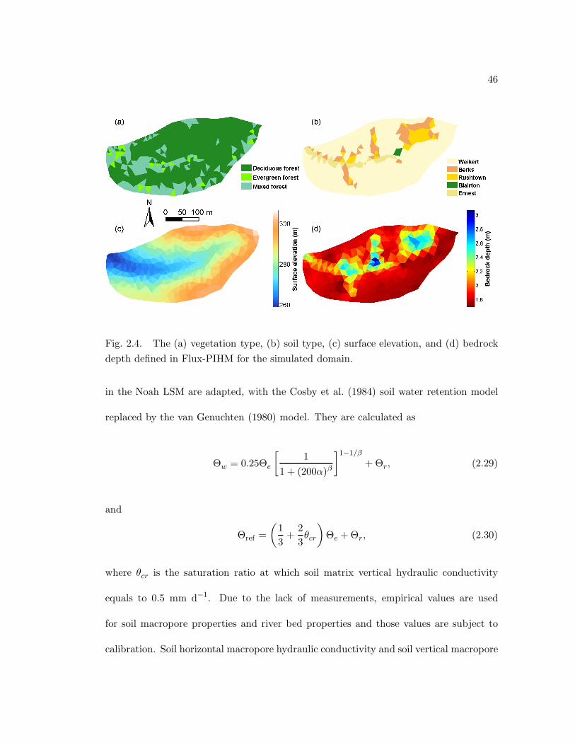
46
Fig. 2.4. The (a) vegetation type, (b) soil type, (c) surface elevation, and (d) bedrock
depth defined in Flux-PIHM for the simulated domain.
in the Noah LSM are adapted, with the Cosby et al. (1984) soil water retention model
replaced by the van Genuchten (1980) model. They are calculated as
Θw = 0.25Θe
[
1
1 + (200α)β
]1−1/β
+ Θr, (2.29)
and
Θref =
(
1
3+
2
3θcr
)
Θe + Θr, (2.30)
where θcr is the saturation ratio at which soil matrix vertical hydraulic conductivity
equals to 0.5 mm d−1. Due to the lack of measurements, empirical values are used
for soil macropore properties and river bed properties and those values are subject to
calibration. Soil horizontal macropore hydraulic conductivity and soil vertical macropore

47
hydraulic conductivity are assumed to be 100 times of their corresponding soil matrix
conductivities as by Li (2010).
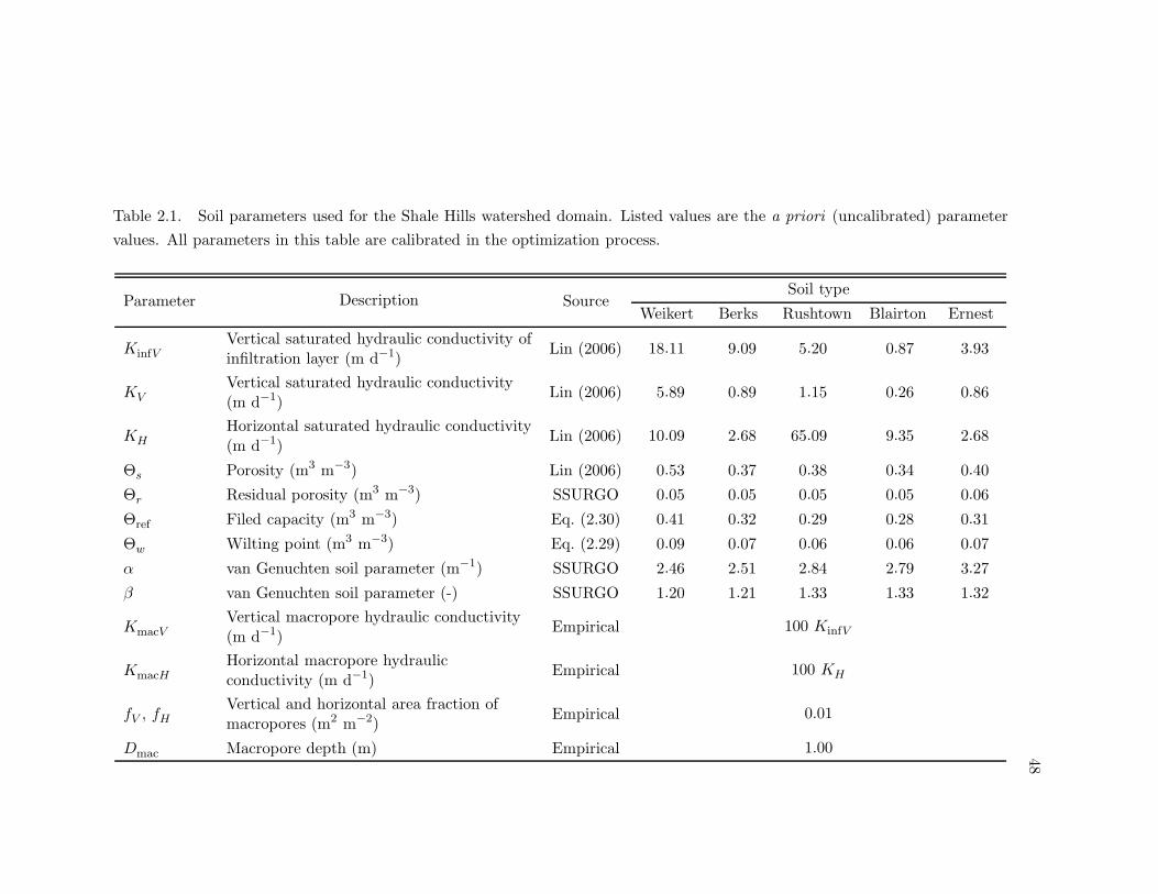
48
Table 2.1. Soil parameters used for the Shale Hills watershed domain. Listed values are the a priori (uncalibrated) parameter
values. All parameters in this table are calibrated in the optimization process.
Parameter Description SourceSoil type
Weikert Berks Rushtown Blairton Ernest
KinfVVertical saturated hydraulic conductivity ofinfiltration layer (m d−1)
Lin (2006) 18.11 9.09 5.20 0.87 3.93
KVVertical saturated hydraulic conductivity(m d−1)
Lin (2006) 5.89 0.89 1.15 0.26 0.86
KHHorizontal saturated hydraulic conductivity(m d−1)
Lin (2006) 10.09 2.68 65.09 9.35 2.68
Θs Porosity (m3 m−3) Lin (2006) 0.53 0.37 0.38 0.34 0.40
Θr Residual porosity (m3 m−3) SSURGO 0.05 0.05 0.05 0.05 0.06
Θref Filed capacity (m3 m−3) Eq. (2.30) 0.41 0.32 0.29 0.28 0.31
Θw Wilting point (m3 m−3) Eq. (2.29) 0.09 0.07 0.06 0.06 0.07
α van Genuchten soil parameter (m−1) SSURGO 2.46 2.51 2.84 2.79 3.27
β van Genuchten soil parameter (-) SSURGO 1.20 1.21 1.33 1.33 1.32
KmacVVertical macropore hydraulic conductivity(m d−1)
Empirical 100 KinfV
KmacHHorizontal macropore hydraulicconductivity (m d−1)
Empirical 100 KH
fV , fHVertical and horizontal area fraction ofmacropores (m2 m−2)
Empirical 0.01
Dmac Macropore depth (m) Empirical 1.00

49
Also due to the lack of measurements, the soil properties of river segments are set
to empirical values which are subject to calibration.
Table 2.2. Parameters used for the river segments. Listed values are the uncalibrated
parameter values. All parameters in this table are calibrated in the optimization process.
Parameter Description Source Value
nriv Mannings Roughness coefficient (s m−1/3) Empirical 0.04
KrivH River side hydraulic conductivity (m d−1) Empirical 0.1
KrivV River bed hydraulic conductivity (m d−1) Empirical 1.0
In 2008, a full survey of all trees over 18 cm diameter at breast height was con-
ducted in SSHO. Twenty-two species were identified and classified as evergreen and de-
ciduous trees. The location of each tagged tree was measured with the global positioning
system (GPS). Tree locations are projected onto the Flux-PIHM domain and the number
of deciduous and evergreen trees in each grid is counted. According to which, land cover
type for each grid is classified into deciduous forest, evergreen forest, or mixed forest, and
the vegetation fractions are calculated. Vegetation parameters for different land cover
types are obtained from the modified International Geosphere-Biosphere Programme
(IGBP) Moderate Resolution Imaging Spectroradiometer (MODIS) 20-category vegeta-
tion (land-use) data (http://www.ral.ucar.edu/research/land/technology/lsm/parameters/),
which are also used in the Noah LSM. Root zone depths are set to 0.6 m for all vegetation
types.

50
Table 2.3. Vegetation parameters used for the Shale Hills watershed domain. Listed values are the uncalibrated parameter
values. The parameter Rc min is calibrated in optimization process.
Parameter Description SourceVegetation type
Deciduousforest
Evergreenforest
Mixedforest
Rc min Minimum stomatal resistance (s m−1) Modified IGBP MODIS 100 150 125
RglReference visible solar radiation(W m−2)
Modified IGBP MODIS 30 30 30
Amin Minimum albedo (-) Modified IGBP MODIS 0.16 0.12 0.17
Amax Maximum albedo (-) Modified IGBP MODIS 0.17 0.12 0.25
emin Minimum emissivity (-) Modified IGBP MODIS 0.93 0.95 0.97
emax Maximum emissivity (-) Modified IGBP MODIS 0.93 0.95 0.97
z0min Minimum roughness length (m) Modified IGBP MODIS 0.5 0.5 0.2
z0max Maximum roughness length (m) Modified IGBP MODIS 0.5 0.5 0.5
hs Water vapor exchange coefficient (-) Modified IGBP MODIS 54.53 47.35 51.93
droot Root zone depth (m) Empirical 0.6 0.6 0.6
Czil
Zilitinkevich parameter (Zilitinkevich1995)
Empirical 0.1 0.1 0.1

51
2.3.3 Forcing data and evaluation data
Meteorological data from in situ measurements and remote sensing data set are
used to drive and evaluate the model (Table 2.4). Spatially uniform forcing is used for
this study. To enable the model to respond to realistic temporal variations in meteo-
rology, as many in situ measurements as possible are used to drive the model. Hourly
precipitation, air temperature and relative humidity data are obtained from the RTH-
net weather station (http://cataract.cee.psu.edu/czo/rth/). Precipitation is measured
with a Hatch OTT precipitation gauge, while air temperature and relative humidity are
measured with a Campbell Scientific HMP45C temperature and relative humidity probe.
Those 10-min interval data are aggregated into hourly data. Downward longwave radia-
tion, downward solar radiation, and surface pressure are not available at SSHO and are
obtained from the Surface Radiation Budget Network (SURFRAD) Penn State Univer-
sity station. SURFRAD Penn State University station locates at 40.72◦ N, 77.93◦ W,
which is 6.48 km away from the Shale Hills watershed. Its surface elevation is 376 m. It
is assumed that radiation and surface pressure at SURFRAD Penn State station repre-
sent the conditions at the Shale Hills watershed. Wind speed data from January 2009 to
March 2009 are obtained from SURFRAD Penn State station. An above-canopy eddy-
covariance flux tower was installed in SSHO in April 2009. Wind speed data from the
flux tower are used for the period from April to December 2009.
MODIS LAI data are introduced to represent vegetation dynamics. MODIS prod-
uct MOD15A2 provides eight-day composite LAI data at 1-km resolution (Knyazikhin

52
Table 2.4. Forcing data used for simulation.
Data Source
Precipitation, 2-m air temperature, and rel-ative humidity
RTHnet weather station
Downward longwave radiation, downwardsolar radiation, and surface pressure
SURFRAD
Wind speedRTHnet flux tower and SURFRAD(prior to 1 April 2009)
LAI Modified MODIS data
et al. 1999; Myneni et al. 2002). The MODIS pixel that centers at the Shale Hills wa-
tershed is chosen for this study. MODIS product recognizes this pixel as covered by
deciduous forest. LAI field measurements have also been collected regularly since April
2010 at SSHO. From 25 April to 31 October 2010, a Decagon AccuPAR meter and a
LI-COR 2200 leaf area meter had been used to measure LAI at 106 sampling points.
Samples were collected every two weeks on average. Fig. 2.5 presents the comparison of
LAI between the MODIS product and the CZO field measurements.
As shown in Fig. 2.5, the MODIS product captures the seasonal variation of LAI
at SSHO, but consistently overestimates LAI in growing season. The MODIS LAI data
in 2009 are then modified based on the comparison:
LAI = (LAIMODIS − LAI0)max(LAICZO) − LAI0
max(LAIMODIS2010) − LAI0+ LAI0, (2.31)
where LAI is the modified MODIS LAI, LAIMODIS is the MODIS LAI measurements,
LAICZO is the SSHO field-measured LAI in 2010, and LAI0 is a reference value set to
be 0.5 m2 m−2. The modified MODIS LAI curve is also presented in Fig. 2.5. Because
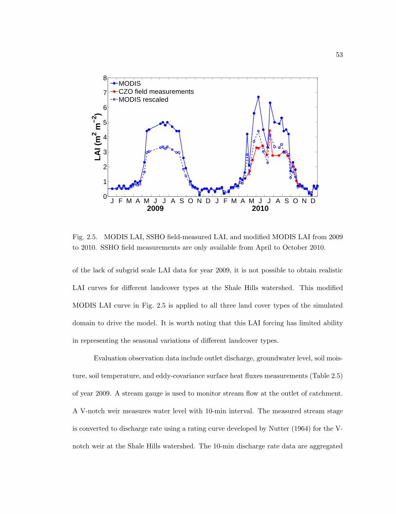
53
0
1
2
3
4
5
6
7
8
LAI (
m2 m
−2)
J F M A M J J A S O N D J F M A M J J A S O N D2009 2010
MODISCZO field measurementsMODIS rescaled
Fig. 2.5. MODIS LAI, SSHO field-measured LAI, and modified MODIS LAI from 2009
to 2010. SSHO field measurements are only available from April to October 2010.
of the lack of subgrid scale LAI data for year 2009, it is not possible to obtain realistic
LAI curves for different landcover types at the Shale Hills watershed. This modified
MODIS LAI curve in Fig. 2.5 is applied to all three land cover types of the simulated
domain to drive the model. It is worth noting that this LAI forcing has limited ability
in representing the seasonal variations of different landcover types.
Evaluation observation data include outlet discharge, groundwater level, soil mois-
ture, soil temperature, and eddy-covariance surface heat fluxes measurements (Table 2.5)
of year 2009. A stream gauge is used to monitor stream flow at the outlet of catchment.
A V-notch weir measures water level with 10-min interval. The measured stream stage
is converted to discharge rate using a rating curve developed by Nutter (1964) for the V-
notch weir at the Shale Hills watershed. The 10-min discharge rate data are aggregated

54
to hourly data to be compared with model predictions of outlet discharge for model
calibration and evaluation.
Groundwater level and soil moisture data are collected from three RTHnet wells
drilled near the stream. Each well is equipped with one water level sensor (Druck pres-
sure transducer CS420-L manufactured by Campbell Scientific) and three soil moisture
sensors (Decagon Echo2 probes). The three soil moisture sensors at each well are located
at three different levels below ground, with depths of 0.1 m, 0.3 m, and 0.5 m below
surface, respectively. The groundwater level and soil moisture data are collected every
10 minutes. Among the three RTHnet wells, Well 1 (Fig. 2.3) is not deep enough to
capture the change of water table in summer months when water table is deeper than
the well depth. For those time periods, only RTHnet Wells 2 and 3 measurements are
adopted. Due to data logger or sensor problems, two of the nine soil moisture sensors
continuously show measurements larger than field measured porosity. Measurements of
soil water content from those two sensors reach up to 2.19 m3 m−3 and 2.42 m3 m−3,
respectively in 2009. Therefore, data from those two sensors are not used in this study.
The water table depth (WTD; distance from the land surface to the groundwater table)
measurements collected in different wells are averaged to represent the observed WTD
at RTHnet wells. The standard deviations between different wells are calculated as the
uncertainty range for the observed WTD. The multiple volumetric soil moisture content
observations from those three wells are averaged to represent the observed soil water
content (SWC). The standard deviations from different soil moisture sensor measure-
ments are calculated as the uncertainty range for the observed SWC. In Flux-PIHM, the
model domain is discretized as such that the three RTHnet wells are located at three

55
vertices of one model grid for the convenience of model-data comparison. This model
grid surrounded by RTHnet wells is selected for the comparison of WTD and SWC. The
WTD predictions in Flux-PIHM and PIHM V2 are calculated from groundwater level
predictions:
WTDm = DBR − hsat, (2.32)
where DBR is the bedrock depth as in model input data, and hsat is the predicted
groundwater level. For Flux-PIHM and PIHM V2, predictions of SWC are calculated as
SWCm =hus
WTDmΘe + Θr, (2.33)
where hus is the predicted unsaturated zone soil water storage. The observed WTD and
SWC data are aggregated into hourly data to be compared with the hourly predictions
of WTD [Eq. (2.32)] and SWC [Eq. (2.33)].
Soil temperature measurements are collected at seven sites at different vertical
levels below ground in 2009. Soil temperatures are measured with 229 probes manu-
factured by Campbell Scientific, and 5TE probes manufactured by Decagon. Among
those seven soil temperature sites, data from Site 15 are only 0.1 ◦C accurate, while the
others are 0.001 ◦C accurate; Site 61 does not have measurements at 5 cm level. Data
from those two sites are not used. The locations of the remaining five sites are shown in
Fig. 2.3. For those five sites, the soil temperature data measured at 5 cm below surface
are averaged and aggregated into hourly data. Model predictions of soil temperature at
the top soil layer (0–10 cm) from the five corresponding model grids are averaged to be
compared with the observations.

56
The above-canopy eddy-covariance flux tower measures wind speed and air tem-
perature with a Campbell Scientific CSAT3 three dimensional sonic anemometer. Carbon
dioxide and water vapor concentrations are measured with a LI-COR LI-7500 CO2/H2O
Analyzer. The wind coordinate is adjusted following the planar fit coordinate method
(Lee et al. 2004), and the quality control method from Vickers and Mahrt (1997) is
adopted to screen out the eddy-covariance data with low quality. The gaps in processed
30-min sensible and latent heat fluxes are filled using look-up table method suggested
by Falge et al. (2001). The gap-filled sensible and latent heat fluxes are aggregated into
hourly data to be compared with hourly predictions of sensible and latent heat fluxes
averaged over the model domain.
Table 2.5. Evaluation data used for model optimization and evaluation.
Data Source
River discharge RTHnet outlet gauge
Water table depth and soil water content RTHnet wells
Soil temperature RTHnet soil temperature sites
Surface heat fluxes RTHnet flux tower
2.4 Optimization and evaluation of Flux-PIHM
2.4.1 Model optimization and spin-up
Flux-PIHM has a large number of tunable model parameters. Some of those
parameters are dependent on soil type (e.g., KV , α, and β) or landcover type (e.g., Rc min,
Θref , and Θw). Thus calibration could be very complicated if the model domain contains

57
a large number of soil types or landcover types. To simplify the calibration problem,
one single global calibration coefficient is used for each model parameter regardless of
soil type or landcover type. The global calibration coefficient is a multiplier acting on
the corresponding soil or vegetation related parameter for all soil or vegetation types.
For example, the ith uncalibrated soil/vegetation parameter φi have different values
φij , (j = 1, 2, · · · J) for soil/vegetation types 1 to J . The corresponding calibrated
soil/vegetation parameter Φij is given by
Φij = ciφij, (2.34)
where φij is the ith uncalibrated soil/vegetation parameter for the jth soil/vegetation
type, and ci is the global calibration coefficient for the ith soil/vegetation parameter.
By applying global multiplier calibration coefficients, the dimension of parameter space
for calibration is reduced and the ratios between uncalibrated a priori parameters of
different soil/vegetation types are preserved. The default value for calibration coefficient
is 1.0.
A comprehensive calibration is conducted to enhance the performance of Flux-
PIHM at the Shale Hills watershed. Due to the high computational cost of physically-
based hydrologic models, it is difficult to apply advanced optimization methods to those
models. Currently trial and error procedure is still the prevalent choice and is adopted for
the calibration of Flux-PIHM in this chapter. In the comprehensive calibration process,
outlet discharge, water table depth, soil water content, soil temperature at 5 cm below
surface, and eddy-covariance surface heat flux data from June to July 2009 are used to

58
adjust model parameters. This period is chosen because it covers both peak discharge
event and base flow period, and also has considerable evapotranspiration rate.
Fig. 2.6 illustrates the workflow for manual calibration of Flux-PIHM. First, Flux-
PIHM run is performed for the calibration period with initial guesses of model parameter
values. The model forecasts are then compared with observations. The agreement and
difference between model forecasts and observations are inspected visually. Considering
the effect of each parameter and the interaction between different model parameters,
parameter values are adjusted in the effort to minimize model errors based on human
judgment. A new Flux-PIHM run with the new guesses of parameters is performed.
This process is repeated as needed, until the agreement between model outputs and
observations are satisfactory.
Initial guessesφ
0
Forecast
xf
New guesses
φnew
Flux-PIHMVisual inspection
Manual tuning
Observations
y
Fig. 2.6. Workflow for manual calibration of Flux-PIHM.

59
The calibration of model parameters are accomplished in two steps. The first
step emphasizes the match of discharge recession curve and mean WTD. In this step,
Flux-PIHM is started in the “relaxation mode”, in which the model relaxes from a sat-
uration state. The recession curve of model discharge is compared with the measured
discharge recession curve for the June peak discharge event. The model WTD after
discharge recession is compared with the measured WTD at RTHnet wells. The calibra-
tion coefficients of KH , KmacH , fV , and Dmac, which are related to horizontal water
transport and mean water table depth, are determined. In the second step, the other
hydrologic and land surface parameters are adjusted by comparing model peak discharge
rate, low flow rate, fluctuation of SWC and WTD, and variations in surface heat fluxes
with measurements. Because the model is manually tuned and the calibration process
involves a lot of model runs, spin-up for every calibration model run is not cost-efficient.
To accelerate the calibration process, model runs using different guesses of parameters
start from the same initial conditions.
A calibration file containing calibration coefficients of those model parameters is
used as model input. The model parameters which are calibrated and their corresponding
calibration coefficients are listed in Table 2.6.
After calibration, Flux-PIHM spins-up using the atmospheric forcing from 0000 UTC
20 October 2008 to 0000 UTC 1 January 2009. Kampf (2006) found that starting from
saturation decreases the time need for spin-up process. Thus the model is initialized
with the relaxation mode for spin-up. Initial surface skin temperature is set to the air
temperature and soil temperatures are obtained from a linear interpolation between sur-
face skin temperature and bottom boundary condition. Flux-PIHM usually relaxes from
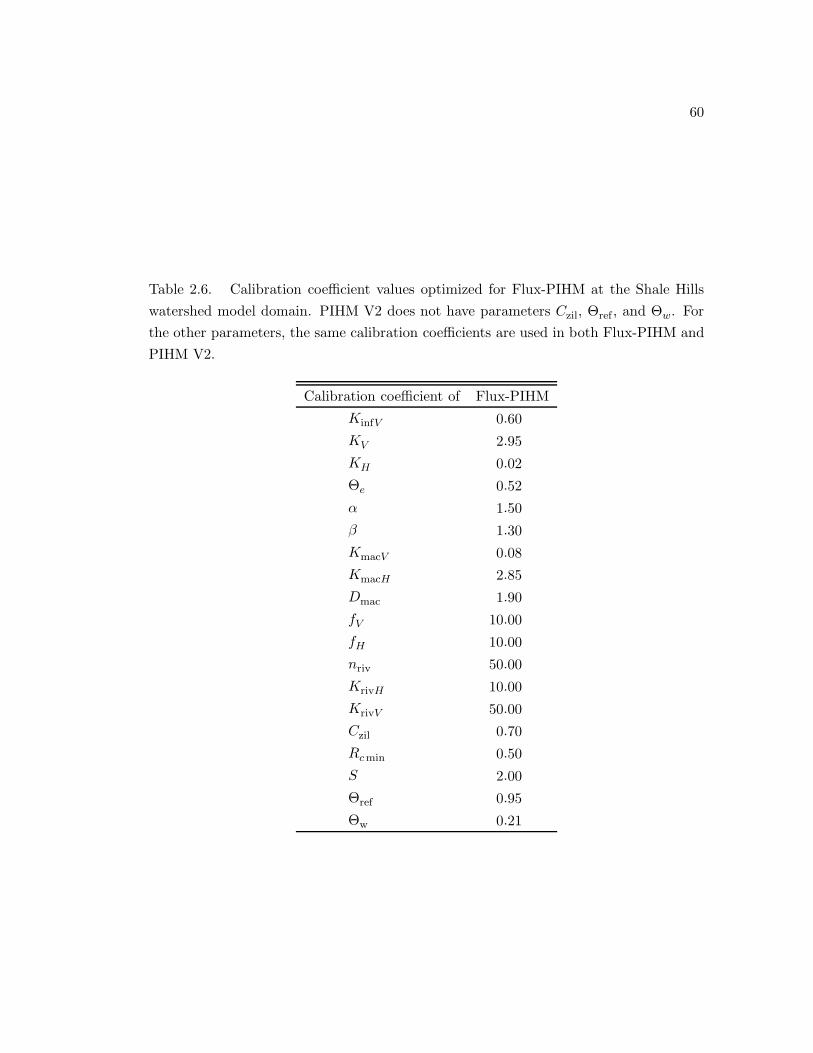
60
Table 2.6. Calibration coefficient values optimized for Flux-PIHM at the Shale Hills
watershed model domain. PIHM V2 does not have parameters Czil, Θref , and Θw. For
the other parameters, the same calibration coefficients are used in both Flux-PIHM and
PIHM V2.
Calibration coefficient of Flux-PIHM
KinfV 0.60
KV 2.95
KH 0.02
Θe 0.52
α 1.50
β 1.30
KmacV 0.08
KmacH 2.85
Dmac 1.90
fV 10.00
fH 10.00
nriv 50.00
KrivH 10.00
KrivV 50.00
Czil 0.70
Rc min 0.50
S 2.00
Θref 0.95
Θw 0.21

61
hydrologic saturation state within about 7 days. A two-month spin-up period is used to
ensure the model eliminating the effects of initial conditions. The same model parameter
sets and initial conditions are used for both Flux-PIHM, and PIHM V2, if applicable, to
ensure unbiased comparison.
2.4.2 Water budget
Predicted water budgets from Flux-PIHM and PIHM V2 are compared for the
period from 1 March to 1 December 2009. Snow covered conditions are excluded from
the model evaluation because Flux-PIHM is using a simple snow physics which is not
sufficient for accurate hydrologic prediction in winter. Therefore, this study focuses
on warm seasons. Fig. 2.7 presents the predicted water budget from Flux-PIHM and
PIHM V2 and the observed discharge from RTHnet. Runoff in Fig. 2.7 is calculated as
the total discharge divided by the total area of the watershed. Predicted total runoff
from both models are close to the observation, and Flux-PIHM provides a better total
runoff prediction compared with PIHM V2. Flux-PIHM overestimates the total runoff
by only 0.4% (1 mm) while PIHM V2 overestimates the total runoff by 4.1% (11 mm).
The total evapotranspiration predicted by both models are also close. The to-
tal evapotranspiration prediction from Flux-PIHM is 566 mm, and the prediction from
PIHM V2 is 558 mm. The partitionings of total evapotranspiration, however, are very
different in those two models. Flux-PIHM predicts higher canopy evaporation and tran-
spiration compared with PIHM V2, while PIHM V2 predicts higher soil evaporation.
Compared with Flux-PIHM, PIHM V2 predicts much higher soil evaporation but lower

62
RTHnet Flux−PIHM PIHM V20
200
400
600
800
1000
271 272 282
67 55
372 311
127 192
Wat
er B
udge
t (m
m)
RunoffCanopy evaporationTranspirationSoil evaporation
Fig. 2.7. Comparison of water budget between Flux-PIHM and PIHM V2 from
0000 UTC 1 March to 0000 UTC 1 December 2009. Observed discharge from RTH-
net is also presented.
canopy transpiration and canopy evaporation. Soil evaporation and transpiration ex-
tract water from different subsurface layers. Soil evaporation only has access to the top
soil layer, while transpiration could transport deep soil water or even groundwater to the
atmosphere, depending on the root zone depth and the water table depth. For the six
model grids near the river outlet, the fraction of evapotranspiration that is extracted di-
rectly from groundwater is calculated. In Flux-PIHM 34.8% of total evapotranspiration
is extracted directly from groundwater, while in PIHM V2, this fraction is only 22.1%
because of the lower transpiration prediction in PIHM V2. Those differences could pro-
duce different soil moisture profiles in different models, and affect evapotranspiration
and flood/drought forecasting.

63
2.4.3 Evaluation of hydrologic predictions: Discharge, water table depth,
and soil water content
To test the model’s ability to predict the hydrological states of the watershed,
model discharge, WTD and SWC predictions are compared with in situ measurements.
Several criteria are used to quantify model predictions of discharge, including the total
bias, the Nash-Sutcliffe model efficiency coefficient (NSE; Nash and Sutcliffe 1970), and
the correlation coefficient with observation. Total bias is defined as:
Total bias =
∑Tt=1
(
Qtm − Qt
o
)
∑Tt=1
Qto
× 100%, (2.35)
where Qo is the observed discharge, Qm is the predicted discharge, T is the length of
observation, and a superscript t indicates observation or modeled discharge at the time
step t. NSE is the most commonly used coefficient to evaluate hydrologic models.It is
defined as
NSE = 1 −∑T
t=1
(
Qtm− Qt
o
)2
∑Tt=1
(
Qto− Qo
)2. (2.36)
The correlation coefficient is defined as
R =
∑Tt=1
(
Qtm − Qm
) (
Qto − Qo
)
√
∑Tt=1
(
Qtm− Qm
)2√
∑Tt=1
(
Qto− Qo
)2. (2.37)
Besides, to evaluate the performance of discharge prediction of Flux-PIHM com-
pared with other hydrologic models, one of the most widely used conceptual model, the
Soil Water Assessment Tool (SWAT; Arnold et al. 1998; Arnold and Fohrer 2005), is used
as a benchmark model. SWAT has not been implemented at the Shale Hills watershed,

64
but Green and Van Griensven (2008) calibrated SWAT version 2005 (SWAT2005) in six
small watersheds with areas between 0.04 km2 and 0.08 km2 in central Texas. SWAT2005
was calibrated at those six watersheds for two different calibration periods. One cali-
bration period is one-year long, and the other one is four-year long. No independent
validation is provided in their work. The statistics for SWAT2005 discharge predictions
in those six watersheds in different calibration period are presented in Table 2.7.
Table 2.7. Total bias, NSE, and correlation coefficient of SWAT2005 daily discharge
predictions at six small watersheds in central Texas compared with observations.
Calibration period Total bias (%) NSE R
Four years −16.32–5.34 0.80–0.86 0.90–0.93
One year −29.15–20.00 0.53–0.80 0.73–0.89
Fig. 2.8 presents the comparison of hourly outlet discharge among RTHnet mea-
surements and two models from March to December 2009. The statistics of discharge
predictions are presented in Table 2.8. The statistics of Flux-PIHM daily discharge pre-
dictions at the Shale Hills watershed are better than the SWAT2005 one-year calibration
at the six watersheds in central Texas, and are comparable to the SWAT2005 four-
year calibration statistics. The statistics of Flux-PIHM hourly discharge predictions at
the Shale Hills watershed are still comparable to SWAT2005 daily discharge predictions
with one-year calibration. It is worth noting that the calibration period for Flux-PIHM
is much shorter than in the work of Green and Van Griensven (2008). The Shale Hills
watershed also has much steeper slopes (25–48%) compared with those six watershed in
central Texas (1.1–3.2%), which suggests that the discharge at the Shale Hills watershed

65
may exhibit more temporal variability. Flux-PIHM prediction agrees well with measure-
ments for both dry period flows and peak flows as illustrated in Fig. 2.8. Though June
and July data are used for calibration, Flux-PIHM still overestimates the peak event
in June, because different initial conditions are used in calibration and evaluation. In
March, April and May, Flux-PIHM underestimates base flows but overestimates some
discharge peaks (Fig. 2.8). The largest errors occur in October, when Flux-PIHM un-
derestimates the highest peak as well as overestimates a series of peak events before
that.
Month
Dis
char
ge (
m3 d
−1)
M A M J J A S O N 0
500
1000
1500
2000
250011000
13000
RTHnetFlux−PIHMPIHM V2
10/15 10/190
400
800
1200
1600
Fig. 2.8. Comparison of hourly outlet discharge among RTHnet measurements, Flux-
PIHM, and, PIHM V2 predictions from 0000 UTC 1 March to 0000 UTC 1 December
2009. The inset highlights the peak discharge event from October 15 to October 19, for
which Flux-PIHM and PIHM V2 have considerably different predictions.
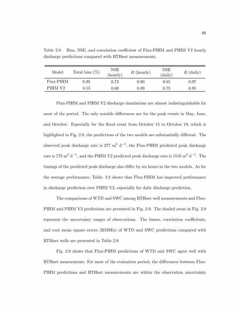
66
Table 2.8. Bias, NSE, and correlation coefficient of Flux-PIHM and PIHM V2 hourly
discharge predictions compared with RTHnet measurements.
Model Total bias (%)NSE
(hourly)R (hourly)
NSE(daily)
R (daily)
Flux-PIHM 0.30 0.73 0.90 0.85 0.97
PIHM V2 4.13 0.69 0.89 0.75 0.95
Flux-PIHM and PIHM V2 discharge simulations are almost indistinguishable for
most of the period. The only notable differences are for the peak events in May, June,
and October. Especially for the flood event from October 15 to October 19, which is
highlighted in Fig. 2.8, the predictions of the two models are substantially different. The
observed peak discharge rate is 277 m3 d−1, the Flux-PIHM predicted peak discharge
rate is 778 m3 d−1, and the PIHM V2 predicted peak discharge rate is 1516 m3 d−1. The
timings of the predicted peak discharge also differ by six hours in the two models. As for
the average performance, Table. 2.8 shows that Flux-PIHM has improved performance
in discharge prediction over PIHM V2, especially for daily discharge prediction.
The comparisons of WTD and SWC among RTHnet well measurements and Flux-
PIHM and PIHM V2 predictions are presented in Fig. 2.9. The shaded areas in Fig. 2.9
represent the uncertainty ranges of observations. The biases, correlation coefficients,
and root mean square errors (RMSEs) of WTD and SWC predictions compared with
RTHnet wells are presented in Table 2.9.
Fig. 2.9 shows that Flux-PIHM predictions of WTD and SWC agree well with
RTHnet measurments. For most of the evaluation period, the differences between Flux-
PIHM predictions and RTHnet measurements are within the observation uncertainty

67
WT
D (
m)
(a)
0.0
1.0
2.0
RTHnetFlux−PIHMPIHM V2
M A M J J A S O NMonth
SW
C (
m3 m
−3)
(b)
0.1
0.2
0.3
0.4RTHnetFlux−PIHMPIHM V2
Fig. 2.9. As in Fig. 2.8, but for (a) water table depth (WTD) and (b) soil water content
(SWC). The shaded areas indicate the uncertainty range of observations.
ranges, for both WTD and SWC. Like discharge predictions, the largest errors appear in
October, when model errors in WTD and SWC fall out of the observation uncertainty
ranges. In October, Flux-PIHM continuously underestimates WTD and overestimates
SWC, when the error in WTD reaches about −0.5 m, and the error in SWC reaches up
to 0.1 m3 m−3. In spring (March to May), although model errors of WTD and SWC are
always within the observation uncertainty ranges, model predictions have consistent wet
bias (low bias in WTD and high bias in SWC) compared with observed average WTD
and SWC. Fig. 2.9 also shows that the PIHM V2 predictions in WTD and SWC follow
the observations better than Flux-PIHM in March, but PIHM V2 is outperformed by
Flux-PIHM in almost all following months. The largest differences between Flux-PIHM
and PIHM V2 appear in October, when the differences between the two models reach up

68
to 25–30 cm. As indicated in Table 2.9, Flux-PIHM provides better overall predictions
of WTD and SMC than PIHM V2, although PIHM V2 WTD bias is slightly smaller.
Table 2.9. Bias, RMSE and correlation coefficient of Flux-PIHM and PIHM V2 hourly
WTD and SMC predictions compared with RTHnet well measurements.
WTD SMC
Bias (m) RRMSE(m)
Bias(m3 m−3)
RRMSE
(m3 m−3)
Flux-PIHM
−0.12 0.84 0.21 0.01 0.76 0.02
PIHMV2
−0.11 0.80 0.23 0.01 0.73 0.03
2.4.4 Evaluation of surface energy balance predictions: Sensible and latent
heat fluxes and soil temperature
The aggregated hourly sensible (H) and latent (LE) heat fluxes measured at
SSHO are compared with model hourly predictions averaged over the model domain.
H and LE measurements at SSHO are available from 1 April 2009. The period from
1 April 2009 to 1 January 2010 is divided into four sub-periods to evaluate surface heat
fluxes predictions for different seasons: 1 April to 1 June 2009 as spring, 1 June to
1 September 2009 as summer, 1 September to 1 December 2009 as fall, and 1 December
2009 to 1 January 2010 as winter. Fig. 2.10 presents the comparisons of surface heat
fluxes among Flux-PIHM, PIHM V2 and RTHnet eddy covariance measurements as
averaged daily cycles for each season. Plots of hourly H and LE are not presented to
save space, instead Table 2.10 lists the statistics for each season based on the comparison
69
between hourly predictions and observations of H and LE. Flux-PIHM predicts both
H and LE, but PIHM V2 only predicts evapotranspiration rate, which is equivalent to
LE.
Fig. 2.10 shows that Flux-PIHM predictions of mid-day H and LE have consistent
high biases during all seasons. It needs to be noted that Flux-PIHM closes the energy
budget at the land surface, while field measurements always fail to close the energy
budget, and the measured H + LE tend to be less than Rn − G (McNeil and Shut-
tleworth 1975; Fritschen et al. 1992; Twine et al. 2000). Therefore, in the calibration
process, Flux-PIHM are subjectively calibrated to overestimate H and LE, assuming
the eddy covariance method underestimates surface heat fluxes. There are also phase
errors between observed and predicted LE in Fig. 2.10. Except for spring and winter
LE, Flux-PIHM hourly predictions of H and LE have high correlations with RTHnet
measurements, with correlation coefficients between 0.91 and 0.94 (Table 2.10), which
shows that Flux-PIHM is capable of capturing the variation of surface heat fluxes well at
hourly resolution. Flux-PIHM errors of mid-day LE in spring are much higher than in
other seasons (Fig. 2.10). The RMSE for spring LE is larger than the RMSEs in other
seasons, and the correlation coefficient for LE in spring is also relatively lower than in
summer and fall (Table. 2.10). This substantial high bias in spring agrees with the signs
of biases in WTD and SWC predictions in the corresponding months (Fig. 2.9). The
correlation coefficient of winter LE is as low as 0.55, but LE measurements of open-path
gas analyzer in winter is less reliable than in other seasons (Burba et al. 2008). The
insufficient winter physics in Flux-PIHM may also contribute to the low correlation of
LE in winter.

70
0
100
200
300Spring
H (Flux−PIHM)H (RTHnet)LE (Flux−PIHM)LE (PIHM V2)LE (RTHnet)
Summer
3 6 9 12 15 18 21
0
100
200
300Fall
3 6 9 12 15 18 21
Winter
Time (UTC)
Hea
t Flu
x (W
m−2
)
Fig. 2.10. Comparison of surface heat fluxes among Flux-PIHM, PIHM V2 and RTHnet
measurements as averaged daily cycles at each hour of the day for different seasons.
Table 2.10. RMSE and correlation coefficient of Flux-PIHM and PIHM V2 hourly H
and LE predictions compared with eddy covariance flux tower measurements for different
seasons.
Spring Summer Fall Winter
H LE H LE H LE H LE
Flux-
PIHM
RMSE(W m−2)
41.37 61.02 39.42 45.43 33.13 22.75 29.60 14.20
R 0.94 0.78 0.92 0.94 0.92 0.92 0.91 0.55
PIHM
V2
RMSE(W m−2)
N/A 64.16 N/A 50.01 N/A 23.72 N/A 12.06
R N/A 0.72 N/A 0.92 N/A 0.89 N/A 0.52

71
When averaged into daily cycles, Flux-PIHM and PIHM V2 LE are almost indis-
tinguishable in summer and winter (Fig. 2.10). But predictions of LE in Flux-PIHM are
higher in spring and fall. In spring, summer, and fall, Flux-PIHM LE predictions have
higher correlation coefficients and lower RMSEs compared to PIHM V2, which indicates
that Flux-PIHM is more capable of reproducing the hourly variation in evapotranspi-
ration. It is as expected because Flux-PIHM has a more complex land surface scheme
than PIHM V2.
Fig. 2.11 presents the comparison of hourly soil temperature at 5 cm below surface
between Flux-PIHM predictions and RTHnet observations. From March to November,
the average bias for soil temperature prediction at 5 cm below the surface is 0.81 ◦C and
the RMSE is 1.6 ◦C. The correlation coefficient between model and measurement is 0.97.
Fig. 2.11 suggests that the soil temperature predicted by Flux-PIHM has a consistent
high bias in summer, but the errors are random in other seasons. At the beginning of
March, the error could be as large as ±5 ◦C. This is probably due to the simple snow
physics in Flux-PIHM which could not simulate the thawing process well.
2.5 Correlation between surface heat fluxes and water table depth
The coupled land surface hydrologic model is a good tool for the study of the
interaction between the subsurface and the land surface. Annual average sensible and
latent heat fluxes as functions of WTD in each model grid from Flux-PIHM simulation
for year 2009 is presented in Fig. 2.12. Fig. 2.12 shows that the differences of annual
average H and LE among different grids can be over 30 W m2, which indicates that the
spatial variability of predicted H and LE is large at the Shale Hills watershed. There is
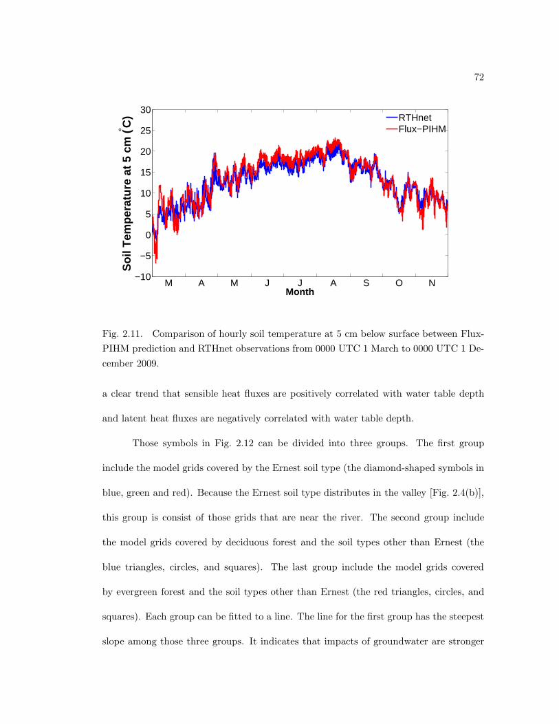
72
−10
−5
0
5
10
15
20
25
30
M A M J J A S O N
Soi
l Tem
pera
ture
at 5
cm
(° C
)
Month
RTHnetFlux−PIHM
Fig. 2.11. Comparison of hourly soil temperature at 5 cm below surface between Flux-
PIHM prediction and RTHnet observations from 0000 UTC 1 March to 0000 UTC 1 De-
cember 2009.
a clear trend that sensible heat fluxes are positively correlated with water table depth
and latent heat fluxes are negatively correlated with water table depth.
Those symbols in Fig. 2.12 can be divided into three groups. The first group
include the model grids covered by the Ernest soil type (the diamond-shaped symbols in
blue, green and red). Because the Ernest soil type distributes in the valley [Fig. 2.4(b)],
this group is consist of those grids that are near the river. The second group include
the model grids covered by deciduous forest and the soil types other than Ernest (the
blue triangles, circles, and squares). The last group include the model grids covered
by evergreen forest and the soil types other than Ernest (the red triangles, circles, and
squares). Each group can be fitted to a line. The line for the first group has the steepest
slope among those three groups. It indicates that impacts of groundwater are stronger

73
WTD (m)
H (
W m
−2)
0 1 2 320
30
40
50
60
WTD (m)
LE
(W
m−2
)
0 1 2 320
30
40
50
60
WeikertBerksRushtownErnest
Deciduous forestEvergreen forestMixed forest
Fig. 2.12. Annual average sensible and latent heat fluxes plotted as functions of water
table depth from Flux-PIHM simulation. Each symbol represents one grid in the Shale
Hills watershed model domain. Different soil types are represented by different shapes
and different land cover types are plotted using different color. Blairton soil type is not
plotted because only two grids are categorized as Blairton.

74
on those grids near the river than the other model grids. For the grids near the river,
groundwater table is relatively shallow and vegetation roots have access to groundwater,
thus groundwater has direct impacts on surface energy balance. For the grids far from
the river, groundwater table is deep and vegetation roots have no access to groundwater,
thus the impacts of groundwater are weak. For those grids, the effect of groundwater on
surface heat fluxes is indirect, and is accomplished by affecting the soil moisture profile.
The cluster of the same vegetation type suggests that landcover properties have
stronger impacts on surface heat fluxes than soil properties. The model grids covered
by deciduous forest and evergreen forest have similar annual available energy (H + LE)
at each WTD, but the grids covered by deciduous forest tend to have higher LE thus
lower H compared with the grids covered by evergreen forest. It might be caused by the
smaller minimum stomatal resistance (Rc min) value of the deciduous forest (Table 2.3).
This correlation between surface heat fluxes and groundwater table has been
found in other studies (e.g., Kollet and Maxwell 2008). Kollet and Maxwell (2008) also
found that when water table depth is deeper than 5 m in the Little Washita watershed,
Oklahoma, the land surface and groundwater are decoupled. This decoupling of land
surface and groundwater is not found in this study at the Shale Hills watershed.
2.6 Discussions and conclusions
It is expected that coupled models of land surface and subsurface may yield im-
provements in weather and short-term climate forecasting and flood/drought forecasting.
In this chapter, a coupled land surface hydrologic model, Flux-PIHM is presented, and
implemented at the Shale Hills watershed (0.08 km2) in central Pennsylvania. While
75
previous studies tend to use only discharge data for model calibration and evaluation,
Flux-PIHM is manually calibrated with multiple observations, including discharge, wa-
ter table depth, soil water content, soil temperature, and sensible and latent heat fluxes.
Besides, the model is calibrated and evaluated at hourly timescale to improve the model’s
ability of simulating sub-daily scale processes.
The performance of Flux-PIHM discharge prediction at the Shale Hills watershed
is comparable to a most-widely-used conceptual model at similar watersheds. Notable
errors in Flux-PIHM predictions occur in March, April, May, and October. From March
to May, the model overestimates SWC and underestimates WTD. Because of the high
bias in soil moisture, Flux-PIHM produces substantially high bias in LE. Base flow
rate from March to May is underestimated. In October, the model underestimates the
highest peak event but overestimates some peak discharge events before the highest peak.
The largest errors in WTD and SWC during the evaluation period occur in October as
well, when the error in WTD reaches about −0.5 m, and the error in SWC is as high as
0.1 m3 m−3. Because only one year data are used for the model evaluation, it is not clear
whether the errors are systematic errors caused by insufficient model physics and model
parameter, or random model errors. In this study only June and July data are used
for calibration. Compared with similar studies, the calibration period for Flux-PIHM
is relatively short, and only focuses on summer months. The model parameters might
be biased towards better summer predictions instead of overall annual performance. A
longer calibration period may improve model predictions. Besides, the model errors
in April and May might be related to the insufficient winter physics in Flux-PIHM.
76
Because the thawing process cannot be simulated accurately, the errors would impair
the predictions in spring season.
Model predictions of Flux-PIHM are also compared with PIHM V2, which does
not have surface energy balance simulation. Results indicate that Flux-PIHM slightly
improves the overall hourly predictions of outlet discharge, WTD, and SWC compared
with PIHM V2. Although the improvement of model discharge predictions are not clear
in Fig. 2.8, Flux-PIHM prediction has smaller total bias, higher correlation coefficient
with observation, and higher NSE, compared with PIHM V2 (Table 2.8). Differences
in discharge predictions are only noticeable for some high discharge peaks. For a flood
event from 15 to 19 October, Flux-PIHM and PIHM V2 provides substantially differ-
ent predictions in peak discharge rate and timing. Because the hydrologic schemes in
those two models are completely the same, the differences in the predictions of discharge
rate and timing are caused by the different evapotranspiration calculations. The differ-
ences in the predictions of this flood event demonstrate the impact of evapotranspiration
simulation on flood prediction. Table 2.9 shows that improvement of WTD and SWC
predictions from Flux-PIHM over PIHM V2 is not significant, but the differences in
WTD predictions between two models reach upto 0.25–0.3 m for some time periods.
The partitionings of evapotranspiration into canopy evaporation, canopy transpiration,
and soil evaporation are considerably different in Flux-PIHM and PIHM V2.
Generally, Flux-PIHM is able to provide good discharge, WTD, SWC, sensible
and latent heat fluxes, and soil temperature predictions at hourly resolution at the
small-scale watershed. Nonetheless, the inclusion of the complex surface energy balance
simulation only brings slight improvements in model predictions at this small watershed
77
in this one year period. Whether the coupled land surface hydrologic model improves
predictions at larger scales for longer time periods, and how much does it improve the
predictions if ever, still need exploration.
Due to the lack of spatially distributed measurements, capability of Flux-PIHM
in representing spatial heterogeneity in subsurface and land surface cannot be evaluated
currently. Spatially distributed measurements of groundwater table and other variables
are being collected at SSHO and those measurements could be used for future study.
In Flux-PIHM, surface topography of each grid is not taken into account in the
simulation of surface heat fluxes. Thus, the model has limited ability in simulating the
spatial heterogeneity induced by different incoming solar radiation on hill slopes. This
could cause considerable errors in the spatial distribution of surface heat fluxes at Shale
Hills watershed, which has almost true north-facing and south-facing slopes.
A well-calibrated, fully-coupled land surface hydrologic model as Flux-PIHM is an
ideal tool to study the interaction between the subsurface and the land surface. Model
results show that annual average sensible and latent heat fluxes are correlated with water
table depth at the Shale Hills watershed. The correlation between water table depth and
surface heat fluxes is especially strong for the model grids near the river. The interaction
between water table depth and surface heat fluxes justifies the significance for developing
a coupled land surface hydrologic model.
Flux-PIHM adds the ability of simulating surface energy balance to PIHM and
improves the predictions of discharge, WTD, SWC and evapotranspiration, however
slightly. The more accurate evapotranspiration prediction could improve the forecasting
of some peak discharge events, especially after extended dry period. The accurate total

78
discharge prediction is critical for long term flood/drought forecasting, as well as surface
energy balance forecasting. A well calibrated land surface hydrologic model as such could
improve our understanding of groundwater-land surface-atmosphere interaction. It is
expected that a coupled model of land surface and groundwater like Flux-PIHM could
yield improvements in weather and short-term climate forecasting and flood/drought
forecasting.
In this study, Flux-PIHM is only tested at a small-scale watershed for a one-year
period. How does Flux-PIHM perform for different watersheds with different size, dif-
ferent topography and different climate, and how do the land surface and the subsurface
interact in different watersheds would be interesting questions to answer. Whether the
coupled land surface hydrologic model improves the predictions at larger scales for longer
time periods, and how much does it improve the predictions if ever, still need exploration.

79
Chapter 3
Evaluation of Flux-PIHM Parameter Sensitivities
3.1 Introduction
Numerical models are important tools for the forecasting of complex processes in
natural systems. They can also improve our understanding of those complex processes
and help incorporate this understanding into decision making. Accuracy of numerical
models is limited by the uncertainties in model parameters. Generally, there are two
types of parameters in numerical models: physical parameters and process parameters.
Physical parameters are measurable parameters with physical meanings. Process pa-
rameters are those parameters that cannot be measured directly due to practical or
theoretical reasons. Parameter uncertainties could be large, if a process parameter is
poorly defined, if a physical parameter is not accurately measured, or if a parameter is
not sufficiently representative (Prihodko et al. 2008).
Both land surface models (LSMs) and hydrologic models are highly parameterized
models. Model structures are complex and the number of involved parameters is often
large. Especially for hydrologic models, the uncertainties in model parameters are the
main source of uncertainties (Moradkhani and Sorooshian 2008). For hydrologic models,
the physical parameter values in actual field conditions might be substantially different
from those measured in laboratory; the range of variation in parameter values could span
orders of magnitude (Bras 1990). Some physical parameters have considerable spatial

80
heterogeneity which weakens the representativity of the measured parameter values.
Consequently, parameter uncertainties in those models are often large.
Parameter sensitivity tests analyze the influence of model parameters on model
predictions, and provide insights into model structures and system dynamics. Parame-
ter sensitivity tests are also a vital step towards successful parameter estimation. For a
sophisticated numerical model, the number of parameters involved is often large. Fur-
thermore, the number of model parameter sets that can be estimated is infinite (Nielsen-
Gammon et al. 2010). Due to the limitation of computers, optimization algorithm,
and model parameterizations, not all model parameters could be successfully estimated.
Therefore, research priorities need to be guided by sensitivity tests to select the most
influential parameters for estimation.
Aksoy et al. (2006) introduced the concept of parameter identifiability as an in-
dicator for whether or not a parameter could be estimated successfully using the ensem-
ble Kalman filter (EnKF; Evensen 1994). Zupanski and Zupanski (2006) and Nielsen-
Gammon et al. (2010) generalized the characteristics of parameters for successful esti-
mation as observability, simplicity, and distinguishability. Nielsen-Gammon et al. (2010)
also concluded these characteristics as the three dimensions of parameter identifiability.
Observability describes how strongly the change of parameter values could be reflected
onto observation space. High observability means that a change in parameter values could
lead to relatively large change in model predictions. Simplicity describes how smoothly
model predictions vary with the change of parameter values. An ideal simplicity is that
the model predictions vary linearly with the change of parameter values. Distinguisha-
bility describes how effectively could the impact of one parameter be distinguished from

81
other parameters. Low observability, low simplicity, or low distinguishability could make
parameter estimation difficult to perform. Parameter sensitivity tests examine those
characteristics, and can be used to identify model parameters suitable for parameter
estimation.
In Chapter 2, the coupled land surface hydrologic model Flux-PIHM is manually
calibrated. The manual calibration process described in Fig. 2.6 is highly time-consuming
and labor-intensive. The now widely-used data assimilation method EnKF provides the
possibility for automatic sequential calibration for complex models like Flux-PIHM, a
spatially-distributed, physically-based, and fully-coupled land surface hydrologic model.
In this chapter, parameter sensitivity tests are performed in preparation for Flux-PIHM
parameter estimation using EnKF, under the framework provided by Nielsen-Gammon
et al. (2010). The sensitivity tests aim to select the most identifiable Flux-PIHM model
parameters to be estimated using EnKF, and help interpret future EnKF parameter
estimation results. By examining the sensitivity of hydrologic variables to land surface
parameters, and sensitivity of land surface variables to hydrologic parameters, the sen-
sitivity tests are also expected to enhance our understanding of land surface-subsurface
interactions within Flux-PIHM.
3.2 Flux-PIHM Model Parameters
As a coupled land surface hydrologic model, Flux-PIHM has a high dimensional
parameter space. The Flux-PIHM parameters can be divided into hydrologic parameters
and land surface parameters, depending on which module the parameters appear in.

82
Some hydrologic parameters that are tuned in the manual calibration process
(Table 2.6) are not included in the sensitivity tests. In Chapter 2, the calibration of
model parameters are accomplished in two steps. The first step deals with the parameters
that control the horizontal groundwater flow, the water flow between the aquifer and the
river channel, and the mean level of water table, including the horizontal saturated
hydraulic conductivity KH , the vertical area fraction of macropores fV , the horizontal
macropore hydraulic conductivity KmacH , the river side hydraulic conductivity KrivH ,
and the macropore depth Dmac. This step is performed by matching the modeled and
observed discharge recession curve as well as the mean water table depth, and is relatively
easy and straightforward. Therefore, the model parameters that can be calibrated in
this step, KH , KmacH , KrivH , fV , and Dmac, are not included in the sensitivity tests.
Another hydrologic parameter in Table 2.6 excluded from the sensitivity tests is the
horizontal area fraction of macropores fH . The parameter fH interacts with the vertical
macropore hydraulic conductivity KmacV . For example, when soil is saturated, the
effective vertical hydraulic conductivity is calculated as
Keff = fHKmacV + (1 − fH) KV , (3.1)
where KV is the saturated vertical hydraulic conductivity. Because fHKmacV ≫ (1 −
fH)KV , we have
Keff ≈ fHKmacV . (3.2)
Thus, fHKmacV can be regarded as one parameter. In this chapter, the value of fH is
fixed to test the effect of KmacV .

83
The hydrologic parameters included in the sensitivity tests are the van Genuchten
soil parameters α and β, the vertical hydraulic conductivity of infiltration layer KinfV ,
the vertical hydraulic conductivity of soil layer KV , the vertical macropore hydraulic
conductivity KmacV , the effective porosity Θe, and the river bed roughness nriv. The
calibration of those parameters has been the focuses of many studies (e.g., Beven and
Binley 1992; Eckhardt and Arnold 2001; Henriksen et al. 2003; Tang et al. 2006). The
van Genuchten soil parameters α and β determine the soil water retention curve as well
as relative hydraulic conductivities, and are important for many hydrologic processes.
Soil water retention curve defines the saturation ratio of soil θ at different pressure heada
h. In van Genuchten (1980) equation,
θ =
[
1
1 + (αh)β
]1− 1
β
, (3.3)
and h is assumed to be positive for simplification. Parameters KinfV and KV control soil
infiltration and groundwater recharge. The parameter KmacV could have impacts on soil
infiltration and groundwater recharge, depending on macropore depth. The parameter
Θe defines the water capacity of soil, and nriv affects the channel flow rate.
The land surface parameters included in the sensitivity tests are the the Zilitinke-
vich parameter Czil, the reference visible solar radiation Rgl, the water vapor exchange
coefficient hs, the reference temperature Tref , the field capacity Θref , the soil wilting
point Θw, the soil evaporation coefficient fxs, the canopy evaporation coefficient fxc,
the surface albedo A, the reference canopy water capacity S, and the reference drip
rate kD. The Zilitinkevich parameter Czil affects the ratio between the roughness length

84
for heat (moisture) and the roughness length for momentum, which in turn affects the
surface exchange coefficients for heat and momentum (Chen et al. 1997a). Zilitinkevich
(1995) formulates the ratio between the roughness length for heat and the roughness
length for momentum as a function of the roughness Reynolds number:
z0m
z0t= exp
(
kCzil
√Re∗
)
, (3.4)
where z0m is the roughness length for momentum, z0t is the roughness length for heat,
and k = 0.4 is the von Karman constant. Parameter Re∗ is the roughness Reynolds
number formulated as
Re∗ =u∗
0z0m
ν, (3.5)
where u∗
0is the surface friction velocity, and ν is the kinematic molecular viscosity. Tran-
spiration is constrained by the canopy resistance, which is affected by photosynthetically
active radiation (PAR), air temperature, air humidity, and soil moisture. Impacts of
those environmental forcing variables are modulated by parameters Rgl, hs, Tref , Θref
and Θw. Soil evaporation is affected by parameters Θref , Θw and fxs. The canopy evap-
oration coefficient fxc influences canopy evaporation and transpiration. Surface albedo
A determines what proportion of solar radiation is reflected by the land surface. The
reference canopy capacity S has impacts on both maximum canopy interception storage
and canopy drip. Canopy drip is also affected by the reference drip rate kD. Although
parameters A, Rgl, hs, Tref , fxs, fxc and kD are not included in the manual calibra-
tion, they are considered as potentially identifiable land surface parameters due to their
impacts on land surface processes.

85
A complete list of twenty potentially identifiable parameters picked out for the
sensitivity study and the ranges for their calibration coefficients are presented in Ta-
ble 3.1. Eight parameters, including KinfV , KV , Θe, α, β, KmacV , nriv, and KrivV are
categorized as hydrologic parameters, while the other twelve parameters are regarded as
land surface parameters. The physically plausible ranges of those model parameter val-
ues are obtained from previous studies (e.g., Beven and Binley 1992; Chen et al. 1997a;
Gupta et al. 1999; Eckhardt and Arnold 2001; Henriksen et al. 2003; Vrugt et al. 2003;
Jackson et al. 2003; Tang et al. 2006) as well as the experience from manual calibration.
To decrease the dimensionality of parameter space, the single global calibration coeffi-
cient method [Eq. (2.34)] used in Chapter 2 is adopted. The range of parameter values
is then mapped to the range of corresponding calibration coefficient, taking into account
the parameter values for different soil or vegetation types.
3.3 Experimental Setup
The experiment site is the Shale Hills watershed in central Pennsylvania (Fig. 2.2).
The Shale Hills Critical Zone Observatory (SSHO), now exists in this watershed. The
Shale Hills watershed is a small-scale (0.08 km2), V-shaped catchment, characterized by
relatively steep slopes and narrow ridges. Surface elevation varies from 256 m above sea
level at the watershed outlet to 310 m above sea level at the ridge top. A first order
stream forms within the watershed.
The same domain setup (Figs. 2.3 and 2.4) and meteorological forcing (Table 2.4)
as in Chapter 2 are adopted in this study. Considering the availability and importance

86
Table 3.1. Flux-PIHM model parameters for the sensitivity tests and the plausible
ranges of their calibration coefficients.
Parameter DescriptionPlausible rangeof calibrationcoefficient
KinfVVertical hydraulic conductivity of infiltrationlayer
0.01–100
KV Vertical hydraulic conductivity of soil layer 0.01–100
KmacV Vertical macropore hydraulic conductivity 0.01–1
Θe Effective porosity 0.3–1.2
α van Genuchten soil parameter 0–2.5
β van Genuchten soil parameter 0.95–2.5
nriv River bed roughness 0.5–200
KrivV River bed hydraulic conductivity 0.01–100
Czil Zilitinkevich parameter (Zilitinkevich 1995) 0.1–10
A Land surface albedo 0.8–1.2
Θref Field capacity 0.8–1.2
Θw Soil wilting point 0–1.0
Rc min Canopy minimum stomatal resistance 0.3–1.2
Rgl Reference visible solar radiation [Eq. (2.22)] 0.8–3
hs Water vapor exchange coefficient [Eq. (2.23)] 0.8–1.5
Tref Reference temperature [Eq. (2.25)] 0.8–1.2
fxs Soil evaporation coefficient [Eq. (2.13)] 0.8–2.2
fxc Canopy evaporation coefficient [Eq. (2.14)] 0.8–1
kD Reference canopy drip rate [Eq. (2.17)] 0–5
S Reference Canopy water capacity [Eq. (2.15)] 0–5

87
of different observations, the following observable variables are chosen to test the iden-
tifiability of model parameters:
(1) Outlet discharge rate (Q);
(2) Water table depth at RTHnet wells (WTD), which is represented by the water
table depth from the grid surrounded by the RTHnet wells;
(3) Integrated soil moisture content over the soil column at RTHnet wells (SWC);
(4) Land surface temperature averaged over the model domain (Tsfc);
(5) Sensible heat flux averaged over the model domain (H);
(6) Latent heat flux averaged over the model domain (LE); and
(7) Canopy transpiration averaged over the model domain (Et).
The locations for the outlet discharge gauge and the RTHnet wells are presented in
Fig. 2.3.
Observations of the outlet discharge rate, water table depth, integrated soil mois-
ture, and sensible and latent heat fluxes are already available at SSHO, and have been
used for manual model calibration in Chapter 2. Although the transpiration rate obser-
vations are not yet available, sap flux measurements have been performed at SSHO, and
can be used to estimate the canopy transpiration rate. Land surface skin temperature
is not measured at SSHO yet. It is included because the assimilation of land surface
temperature has been proven valuable for land surface simulations (e.g., Anderson et al.
1997; Reichle et al. 2010; Crow and Wood 2003), and land surface temperature can be
obtained through remote sensing techniques.
88
The parameter sensitivity tests are designed to select the Flux-PIHM model pa-
rameters with high identifiability for parameter estimation using EnKF. The observabil-
ity, simplicity, and distinguishability of model parameters are examined. As in the work
by Nielsen-Gammon et al. (2010),two sets of tests are performed in this study. One is
a multi-parameter test, in which all potentially identifiable parameters in Table 3.1 are
perturbed simultaneously within their plausible ranges. The other is a set of single pa-
rameter tests, in which only one parameter is perturbed with the other parameters set to
their default values. Correlation between parameters and observable variables from the
multi-parameter test is a good indicator of the distinguishability of model parameters
(Nielsen-Gammon et al. 2010). The correlation also indicates the likely efficiency of as-
similated observations (Hacker and Snyder 2005). EnKF updates parameter values using
the covariance between model parameters and model state variables. Low correlation
between model parameters and model variables leads to small Kalman gain, which indi-
cates that the assimilation of the observation has little impact on parameter estimation.
Consequently, model parameters which have low correlations with model predictions can-
not be updated effectively by EnKF. A total number of 100 Flux-PIHM model runs are
performed for the multi-parameter test to examine parameter distinguishability. Because
the main goal of the parameter sensitivity tests is to select Flux-PIHM model param-
eters with high identifiability, performing single parameter tests for those parameters
with low distinguishability is hardly beneficial. Therefore, the multi-parameter test is
performed first to examine parameter distinguishability. Parameters with relatively high
correlations with observable variables, i.e., parameters with high distinguishability, are
selected for single parameter tests.

89
In single parameter tests, an ensemble group with a total of 10 Flux-PIHM model
runs are performed for each distinguishable parameter. Root mean square deviations
(RMSDs) of observable variables from different ensemble groups represent observability
of model parameters (Nielsen-Gammon et al. 2010). RMSDs are calculated as
RMSD =
√
∑Ni=1
(xi − x)2
N, (3.6)
where xi is the model prediction of observable variable x from the ith ensemble mem-
ber, and N is the total number of ensemble members. RMSDs produced by different
parameters in single parameter tests are compared. Small RMSDs indicate the change
of the model parameter value within the plausible range has little influence on model
forecast. To try to update those parameters is not effective. Thus, the RMSDs for each
observable variable from each ensemble group are compared to find parameters with high
observability.
Simplicity can be addressed by plotting model state variables as functions of
model parameters. Low simplicity would make it difficult for EnKF to find the opti-
mal parameter values for the model parameters. It is preferred if state variables vary
monotonically with the change of parameter values. The observable variables are plotted
as functions of those distinguishable and observable parameters to examine simplicity.
Both multi-parameter test results and single test results are used to test simplicity.
For the multi-parameter test, calibration coefficients of those twenty potentially
identifiable parameter in Table 3.1 are randomly perturbed within their plausible ranges.
For the sake of simplicity, the parameter symbols are used to represent their calibration

90
coefficients. For the multi-parameter test, the values for each parameter φ are randomly
drawn from a Gaussian distribution, with a mean of 0.5(φmin + φmax) and a standard
deviation of σ = 0.2(φmax −φmin), where φmin and φmax are the lower and upper bound-
aries of the plausible range. Because the plausible ranges for KinfV , KV , KmacV , KrivV ,
nriv, and Czil span orders of magnitude, a logarithmic scheme is used. Values of log φ are
randomly drawn from a Gaussian distribution with a mean of 0.5(log φmin + log φmax)
and a standard deviation of 0.2(log φmin − log φmax). Those calibration coefficients are
transformed to log space to ensure that the lower end of the plausible range of values
is sampled with more density than would be the case for a linear distribution. For the
multi-parameter test, the correlation coefficients between different parameters are also
examined. If two or more parameters are highly correlated, it would be almost impossi-
ble to distinguish their effects on model variables. Thus, it is important to ensure that
each model parameter varies relatively independently. The correlations between differ-
ent parameters are examined to guarantee that no two parameters have a correlation
coefficient greater than 0.25. In single parameter test, the calibration coefficient values
for different ensemble members are evenly distributed within their plausible ranges. For
the ith ensemble member, φi = φmin + i (φmax − φmin) / (N + 1), where N is the number
of total ensemble members. The model run period is from 0000 UTC 15 February to
0000 UTC 1 August 2009 with a model time step of one minute and an output inter-
val of one hour for every Flux-PIHM run. The period from 0000 UTC 15 February
to 0000 UTC 1 March is used as model spin-up period. The results from 1 March to
1 August are analyzed.
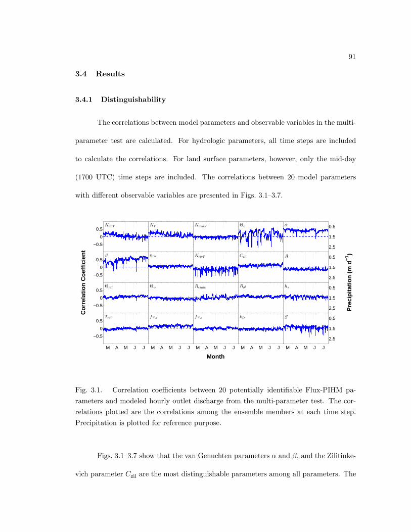
91
3.4 Results
3.4.1 Distinguishability
The correlations between model parameters and observable variables in the multi-
parameter test are calculated. For hydrologic parameters, all time steps are included
to calculate the correlations. For land surface parameters, however, only the mid-day
(1700 UTC) time steps are included. The correlations between 20 model parameters
with different observable variables are presented in Figs. 3.1–3.7.
KinfV
−0.5
0
0.5KV KmacV Θe 0.5
1.5
2.5
α
β
−0.5
0
0.5nriv KrivV Czil 0.5
1.5
2.5
A
Θref
−0.5
0
0.5Θw Rcmin Rgl 0.5
1.5
2.5
hs
Tref
M A M J J
−0.5
0
0.5fxs
M A M J J
fxc
M A M J J
kD
M A M J J
0.5
1.5
2.5
S
M A M J J
Month
Cor
rela
tion
Coe
ffici
ent
Pre
cipi
tatio
n (m
d−1
)
Fig. 3.1. Correlation coefficients between 20 potentially identifiable Flux-PIHM pa-
rameters and modeled hourly outlet discharge from the multi-parameter test. The cor-
relations plotted are the correlations among the ensemble members at each time step.
Precipitation is plotted for reference purpose.
Figs. 3.1–3.7 show that the van Genuchten parameters α and β, and the Zilitinke-
vich parameter Czil are the most distinguishable parameters among all parameters. The

92
KinfV
−0.5
0
0.5KV KmacV Θe 0.5
1.5
2.5
α
β
−0.5
0
0.5nriv KrivV Czil 0.5
1.5
2.5
A
Θref
−0.5
0
0.5Θw Rcmin Rgl 0.5
1.5
2.5
hs
Tref
M A M J J
−0.5
0
0.5fxs
M A M J J
fxc
M A M J J
kD
M A M J J
0.5
1.5
2.5
S
M A M J J
Month
Cor
rela
tion
Coe
ffici
ent
Pre
cipi
tatio
n (m
d−1
)
Fig. 3.2. Same as Fig. 3.1, but for water table depth at RTHnet wells.
KinfV
−0.5
0
0.5KV KmacV Θe 0.5
1.5
2.5
α
β
−0.5
0
0.5nriv KrivV Czil 0.5
1.5
2.5
A
Θref
−0.5
0
0.5Θw Rcmin Rgl 0.5
1.5
2.5
hs
Tref
M A M J J
−0.5
0
0.5fxs
M A M J J
fxc
M A M J J
kD
M A M J J
0.5
1.5
2.5
S
M A M J J
Month
Cor
rela
tion
Coe
ffici
ent
Pre
cipi
tatio
n (m
d−1
)
Fig. 3.3. Same as Fig. 3.1, but for soil water content at RTHnet wells.

93
KinfV
−0.5
0
0.5KV KmacV Θe 0.5
1.5
2.5
α
β
−0.5
0
0.5nriv KrivV Czil 0.5
1.5
2.5
A
Θref
−0.5
0
0.5Θw Rcmin Rgl 0.5
1.5
2.5
hs
Tref
M A M J J
−0.5
0
0.5fxs
M A M J J
fxc
M A M J J
kD
M A M J J
0.5
1.5
2.5
S
M A M J J
Month
Cor
rela
tion
Coe
ffici
ent
Pre
cipi
tatio
n (m
d−1
)
Fig. 3.4. Same as Fig. 3.1, but for mid-day (1700 UTC) skin temperature.
KinfV
−0.5
0
0.5KV KmacV Θe 0.5
1.5
2.5
α
β
−0.5
0
0.5nriv KrivV Czil 0.5
1.5
2.5
A
Θref
−0.5
0
0.5Θw Rcmin Rgl 0.5
1.5
2.5
hs
Tref
M A M J J
−0.5
0
0.5fxs
M A M J J
fxc
M A M J J
kD
M A M J J
0.5
1.5
2.5
S
M A M J J
Month
Cor
rela
tion
Coe
ffici
ent
Pre
cipi
tatio
n (m
d−1
)
Fig. 3.5. Same as Fig. 3.1, but for mid-day (1700 UTC) sensible heat flux.

94
KinfV
−0.5
0
0.5KV KmacV Θe 0.5
1.5
2.5
α
β
−0.5
0
0.5nriv KrivV Czil 0.5
1.5
2.5
A
Θref
−0.5
0
0.5Θw Rcmin Rgl 0.5
1.5
2.5
hs
Tref
M A M J J
−0.5
0
0.5fxs
M A M J J
fxc
M A M J J
kD
M A M J J
0.5
1.5
2.5
S
M A M J J
Month
Cor
rela
tion
Coe
ffici
ent
Pre
cipi
tatio
n (m
d−1
)
Fig. 3.6. Same as Fig. 3.1, but for mid-day (1700 UTC) latent heat flux.
KinfV
−0.5
0
0.5KV KmacV Θe 0.5
1.5
2.5
α
β
−0.5
0
0.5nriv KrivV Czil 0.5
1.5
2.5
A
Θref
−0.5
0
0.5Θw Rcmin Rgl 0.5
1.5
2.5
hs
Tref
M A M J J
−0.5
0
0.5fxs
M A M J J
fxc
M A M J J
kD
M A M J J
0.5
1.5
2.5
S
M A M J J
Month
Cor
rela
tion
Coe
ffici
ent
Pre
cipi
tatio
n (m
d−1
)
Fig. 3.7. Same as Fig. 3.1, but for mid-day transpiration.

95
van Genuchten parameters show high correlations with almost every observable variable,
especially Q, WTD, SWC, LE, and Et. Parameter Czil is most dominant in Tsfc and H
forecast. Among the four observable land surface parameters, variables LE and Et are
more moisture-driven, while Tsfc and H are more energy-driven. Results from Figs. 3.1–
3.7 indicate that the van Genuchten parameters are the most distinguishable parameters
for hydrologic variables and moisture-driven land surface variables, and Czil is the most
distinguishable parameter for energy-driven variables.
At the watershed scale, β shows stronger influences on soil moisture content than
α, which is revealed by the larger correlations between β and domain averaged Tsfc, H,
LE, and Et. But α has much stronger correlation with RTHnet well SWC than β does.
This is caused by the different sensitivities of the soil water retention curve at different
soil saturation ratios in the van Genuchten equation. Fig. 3.8 presents the sensitivity of
soil water retention curve to α and β values.
As shown in Fig. 3.8, soil retention curve is more sensitive to the change of β at
low saturation ratios, but more sensitive to the change of α at high saturation ratios. At
watershed scale, the Shale Hills watershed is a relatively dry watershed, so the change of
β values would produce larger impacts than the change of α. At grid scale, the RTHnet
wells are located near the stream, thus this grid always has a relatively high saturation
ratio (0.6–0.85), in which regime the soil water retention curve is more sensitive to α
values.
Parameters Θe, α and β are the most distinguishable and influential parameters
in the forecast of discharge (Fig. 3.1). The correlations between those parameters and
model discharge are highly time dependent, especially for Θe. During low flow periods,

96
0 0.2 0.4 0.6 0.8 110
−2
100
102
104
θ
h (
m)
α0, β00.63α0, β01.25α0, β01.88α0, β0α0, 1.34β0α0, 1.73β0α0, 2.11β0
Fig. 3.8. Sensitivity of soil water retention curve to α and β values. Calibration
coefficients of α and β are evenly distributed in their corresponding plausible ranges.

97
Θe is positively correlated with discharge, while for discharge peaks, Θe is negatively
correlated with discharge rate. The role of Θe is defining the available water storage of
soil. Discharge at low flow periods mostly comes from lateral groundwater flow. Larger
Θe leads to more water storage, and thus larger lateral groundwater flow at low flow
periods. In contrast peak flow mostly consists of surface runoff. Smaller Θe leads to less
water storage, and thus faster saturation and larger surface runoff. As a result, Θe is
positively correlated with discharge during low flow periods, but negatively correlated
with discharge at peak flows. Parameter α and β consistently show high correlations with
discharge, except at those discharge peaks. Parameter S shows considerable correlation
with discharge at discharge peaks, but low correlation for most of the time.
For WTD and SWC (Figs. 3.2 and 3.3), α and β are the most highly correlated pa-
rameters, but the correlations decrease at wet periods, suggesting that the peaks in SWC
and drops in WTD might be controlled by the atmospheric forcing, e.g., precipitation,
and other model parameters. Parameters KinfV and KrivV also show high correlations
with WTD during wet periods, because of their roles in vertical water transport. The
time series of correlation coefficients for discharge and WTD are very similar (Figs. 3.1
and 3.2). For each parameter, the two time series for discharge and WTD are almost
symmetric with respect to the axis of zero-correlation, although time series for discharge
has more high-frequency changes (Figs. 3.1 and 3.2). Flux-PIHM simulation shows that
at the Shale Hills watershed, 83% of total discharge is attributed to lateral groundwater
flow in year 2009. The change of water table depth near the stream is therefore highly
correlated with the change of discharge rate.

98
The parameter Czil shows a very high correlation (nearly 1.0) with the surface
skin temperature, while the distinguishability of other parameters are relatively low
(Fig. 3.4). Because of the explicit role of surface exchange coefficients in sensible heat
flux formulation [Eq. (2.26)], Czil shows high correlation with the sensible heat flux as
well (Fig. 3.5). The influences of α and β on Tsfc and H get increasingly important
from spring to summer (Figs. 3.4 and 3.5). The influences of those two parameters on
sensible heat flux are indirect, and are made by affecting evapotranspiration and thus
surface energy balance. When leaves are not out yet in spring, evapotranspiration rate
is small, thus the influences of α and β on surface energy balance are weak. In summer,
when evapotranspiration is strong, the influences of α and β on surface energy balance
get stronger.
Both subsurface and land surface parameters show strong impacts on latent heat
flux predictions, and their roles change with season. Impacts of α and β on latent heat
flux are stronger than on sensible heat flux, because their influences are more direct on
moisture-driven variables (Fig. 3.6). The correlation between those two parameters and
LE also gets stronger in summer than in spring. Impacts of α and β are stronger in dry
periods (when canopy is dry) than in wet periods (when canopy is wet). In wet periods,
influences of Czil and S are significant. The actual evapotranspiration is a fraction of
potential evapotranspiration, and can be written as
E = f(Θ, Ta, S ↓,∆q, · · · )Ep, (3.7)

99
where Ep is the potential evapotranspiration, and f is a function of soil moisture Θ, air
temperature Ta, solar radiation S ↓, water vapor deficit ∆q, etc. The parameter Czil
affects Ep, while α and β influence the function f . Different sensitivities between dry and
wet periods suggest that during wet periods, evapotranspiration is mostly determined by
potential evapotranspiration, whereas during dry periods, evapotranspiration is mostly
constrained by the function f . The parameter S also has strong influence when canopy
is wet. Parameter fxs which controls the rate of soil evaporation shows consistent
correlation around −0.25 with latent heat flux.
Effects of α and β on transpiration are similar to their effects on latent heat
flux (Fig. 3.7). Because canopy evaporation and transpiration are competing processes,
parameters kD and S which control the canopy evaporation are highly distinguishable
when canopy is wet. The parameter Rc min shows consistent correlation around −0.25
with transpiration. The correlation between Tref and transpiration reaches about −0.5
in spring, but is close to 0 in summer. The seasonal change of the correlation between
Tref and transpiration suggests that spring transpiration is strongly constrained by air
temperature stress on canopy resistance [Eq. (2.24)], but the constraint gets weaker in
summer.
While Figs. 3.1–3.7 examine the correlation between model parameters and ob-
servable variables at each time step, the overall distinguishability during the whole ex-
periment period needs to be quantified. Figs. 3.1–3.7 show that the correlation between
model parameters and observable variables is highly seasonally dependent, and event
based. To evaluate the overall correlation within the experiment period, a root mean

100
squared correlation coefficient (RMSC) is calculated as:
RMSC =
√
∑
t
(ρt)2, (3.8)
where ρt is the correlation coefficient between model parameter and observable variables
at time step t. The RMSCs between all parameters and observable variables are presented
in Fig. 3.9.
Q
WTD
SWC
Tsfc
H
LE
Et
Obs
erva
ble
Var
iabl
e
KinfV KV KmacV Θe α β nriv KrivV Czil A Θref Θw Rcmin Rgl hs Tref fxs fxc kD S
Parameter
0
0.1
0.2
0.3
0.4
0.5
0.6
0.7
0.8
0.9
1
Fig. 3.9. RMSC between twenty potentially identifiable Flux-PIHM parameters and
different observable variables. The horizontal (vertical) white lines divide observable
variables (parameters) into hydrologic and land surface variables (parameters).
Fig. 3.9 shows that parameters α, β, and Czil all have RMSCs larger than 0.5 with
one or more observable variables. Effects of those parameters are highly distinguishable
in the multi-parameter test, which suggests those parameters are the most influential

101
parameters in Flux-PIHM, and might also be highly observable. Low distinguishability,
however, is not necessarily equivalent to low observability. Because of the interaction of
model parameters, the effects of some parameters might be compensated by the effects of
other parameters, as suggested by model equifinality (Beven 1993). Thus, observability
needs to be tested with single parameter tests.
There are ten parameters, five hydrologic parameters and five land surface pa-
rameters, having RMSCs greater than 0.2 with at least one of the observable variables.
They are:
(1) KV (0.21 with H),
(2) Θe (0.33 with Q, and 0.24 with WTD),
(3) α (0.41 with Q, 0.39 with WTD, 0.82 with SWC, 0.20 with Tsfc, 0.40 with LE,
and 0.41 with Et),
(4) β (0.50 with Q, 0.41 with WTD, 0.36 with H, 0.62 with LE, and 0.60 with Et),
(5) KrivV (0.22 with WTD),
(6) Czil (0.92 with Tsfc, 0.79 with H, 0.35 with LE, and 0.24 with Et),
(7) Rc min (0.21 with Et),
(8) fxs (0.21 with Tsfc and 0.22 with LE),
(9) kD (0.20 with Et), and
(10) S (0.26 with H and 0.26 with Et).

102
Those parameters with relatively high distinguishability qualify for single parameter test
to further examine their observability and simplicity.
3.4.2 Observability
To test the observability of the model parameters, a group of 10 Flux-PIHM model
runs are performed for every qualified parameter, which results in a total of 100 Flux-
PIHM model runs. The RMSDs of observable variables at each time step are calculated.
Those time series of RMSDs for different observable variables from different ensemble
groups are used to compare the observability of parameters. The comparisons for RMSDs
of different observable variables are shown in Figs. 3.10–3.16.
0
0.5
1
1.5
2
2.5
3
Pre
cipi
tatio
n (m
d−1
)
RM
SD
of
Q (
m3 d
−1)
MonthM A M J J
0
100
200
300
400
500
KV
ΘeαβKrivV
Czil
Rcmin
fxs
kDS20 Jun 22 Jun
0
500
1000
1500
Fig. 3.10. RMSDs of discharge simulations in single parameter tests. Grey lines indicate
strength of precipitation, which is plotted for reference purpose. The inset presents the
RMSDs at the discharge peak between 20 June and 22 June 2009.

103
.
0
0.5
1
1.5
2
2.5
3
Pre
cipi
tatio
n (m
d−1
)
RM
SD
of W
TD
(m
)
MonthM A M J J
0
0.05
0.1
0.15
0.2
0.25
0.3
0.35
0.4
KV
ΘeαβKrivV
Czil
Rcmin
fxs
kDS
Fig. 3.11. Same as Fig. 3.10, but for WTD.
As expected, parameters with high distinguishability all show high observability in
corresponding observable variables, indicated by the relatively high RMSDs in predicted
observable variables (Figs. 3.10–3.16). Most of the information from those figures can be
deduced from examinations of the correlations from multi-parameter test, except that
some parameters with low distinguishability show considerable observability in some
of the observable variables. For example, the influence of Czil on model discharge is
not distinguishable from other parameters in the multi-parameter test (Fig. 3.1) , but
Czil produces large RMSDs in model discharge in the single parameter test (Fig. 3.10).
This can be explained by model equifinality (Beven 1993)—the influence of Czil on model

104
0
0.5
1
1.5
2
2.5
3
Pre
cipi
tatio
n (m
d−1
)
RM
SD
of S
WC
(m
3 m−3
)
MonthM A M J J
0
0.01
0.02
0.03
0.04
0.05
0.06
0.07
KV
ΘeαβKrivV
Czil
Rcmin
fxs
kDS
Fig. 3.12. Same as Fig. 3.10, but for SWC.
0
0.5
1
1.5
2
2.5
3
Pre
cipi
tatio
n (m
d−1
)
RM
SD
of
Tsf
c (
° C)
MonthM A M J J
0
5
10
15
20
KV
ΘeαβKrivV
Czil
Rcmin
fxs
kDS
Fig. 3.13. Same as Fig. 3.10, but for mid-day (1700 UTC) Tsfc.

105
0
0.5
1
1.5
2
2.5
3
Pre
cipi
tatio
n (m
d−1
)
RM
SD
of
H (
W m
−2)
MonthM A M J J
0
50
100
150
KV
ΘeαβKrivV
Czil
Rcmin
fxs
kDS
Fig. 3.14. Same as Fig. 3.10, but for mid-day (1700 UTC) H.
0
0.5
1
1.5
2
2.5
3
Pre
cipi
tatio
n (m
d−1
)
RM
SD
of
LE
(W
m−2
)
MonthM A M J J
0
50
100
150
KV
ΘeαβKrivV
Czil
Rcmin
fxs
kDS
Fig. 3.15. Same as Fig. 3.10, but for mid-day (1700 UTC) LE.

106
0
0.5
1
1.5
2
2.5
3
Pre
cipi
tatio
n (m
d−1
)
RM
SD
of
Et (
mm
d−1
)
MonthM A M J J
0
0.5
1
1.5
2
2.5
3
3.5
4
KV
ΘeαβKrivV
Czil
Rcmin
fxs
kDS
Fig. 3.16. Same as Fig. 3.10, but for mid-day (1700 UTC) Et.
discharge is compensated by influences of other model parameters in the multi-parameter
test.
While hydrologic parameters α and β show strong impacts on land surface vari-
ables (Figs. 3.13–3.16), land surface parameters, especially Czil and Rc min, also show
considerable impacts on hydrologic variables (Figs. 3.10–3.12). In the land surface mod-
ule, parameters Czil and Rc min influence evapotranspiration the most (Figs. 3.15 and
3.16). Evapotranspiration extracts soil water and groundwater within the root zone and
changes the soil moisture and the water table depth. Although in dry periods (low flow
periods), the influences of land surface parameters on hydrologic variables are not as
strong as α and β, those influences change the system response to strong precipitation.
During peak flow periods, the RMSDs in Q, WTD and SWC produced by Czil and
Rc min are comparable to those produced by α and β (Fig. 3.10). Especially for the peak
107
event in July, Czil produces the largest RMSD in discharge peak, and influences model
discharge the most because this event happens after an extended relatively dry period.
It implies that the evapotranspiration forecasting before a strong precipitation event is
critical for the accurate forecasting of discharge peaks. This agrees with the finding of
Kampf (2006), who stated that the accuracy of discharge forecast depends on accurate
simulations of evapotranspiration.
As shown in Fig. 3.9, parameters Θe, α, and β are the most influential parameters
on model discharge. RMSDs are large at discharge peaks (Fig. 3.10). Effect of Θe is the
most significant during discharge peaks, but relatively weak during low flow conditions.
The parameter β shows high observability consistently, during both peak flow and low
flow periods. For the highest peak in June 2009, RMSDs of discharge simulations using
different parameters reach as high as 1400 m3 d−1, which shows the accuracy of hydro-
logic model is severely constrained by parameter uncertainties. Besides Czil, land surface
parameters Rc min and fxs also show considerable observability in discharge simulations.
In spring, when leaves are not out, the influences of fxs (soil evaporation) is stronger
than Rc min (transpiration). In summer, when transpiration process dominates the total
evapotranspiration, Rc min is more influential than fxs.
The impacts of model parameters on WTD and SWC at RTHnet wells are similar,
except that α is more influential than β in SWC simulations (Figs. 3.11 and 3.12). From
spring to summer, the impacts of land surface parameters get stronger on WTD and
SWC. Because of their roles in groundwater recharge, KV and KrivV also show relatively
strong influences on the simulations of WTD and SWC.

108
The impact of Czil on mid-day surface skin temperature is far more significant
than any other parameter (Fig. 3.13). The RMSDs caused by different Czil reach 20 ◦C,
while the RMSDs caused by other parameters are always below 5 ◦C. RMSDs of Tsfc are
larger in summer and in dry periods, when Tsfc is relatively higher; and smaller in spring
and in wet periods, when Tsfc is relatively lower.
The impact of Czil on mid-day sensible heat flux is the most significant in spring
(Fig. 3.14). But the RMSDs of sensible heat flux caused by different Czil values decrease
in summer because the magnitude of sensible heat flux drops. In contrast, observability of
hydrologic parameters increases from spring to summer. This is because the Bowen ratio
is small in summer and latent heat flux dominates the surface energy balance. Hydrologic
parameters then have stronger influences on sensible heat flux via their impacts on
evapotranspiration.
For mid-day latent heat flux and transpiration, RMSDs caused by different pa-
rameters are small in spring, when latent heat flux is small, and large in summer, when
latent heat flux is large (Fig. 3.15). Hydrologic parameters α and β, and land surface
parameters Czil and Rc min are the most influential parameters, especially β. The pa-
rameter S also shows relatively high observability on latent heat flux and transpiration
during wet periods, when canopy is wet and canopy evaporation occurs.
Three hydrologic parameters and three land surface parameters are chosen for
simplicity testing as a result of the distinguishability and observability tests. The in-
clusion of hydrologic parameter α and β is straightforward. The effective porosity, Θe,
is chosen as the other hydrologic parameter because of its strong impact of discharge
peaks, the accurate forecast of which is a critical criterion of hydrologic models. Selection
109
of land surface parameter Czil is also straightforward. The parameter Rc min is chosen
because it shows high observability in both hydrologic and land surface variables, and
also has reasonable distinguishability. The other land surface parameter selected is S,
because of its effect on evapotranspiration and discharge during wet periods.
3.4.3 Simplicity
For those six parameters with high distinguishability and observability, their sim-
plicity is examined. Both multi-parameter test results and single test results are used. To
test the simplicity, the observable variables from all model runs are plotted as functions
of the model parameters. One observable variable is selected for each parameter in the
simplicity examination. For parameters Θe and β, the variable Q is selected; for α, SWC
is picked; for Czil, Tsfc is examined; and for Rc min and S, Et is plotted. Examinations
of distinguishability and observability imply that the relationship between variables and
parameters could be different in wet and dry periods, different in high flow and low
flow conditions, and different for wet and dry canopy. Therefore, simplicity needs to be
examined for both wet and dry periods. Two mid-day time steps are chosen to represent
wet and dry periods. The first time chosen is 1700 UTC 20 June 2009, which represents
the wet period, high flow condition, and wet canopy. It has been almost continuously
raining from 1300 UTC 17 June to 0000 UTC 21 June. The observed highest discharge
peak during the whole simulation periods occurs around 1800 UTC 21 June. Because
of the continuous precipitation, canopy is wet at this time step. The second time step
chosen is 1700 UTC 11 July 2009, which represents the dry period, low flow condition,
and dry canopy. The period from the beginning of July to 11 July is relatively dry. For

110
the 48 hours prior to 1700 UTC 11 July, there has been no precipitation, and the canopy
is dry. Relations between different observable variables and different model parameters
are presented in Figs 3.17 and 3.18.
0.4 0.6 0.8 10
1000
2000
3000
4000
5000
Θe
Q (
m3 d
−1)
0 1 20.1
0.2
0.3
0.4
0.5
α
SW
C (
m3 m
−3)
1 1.5 2 2.50
1000
2000
3000
4000
5000
β
Q (
m3 d
−1)
−1 0 120
25
30
35
40
lgCzil
Tsf
c (
° C)
0.4 0.6 0.8 10
0.2
0.4
0.6
0.8
Rcmin
Et (
mm
d−1
)
0 2 40
0.2
0.4
0.6
0.8
1
S
Et (
mm
d−1
)
Fig. 3.17. Flux-PIHM observable variables at 2000 UTC 20 June 2009 plotted as
functions of model parameters. Blue dots are from the multi-parameter test and red
dots are from the single parameter tests.
Figs. 3.17 and 3.18 show that for both wet and dry periods, those six parameters
show high simplicity in their corresponding observable variables. Except for Q-β in the
wet period and Et-S in the dry period, the other observable variables change mono-
tonically with the change of parameter values in both wet and dry periods. The Q-β
relationship at 1700 UTC 20 June is not clear. The examination of correlation between
β and Q in multi-parameter test also shows low correlation at this time step (Fig. 3.1).
When the calibration coefficient of β varies between 1.0–1.5, discharge at this time step

111
0.4 0.6 0.8 10
50
100
150
Θe
Q (
m3 d
−1)
0 1 20
0.1
0.2
0.3
0.4
α
SW
C (
m3 m
−3)
1 1.5 2 2.50
50
100
150
β
Q (
m3 d
−1)
−1 0 125
30
35
40
45
lgCzil
Tsf
c (
° C)
0.4 0.6 0.8 10
1
2
3
4
Rcmin
Et (
mm
d−1
)
0 2 40
1
2
3
4
S
Et (
mm
d−1
)
Fig. 3.18. Same as Fig. 3.17, but at 1700 UTC 11 July 2009.
increases with the increase of β. And when calibration coefficient of β varies between
1.5–2.3, discharge at this time step is not affected by β. Discharge at this time step
decreases when calibration coefficient of β is greater than 2.3. The low simplicity of
β in model discharge at this time step suggests that finding an optimal β value using
discharge forecast at this time step might be difficult. Luckily, at the selected dry time
step, discharge increases monotonically with the increase of β. Given that β shows high
observability and distinguishability in multiple observable variables and given the high
simplicity at low flow period, it is feasible to find an optimal value for β. As for Et-S
at 1700 UTC 11 July, transpiration is not affected by S (Fig. 3.18). This is because
the canopy is dry and S is not in effect. At the wet time step, however, S shows good
simplicity in Et (Fig. 3.17).

112
At the peak flow period, Q decreases monotonically and smoothly with the in-
crease of Θe (Fig. 3.17). At the low flow period, Q increases with the increase of Θe
(Fig. 3.18). The different effects of Θe in peak flow and low flow are also found in the
correlation between Q and Θe in the multi-parameter test (Fig. 3.1), which shows Q and
Θe are negatively correlated at peak flows but positively correlated during low flow pe-
riods. For the other parameters, effects in those corresponding observable variables are
similar in both dry and wet periods. The chosen observable variables vary monotonically
and smoothly with the change of those parameter values.
Examinations of parameter distinguishability, observability, and simplicity show
that Flux-PIHM hydrologic parameters Θe, α, and β, and land surface parameters Czil,
Rc min, and S have relatively high identifiability. In the following chapters, those six
parameters are chosen for parameter estimation using EnKF.
It is important to point out that the examinations of identifiability are made in the
context of the selected parameter range and parameter distribution. It is highly possible
that the identifiability of parameters become different if different ranges are selected,
especially distinguishability and observability. The reason for hydrologic parameters
showing stronger distinguishability and observability than land surface parameters might
be that hydrologic parameters are more weakly constrained than land surface parameters.
3.5 Discussions and conclusions
Parameter sensitivity tests are a vital step towards successful parameter estima-
tion.In this chapter, a parameter sensitivity test for Flux-PIHM model parameters is
performed under the framework provided by Nielsen-Gammon et al. (2010). Among all

113
test methods, the evaluation of the correlation between model parameters and observable
variables is the most critical test. The correlation coefficients directly indicate param-
eter distinguishability. Results show that parameters with high distinguishability also
have high observability, because their impacts on the system cannot be compensated by
the effects from other parameters. Moreover, because correlation coefficient represents
linear dependence, a high correlation coefficient also suggests highly linear dependence,
and hence simplicity.
Model sensitivity test reveals that the land surface hydrologic model is very sensi-
tive to parameter values, especially parameter values of α, β, and Czil. For the discharge
peak in June 2009, the observed discharge rate is 1860 m3 d−1, but the single parameter
test RMSDs of the discharge simulations can be as large as 1400 m3 d−1 for some model
parameters. The RMSDs of mid-day surface skin temperature simulations are as large
as 20 ◦C in the single parameter test for Czil. Parameter uncertainties produce large
model uncertainties in hydrologic and land surface simulations.
Examinations of parameter distinguishability and observability indicate that the
land surface and the subsurface are coupled systems in Flux-PIHM. In Flux-PIHM,
the subsurface and land surface are linked together by exchanging soil moisture and
evapotranspiration information. The subsurface (hydrologic) component provides soil
moisture information for the land surface component, while the land surface component
provides evapotranspiration rate for the subsurface component. Hydrologic parameters,
especially the van Genuchten parameters, have significant influence on land surface sim-
ulations through their impacts on soil moisture simulations. At the same time, land
surface parameters, especially Czil and Rc min have considerable impacts on discharge,

114
groundwater level, and soil moisture simulations through their influences on evapotran-
spiration. In summer, the observable hydrologic variable RMSDs caused by land surface
parameters, and the observable land surface variable RMSDs caused by hydrologic pa-
rameters are higher than in spring. It suggests that the interaction between the land
surface and the subsurface is especially strong in summer, when evapotranspiration is
more active than in other seasons. The interaction between the subsurface and the land
surface suggests that accurate forecasting of hydrologic states cannot be made without
reasonable descriptions of land surface, and vice versa. It justifies the need for a coupled
land surface hydrologic model.
Examination of parameter distinguishability shows that some parameters with
high observability in a certain observable variable do not show high distinguishability for
the corresponding observable variable in multi-parameter test. For example, parameter
Czil exhibits high observability in discharge in the single parameter test (Fig. 3.10), but
shows low distinguishability in discharge in the multi-parameter test (Fig. 3.1). This is
because the impacts of those parameters are compensated by the effects of other model
parameters. Model equifinality (Beven 1993) indicates that the parameter interaction
within Flux-PIHM is strong. Parameter estimation is essentially an inverse problem,
which converts observed variables into information about model parameters (Moradkhani
and Sorooshian 2008). The equifinality and parameter interaction add extra difficulties
for parameter estimation. The more observed variables we have, the better chance there
is to overcome the difficulties brought by equifinality. Therefore, using multiple types of
observations for calibration could be important for parameter estimation.
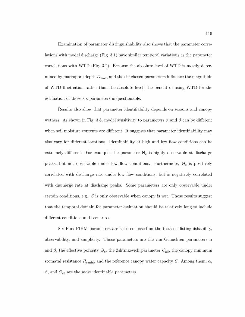
115
Examination of parameter distinguishability also shows that the parameter corre-
lations with model discharge (Fig. 3.1) have similar temporal variations as the parameter
correlations with WTD (Fig. 3.2). Because the absolute level of WTD is mostly deter-
mined by macropore depth Dmac, and the six chosen parameters influence the magnitude
of WTD fluctuation rather than the absolute level, the benefit of using WTD for the
estimation of those six parameters is questionable.
Results also show that parameter identifiability depends on seasons and canopy
wetness. As shown in Fig. 3.8, model sensitivity to parameters α and β can be different
when soil moisture contents are different. It suggests that parameter identifiability may
also vary for different locations. Identifiability at high and low flow conditions can be
extremely different. For example, the parameter Θe is highly observable at discharge
peaks, but not observable under low flow conditions. Furthermore, Θe is positively
correlated with discharge rate under low flow conditions, but is negatively correlated
with discharge rate at discharge peaks. Some parameters are only observable under
certain conditions, e.g., S is only observable when canopy is wet. Those results suggest
that the temporal domain for parameter estimation should be relatively long to include
different conditions and scenarios.
Six Flux-PIHM parameters are selected based on the tests of distinguishability,
observability, and simplicity. Those parameters are the van Genuchten parameters α
and β, the effective porosity Θe, the Zilitinkevich parameter Czil, the canopy minimum
stomatal resistance Rc min, and the reference canopy water capacity S. Among them, α,
β, and Czil are the most identifiable parameters.

116
Chapter 4
Flux-PIHM Parameter Estimation
Using Ensemble Kalman Filter:
A Synthetic Experiment
4.1 Introduction
Land surface models (LSMs) and hydrologic models are important tools for the
forecasting and study of land surface and hydrologic processes. LSMs simulate the ex-
change of mass, momentum and energy between the land surface and the atmosphere.
They play important roles in weather and climate forecasting, and provide necessary
lower boundary conditions for atmospheric models. Hydrologic models simulate hydro-
logic system responses to incoming precipitation. They are essential tools to enhance
the understanding of hydrological processes and to simulate and predict flood/drought
events for better decision-making. Both LSMs and hydrologic models are highly param-
eterized models. Model structures are complex and the number of involved parameters is
often large. The accuracy of LSMs and hydrologic models is limited by the uncertainties
in model parameters. Parameter estimation of LSMs and hydrologic models has been
the focus of many studies (e.g., Gupta et al. 1999; Xia et al. 2002; Jackson et al. 2003).
Especially for hydrologic models, the uncertainties in model parameters are the
main source of uncertainties (Moradkhani and Sorooshian 2008). To reduce the un-
certainty in model parameters and for hydrologic model to yield the observed system

117
response of a specific watershed, hydrologic model parameters always need to be cali-
brated. For hydrologic models, the physical parameter values in actual field condition
might be substantially different from those measured in laboratory; the range of variation
in parameter values spans orders of magnitude (Bras 1990). Some physical parameters
have considerable spatial heterogeneity which weakens the representativity of measure-
ments. Consequently, parameter uncertainties in those models are often large. Those
difficulties make model calibration the most demanding and time-consuming task in
applying hydrologic models.
In the past few decades, many hydrologic model calibration methods have been
proposed and studied. A basic calibration approach is the “trial and error” method,
or manual calibration. In manual calibration, model performances are visually in-
spected, and then model parameter values are tuned to minimize the differences between
model and observations, based on human judgment (Boyle et al. 2000; Moradkhani and
Sorooshian 2008). This method is very labor-intensive and time-consuming. Manual cal-
ibration of physically-based hydrologic models can be extremely difficult due to the high
dimensionality of the parameter space and the strong interaction between model param-
eters. Those difficulties motivated the development of automatic calibration methods.
Generally, there are two strategies for automatic calibration: batch (iterative) cal-
ibration and sequential (recursive) calibration. Batch calibration aims to minimize the
predefined objective functions by repeatedly searching in the parameter space and eval-
uating long period model performances (e.g., Ibbitt 1970; Johnston and Pilgrim 1976;
Pickup 1977; Gupta and Sorooshian 1985; Duan et al. 1992; Sorooshian et al. 1993;
Franchini 1996; Wagener et al. 2003; Kollat and Reed 2006). Batch calibration requires

118
previously collected historical data for model evaluation and is thus restricted to offline
applications. Batch calibration has limited flexibility in dealing with the possible tempo-
ral evolution of model parameters (Moradkhani et al. 2005; Moradkhani and Sorooshian
2008).
Sequential calibration methods could take advantage of measurements whenever
they are available and are thus useful in both online and offline applications. Sequential
calibration also explicitly addresses uncertainties in input data and model structures,
and has more flexibility of dealing with time-variant parameters, compared with batch
calibration methods. Among all filter and smoother techniques for sequential calibration,
different forms of Kalman filter are the most widely used algorithms. The first attempts
of parameter estimation using standard Kalman filter (KF; Kalman 1960) dated back
to 1970s (e.g., Todini et al. 1976; Kitanidis and Bras 1980a,b). But this method is
only limited to linear dynamic systems. Extended Kalman Filter (EKF) can be used
for nonlinear dynamic systems but tend to be unstable when the nonlinearities in the
systems are strong. EKF is based on linearization of model by neglecting the higher
order derivatives, which could lead to unstable results or even divergence (Evensen 1994;
Reichle et al. 2002a). Because model errors are estimated by propagating model covari-
ance matrix forward in time, EKF also has large computational demand, especially for
high dimensional state vector, which makes it almost impractical for spatially distributed
models (Reichle et al. 2002b).
Because of the high computational demands of physically-based hydrologic model,
it is very difficult to use batch calibration methods for calibration (Tang et al. 2006).

119
Their high dimensional parameter space and high nonlinearity pose difficulties for se-
quential methods as well. The recently proposed ensemble Kalman filter (EnKF; Evensen
1994) provides a promising approach for distributed physically-based hydrologic model
auto calibration. EnKF has been widely used for parameter estimation in recent years
(e.g., Aksoy et al. 2006; Hu et al. 2010; Cammalleri and Ciraolo 2012). EnKF is not
only useful in improving variable and parameter estimations, but could also provide
uncertainty estimations of variables and parameters. Compared with other forms of
Kalman filters, EnKF is capable of handling strongly nonlinear dynamics, high dimen-
sional state vectors, and to some degree non-Gaussianity. It also has a simple conceptual
formulation, relative ease of implementation, and affordable computational requirements
(Evensen 2003). Moradkhani et al. (2005) applied EnKF onto a lumped conceptual
rainfall-runoff (R-R) model to estimate the values of five model parameters using real
observations. The obtained parameter set from EnKF is similar with the results from
batch calibration. The ensemble discharge forecast also agrees well with observations.
Xie and Zhang (2010) applied EnKF onto a spatially-distributed conceptual hydrologic
model to estimate the values of a spatially-distributed parameter in different hydrologic
response units (HRUs). In synthetic data experiments, at most of HRUs, the estimated
values of the parameter are very close to the true values when synthetic discharge obser-
vations are assimilated. To a broader extent, there are also studies implementing EnKF
in groundwater models to estimate model parameters such as hydraulic conductivities
(e.g., Chen and Zhang 2006; Liu et al. 2008). Although EnKF has been proved effective
for lumped and distributed conceptual models, the effectiveness of EnKF in parameter

120
estimation for physically-based hydrologic models, or land surface hydrologic models is
still untested.
Data assimilation for fully-coupled physically-based hydrologic models using EnKF
will be difficult because of the high dimensionality of the joint vector of state variables
and model parameters. Compared with conceptual models, physically-based models gen-
erally have more model parameters, more model grids, and more state variables at each
grid. A relatively large number of model grids with more state variables and model
parameters results in a high dimensional joint vector of states and parameters, which
makes the implementation of EnKF difficult and increases computational cost.
Physically-based models also require a long adjustment period after each assimi-
lation cycle. In physically-based models, model formulations and parameters define the
equilibrium among model state variables in the system. The equilibrium of the sys-
tem not only include the equilibrium between surface water, saturated water storage,
and unsaturated water storage within a model grid, but also the equilibrium between
different grids. The update of state variables and parameters via EnKF could break
the equilibrium in the system (Pan and Wood 2006) which requires a time period for
adjustment. The equilibrium needs to be reestablished through the exchange of water
among different water components in a single water grid, e.g., infiltration, groundwater
recharge, and root zone uptake, and through the exchange of water among different grids,
e.g., horizontal groundwater flow. The excess water is “squeezed” out from the model
domain like being squeezed out from a sponge, and would eventually flow into the river
channel and leave the model domain as outlet discharge. During this adjustment period,
the covariance matrix between the model predictions and the joint vector of states and

121
parameters is contaminated by this “sponge effect”. If the assimilation interval is shorter
than the adjustment period, EnKF would update state variables and model parameters
using a contaminated covariance matrix which could degrade EnKF analysis. A long as-
similation interval, however, means fewer observations could be assimilated, which could
also affect model performances due to the lack of observations. Therefore, finding the
optimal assimilation interval is important, especially when observations are scarce.
Identifying critical observations for model parameter estimation is important for
model calibration, for enhancing the understanding of the inverse problem of parameter
estimation, and for the observational system design at experimental sites. Classically,
only discharge data are used for R-R model data assimilation, while soil moisture and
surface brightness data are used for LSMs (e.g., Houser et al. 1998; Crow and Wood
2003; Pauwels and De Lannoy 2006; Pan and Wood 2006; Clark et al. 2008). Some
recent studies have assimilated multiple types of observations into hydrologic model. It
has been shown that the assimilation of soil moisture in addition to discharge into R-R
model improves the forecast of discharge (e.g., Oudin et al. 2003; Aubert et al. 2003;
Francois et al. 2003; Camporese et al. 2009; Lee et al. 2011), especially during flood events
(Aubert et al. 2003). Xie and Zhang (2010) also found that in synthetic experiments,
the assimilation of soil moisture in addition to discharge improves the estimation of
model parameters. Schuurmans et al. (2003) improved the simulated spatial pattern of
evapotranspiration hence water balance by assimilating remotely sensed latent heat flux
into a hydrologic model.
This chapter presents the first attempt of multiple parameter estimation of a
fully-coupled physically-based land surface hydrologic model (Flux-PIHM) using EnKF.

122
The hydrologic land surface model used in this study is Flux-PIHM, which is based
on the Penn State Integrated Hydrologic Model (PIHM; Qu 2004; Qu and Duffy 2007;
Kumar 2009) and the land surface scheme from the Noah LSM (Chen and Dudhia 2001;
Ek et al. 2003). Six Flux-PIHM parameters, including three hydrologic parameters
and three land surface parameters are estimated using EnKF. Those parameters are
selected through a model parameter sensitivity test (Chapter 3). Synthetic experiments
are executed to test the capability of EnKF in multiple parameter estimation and to
find the optimal assimilation interval for data assimilation. In synthetic experiments,
the synthetic observations are obtained by adding noise to a “truth” Flux-PIHM run
with a specific parameter set. The forecast model has perfect forcing data, perfect soil
and vegetation maps, perfect topography data, and perfect model structures. This is
important for the design of the data assimilation system because the results will not be
contaminated by forcing data errors, input static data errors, model structures errors,
etc.
Integrated synthetic observations of discharge, water table depth, soil moisture
content, land surface temperature, sensible and latent heat fluxes, and canopy transpi-
ration, and some subsets of those observations are assimilated to identify the critical
observations for parameter estimation. The model is implemented at the Shale Hills
watershed in central Pennsylvania, where the broad array of observations provides the
possibility for a future real-data test.

123
4.2 Development of the Flux-PIHM data assimilation system
4.2.1 EnKF
After its introduction by Evensen (1994), EnKF has been widely used in at-
mospheric, geographic and oceanic sciences. It was first developed for dynamic state
estimation to improve initial conditions for numerical forecasts, and was later applied
to model parameter estimation. A schematic illustration of hydrologic model parameter
estimation using EnKF is presented in Fig. 4.1.
0.5 1 1.5 2 2.50
50
100
150
200
250
β
Dis
char
ge (
m3 d
−1)
PriorPosterior
Fig. 4.1. Schematic description of EnKF parameter update. The blue dots represent
prior values of model discharge and calibration coefficients of parameter β. The red dots
represent posterior values updated by EnKF. The black arrow indicates the observation
assimilated into the system. Blue and red arrows indicate the prior and posterior means.

124
In this example, the observation of outlet discharge is used to optimize the Flux-
PIHM parameter β. The figure shows that the forecasted discharge rates and the pa-
rameter β values are positively correlated. The spread in forecast discharge rates and
parameter β values represents the forecast uncertainty and parameter uncertainty, re-
spectively. In the EnKF analysis step, an observation of 28.5 m3 d−1 is assimilated into
the system. The best estimate of model discharge given by EnKF is between the ensem-
ble forecast mean and the observation (indicated by the red arrow on discharge axis),
and weighs both the uncertainties of the ensemble forecast and the observation. Be-
cause discharge and β are positively correlated and the ensemble forecast overestimates
discharge, the posterior mean β value (indicated by the red arrow on β axis) given by
EnKF analysis is smaller than the prior mean value. It is also shown that the spread
of posterior is smaller than the spread of prior in both discharge and β, which indicates
that EnKF effectively decreases forecast uncertainties and parameter uncertainties.
The EnKF formulation used by Snyder and Zhang (2003) is adopted in this study.
In EnKF, the posterior estimate, i.e., analysis is given by
xa = xf + K(
y − Hxf)
, (4.1a)
and the analysis error covariance is given by
Pa = (I − KH)Pf , (4.1b)

125
where xf is the prior estimate, Pf is the forecast background error covariance, y is
the observation vector, H is the observation operator which maps state variables onto
observations, I is the identity matrix, and K is the Kalman gain matrix defined as
K = PfHT(
HPfHT + R)
−1, (4.2)
where R is the observation error covariance.
The state augmentation approach, which has been tested in many studies (e.g.,
Annan 2005; Aksoy et al. 2006; Hu et al. 2010; Xie and Zhang 2010), is adopted for
parameter estimation. In state augmentation approach, parameters and state variables
are concatenated into a joint state vector x, and are updated simultaneously by EnKF.
In order to avoid filter divergence (Anderson and Anderson 1999), the covariance
relaxation method of Zhang et al. (2004) is used. After the state variables and model pa-
rameters are updated by EnKF, the analysis error covariance is inflated using a weighted
average between the prior perturbation and the posterior perturbation:
(xanew
)′ = (1 − a) (xa)′ + a(xf )′, (4.3)
where a is a weighting coefficient. In this study, a is set to be 0.5 as in the study
by Zhang et al. (2006). Because model parameters are not dynamical variables, the
values of parameters remain constant in each forecast step. Therefore, the adoption
of covariance relaxation is not sufficient to avoid filter divergence caused by constantly
decreasing covariance of model parameters. The conditional covariance inflation method

126
Aksoy et al. (2006) is applied onto model parameters in addition to Eq. (4.3): posterior
standard deviation σ of model parameters is inflated back to a predefined threshold when
the standard deviation is smaller than the threshold. The threshold is chosen as 0.25σ0
as in Aksoy et al. (2006), where σ0 is the initial standard deviation of model parameter.
4.2.2 Implementation of EnKF in Flux-PIHM
The EnKF algorithm is implemented in Flux-PIHM model system for state and
parameter estimation. Flux-PIHM has a large number of model parameters and many
of them are soil or vegetation dependent. To decrease the dimension of the joint state-
parameter vector, EnKF is actually applied on the global calibration coefficients. The
calibration coefficients of those parameters for estimation are included in the joint state-
parameter vector. For the sake of simplification, in this chapter the calibration coeffi-
cients of those parameters are represented by the symbols for those original parameters,
as in Chapter 3.
The state variables included in the state-parameter vector are listed in Table 4.1.
Among them, outlet discharge (Q), sensible (H) and latent (LE) heat fluxes, and canopy
transpiration (Et) are not prognostic variables, i.e., the values of those variables in the
future time steps do not depend upon their values at present or previous time steps.
They are included in the joint state-parameter vector because they are important observ-
able diagnostic variables, and because the observations of those variables are important
observations to be assimilated into the system. The calibration coefficients of those pa-
rameters that need to be estimated are also included in the joint state-parameter vector.
If needed, meteorological forcing variables, e.g., precipitation and air temperature, could

127
also be regarded as model parameters and concatenated into the joint state-parameter
vector.
Table 4.1. Model variables included in the joint Flux-PIHM state-parameter vector.
Symbol Ng and Nr represents the numbers of triangular grids and river segments, re-
spectively, and DBR is the bedrock depth.
Variable Description DimensionPhysically
plausible range
Wc Water stored on canopy Ng [0, ∞) m
hsnow Snow stored on ground and canopy Ng [0, ∞) m
hovl Overland flow depth Ng [0, ∞) m
hsat Groundwater level Ng + Nr [0, DBR]
hus Unsaturated zone soil water storage Ng [0, DBR]
hriv River water level Nr [0, ∞)
Ts1–4 Soil temperature at 4 layers Ng × 4 [−273.15, ∞) ◦C
Tsfc Surface skin temperature Ng [−273.15, ∞) ◦C
H Sensible heat flux Ng (−∞, ∞)
LE Latent heat flux Ng (−∞, ∞)
Et Canopy transpiration Ng [0, ∞)
Q Outlet discharge 1 [0, ∞)
Because EnKF is a purely mathematical algorithm and does not constrain vari-
ables or parameters in a certain range, physical constraints need to be added to pa-
rameters and state variables. A quality control of EnKF analysis is performed after
each analysis step. The physically plausible ranges of model parameters in Table 3.1 are
adopted. For a parameter constrained in the range of (φmin, φmax), the ensemble mean
is constrained in the range of (φmin + ∆, φmax − ∆) to make sure the ensemble has a
reasonable spread. In this study, ∆ is set to be 0.25σ0. If the analysis of ensemble mean

128
given by EnKF is out of the range of (φmin + ∆, φmax −∆), the analysis will be rejected
and the ensemble parameter values will not be changed. If the analysis of ensemble mean
given by EnKF lies in the range of (φmin + ∆, φmax − ∆), but some ensemble members
are out of the range of (φmin, φmax), each ensemble member is adjusted using
φQCi
=max (φa) − φa
φmax − φa − ǫ
(
φai− φa
)
+ φa, (4.4a)
or
φQCi
=φa − min (φa)
φa − φmin − ǫ
(
φai− φa
)
+ φa, (4.4b)
where φQCi is the parameter value of the ith ensemble member after quality control,
φa is the ensemble mean, and ǫ is a very small number. When Eq. (4.4a) or (4.4b) is
applied, the standard deviation of parameters could be smaller than the predefined value
in conditional covariance inflation. For state variables, the physically plausible ranges
listed in Table 4.1 are applied. If the analysis of any ensemble member given by EnKF is
out of range, the boundary value will be assigned to the ensemble member. For example,
if the analysis of outlet discharge rate of any ensemble member is negative, it will be set
to be 0.
The workflow of Flux-PIHM parameter estimation using EnKF is presented in
Fig. 4.2:

129
(1) At the beginning, initial conditions (x), or model parameters (φ), or both are
perturbed to generate initial conditions and model parameters for the ith ensemble
member, xi and φi.
(2) In the forecast step, each ensemble member is put into Flux-PIHM to perform
hydrologic and land surface forecasting.
(3) When observations are available, the forecasted variables for each ensemble member
xfi
and the parameters for each ensemble member φfi
are updated using EnKF by
assimilating the observations.
(4) Covariance relaxation method is applied to both state variables and model pa-
rameters while conditional covariance inflation is applied to model parameters if
needed.
(5) Quality control process is performed for the analysis of model state variables xai
and model parameters φai
to ensure both state variables and model parameters are
constrained in their physically plausible ranges. The obtained state variables xQCi
and parameters φQCi
are used as initial conditions and parameters for next forecast
step.
(6) Steps (2–5) are repeated until the end of simulation.
In the current methodology, EnKF analysis does not conserve mass and energy.
Mass and energy conservation can be achieved by using constrained EnKF (Pan and
Wood 2006), which adds another constraint filter for mass and energy budget after

130
Initial conditions
x
φ
Ensemble members
xi
φi
Forecast
xi
f
φi
f
Analasis
xi
a
φi
a
Constrained
xi
QC
φi
QC
Perturbation
Flux-PIHM EnKFQuality
control
Observations
y
Fig. 4.2. Flowchart of Flux-PIHM data assimilation framework for parameter estima-
tion.

131
EnKF updates, or simply rescaling state variables using the ratio between forecasted to-
tal mass (energy) and updated total mass (energy). Those methods both depend on the
linearization of mass and energy budget equations. The state variable rescaling method
has been tested (results are not shown here), and the system needs a longer adjustment
period when mass and energy conservation is applied. Because the objective of current
data assimilation system is to estimate the parameter values, mass and energy conser-
vation is not necessary at the analysis steps. Therefore, mass and energy conservation
is not applied to current data assimilation system, but could always be an option if it is
highly needed.
4.3 Experimental setup
The Flux-PIHM EnKF data assimilation system is implemented at the Shale Hills
watershed (Fig. 2.2). For the synthetic experiment, a “truth” model run is performed
using the calibration coefficients in Table 2.6 starting from the relaxation mode. The
truth run starts from 0000 UTC 15 February. The period from 0000 UTC 15 February
to 0000 UTC 1 March is the spin-up period. After the spin-up, from 0000 UTC 1 March
to 0000 UTC 1 August, predictions from the truth run are used to generate synthetic
observations. The outputs from 0000 UTC 1 August to 0000 UTC 1 December 2009 are
used to evaluate estimated model parameters.
The truth of the observable variables used for parameter sensitivity tests (Sec-
tion 3.3) are extracted hourly from the truth run:
(1) Outlet discharge rate (Q);

132
(2) Water table depth at RTHnet wells (WTD);
(3) Integrated soil moisture content over soil column RTHnet wells (SWC);
(4) Land surface temperature averaged over the model domain (Tsfc);
(5) Sensible heat flux averaged over the model domain (H);
(6) Latent heat flux averaged over the model domain (LE); and
(7) Canopy transpiration averaged over the model domain (Et).
To account for observation uncertainties, synthetic observations are obtained by adding
Gaussian white noise. The standard deviations of the white noise added are listed in
Table 4.2.
Table 4.2. Standard deviation of Gaussian white noise added to each observation data
set.
Data set Standard deviation of Gaussian white noise
Outlet discharge rate (m3 d−1) 5% of truth
Water table depth (m) 0.05 m
Integrated soil moisture (m3 m−3) 0.005 m3 m−3
Land surface temperature (◦C) 1 ◦C
Sensible heat flux (W m−2) 10% of truth
Latent heat flux (W m−2) 10% of truth
Transpiration rate (mm d−1) 10% of truth
Clark et al. (2008) found that converting discharge to log space improves EnKF
performance. Their strategy is adopted in this study. Prior to each analysis step, the
discharge observation Qo is converted to ln (Qo + ǫ), and for each ensemble member i,

133
model discharge forecast Qfi
is converted to ln(
Qfi
+ ǫ)
, where ǫ is a very small number
used to avoid taking the logarithm of a zero discharge rate.
The parameters to be estimated are those six parameters selected from the pa-
rameter sensitivity test (Chapter 3):
(1) Effective porosity Θe;
(2) van Genuchten soil parameter α;
(3) van Genuchten soil parameter β;
(4) Zilitinkevich parameter (Zilitinkevich 1995) Czil;
(5) Minimum stomatal resistance Rc min; and
(6) Reference canopy water capacity S.
The parameters that are not estimated are set to their manually calibrated values as in
Table 2.6. The Flux-PIHM Shale Hills watershed model domain has 535 triangular grids
and 20 river segments. Including the state variables in Table 4.1 and the six parameters
(calibration coefficients), the total dimension of the joint state-parameter vector is 7002.
Several test cases are used for the synthetic data experiments (Table 4.3). For
each test case, a total of 30 ensemble members are involved. To generate different en-
semble members, calibration coefficients of those six parameters are randomly perturbed
within their plausible ranges. For each parameter (calibration coefficient) φ, the values
are randomly drawn from a Gaussian distribution, with an initial standard deviation of
σ0 = 0.2 (φmax − φmin). The initial ensemble means are different for some test cases.

134
The parameter Czil is perturbed in log space. The correlation coefficients between dif-
ferent parameters are examined to guarantee that the correlation coefficients between
any two of those parameters are less than 0.25. All of the ensemble members start from
0000 UTC 15 February, and the calibration period is from 0000 UTC 15 February to
0000 UTC 1 August 2009. All model runs start from saturation in relaxation mode. The
meteorological forcing used for each ensemble member is the same as for the truth run.
The first set of observations is assimilated at 1700 UTC 1 March 2009.
Table 4.3. Initial ensemble mean of parameters, assimilation intervals, and assimilated
observations of different test cases. When assimilation interval is variable, the assimila-
tion interval is 72 hours when domain is wet, and 144 hours when domain is dry. Y means
the listed observation is assimilated, and N means the observation is not assimilated.
Case Initial ensemble meanAssimilationinterval
Q WTD SWC Tsfc H LE Et
CR 0.5 (φmin + φmax) Variable Y Y Y Y Y Y Y
Case + 0.5 (φmin + φmax) − σ0 Variable Y Y Y Y Y Y Y
Case − 0.5 (φmin + φmax) + σ0 Variable Y Y Y Y Y Y Y
72 hrs Same as CR 72 hours Y Y Y Y Y Y Y
48 hrs Same as CR 48 hours Y Y Y Y Y Y Y
24 hrs Same as CR 24 hours Y Y Y Y Y Y Y
Q Same as CR Variable Y N N N N N N
SSHO Same as CR Variable Y Y Y N Y Y N
NoSM Same as CR Variable Y Y N Y Y Y Y
NoWTD Same as CR Variable Y N Y Y Y Y Y
QST Same as CR Variable Y N Y Y N N N
When observations are assimilated by EnKF, observation errors need to be speci-
fied. EnKF does not use explicit objective functions, and does not assign explicit weights

135
to each observation data set. The importance, or weight of observations in EnKF are
determined by their observation errors and the ensemble forecast uncertainties (Clark
et al. 2008). The principle for observation error specification is to weigh the assimilated
observations similarly. In order to do this, the specified observation errors could be dif-
ferent from the real observation errors presented in Table 4.2. For WTD, SWC, and
Tsfc, the specified observation errors are the same as in Table 4.2. For H, LE, and Et,
the synthetic observations are generated by adding Gaussian white noise with standard
deviation of 10% of truth. Those observation errors are then specified as 10% of the as-
similated observations. Discharge observations are generated by adding Gaussian white
noise with standard deviation of 5% of truth. When converted into log space,
lnQo = ln(
Qt ± 0.05Qt)
= ln[
(1 ± 0.05) Qt]
= ln Qt + ln (1 ± 0.05)
≈ ln Qt ± 0.05, (4.5)
where Qo is the observation of discharge, and Qt is the truth of discharge. Therefore,
observation errors of log discharge can be approximated as 0.05, regardless of magnitude
of discharge observations. But the uncertainty of ensemble discharge forecast is always
much larger than that, especially at discharge peaks. If the error of log discharge is
specified as 0.05 as in Eq. (4.5), the weight of discharge observation will be much greater
than the other observations. Discharge observation would then have a much larger weight
than the other observations, and the impacts of the other observations would be almost

136
negligible. Therefore, the log discharge error is specified as 0.2 when assimilated into
Flux-PIHM by EnKF.
The time average of ensemble means after convergence is calculated as the esti-
mated value of each parameter. Each parameter is judged to have converged when the
standard deviation of the parameter decreases to 0.25σ0, where 0.25σ0 is also the thresh-
old specified for the conditional covariance inflation method. If the parameter does not
converge during the calibration period, i.e., the standard deviation of parameter is always
greater than 0.25σ0, the temporal average of parameter value between 0000 UTC 1 July
and 0000 UTC 1 August 2009 is calculated as the estimated value for the parameter.
Flux-PIHM runs using the estimated parameter values from different test cases
are performed and compared with the truth run to evaluate the estimated parameter
values. Besides those test cases in Table 4.3, a NoPE (no parameter estimation) run
is also performed. In the NoPE evaluation run, the calibration coefficients for those
six parameters are set to 1.0, which means those parameters are uncalibrated. Those
evaluation runs start from 0000 UTC 15 February from the relaxation mode. Model
forecasts from 0000 UTC 1 August to 0000 UTC 1 December 2009, which is the period
right after the calibration period, are used to evaluate model performance. All observable
variables are compared with the truth run. For hydrologic variables, comparisons are
made at every hour. For land surface variables, comparisons are made only at 1700 UTC
on every day.

137
4.4 Results
4.4.1 Optimal assimilation interval
The control run, 72 hrs, 48 hrs, and 24 hrs cases are used to find the optimal
assimilation interval for parameter estimation. The same 30 ensemble members are used
to start each test case. Fig. 4.3 presents the true values and the temporal evolution
of the parameters from those test cases. The control run has the same assimilation
intervals as the 72 hrs case in wet periods, but 144 hours assimilation intervals in dry
periods. The wet and dry periods in Fig. 4.3 are empirically defined in terms of observed
volumetric soil water content at RTHnet wells . Flux-PIHM simulations from saturation
conditions, i.e., the relaxation mode, show that the relaxation time from saturation at
the Shale Hills watershed is about seven days. Therefore, assimilation intervals longer
than 144 hrs would definitely be long enough to eliminate the sponge effects, and are
not tested in this study.
Generally, as shown in Fig. 4.3, the performance of parameter estimation degrades
with the decrease in assimilation interval. Especially for the 24 hrs case, EnKF keeps
increasing α and decreasing Θe to compensate the sponge effect. For the last few analysis
steps, the analyzed α and Θe values hit the upper boundaries and the quality control
process rejects the EnKF analysis. In those analysis steps, the constrained α cannot
compensate the sponge effect, which leads to high bias in soil moisture forecasts. Because
of the coupling between subsurface and land surface, the high bias in soil moisture also
causes biases in land surface variables forecast. EnKF then adjusts the land surface
parameters to reduce the biases, and causes increasing errors in land surface parameters

138
Θe
0.4
0.6
0.8
1
α
0
0.5
1
1.5
2
2.5
β
1
1.5
2
2.5
M A M J J
Rcmin
0.4
0.6
0.8
1
M A M J JS
Month
0
1
2
3
4
5
M A M J J
lgC
zil
−1
−0.5
0
0.5
1
Control run72 hrs
48 hrs24 hrs
Fig. 4.3. True values and temporal evolution of parameters from the test cases CR,
72 hrs, 48 hrs, and 24 hrs. The dashed lines represent the true parameter values. The
gray shaded areas indicate the dry periods.
in those analysis steps. The 72 hrs case is very similar to the control run. Differences
are only observable in the dry periods and only for the hydrologic parameters .
The root mean square errors (RMSEs) of the estimated parameter values (the
ensemble mean estimated by EnKF) for each test case over the entire simulation period
are calculated to quantify the effects of assimilation intervals. Those RMSEs are then
normalized by the RMSEs in the control run. The results are presented in Fig. 4.4.
For the hydrologic parameters, RMSEs increase monotonically with the decrease in the
assimilation interval (Fig. 4.4). For the land surface parameters, there is no obvious
tendency related to the assimilation interval. It implies that the sponge effect is more
prominent on the hydrologic parameters than the land surface parameters. This effect
is the most significant in parameter α. The different RMSEs between the 72 hrs case

139
and the control run suggest that a relatively longer assimilation interval is needed when
domain is dry. The hydraulic conductivities are affected by the saturation ratio of soil.
When domain is dry, saturation ratio of soil is low, and the hydraulic conductivities are
generally smaller than the wet periods. Thus, the water flow rates are smaller and the
domain requires a longer adjustment period to reach a new equilibrium. The sponge
effect has little impact on the land surface parameters, except for Rc min in the 24 hrs
case. For parameter Czil, RMSEs from the 24 hrs and 48 hrs cases are slightly higher
than the other test cases, which might be caused by the sponge effect. In the test cases
48 hrs and 72 hrs, RMSEs of Rc min are close to the control run case. The parameter
Rc min has a large RMSE in the 24 hrs case, because the quality control process keeps
rejecting the EnKF analysis of α in the last few analysis steps and causes a high bias in
soil moisture forecasts.
As shown in Fig. 4.3, when the assimilation interval is set to 72 hours in wet
periods and 144 hours in dry periods, EnKF is able to provide reasonably accurate
and reliable estimates of Flux-PIHM model parameter values. It indicates that these
assimilation intervals are long enough to eliminate the impacts of sponge effect. Although
longer assimilation intervals would also be sufficient to avoid the sponge effect, longer
assimilation intervals mean that fewer observations would be assimilated into the system
during the same simulation period.
4.4.2 Capability of EnKF
The control run (CR), Case +, and Case − are used to demonstrate the capability
of EnKF when different initial ensemble means are given to model parameters. Fig. 4.5

140
0
1
2
3
4
5
6
Θe α β Rcmin S lgCzil
Nor
mal
ized
RM
SE
Control run72 hrs48 hrs24 hrs
Fig. 4.4. RMSEs of the estimated parameter values over the entire simulation period.
RMSEs from all test cases are normalized by the RMSEs in control run.
presents the true values and the temporal evolution of estimated parameters from those
three test cases. In all of the three test cases, all six parameters approach to their true
values (Fig. 4.5). After about 10 observation cycles (about one month simulations after
the first set of observations is assimilated), all parameters, except for Θe in Case + are
very close to their true values, with the true values inside or close to the 1-σ spreads.
Case + is the most challenging test case because for five out of the six parameters, the
initial ensemble means from Case + are the furthest from the true values compared with
the other two test cases. Therefore, parameters Θe and S approach to the true values
more slowly than in the other two test cases. The parameter values fluctuate around
the true values after they approach to them. The fluctuations from different test cases

141
are very similar. Those fluctuations are mostly caused by the observation errors in the
synthetic observations.Θ
e
0.4
0.6
0.8
1
α
0
0.5
1
1.5
2
2.5
β
1
1.5
2
2.5
M A M J J
Rcmin
0.4
0.6
0.8
1
M A M J J
S
Month
0
1
2
3
4
5
M A M J J
lgC
zil
−1
−0.5
0
0.5
1
Control runCase +Case −
Fig. 4.5. True values and temporal evolution of parameters from test cases CR, Case +,
and Case −. The dashed lines represent the true parameter values, and the shaded areas
represent the one standard deviation (1-σ) spread.
The standard deviations of parameters are decreasing over time, which indicates
the decrease in parameter uncertainties (Fig. 4.5). Among the six parameters, the stan-
dard deviations of α, β, and Czil drop fastest because of their strong impacts on model
forecasts. The standard deviations of Θe and S drop slowest because the identifiability
of Θe is only high at discharge peaks, and S is only effective when canopy is wet, as
found in Chapter 3.
The parameter values estimated from the different test cases are listed in Table 4.4.
Errors of estimated parameter values from those three test cases are all smaller than

142
0.5σ0. The comparisons between the evaluation runs using those estimated parameter
sets and the truth run are presented in Figs. 4.6 and 4.7.
Compared with NoPE, estimated parameter values from all test cases significantly
improve model forecasts, especially for hydrologic variables (Figs. 4.6 and 4.7). All ob-
servable variables from the evaluation runs using estimated parameter values agree well
with the truth run. The simulations of land surface variables agree with the truth run
better than the hydrologic variables. The correlation coefficients of the land surface
variables are higher than the hydrologic variables, and the normalized root mean square
errors (RMSEs) of the land surface variables are lower than the hydrologic variables.
Both correlation coefficients and normalized standard deviations for all land surface
variables are very close to 1.0 (Fig 4.7). The mean biases in land surface variables are
also negligible. The forecasts of Tsfc from those three test cases are almost perfect. For
hydrologic variables, the correlation coefficients between the evaluation runs and the
truth run are greater than 0.99, but all evaluation runs tend to overestimate the fluctu-
ation of hydrologic variables (Fig 4.6). Results show that with appropriate observations
assimilated into the system, EnKF is able to provide good estimations of parameter
values, which in turn produce good forecasts.
4.4.3 Efficiency of assimilating different observations
The control run, Q, SSHO, NoSM, NoWTD, and QST cases are compared to
illustrate the efficiency of assimilating different observations. Among them, the Q case
only assimilates the discharge observations as in most previous studies of hydrologic
model calibrations. The SSHO case uses those synthetic observations that represent the
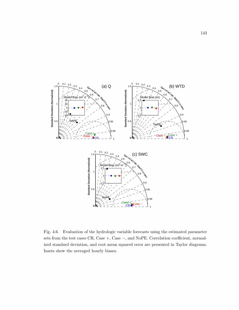
143
0
0.5
0
1
0
1.5
1
0.99
0.95
0.9
0.8
0.7
0.6
0.50.4
0.30.20.10
Sta
ndar
d D
evia
tion
(Nor
mal
ized
)
Co r r e l a t i on Coe f f i c i ent
NoPE
CR
Case +Case −
(a) Q
−40
−20
0
20
40Model Bias (m3 d−1)
0
0.5
0
1
0
1.5
1
0.99
0.95
0.9
0.8
0.7
0.6
0.50.4
0.30.20.10
Sta
ndar
d D
evia
tion
(Nor
mal
ized
)
Co r r e l a t i on Coe f f i c i ent
NoPE
CRCase +Case −
(b) WTD
−0.2
0
0.2Model Bias (m)
0
0.5
0
1
0
1.5
1
0.99
0.95
0.9
0.8
0.7
0.6
0.50.4
0.30.20.10
Sta
ndar
d D
evia
tion
(Nor
mal
ized
)
Co r r e l a t i on Coe f f i c i ent
NoPE
CRCase + Case −
(c) SWC
−0.1
0
0.1Model Bias (m3 m−3)
Fig. 4.6. Evaluation of the hydrologic variable forecasts using the estimated parameter
sets from the test cases CR, Case +, Case −, and NoPE. Correlation coefficient, normal-
ized standard deviation, and root mean squared error are presented in Taylor diagrams.
Insets show the averaged hourly biases.
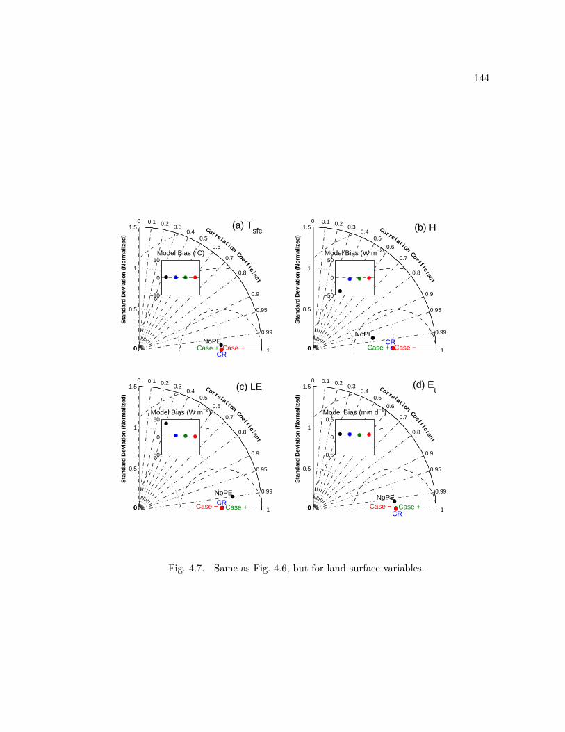
144
0
0.5
0
1
0
1.5
1
0.99
0.95
0.9
0.8
0.7
0.6
0.50.4
0.30.20.10
Sta
ndar
d D
evia
tion
(Nor
mal
ized
)
Co r r e l a t i on Coef f i c i ent
NoPE
CRCase + Case −
(a) Tsfc
−10
0
10Model Bias (°C)
0
0.5
0
1
0
1.5
1
0.99
0.95
0.9
0.8
0.7
0.6
0.50.4
0.30.20.10
Sta
ndar
d D
evia
tion
(Nor
mal
ized
)
Co r r e l a t i on Coef f i c i ent
NoPECR
Case + Case −
(b) H
−50
0
50Model Bias (W m−2)
0
0.5
0
1
0
1.5
1
0.99
0.95
0.9
0.8
0.7
0.6
0.50.4
0.30.20.10
Sta
ndar
d D
evia
tion
(Nor
mal
ized
)
Co r r e l a t i on Coef f i c i ent
NoPECR
Case +Case −
(c) LE
−50
0
50Model Bias (W m−2)
0
0.5
0
1
0
1.5
1
0.99
0.95
0.9
0.8
0.7
0.6
0.50.4
0.30.20.10
Sta
ndar
d D
evia
tion
(Nor
mal
ized
)
Co r r e l a t i on Coef f i c i ent
NoPE
CRCase +Case −
(d) Et
−0.5
0
0.5Model Bias (mm d−1)
Fig. 4.7. Same as Fig. 4.6, but for land surface variables.

145
observations available at the Shale Hills Critical Zone Observatory (SSHO) within the
Shale Hills watershed. The NoSM and NoWTD test cases eliminate soil moisture and
water table depth observations, respectively. The QST case assimilates the discharge,
soil moisture, and land surface temperature observations, which are assumed to be the
essential observations for Flux-PIHM. Fig. 4.8 presents the true values and the temporal
evolution of the parameters from those test cases. The same 30 ensemble members are
used to start each test case.
0.4
0.6
0.8
1
Θe
0
0.5
1
1.5
2
2.5
α
1
1.5
2
2.5
β
0.4
0.6
0.8
1
M A M J J
Rcmin
0
1
2
3
4
5
M A M J JMonth
S
−1
−0.5
0
0.5
1
M A M J J
lgC
zil
Control runQSSHO
NoSMNoWTDQST
Fig. 4.8. Same as Fig. 4.5, but for the test cases CR, Q, SSHO, and NoSM, NoWTD,
and QST.
The estimated values for each parameter in the different test cases are listed
in Table 4.4. The comparisons of state variables between evaluation runs using the
estimated parameter sets and the truth run are presented in Figs. 4.9 and 4.10.

146
0
0.5
0
1
0
1.5
1
0.99
0.95
0.9
0.8
0.7
0.6
0.50.4
0.30.20.10
Sta
ndar
d D
evia
tion
(Nor
mal
ized
)
Co r r e l a t i on Coe f f i c i ent
NoPE
CR
Q
SSHONoSM
NoWTDQST
(a) Q
−40
−20
0
20
40Model Bias (m3 d−1)
0
0.5
0
1
0
1.5
1
0.99
0.95
0.9
0.8
0.7
0.6
0.50.4
0.30.20.10
Sta
ndar
d D
evia
tion
(Nor
mal
ized
)
Co r r e l a t i on Coe f f i c i ent
NoPE
CR
Q
SSHONoSM NoWTD
QST
(b) WTD
−0.2
0
0.2Model Bias (m)
0
0.5
0
1
0
1.5
1
0.99
0.95
0.9
0.8
0.7
0.6
0.50.4
0.30.20.10
Sta
ndar
d D
evia
tion
(Nor
mal
ized
)
Co r r e l a t i on Coe f f i c i ent
NoPE
CR
Q
SSHONoSMNoWTD
QST
(c) SWC
−0.1
0
0.1Model Bias (m3 m−3)
Fig. 4.9. Same as Fig. 4.6, but for the test cases CR, Q, SSHO, NoSM, NoWTD, QST,
and NoPE.

147
0
0.5
0
1
0
1.5
1
0.99
0.95
0.9
0.8
0.7
0.6
0.50.4
0.30.20.10
Sta
ndar
d D
evia
tion
(Nor
mal
ized
)
Co r r e l a t i on Coef f i c i ent
NoPE
CR
Q
SSHONoSMNoWTDQST
(a) Tsfc
−10
0
10Model Bias (°C)
0
0.5
0
1
0
1.5
1
0.99
0.95
0.9
0.8
0.7
0.6
0.50.4
0.30.20.10
Sta
ndar
d D
evia
tion
(Nor
mal
ized
)
Co r r e l a t i on Coef f i c i ent
NoPE
CR
QSSHO
NoSM
NoWTDQST
(b) H
−50
0
50Model Bias (W m−2)
0
0.5
0
1
0
1.5
1
0.99
0.95
0.9
0.8
0.7
0.6
0.50.4
0.30.20.10
Sta
ndar
d D
evia
tion
(Nor
mal
ized
)
Co r r e l a t i on Coef f i c i ent
NoPE
CR
QSSHONoSM
NoWTDQST
(c) LE
−50
0
50Model Bias (W m−2)
0
0.5
0
1
0
1.5
1
0.99
0.95
0.9
0.8
0.7
0.6
0.50.4
0.30.20.10
Sta
ndar
d D
evia
tion
(Nor
mal
ized
)
Co r r e l a t i on Coef f i c i ent
NoPE
CR
QSSHO
NoSM
NoWTDQST
(d) Et
−0.5
0
0.5Model Bias (mm d−1)
Fig. 4.10. Same as Fig. 4.9, but for the land surface variables

148
Table 4.4. Estimated parameter calibration coefficients from different test cases. Es-
timated values in bold font indicate that the estimated values have errors larger than
0.5σ0.
Case Θe α β Czil Rc min S
True value 0.52 1.50 1.30 0.70 0.50 2.00
CR 0.51 1.44 1.32 0.73 0.46 2.10
Case + 0.49 1.44 1.33 0.72 0.45 2.24
Case − 0.51 1.37 1.36 0.72 0.44 1.99
Q 0.60 1.10 1.18 2.28 0.81 2.25
SSHO 0.51 1.38 1.35 0.87 0.39 2.29
NoSM 0.58 0.76 1.35 0.73 0.66 2.08
NoWTD 0.46 1.51 1.31 0.72 0.46 1.97
QST 0.47 1.52 1.30 0.68 0.56 2.55
NoPE 1.00 1.00 1.00 1.00 1.00 1.00
Fig. 4.8 and Table 4.4 show that when discharge is the only observation data set
assimilated into the system, EnKF cannot provide good estimates for model parameters
α, Czil, and Rc min, the errors of which are larger than 0.5σ0. In this test case, the hydro-
logic parameters Θe and α seem to approach to their true values, but very slowly because
only one observation is assimilated at each analysis step (Fig. 4.8). Compared with the
NoPE evaluation run, the estimated parameters from this test case strongly improve the
forecast of discharge (Fig. 4.9). Comparison of the discharge forecast with the truth
shows a high correlation coefficient (about 0.99) and comparable normalized standard
deviation with other test cases, although this test case overestimates total discharge.
The assimilation of discharge observations helps the system obtain model parameters
which could produce reasonable discharge forecast. For the other two hydrologic vari-
ables, the correlation coefficients are significantly lower than the other test cases, even
149
lower than the NoPE run. It indicates that parameters obtained in the Q case cannot
resolve the temporal variation in WTD and SWC. WTD and SWC simulations also have
large model biases, especially SWC, and the evaluation run underestimates the standard
deviation in SWC. Due to the lack of land surface variable observations, estimations of
land surface parameters are poor (Fig. 4.8 and Table 4.4). The forecast of land sur-
face variables using this parameters are worse compared with all the other test cases.
The estimated parameter by assimilating the discharge observation cannot reproduce the
temporal variation of land surface variables well (Fig. 4.10). The forecasts of Tsfc and H
also have large biases, about 7.65 ◦C for Tsfc and −36.76 W m−2 for H. The forecasts of
LE and Et, however, have relatively small biases. The mean bias in LE forecast is only
−8.17 W m−2, and the mean bias in Et forecast is −0.42 mm d−1, which is equivalent
to −12.16 W m−2 in the unit of energy.
When SWC is not assimilated into the system, EnKF cannot provide a good
estimate of α, and the errors in α is much larger than 0.5σ0 (Fig. 4.8 and Table 4.4).
The sensitivity test (Chapter 3) illustrates that the effect of α is the most significant
in SWC. In this case, EnKF underestimates α, and thus produces a large bias in SWC
(Fig. 4.9). To compensate the high bias in soil moisture, EnKF overestimates Rc min to
meet the constraints of land surface variables. As a result, although estimation of Rc min
is off, parameters α and Rc min compensate each other and produce reasonable land
surface variable forecasts, which are comparable to the control run (Fig. 4.10). But the
forecast of land surface variables is “right for the wrong reason”. Forecasts of discharge
and WTD are also comparable to the control run (Fig. 4.9). Although the bias in SWC
in this test case is much larger than in the other test cases, the correlation coefficient and

150
standard deviation of SWC forecast are comparable to the other test cases. It implies
that the parameter α is more influential in determining the mean value of SWC, rather
than the amplitude of temporal fluctuation.
Estimated parameter values from the NoWTD run are very close to the control
run (Table 4.4). The most noticeable differences of parameter evolution between those
two test cases occur in the second half of July, for parameters Θe and β (Fig. 4.8). This
is the time period when there is little precipitation, and forecasted outlet discharge rates
from all ensemble members are low. In this time period, different ensemble members
provide similar forecasts, the model discharge variance σ2m
is small, and the assimilation
of model discharge cannot make a strong impact. Because of the error in Θe in low
flow periods, the estimated Θe value is worse than in the control run (Table 4.4), and
produces a worse discharge forecast than the control run (Fig. 4.9). But for the other
hydrologic variables and land surface variables, assimilating WTD or not makes little
difference, even for the WTD forecast. It indicates that the WTD observations are only
useful in low flow periods, when WTD forecasts are better indicators of hydrologic states
than discharge forecasts.
The temporal evolution of the hydrologic parameters in the QST case is similar
with the NoWTD case (Fig. 4.8), because the hydrologic variables assimilated into those
two cases are the same. Only the parameter S has an error greater than 0.5σ0 (Table 4.4).
Hydrologic parameters are off in low flow periods because no WTD observations are
assimilated (Fig. 4.8). Although Tsfc is the only land surface observation assimilated
in this test case, the estimations of land surface parameters are very close to the true
values, except for S. The forecast of land surface variables is also comparable to the

151
control run (Fig. 4.10). The results from this test case show that Tsfc is a very good
indicator of land surface states. The results also demonstrate that Q, SWC, and Tsfc are
the essential observations for the estimation of those six model parameters at the Shale
Hills watershed.
The SSHO case does not assimilate Tsfc and Et. The estimated values of pa-
rameters, except for Rc min, are very close to true values (Table 4.4). The forecast of
hydrologic variables are almost as good as in the control run (Fig. 4.9). For the land
surface variables, the forecast of the SSHO case is only slightly worse than the control
run (Fig. 4.10). Due to the error in Rc min estimation, the SSHO case has a larger bias
in the Et forecast compared with other test cases. But the mean bias is still negligible,
only 0.22 mm d−1, equivalent to 6.37 W m−2 in the unit of energy. In spite of the lack
of Tsfc and Et observations, the assimilation of H and LE are sufficient for land surface
variable forecast. This test case shows that using the currently available observations
for parameter estimation is very promising.
There are several test cases that do not assimilate Et observations: the test cases
Q, SSHO, and QST. Results from those test cases show that as long as Tsfc or surface
heat fluxes are assimilated into the system, the system is able to obtain model parameters
that could provide reasonably good Et forecast (Fig. 4.10). Therefore, the measurement
of Et is not necessary for model calibration purpose.
It needs to be pointed out that those results are based on a perfect model, perfect
forcing data, and a perfect model domain. More observations may be needed in practical
application if the model structure is wrong.

152
4.4.4 Parameter interaction
Because EnKF is based upon ensemble generation, the relationship among dif-
ferent ensemble members reveals the interactions between model parameters. Fig. 4.11
is a scatterplot of α and β values from all ensemble members from 0000 UTC 1 July
to 0000 UTC 1 August 2009. This period includes five EnKF analysis steps. In total,
Fig. 4.11 exhibits the relationship between 150 α values and 150 β values. Parameters
α and β show high correlation during this period (Fig. 4.11), which indicates strong
interaction between them.
1 1.5 2 2.51
1.1
1.2
1.3
1.4
1.5
α
β
Fig. 4.11. Scatterplot of α and β values from all ensemble members from 0000 UTC
1 July to 0000 UTC 1 August 2009. The dashed line represents the linear fit for α-β.
The true α-β value is represented by the red dot.
153
For another example, Fig. 4.12 shows the scatterplot of Rc min and β values from
all ensemble members from 0000 UTC 1 April to 0000 UTC 1 May 2009. This period
includes eight EnKF analysis steps. In total, Fig. 4.12 shows the relationship between
240 Rc min values and β values. Except for one ensemble member with high β values,
Rc min and β from the other ensemble members show relatively high correlation during
this period (Fig. 4.12). The true Rc min-β value is also very close to the fitted line. At
the watershed scale, higher β values lead to lower soil water content (Fig. 3.8), which
limits the transpiration. To compensate for β, EnKF decreases Rc min for those ensemble
members with higher β values, and increases Rc min for those ensemble members with
lower β values. This parameter interaction between the hydrologic parameter and the
land surface parameter also reveals land surface-subsurface interaction.
4.5 Discussions and conclusions
Because of their high computational demands, high dimensional variable and pa-
rameter space, strong nonlinearity, and strong parameter interaction, it is extremely
difficult to perform parameter estimation for physically-based hydrologic models. This
chapter presents the first parameter estimation using EnKF for a physically-based land
surface hydrologic model. Synthetic experiments are performed to find the optimal time
interval for data assimilation, to test the capability of EnKF, and to examine the effects
of assimilating different observations.
The test cases with different assimilation intervals show that the sponge effect
degrades the estimation of hydrologic parameters. In the dry periods, the appropriate
assimilation interval should be similar to the relaxation time of the watershed to eliminate

154
0.4 0.5 0.61.1
1.2
1.3
1.4
1.5
1.6
1.7
Rcmin
β
Fig. 4.12. Same as Fig. 4.11, but for Rc min and β values from 0000 UTC 1 April to
0000 UTC 1 May 2009.

155
the impacts of the sponge effect. In the wet periods, the assimilation interval could be
shorter than the relaxation time. In this study, assimilation intervals of 72 hours in
wet periods and 144 hours in dry periods are sufficient. Results show that with the
assimilation of appropriate observations and appropriate assimilation intervals, EnKF is
able to provide good estimations of parameter values for Flux-PIHM. The different initial
ensemble means have little effects on EnKF estimation, which indicates high reliability
of EnKF. Results demonstrate that, given a limited number of site-specific observations,
an automatic sequential calibration method (EnKF) can be used to optimize Flux-PIHM
for watersheds like Shale Hills.
Assimilating discharge alone can improve the forecast of discharge, but the im-
provement in the discharge forecast is limited compared with other test cases. The
forecast of subsurface variables (SWC and WTD) and land surface variables in this test
case is poor. The forecast of discharge would be significantly improved if WTD or SWC
observations were assimilated. Those findings agree with the findings of Camporese et al.
(2009) and Lee et al. (2011). This test case (Q) shows that although land surface and
hydrologic components have considerable interaction, assimilating discharge observation
alone cannot provide reliable land surface parameter estimation.
The effect of WTD observations are not strong when SWC observations are as-
similated, except for low flow periods. In low flow periods, different ensemble members
produce similar discharge observations and the discharge observations are not effective
indicators of watershed hydrologic states. This is when WTD observations are the most
helpful. SWC observations are necessary for the accurate estimates of the parameter α.
When SWC is not assimilated, the forecasts of land surface variables are still comparable

156
to other test cases. However, EnKF produces errors in other parameters, especially land
surface parameters, to compensate the errors in α.
Both Tsfc and surface heat fluxes are good indicators of land surface states. As-
similation of either Tsfc or surface heat fluxes are sufficient for land surface parameter
estimation. Observations of Et are not necessary for model calibrations. The SSHO test
case assimilates observations which are currently available at the Shale Hills watershed.
The results are very encouraging. Except for Rc min, estimated values of all model pa-
rameters are very close to their true values. The forecasts of hydrologic variables and
land surface variables are also comparable to the control run. It indicates that using
the currently available observation data sets for EnKF parameter estimation is very
promising.

157
Chapter 5
Flux-PIHM Parameter Estimation
Using Ensemble Kalman Filter:
A Real-Data Experiment
5.1 Introduction
The uncertainties in model parameters have been the main source of uncertainties
for physically-based hydrologic models (Moradkhani and Sorooshian 2008). The recently
proposed ensemble Kalman filter (EnKF; Evensen 1994) provides a promising approach
for spatially-distributed physically-based hydrologic model auto calibration. In Chap-
ter 4, multiple-parameter estimation for a physically-based land surface hydrologic model
using EnKF is tested. The modeling and data assimilation system is implemented at the
Shale Hills watershed in central Pennsylvania, where the Shale Hills Critical Zone Obser-
vatory (SSHO) is located. Synthetic experiments are performed to test the capability of
EnKF in parameter estimation for the land surface hydrologic model Flux-PIHM. Opti-
mal assimilation intervals and effects of different observations have been studied. Results
from the synthetic data experiments illustrate that EnKF is capable of providing good
estimations for multiple Flux-PIHM model parameters. In a specific test case, synthetic
observations of currently available observations at SSHO are assimilated to test the best
scenario for the real-data experiments, and the results are very encouraging. Estimations
of five out of the six parameters are very close to the true values, and the forecasts of
hydrologic and land surface variables compare well with the truth run.

158
Real-data experiments, however, have extra difficulties compared with the syn-
thetic data experiments. In the synthetic experiments, the only uncertainty exist are the
parameter uncertainty and the uncertainty in assimilated observations. Forecast mod-
els have perfect forcing data, perfect static input data, and perfect model structures.
Thus, all “observed” states in synthetic experiments are “achievable”. When real data
are used, however, model errors consist of errors from forcing data, domain configu-
ration, and model structure. Some observed states in real-data experiments might be
“unachievable” with plausible parameter values due to those errors.
Consider the forcing data error for example. Assume a rain gauge or data logger
malfunctions during a heavy rainfall event, and misses the precipitation event. Using
this recorded precipitation rate as the atmospheric forcing, the model certainly could
not reproduce the observed discharge peak, i.e., the observed state is unachievable with
plausible parameter values. If the observed discharge peak for this event is assimilated,
the model error would be huge. If the forcing data errors are not explicitly taken into
account, EnKF would attribute all model errors to parameter errors. As a result, param-
eter values might be driven to an unreasonable value to mitigate the huge model error.
The biased parameters would affect the performance of the following forecasts. Consider
a model structural error, for example, a model that does not have macropore processes.
When the soil is relatively dry and the macropores are not working, EnKF should be
able to provide good estimations of the soil matrix conductivities. When the soil is ex-
tremely wet, and the macropores are playing a role, EnKF would increase the soil matrix
conductivities to simulate the macropore effects. The estimations would be far off their
optimal values. The temporal variation of the soil matrix conductivities might jump

159
between two totally different states because EnKF tries to compensate the model struc-
tural error by adjusting model parameter values. The other input data, e.g., topography
data, soil map, vegetation map, domain decomposition, may also cause persistent bias in
the model forecast. Those errors in forcing data, in model structure, and in other input
data pose extra difficulties for finding the optimal parameter values. Data assimilation
must be performed with extreme care because the large change in parameter values and
parameter uncertainties may lead to filter divergence (Anderson and Anderson 1999).
Although the synthetic data experiments yield encouraging results, the capabil-
ity of an EnKF system to optimize Flux-PIHM using real observations still needs to
be demonstrated. Extensive field surveys have been conducted and abundant high-
temporal-resolution meteorological data, surface flux data, and hydrological data have
been collected at SSHO. The broad array of observations at SSHO provides an opportu-
nity for real-data experiment of Flux-PIHM parameter estimation using EnKF. In this
chapter, real-data experiment of Flux-PIHM model parameter estimation using EnKF
is performed. As results in Chapter 4 provide helpful guidance for the set-up of real-
data experiments, this chapter follows the framework provided in the previous chapter.
The ability of EnKF to estimate parameters in Flux-PIHM with the assimilation of field
observations is tested. Model performances with the estimated parameter values and
manually calibrated values are compared to assess the quality of estimated parameter
values.

160
5.2 Preprocessing of observations
The Flux-PIHM EnKF data assimilation system developed in Chapter 4 is imple-
mented at the Shale Hills watershed. The real observations assimilated into the system
are:
(1) Outlet discharge rate (Q);
(2) Water table depth at RTHnet wells (WTD);
(3) Integrated soil moisture content over soil column RTHnet wells (SWC);
(4) Spatial average sensible heat flux (H) via above-canopy eddy covariance measure-
ments; and
(5) Spatial average latent heat flux (LE) via above-canopy eddy covariance measure-
ments.
Details of the above observations can be found in Section 2.3.3.
To avoid unachievable observed states causing dramatic changes in parameter
values, the assimilated observations are preprocessed: the uncertainties of observations
are specified, and some observations are eliminated. The principles for the preprocessing
are to assign relatively large uncertainty to observations to moderately reduce the impact
of observations, and to eliminate those states that cannot be achieved by the model.
Discharge is measured with a stream gauge at the outlet of catchment. A V-
notch weir measures water level, which is then converted to discharge using a rating
curve developed by Nutter (1964) for the V-notch weir at the Shale Hills watershed.

161
The calibrated rating curve is:
Q =
2446.58 × 10−5.56+181.67−2778.15x2
, 0 < x ≤ 0.034 m,
3.08 × 10⁴ × x2.46, 0.034 m < x < 0.100 m
3.12 × 10⁶ × x4.47, x > 0.100 m
(5.1)
where x is measured water level (m), and Q is discharge rate (m3 d−1). Same as in
Chapter 4, discharge observations are converted to log space prior to analysis steps.
Fig. 5.1 shows the rating curve in log space. Assuming the representative observation
error for water level is 1 mm, the green and red lines show the rating curves for x+0.001 m
(Qx+0.001) and x − 0.001 m (Qx−0.001), respectively.
0 0.05 0.1 0.15 0.2 0.25 0.3−6
−4
−2
0
2
4
6
8
10
x (m)
ln Q
[ln(
m3 d
−1)]
x+0.001Q
x−0.001
Fig. 5.1. Rating curve for SSHO V-notch weir (blue line). The green and red lines
represent rating curves with 1 mm error in measured water level.

162
It is clear that the errors of Qx−0.001 and Qx+0.001 are larger at low discharge rates
in log space. It means that the same observation error in river level would produce a
much larger discharge error in log space when discharge rate is low than when discharge
rate is high. The blue curve in Fig. 5.2 represents the average error for Qx−0.001 and
Qx+0.001, calculated as 0.5 (|ln Qx+0.001 − ln Q| + |ln Qx−0.001 − lnQ|). The dashed black
curve in Fig. 5.2 is the manual fit for the average error. The fits have three linear
segments, corresponding to the three cases in Eq. (5.2):
σQ =
−0.1 ln(Q + ǫ) + 0.4, ln(Q + ǫ) ≤ 1.97 ln(m3 d−1),
−0.056 ln(Q + ǫ) + 0.309, 1.97 ln(m3 d−1) < ln(Q + ǫ) < 4.63 ln(m3 d−1),
0.05, ln(Q + ǫ) ≥ 4.63 ln(m3 d−1).
(5.2)
where σQ represents the observation error of discharge in log space, and ǫ is a very small
number to avoid taking logarithm of a zero discharge.
Converting discharge to log space improves EnKF performance (Clark et al. 2008),
but also exaggerates forecast errors for low flows. For example, when the forecast is
0.1 m3 d−1 and the observation is 0.01 m3 d−1, the forecast error is the same in log space
as when the forecast is 100 m3 d−1 and the observation is 1000 m3 d−1. To avoid the
exaggerated large errors at low flows, a 1 m3 d−1 discharge rate is added to both the
observation and the forecasts, after calculating the observation errors using the observed
discharge rate with Eq. (5.2).
Observations of WTD and SWC are calculated by averaging multiple groundwater
level measurements and volumetric soil moisture content measurements at the RTHnet

163
−4 −2 0 2 4 6 80
0.2
0.4
0.6
0.8
1
ln Q [ln(m 3 d−1)]
ln Q
Err
or [l
n(m
3 d−1
)]
Fig. 5.2. Average error for rating curves with 1 mm error in measured water level. The
black dashed line represents the manual fit of the average error.
wells. The standard deviations between different wells and soil moisture sensors are
specified as observation errors σWTD and σSWC.
In Flux-PIHM and almost all LSMs, the surface energy balance is closed, i.e.,
Rn −G = H + LE, where Rn is the net radiation, and G is the ground heat flux. Eddy
covariance measurements, however, always fail to close the energy budget, and H + LE
tend to be less than Rn−G (McNeil and Shuttleworth 1975; Fritschen et al. 1992; Twine
et al. 2000). The surface heat fluxes measured at SSHO using eddy-covariance method
(H and LE) may have consistent low bias. Thus, the mid-day (1700 UTC) surface heat
fluxes are rescaled using net radiation measurements at SSHO. As a highly-forested site,
ground heat fluxes at the Shale Hills watershed are small. At the Shale Hills watershed,
in growing seasons, simulated mid-day (1700 UTC) ground heat fluxes are always below
164
3% of Rn, and the average ratio between simulated ground heat flux and net radiation
in 2009 is about 4%. We therefore treat G as negligible, and rescale H + LE using Rn.
When the sum of gap-filled hourly averaged surface heat fluxes H0 + LE0 < Rn, the
surface heat fluxes are rescaled as
H =H0
H0 + LE0
Rn, (5.3a)
and
LE =LE0
H0 + LE0
Rn. (5.3b)
This rescaling does close the surface energy balance on average, but does not eliminate
the random variability in H and LE that occurs with half-hourly flux measurements
(e.g., Berger et al. 2001; Richardson et al. 2006). In addition, the radiation forcing
(downward solar radiation and downward longwave radiation) data used for Flux-PIHM
are not collected SSHO, but at the surface radiation budget network (SURFRAD) Penn
State University station, which is 6.48 km away from the Shale Hills watershed. Both
the random errors in measured surface heat fluxes, and the different radiation conditions
at SURFRAD station and SSHO could produce unachievable states for Flux-PIHM.
To avoid those states, the rescaled mid-day heat fluxes are compared with manually
calibrated Flux-PIHM surface heat flux predictions. If the model error is too large,
those rescaled heat fluxes are eliminated. The random observation errors σH and σLE
are assumed to be 20% of observations, 0.2H and 0.2LE.

165
5.3 Experimental setup
The Flux-PIHM EnKF data assimilation system developed in Chapter 4 is adopted
in this study. The grid configuration, vegetation map, soil map, atmospheric forcing, and
a priori input data are the same as in Chapter 2. The parameters to be estimated are
the same as in Chapter 4:
(1) Effective porosity Θe;
(2) van Genuchten soil parameter α (van Genuchten 1980);
(3) van Genuchten soil parameter β (van Genuchten 1980);
(4) Zilitinkevich parameter (Zilitinkevich 1995) Czil;
(5) Minimum stomatal resistance Rc min; and
(6) Reference canopy water capacity S [Eq. (2.15)].
A total of 30 ensemble members are used for the experiment. Those 30 ensemble members
are the same as in the control run in Chapter 4. The ensemble members are generated
by randomly perturbing the calibration coefficients of those six parameters within their
plausible ranges. The parameters that are not estimated are set to their manually cali-
brated values as in Table 2.6. For each parameter (calibration coefficient) φ, the values
are randomly drawn from a Gaussian distribution, with an initial standard deviation of
σ0 = 0.2 (φmax − φmin). Among those parameters, Czil is perturbed in log space. The
correlation coefficients between different parameters are lower than 0.25, to ensure each
parameter varies independently. In Chapter 4, the optimal assimilation interval for the

166
synthetic experiment is found to be around three days in wet periods, and about six
days in dry periods. In real-data experiments, however, the fluctuations of parameter
values might be stronger than in the synthetic data experiments to compensate errors
from other sources. Stronger fluctuation of parameter may intensify the sponge effect
and require an even longer adjustment period. To safely eliminate any impact from the
sponge effect, the assimilation interval is set to 168 hours (seven days), which is about
the relaxation time for the Shale Hills watershed, regardless of wet or dry periods. All
ensemble members start from 0000 UTC 10 March, from saturation in the relaxation
mode. The first set of observations is assimilated at 1700 UTC 4 April 2009. The sim-
ulation period prior to 1700 UTC 4 April is used for spin-up. The calibration period is
from 4 April to 1 September 2009. The time for assimilating the first set of observations
is chosen for two reasons. First, the eddy covariance surface heat fluxes are only available
after 1 April 2009. Second, the time is chosen to include the discharge peak on 20 June
2009 considering the assimilation interval. Among the six model parameters, Θe has the
strongest impact on peak discharge rate, and its influence is not significant in low flow
periods. In other words, for the accurate forecast of a discharge peak, an accurate Θe
value is needed, while the calibration of Θe requires the assimilation of peak discharge
observations. Therefore, the highest discharge peak during the calibration period has to
be assimilated to make the best use of available observations.
In order to avoid driving the model into unrealistic states, the uncertainties in
observations must be carefully weighted according to their relative impacts on model
parameters. The observation errors when assimilated into the system should at least
be comparable to the uncertainty of the ensemble forecast, if not smaller than, to make

167
impacts on variable and parameter estimation. In order to do this, the observation
errors when assimilated into the system could be different from the assumed or real
observation errors. The synthetic experiments in Chapter 4 provide helpful guidance for
specifying the observation errors. But the weights of the observations need to be relaxed
appropriately as compared to the synthetic experiments, to avoid fatal impacts from
unachievable states. The errors in the observations when assimilated into the system in
the real-data experiment are presented in Table 5.1.
Table 5.1. Errors in the observations when assimilated into the system in the real-data
experiment. The σ values represent the assumed or real observation uncertainties.
Q WTD SWC H LE
2σQ σWTD 0.25σSWC 0.5σH 0.5σLE
5.4 Results
Fig. 5.3 presents the temporal evolution of the calibration coefficients of the es-
timated parameters. The shaded area around the estimated value represents the one
standard deviation (1-σ) spread of the ensemble spread. The manually calibrated pa-
rameter values are also presented for reference purpose.
Among those six parameter, the standard deviations (σ) of α, β, and Rc min
decrease to 0.25σ0, i.e., those parameters converged. But the standard deviation of
Rc min decreases to under 0.25σ0 because the estimated parameter values are very close
to the boundary, and the quality control process has to decrease the ensemble spread to

168
Θe
0.4
0.6
0.8
1
α
0
0.5
1
1.5
2
2.5
β
1
1.5
2
2.5
A M J J A
Rcmin
0.4
0.6
0.8
1
A M J J AMonth
S
0
1
2
3
4
5
A M J J A
lgCzil
−1
−0.5
0
0.5
1
Fig. 5.3. Temporal evolution of estimated parameters (blue lines) in real-data exper-
iment. The dashed lines represent the manually calibrated parameter values, and the
shaded areas represent the 1-σ spread.
make sure all ensemble members are within the predefined range. For parameters that
converge during the calibration period, i.e., α, β, and Rc min, the temporal averages of
ensemble mean values after convergence are calculated as estimated parameter values.
For the other parameters which do not converge, the temporal averages of ensemble
mean values between 1 August and 1 September are calculated as estimated parameter
values. The parameter values estimated by EnKF and manual calibration are presented
in Table 5.2.
Except for parameter S, parameter values estimated by EnKF are very close
to the manually calibrated values (Table 5.2), especially for parameters α, β, and Czil.
Parameter Θe has two dramatic changes in parameter value during the calibration period
(Fig. 5.3). During the first analysis steps, the estimation of Θe is approaching the

169
Table 5.2. Estimated parameter calibration coefficients from the real-data experiment.
The manual calibrated values are presented for reference purpose. The differences be-
tween the manual calibrated values and the EnKF estimated values are also presented.
Here R = φmax − φmin represents the plausible range for each calibration coefficient.
Case Θe α β Czil Rc min S
EnKF 0.60 1.55 1.33 0.81 0.36 3.80
Manual calibration 0.52 1.50 1.30 0.70 0.50 2.00
Difference 0.09R 0.02R 0.02R 0.03R 0.16R 0.36R
manually-calibrated value. But a dramatic change of Θe appears on 2 May, and the
parameter value deviates from the manually-calibrated value. In the manual calibration
process, from the end of April to the beginning of May, Flux-PIHM fails to reproduce
the temporal variation of low flows (Fig. 2.8). This model error might be caused not
only by parameter values, but also errors in model structures and static input data. It
is possible that, because structural errors and static input data errors are be addressed
by the current version of EnKF, all model errors are attributed to parameter errors, and
the Θe value is changed dramatically by EnKF to compensate the large model error.
The following discharge observations assimilated are low flows, which make little impact
on Θe. The parameter Θe is not driven to its optimal value until the discharge peak on
20 June is assimilated. After the discharge peak is assimilated, EnKF adjusts Θe value
dramatically towards the manually calibrated value, and the parameter value generally
stabilizes afterwards. For all parameters, the fluctuations of parameter values have
larger amplitudes than in the synthetic data experiments (Figs. 4.5 and 5.3), because
parameter values are adjusted to compensate model errors, forcing data errors, etc. It
is also possible that those parameters are time dependent.
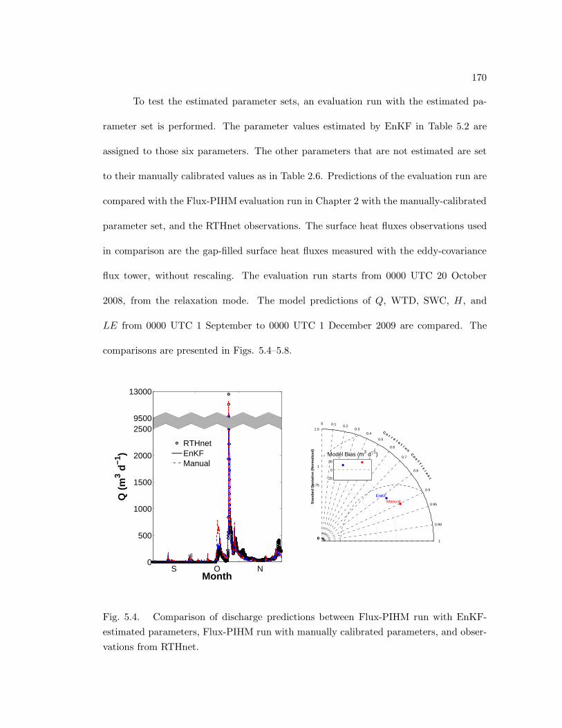
170
To test the estimated parameter sets, an evaluation run with the estimated pa-
rameter set is performed. The parameter values estimated by EnKF in Table 5.2 are
assigned to those six parameters. The other parameters that are not estimated are set
to their manually calibrated values as in Table 2.6. Predictions of the evaluation run are
compared with the Flux-PIHM evaluation run in Chapter 2 with the manually-calibrated
parameter set, and the RTHnet observations. The surface heat fluxes observations used
in comparison are the gap-filled surface heat fluxes measured with the eddy-covariance
flux tower, without rescaling. The evaluation run starts from 0000 UTC 20 October
2008, from the relaxation mode. The model predictions of Q, WTD, SWC, H, and
LE from 0000 UTC 1 September to 0000 UTC 1 December 2009 are compared. The
comparisons are presented in Figs. 5.4–5.8.
0
0.75
0
1
0
1.5
1
0.99
0.95
0.9
0.8
0.7
0.6
0.5
0.40.3
0.20.10
Sta
ndar
d D
evia
tion
(Nor
mal
ized
)
C o r r e l a t i o n C
oe
ff
i ci e
nt
EnKFManual
−20
0
20
Model Bias (m3 d−1)
Month
Q (
m3 d
−1)
S O N 0
500
1000
1500
2000
25009500
13000
RTHnetEnKFManual
Fig. 5.4. Comparison of discharge predictions between Flux-PIHM run with EnKF-
estimated parameters, Flux-PIHM run with manually calibrated parameters, and obser-
vations from RTHnet.

171
0
0.75
0
1
0
1.5
1
0.99
0.95
0.9
0.8
0.7
0.6
0.5
0.40.3
0.20.10
Sta
ndar
d D
evia
tion
(Nor
mal
ized
)
C o r r e l a t i o n C
oe
ff
i ci e
nt
EnKF
Manual
−0.4
−0.2
0
0.2
Model Bias (m)
0
0.2
0.4
0.6
0.8
1
1.2
1.4
1.6
1.8
2
S O NMonth
WT
D (
m)
EnKFManualRTHnet
Fig. 5.5. Same as Fig. 5.4, but for WTD.
Performance of the Flux-PIHM evaluation run with the EnKF-estimated parame-
ter set is comparable to the Flux-PIHM run with the manually-calibrated parameter set
(Figs. 5.4–5.8). For discharge prediction, the manually-calibrated parameters provide
better prediction for the highest discharge peak event, but EnKF-estimated parameters
perform relatively better for other time periods (Fig. 5.4). Although the manual calibra-
tion run has better correlation with observation, it has a larger standard deviation and
mean bias compared with EnKF-estimated parameters. For WTD and SWC, EnKF-
estimated parameters perform slightly better than the manually-calibrated parameters
(Figs. 5.5 and 5.6). Both Flux-PIHM evaluation runs yield higher surface heat fluxes, but
this is expected given the rescaling of H and LE observation data (Figs. 5.7 and 5.8).

172
0
0.75
0
1
0
1.5
1
0.99
0.95
0.9
0.8
0.7
0.6
0.5
0.40.3
0.20.10
Sta
ndar
d D
evia
tion
(Nor
mal
ized
)
C o r r e l a t i o n C
oe
ff
i ci e
nt
EnKFManual
−0.05
0
0.05Model Bias (m3 m−3)
0.1
0.15
0.2
0.25
0.3
0.35
0.4
S O NMonth
SW
C (
m3 m
−3)
EnKFManualRTHnet
Fig. 5.6. Same as Fig. 5.4, but for SWC.
0
0.75
0
1
0
1.5
1
0.99
0.95
0.9
0.8
0.7
0.6
0.5
0.40.3
0.20.10
Sta
ndar
d D
evia
tion
(Nor
mal
ized
)
C o r r e l a t i o n C
oe
ff
i ci e
nt
EnKF Manual
−20
0
20Model Bias (W m−2)
0 6 12 18 24−50
0
50
100
150
200
250
Time (UTC)
H (
W m
−2)
EnKFManualRTHnet
Fig. 5.7. Same as Fig. 5.4, but for H, and plotted as averaged daily cycles.

173
0
0.75
0
1
0
1.5
1
0.99
0.95
0.9
0.8
0.7
0.6
0.5
0.40.3
0.20.10
Sta
ndar
d D
evia
tion
(Nor
mal
ized
)
C o r r e l a t i o n C
oe
ff
i ci e
nt
EnKFManual
−20
0
20Model Bias (W m−2)
0 6 12 18 24−50
0
50
100
150
200
250
Time (UTC)
LE
(W
m−2
)
EnKFManualRTHnet
Fig. 5.8. Same as Fig. 5.4, but for LE, and plotted as averaged daily cycles.
Compared with the manually-calibrated parameters, the EnKF-estimated parameters
have smaller bias in H, but larger bias in LE.
When estimating those six parameters using EnKF, other parameters are fixed at
their manually calibrated values. Therefore, the impacts of the other parameters cannot
be addressed. It is possible that if more parameters are estimated using EnKF, the
optimized parameter set might perform better.
5.5 Discussions and conclusions
Chapter 4 provides the framework for automatic Flux-PIHM parameter estima-
tion, and shows encouraging results using synthetic observations. The effectiveness of
parameter estimation using EnKF for Flux-PIHM using real data is tested in this chap-
ter.

174
Results show that for five out of the six parameters, parameter values estimated
by EnKF are very close to their manually calibrated values. The fluctuations of parame-
ter values are much stronger than in the synthetic experiment, the reason might be that
parameter values are adjusted to compensate the errors from other sources. The tempo-
ral revolution of Θe illustrates that the performance of parameter estimation might be
affected by model structural errors and other errors. Forecasts using EnKF-estimated
parameters and manually calibrated parameters are not much different. Manually cal-
ibrated parameters provide better discharge forecast for the highest discharge peak in
October, but EnKF-estimated parameters provide better forecasts for WTD and SWC.
Forecasts of surface heat fluxes are also similar. Compared with the manual calibration,
EnKF-estimated parameters provide similar forecasts, but the calibration process is au-
tomatic, much less time-consuming, and much less labor-intensive. Although automatic
parameter estimation is more affected by model structure errors, forcing data errors,
and observation errors, it could provide good estimation of parameter values given ap-
propriate treatment of observation uncertainties, assimilation intervals, and length of
observation records.
The observation uncertainties need to be adjusted to provide reasonable obser-
vation weights. Compared with synthetic experiments, observation weights should be
smaller (observation uncertainties should be larger) to avoid impacts of unachievable
states. The principle is that the observation errors when assimilated into the system
should at least be comparable to the uncertainty of the ensemble forecast, if not smaller
than, to make impacts on variable and parameter estimation. The observation errors
when assimilated into the system could be different from the assumed or real observation

175
errors. Although the calibration of parameters using EnKF is automatic, the “calibra-
tion” of observation uncertainties is manually performed. It is true that it may take
several test runs to find the appropriate observation uncertainties, but it is still much
more efficient than manual calibration of model parameters. The adjustment of obser-
vation uncertainties could also help reflect the importance of different observations. For
example, if the forecasting of discharge is of particular interest, the observation uncer-
tainty for discharge could be moderately reduced when assimilated into the system, to
add extra weight to the discharge observations.
The current version of EnKF in this study does not take into account forcing error
and model structural errors. Perturbing the atmospheric forcing by adding random
errors to the forcing data, or add atmospheric forcing variables to the joint variable-
parameter vector could help address the forcing errors. Perturbing more parameters
without estimating them might help include the model structural errors.
This study illustrates the effectiveness of automatic parameter estimation for a
physically-based land surface hydrologic model using EnKF at a small-scale watershed.
With the rapid evolution of computer power and parallel computing techniques, more
ensemble runs with higher dimension model grids could be accomplished. The prospect
of calibrating multiple model parameters for physically-based land surface hydrologic
model on large watersheds is promising. With extra care of parameter fluctuation, the
current data assimilation system could also be used for real-time hydrologic and land
surface forecast.

176
Chapter 6
Summary
There has been recent interest in incorporating hydrologic components into the
land surface models (LSMs). The significance is two-fold. For LSMs, the incorporated
hydrologic component improves runoff prediction and soil moisture prediction. Those
improvements would help the model provide better surface heat flux predictions, and
also more accurately represent the memories of atmospheric anomalies. For hydrologic
models, the improved evapotranspiration simulation could result in better flood/drought
forecasting.
In this study, a coupled land surface hydrologic model is developed and tested at
a small watershed in central Pennsylvania. To evaluate the model predictions, the model
is calibrated manually using the trial and error method, and the model predictions are
compared with observations. Multiple observations are used in the calibration and eval-
uation processes. This calibration process is highly time-consuming and labor-intensive.
To reduce the workload for model calibration, an automatic calibration method using
the data assimilation method is developed. Both synthetic data experiments and real
data experiments are performed to test the effectiveness of the data assimilation system.

177
6.1 Coupled land surface hydrologic model
A coupled land surface hydrologic model, Flux-PIHM is developed in this study.
The model couples the Penn State Integrated Hydrologic model (PIHM; Qu 2004; Qu
and Duffy 2007; Kumar 2009) with a land surface scheme adapted from the Noah LSM
(Chen and Dudhia 2001; Ek et al. 2003). The hydrologic component and the land
surface component are closely coupled by exchanging water table depth, infiltration rate,
recharge rate, soil water storage, evapotranspiration rate, and net precipitation between
each other. The model is implemented at the Shale Hills watershed (0.08 km2) in central
Pennsylvania, where the Shale Hills Critical Zone Observatory (SSHO) resides.
Flux-PIHM is comprehensively calibrated with in situ discharge, water table
depth, soil water content, soil temperature, sensible heat flux, and latent heat flux mea-
surements collected at SSHO in June and July 2009. Model performance of Flux-PIHM
for year 2009 is evaluated. Generally, Flux-PIHM predictions of discharge, water table
depth, soil moisture, soil temperature, and surface heat fluxes compare well with the
measurements. The performance of Flux-PIHM discharge forecasting in the Shale Hills
watershed is comparable to a state-of-the-art conceptual model in similar watersheds.
Performances of Flux-PIHM are compared with PIHM Version 2.0 (PIHM V2). Results
indicate that by incorporating a surface energy balance scheme into the model, Flux-
PIHM slightly outperforms PIHM V2 in hydrologic predictions as well as evapotranspi-
ration predictions. For a specific peak discharge event, those two models, which have the
same hydrologic scheme but different land surface schemes, provide significantly different

178
forecasts of discharge rate and timing, which shows the impact of evapotranspiration on
discharge forecasting.
Flux-PIHM adds surface energy balance simulation to PIHM and improves the
predictions of both discharge and evapotranspiration. Because of its ability of accurately
simulating land surface and subsurface variables, the model is an ideal tool for the study
of land surface subsurface interaction. It is expected that such coupled models could
yield improvements in long-term weather forecasting, short-term climate forecasting,
and flood drought forecasting.
For the model test at the Shale Hills watershed, Flux-PIHM is calibrated man-
ually. As a physically-based land surface hydrologic model, the number of parameters
and the intensity of interactions among model parameters make the manual calibration
process extremely difficult. The calibration process is the most challenging step when im-
plementing Flux-PIHM at the Shale Hills watershed. The difficulty of calibration could
pose obstacles for future applications of such models onto different watersheds. An
automatic calibration technique is therefore required for the calibration of Flux-PIHM.
6.2 Flux-PIHM parameter estimation using the ensemble Kalman fil-
ter
The recently proposed ensemble Kalman filter (EnKF; Evensen 1994) provides a
promising approach for the automatic calibration of physically-based models like Flux-
PIHM. This study presents the first attempt of physically-based land surface hydrologic
model parameter estimation using EnKF. By incorporating EnKF, the Flux-PIHM data

179
assimilation system is able to perform simultaneous state and parameter estimation us-
ing state augmentation technique. The covariance relaxation method, the conditional
covariance inflation method, and a quality control process are used to avoid filter di-
vergence and to constrain the state variables and model parameters in their physically
plausible ranges. The land surface hydrologic modeling and data assimilation system is
implemented at the Shale Hills watershed.
Synthetic experiments are first performed to test the framework. Six Flux-PIHM
parameters, including three hydrologic parameters and three land surface parameters
are chosen for estimation. Those parameters are selected from a Flux-PIHM parameter
sensitivity test, which examines the parameter identifiability. The parameters chosen in
this study have relatively high distinguishability, observability, and simplicity. Synthetic
observations of discharge, water table depth, soil water content, surface skin temperature,
sensible heat flux, latent heat flux, and transpiration rate are extracted from a truth run.
The synthetic experiments provide the framework for Flux-PIHM parameter es-
timation using EnKF. Results show that with appropriate observations, observation
uncertainties, and assimilation intervals, EnKF is able to provide good estimations of
parameter values for Flux-PIHM. The influences of initial guesses are negligible. The
minimum assimilation interval for dry period is found to be about six days, which is
similar to the relaxation time of the watershed. The assimilation interval for wet period
is found to be about three days. Assimilation intervals shorter than the minimum would
suffer from the sponge effect which degrades parameter estimation performance. Obser-
vations of discharge, soil moisture, and surface temperature (or surface heat fluxes) are
found to be critical for the accurate estimation of those six parameters.

180
A real-data experiment is performed to further test the effectiveness of EnKF
in Flux-PIHM parameter estimation. The SSHO in situ measurements of discharge,
water table depth, soil moisture, sensible heat flux, and latent heat flux are preprocessed
and assimilated into the system for parameter estimation. The uncertainties of different
observations are adjusted to provide reasonable weights for observations. The principle
of adjustment is that the observation errors when assimilated into the system should
at least be comparable to the uncertainty of the ensemble forecast, if not smaller than,
to make impacts on variable and parameter estimation. The observation errors when
assimilated into the system could be different from the assumed or real observation
errors.
Although model structure errors, forcing errors, and static input data errors pose
extra difficulties for real-data experiments, EnKF is able to provide reliable estimation
of model parameters. For five out of the six parameters, parameter values estimated
by EnKF are close to their manually calibrated values. The fluctuations of parameter
values are much stronger than in the synthetic experiments, the possible reason is that the
parameters are adjusted to compensate the errors from other sources. The Flux-PIHM
predictions using EnKF-estimated parameters and manually-calibrated parameters are
similar.
EnKF is capable of performing automatic parameter estimation for Flux-PIHM,
a complex, physically-based land surface hydrologic model. EnKF also gives estimations
of parameter uncertainties and forecast uncertainties. The data assimilation system
makes it possible to perform uncertainty forecasting using a deterministic model. The

181
automatic parameter estimation would save lots of work and time for the implemen-
tation of physically-based models onto different watersheds. Because of the advantage
of sequential calibration method, this modeling and data assimilation system can be
used for real-time land surface and hydrologic forecasting. The data assimilation system
could also be helpful for the observational system design, by testing the influences of
assimilated observations on model forecasts.
6.3 Land surface subsurface interaction
One of the goals for this study is to explore the interaction between land surface
and subsurface. The developed land surface hydrologic model provides good predictions
of both land surface and subsurface, and is therefore a reliable tool for the exploration
of land surface subsurface interaction.
Flux-PIHM simulations for 2009 show that surface heat fluxes exhibit correlations
with the change of water table depth. The coupling between the land surface and the
subsurface is especially strong near the river, where the water table depth has direct
impact on surface heat fluxes. The annual average sensible and latent heat fluxes in
different grids are mainly affected by the vegetation types.
In the Flux-PIHM parameter sensitivity test, it is found that hydrologic param-
eters have significant influences on land surface variables, while land surface parameters
also have considerable impact on hydrologic variables. Soil moisture acts as a link be-
tween the land surface and the subsurface. The hydrologic component affects the soil
water content by infiltration, groundwater recharge, and change of groundwater level;
and the change of soil moisture could then affect the partitioning of available energy into

182
sensible and latent heat fluxes, affect soil heat capacity, and affect thermal conductivity.
The land surface component influences the soil water content by extracting water from
subsurface via evapotranspiration, and the change of soil moisture could then influence
the partitioning of incoming precipitation into infiltration and surface runoff, influence
hydraulic conductivity, and influence groundwater recharge. Because of the strong inter-
action between the land surface and the hydrologic components, it is almost impossible
to calibrate the hydrologic component without affecting land surface forecasting, or to
calibrate the land surface component without affecting hydrologic forecasting. The land
surface and subsurface must be treated as an integral.
Comparisons between Flux-PIHM and PIHM V2 show that evapotranspiration
has considerable impact on discharge forecasting, especially after an extended dry peri-
ods. As mentioned above, evapotranspiration affects soil moisture, and in turn influences
the partitioning of incoming precipitation into infiltration and surface runoff. The re-
sults show that both the timing and magnitude of discharge peaks are sensitive to the
change of evapotranspiration. Extended dry periods integrate the differences caused
by evapotranspiration, and lead to dramatic different responses of watershed to incom-
ing precipitation. The impact of evapotranspiration on discharge justifies the need for
accurate evapotranspiration simulation in hydrologic models.
When updating model parameters using EnKF, the interaction between land sur-
face parameters and hydrologic parameters from different ensemble members is discov-
ered. Land surface and hydrologic parameters interact with each other to compensate
land surface forecasts from biased hydrologic states, and vice versa. The interaction
183
between model parameters could lead to model equifinality (Beven 1993), and adds dif-
ficulty to model calibration.
6.4 Limitation and future work
In the current version of Flux-PIHM, impact of surface topography on incoming
radiation is not taken into account. The model has limited ability in simulating spa-
tial heterogeneity induced by different incoming solar radiation on different hill slopes.
This could cause considerable errors in resolving the spatial pattern of land surface and
hydrologic variable, especially at a watershed like the Shale Hills watershed, which has
almost true north-facing and south-facing slopes.
Because of the lack of spatially-distributed water table depth and soil moisture
measurements, the spatial variability of Flux-PIHM forecasts have not been tested. Al-
though the synthetic parameter estimation experiment using EnKF illustrates that the
water table depth and soil moisture measurements at one location is sufficient for pa-
rameter estimation, multiple water table depth and soil moisture measurements may
bring more constraints for parameter estimation, and eventually alter land surface and
hydrologic forecasts. With more monitoring wells being drilled at SSHO, the collected
data would help test the spatial variability of Flux-PIHM forecasts and improve the
representation of the watershed.
The Flux-PIHM model forecasts have relatively large errors in April and May
2009. The reason is not clear for now. It is possible that the errors are caused by
the insufficient snow physics of the model: the freeze-thaw effect cannot be accurately
resolved, which degrades the accuracy of forecast in spring. Whether it is a random error

184
in 2009, or a consistent error which occurs every year needs to be examined with more
data.
The current data assimilation system does not conserve mass and energy in anal-
ysis steps. Flux-PIHM conserves mass and energy at the land surface as well as the
subsurface. But the update of state variables via EnKF breaks the conservation. The
author is aware of the techniques for conserving mass and energy using EnKF, e.g., the
constrained EnKF developed by Pan and Wood (2006), or simply rescaling the state vari-
ables using the ratio between the forecasted total mass (energy) and the updated total
mass (energy). The state variable rescaling method has been tested, and the results show
that the system needs longer adjustment period after each analysis step compared with
the EnKF without mass and energy conservation. Because the purpose of this study is to
automatically calibrate model parameters, the model performance during the calibration
period is not of interest. Therefore, mass and energy conservation is not applied to the
current data assimilation system. But it could be added if mass and energy conservation
is of particular interest.
The threshold of parameter standard deviation for the conditional covariance in-
flation is currently chosen ad hoc as 0.25 of its initial standard deviation. The thresholds
are related to the forecast uncertainties, and could be determined more formally. If the
forecast uncertainty is required to be σf , the corresponding parameter uncertainties σφ
could be found through sensitivity testing. The parameter uncertainties σφ could be
specified as the threshold for the conditional covariance inflation to ensure the quality
of the uncertainty forecasts.

185
In this study, only six out of twenty potentially identifiable parameters are cal-
ibrated using EnKF. Because the other parameters are fixed, the interaction between
the estimated parameters and the fixed parameters are neglected. The best performance
of EnKF may have not been achieved. Currently, the number of parameters to be
estimated are limited by the number of ensemble numbers, which are limited by com-
putational resources. It is expected that with the rapid evolution of computer power
and parallel computing techniques, more model parameters could be calibrated on larger
scale domains.
Scale is a topic of interest for physically-based hydrologic models. Hydrologic
model parameters are related to topography, soil properties, and local climate, and can
be related to the size of watersheds (Bergstrom and Graham 1998; Reed et al. 2004).
A shift in parameter value might be necessary when applying hydrologic models onto
a different scale (Bergstrom and Graham 1998; Reed et al. 2004). Testing Flux-PIHM
at mid-sized or even large-sized watersheds could enhance the understanding of water
processes and parameterizations at different scales. It could also answer the question
whether the hydrologic modeling system has general parameter values for different scales,
from small upland watershed to large river basin.

186
Bibliography
Abbott, M. B., J. C. Bathurst, J. A. Cunge, P. E. O’Connell and J. Rasmussen, 1986a:An introduction to the European Hydrological System—Systeme Hydrologique Eu-ropeen, SHE. 1: History and philosophy of a physically-based distributed modelingsystem. J. Hydrol., 87, 45–59.
Abbott, M. B., J. C. Bathurst, J. A. Cunge, P. E. O’Connell and J. Rasmussen, 1986b:An introduction to the European Hydrological System—Systeme Hydrologique Eu-ropeen, SHE. 2: Structure of a physically-based, distributed modeling system. J. Hy-drol., 87, 61–77.
Aksoy, A., F. Zhang and J. W. Nielsen-Gammon, 2006: Ensemble-based simultaneousstate and parameter estimation in a two-dimensional sea-breeze model. Mon. Wea.Rev., 134 (10), 2951–2970.
Anderson, J. L. and S. L. Anderson, 1999: A Monte Carlo implementation of the non-linear filtering problem to produce ensemble assimilations and forecasts. Mon. Wea.Rev., 127 (12), 2741–2758.
Anderson, M. C., J. M. Norman, G. R. Diak, W. P. Kustas and J. R. Mecikalski, 1997: Atwo-source time-integrated model for estimating surface fluxes using thermal infraredremote sensing. Remote Sens. Environ., 60 (2), 195–216.
Annan, J. D., 2005: Parameter estimation using chaotic time series. Tellus, 57 (5),709–714.
Arnold, J. G. and N. Fohrer, 2005: SWAT2000: Current capabilities and research op-portunities in applied watershed modelling. Hydrol. Process., 19 (3), 563–572.
Arnold, J. G., R. Srinivasan, R. S. Muttiah and J. R. Williams, 1998: Large area hydro-logic modeling and assessment part I: Model development. J. Amer. Water Resour.Assoc., 34 (1), 73–89.
Aubert, D., C. Loumagne and L. Oudin, 2003: Sequential assimilation of soil moistureand streamflow data in a conceptual rainfall-runoff model. J. Hydrol., 280 (1), 145–161.
Beljaars, A. C. M., P. Viterbo, M. J. Miller and A. K. Betts, 1996: The anomalous rainfallover the United States during July 1993: Sensitivity to land surface parameterizationand soil moisture anomalies. Mon. Wea. Rev., 124 (3), 362–383.
Berger, B. W., K. J. Davis, C. Yi, P. S. Bakwin and C. L. Zhao, 2001: Long-termcarbon dioxide fluxes from a very tall tower in a northern forest: flux measurementmethodology. J. Atmos. Oceanic Technol., 18 (4), 529–542.
Bergstrom, S. and L. Graham, 1998: On the scale problem in hydrological modelling. J.Hydrol., 211 (1), 253–265.

187
Betts, A. K., J. H. Ball, A. C. M. Beljaars, M. J. Miller and P. A. Viterbo, 1996: The landsurface-atmosphere interaction: A review based on observational and global modelingperspectives. J. Geophys. Res., 101, 7209–7225.
Betts, A. K., F. Chen, K. E. Mitchell and Z. I. Janjic, 1997: Assessment of land surfaceand boundary layer models in two operational versions of the NCEP Eta Model usingFIFE data. Monthly Weather Review, 125 (11), 2896–2916.
Beven, K., 1993: Prophecy, reality and uncertainty in distributed hydrological modelling.Adv. Water Resour., 16 (1), 41–51.
Beven, K. and A. Binley, 1992: The future of distributed models: model calibration anduncertainty prediction. Hydrol. Process., 6 (3), 279–298.
Beven, K. J., 1985: Distributed modelling. Hydological Forecasting, M. G. Anderson andT. P. Burt, Eds., Wiley, 405–435.
Beven, K. J., A. Calver and E. M. Morris, 1987: The Institute of Hydrology distributedmodel. Tech. Rep. 98, Institute of Hydrology, Wallingford, U.K.
Beven, K. J. and M. J. Kirkby, 1976: Towards a simple physically based variable con-tributing model of catchment hydrology. Working Paper 154, School of Geography,University of Leeds.
Beven, K. J. and M. J. Kirkby, 1979: A physically based, variable contributing areamodel of basin hydrology. Hydrol. Sci. Bull., 24 (1), 43–69.
Boone, A. and Coauthors, 2004: The Rhone-Aggregation land surface scheme intercom-parison project: An overview. J. Climate, 17 (1), 187–208.
Bowling, L. C. and Coauthors, 2003: Simulation of high-latitude hydrological processesin the Torne–Kalix basin: PILPS Phase 2 (e): 1: Experiment description and summaryintercomparisons. Global Planet. Change, 38 (1), 1–30.
Boyle, D. P., H. V. Gupta and S. Sorooshian, 2000: Toward improved calibration ofhydrologic models: Combining the strengths of manual and automatic methods. WaterResour. Res., 36 (12), 3663–3674.
Bras, R. L., 1990: Hydrology: an Introduction to Hydrologic Science. Addison-Wesley,Reading, Massachusetts, 643 pp.
Burba, G. G., D. K. McDermitt, A. Grelle, D. J. Anderson and L. Xu, 2008: Addressingthe influence of instrument surface heat exchange on the measurements of CO2 fluxfrom open-path gas analyzers. Global Change Bio., 14 (8), 1854–1876.
Burnash, R. J. C., 1995: The NWS river forecast system: Catchment modeling. Com-puter Models of Watershed Hydrology, V. P. Singh, Ed., Water Resources Publications,Littleton, Colorado, 311–366.

188
Burnash, R. J. C., R. L. Ferral and R. A. McGuire, 1973: A generalized streamflowsimulation system: Conceptual modeling for digital computers. Tech. rep., U.S. Dept.of Commerce, National Weather Service, Silver Springs, M.D., and State of California,Dept. of Water Resources, Sacramento, Calif.
Cammalleri, C. and G. Ciraolo, 2012: State and parameters update in a coupled en-ergy/hydrologic balance model using ensemble Kalman filtering. J. Hydrol.
Camporese, M., C. Paniconi, M. Putti and P. Salandin, 2009: Ensemble Kalman filterdata assimilation for a process-based catchment scale model of surface and subsurfaceflow. Water Resour. Res., 45 (10), W10 421.
Changnon, S. A., 1987: Detecting drought conditions in Illinois. Illinois State WaterSurvey Circular 169-87, Department of Energy and Natual Resources, State of Illinois,36 pp.
Chen, F. and J. Dudhia, 2001: Coupling an advanced land surface-hydrology modelwith the Penn State-NCAR MM5 modeling system. Part I: Model implementationand sensitivity. Mon. Wea. Rev., 129 (4), 569–585.
Chen, F., Z. Janjic and K. Mitchell, 1997a: Impact of atmospheric-surface layer param-eterizations in the new land-surface scheme of the NCEP mesoscale Eta numericalmodel. Bound.-Layer Meteor., 85, 391–421.
Chen, F. and K. Mitchell, 1999: Using the GEWEX/ISLSCP forcing data to simulateglobal soil moisture fields and hydrological cycle for 1987–1988. J. Meteor. Soc. Japan,77, 167–182.
Chen, F. and Coauthors, 1996: Modeling of land surface evaporation by four schemesand comparison with FIFE observations. J. Geophys. Res., 101, 7251–7268.
Chen, F. and Coauthors, 2007: Description and Evaluation of the Characteristics of theNCAR High-Resolution Land Data Assimilation System. J. Appl. Meteor. Climatol.,46, 694–713, doi:10.1175/JAM2463.1.
Chen, T. and Coauthors, 1997b: Cabauw experimental results from the project forintercomparison of land-surface parameterization schemes. J. Climate, 10 (6), 1194–1215.
Chen, X. and Q. Hu, 2004: Groundwater influences on soil moisture and surface evapo-ration. J. Hydrol., 297 (1), 285–300.
Chen, Y. and D. Zhang, 2006: Data assimilation for transient flow in geologic formationsvia ensemble Kalman filter. Adv. Water Resour., 29 (8), 1107–1122.
Clark, M. P., D. E. Rupp, R. A. Woods, X. Zheng, R. P. Ibbitt, A. G. Slater, J. Schmidtand M. J. Uddstrom, 2008: Hydrological data assimilation with the ensemble Kalmanfilter: Use of streamflow observations to update states in a distributed hydrologicalmodel. Adv. Water Resour., 31 (10), 1309–1324.

189
Cosby, B. J., G. M. Hornberger, R. B. Clapp and T. R. Ginn, 1984: A statistical explo-ration of the relationships of soil moisture characteristics to the physical properties ofsoils. Water Resour. Res., 20 (6), 682–690.
Crank, J. and P. Nicolson, 1947: A practical method for numerical evaluation of solutionsof partial differential equations of the heat-conduction type. Proc. Cambridge Philos.Soc., 43, 50–67.
Crawford, N. H. and R. K. Linsley, 1966: Digital simulation in hydrology: StanfordWatershed Model IV. Tech. Rep. 39, Stanford University, Palo Alto, California.
Crow, W. T. and E. F. Wood, 2003: The assimilation of remotely sensed soil bright-ness temperature imagery into a land surface model using ensemble Kalman filtering:A case study based on ESTAR measurements during SGP97. Adv. Water Resour.,26 (2), 137–149.
Dawdy, D. R. and T. O’Donnell, 1965: Mathematical models of catchment behavior. J.Hydraul. Div. Amer. Soc. Civ. Eng., 91 (HY4), 123–127.
Deardorff, J. W., 1978: Efficient prediction of ground surface temperature and moisture,with inclusion of a layer of vegetation. J. Geophys. Res., 83 (4), 1889–1903.
Dickinson, R. E., A. Henderson-Sellers and P. Kennedy, 1993: Biosphere–AtmosphereTransfer Scheme (BATS) version 1e as coupled to the NCAR Community ClimateModel. NCAR Tech. Note TN-387STR, National Center for Atmospheric Research,Boulder, Colorado.
Dooge, J. C. I., 1992: Hydrologic models and climate change. J. Geophys. Res., 97,2677–2686.
Duan, Q., S. Sorooshian and V. K. Gupta, 1992: Effective and efficient global optimiza-tion for conceptual rainfall-runoff models. Water Resour. Res., 28 (4), 1015–1031.
Eckhardt, K. and J. G. Arnold, 2001: Automatic calibration of a distributed catchmentmodel. J. Hydrol., 251 (1), 103–109.
Ek, M. B., K. Mitchell, Y. Lin, E. Rogers, P. Grummann, V. Koren, G. Gayno andJ. Tarpley, 2003: Implementation of Noah land surface model advances in the NationalCenters for Environmental Prediction operational Mesoscale Eta Model. J. Geophys.Res., 108, 8851, doi:10.1029/2002JD003296.
Evensen, G., 1994: Sequential data assimilation with a nonlinear quasi-geostrophic modelusing Monte Carlo methods to forecast error statistics. J. Geophys. Res., 99, 10 143–10 162.
Evensen, G., 2003: The ensemble Kalman filter: Theoretical formulation and practicalimplementation. Ocean Dyn., 53 (4), 343–367.
Falge, E. and Coauthors, 2001: Gap filling strategies for defensible annual sums of netecosystem exchange. Agric. For. Meteor., 107 (1), 43–69.

190
Fortin, J. P., R. Turcotte, S. Massicotte, R. Moussa, J. Fitzback and J. P. Villeneuve,2001a: A distributed watershed model compatible with remote sensing and GIS data.I: description of model. J. Hydrologic Eng., 6, 91–99.
Fortin, J. P., R. Turcotte, S. Massicotte, R. Moussa, J. Fitzback and J. P. Villeneuve,2001b: A distributed watershed model compatible with remote sensing and GIS data.II: Application to Chaudiere watershed. J. Hydrologic Eng., 6, 100–108.
Franchini, M., 1996: Use of a genetic algorithm combined with a local search method forthe automatic calibration of conceptual rainfall-runoff models. Hydrol. Sci. J., 41 (1),21–39.
Francois, C., A. Quesney and C. Ottle, 2003: Sequential assimilation of ERS-1 SARdata into a coupled land surface-hydrological model using an extended Kalman filter.J. Hydrometeor., 4 (2), 473–487.
Fritschen, L. J., P. Qian, E. T. Kanemasu, D. Nie, E. A. Smith, J. B. Stewart, S. B.Verma and M. L. Wesely, 1992: Comparisons of surface flux measurement systemsused in FIFE 1989. J. Geophys. Res., 97 (D17), 18 697–18 713.
Gedney, N., P. M. Cox, H. Douville, J. Polcher and P. J. Valdes, 2000: Characteriz-ing GCM land surface schemes to understand their responses to climate change. J.Climate, 13 (17), 3066–3079.
Goddard, L., S. J. Mason, S. E. Zebiak, C. F. Ropelewski, R. Basher and M. A. Cane,2001: Current approaches to seasonal to interannual climate predictions. Int. J. Cli-matol., 21, 1111–1152.
Grayson, R. B., I. D. Moore and T. A. McMahon, 1992: Physically based hydrologicmodeling, 1: A terrain-based model for investigative purposes. Water Resour. Res.,28, 2639–2658.
Green, C. H. and A. Van Griensven, 2008: Autocalibration in hydrologic modeling: UsingSWAT2005 in small-scale watersheds. Environ. Modell. Software, 23 (4), 422–434.
Gribovszki, Z., J. Szilagyi and P. Kalicz, 2010: Diurnal fluctuations in shallow ground-water levels and streamflow rates and their interpretation—A review. J. Hydrol., 385,371–383.
Gulden, L. E., E. Rosero, Z. Yang, M. Rodell, C. S. Jackson, G. Niu, P. J. Yeh andJ. Famiglietti, 2007: Improving land-surface model hydrology: Is an explicit aquifermodel better than a deeper soil profile? Geophys. Res. Lett., 34 (9), L09 402.
Gupta, H. V., L. A. Bastidas, S. Sorooshian, W. J. Shuttleworth and Z.-L. Yang, 1999:Parameter estimation of a land surface scheme using multicriteria methods. J. Geo-phys. Res., 104 (D16), 491–503.
Gupta, V. K. and S. Sorooshian, 1985: The relationship between data and the precisionof parameter estimates of hydrologic models. J. Hydrol., 81, 57–77.
191
Hacker, J. P. and C. Snyder, 2005: Ensemble Kalman filter assimilation of fixed screen-height observations in a parameterized PBL. Mon. Wea. Rev., 133 (11), 3260–3275.
Hamon, W. R., 1963: Computation of direct runoff amounts from storm rainfall. Int.Assoc. Sci. Hydrol. Publ., 63, 52–62.
Hanks, R., G. Ashcroft and Coauthors, 1986: Applied Soil Physics. Springer-Verlag., 159pp.
Hargreaves, G. L., G. H. Hargreaves and J. P. Riley, 1985: Agricultural benefits forSenegal River basin. J. Irrig. Drainage Eng., 111 (2), 113–124.
Henriksen, H. J., L. Troldborg, P. Nyegaard, T. O. Sonnenborg, J. C. Refsgaard andB. Madsen, 2003: Methodology for construction, calibration and validation of a na-tional hydrological model for Denmark. J. Hydrol., 280 (1), 52–71.
Hornberger, G. M. and Coauthors, 2001: A plan for a new science initiative on the globalwater cycle. Rep. to the usgcrp, U.S. Global Change Res., 118 pp., Washington, D.C.
Horton, R. E., 1935: Surface runoff phenomena. Part 1: Analysis of the hydrograph.Horton Hydrology Laboratory Publication No. 101, Voorheesville, New York.
Houser, P. R., W. J. Shuttleworth, J. S. Famiglietti, H. V. Gupta, K. H. Syed and D. C.Goodrich, 1998: Integration of soil moisture remote sensing and hydrologic modelingusing data assimilation. Water Resour. Res., 34 (12), 3405–3420.
Hu, X.-M., F. Zhang and J. W. Nielsen-Gammon, 2010: Ensemble-based simultaneousstate and parameter estimation for treatment of mesoscale model error: A real-datastudy. Geophys. Res. Lett., 37, L08 802.
Ibbitt, R., 1970: Systematic parameter fitting for conceptual models of catchment hy-drology. Ph.D. thesis, University of London, London, England.
Jackson, C., Y. Xia, M. K. Sen and P. L. Stoffa, 2003: Optimal parameter and uncer-tainty estimation of a land surface model: A case study using data from Cabauw,Netherlands. J. Geophys. Res., 108 (4583), 38–45.
Jacquemin, B. and J. Noilhan, 1990: Sensitivity study and validation of a land sur-face parameterization using the HAPEX-MOBILHY data set. Bound.-Layer Meteor.,52 (1), 93–134.
Jensen, M. E. and H. R. Haise, 1963: Estimating evapotranspiration from solar radiation.J. Irrig. Drainage Div. Amer. Soc. Civil Eng., 89, 15–41.
Johnston, P. R. and D. H. Pilgrim, 1976: Parameter optimization for watershed models.Water Resour. Res., 12 (3), 477–486.
Kalman, R. E., 1960: A new approach to linear filtering and prediction problems. J.Basic Eng., 82 (1), 35–45.

192
Kampf, S. K., 2006: Towards improved representations of hydrologic processes: Linkingintegrated and distributed hydrologic measurements to a physically-based model fora planar hillslope plot. Water Resour. Ser. Tech. Rep. 183, Department of Civil andEnvironal Engineering, University of Washington, Seattle, Washington.
Kampf, S. K. and S. J. Burges, 2007: Parameter estimation for a physics-based dis-tributed hydrologic model using measured outflow fluxes and internal moisture states.Water Resour. Res., 43 (12), W12 414.
Kang, S. L., K. J. Davis and M. LeMone, 2007: Observations of the ABL structures overa heterogeneous land surface during IHOP 2002. J. Hydrometeor., 8 (2), 221–244.
Kavvas, M. L., Z. Q. Chen, L. Tan, S. T. Soong, A. Terakawa, J. Yoshitani andK. Fukami, 1998: A regional-scale land surface parameterization based on areally-averaged hydrological conservation equations. Hydrol. Sci. J., 43 (4), 611–631.
Kitanidis, P. K. and R. L. Bras, 1980a: Real-time forecasting with a conceptual hydro-logic model, 1. Analysis of uncertainty. Water Resour. Res., 16 (6), 1025–1033.
Kitanidis, P. K. and R. L. Bras, 1980b: Real-time forecasting with a conceptual hydro-logic model, 2. applications and results. Water Resour. Res., 16 (6), 1034–1044.
Knyazikhin, Y. and Coauthors, 1999: MODIS leaf area index (LAI) and fraction ofphotosynthetically active radiation absorbed by vegetation (FPAR) product (MOD15)algorithm theoretical basis document. Theoretical basis document, NASA GoddardSpace Flight Center, Greenbelt, MD.
Kollat, J. B. and P. M. Reed, 2006: Comparing state-of-the-art evolutionary multi-objective algorithms for long-term groundwater monitoring design. Adv. Water Re-sour., 29 (6), 792–807.
Kollet, S. J. and R. M. Maxwell, 2006: Integrated surface-groundwater flow modeling:A free-surface overland flow boundary condition in a parallel groundwater flow model.Adv. Water Resour., 29 (7), 945–958.
Kollet, S. J. and R. M. Maxwell, 2008: Capturing the influence of groundwater dynamicson land surface processes using an integrated, distributed watershed model. WaterResour. Res., 44, W02402, doi:10.1029/2007WR006004.
Koren, V., J. Schaake, K. Mitchell, Q.-Y. Duan, F. Chen and J. M. Baker, 1999: Aparameterization of snowpack and frozen ground intended for NCEP weather andclimate models. J. Geophys. Res., 104 (D16), 19 569–19 585.
Koster, R. D. and M. J. Suarez, 2001: Soil moisture memory in climate models. J.Hydrometeor., 2 (6), 558–570.
Koster, R. D., M. J. Suarez and M. Heiser, 2000: Variance and predictability of precip-itation at seasonal-to-interannual timescales. J. Hydrometeor., 1 (1), 26–46.

193
Koster, R. D. and Coauthors, 2004a: Realistic initialization of land surface states: Im-pacts on subseasonal forecast skill. J. Hydrometeor., 5 (6), 1049–1063.
Koster, R. D. and Coauthors, 2004b: Regions of strong coupling between soil moistureand precipitation. Science, 305 (5687), 1138–1140.
Kumar, M., 2009: Toward a hydrologic modeling system. Ph.D. thesis, The PennsylvaniaState University.
Kumar, S. and Coauthors, 2006: Land information system: An interoperable frameworkfor high resolution land surface modeling. Environ. Modell. Software, 21 (10), 1402–1415, doi:10.1016/j.envsoft.2005.07.004.
Kumar, S. V., R. H. Reichle, C. D. Peters-Lidard, R. D. Koster, X. Zhan, W. T. Crow,J. B. Eylander and P. R. Houser, 2008: A land surface data assimilation frameworkusing the land information system: Description and applications. Adv. Water Resour.,31, 1419–1432.
Lee, H., D. J. Seo and V. Koren, 2011: Assimilation of streamflow and in-situ soilmoisture data into operational distributed hydrologic models: Effects of uncertaintiesin the data and initial model soil moisture states. Adv. Water Resour.
Lee, X., J. Finnigan and K. T. Paw U, 2004: Coordinate systems and flux bias error.Handbook of Micrometeorology, X. Lee, W. Massman, and B. Law, Eds., Springer,33–66.
LeMone, M. A., F. Chen, J. G. Alfieri, M. Tewari, B. Geerts, Q. Miao, R. L. Grossmanand R. L. Coulter, 2007: Influence of land cover and soil moisture on the horizontaldistribution of sensible and latent heat fluxes in southeast Kansas during IHOP 2002and CASES-97. J. Hydrometeor., 8 (1), 68–87.
LeMone, M. A. and Coauthors, 2002: CASES-97: Late-morning warming and moisten-ing of the convective boundary layer over the Walnut River watershed. Bound.-LayerMeteor., 104 (1), 1–52.
Li, H., L. Luo, E. F. Wood and J. Schaake, 2009: The role of initial conditions and forcinguncertainties in seasonal hydrologic forecasting. J. Geophys. Res., 114, D04 114.
Li, W., 2010: Implementing the Shale Hills Watershed Model in Application of PIHM.M.S. thesis, Department of Civil Engineering, The Pennsylvania State University, 97pp.
Liang, X., D. P. Lettenmaier, E. F. Wood and S. J. Burges, 1994: A simple hydrologicallybased model of land surface water and energy fluxes for GCMs. J. Geophys. Res., 99,415–428.
Liang, X., Z. Xie and M. Huang, 2003: A new parameterization for surface and groundwa-ter interactions and its impact on water budgets with the variable infiltration capacity(VIC) land surface model. J. Geophys. Res., 108, 8613, doi:10.1029/2002JD003090.

194
Liang, X. and Coauthors, 1998: The Project for Intercomparison of Land-surface Pa-rameterization Schemes (PILPS) phase 2 (c) Red-Arkansas River basin experiment::2. Spatial and temporal analysis of energy fluxes. Global Planet. Change, 19 (1),137–159.
Lin, H., 2006: Temporal stability of soil moisture spatial pattern and subsurface pref-erential flow pathways in the Shale Hills Catchment. Vadose Zone Journal, 5 (1),317–340.
Lin, H. and X. Zhou, 2008: Evidence of subsurface preferential flow using soil hydrologicmonitoring in the Shale Hills catchment. Europ. J. soil Sci., 59 (1), 34–49.
Lin, H.-S., W. Kogelmann, C. Walker and M. A. Bruns, 2006: Soil moisture patterns ina forested catchment: A hydropedological perspective. Geoderma, 131 (3), 345–368.
Linsley, R. K. and N. H. Crawford, 1960: Computation of a synthetic streamflow recordon a digital computer. Int. Assoc. Sci. Hydrol. Pub., 51, 526–538.
Liu, G., Y. Chen and D. Zhang, 2008: Investigation of flow and transport processes atthe MADE site using ensemble Kalman filter. Adv. Water Resour., 31 (7), 975–986.
Lohmann, D. and Coauthors, 1998: The Project for Intercomparison of Land-surfaceParameterization Schemes (PILPS) phase 2 (c) Red–Arkansas River basin experiment::3. Spatial and temporal analysis of water fluxes. Global Planet. Change, 19 (1), 161–179.
Lohmann, D. and Coauthors, 2004: Streamflow and water balance intercomparisonsof four land surface models in the North American Land Data Assimilation Systemproject. J. Geophys. Res., 109, D07S91.
Lorenz, E. N., 1969: Atmospheric predictability as revealed by naturally occurring ana-logues. J. Atmos. Sci., 26, 636–646.
Lorenz, E. N., 1982: Atmospheric predictability experiments with a large numericalmodel. Tellus, 34, 505–513.
Lundquist, J. D. and D. R. Cayan, 2002: Seasonal and spatial patterns in diurnal cyclesin streamflow in the western United States. J. Hydrometeor., 3 (5), 591–603.
Lvovitch, M. I., 1970: World water balance (general report). Symposium on the WorldWater Balance., International Association of Hydrological Sciences, 93, 401–15.
Lynch, J. A., 1976: Effects of antecedent moisture on storage hydrographs. Ph.D. thesis,The Pennsylvania State University.
Ma, L., F. Chabaux, E. Pelt, E. Blaes, L. Jin and S. Brantley, 2010: Regolith productionrates calculated with uranium-series isotopes at Susquehanna/Shale Hills Critical ZoneObservatory. Earth and Planet. Sci. Lett., 297, 211–225.
Ma, X. and W. Cheng, 1998: A modeling of hydrological processes in a large low plainarea including lakes and ponds. J. Japan Soc. Hydrol. Water Resour., 9, 320–329.

195
Mahrt, L. and M. Ek, 1984: The influence of atmospheric stability on potential evapo-ration. J. Climate Appl. Meteor., 23 (2), 222–234.
Manabe, S., 1969: Climate and the ocean circulation I. the atmospheric circulation andthe hydrology of the Earth’s surface. Mon. Wea. Rev., 97 (11), 739–774.
Maxwell, R. M., F. K. Chow and S. J. Kollet, 2007: The groundwater-land-surface-atmosphere connection: Soil moisture effects on the atmospheric boundary layer infully-coupled simulations. Adv. Water Resour., 30 (12), 2447–2466.
Maxwell, R. M. and N. L. Miller, 2005: Development of a Coupled Land Surface andGroundwater Model. J. Hydrometeor., 6, 233–247, doi:10.1175/JHM422.1.
McNeil, D. D. and W. J. Shuttleworth, 1975: Comparative measurements of the energyfluxes over a pine forest. Bound.-Layer Meteor., 9 (3), 297–313.
Mitchell, K. E. and Coauthors, 2004: The multi-institution North American Land DataAssimilation System (NLDAS): Utilizing multiple GCIP products and partners in acontinental distributed hydrological modeling system. J. Geophys. Res., 109 (D18),D07S90, doi:10.1029/2003JD003823.
Molders, N. and W. Ruhaak, 2002: On the impact of explicitly predicted runoff on thesimulated atmospheric response to small-scale land-use changes–an integrated model-ing approach. Atmos. Res., 63 (1-2), 3–38.
Monteith, J. L., 1965: Evaporation and environment: The state and movement of waterin living organisms. Nineteenth Symp. Soc. Exp. Biol., Elsevier, New York, 205–234.
Moradkhani, H. and S. Sorooshian, 2008: General review of rainfall-runoff modeling:Model calibration, data assimilation, and uncertainty analysis. Hydrological Modellingand the Water Cycle, S. Sorooshian, K.-L. Hsu, E. Coppola, B. Tomassetti, M. Verdec-chia, and G. Visconti, Eds., Springer, 1–24.
Moradkhani, H., S. Sorooshian, H. V. Gupta and P. R. Houser, 2005: Dual state-parameter estimation of hydrological models using ensemble Kalman filter. Adv. WaterResour., 28 (2), 135–147.
Morris, E. M., 1979: The effect of the small-slope approximation and lower boundaryconditions on solutions of the Saint-Venant equations. J. Hydrol., 40 (1), 31–47.
Mulvany, T. J., 1851: On the use of self-registering rain and flood gauges in makingobservations of the relations of rainfall and of flood discharges in a catchment. Trans.Inst. Civ. Eng. Ireland, 4, 1–8.
Myneni, R. B. and Coauthors, 2002: Global products of vegetation leaf area and fractionabsorbed PAR from year one of MODIS data. Remote Sensing Environ., 83, 214–231.
Nash, J. E. and J. V. Sutcliffe, 1970: River flow forecasting through conceptual modelspart IA discussion of principles. J. Hydrol., 10 (3), 282–290.

196
National Research Council, Committee on Hydrologic Science, 2004: Groundwater fluxesacross interfaces. National Academy Press, 85 pp.
Nielsen-Gammon, J. W., X. M. Hu, F. Zhang and J. E. Pleim, 2010: Evaluation ofplanetary boundary layer scheme sensitivities for the purpose of parameter estimation.Mon. Wea. Rev., 138 (9), 3400–3417.
Nijssen, B. and Coauthors, 2003: Simulation of high latitude hydrological processes inthe Torne–Kalix basin: PILPS Phase 2 (e): 2: Comparison of model results withobservations. Global Planet. Change, 38 (1), 31–53.
Niu, G.-Y. and Coauthors, 2011: The community Noah land surface model with mul-tiparameterization options (Noah-MP): 1. Model description and evaluation withlocal-scale measurements. J. Geophys. Res., 116 (D15), D12109, doi:10.1029/2010JD015139.
Noilhan, J. and S. Planton, 1989: A simple parameterization of land surface processesfor meteorological models. Mon. Wea. Rev., 117 (3), 536–549.
Nutter, W. L., 1964: Determination of the head-discharge relationship for a sharp-crestedcompound weir and a sharp-crested parabolic weir. M.S. thesis, Department of ForestHydrology, The Pennsylvania State University, 87 pp.
Ookouchi, Y., M. Segal, R. C. Kesseler and R. Pielke, 1984: Evaluation of soil moistureeffects of the generation and modification of mesoscale circulation. Mon. Wea. Rev.,112, 2281–2292.
Oudin, L., A. Weisse, C. Loumagne and S. Le Hegarat-Mascle, 2003: Assimilation of soilmoisture into hydrological models for flood forecasting: a variational approach. Can.J. Remote Sens., 29 (6), 679–686.
Palmer, T. N. and D. L. T. Anderson, 1994: The prospects for seasonal forecasting areview paper. Quart. J. Roy. Meteor. Soc., 117, 91–106.
Pan, H. L. and L. Mahrt, 1987: Interaction between soil hydrology and boundary-layerdevelopment. Bound.-Layer Meteor., 38 (1), 185–202.
Pan, M. and E. F. Wood, 2006: Data assimilation for estimating the terrestrial waterbudget using a constrained ensemble Kalman filter. J. Hydrometeor., 7 (3), 534–547.
Pauwels, V. R. N. and G. J. M. De Lannoy, 2006: Improvement of modeled soil wetnessconditions and turbulent fluxes through the assimilation of observed discharge. J.Hydrometeor., 7 (3), 458–477.
Penman, H. L., 1961: Weather, plant and soil factors in hydrology. Weather, 16 (7),207–219.
Pickup, G., 1977: Testing the efficiency of algorithms and strategies for automatic cali-bration of rainfall-runoff models. Hydrol. Sci. Bull., 22 (2), 257–274.
197
Priestley, C. H. B. and R. J. Taylor, 1972: On the assessment of surface heat flux andevaporation using large-scale parameters. Mon. Wea. Rev., 100 (2), 81–92.
Prihodko, L., A. S. Denning, N. P. Hanan, I. Baker and K. J. Davis, 2008: Sensitivity,uncertainty and time dependence of parameters in a complex land surface model.Agric. For. Meteor., 148 (2), 268–287.
Qu, Y., 2004: An integrated hydrologic model for multi-process simulation using semi-discrete finite volume approach. Ph.D. thesis, The Pennsylvania State University.
Qu, Y. and C. J. Duffy, 2007: A semidiscrete finite volume formulation for multiprocesswatershed simulation. Water Resour. Res., 43 (8), W08 419.
Reed, S., V. Koren, M. Smith, Z. Zhang, F. Moreda, D.-J. Seo and DMIP Participants,2004: Overall distributed model intercomparison project results. J. Hydrol., 298 (1),27–60.
Reichle, R. H., S. V. Kumar, S. P. P. Mahanama, R. D. Koster and Q. Liu, 2010: As-similation of satellite-derived skin temperature observations into land surface models.J. Hydrometeor., 11 (5), 1103–1122.
Reichle, R. H., D. B. McLaughlin and D. Entekhabi, 2002a: Hydrologic data assimilationwith the ensemble Kalman filter. Mon. Wea. Rev., 130 (1), 103–114.
Reichle, R. H., J. P. Walker, R. D. Koster and P. R. Houser, 2002b: Extended versusensemble Kalman filtering for land data assimilation. J. Hydrometeor., 3 (6), 728–740.
Richardson, A. D. and Coauthors, 2006: A multi-site analysis of random error in tower-based measurements of carbon and energy fluxes. Agric. For. Meteor., 136 (1), 1–18.
Rihani, J. F., R. M. Maxwell and F. K. Chow, 2010: Coupling groundwater and landsurface processes: Idealized simulations to identify effects of terrain and subsurfaceheterogeneity on land surface energy fluxes. Water Resour. Res., 46 (12), W12 523.
Rosero, E., L. E. Gulden, Z.-L. Yang, L. G. De Goncalves, G.-Y. Niu and Y. H. Ka-heil, 2011: Ensemble Evaluation of Hydrologically Enhanced Noah-LSM: Partitioningof the Water Balance in High-Resolution Simulations over the Little Washita RiverExperimental Watershed. J. Hydrometeor., 12 (1), 45–64.
Rutter, A. J. and A. J. Morton, 1977: A predictive model of rainfall interception inforests. III. Sensitivity of the model to stand parameters and meteorological variables.J. Appl. Ecology, 567–588.
Schlosser, C. A., A. G. Slater, A. Robock, A. J. Pitman, K. Y. Vinnikov, A. Henderson-Sellers, N. A. Speranskaya and K. Mitchell, 2000: Simulations of a boreal grasslandhydrology at Valdai, Russia: PILPS Phase 2(d). Mon. Wea. Rev., 128 (2), 301–321.
Schuurmans, J. M., P. A. Troch, A. A. Veldhuizen, W. G. M. Bastiaanssen and M. F. P.Bierkens, 2003: Assimilation of remotely sensed latent heat flux in a distributed hy-drological model. Adv. Water Resour., 26 (2), 151–159.

198
Seuffert, G., P. Gross, C. Simmer and E. F. Wood, 2002: The influence of hydrologicmodeling on the predicted local weather: Two-way coupling of a mesoscale weatherprediction model and a land surface hydrologic model. J. Hydrometeor., 3 (5), 505–523.
Sherman, L. K., 1932: Stream flow from rainfall by the unit graph method. Eng. News-Rec., 108, 501–505.
Singh, V. and D. A. Woolhiser, 2002: Mathematical modeling of watershed hydrology.J. Hydrol. Eng., 7 (4), 270–292.
Skøien, J. O., G. Bloschl and A. W. Western, 2003: Characteristic space scalesand timescales in hydrology. Water Resour. Res., 39 (10), 1304, doi:10.1029/2002WR001736.
Smagorinsky, J., 1969: Problems and promises of deterministic extended range forecast-ing. Bull. Amer. Meteor. Soc., 50, 286–311.
Smirnova, T. G., J. M. Brown and S. G. Benjamin, 1997: Performance of different soilmodel configurations in simulating ground surface temperature and surface fluxes.Mon. Wea. Rev., 125 (8), 1870–1884.
Smith, M. B., D.-J. Seo, V. I. Koren, S. M. Reed, Z. Zhang, Q. Duan, F. Moreda andS. Cong, 2004: The distributed model intercomparison project (DMIP): motivationand experiment design. J. Hydrol., 298 (1), 4–26.
Smith, R. E., D. C. Goodrich, D. A. Woolhiser and C. L. Unkrich, 1995: KINEROSA:Kinematic runoff and erosion model. Computer Models of Watershed Hydrology, V. P.Singh, Ed., Water Resour. Publ. Highlands Ranch, Colo., 697–732.
Snyder, C. and F. Zhang, 2003: Assimilation of simulated Doppler radar observationswith an ensemble Kalman filter. Mon. Wea. Rev., 131 (8), 1663–1677.
Sorooshian, S., Q. Duan and V. K. Gupta, 1993: Calibration of rainfall-runoff models:application of global optimization to the Sacramento soil moisture accounting model.Water Resour. Res., 29 (4), 1185–1194.
Sorooshian, S. and V. K. Gupta, 1995: Model calibration. Computer Models of WatershedHydrology, V. P. Singh, Ed., Water Resour. Publ., Highlands Ranch, Colo., 23–67.
Sugawara, M., 1967: The flood forecasting by a series storage type model. Int. Sympo-sium: Floods and their Computation, International Association of Hydrologic Sciences,1–6.
Tang, Y., P. Reed and T. Wagener, 2006: How effective and efficient are multiobjectiveevolutionary algorithms at hydrologic model calibration? Hydrol. Earth Syst. Sci., 10,289–307.
Thal-Larsen, J. H., 1934: Fluctuations in the level of the phreatic surface with an atmo-spheric deposit in the form of dew. Bodenkundliche Forschung, 4, 223–233.
199
Thornthwaite, C. W., 1948: An approach toward a rational classification of climate.Geographical Rev., 38 (1), 55–94.
Todini, E., A. Szollosi-Nagy and E. F. Wood, 1976: Adaptive state-parameter estimationalgorithm for real time hydrologic forecasting: a case study. IISA/WMO workshop onthe recent developments in real time forecasting/control of water resources systems,Laxemburg, Austria.
Turc, L., 1961: Estimation of irrigation water requirements, potential evapotranspira-tion: a simple climatic formula evolved up to date. Ann. Agronomy, 12 (1), 13–49.
Twine, T. E. and Coauthors, 2000: Correcting eddy-covariance flux underestimates overa grassland. Agric. For. Meteor., 103 (3), 279–300.
van Genuchten, M. T., 1980: A closed-form equation for predicting the hydraulic con-ductivity of unsaturated soils. Soil Sci. Soc. Ameri. J., 44 (5), 892–898.
Vickers, D. and L. Mahrt, 1997: Quality control and flux sampling problems for towerand aircraft data. J. Atmos. Oceanic Technol., 14 (3), 512–526.
Vorosmarty, C. J., C. A. Federer and A. L. Schloss, 1998: Potential evaporation functionscompared on US watersheds: Possible implications for global-scale water balance andterrestrial ecosystem modeling. J. Hydrol., 207 (3), 147–169.
Vrugt, J. A., H. V. Gupta, L. A. Bastidas, W. Bouten and S. Sorooshian, 2003: Effectiveand efficient algorithm for multiobjective optimization of hydrologic models. WaterResour. Res., 39 (8), 1214.
Wagener, T., N. McIntyre, M. J. Lees, H. S. Wheater and H. V. Gupta, 2003: Towardsreduced uncertainty in conceptual rainfall-runoff modelling: Dynamic identifiabilityanalysis. Hydrol. Process., 17 (2), 455–476.
Weiß, M. and L. Menzel, 2008: A global comparison of four potential evapotranspirationequations and their relevance to stream flow modelling in semi-arid environments. Adv.Geosci., 18, 15–23.
Wood, A. W. and D. P. Lettenmaier, 2006: A test bed for new seasonal hydrologic fore-casting approaches in the western United States. Bull. Amer. Meteor. Soc., 87 (12),1699–1712.
Wood, E. F. and Coauthors, 1998: The Project for Intercomparison of Land-surface Pa-rameterization Schemes (PILPS) Phase 2 (c) Red–Arkansas River basin experiment::1. Experiment description and summary intercomparisons. Global Planet. Change,19 (1), 115–135.
Woolhiser, D. A., R. E. Smith and D. C. Goodrich, 1990: KINEROS, a kinematic runoffand erosion model: Documentation and user manual. Tech. Rep. ARS-77, Agric. Res.Serv., U.S. Dep. of Agric., Washington, D.C., 36 pp.
200
Wubbels, J. K., 2010: Tree species distribution in relation to stem hydraulic traitsand soil moisture in a mixed hardwood forest in central Pennsylvania. M.S. thesis,Department of Horticulture, The Pennsylvania State University, 39 pp.
Xia, Y., A. J. Pitman, H. V. Gupta, M. Leplastrier, A. Henderson-Sellers and L. A. Basti-das, 2002: Calibrating a land surface model of varying complexity using multicriteriamethods and the Cabauw dataset. J. Hydrometeor., 3 (2), 181–194.
Xie, X. and D. Zhang, 2010: Data assimilation for distributed hydrological catchmentmodeling via ensemble Kalman filter. Adv. Water Resour., 33 (6), 678–690.
Xiu, A. and J. E. Pleim, 2001: Development of a land surface model part I: Applicationin a mesoscale meteorology model. J. Appl. Meteor., 40, 192–209.
Xue, Y., P. J. Sellers, J. L. Kinter and J. Shukla, 1991: A simplified biosphere model forglobal climate studies. J. Climate, 4, 345–364.
Yang, Z.-L., 2004: Modeling land surface processes in short-term weather and climatestudies. World Scientific Series on Meteorology of East Asia, X. Zhu, X. Li, M. Cai,S. Zhou, Y. Zhu, F.-F. Jin, X. Zou, and M. Zhang, Eds., World Scientific, New Jersey,288–313.
Yeh, G. T., G. B. Huang, H. P. Cheng, F. Zhang, H. C. Lin, E. Edris and R. D., 2006: Afirst-principle, physics-based watershed model: WASH123D. Watershed Models, V. P.Singh and D. K. Frevert, Eds., CRC Press, Boca Raton, Florida, 211–244.
Yeh, P. J.-F. and E. A. B. Eltahir, 2005: Representation of Water Table Dynamicsin a Land Surface Scheme. Part I: Model Development. J. Climate, 18, 1861–1880,doi:10.1175/JCLI3330.1.
York, J. P., M. Person, W. J. Gutowski and T. C. Winter, 2002: Putting aquifersinto atmospheric simulation models: An example from the Mill Creek Watershed,northeastern Kansas. Adv. Water Resour., 25 (2), 221–238.
Zhang, F., Z. Meng and A. Aksoy, 2006: Tests of an ensemble Kalman filter for mesoscaleand regional-scale data assimilation. Part I: Perfect model experiments. Mon. Wea.Rev., 134 (2), 722–736.
Zhang, F., C. Snyder and J. Sun, 2004: Impacts of initial estimate and observationavailability on convective-scale data assimilation with an ensemble Kalman filter. Mon.Wea. Rev., 132 (5), 1238–1253.
Zilitinkevich, S. S., 1995: Non-local turbulent transport: pollution dispersion aspects ofcoherent structure of convective flows. Air Pollution III-Volume I Air Pollution Theoryand Simulation, H. Power, N. Moussiopoulos, and C. A. Brebbia, Eds., ComputationalMechanics Publications, Southampton, Boston, 53–60.
Zupanski, D. and M. Zupanski, 2006: Model error estimation employing an ensembledata assimilation approach. Mon. Wea. Rev., 134 (5), 1337–1354.
Vita
Yuning Shi
Education
The Pennsylvania State University University Park, Pennsylvania 2007–Present
Ph.D. in Meteorology, expected in August 2012
Peking University Beijing, China 2003–2007
B.S. in Atmospheric Sciences
Awards and Honors
Penn State Earth and Environmental Systems Institute Scholar 2008–1010Beijing Excellent Graduates 2007Peking University Excellent Graduates 2007Peking University Excellent Student Award 2006Kwang-Hua Scholarship 2005Peking University Excellent Student Leader Award 2005
Academic Experience
Research Assistant The Pennsylvania State University 2009–PresentNOAA project: Resolving the role of groundwater in multi-scale land-atmosphere dy-namics using simulation, sensor networks and satellites: Juniata River Basin.Processing Shale Hills CZO eddy-covariance surface heat flux data.
Teaching Assistant The Pennsylvania State University 2007–2008Duties at various times have included office hours and leading weekly review sessions.
Publications
Yu, X., G. Bhatt, C. Duffy, Y. Shi, 2012: A two-scale parameterization for distributedwatershed modeling using national data and evolutionary algorithm. Hydrol. Proc.,submitted.Xu, Y., S. Liu, F. Fu, N. Ma, Y. Wang, Y. Shi, and H. Jia, 2009: Infuence of Beijingurbanization on the characteristics of atmospheric boundary layer. Chinese J. Atmos.Sci. (in Chinese), 33, 859–867.