development of virtual morphometric globes using blender

arXiv: 1512.08511 [physics.geo-ph]

1

Development of virtual morphometric globes using Blender

I.V. Florinsky, S.V. Filippov

Institute of Mathematical Problems of Biology, Russian Academy of Sciences Pushchino, Moscow Region, 142290, Russia

Abstract Virtual globes – programs implementing interactive three-dimensional (3D) models of planets –

are increasingly used in geosciences. Global morphometric models can be useful for tectonic and

planetary studies. We describe the development of the first testing version of the system of virtual

morphometric globes for the Earth, Mars, and the Moon. As the initial data, we used three 15'-gridded

global digital elevation models (DEMs) extracted from SRTM30_PLUS, the Mars Orbiter Laser

Altimeter, and the Lunar Orbiter Laser Altimeter gridded archives. For three planetary bodies, we

derived global digital models and maps of several morphometric attributes (i.e., horizontal curvature,

vertical curvature, minimal curvature, maximal curvature, and catchment area). To develop the

system, we used Blender, the open-source software for 3D modeling and visualization. First, a 3D

sphere model was generated. Second, the global morphometric maps as textures were imposed to the

sphere surface. Finally, the real-time 3D graphics Blender engine was used to implement globe

rotation and zooming. The testing of the developed system demonstrated its good performance.

Morphometric globes clearly represent peculiarities of planetary topography, according to the physical

and mathematical sense of a particular morphometric variable.

Keywords: Digital terrain modeling, geomorphometry, virtual globe, 3D modeling, computer

graphics, visualization.

1. Introduction

In the last years, significant progress has been made in the development and application

of virtual globes (Tuttle et al., 2008; Blaschke et al., 2012). Virtual globe are programs

implementing interactive three-dimensional (3D) models of planetary bodies. The list of

virtual globes includes World Wind (NASA, 2003–2011), Earth3D (Gunia, 2004–2015),

Google Earth (Google Inc., 2005–2014), Marble (KDE, 2007–2014), Cesium (AGI, 2012–

2015), and others. Virtual globes enable to carry out 3D multi-scale visualization of complex

spatially distributed multi-layer data with capabilities to move around the globe and to change

the user viewing angle and position relative to the globe. Virtual globes are increasingly used

to solve various multi-scale tasks of geosciences (Ryakhovsky et al., 2003; Chen and Bailey,

2011; Paraskevas, 2011; Guth, 2012; Yu and Gong, 2012; Zhu et al., 2014).

Topography is one of the main factors controlling processes taking place in the near-

surface layer of the planet. In particular, topography is one of the soil forming factors. At the

same time, being a result of the interaction of endogenous and exogenous processes of

different scales, topography can reflect the geological structure of a terrain. In this connection,

digital terrain models (DTMs) – two-dimensional discrete functions of morphometric

variables – are widely used to solve various multiscale problems of geomorphology,

hydrology, remote sensing, soil science, geology, geophysics, geobotany, glaciology,

oceanology, climatology, planetology, and other disciplines (Wilson and Gallant, 2000; Li et

al., 2005; Hengl and Reuter, 2009; Florinsky, 2012). The list of morphometric variables

(topographic attributes) includes: (a) local variables: horizontal curvature (kh), vertical

curvature (kv), minimal curvature (kmin), maximal curvature (kmax), etc.; and (b) nonlocal

Correspondence to: [email protected]

arXiv:1512.08511 [physics.geo-ph]

mailto:[email protected]

http://arxiv.org/abs/1512.08511


2

variables: catchment area (CA), dispersive area (DA), etc. (definitions and physical

interpretations of the morphometric attributes can be found elsewhere – Florinsky, 2012, Ch.

2).

It is a common practice to visualize topography using hypsometric tinting and hill

shading in virtual globes (Cozzi and Ring, 2011, Pt. 4) (Fig. 1). At the same time, specialized

virtual morphometric globes still do not exist, although global morphometric models of the

Earth and other planetary bodies can be useful for tectonic and planetary studies (Florinsky,

2008a, 2008b).

Fig. 1. Visualization of topography using hypsometric tinting and hill shading in Marble Virtual Globe

1.9.1 (KDE, 2007–2014): (a) the Earth; (b) the Moon, elevation data are from the Clementine gravity

and topography data archive (Zuber et al., 1996) overlaid on the USGS shaded relief map; (c) Mars,

elevation data are from the Mars Global Surveyor Laser Altimeter Mission Experiment gridded data

record archive (Smith et al., 2003); and (d) Venus, elevation data are from the Magellan global

topography, emissivity, reflectivity, and slope data record archive (Ford et al., 1992). Elevation maps

are courtesy of the USGS Astrogeology Science Center.


3

Virtual globes utilize engines usually developed using 3D graphics application

programming interface (API), such as OpenGL and WebGL (Cozzi and Ring, 2011). Rapid

zooming of massive datasets is commonly provided by hierarchical tessellation of the globe

surface (Mahdavi-Amiri et al., 2015). However, a level of complexity of rendering data

should be considered in developing new virtual globes, in particular, in selection of the

existing engine or development of a new one. Specialized multifunctional engines are not

necessarily required for some relatively simple tasks.

Indeed, 3D scientific visualization can be carried out using the capabilities of the

existing 3D graphics packages (Hansen and Johnson, 2005; Lipşa et al., 2012; Johnson and

Hertig, 2014). In particular, Blender – the free and open-source software for 3D modeling and

visualization (Blender Foundation, 2003–2015; Hess, 2010; Blain, 2012) – is currently

applied for 3D scientific visualization (Kent, 2015), e.g., in biology (SciVis, 2011–2015;

Autin et al., 2012), astronomy (Kent, 2013), and geoinformatics (Scianna, 2013).

In this paper we describe the development of the first testing version of the system of

virtual morphometric globes for the Earth, Mars, and the Moon using Blender.

2. Data and methods

The development of the system consisted of two main steps:

1. Derivation of a set of global low-resolution morphometric maps of the Earth, Mars,

and the Moon.

2. Generation of a 3D sphere model of a globe and integration of the morphometric

maps with the 3D model.

2.1. Digital terrain modeling

To facilitate the development of the first testing version of the system of virtual

morphometric globes, we decided to work with low resolution DTMs. We used the following

three 15'-gridded global digital elevation models (DEMs) as the initial data:

• A DEM of the Earth extracted from the global DEM SRTM30_PLUS (Sandwell et

al., 2008; Becker et al., 2009).

• A DEM of Mars extracted from the Mars Orbiter Laser Altimeter (MOLA) gridded

data record archive (Smith et al., 1999, 2003).

• A DEM of the Moon extracted from the Lunar Orbiter Laser Altimeter (LOLA)

gridded data record archive (Neumann, 2008; Smith et al., 2010).

To suppress high-frequency noise, the DEMs were smoothed using the 3 × 3 moving

window. The DEM of Mars was twice smoothed, and the DEMs of the Earth and the Moon

were thrice smoothed.

For all three planetary bodies, we derived digital models of local morphometric

attributes from the smoothed DEMs by the method for spheroidal equal angular grids

(Florinsky, 1998; Florinsky, 2012, pp. 55–57). Digital models of nonlocal morphometric

variables were calculated by the Martz – de Jong method (Martz and de Jong, 1988) adapted

to spheroidal equal angular grids (Florinsky, 2012, pp. 60–61). To estimate linear sizes of

spheroidal trapezoidal windows in DTM calculation and smoothing (Florinsky, 2012, pp. 57–

58), standard values of the major and minor semiaxes of the Krasovsky ellipsoid and the

Martian ellipsoid were used for the Earth and Mars, correspondingly; the Moon was

considered as a sphere. The global DEMs were processed as virtually closed spheroidal

matrices of elevations. Each global DTM included 1,036,800 points (the matrix 1440 × 720);

the grid spacing was 15'.

Then we derived global maps of all calculated topographic attributes (Fig. 2). To deal

with the large dynamic range of morphometric variables, we logarithmically transformed their

digital models (Florinsky, 2012, p. 134). Data processing was performed by the software


4

Fig. 2. An example of global morphometric maps: horizontal curvature for Mars.

LandLord (Florinsky, 2012, pp. 315–316). The global morphometric maps were saved as

TIFF images for their subsequent use as textures in Blender.

2.2. Three-dimensional modeling To develop a testing version of a system of morphometric globes, we chose the package

Blender 2.76b (Blender Foundation, 2015). It includes a real-time 3D graphics Blender Game

Engine (BGE).

To construct the 3D model of the globe, we selected a UV sphere divided into 1152

rectangular polygons, that is, the 3D sphere is tessellated into 48 × 24 spherical trapezoids

with sizes 7.5° × 7.5° (Fig. 3). A reasonably smooth representation of such a sphere can be

achieved using the Phong shading model (Phong, 1975).

To create UV textures of the global morphometric maps, we processed TIFF images of

the maps in the UV Editor, a part of the Blender package. Then, each UV morphometric

texture was individually imposed to the sphere surface.

To create a latitude/longitude grid on the globe, we used the UV map of such a grid with

the step of 7.5°. It was imposed as the second texture to the sphere surface, over a

morphometric texture.

The globe rotation was performed using the mouse actuator embedded in BGE. To

provide zoom, the BGE camera was connected with the logical chain of two sensors, mouse

wheel down and mouse wheel up, which were linked with the motion actuators moving the

BGE camera along the Y-axis (Fig. 4).

All morphometric globes were generated as individual scenes of Blender, which were

then assembled into a single program.

3. Results and discussion

The real-time testing of the developed system demonstrated its good performance.

Figures 5, 6, and 7 show examples (screenshots) of the developed morphometric globes for

the Earth, Mars, and the Moon, correspondingly.


5

Fig. 3. A geometric model for a virtual globe: 3D model of a sphere (right) and UV-map of a

sphere (left).

Fig. 4. The general view of a scene (upper) and the logic of zooming (lower).


6

Fig. 5. The Earth morphometric globes: (a) elevation, (b) horizontal curvature, (c) vertical curvature,

(d) minimal curvature, (e) maximal curvature, and (f) catchment area. Legends of all morphometric

variables are in logarithmic scale except for elevation given in meters.


7

Fig. 5. (continued).


8

Fig. 6. The Mars morphometric globes: (a) elevation, (b) horizontal curvature, (c) vertical curvature,


variables are in logarithmic scale except for elevation given in meter.


9



10

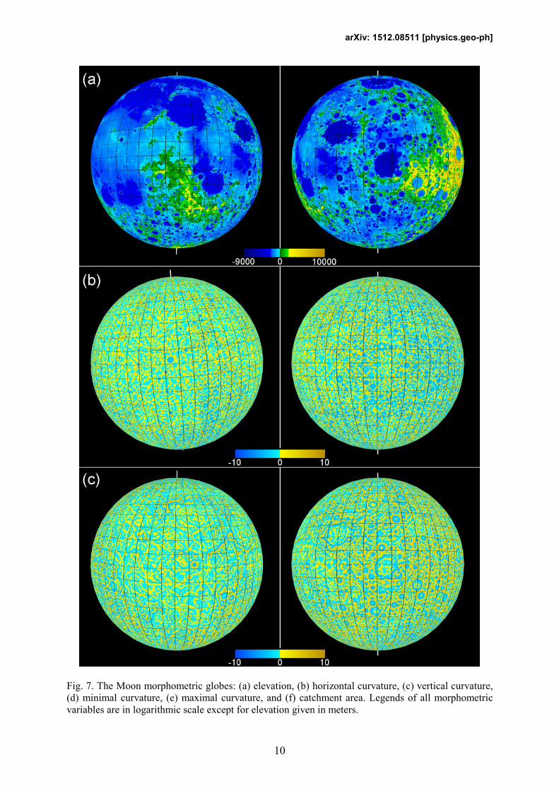
Fig. 7. The Moon morphometric globes: (a) elevation, (b) horizontal curvature, (c) vertical curvature,


variables are in logarithmic scale except for elevation given in meters.


11



12

For the same angular resolution of 15', morphometric globes of the Earth, Mars, and the

Moon have distinct linear resolution (around 27.6 km, 14.8 km, and 7.6 km on the equator,

correspondingly) and scales. Morphometric globes clearly represent peculiarities of planetary

topography, according to the physical and mathematical sense of a particular morphometric

variable.

For example, horizontal curvature delineates areas of flow divergence and convergence

(positive and negative values, correspondingly). These areas relate to spurs of valleys and

ridges (blue and yellow patterns on the kh globes, respectively), which form so-called flow

structures. For the Earth, they are most pronounced in ocean basins (Fig. 5b). On the kh globes

of Mars (Fig. 6b), one can see a system of flow structures incoming to Utopia Planitia from

Nilosyrtis and Protonilus Mensae and Elysium Planitia and Mons. For the Moon, the

horizontal curvature represents cell-like patterns (Fig. 7b) resulting from a predominance of

craters at the global scale.

Vertical curvature is a measure of relative acceleration and deceleration of flows

(positive and negative values, correspondingly). Among other features, the kv globes of the

Earth shows “mega-scarps”, such as edges of continents and mountains (Fig. 5c). On the kv

globes of Mars (Fig. 6c), one can see boundaries of Hellas Planitia, Isidis Planitia, Valles

Marineris, foothills of Olympus Mons, Alba Patera, and so on. On the kv globes of the Moon

(Fig. 7c), one can see well-marked boundaries of Mare Smythii, Mare Crisium, as well as a

plethora of craters.

Catchment area measures an upslope area potentially drained through a point on the

topographic surface. On the CA globes of the Earth (Fig. 5f), low values of CA delineate land

and ocean ridges as white lines (e.g., the Andes and mid-ocean ridges). High values of CA

show land valleys and ocean canyons as black lines, as well as land depressions and ocean

basins as dark areas (e.g., the Mediterranean, Black, and Red Seas). On the CA globes of Mars

(Fig. 6f), one can see the planetary network of valleys and canyons, as well as a large feature,

Solis Planum, and a plethora of smaller depressions, predominantly craters.

Linear artifacts are typical for polar areas of all morphometric globes except for

elevation. They were caused by both reduced accuracy of DEMs in polar areas and some

peculiarities of global DEM processing.

4. Conclusions

We developed the first testing version of the system of virtual morphometric globes for

the Earth, Mars, and the Moon. The system was constructed using Blender, the open-source

software for 3D modeling and visualization. The real-time testing of the developed system

demonstrated its good performance.

The first version of the system is as simple as possible: we used morphometric textures

of low resolution (15'). Morphometric textures of higher resolution (up to 30") and

hierarchical tessellation of the globe surface will be utilized in next versions of the system.

Acknowledgements

The study was supported by RFBR grant 15-07-02484.

References

AGI, 2012–2015. Cesium. Analytical Graphics, Inc., Exton, PA, https://cesium.agi.com

Autin, L., Johnson, G., Hake, J., Olson, A., and Sanner, M., 2012. uPy: A ubiquitous CG

Python API with biological-modeling applications. IEEE Computer Graphics and

Applications, 32: 50–61.

Becker, J.J., Sandwell, D.T., Smith, W.H.F., Braud, J., Binder, B., Depner, J., Fabre, D.,

Factor, J., Ingalls, S., Kim, S.-H., Ladner, R., Marks, K., Nelson, S., Pharaoh, A.,


13

Trimmer, R., von Rosenberg, J., Wallace, G., and Weatherall, P., 2009. Global

bathymetry and elevation data at 30 arc seconds resolution: SRTM30_PLUS. Marine

Geodesy, 32: 355–371.

Blain, J.M., 2012. The Complete Guide to Blender Graphics: Computer Modeling and

Animation. CRC Press, Boca Raton, FL, 389 p.

Blaschke, T., Donert, K., Gossette, F., Kienberger, S., Marani, M., Qureshi, S., and Tiede, D.,

2012. Virtual globes: Serving science and society. Information, 3: 372–390.

Blender Foundation, 2003–2015. Blender. Stichting Blender Foundation, Amsterdam,

https://www.blender.org Chen, A., and Bailey, J. (Eds.), 2011. Virtual Globes in Science. Computers and Geosciences,

37: 1–110.

Cozzi, P., and Ring, K., 2011. 3D Engine Design for Virtual Globes. A K Peters/CRC Press,

Boca Raton, FL, 520 p.

Florinsky, I.V., 1998. Derivation of topographic variables from a digital elevation model

given by a spheroidal trapezoidal grid. International Journal of Geographical

Information Science, 12: 829–852.

Florinsky, I.V., 2008a. Global lineaments: Application of digital terrain modelling. In: Zhou,

Q., Lees, B., and Tang, G.-A. (Eds.), Advances in Digital Terrain Analysis. Springer,

Berlin, pp. 365–382.

Florinsky, I.V., 2008b. Global morphometric maps of Mars, Venus, and the Moon. In: Moore,

A., and Drecki, I. (Eds.), Geospatial Vision: &ew Dimensions in Cartography. Springer,

Berlin, pp. 171–192.

Florinsky, I.V., 2012. Digital Terrain Analysis in Soil Science and Geology. Academic Press,

Amsterdam, 379 p.

Ford, P.G., Pettengill, G., Liu, F., and Quigley, J., 1992. Magellan Global Topography,

Emissivity, Reflectivity, and Slope Data Record. NASA Planetary Data System

Geosciences Node, Washington University, St. Louis, MO, http://pds-

geosciences.wustl.edu/missions/magellan/gxdr/index.htm Google Inc., 2005–2014. Google Earth. Google Inc., http://www.google.com/earth

Gunia, D.A., 2004–2015. Earth3D, http://www.earth3d.org

Guth, P.L., 2012. Automated export of GIS maps to Google Earth: Tool for research and

teaching. Geological Society of America Special Papers, 492: 165–182.

Hansen, C.D., and Johnson, C.R. (Eds.), 2005. The Visualization Handbook. Academic Press,

Amsterdam, 962 p.

Hengl, T., and Reuter, H.I. (Eds.), 2009. Geomorphometry: Concepts, Software, Applications.

Elsevier, Amsterdam, 796 p.

Hess, R., 2010. Blender Foundations: The Essential Guide to Learning Blender 2.6. Focal

Press, Amsterdam, 404 p.

Johnson, G.T., and Hertig, S., 2014. A guide to the visual analysis and communication of

biomolecular structural data. &ature Reviews Molecular Cell Biology, 15: 690–698.

KDE, 2007–2014. Marble. K Desktop Environment, Berlin, https://marble.kde.org

Kent, B.R., 2013. Visualizing astronomical data with Blender. Publications of the

Astronomical Society of the Pacific, 125: 731–748.

Kent, B.R., 2015. 3D Scientific Visualization with Blender®

. Morgan & Claypool Publishers,

San Rafael, CA, 105 p.

Li, Z., Zhu, Q., and Gold, C., 2005. Digital Terrain Modeling: Principles and Methodology.

CRC Press, New York, 323 p.

Lipşa, D.R., Laramee, R.S., Cox, S.J., Roberts, J.C., Walker, R., Borkin, M.A., and Pfister,

H., 2012. Visualization for the physical sciences. Computer Graphics Forum, 31: 2317–

2347.

Mahdavi-Amiri, A., Alderson, T., and Samavati, F., 2015. A survey of Digital Earth.


14

Computers and Graphics, 53: 95–117.

Martz, L.W., and de Jong, E., 1988. CATCH: A Fortran program for measuring catchment

area from digital elevation models. Computers and Geosciences, 14: 627–640.

NASA, 2003–2011. &ASA World Wind. National Aeronautics and Space Administration, http://worldwind.arc.nasa.gov

Neumann, G.A., 2008. Lunar Reconnaissance Orbiter LOLA Instrument Science Data

Archive. NASA PDS Geosciences Node, Washington University, St. Louis, MO, http://pds-geosciences.wustl.edu/missions/lro/lola.htm

Paraskevas, T., 2011. Virtual globes and geological modeling. International Journal of

Geosciences, 2: 648–656.

Phong, B.T., 1975. Illumination for computer generated pictures. Communications of ACM,

18: 311–317.

Ryakhovsky, V., Rundquist, D., Gatinsky, Y., and Chesalova, E., 2003. GIS-project:

Geodynamic globe for global monitoring of geological processes. Geophysical Research

Abstracts, 5: 11645.

Sandwell, D.T., Smith, W.H.F., and Becker, J.J., 2008. SRTM30_PLUS V11. Scripps

Institution of Oceanography, University of California, San Diego, CA, ftp://topex.ucsd.edu/pub/srtm30_plus

Scianna, A., 2013. Building 3D GIS data models using open source software. Applied

Geomatics, 5: 119–132.

SciVis, 2011–2015. BioBlender. Scientific Visualization Unit, Institute of Clinical Physiology

– CNR, Pisa, Italy, http://www.bioblender.eu

Smith, D.E., Zuber, M.T., Solomon, S.C., Phillips, R.J., Head, J.W., Garvin, J.B., Banerdt,

W.B., Muhleman, D.O., Pettengill, G.H., Neumann, G.A., Lemoine, F.G., Abshire, J.B.,

Aharonson, O., Brown, C.D., Hauck, S.A., Ivanov, A.B., McGovern, P.J., Zwally, H.J.,

and Duxbury, T.C., 1999. The global topography of Mars and implications for surface

evolution. Science, 284: 1495–1503.

Smith, D.E., Neumann, G., Arvidson, R.E., Guinness, E.A., and Slavney, S., 2003. Mars

Global Surveyor Laser Altimeter Mission Experiment Gridded Data Record. NASA

Planetary Data System Geosciences Node, Washington University, St. Louis, MO, http://pds-geosciences.wustl.edu/missions/mgs/megdr.html

Smith, D.E., Zuber, M.T., Neumann, G.A., Lemoine, F.G., Mazarico, E., Torrence, M.H.,

McGarry, J.F., Rowlands, D.D., Head, J.W. III, Duxbury, T.H., Aharonson, O., Lucey,

P.G., Robinson, M.S., Barnouin, O.S., Cavanaugh, J.F., Sun, X., Liiva, P., Mao, D.-d.,

Smith, J.C., and Bartels, A.E., 2010. Initial observations from the Lunar Orbiter Laser

Altimeter. Geophysical Research Letters, 37: L18204, doi: 10.1029/2010GL043751.

Tuttle, B.T., Anderson, S., and Huff, R., 2008. Virtual globes: An overview of their history,

uses, and future challenges. Geography Compass, 2: 1478–1505.

Wilson, J.P., and Gallant, J.C. (Eds.), 2000. Terrain Analysis: Principles and Applications.

Wiley, New York, 479 p.

Yu, L., and Gong, P., 2012. Google Earth as a virtual globe tool for Earth science applications

at the global scale: Progress and perspectives. International Journal of Remote Sensing,

33: 3966–3986.

Zhu, L., Sun, J., Li, C., and Zhang, B., 2014. SolidEarth: A new Digital Earth system for the

modeling and visualization of the whole Earth space. Frontiers of Earth Science, 8:

524–539.

Zuber, M., Smith, D.E., and Neumann, G., 1996. Clementine Gravity and Topography Data

Archive. NASA Planetary Data System Geosciences Node, Washington University, St.

Louis, MO, http://pds-geosciences.wustl.edu/missions/clementine/gravtopo.html

development of virtual morphometric globes using blender

Documents