dido optimization of a lunar landing trajectory with ... · naval . postgraduate . school ....

Calhoun: The NPS Institutional Archive

Theses and Dissertations Thesis Collection

2009-09

DIDO optimization of a lunar landing trajectory with

respect to autonomous landing hazard avoidance technology

Francis, Michael R.

Monterey, California. Naval Postgraduate School

http://hdl.handle.net/10945/4508

NAVAL

POSTGRADUATE SCHOOL

MONTEREY, CALIFORNIA

THESIS

DIDO OPTIMIZATION OF A LUNAR LANDING TRAJECTORY WITH RESPECT TO AUTONOMOUS LANDING HAZARD AVOIDANCE TECHNOLOGY

by

Michael R. Francis

September 2009

Thesis Advisor: Daniel W. Bursch Second Reader: James H. Newman

Approved for public release; distribution is unlimited

THIS PAGE INTENTIONALLY LEFT BLANK

i

REPORT DOCUMENTATION PAGE Form Approved OMB No. 0704-0188 Public reporting burden for this collection of information is estimated to average 1 hour per response, including the time for reviewing instruction, searching existing data sources, gathering and maintaining the data needed, and completing and reviewing the collection of information. Send comments regarding this burden estimate or any other aspect of this collection of information, including suggestions for reducing this burden, to Washington headquarters Services, Directorate for Information Operations and Reports, 1215 Jefferson Davis Highway, Suite 1204, Arlington, VA 22202-4302, and to the Office of Management and Budget, Paperwork Reduction Project (0704-0188) Washington DC 20503.

1. AGENCY USE ONLY (Leave blank)

2. REPORT DATE September 2009

3. REPORT TYPE AND DATES COVERED Master’s Thesis

4. TITLE DIDO Optimization of a Lunar Landing Trajectory with Respect to Autonomous Landing Hazard Avoidance Technology

6. Michael R. Francis

5. FUNDING NUMBERS

7. PERFORMING ORGANIZATION NAME(S) AND ADDRESS(ES) Naval Postgraduate School Monterey, CA 93943-5000

8. PERFORMING ORGANIZATION REPORT NUMBER

9. SPONSORING /MONITORING AGENCY NAME(S) AND ADDRESS(ES) N/A

10. SPONSORING/MONITORING AGENCY REPORT NUMBER

11. SUPPLEMENTARY NOTES The views expressed in this thesis are those of the author and do not reflect the official policy or position of the Department of Defense or the U.S. Government.

12a. DISTRIBUTION / AVAILABILITY STATEMENT Approved for public release; distribution is unlimited

12b. DISTRIBUTION CODE

13. ABSTRACT (maximum 200 words)

In this study, the current and expected state of lunar landing technology is assessed. Contrasts are drawn between the technologies used during the Apollo era versus that which will be used in the next decade in an attempt to return to the lunar surface. In particular, one new technology, Autonomous Landing Hazard Avoidance Technology (ALHAT) and one new method, DIDO optimization, are identified and examined. An approach to creating a DIDO optimized lunar landing trajectory which incorporates the ALHAT system is put forth and results are presented. The main objectives of the study are to establish a baseline analysis for the ALHAT lunar landing problem, which can then be followed up with future research, as well as to evaluate DIDO as an optimization tool. Conclusions relating to ALHAT-imposed ConOps (Concept of Operations), sensor scanning methods and DIDO functionality are presented, along with suggested future areas of research.

15. NUMBER OF PAGES

119

14. SUBJECT TERMS DIDO, Optimization, Lunar Landing, Trajectory, Autonomous Landing Hazard Avoidance Technology, Terrain Relative Navigation, Hazard Relative Navigation, Hazard Detection and Avoidance, Lunar Surface Access Module 16. PRICE CODE

17. SECURITY CLASSIFICATION OF REPORT

Unclassified

18. SECURITY CLASSIFICATION OF THIS PAGE

Unclassified

19. SECURITY CLASSIFICATION OF ABSTRACT

Unclassified

20. LIMITATION OF ABSTRACT

UU

NSN 7540-01-280-5500 Standard Form 298 (Rev. 2-89) Prescribed by ANSI Std. 239-18

ii


iii

Approved for public release; distribution is unlimited

DIDO OPTIMIZATION OF A LUNAR LANDING TRAJECTORY WITH RESPECT TO AUTONOMOUS LANDING HAZARD AVOIDANCE

TECHNOLOGY

Michael R. Francis Civilian, Department of Engineering and Applied Sciences

B.S., Massachusetts Institute of Technology, 2006

Submitted in partial fulfillment of the requirements for the degree of

MASTER OF SCIENCE IN SPACE SYSTEMS OPERATIONS

from the

NAVAL POSTGRADUATE SCHOOL September 2009

Author: Michael R. Francis

Approved by: Daniel W. Bursch, Capt., USN (Ret.) Thesis Advisor

James H. Newman, PhD Second Reader

Rudolf Panholzer, PhD Chairman, Department of Space Systems Academic Group

iv


v

ABSTRACT

In this study, the current and expected state of lunar landing technology is

assessed. Contrasts are drawn between the technologies used during the Apollo era

versus that which will be used in the next decade in an attempt to return to the lunar

surface. In particular, one new technology, Autonomous Landing Hazard Avoidance

Technology (ALHAT) and one new method, DIDO optimization, are identified and

examined. An approach to creating a DIDO optimized lunar landing trajectory which

incorporates the ALHAT system is put forth and results are presented. The main

objectives of the study are to establish a baseline analysis for the ALHAT lunar landing

problem, which can then be followed up with future research, as well as to evaluate

DIDO as an optimization tool. Conclusions relating to ALHAT-imposed ConOps

(Concept of Operations), sensor scanning methods and DIDO functionality are presented,

along with suggested future areas of research.

vi


vii

TABLE OF CONTENTS

I. INTRODUCTION........................................................................................................1 A. BACKGROUND ..............................................................................................1 B. PURPOSE.........................................................................................................1 C. RESEARCH QUESTIONS.............................................................................2 D. BENEFITS OF STUDY...................................................................................2 E. SCOPE OF METHODOLOGY .....................................................................2

II. LUNAR TRAJECTORY BACKGROUND RESEARCH .......................................5 A. INTRODUCTION............................................................................................5 B. APOLLO PROGRAM.....................................................................................5

1. Methods.................................................................................................6 a. Reconnaissance.........................................................................6 b. Lunar Descent ...........................................................................8

2. Constraints............................................................................................9 C. RELATED WORK ........................................................................................10

1. Lunar Surface Access Module (LSAM)...........................................10 2. DIDO Optimization ...........................................................................12

a. Cost Functions ........................................................................13 D. CHAPTER SUMMARY................................................................................13

III. ALHAT .......................................................................................................................15 A. INTRODUCTION..........................................................................................15 B. BACKGROUND ............................................................................................15

1. Development .......................................................................................16 2. Function ..............................................................................................20

a. Terrain Relative Navigation (TRN)........................................22 b. Hazard Detection and Avoidance (HDA)...............................22 c. Hazard Relative Navigation (HRN) .......................................22

C. EFFECTS ON LUNAR LANDINGS ...........................................................23 1. New Capabilities.................................................................................23 2. Modified ConOps...............................................................................24

D. CHAPTER SUMMARY................................................................................26

IV. LUNAR LANDER TRAJECTORY MODELING .................................................27 A. INTRODUCTION..........................................................................................27 B. APPROACH...................................................................................................27

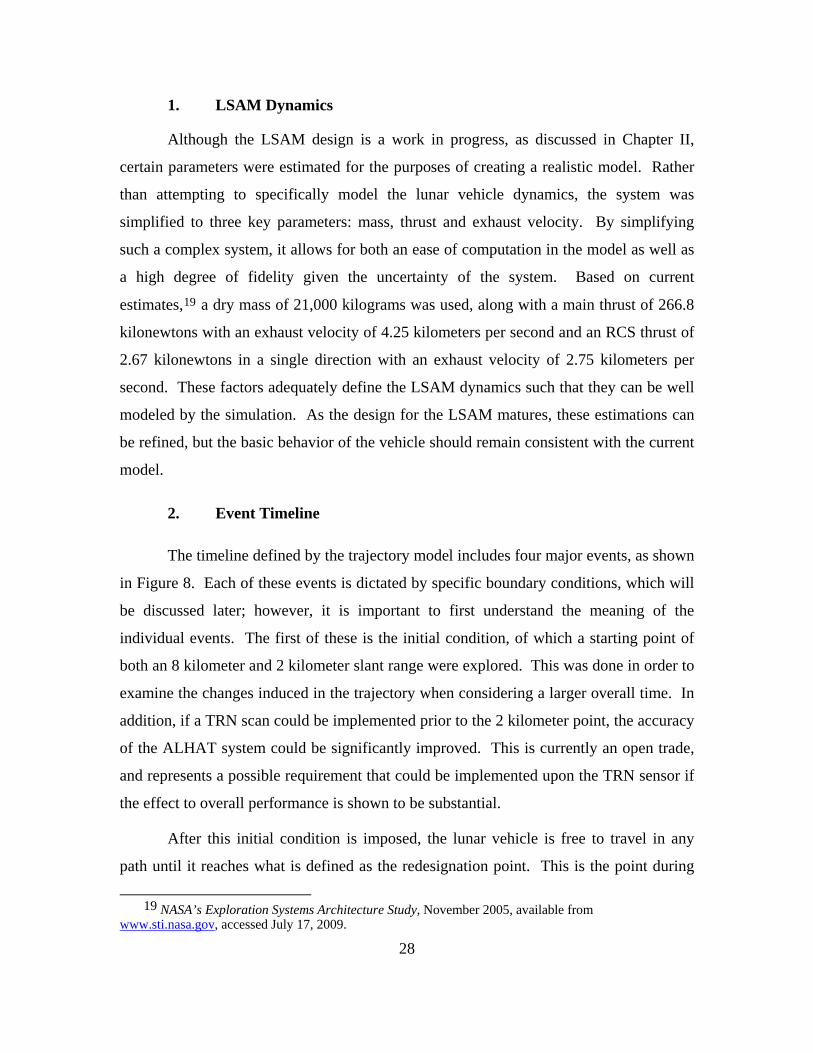
1. LSAM Dynamics ................................................................................28 2. Event Timeline ...................................................................................28 3. Boundary Conditions.........................................................................30 4. Parameters of Interest .......................................................................32

C. COST FUNCTION ........................................................................................34 D. DIDO OPTIMIZATION ...............................................................................35

1. Cost Function File ..............................................................................35

viii

2. Dynamics Function File.....................................................................36 3. Events Function File ..........................................................................36 4. Path Function File..............................................................................37 5. Problem File .......................................................................................37

E. CHAPTER SUMMARY................................................................................38

V. RESEARCH ANALYSIS ..........................................................................................39 A. INTRODUCTION..........................................................................................39 B. CONSTRAINTS.............................................................................................39

1. DIDO ...................................................................................................39 a. State Variables.........................................................................40 b. Mass.........................................................................................40 c. Nodes .......................................................................................41

2. ALHAT ...............................................................................................41 C. TRAJECTORY RESULTS...........................................................................42

1. Initial Condition I ..............................................................................42 2. Initial Condition II.............................................................................46 3. Redesignation Point ...........................................................................50 4. Terminal Descent ...............................................................................54 5. Complete Trajectory..........................................................................58

D. PARAMETER RESULTS ............................................................................62 1. Fuel ......................................................................................................63 2. TRN Sensor.........................................................................................65 3. Path / Safety........................................................................................68

E. CHAPTER SUMMARY................................................................................71

VI. CONCLUSIONS ........................................................................................................73 A. METHODOLOGIES AND RECOMMENDATIONS ...............................73

1. DIDO Utility .......................................................................................73 2. Modeling Parameters.........................................................................74 3. ALHAT Considerations ....................................................................75

B. AREAS FOR FUTURE RESEARCH..........................................................76

LIST OF REFERENCES......................................................................................................79

APPENDIX A: COST FUNCTION FILE ...........................................................................81

APPENDIX B: VERTICAL DYNAMICS FUNCTION FILE ..........................................83

APPENDIX C: HORIZONTAL DYNAMICS FUNCTION FILE ...................................85

APPENDIX D: EVENTS FUNCTION FILE......................................................................87

APPENDIX E: INITIAL CONDITION I PROBLEM FILE ............................................89

APPENDIX F: INITIAL CONDITION II PROBLEM FILE ...........................................91

APPENDIX G: PLOTTING SCRIPT..................................................................................93

INITIAL DISTRIBUTION LIST .......................................................................................101

ix

LIST OF FIGURES

Figure 1. Sea of Tranquility ..............................................................................................7 Figure 2. Apollo Era Lunar Descent Phases......................................................................8 Figure 3. LSAM Reference Design.................................................................................11 Figure 4. Proposed Shackleton Crater Outpost ...............................................................17 Figure 5. Lunar Landing Phases......................................................................................20 Figure 6. Sensor Operational Ranges ..............................................................................21 Figure 7. Approach Phase ConOps .................................................................................25 Figure 8. Event Timeline.................................................................................................30 Figure 9. Parameters of Interest ......................................................................................34 Figure 10. Initial Condition I – Trajectory ........................................................................43 Figure 11. Initial Condition I – Vertical Position..............................................................44 Figure 12. Initial Condition I – Horizontal Position .........................................................45 Figure 13. Initial Condition I – Mass ................................................................................46 Figure 14. Initial Condition II – Trajectory.......................................................................47 Figure 15. Initial Condition II – Vertical Position ............................................................48 Figure 16. Initial Condition II – Horizontal Position ........................................................49 Figure 17. Initial Condition II – Mass...............................................................................50 Figure 18. Redesignation Point – Trajectory.....................................................................51 Figure 19. Redesignation Point – Vertical Position ..........................................................52 Figure 20. Redesignation Point – Horizontal Position ......................................................53 Figure 21. Redesignation Point – Mass.............................................................................54 Figure 22. Terminal Descent – Trajectory ........................................................................55 Figure 23. Terminal Descent – Vertical Position ..............................................................56 Figure 24. Terminal Descent – Horizontal Position..........................................................56 Figure 25. Terminal Descent – Mass.................................................................................57 Figure 26. Complete Initial Condition I Trajectory ..........................................................58 Figure 27. Complete Initial Condition II Trajectory .........................................................59 Figure 28. Complete Initial Condition I Trajectory – Vertical Position ...........................60 Figure 29. Complete Initial Condition II Trajectory – Vertical Position ..........................60 Figure 30. Complete Initial Condition I Trajectory – Horizontal Position .......................61 Figure 31. Complete Initial Condition II Trajectory – Horizontal Position......................61 Figure 32. Complete Initial Condition I Trajectory – Mass ..............................................64 Figure 33. Complete Initial Condition II Trajectory – Mass.............................................65 Figure 34. TRN Sensor Performance ................................................................................66 Figure 35. Initial Condition I – TRN Scan Range.............................................................67 Figure 36. Initial Condition II – TRN Scan Range ...........................................................68 Figure 37. Acceleration Limits for Unconditioned Crewmembers...................................69 Figure 38. Initial Condition I Trajectory – Safety.............................................................70 Figure 39. Initial Condition II Trajectory – Safety ...........................................................71

x


xi

LIST OF TABLES

Table 1. ALHAT Top Level System Requirements ......................................................19 Table 2. ALHAT System Capabilities ...........................................................................24 Table 3. Boundary Conditions .......................................................................................32 Table 4. KPP Evaluation................................................................................................63

xii


xiii

EXECUTIVE SUMMARY

The following study is an analysis of a lunar landing trajectory using an advanced

optimization algorithm known as DIDO, and incorporating Autonomous Landing Hazard

Avoidance Technology (ALHAT). The long duration of time since the United States last

set foot on the moon has caused a substantial gap in associated knowledge, but at the

same time, has allowed for the development of additional technology. Two such

technologies are leveraged in this research: the newly possible DIDO optimization

method and ALHAT. DIDO optimization employs Legendre Polynomials to create an

approximation of variables over multiple nodes as opposed to the use of a fixed order

polynomial or single node perpetuation of state variables. This creates more continuity in

the optimization and allows for a more complete result overall. ALHAT uses a series of

sensors as well as a priori knowledge of the lunar surface to provide precision guidance

with respect to landing hazards. This allows the lunar landing vehicle to position itself

near terrain objects of interest without threatening the safety of the crew or the vehicle.

The incorporation of these new technologies necessitates an analysis of their

impact on the foundation of knowledge previously gathered, primarily during the Apollo

era. This study provides a baseline for this exploration by analyzing a lunar landing

trajectory using two distinct initial conditions and employing a DIDO optimization

method. In documenting this approach, creating the necessary code to run the

optimization and analyzing the results, this study hopes to provide insight into key

questions. The utility of DIDO as an optimization tool is examined. The effects of

incorporating the ALHAT system into the lunar vehicle on the resulting trajectory are

studied as well. Finally, conclusions and recommendations are drawn with respect to

possible changes in ConOps, ALHAT open trades, the usefulness of DIDO and areas for

future research.

xiv


xv

ACKNOWLEDGMENTS

I would like to first thank all of my family and friends whose gentle, yet constant,

reminders of my thesis responsibilities helped to eventually produce the following results.

I would also like to thank my thesis advisor, Professor Daniel Bursch, Capt, USN

(Ret.) for his guidance and patience, my academic advisor, Professor Mark Rhoades for

his diligence in this process, as well as Professor Jim Newman, PhD, for his expertise and

support, Professor I. Michael Ross, PhD, for his assistance with DIDO and Ron Sostaric

and Chirold Epp, PhD, for sharing their knowledge of ALHAT.

Finally, I would like to thank the NPS MSSSO-DL 2008 cohort, who spent many

long nights and early mornings communicating via unreliable technology in what was

hopefully a successful effort to improve it for future users.

xvi


1

I. INTRODUCTION

A. BACKGROUND

The United States has not landed on the moon since the Apollo 17 mission on

December 7, 1972. In accordance with recent governmental actions and presidential

decrees, NASA looks to return to the lunar surface for the first time in over 35 years.

This exceptional absence has allowed certain expertise to fade; however, it has also

provided sufficient time for the development of new technologies that may help to ensure

a safe and extremely successful lunar mission to occur within the target date of 2020.

Autonomous Landing and Hazard Avoidance Technology (ALHAT) is an example of

such technological progress. By successfully and accurately calculating lunar approach

trajectories and adjusting these trajectories to take into account hazardous terrain, lunar

missions will be capable of safely landing in proximity to large obstructions or in

otherwise dangerous terrain. This will aid in the establishment of a useful and efficient

lunar base by reducing the restriction of landing site location and increasing overall

safety. Analysis provided in this thesis will examine the benefits of such an optimized

trajectory and explore the differences induced by incorporating such technology from

previous lunar missions. By employing a given cost function that accurately reflects

desired capabilities, the developing ALHAT trade space can be explored. In addition,

implementation of an advanced optimization method known as DIDO will provide

unique results that have, by in large, not been previously examined. Conclusions will be

made and recommendations for future research suggested as deemed necessary.

B. PURPOSE

This research will be used to aid in the ongoing development of the ALHAT

system with respect to both requirements and Concepts of Operation (ConOps). An

exploration of the possible trade space will help to further define sensor requirements as

well as determine procedures for actual use. In addition, the results will help to

investigate possible alterations to current lunar landing procedures. Changes in protocol

2

can be made to take full advantage of the new capabilities provided by the ALHAT

system. Discrepancies between results and current practices will highlight areas

requiring additional research in order to completely understand the effects of ALHAT. In

addition, the usefulness of DIDO as a system analysis method will be explored and

evaluated.

C. RESEARCH QUESTIONS

There are two primary research questions that will be answered in the course of

this document. First, the utility of implementing a DIDO optimization for the purposes of

studying a fuel optimized lunar landing trajectory with respect to the current trade space

of both the proposed lunar vehicle and ALHAT system will be evaluated. This will allow

for an investigation of the applicable parameters with regard to lunar landing missions.

Secondly, the effects of the ALHAT system on this optimal trajectory will be explored to

assist in recommendations for system requirements and mission ConOps that could prove

beneficial to both systems.

D. BENEFITS OF STUDY

This thesis will highlight specific areas that should be further researched with

regards to future lunar landings, particularly in regards to mission ConOps. In addition, it

will explore the utility of ALHAT and the DIDO optimization method, and provide an

initial framework describing the role these new technologies may play, as well as the

effects they may have on current and future analysis. Finally, results will provide further

insight into developing requirements for the ALHAT system as a whole.

E. SCOPE OF METHODOLOGY

This document will focus on a DIDO optimization of student-created code written

in Matlab. The code will be built from analysis of a lunar landing trajectory employing

the expected capabilities of the future lunar vehicle, as well as the ALHAT system. The

developed trajectories will be evaluated with respect to relevant key parameters. Lunar

vehicle data will be acquired from NASA, and information regarding ALHAT will be

3

obtained from contacts at JPL and the NASA Johnson Space Center. The thesis will not

attempt to be an exhaustive analysis of the ALHAT system as it relates to lunar landings,

but rather will provide a starting point for future research in this field.

4


5

II. LUNAR TRAJECTORY BACKGROUND RESEARCH

A. INTRODUCTION

In order to effectively assess both the optimal trajectory for the new era of lunar

exploration as well as the effects of the ALHAT system on this trajectory, it is important

to understand both how previous lunar analysis was originally conceived, and what type

of progress has been achieved since. Simple analysis of lunar trajectories has existed for

decades, so in order to comprehend the changes made by introducing such complexities

as the ALHAT system, one must first have a clear notion of the baseline analysis and

what motivated it. In addition, to apply these complexities in a manner accurately

reflecting real life, a clear concept of the newly developed methods and capabilities that

will be employed is required. This includes an understanding of both the trajectories

employed during the original Apollo missions as well as the newly proposed Crew

Exploration Vehicle (CEV) technology and DIDO optimization method that will be

applied.

B. APOLLO PROGRAM

The Apollo program consisted of a series of missions designed to continuously

apply and test all of the technologies and procedures that would be necessary for a

successful lunar landing. The program culminated with six successful lunar landings.

Throughout this process, numerous tests were conducted and procedures developed that

attempted to ensure both the safety of the astronauts and success of the mission. In order

to accomplish NASA’s goals of returning to the lunar surface by 2020, it is essential that

we incorporate these lessons into our new methodology. In order to do so, a proper

understanding of both the procedures employed during the Apollo era and constraints it

faced is required.

6

1. Methods

Neil Armstrong first set foot on the lunar surface on July 20, 1969, during the

Apollo 11 mission. It was not solely this mission, however, that was required to achieve

such a momentous event in human history. Previous missions had been carried out in

order to test various aspects of the eventual lunar landing maneuver and to perform

reconnaissance on plausible landing sites that appeared relatively safe. Much of the

guidance calculations were performed manually and landing sites were selected based

primarily on supposed safety and ease of landing. These selection criteria are considered

to represent a more conservative approach than what NASA would like to achieve in

2020.

a. Reconnaissance

Apollo missions eight through ten were all manned missions involving

lunar orbital trajectories. During these missions, a number of parameters were tested and

a great deal of data was collected, which would later facilitate lunar landing. In

particular, continual reconnaissance was performed in order to select an appropriate

landing site for the Apollo 11 crew. The site, Mare Tranquillitatis, or the Sea of

Tranquility, shown in Figure 1, was chosen primarily with regard to the expected ease of

landing and relative safety, as predicted from generally gentle and sparse geographical

features. From photographs, this area appeared relatively smooth and level, providing

what hoped to be a simple landing process.

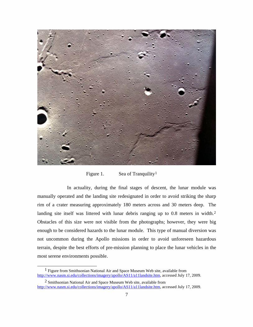
Figure 1. Sea of Tranquility1

In actuality, during the final stages of descent, the lunar module was

manually operated and the landing site redesignated in order to avoid striking the sharp

rim of a crater measuring approximately 180 meters across and 30 meters deep. The

landing site itself was littered with lunar debris ranging up to 0.8 meters in width.2

Obstacles of this size were not visible from the photographs; however, they were big

enough to be considered hazards to the lunar module. This type of manual diversion was

not uncommon during the Apollo missions in order to avoid unforeseen hazardous

terrain, despite the best efforts of pre-mission planning to place the lunar vehicles in the

most serene environments possible.

1 Figure from Smithsonian National Air and Space Museum Web site, available from

http://www.nasm.si.edu/collections/imagery/apollo/AS11/a11landsite.htm, accessed July 17, 2009.

2 Smithsonian National Air and Space Museum Web site, available from http://www.nasm.si.edu/collections/imagery/apollo/AS11/a11landsite.htm, accessed July 17, 2009.

7

http://www.nasm.si.edu/collections/imagery/apollo/AS11/a11landsite.htm


b. Lunar Descent

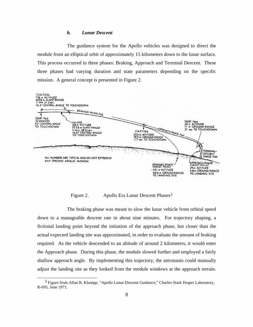
The guidance system for the Apollo vehicles was designed to direct the

module from an elliptical orbit of approximately 15 kilometers down to the lunar surface.

This process occurred in three phases: Braking, Approach and Terminal Descent. These

three phases had varying duration and state parameters depending on the specific

mission. A general concept is presented in Figure 2.

Figure 2. Apollo Era Lunar Descent Phases3

The braking phase was meant to slow the lunar vehicle from orbital speed

down to a manageable descent rate in about nine minutes. For trajectory shaping, a

fictional landing point beyond the initiation of the approach phase, but closer than the

actual expected landing site was approximated, in order to evaluate the amount of braking

required. As the vehicle descended to an altitude of around 2 kilometers, it would enter

the Approach phase. During this phase, the module slowed further and employed a fairly

shallow approach angle. By implementing this trajectory, the astronauts could manually

adjust the landing site as they looked from the module windows at the approach terrain.

3 Figure from Allan R. Klumpp, “Apollo Lunar-Descent Guidance,” Charles Stark Draper Laboratory,

R-695, June 1971.

8

9

When an acceptable landing site was found and the module had reached the appropriate

velocities, it entered Terminal Descent phase. This phase was a relatively steep drop for

roughly the final 30 meters. Although the guidance algorithm continued to target the

desired landing site, it was not expected that the vehicle would achieve it exactly, due to

delays in processing and overall accuracy of control systems.4

2. Constraints

Although the Apollo lunar landing missions were highly successful, the landings

were bound by a number of constraints. First, the overall landing site location was

restricted to areas that were deemed suitably safe. Smooth and level terrain were key

features targeted prior to the mission in order to ensure a safe landing site could be found

during the actual approach. If there were too many hazards apparent during the landing,

an abort was achievable at the cost of mission success. This constraint constantly kept in

check the NASA scientist’s and mission planner’s desires to land in proximity to sites of

high scientific interest, including craters and other large debris. Although these features

were desirable in the sense of scientific inquiry, they were exactly what were to be

avoided in order to facilitate safe landing processes. In addition, this constraint required

extensive research with respect to the landing site prior to the mission in order to avoid an

abort.

Along with this limitation in regards to location, there were additional factors that

constrained Apollo landing sites, due to the necessity of manual redesignation of sites in

order to avoid smaller hazards that could not be detected from previous reconnaissance.

This implied, first off, that landings must occur in sufficient lighting to allow the

astronauts to detect such hazards, requiring solar incidence angles approximating dawn,

about 7-20 degrees. Secondly, approach vectors had to be relatively shallow such that the

view from the lunar module window to the expected landing site was not obstructed, on

4 Ronald Sostaric and Jeremy Rea, Powered Descent Guidance Methods for the Moon and Mars.

Johnson Space Center, Houston, TX.

10

the order of 15 degrees.5 These factors created limitations on the time and location of the

desired landing site, as well as the approach trajectory used to arrive there.

C. RELATED WORK

In addition to the lessons learned from the Apollo era missions, it is important to

incorporate the developments that have taken place over the past four decades since we

traveled to the moon. These newly designed methods and technologies will allow NASA

astronauts to overcome many of the constraints seen during the Apollo missions. In this

way, new capabilities can be employed to supplement practiced procedures in order to

facilitate an improved approach toward lunar exploration.

1. Lunar Surface Access Module (LSAM)

Perhaps the most important new technology with regards to lunar exploration is

the Lunar Surface Access Module (LSAM). The LSAM contract, as a subset of the Crew

Exploration Vehicle (CEV), which is being designed and developed by Lockheed Martin,

has not yet been awarded, though initial baseline concepts have arisen from various

sources. The CEV is meant to replace the shuttle, which will be retired in 2010. In the

interim, all NASA flights will be reliant on the Russian space vehicle, the Soyuz. This

process is meant to build on our first four decades of space flight experience by

incorporating state-of-the-art technological developments in a new space vehicle, an

upgrade that has been deemed vital, particularly in light of the recent shuttle failures.

While development of the LSAM is still under way, NASA did put forth a

reference design in 2005,6 the result of a development team’s efforts to conduct major

trade studies and apply lessons learned from the Apollo program. This reference design

is shown in Figure 3. It is composed of both an ascent and descent stage single cabin,

capable of supporting four astronauts up to seven days on the lunar surface. The LSAM

provides 31.8 cubic meters of pressurized volume for the crew, and features an easily

5 Chirold Epp et al., Autonomous Landing and Hazard Avoidance Technology (ALHAT), Johnson

Space Center, Houston, TX.

6 NASA’s Exploration Systems Architecture Study, November 2005, available from www.sti.nasa.gov, accessed July 17, 2009.

http://www.sti.nasa.gov/

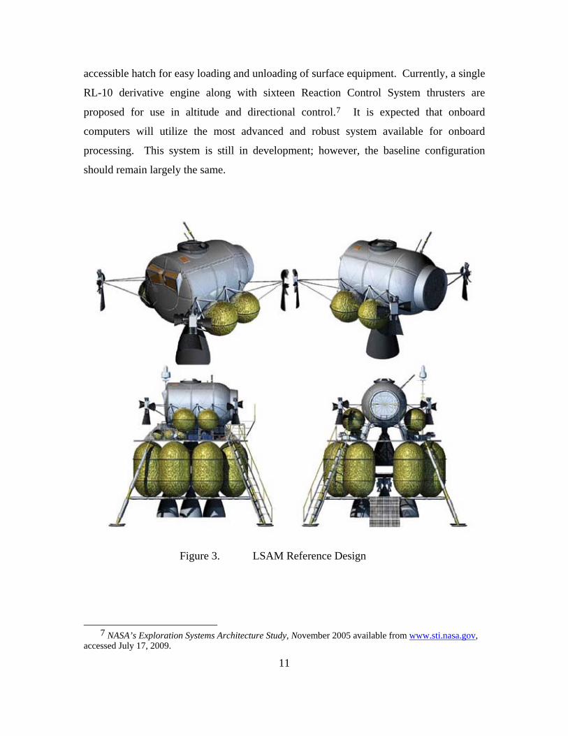
accessible hatch for easy loading and unloading of surface equipment. Currently, a single

RL-10 derivative engine along with sixteen Reaction Control System thrusters are

proposed for use in altitude and directional control.7 It is expected that onboard

computers will utilize the most advanced and robust system available for onboard

processing. This system is still in development; however, the baseline configuration

should remain largely the same.

Figure 3. LSAM Reference Design

7 NASA’s Exploration Systems Architecture Study, November 2005 available from www.sti.nasa.gov,

accessed July 17, 2009.

11


12

2. DIDO Optimization

One of the greatest gains in technological development since man first traveled to

the moon is with respect to the computer processing capabilities. Computers have

improved exponentially in processing speed and ability, allowing complex computations

to be completed quickly and efficiently without imposing a significant drain on resources.

One example of this improvement is in the field of optimization analysis. In order to

fully analyze a complex system involving numerous dependent variables, an effective

algorithm must be employed. In the past, this was an extremely difficult task, and

indirect, approximate methods were utilized in order to allow solutions to be found.

These methods still required a fair knowledge of the expected outcome, however, and

often relied upon extremely difficult analytical equations in order to reach a convergent

solution.8 With the emergence of such improved processing power and the application of

new methods, more direct approaches may be employed to achieve high accuracy without

the associated difficulties in computation or pre-existing knowledge of the solution. An

example of such an approach is DIDO9 optimization.

DIDO relies on the Legendre Pseudospectral Method, which has been developed

and employed primarily in fluid flow modeling. This method employs Legendre

Polynomials to create an approximation of variables over multiple nodes as opposed to

the use of a fixed order polynomial. This allows, despite discontinuities in the governing

equations, a solution to be attained with high accuracy which also satisfies the imposed

optimization criterion, where most direct methods do not.10 The result is a method of

solving a complex dynamic optimization problem without an a priori knowledge of the

8 M. Ross and F. Fahroo, A Perspective on Methods for Trajectory Optimization, AIAA/AAS

Astrodynamics Specialist Conf., Monterey, 2002.

9 It should be noted that DIDO is not actually an acronym. The method is named for Queen Dido of Carthage (circa 850BC) who was the first person known to have solved a dynamic optimization problem. The method name appears in all caps by convention.

10 M. Ross and F. Fahroo, A Perspective on Methods for Trajectory Optimization, AIAA/AAS Astrodynamics Specialist Conf., Monterey, 2002.

13

solution or incredibly complex analytic computations. This is exactly the type of method

required to optimize a problem as complex as an examination of the trade space for lunar

landing.

a. Cost Functions

Although the particulars of the DIDO algorithm which are used to

optimize the user defined problem are private, and therefore not available, the scripts

employed by the user to define the problem and guide the optimization are. At the heart

of the DIDO optimization method, as it applies to the lunar landing problem, is the cost

function. This is what will be used to drive the parameters of interest involved in the

trade space simultaneously. By creating a cost function that accurately relates the overall

value of different lunar landing parameters such as fuel usage, landing accuracy and

vehicle safety, one can extrapolate the resulting modifications and requirements

necessary to input parameters such as sensor scanning time, approach angle, altitude and

velocity, vehicle tolerances and desired fuel reserves. By altering this cost function and

studying the effects to these parameters, one can explore the desired trade space in order

to identify system configurations of interest, as well as sensitivities to system parameters.

An exploration and analysis of this data is at the core of this thesis and will be explained

in greater detail in Chapters IV and V. The importance of DIDO to this process,

however, must be emphasized; such an endeavor would not have been feasible prior to its

development.

D. CHAPTER SUMMARY

A great deal of research has been done with respect to lunar exploration,

beginning with preparation and experience resulting from the Apollo missions,

continuing with technological progress in related areas such as computer processing and

optimization methods, and ongoing with current new developments of advanced lunar

landing vehicles such as the LSAM. With this background of understanding available, it

is important to consider the lessons from those that have gone before, rather than

attempting to resolve a problem where a solution already exists. It is with this philosophy

14

in mind that progress towards a return to the lunar surface is made, and reflects the

processes used in this document of anchoring the analysis in past experience, while

introducing new elements such as ALHAT as a possible method to alleviate past

constraints.

15

III. ALHAT

A. INTRODUCTION

Autonomous Landing and Hazard Avoidance Technology (ALHAT) will allow

spacecraft to land more precisely and in locations of greater interest than ever before.

This technology is being developed in order to increase the capabilities of both

autonomous and manned vehicles in their quest to reach desired, though potentially

dangerous, landing sites. By incorporating the human techniques demonstrated during

the Apollo missions into a technological system of sensors and controls, astronauts and

rovers alike will be given a greater capacity to understand the environment in which they

are attempting to land and to do so safely, while still locating themselves in close

proximity to areas of high interest or importance.

Such a system requires a great deal of testing and understanding if it is to

supplement human operators’ decisions reliably, and if we are to trust the lives of

astronauts and successes of unmanned missions to its capabilities. Though ALHAT

operates autonomously, during manned missions it is meant to facilitate the decisions of

human operators, rather than replace them, and so it is important to have a thorough

comprehension of the processes it uses to do so. As such, an understanding of the

development stages of ALHAT is required, along with the vast trade space under which it

continues to be designed. In addition, its functionality and how it relates to lunar landing

procedures should be examined. From this basic background, an examination of the new

capabilities ALHAT offers and alterations to previous ConOps will be possible.

B. BACKGROUND

To understand the current and possible future capabilities that ALHAT provides,

it is important to have a concept of what motivated the development of this technology,

as well as a definition of the requirements that drove the vast trade space. Keep in mind

that some of these capabilities are still in development, and trades against exact

16

specifications are still being examined such that final ConOps have not yet been written;

the possibilities, however, are already apparent.

1. Development

NASA is currently committed to returning to the lunar surface by 2020. The

NASA Authorization Act of 2005 stated that NASA shall establish a program to develop

a sustained human presence on the moon, including a robust precursor program to

promote exploration, science, commerce and U.S. preeminence in space, and as a

stepping stone to future exploration of Mars and other destinations.11 It is clear from such

documentation that NASA is sincere in this mission, and, as such, has put plans in motion

to develop the necessary technology to get there.

In 2006, NASA released another series of documents that put forth a method to

accomplish the stated tasks. The Global Exploration Strategy and Lunar Architecture

was developed in order to answer the questions of why we should focus on a return to the

moon, and what we might do when we arrived. The answer to the first question is

important, though largely outside the scope of this document, and so will not be

discussed. Included in the answer to the second, however, is the looming question of just

what technologies and procedures will be necessary to accomplish all that we desire upon

arrival.

NASA’s Lunar Architecture includes proposed permanent outposts on one or both

of the lunar poles. The southern outpost location is proposed as Shackleton Crater, which

as shown in Figure 4, is a large area with a good deal of hazardous terrain—an area that

the Apollo missions would not have considered a feasible landing site. This architecture,

then, implies advancement in our current capabilities. Thus, the need for ALHAT, as

well as numerous other new technologies, arose.

11 IEEEAC paper #1643, Version 5, Updated December 17, 2007.

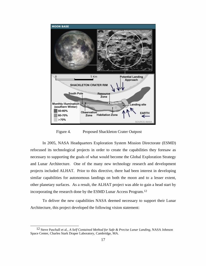
Figure 4. Proposed Shackleton Crater Outpost

In 2005, NASA Headquarters Exploration System Mission Directorate (ESMD)

refocused its technological projects in order to create the capabilities they foresaw as

necessary to supporting the goals of what would become the Global Exploration Strategy

and Lunar Architecture. One of the many new technology research and development

projects included ALHAT. Prior to this directive, there had been interest in developing

similar capabilities for autonomous landings on both the moon and to a lesser extent,

other planetary surfaces. As a result, the ALHAT project was able to gain a head start by

incorporating the research done by the ESMD Lunar Access Program.12

To deliver the new capabilities NASA deemed necessary to support their Lunar

Architecture, this project developed the following vision statement:

12 Steve Paschall et al., A Self Contained Method for Safe & Precise Lunar Landing, NASA Johnson

Space Center, Charles Stark Draper Laboratory, Cambridge, MA.

17

18

Develop and mature to a TRL 6 an autonomous lunar landing GN&C and

sensing system for crewed, cargo, and robotic lunar descent vehicles. The

ALHAT System will be capable of identifying and avoiding surface

hazards to enable a safe precision landing to within tens of meters of

certified and designated landing sites anywhere on the Moon under any

lighting conditions.13

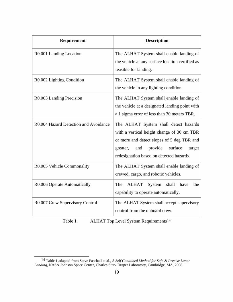
Top level requirements were developed in order to guide the program with measurable

directives. These top level system requirements are shown in Table 1.

From these beginnings, the ALHAT project had a basis of research from which to

build, a purpose in the form of a problem to solve and initial requirements derived from a

cursory understanding of the problem. As can be noted from examining Table 1, some of

the specific high level requirements values were initially noted as TBR (To Be Resolved),

indicating there was not a complete understanding of the precise requirements for lunar

landing (which had not yet been developed by NASA), the capabilities that could be

obtained, or the trade space that would be examined, and so there was room left for

adjustment. From these requirements, however, one can begin to see the capabilities that

such technology will allow.


Space Center, Charles Stark Draper Laboratory, Cambridge, MA.

19

Requirement Description

R0.001 Landing Location The ALHAT System shall enable landing of

the vehicle at any surface location certified as

feasible for landing.

R0.002 Lighting Condition The ALHAT System shall enable landing of

the vehicle in any lighting condition.

R0.003 Landing Precision The ALHAT System shall enable landing of

the vehicle at a designated landing point with

a 1 sigma error of less than 30 meters TBR.

R0.004 Hazard Detection and Avoidance The ALHAT System shall detect hazards

with a vertical height change of 30 cm TBR

or more and detect slopes of 5 deg TBR and

greater, and provide surface target

redesignation based on detected hazards.

R0.005 Vehicle Commonality The ALHAT System shall enable landing of

crewed, cargo, and robotic vehicles.

R0.006 Operate Automatically The ALHAT System shall have the

capability to operate automatically.

R0.007 Crew Supervisory Control The ALHAT System shall accept supervisory

control from the onboard crew.

Table 1. ALHAT Top Level System Requirements14

14 Table 1 adapted from Steve Paschall et al., A Self Contained Method for Safe & Precise Lunar

Landing, NASA Johnson Space Center, Charles Stark Draper Laboratory, Cambridge, MA, 2008.

2. Function

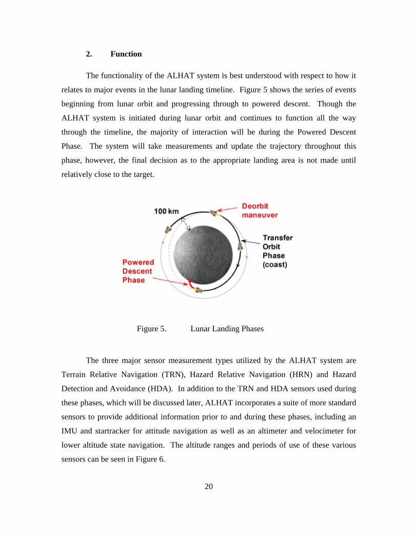
The functionality of the ALHAT system is best understood with respect to how it

relates to major events in the lunar landing timeline. Figure 5 shows the series of events

beginning from lunar orbit and progressing through to powered descent. Though the

ALHAT system is initiated during lunar orbit and continues to function all the way

through the timeline, the majority of interaction will be during the Powered Descent

Phase. The system will take measurements and update the trajectory throughout this

phase, however, the final decision as to the appropriate landing area is not made until

relatively close to the target.

Figure 5. Lunar Landing Phases

The three major sensor measurement types utilized by the ALHAT system are

Terrain Relative Navigation (TRN), Hazard Relative Navigation (HRN) and Hazard

Detection and Avoidance (HDA). In addition to the TRN and HDA sensors used during

these phases, which will be discussed later, ALHAT incorporates a suite of more standard

sensors to provide additional information prior to and during these phases, including an

IMU and startracker for attitude navigation as well as an altimeter and velocimeter for

lower altitude state navigation. The altitude ranges and periods of use of these various

sensors can be seen in Figure 6.

20

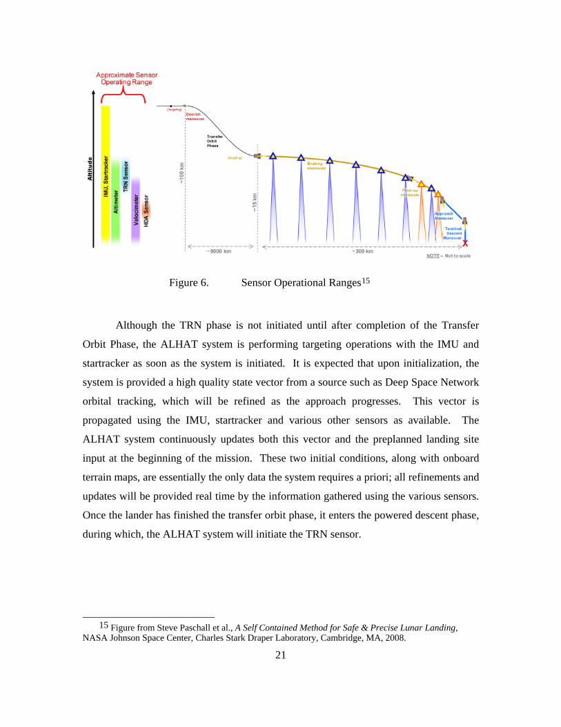
Figure 6. Sensor Operational Ranges15

Although the TRN phase is not initiated until after completion of the Transfer

Orbit Phase, the ALHAT system is performing targeting operations with the IMU and

startracker as soon as the system is initiated. It is expected that upon initialization, the

system is provided a high quality state vector from a source such as Deep Space Network

orbital tracking, which will be refined as the approach progresses. This vector is

propagated using the IMU, startracker and various other sensors as available. The

ALHAT system continuously updates both this vector and the preplanned landing site

input at the beginning of the mission. These two initial conditions, along with onboard

terrain maps, are essentially the only data the system requires a priori; all refinements and

updates will be provided real time by the information gathered using the various sensors.

Once the lander has finished the transfer orbit phase, it enters the powered descent phase,

during which, the ALHAT system will initiate the TRN sensor.

15 Figure from Steve Paschall et al., A Self Contained Method for Safe & Precise Lunar Landing,

NASA Johnson Space Center, Charles Stark Draper Laboratory, Cambridge, MA, 2008.

21

22

a. Terrain Relative Navigation (TRN)

During the TRN phase, the IMU and startracker will continue to operate.

However, the system will also begin to collect information from the altimeter, TRN

position sensor and eventually, the velocimeter. During the TRN phase, the sensors

provide a measurement of the terrain, as well as the position of the vehicle, and compare

it to the onboard terrain maps obtained from lunar reconnaissance data. This phase is

significant, as it is the first time the state vector can be updated with local terrain data.

This update will account for error in the location of the vehicle’s position relative to the

landing target. Reduction of this error is extremely important in order to achieve the high

degree of accuracy required by the ALHAT mission. As the vehicle progresses through

powered descent, a pitch-up maneuver is executed at approximately 1.5 kilometers from

the landing site. At this time, the system enters the Hazard Detection and Avoidance

phase.

b. Hazard Detection and Avoidance (HDA)

During the HAD phase, the expected landing site is examined and

evaluated, and a new site may be selected. Using the HDA sensor, the ALHAT system

examines the initial landing target terrain, as well as the surrounding area, for potential

hazards and creates a Digital Elevation Map (DEM) which identifies safe landing areas

that can be reached. The system then reports its findings to the onboard crew and awaits

a decision, or in the case of an autonomous system, follows a preprogrammed logic. The

crew or the autonomous system select a safe site based on the DEM and other mission

constraints, and then the vehicle guidance system commands the vessel to the selected

safe site. When the final landing site has been determined, the system initiates Hazard

Relative Navigation.

c. Hazard Relative Navigation (HRN)

In the HRN phase, the vehicle’s position relative to the landing target is

further refined using the HDA sensor. The major difference between this phase and the

TRN phase is that vehicle location data is compared to in-flight HDA generated terrain

23

maps as opposed to onboard mission maps provided prior to launch. The maps created

by the HDA sensor are extremely accurate due to the far greater proximity of the sensor

to the ground. This allows for an extremely precise knowledge of the vehicle’s position

relative to the landing target as well as the associated hazards within this site. Smaller

hazards that were not detected on the onboard mission maps are now apparent due to the

much higher resolution. This highly accurate data allows the lander to achieve the safest

and most precise landing possible.

C. EFFECTS ON LUNAR LANDINGS

With development of the ALHAT system, new capabilities and ConOps are

available. Improvements over the methods used during the Apollo era are possible due to

the advancement in associated technological systems, such as the LSAM, as well as the

introduction of ALHAT. In conjunction with these advancements, new ConOps are

possible which will ideally take full advantage of these new features and capabilities.

NASA believes that this will enable them to land vehicles safer and in locations of

greater interest.

1. New Capabilities

ALHAT provides a number of new capabilities to both manned and autonomous

landing vehicles. One such assessment of these new abilities is as follows:

The ALHAT System employs an Autonomous Flight Manager (AFM) which supervises the GNC and sensor systems in nominal situations and monitors/replans in off-nominal situations. For crewed vehicles, the AFM replaces the heavy ground involvement required by Apollo, and also reduces the onboard crew workload and error probability. This allows the crew to focus more on the objectives of landing as opposed to detailed procedural steps. For robotic vehicles, the AFM replaces the crew functions and allows the vehicle to land safely and precisely (independently or without heavy ground operator involvement).16


Space Center, Charles Stark Draper Laboratory, Cambridge, MA, 2008.

24

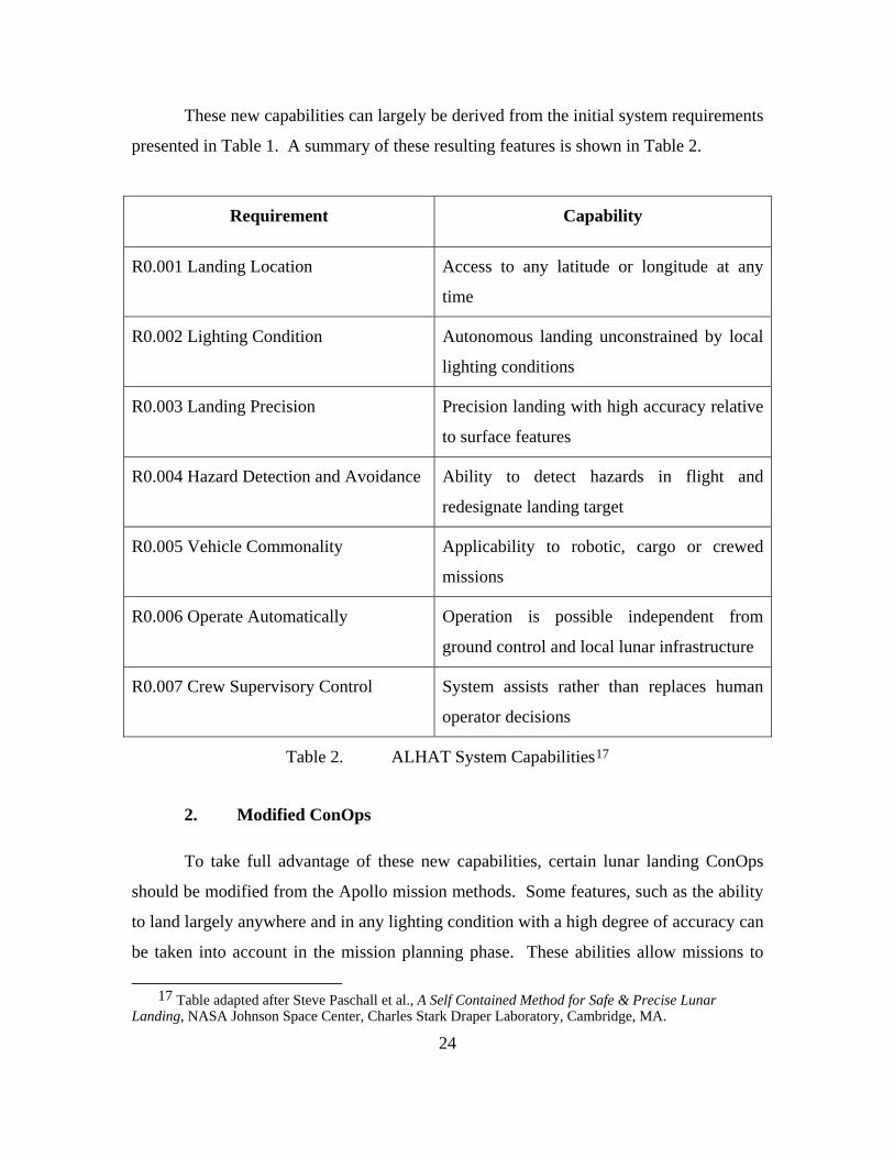
These new capabilities can largely be derived from the initial system requirements

presented in Table 1. A summary of these resulting features is shown in Table 2.

Requirement Capability

R0.001 Landing Location Access to any latitude or longitude at any

time

R0.002 Lighting Condition Autonomous landing unconstrained by local

lighting conditions

R0.003 Landing Precision Precision landing with high accuracy relative

to surface features

R0.004 Hazard Detection and Avoidance Ability to detect hazards in flight and

redesignate landing target

R0.005 Vehicle Commonality Applicability to robotic, cargo or crewed

missions

R0.006 Operate Automatically Operation is possible independent from

ground control and local lunar infrastructure

R0.007 Crew Supervisory Control System assists rather than replaces human

operator decisions

Table 2. ALHAT System Capabilities17

2. Modified ConOps

To take full advantage of these new capabilities, certain lunar landing ConOps

should be modified from the Apollo mission methods. Some features, such as the ability

to land largely anywhere and in any lighting condition with a high degree of accuracy can

be taken into account in the mission planning phase. These abilities allow missions to

17 Table adapted after Steve Paschall et al., A Self Contained Method for Safe & Precise Lunar

Landing, NASA Johnson Space Center, Charles Stark Draper Laboratory, Cambridge, MA.

land in areas that are of high interest, while maintaining a desired level of safety. Such

flexibility is essential to the proposed Lunar Architecture, especially if we are to establish

outposts in areas such as Shackleton Crater. Other new features suggest a new method of

lunar landing procedures.

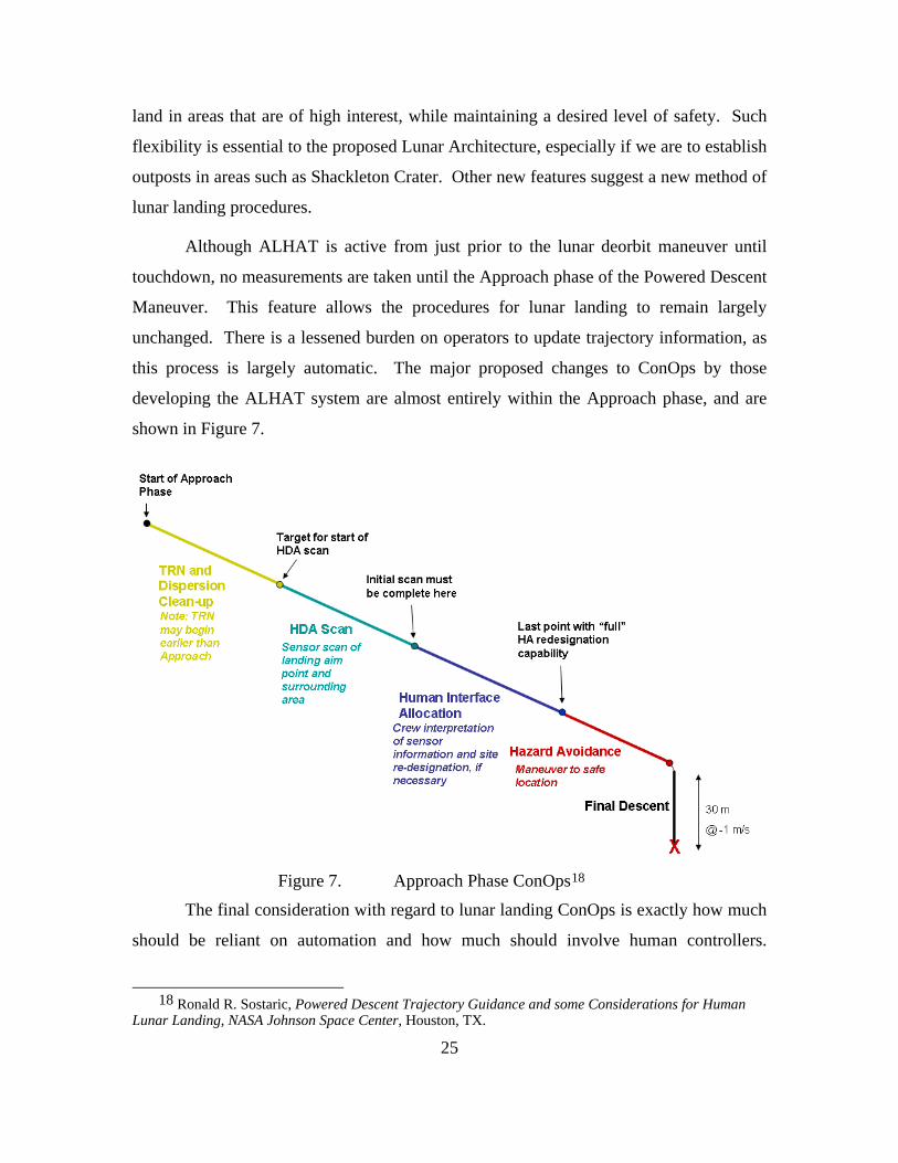
Although ALHAT is active from just prior to the lunar deorbit maneuver until

touchdown, no measurements are taken until the Approach phase of the Powered Descent

Maneuver. This feature allows the procedures for lunar landing to remain largely

unchanged. There is a lessened burden on operators to update trajectory information, as

this process is largely automatic. The major proposed changes to ConOps by those

developing the ALHAT system are almost entirely within the Approach phase, and are

shown in Figure 7.

Figure 7. Approach Phase ConOps18

The final consideration with regard to lunar landing ConOps is exactly how much

should be reliant on automation and how much should involve human controllers.

18 Ronald R. Sostaric, Powered Descent Trajectory Guidance and some Considerations for Human

Lunar Landing, NASA Johnson Space Center, Houston, TX.

25

26

Although lunar landing during Apollo was largely built around human operators,

employing a shallow descent and essentially using the astronaut’s eyes as a sensor

scanning out the window, an automated approach would have a much steeper descent in

order to allow the optical sensors a better angle to distinguish hazardous terrain. This is a

trade that is still open and will be further studied as ConOps are refined.

D. CHAPTER SUMMARY

The development of ALHAT was a result of NASA’s desire to return to the lunar

surface, as well as their loftier goals of exercising free reign over the location and time of

landing. ALHAT fills a void in technology necessary to achieve these directives. When

fully developed, its sophisticated suite of sensors should allow for continuous updating of

state vectors as well as real-time generation of a three dimensional hazard map. These

capabilities are extremely important to NASA in order to facilitate highly precise

landings as well as hazard detection and avoidance. The most important new advantage

of such technology is that it will allow the user to initially designate a landing site that

may not be free of hazardous terrain. By employing real-time sensing and processing,

along with some modified ConOps, these hazards can be detected and avoided, and a safe

landing site, with high proximity to areas of interest, can be attained.

27

IV. LUNAR LANDER TRAJECTORY MODELING

A. INTRODUCTION

In order to perform an accurate analysis of the ALHAT system’s effects on a

lunar landing trajectory, it is important both to model the trajectory as true to real life as

possible, and to have a firm understanding of the types of parameters that should be

examined. This section details the data used to create a lunar environment as accurately

as possible and to incorporate the best representation possible of the LSAM and ALHAT

technologies. In addition, it explains the rationale behind the cost function and post

optimization parameter analyses that were employed. Because many of the technologies

modeled are still in development and the parameters of interest may change over time,

this method may be refined for future research. The process detailed in this section,

however, should provide an adequate template to performing complex system level

analysis and modeling via application of a DIDO optimization across the trade space.

B. APPROACH

The initial approach taken in this thesis was to define the major components of the

simulation, mainly, the lunar vehicle, the lunar environment and the parameters of

interest. The lunar vehicle model was based on existing estimations of the future CEV

design. Because this is still such an unsure area, an effort to model the vehicle in detail

was not made; rather, general performance parameters such as mass, thrust and exhaust

velocity were deemed sufficient. The lunar environment, however, is fairly well known

thanks to the work of the Apollo missions. Although this data varies based on where the

landing site is on the surface, general estimations can be made. Finally, the parameters of

interest were defined with respect to both traditional key performance parameters as well

as open trades within the ALHAT design.

28

1. LSAM Dynamics

Although the LSAM design is a work in progress, as discussed in Chapter II,

certain parameters were estimated for the purposes of creating a realistic model. Rather

than attempting to specifically model the lunar vehicle dynamics, the system was

simplified to three key parameters: mass, thrust and exhaust velocity. By simplifying

such a complex system, it allows for both an ease of computation in the model as well as

a high degree of fidelity given the uncertainty of the system. Based on current

estimates,19 a dry mass of 21,000 kilograms was used, along with a main thrust of 266.8

kilonewtons with an exhaust velocity of 4.25 kilometers per second and an RCS thrust of

2.67 kilonewtons in a single direction with an exhaust velocity of 2.75 kilometers per

second. These factors adequately define the LSAM dynamics such that they can be well

modeled by the simulation. As the design for the LSAM matures, these estimations can

be refined, but the basic behavior of the vehicle should remain consistent with the current

model.

2. Event Timeline

The timeline defined by the trajectory model includes four major events, as shown

in Figure 8. Each of these events is dictated by specific boundary conditions, which will

be discussed later; however, it is important to first understand the meaning of the

individual events. The first of these is the initial condition, of which a starting point of

both an 8 kilometer and 2 kilometer slant range were explored. This was done in order to

examine the changes induced in the trajectory when considering a larger overall time. In

addition, if a TRN scan could be implemented prior to the 2 kilometer point, the accuracy

of the ALHAT system could be significantly improved. This is currently an open trade,

and represents a possible requirement that could be implemented upon the TRN sensor if

the effect to overall performance is shown to be substantial.

After this initial condition is imposed, the lunar vehicle is free to travel in any

path until it reaches what is defined as the redesignation point. This is the point during

19 NASA’s Exploration Systems Architecture Study, November 2005, available from

www.sti.nasa.gov, accessed July 17, 2009.


29

the simulated approach where it is discovered that the proposed landing site is blocked by

an obstacle, and a new landing site is designated by some combination of the ALHAT

system and the human controller. At this point, the vehicle is close to the lunar surface

and has significantly slowed its rate of descent.

The third event in the simulated trajectory is the terminal descent point. At this

point, the lunar vehicle is directly over the newly designated landing site and has reduced

its horizontal velocity to almost zero. The terminal descent point was chosen to be a

distance of 260 meters downrange of the redesignation point in order to reflect a possible

inaccuracy in the original TRN scan.20 It should be noted that this distance is meant to

reflect a characteristic redesignation, and should be considered neither the maximum

range for the ALHAT system, nor the maximum required redesignation for the LSAM.

This range will ultimately be a factor of numerous system and trajectory parameters

which have yet to be clearly defined.

The final event in the simulation timeline is the landing point. After the lunar

vehicle has reached the appropriate terminal descent point, it drops nearly vertical for the

final thirty meters to touch down on the lunar surface. At this point, the simulation ends

and the parameters of interest are calculated. It is important to realize that although these

four events are strictly defined within the simulation, the DIDO optimization code allows

the path between these points to vary unconstrained, and solves for the optimal path with

respect to the defined cost function. This allows for variations in thrust as well as any

other control methods defined within the simulation, rather than maintaining a constant or

steady state between events, thereby creating a more realistic and inclusive model.



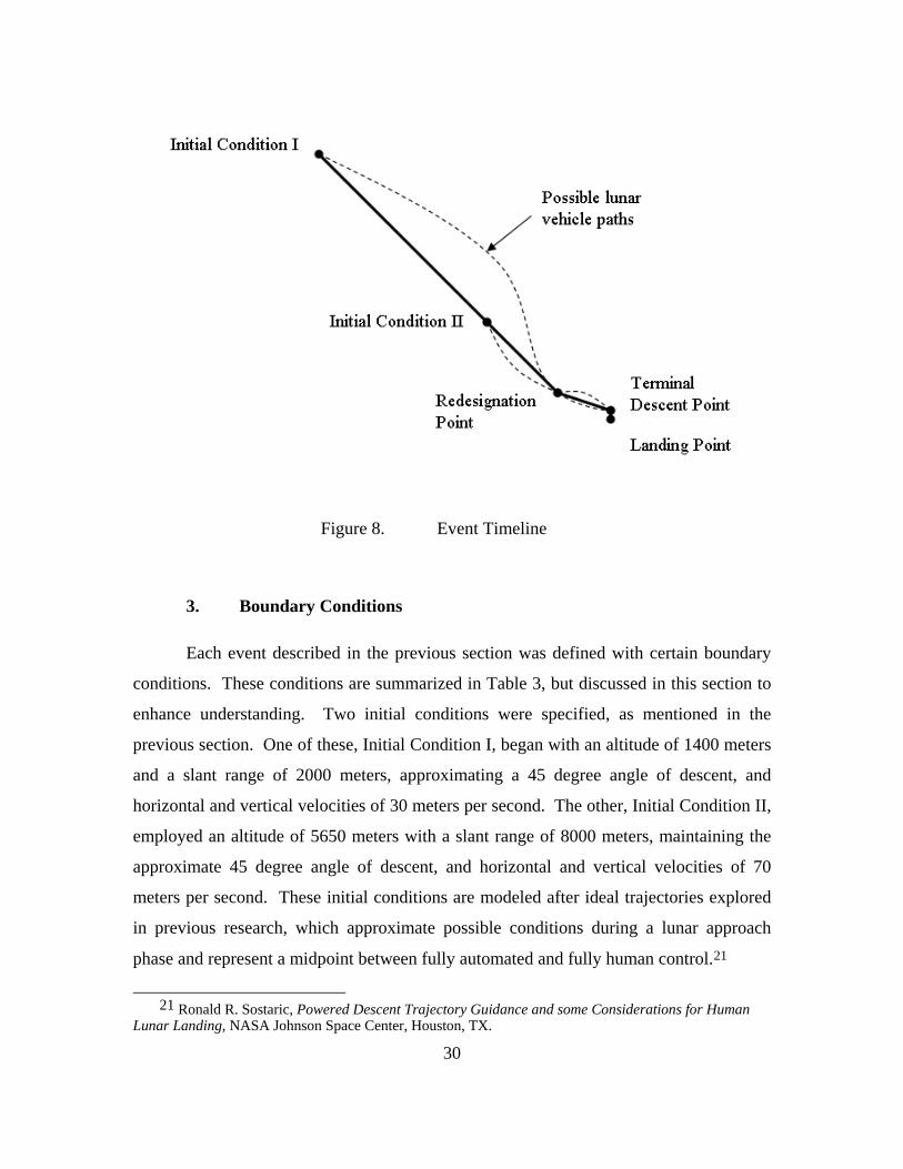
Figure 8. Event Timeline

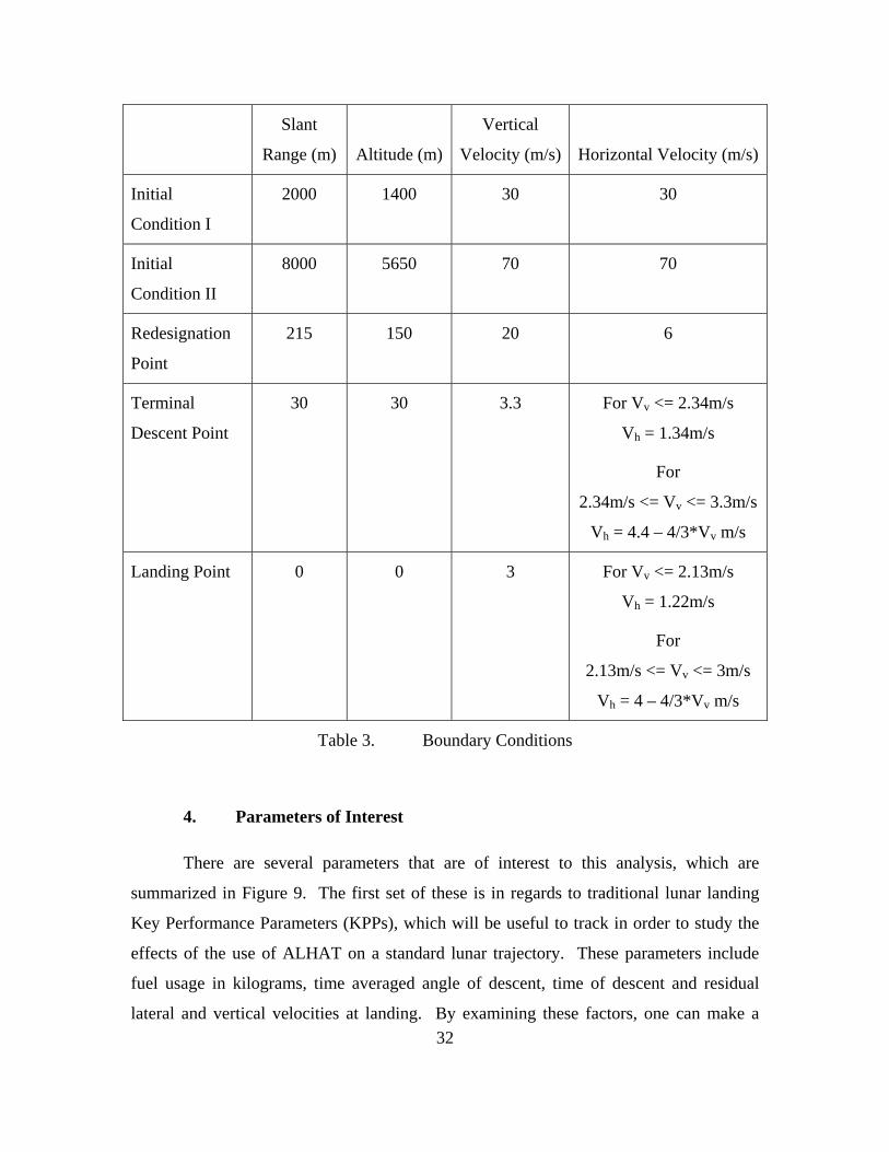
3. Boundary Conditions

Each event described in the previous section was defined with certain boundary

conditions. These conditions are summarized in Table 3, but discussed in this section to

enhance understanding. Two initial conditions were specified, as mentioned in the

previous section. One of these, Initial Condition I, began with an altitude of 1400 meters

and a slant range of 2000 meters, approximating a 45 degree angle of descent, and

horizontal and vertical velocities of 30 meters per second. The other, Initial Condition II,

employed an altitude of 5650 meters with a slant range of 8000 meters, maintaining the

approximate 45 degree angle of descent, and horizontal and vertical velocities of 70

meters per second. These initial conditions are modeled after ideal trajectories explored

in previous research, which approximate possible conditions during a lunar approach

phase and represent a midpoint between fully automated and fully human control.21

30



31

The redesignation point occurs much closer to the landing site, after the HDA

scan has had time to run and a decision to redesignate has been made by some interaction

of the ALHAT system and the human controller. The conditions for this point were

chosen to approximate the last possible opportunity when a redesignation was possible

and include an altitude of 150 meters with a slant range of about 260 meters, enforcing a

redesignated landing point down range of the initial site and a vertical velocities of 20

meters per second and horizontal velocity of 6 meters per second.22

The terminal descent point and the landing point are extremely similar in terms of

constraints. Ideally, the lunar vehicle would have zero horizontal velocity when it

reached the terminal descent point and maintain a constant vertical descent rate until

touchdown. This would indicate that the requirements for each point would be identical.

In practice, however, this correlation is unlikely due to transients remaining from the

approach. As such, it was assumed a 10% margin of error applied to the Apollo Lunar

Module landing constraints was reasonable to derive terminal descent conditions that

accounted for these transients.23 These constraints are somewhat more complex, and are

most easily understood by referring to Table 3 below.



23 Steve Paschall et al., A Self Contained Method for Safe & Precise Lunar Landing, Charles Stark Draper Laboratory, Cambridge, MA, 2008.

32

Slant

Range (m) Altitude (m)

Vertical

Velocity (m/s) Horizontal Velocity (m/s)

Initial

Condition I

2000 1400 30 30

Initial

Condition II

8000 5650 70 70

Redesignation

Point

215 150 20 6

Terminal

Descent Point

30 30 3.3 For Vv <= 2.34m/s

Vh = 1.34m/s

For

2.34m/s <= Vv <= 3.3m/s

Vh = 4.4 – 4/3*Vv m/s

Landing Point 0 0 3 For Vv <= 2.13m/s

Vh = 1.22m/s

For

2.13m/s <= Vv <= 3m/s

Vh = 4 – 4/3*Vv m/s

Table 3. Boundary Conditions

4. Parameters of Interest

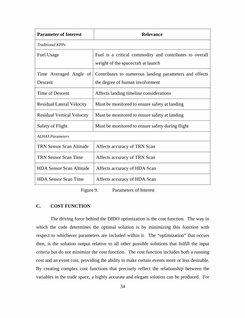
There are several parameters that are of interest to this analysis, which are

summarized in Figure 9. The first set of these is in regards to traditional lunar landing

Key Performance Parameters (KPPs), which will be useful to track in order to study the

effects of the use of ALHAT on a standard lunar trajectory. These parameters include

fuel usage in kilograms, time averaged angle of descent, time of descent and residual

lateral and vertical velocities at landing. By examining these factors, one can make a

33

comparison to the optimal trajectory that does not include the use of ALHAT. In

addition, one can provide a metric for the optimized trajectory using recognizable

parameters.

Along with these general KPPs, additional parameters were considered with

respect to ALHAT. Several open trades exist in the development of ALHAT, and by

monitoring these parameters, guidance can be provided to support progress in certain

areas over others. In addition, requirements and ConOps can be formed by studying

exactly how these parameters vary with the use of different cost functions, as well as their

sensitivities to changes in other parameters. ALHAT related parameters include TRN

sensor scan time, TRN sensor scan altitude, HDA sensor scan time and HDA sensor scan

altitude. Time averaged angle of descent is also important to current ALHAT

development as it relates to human interaction versus HDA sensor reliance.

34

Parameter of Interest Relevance

Traditional KPPs

Fuel Usage Fuel is a critical commodity and contributes to overall

weight of the spacecraft at launch

Time Averaged Angle of

Descent

Contributes to numerous landing parameters and effects

the degree of human involvement

Time of Descent Affects landing timeline considerations

Residual Lateral Velocity Must be monitored to ensure safety at landing

Residual Vertical Velocity Must be monitored to ensure safety at landing

Safety of Flight Must be monitored to ensure safety during flight

ALHAT Parameters

TRN Sensor Scan Altitude Affects accuracy of TRN Scan

TRN Sensor Scan Time Affects accuracy of TRN Scan

HDA Sensor Scan Altitude Affects accuracy of HDA Scan

HDA Sensor Scan Time Affects accuracy of HDA Scan

Figure 9. Parameters of Interest

C. COST FUNCTION

The driving force behind the DIDO optimization is the cost function. The way in

which the code determines the optimal solution is by minimizing this function with

respect to whichever parameters are included within it. The “optimization” that occurs

then, is the solution output relative to all other possible solutions that fulfill the input

criteria but do not minimize the cost function. The cost function includes both a running

cost and an event cost, providing the ability to make certain events more or less desirable.

By creating complex cost functions that precisely reflect the relationship between the

variables in the trade space, a highly accurate and elegant solution can be produced. For

35

the purposes of this study, however, the cost function was kept fairly simple, as the

immaturity of the technology makes it difficult to accurately define. This was done with

an understanding that an improperly formed cost function is far more detrimental to the

optimization of a solution than an overly simplified one.

The resulting cost function for the current study simply provides for the most fuel

efficient trajectory possible. This is done by minimizing the thrust expenditure as one of

the controls. In addition to the optimization on this parameter, other parameters will be

studied to determine any possible trends. By defining the performance of these

parameters and then evaluating whether this performance is sufficient, the relationship

between them becomes more clear, and thereby supports the definition of a more

complex, but still highly accurate, cost function in the future.

D. DIDO OPTIMIZATION

The DIDO optimization code requires the development of five different files in

order to accurately specify the problem. Once the problem is defined, DIDO optimizes a

solution using the restrictions found in the problem definition and with respect to the cost

function as previously discussed. These files include the Cost Function File, Dynamics

Function File, Events File, Path File and Problem File. The first four of these files were

created in Matlab as independent functions, called by the parent Problem File. In order to

understand how the ALHAT system was modeled by the DIDO optimization program, it

is necessary to examine each of these files in turn. A summary of each file rather than

the full code is presented in the text for simplification purposes, however, all files are

available as appendices to this document if further study is desired.

1. Cost Function File

The Cost Function File (Appendix A) is perhaps the most important portion of the

file code as it allows DIDO to solve for a system optimization. The essence of the DIDO

code is the minimization of this cost function, which represents an optimized solution. In

the case of this study, the decision was made to keep the cost function relatively simple,

favoring post optimization analysis to determine the benefit of the results, rather than an

36

initial attempt at forming an equation that accurately defines relationships between

currently ill defined variables. This method was discussed previously and will not be

expanded on here. What is important to note is that this file is where the specifics of the

optimization are defined. Changing this function file will result in a new solution for the

system optimization, so it is crucial that this function accurately represents the

importance of the parameters of interest.

2. Dynamics Function File

The Dynamics Function File specifies the vertical (Appendix B) and horizontal

(Appendix C) equations of motion with regard to the lunar vehicle. These are simple

differential equations of motion in the horizontal and vertical planes. The decision was

made not to include a third spatial dimension with respect to lunar vehicle motion, as this

would add significant complexity without much overall benefit to the analysis. This

could be a region of improvement for later study; however, for the purposes of evaluating

basic ALHAT parameters, it is largely irrelevant in which lateral direction motion occurs,

it is only important to distinguish between vertical and horizontal motion. For an in

depth analysis of total fuel consumption, this would be an important feature to include

due to variations in out of plane maneuvers, however, the current analysis is more

interested in the difference in fuel consumption from one trajectory to another rather than

overall usage. In addition to the equations of motion, their derivatives are also defined in

this function, such that the optimization can properly account for the variables over the

duration of the event timeline.

3. Events Function File

The Events Function File (Appendix D) is used to designate boundary conditions

of the simulated lunar landing. This file dictates the necessary initial and final conditions

of all state variables as defined in the Dynamics Function File, in this case altitude,

velocity and mass. It is important to keep in mind that although these parameters are

defined in this file, they are not necessarily set as fixed values. The initial boundary

condition is defined with typical values reflecting the lunar approach phase, as described

37

previously. The final conditions, however, are left largely undefined, so that the final

fuel mass and velocity may vary. It is not necessary within the simulation to completely

deplete the available fuel, and it is not necessary to have a zero velocity upon landing, as

long as the velocity is less than the defined minimum value to avoid damaging the

landing vehicle. In addition to the initial and final boundary conditions, this file could be

used to define the redesignation point and terminal descent conditions, however, in an

effort to consider the redesignation a decision made in real time, rather than a forgone

conclusion, these events were considered separately from the initial trajectory.

4. Path Function File

The Path Function File imposes certain restrictions on the path the landing vehicle

must take. For an open ended problem, there would be no path restriction. For an

extremely in depth analysis of the ALHAT control system, a path restriction function

could be made with respect to a randomly generated terrain, where the hazards created

limits to landing areas and thus alter the optimal path. For the purposes of this analysis,

however, the path is left to vary as the optimization allows. The only restrictions to the

actual trajectory the LSAM follows are defined with regards to its initial and final

boundary conditions, as previously discussed, and an upper and lower limit on altitude as

will be defined in the Problem Function File. This simple path does not require any

additional definition within the Path Function File, and so none was used. The previous

efforts to establish a reasonable path enforce the use of the ALHAT system’s capabilities

on the lunar trajectory in order to study the resulting effects on the desired parameters of

interest without additional constraint.

5. Problem File

The Problem File designates the constants used with respect to a lunar

environment and the proposed LSAM, as well as the bounds in which the variables are

able to range. Most of these parameters are open to vary across large ranges, however,

some, like mass and thrust, have physical limitations that must be sustained. The

constants, such as the lunar gravitational constant and the estimated LSAM mass, as well

38

as the variables, such as available thrust, could also be revised in future analysis as

LSAM specifications are further refined. In addition to defining constants and ranges,

the Problem File is used to call the various Function Files, and to specifically set the

initial condition values. As such, a separate Problem File was created and recorded in the

appendices for the Initial Condition I (Appendix E) and Initial Condition II (Appendix F)

trajectories.

E. CHAPTER SUMMARY

In order to create an accurate and effective model, three major components were

considered: the lunar vehicle, the lunar environment and the parameters of interest. By

modeling the environment after what was experienced during the Apollo missions, the

model has been anchored with actual data. By using best estimates of the LSAM design

and simplifying its application, the model accounts for the possibility of change as the

components continue to develop and mature. And by selecting specific parameters of

interest, the model ensures its usefulness in both the determination of the optimal

trajectory with respect to the cost function via a DIDO optimization, as well as the

examination of effects of the ALHAT system on this trajectory; applications which

directly reflect the objectives of the thesis as defined in Chapter I.

39

V. RESEARCH ANALYSIS

A. INTRODUCTION

The analysis performed with respect to this research followed as closely as

possible to the initial objectives and paths that have thus far been laid out. In the course

of study, however, certain unforeseen constraints arose and were accounted for. These

constraints are characterized, in order to qualify the results that follow. The results have

all been generated using DIDO as well as the Matlab scripts discussed in the previous

chapter, and attached as appendices. All plots are generated by the script included as

Appendix G. In addition to the physical trajectories which were created using the DIDO

optimization, several parameters of interest were studied to better characterize the results.

B. CONSTRAINTS

Although the best efforts were made to create a suitably realistic simulation, there

were certain limitations that were not overcome in the course of this research. Several of

the DIDO constraints are artifacts of the version of code that was employed. A

professional version of DIDO is available that would greatly alleviate these issues, but

obtaining a copy of this was outside the budget of the current research. In addition,

because the ALHAT system is still in development, certain constraints were levied due to

the uncertainty of its final design. It is possible that these limitations can be resolved or

worked around in future analysis, but they are stated here in order to qualify the results.

1. DIDO

Utilization of DIDO as an optimization method was extremely beneficial to the

analysis of this problem. However, there were a few limitations that the code imposed.

As stated previously, most of these limitations could be avoided via implementation of

the professional DIDO code; this was simply outside the scope of the current research.

40

a. State Variables

The main complication caused by the rudimentary version of DIDO used

was that it limited the number of state variables that could be analyzed at once. As a

result, the analysis had to be performed in separate planes, examining the horizontal and

vertical planes individually, and then combining the results. Hence, thrust and motion

occurred in only one plane. To ensure that the analysis remained consistent and valid,

each event was performed individually, any discrepancies or differences in boundary

conditions were examined, and the events were reanalyzed using refined parameters until

a single, consistent solution was achieved. In particular, it was found that the horizontal

motion of the vehicle took significantly more time than the vertical motion. To combine

these, the horizontal motion was left unconstrained with respect to time, and the vertical

motion was then solved with a fixed final time equal to that of the resultant horizontal

motion. This difficulty and additional manual scrutiny reduces the precision of the

analysis, but not the utility. Because this research is meant to be a starting point for

consideration of both DIDO utilization and ALHAT capabilities, rather than an in depth

examination of the precise values of the results, it maintains a great deal of usefulness.

This initial constraint is the source of the remaining constraints, which will be discussed

in turn, along with the steps taken to minimize their impact.

b. Mass

The separation of vertical and horizontal planes impacted those variables

that were dependent on each, such as mass. The overall mass of the spacecraft is

decreasing as thrusters are fired in both planes; as such, this effect should be taken into

account continuously in order to ensure the force required to navigate the vehicle is

correct. However, as the primary thrust was seen to be in the vertical direction, the

effects of segregating the two were greatly reduced. In the vertical plane, the reduction in

mass was nearly exact due to the relatively small amount spent in the horizontal plane,

and conversely, the error induced in the horizontal plane was extremely small relative to

the total. In addition, at the boundary of each event analyzed in the timeline, the

contributions of each plane were summed, and the initial mass of the new event was set

41

equal for both. The result is a degree of inaccuracy in the mass calculation, but given the

status of the mass budget as a currently open trade anyway, the usefulness of this research

with respect to the trend of the mass usage remains sound.

c. Nodes

In addition to the limit of the number of state variables used in the

analysis, the number of nodes was constrained as well. The nodes are used to separate

the optimization calculation into a number of discrete points. These points are not equal

in time, as DIDO does not propagate variables through time, but can still be thought of as

endpoints for pieces of the optimization, which, when combined, create the overall

trajectory. The more pieces, or nodes, used to determine the optimization, the more

accurate the result. Although the maximum number of nodes allowed in the version of

DIDO which was implemented was used, it seemed that a greater number would smooth

some of the results. In particular, nodes that separated larger periods of time tended to

induce more error in the results and expectedly smooth or constant results, such as fuel

usage, had more variation than predicted. Again, this constraint does not limit the

intended trend benefits of the analysis, but rather the finite precision.

2. ALHAT

One of the objectives of this research was to identify changes in the ideal

trajectory resulting from hazard avoidance. Because of this, some parameters in the

analysis were optimized for ALHAT by default. In particular, the angle of attack of the

spacecraft was chosen to be zero degrees throughout the flight, or exactly as the vehicle

would stand on the ground. This choice was motivated both by the increased accuracy

and effectiveness of the ALHAT sensors, as well as for the simplification in separating

the vertical and horizontal thrust control parameters in the DIDO optimization, as

previously discussed. In effect, this type of analysis demonstrates the possibility of using

a largely automatic control, rather than manual input, a trade which is still ongoing. The

effect of this implementation is that the horizontal motion of the LSAM takes longer, due

to the reduced thrust available in that direction. As such, the vertical thrust is tasked with

42

staying aloft in addition to simply braking. This particular constraint necessitates a flight

configuration that is rather unlikely to remain the final method for lunar landing, but it is

the intention of this analysis to put forth an initial starting point of optimized autonomous

ALHAT control, which can be expanded and revised through additional research.

C. TRAJECTORY RESULTS

The lunar landing trajectory was broken into different events, as described

previously. These events will be presented individually for distinct analysis, then as a

whole for overall understanding. This trajectory is the DIDO optimized result of the

LSAM incorporating ALHAT system technology with respect to the previously stated

constraints. In particular, this trajectory is that of a fixed vertical orientation LSAM, with

time unconstrained horizontal motion and time fixed vertical motion tied to specific

velocity and position boundary conditions, optimized for minimum fuel consumption.

Additional in depth evaluation of this optimization as well as individual parameters will

be provided later.

1. Initial Condition I

Initial Condition I represents a 2,000 kilometer slant angle trajectory with an

initial expected landing point about 1400 meters downrange and boundary conditions as

dictated in Table 3. The physical path of the trajectory is shown in Figure 10. It can be

seen that the optimized path calls for a descent in the vertical direction, followed by a

burn and another descent. As previously discussed in the constraints, the horizontal

motion requires more time to complete than the vertical motion, due to the limited

horizontal thrust resulting from the zero degree angle of attack, and so this burn is

necessary to keep the LSAM aloft while it travels sufficiently far down range. Although

alternative trajectories such as maintaining a constant altitude, followed by a single

descent, or a constant gradual descent are viable solutions, the path solved for by DIDO

and depicted below is the most efficient in terms of fuel consumption, and thus is the

“optimal” solution in terms of this analysis. Despite this efficiency, the large fall and rise

may indicate a need for additional parameters to be considered and included within the

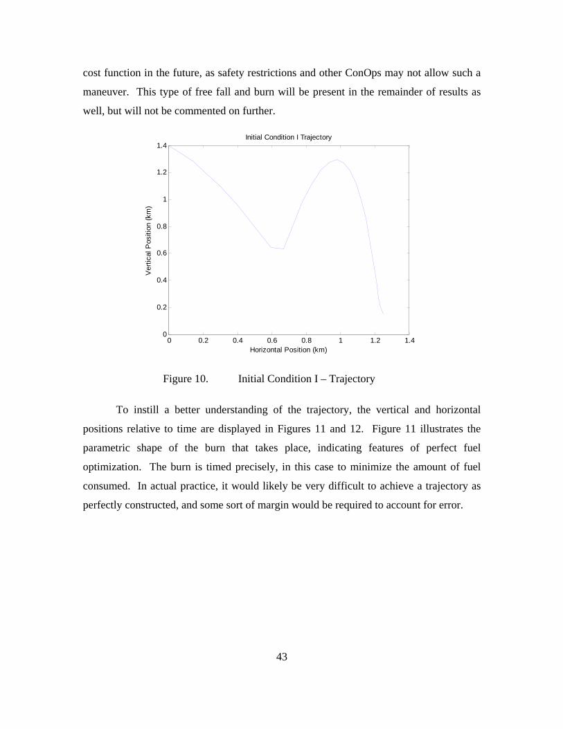
cost function in the future, as safety restrictions and other ConOps may not allow such a

maneuver. This type of free fall and burn will be present in the remainder of results as

well, but will not be commented on further.

0 0.2 0.4 0.6 0.8 1 1.2 1.40

0.2

0.4

0.6

0.8

1

1.2

1.4Initial Condition I Trajectory

Horizontal Position (km)

Ver

tical

Pos

ition

(km

)

Figure 10. Initial Condition I – Trajectory

To instill a better understanding of the trajectory, the vertical and horizontal

positions relative to time are displayed in Figures 11 and 12. Figure 11 illustrates the

parametric shape of the burn that takes place, indicating features of perfect fuel

optimization. The burn is timed precisely, in this case to minimize the amount of fuel

consumed. In actual practice, it would likely be very difficult to achieve a trajectory as

perfectly constructed, and some sort of margin would be required to account for error.

43

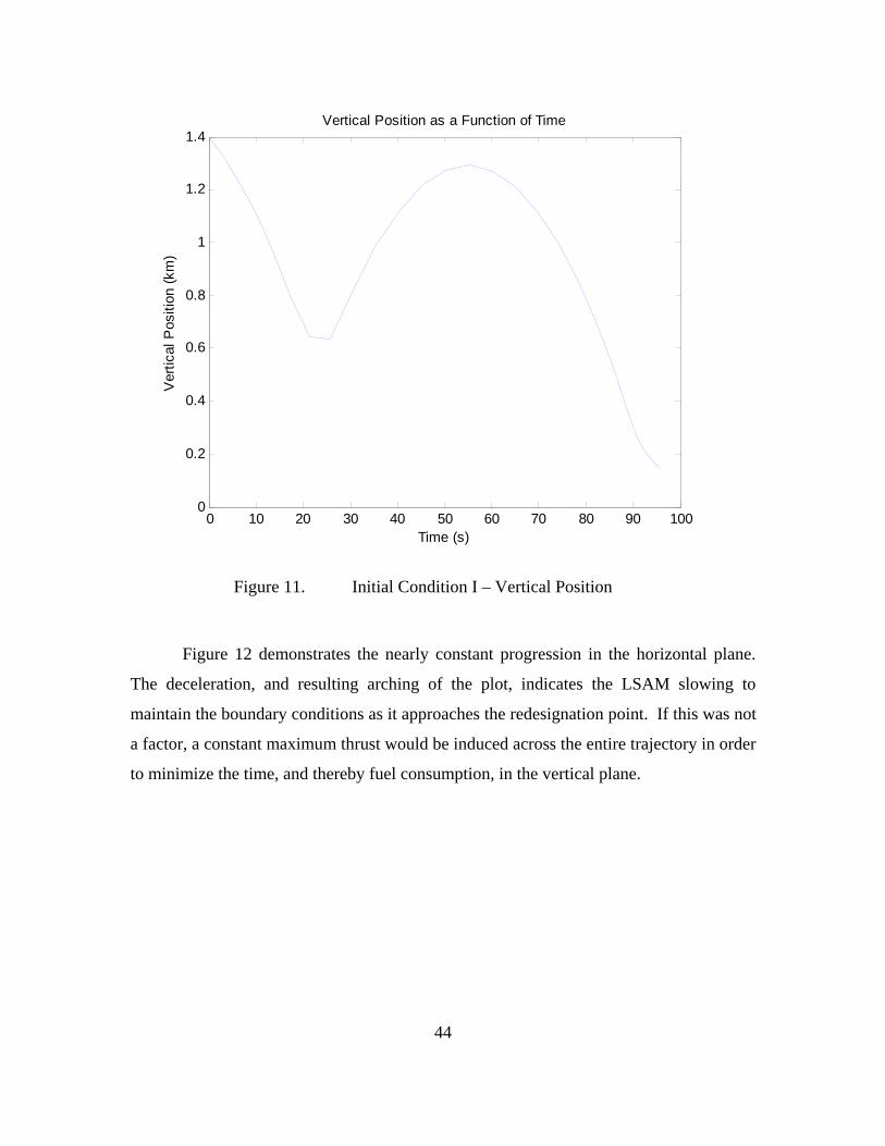
0 10 20 30 40 50 60 70 80 90 1000

0.2

0.4

0.6

0.8

1

1.2

1.4Vertical Position as a Function of Time

Time (s)

Ver

tical

Pos

ition

(km

)

Figure 11. Initial Condition I – Vertical Position

Figure 12 demonstrates the nearly constant progression in the horizontal plane.

The deceleration, and resulting arching of the plot, indicates the LSAM slowing to

maintain the boundary conditions as it approaches the redesignation point. If this was not

a factor, a constant maximum thrust would be induced across the entire trajectory in order

to minimize the time, and thereby fuel consumption, in the vertical plane.

44

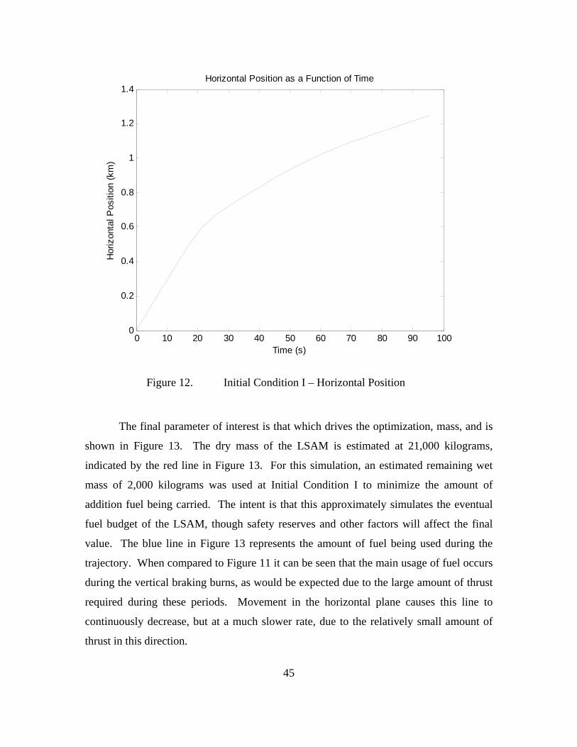
0 10 20 30 40 50 60 70 80 90 1000

0.2

0.4

0.6

0.8

1

1.2

1.4Horizontal Position as a Function of Time

Time (s)

Hor

izon

tal P

ositi

on (

km)

Figure 12. Initial Condition I – Horizontal Position

The final parameter of interest is that which drives the optimization, mass, and is

shown in Figure 13. The dry mass of the LSAM is estimated at 21,000 kilograms,

indicated by the red line in Figure 13. For this simulation, an estimated remaining wet

mass of 2,000 kilograms was used at Initial Condition I to minimize the amount of

addition fuel being carried. The intent is that this approximately simulates the eventual

fuel budget of the LSAM, though safety reserves and other factors will affect the final

value. The blue line in Figure 13 represents the amount of fuel being used during the

trajectory. When compared to Figure 11 it can be seen that the main usage of fuel occurs

during the vertical braking burns, as would be expected due to the large amount of thrust

required during these periods. Movement in the horizontal plane causes this line to

continuously decrease, but at a much slower rate, due to the relatively small amount of

thrust in this direction.

45

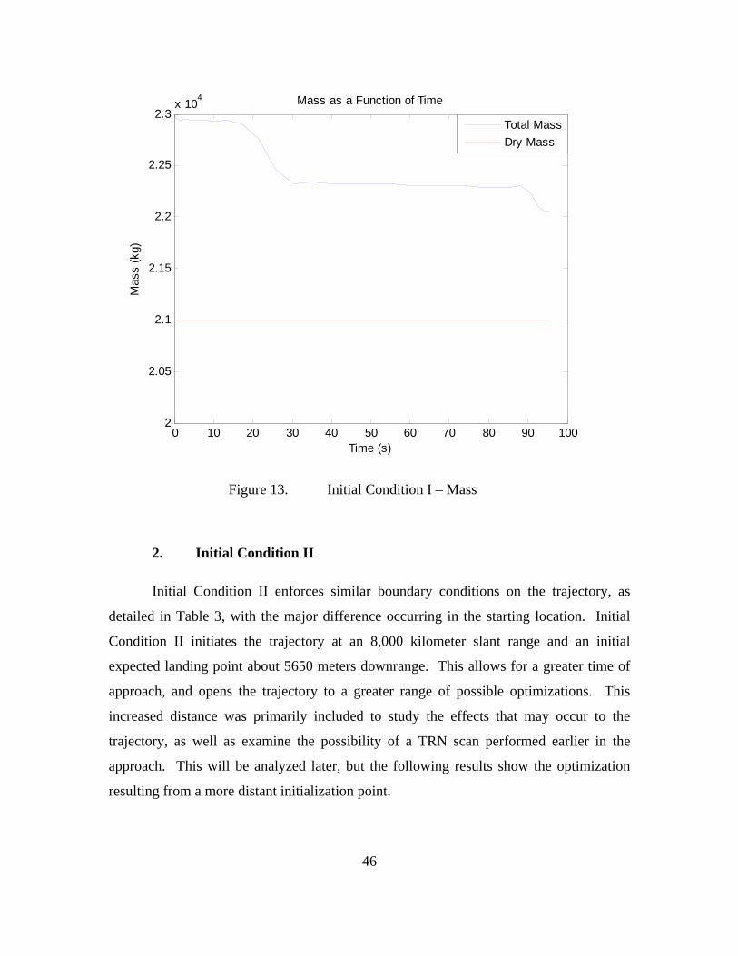
0 10 20 30 40 50 60 70 80 90 1002

2.05

2.1

2.15

2.2

2.25

2.3x 10

4 Mass as a Function of Time

Time (s)

Mas

s (k

g)Total Mass

Dry Mass

Figure 13. Initial Condition I – Mass

2. Initial Condition II

Initial Condition II enforces similar boundary conditions on the trajectory, as

detailed in Table 3, with the major difference occurring in the starting location. Initial

Condition II initiates the trajectory at an 8,000 kilometer slant range and an initial

expected landing point about 5650 meters downrange. This allows for a greater time of

approach, and opens the trajectory to a greater range of possible optimizations. This

increased distance was primarily included to study the effects that may occur to the

trajectory, as well as examine the possibility of a TRN scan performed earlier in the

approach. This will be analyzed later, but the following results show the optimization

resulting from a more distant initialization point.

46

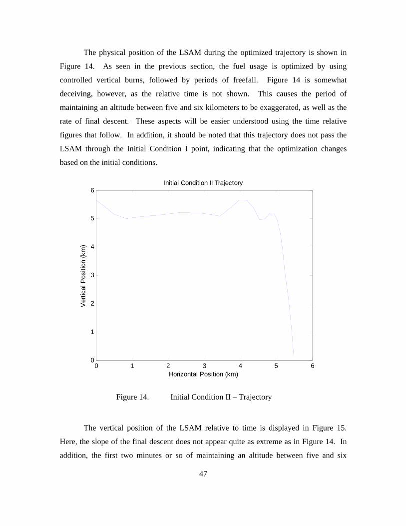
The physical position of the LSAM during the optimized trajectory is shown in

Figure 14. As seen in the previous section, the fuel usage is optimized by using

controlled vertical burns, followed by periods of freefall. Figure 14 is somewhat

deceiving, however, as the relative time is not shown. This causes the period of

maintaining an altitude between five and six kilometers to be exaggerated, as well as the

rate of final descent. These aspects will be easier understood using the time relative

figures that follow. In addition, it should be noted that this trajectory does not pass the

LSAM through the Initial Condition I point, indicating that the optimization changes

based on the initial conditions.

0 1 2 3 4 5 60

1

2

3

4

5

6Initial Condition II Trajectory


Ver

tical

Pos

ition

(km

)

Figure 14. Initial Condition II – Trajectory

The vertical position of the LSAM relative to time is displayed in Figure 15.

Here, the slope of the final descent does not appear quite as extreme as in Figure 14. In

addition, the first two minutes or so of maintaining an altitude between five and six

47

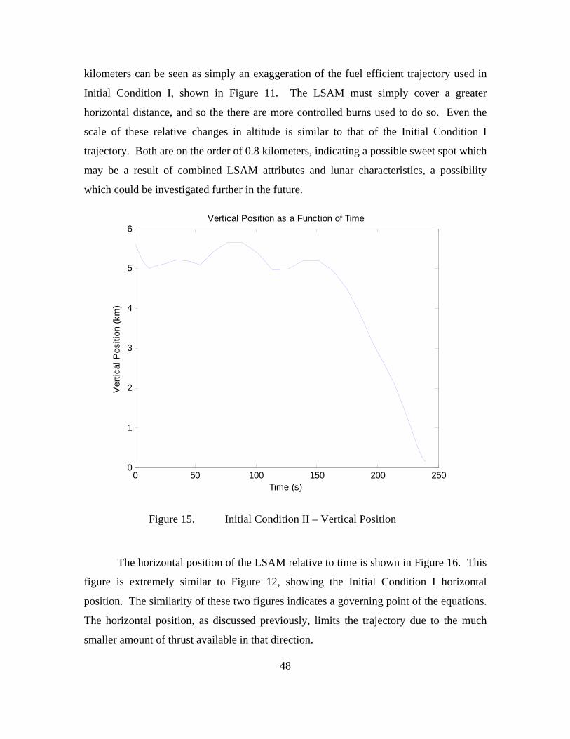
kilometers can be seen as simply an exaggeration of the fuel efficient trajectory used in

Initial Condition I, shown in Figure 11. The LSAM must simply cover a greater

horizontal distance, and so the there are more controlled burns used to do so. Even the

scale of these relative changes in altitude is similar to that of the Initial Condition I

trajectory. Both are on the order of 0.8 kilometers, indicating a possible sweet spot which

may be a result of combined LSAM attributes and lunar characteristics, a possibility

which could be investigated further in the future.

0 50 100 150 200 2500

1

2

3

4

5

6Vertical Position as a Function of Time

Time (s)

Ver

tical

Pos

ition

(km

)

Figure 15. Initial Condition II – Vertical Position

The horizontal position of the LSAM relative to time is shown in Figure 16. This

figure is extremely similar to Figure 12, showing the Initial Condition I horizontal

position. The similarity of these two figures indicates a governing point of the equations.

The horizontal position, as discussed previously, limits the trajectory due to the much

smaller amount of thrust available in that direction.

48

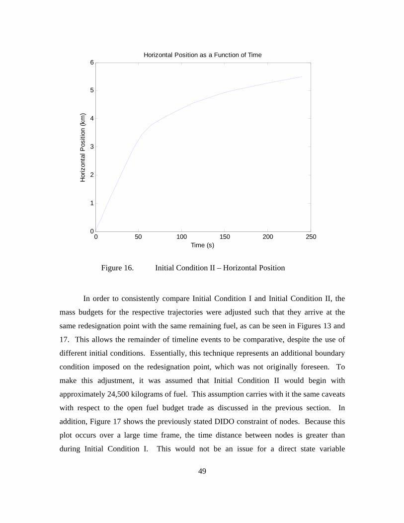
0 50 100 150 200 2500

1

2

3

4

5

6Horizontal Position as a Function of Time

Time (s)

Hor

izon

tal P

ositi

on (

km)

Figure 16. Initial Condition II – Horizontal Position

In order to consistently compare Initial Condition I and Initial Condition II, the

mass budgets for the respective trajectories were adjusted such that they arrive at the

same redesignation point with the same remaining fuel, as can be seen in Figures 13 and

17. This allows the remainder of timeline events to be comparative, despite the use of

different initial conditions. Essentially, this technique represents an additional boundary

condition imposed on the redesignation point, which was not originally foreseen. To

make this adjustment, it was assumed that Initial Condition II would begin with

approximately 24,500 kilograms of fuel. This assumption carries with it the same caveats

with respect to the open fuel budget trade as discussed in the previous section. In

addition, Figure 17 shows the previously stated DIDO constraint of nodes. Because this

plot occurs over a large time frame, the time distance between nodes is greater than

during Initial Condition I. This would not be an issue for a direct state variable

49

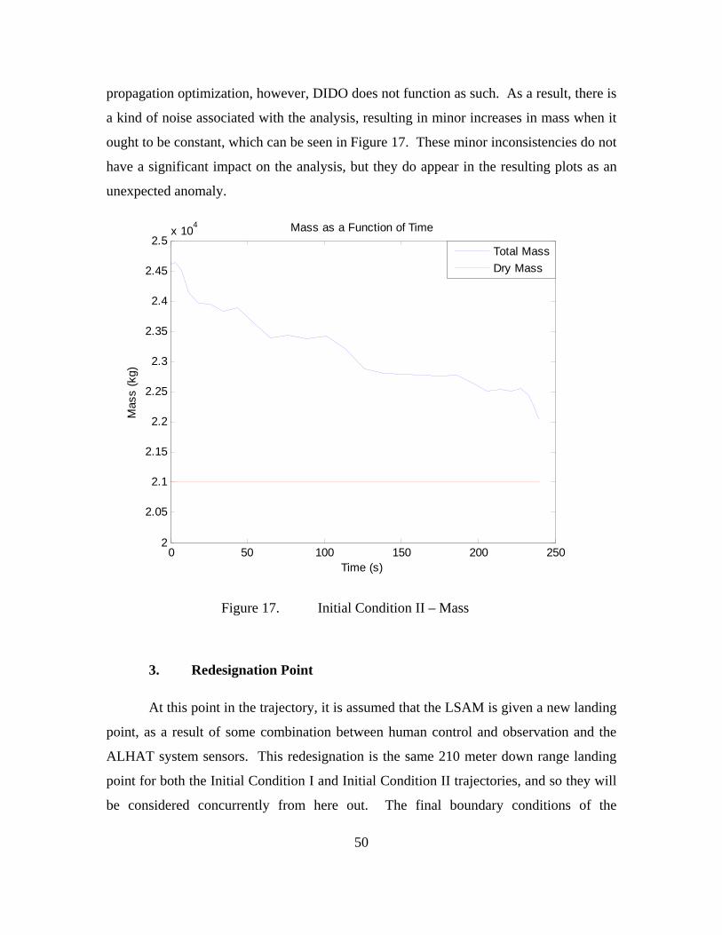
propagation optimization, however, DIDO does not function as such. As a result, there is

a kind of noise associated with the analysis, resulting in minor increases in mass when it

ought to be constant, which can be seen in Figure 17. These minor inconsistencies do not

have a significant impact on the analysis, but they do appear in the resulting plots as an

unexpected anomaly.

0 50 100 150 200 2502

2.05

2.1

2.15

2.2

2.25

2.3

2.35

2.4

2.45

2.5x 10


Time (s)

Mas

s (k

g)

Total Mass

Dry Mass

Figure 17. Initial Condition II – Mass

3. Redesignation Point

At this point in the trajectory, it is assumed that the LSAM is given a new landing

point, as a result of some combination between human control and observation and the

ALHAT system sensors. This redesignation is the same 210 meter down range landing

point for both the Initial Condition I and Initial Condition II trajectories, and so they will

be considered concurrently from here out. The final boundary conditions of the

50

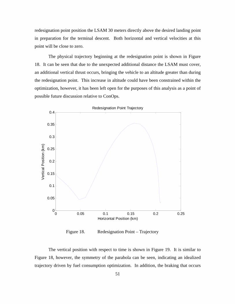
redesignation point position the LSAM 30 meters directly above the desired landing point

in preparation for the terminal descent. Both horizontal and vertical velocities at this

point will be close to zero.

The physical trajectory beginning at the redesignation point is shown in Figure

18. It can be seen that due to the unexpected additional distance the LSAM must cover,

an additional vertical thrust occurs, bringing the vehicle to an altitude greater than during

the redesignation point. This increase in altitude could have been constrained within the

optimization, however, it has been left open for the purposes of this analysis as a point of

possible future discussion relative to ConOps.

0 0.05 0.1 0.15 0.2 0.250

0.05

0.1

0.15

0.2

0.25

0.3

0.35

0.4Redesignation Point Trajectory


Ver

tical

Pos

ition

(km

)

Figure 18. Redesignation Point – Trajectory

The vertical position with respect to time is shown in Figure 19. It is similar to

Figure 18, however, the symmetry of the parabola can be seen, indicating an idealized

trajectory driven by fuel consumption optimization. In addition, the braking that occurs

51

at the end of the trajectory is more apparent as the vertical position is largely maintained

as the respective velocities are slowed to achieve the proper boundary conditions.

0 10 20 30 40 50 600

0.05

0.1

0.15

0.2

0.25

0.3

0.35


Time (s)

Ver

tical

Pos

ition

(km

)

Figure 19. Redesignation Point – Vertical Position

The horizontal position relative to time is displayed in Figure 20. As the previous

analyses of the initial conditions have demonstrated, the horizontal position is a limiting

factor in the optimization prior to the redesignation point. As evidenced by Figure 20,

this remains the case after the redesignation point has been reached as well. The

horizontal position increases at the maximum rate in order to minimize the amount of fuel

used to keep the LSAM aloft in the vertical plane. It slows only at the end in order to

achieve the near zero velocity required for Terminal Descent.

52

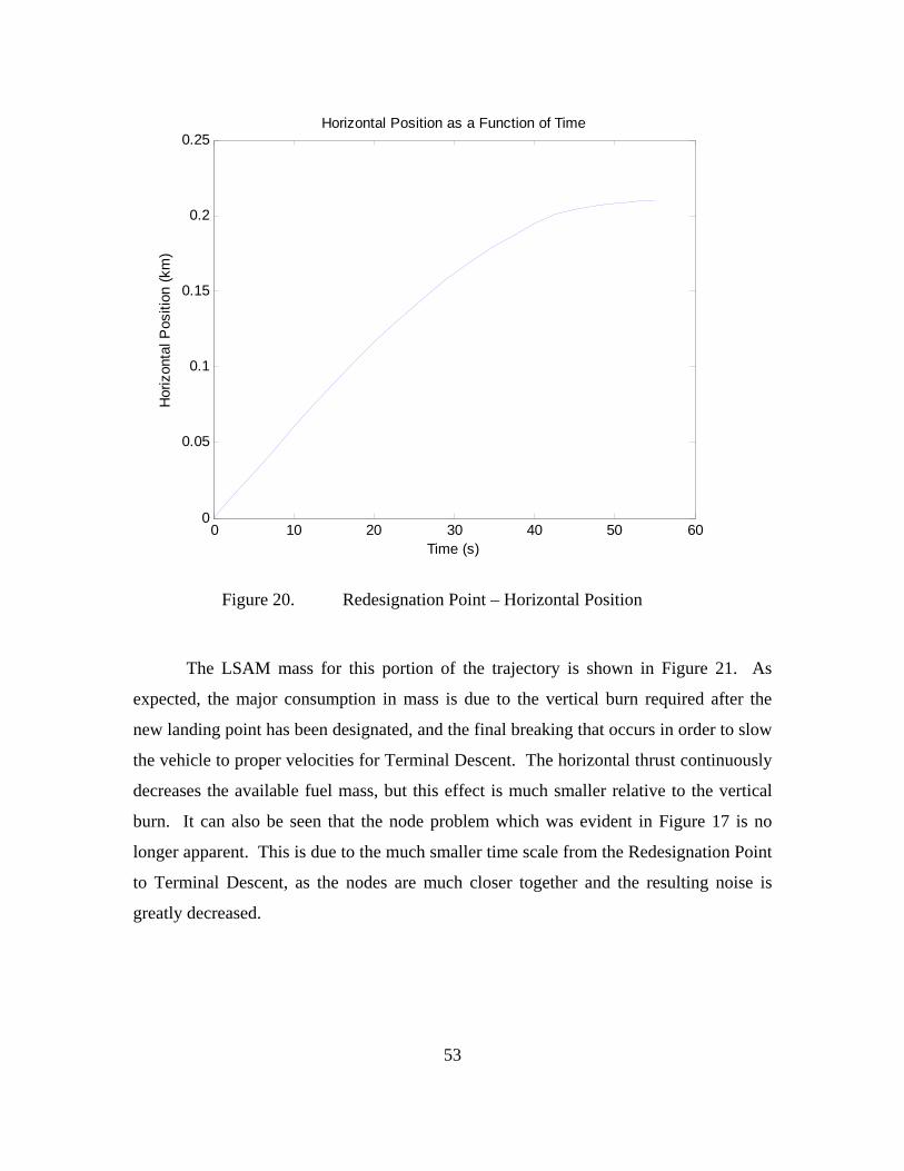
0 10 20 30 40 50 600

0.05

0.1

0.15

0.2

0.25Horizontal Position as a Function of Time

Time (s)

Hor

izon

tal P

ositi

on (

km)

Figure 20. Redesignation Point – Horizontal Position

The LSAM mass for this portion of the trajectory is shown in Figure 21. As

expected, the major consumption in mass is due to the vertical burn required after the

new landing point has been designated, and the final breaking that occurs in order to slow

the vehicle to proper velocities for Terminal Descent. The horizontal thrust continuously

decreases the available fuel mass, but this effect is much smaller relative to the vertical

burn. It can also be seen that the node problem which was evident in Figure 17 is no

longer apparent. This is due to the much smaller time scale from the Redesignation Point

to Terminal Descent, as the nodes are much closer together and the resulting noise is

greatly decreased.

53

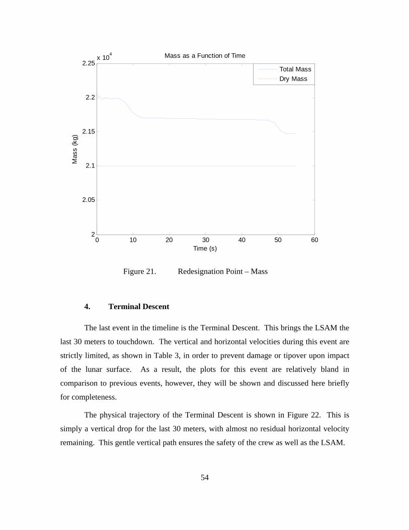
0 10 20 30 40 50 602

2.05

2.1

2.15

2.2

2.25x 10


Time (s)

Mas

s (k

g)Total Mass

Dry Mass

Figure 21. Redesignation Point – Mass

4. Terminal Descent

The last event in the timeline is the Terminal Descent. This brings the LSAM the

last 30 meters to touchdown. The vertical and horizontal velocities during this event are

strictly limited, as shown in Table 3, in order to prevent damage or tipover upon impact

of the lunar surface. As a result, the plots for this event are relatively bland in

comparison to previous events, however, they will be shown and discussed here briefly

for completeness.

The physical trajectory of the Terminal Descent is shown in Figure 22. This is

simply a vertical drop for the last 30 meters, with almost no residual horizontal velocity

remaining. This gentle vertical path ensures the safety of the crew as well as the LSAM.

54

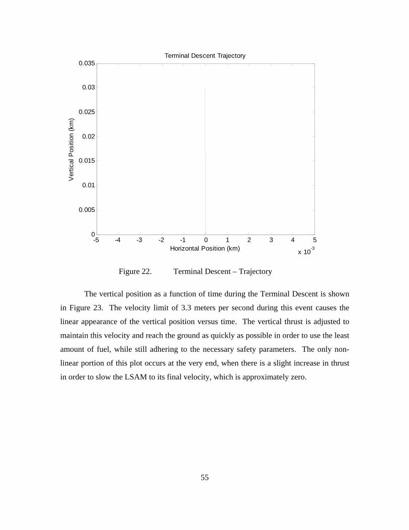
-5 -4 -3 -2 -1 0 1 2 3 4 5

x 10-3

0

0.005

0.01

0.015

0.02

0.025

0.03

0.035Terminal Descent Trajectory


Ver

tical

Pos

ition

(km

)

Figure 22. Terminal Descent – Trajectory

The vertical position as a function of time during the Terminal Descent is shown

in Figure 23. The velocity limit of 3.3 meters per second during this event causes the

linear appearance of the vertical position versus time. The vertical thrust is adjusted to

maintain this velocity and reach the ground as quickly as possible in order to use the least

amount of fuel, while still adhering to the necessary safety parameters. The only non-

linear portion of this plot occurs at the very end, when there is a slight increase in thrust

in order to slow the LSAM to its final velocity, which is approximately zero.

55

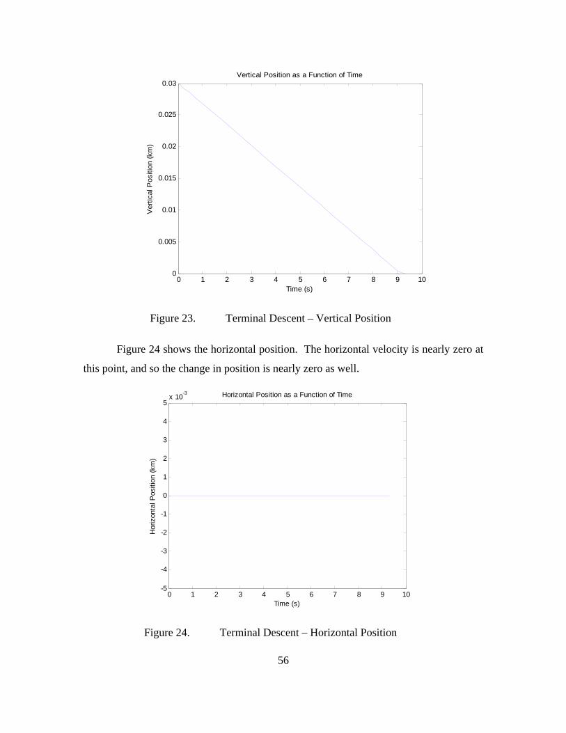
0 1 2 3 4 5 6 7 8 9 100

0.005

0.01

0.015

0.02

0.025


Time (s)

Ver

tical

Pos

ition

(km

)

Figure 23. Terminal Descent – Vertical Position

Figure 24 shows the horizontal position. The horizontal velocity is nearly zero at

this point, and so the change in position is nearly zero as well.

0 1 2 3 4 5 6 7 8 9 10-5

-4

-3

-2

-1

0

1

2

3

4

5x 10

-3 Horizontal Position as a Function of Time

Time (s)

Hor

izon

tal P

ositi

on (

km)

Figure 24. Terminal Descent – Horizontal Position

56

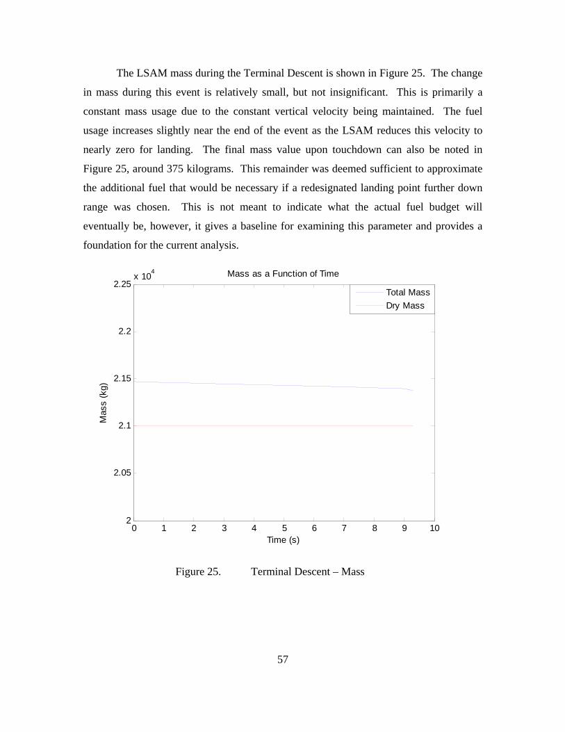
The LSAM mass during the Terminal Descent is shown in Figure 25. The change

in mass during this event is relatively small, but not insignificant. This is primarily a

constant mass usage due to the constant vertical velocity being maintained. The fuel

usage increases slightly near the end of the event as the LSAM reduces this velocity to

nearly zero for landing. The final mass value upon touchdown can also be noted in

Figure 25, around 375 kilograms. This remainder was deemed sufficient to approximate

the additional fuel that would be necessary if a redesignated landing point further down

range was chosen. This is not meant to indicate what the actual fuel budget will

eventually be, however, it gives a baseline for examining this parameter and provides a

foundation for the current analysis.

0 1 2 3 4 5 6 7 8 9 102

2.05

2.1

2.15

2.2

2.25x 10


Time (s)

Mas

s (k

g)

Total Mass

Dry Mass

Figure 25. Terminal Descent – Mass

57

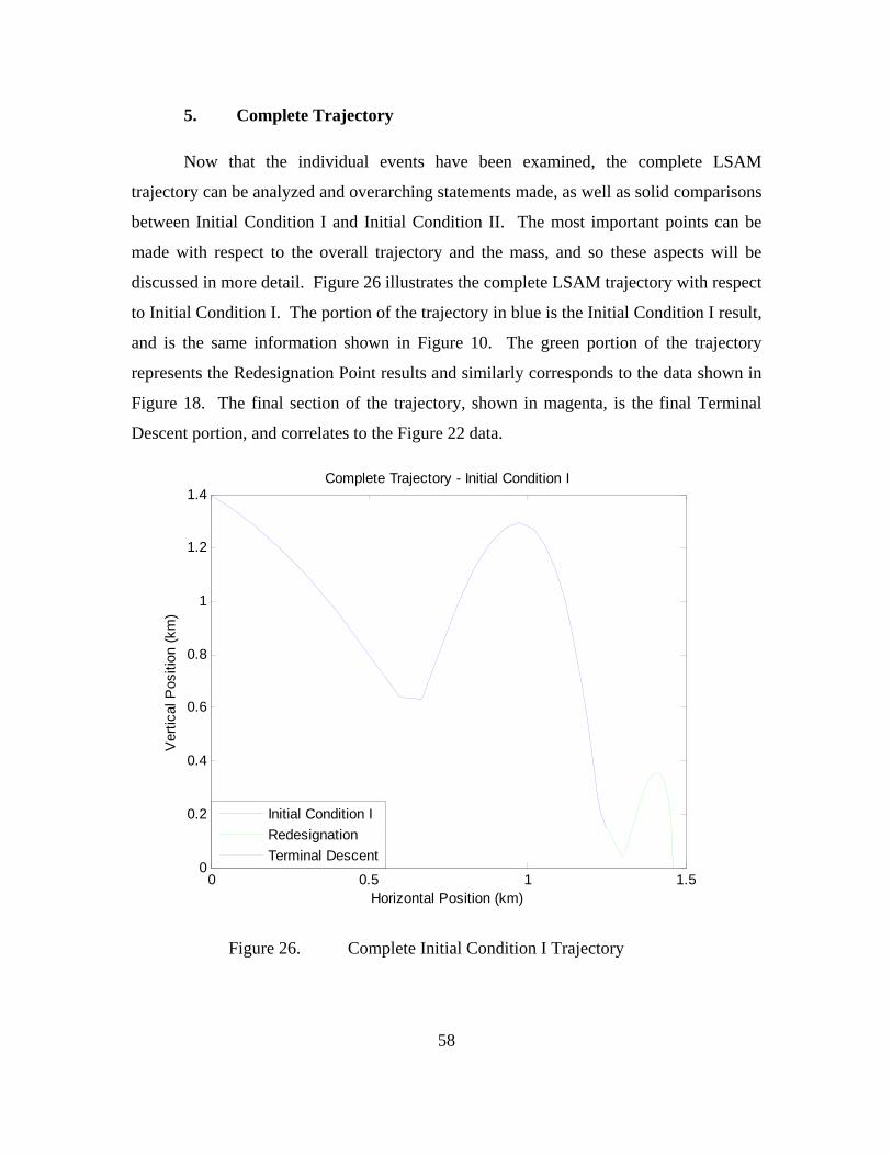
5. Complete Trajectory

Now that the individual events have been examined, the complete LSAM

trajectory can be analyzed and overarching statements made, as well as solid comparisons

between Initial Condition I and Initial Condition II. The most important points can be

made with respect to the overall trajectory and the mass, and so these aspects will be

discussed in more detail. Figure 26 illustrates the complete LSAM trajectory with respect

to Initial Condition I. The portion of the trajectory in blue is the Initial Condition I result,

and is the same information shown in Figure 10. The green portion of the trajectory

represents the Redesignation Point results and similarly corresponds to the data shown in

Figure 18. The final section of the trajectory, shown in magenta, is the final Terminal

Descent portion, and correlates to the Figure 22 data.

0 0.5 1 1.50

0.2

0.4

0.6

0.8

1

1.2

1.4Complete Trajectory - Initial Condition I


Ver

tical

Pos

ition

(km

)

Initial Condition I

Redesignation

Terminal Descent

Figure 26. Complete Initial Condition I Trajectory

58

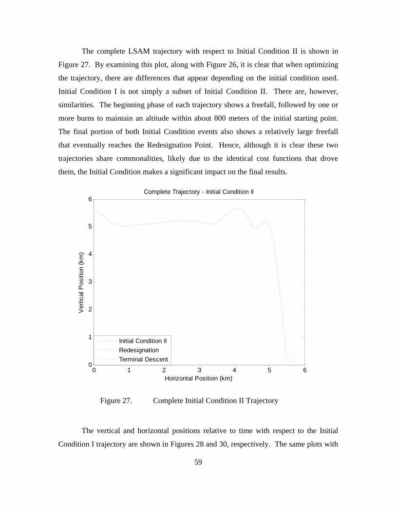
The complete LSAM trajectory with respect to Initial Condition II is shown in

Figure 27. By examining this plot, along with Figure 26, it is clear that when optimizing

the trajectory, there are differences that appear depending on the initial condition used.

Initial Condition I is not simply a subset of Initial Condition II. There are, however,

similarities. The beginning phase of each trajectory shows a freefall, followed by one or

more burns to maintain an altitude within about 800 meters of the initial starting point.

The final portion of both Initial Condition events also shows a relatively large freefall

that eventually reaches the Redesignation Point. Hence, although it is clear these two

trajectories share commonalities, likely due to the identical cost functions that drove

them, the Initial Condition makes a significant impact on the final results.

0 1 2 3 4 5 60

1

2

3

4

5

6Complete Trajectory - Initial Condition II


Ver

tical

Pos

ition

(km

)

Initial Condition II

Redesignation

Terminal Descent

Figure 27. Complete Initial Condition II Trajectory

The vertical and horizontal positions relative to time with respect to the Initial

Condition I trajectory are shown in Figures 28 and 30, respectively. The same plots with

59

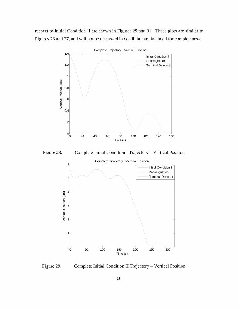
respect to Initial Condition II are shown in Figures 29 and 31. These plots are similar to

Figures 26 and 27, and will not be discussed in detail, but are included for completeness.

0 20 40 60 80 100 120 140 1600

0.2

0.4

0.6

0.8

1

1.2

1.4Complete Trajectory - Vertical Position

Time (s)

Ver

tical

Pos

ition

(km

)

Initial Condition I

Redesignation

Terminal Descent

Figure 28. Complete Initial Condition I Trajectory – Vertical Position

0 50 100 150 200 250 3000

1

2

3

4

5

6Complete Trajectory - Vertical Position

Time (s)

Ver

tical

Pos

ition

(km

)


Redesignation

Terminal Descent

Figure 29. Complete Initial Condition II Trajectory – Vertical Position

60

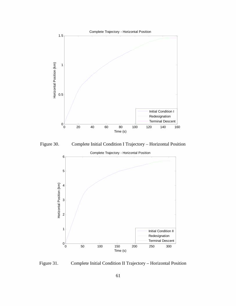
0 20 40 60 80 100 120 140 1600

0.5

1

1.5Complete Trajectory - Horizontal Position

Time (s)

Hor

izon

tal P

ositi

on (

km)

Initial Condition I

Redesignation

Terminal Descent

Figure 30. Complete Initial Condition I Trajectory – Horizontal Position

0 50 100 150 200 250 3000

1

2

3

4

5

6Complete Trajectory - Horizontal Position

Time (s)

Hor

izon

tal P

ositi

on (

km)


Redesignation

Terminal Descent

Figure 31. Complete Initial Condition II Trajectory – Horizontal Position

61

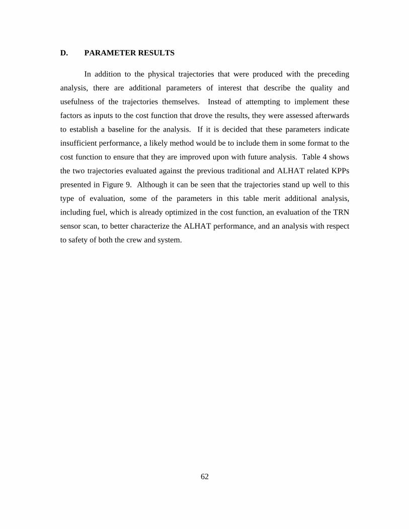
62

D. PARAMETER RESULTS

In addition to the physical trajectories that were produced with the preceding

analysis, there are additional parameters of interest that describe the quality and

usefulness of the trajectories themselves. Instead of attempting to implement these

factors as inputs to the cost function that drove the results, they were assessed afterwards

to establish a baseline for the analysis. If it is decided that these parameters indicate

insufficient performance, a likely method would be to include them in some format to the

cost function to ensure that they are improved upon with future analysis. Table 4 shows

the two trajectories evaluated against the previous traditional and ALHAT related KPPs

presented in Figure 9. Although it can be seen that the trajectories stand up well to this

type of evaluation, some of the parameters in this table merit additional analysis,

including fuel, which is already optimized in the cost function, an evaluation of the TRN

sensor scan, to better characterize the ALHAT performance, and an analysis with respect

to safety of both the crew and system.

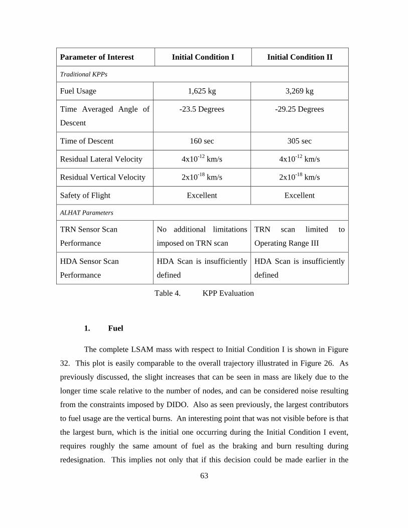
63

Parameter of Interest Initial Condition I Initial Condition II

Traditional KPPs

Fuel Usage 1,625 kg 3,269 kg

Time Averaged Angle of

Descent

-23.5 Degrees -29.25 Degrees

Time of Descent 160 sec 305 sec

Residual Lateral Velocity 4x10-12 km/s 4x10-12 km/s

Residual Vertical Velocity 2x10-18 km/s 2x10-18 km/s

Safety of Flight Excellent Excellent

ALHAT Parameters

TRN Sensor Scan

Performance

No additional limitations

imposed on TRN scan

TRN scan limited to

Operating Range III

HDA Sensor Scan

Performance

HDA Scan is insufficiently

defined

HDA Scan is insufficiently

defined

Table 4. KPP Evaluation

1. Fuel

The complete LSAM mass with respect to Initial Condition I is shown in Figure

32. This plot is easily comparable to the overall trajectory illustrated in Figure 26. As

previously discussed, the slight increases that can be seen in mass are likely due to the

longer time scale relative to the number of nodes, and can be considered noise resulting

from the constraints imposed by DIDO. Also as seen previously, the largest contributors

to fuel usage are the vertical burns. An interesting point that was not visible before is that

the largest burn, which is the initial one occurring during the Initial Condition I event,

requires roughly the same amount of fuel as the braking and burn resulting during

redesignation. This implies not only that if this decision could be made earlier in the

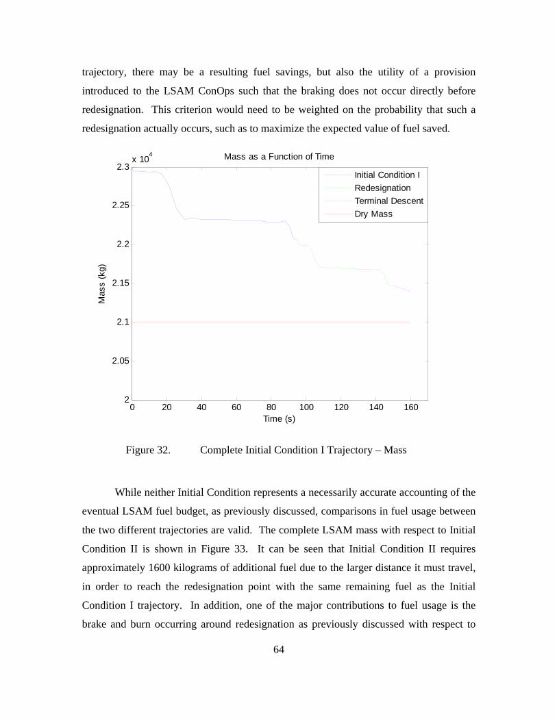
trajectory, there may be a resulting fuel savings, but also the utility of a provision

introduced to the LSAM ConOps such that the braking does not occur directly before

redesignation. This criterion would need to be weighted on the probability that such a

redesignation actually occurs, such as to maximize the expected value of fuel saved.

0 20 40 60 80 100 120 140 1602

2.05

2.1

2.15

2.2

2.25

2.3x 10


Time (s)

Mas

s (k

g)

Initial Condition I

Redesignation

Terminal Descent

Dry Mass

Figure 32. Complete Initial Condition I Trajectory – Mass

While neither Initial Condition represents a necessarily accurate accounting of the

eventual LSAM fuel budget, as previously discussed, comparisons in fuel usage between

the two different trajectories are valid. The complete LSAM mass with respect to Initial

Condition II is shown in Figure 33. It can be seen that Initial Condition II requires

approximately 1600 kilograms of additional fuel due to the larger distance it must travel,

in order to reach the redesignation point with the same remaining fuel as the Initial

Condition I trajectory. In addition, one of the major contributions to fuel usage is the

brake and burn occurring around redesignation as previously discussed with respect to

64

Initial Condition I. This further strengthens the point that additional analysis should be

completed to minimize this side effect of employing the ALHAT system.

0 50 100 150 200 250 3002

2.05

2.1

2.15

2.2

2.25

2.3

2.35

2.4

2.45

2.5x 10


Time (s)

Mas

s (k

g)


Redesignation

Terminal Descent

Dry Mass

Figure 33. Complete Initial Condition II Trajectory – Mass

2. TRN Sensor

The Terrain Relative Navigation phase is extremely important to the ALHAT

system. This is the first update of the state vector using local terrain data, which will

account for error in the location of the LSAM with respect to the intended landing site.

Reducing this error with an appropriate scan is extremely important, and the precise

requirements for altitude, duration and frequency of scan remain an open trade. As such,

in order to evaluate the TRN performance in this analysis, a required scan time of 60

seconds and three different Operating Ranges were considered, all of which is consistent

65

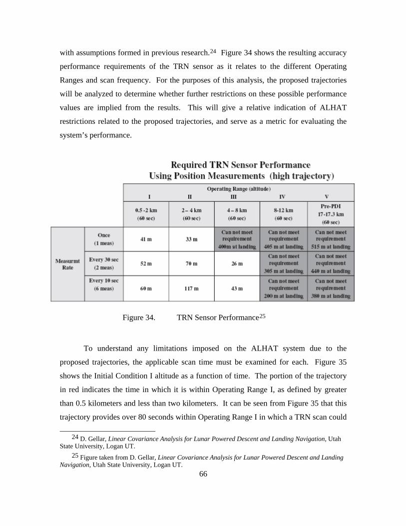
with assumptions formed in previous research.24 Figure 34 shows the resulting accuracy

performance requirements of the TRN sensor as it relates to the different Operating

Ranges and scan frequency. For the purposes of this analysis, the proposed trajectories

will be analyzed to determine whether further restrictions on these possible performance

values are implied from the results. This will give a relative indication of ALHAT

restrictions related to the proposed trajectories, and serve as a metric for evaluating the

system’s performance.

Figure 34. TRN Sensor Performance25

To understand any limitations imposed on the ALHAT system due to the

proposed trajectories, the applicable scan time must be examined for each. Figure 35

shows the Initial Condition I altitude as a function of time. The portion of the trajectory

in red indicates the time in which it is within Operating Range I, as defined by greater

than 0.5 kilometers and less than two kilometers. It can be seen from Figure 35 that this

trajectory provides over 80 seconds within Operating Range I in which a TRN scan could

24 D. Gellar, Linear Covariance Analysis for Lunar Powered Descent and Landing Navigation, Utah

State University, Logan UT.

66

25 Figure taken from D. Gellar, Linear Covariance Analysis for Lunar Powered Descent and Landing Navigation, Utah State University, Logan UT.

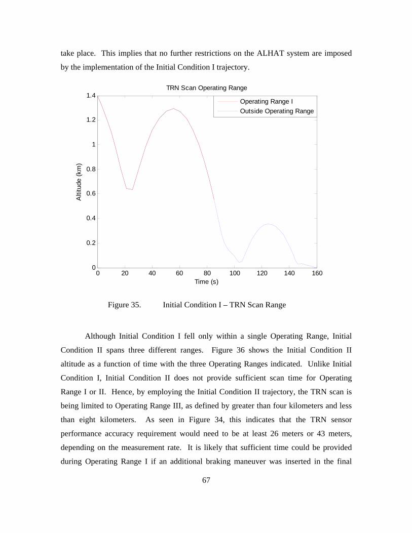
take place. This implies that no further restrictions on the ALHAT system are imposed

by the implementation of the Initial Condition I trajectory.

0 20 40 60 80 100 120 140 1600

0.2

0.4

0.6

0.8

1

1.2

1.4

Time (s)

Alti

tude

(km

)

TRN Scan Operating Range

Operating Range I

Outside Operating Range

Figure 35. Initial Condition I – TRN Scan Range

Although Initial Condition I fell only within a single Operating Range, Initial

Condition II spans three different ranges. Figure 36 shows the Initial Condition II

altitude as a function of time with the three Operating Ranges indicated. Unlike Initial

Condition I, Initial Condition II does not provide sufficient scan time for Operating

Range I or II. Hence, by employing the Initial Condition II trajectory, the TRN scan is

being limited to Operating Range III, as defined by greater than four kilometers and less

than eight kilometers. As seen in Figure 34, this indicates that the TRN sensor

performance accuracy requirement would need to be at least 26 meters or 43 meters,

depending on the measurement rate. It is likely that sufficient time could be provided

during Operating Range I if an additional braking maneuver was inserted in the final

67

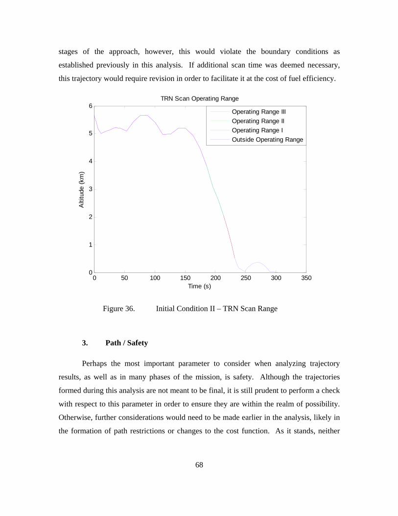
stages of the approach, however, this would violate the boundary conditions as

established previously in this analysis. If additional scan time was deemed necessary,

this trajectory would require revision in order to facilitate it at the cost of fuel efficiency.

0 50 100 150 200 250 300 3500

1

2

3

4

5

6

Time (s)

Alti

tude

(km

)

TRN Scan Operating Range

Operating Range III

Operating Range II

Operating Range I

Outside Operating Range

Figure 36. Initial Condition II – TRN Scan Range

3. Path / Safety

Perhaps the most important parameter to consider when analyzing trajectory

results, as well as in many phases of the mission, is safety. Although the trajectories

formed during this analysis are not meant to be final, it is still prudent to perform a check

with respect to this parameter in order to ensure they are within the realm of possibility.

Otherwise, further considerations would need to be made earlier in the analysis, likely in

the formation of path restrictions or changes to the cost function. As it stands, neither

68

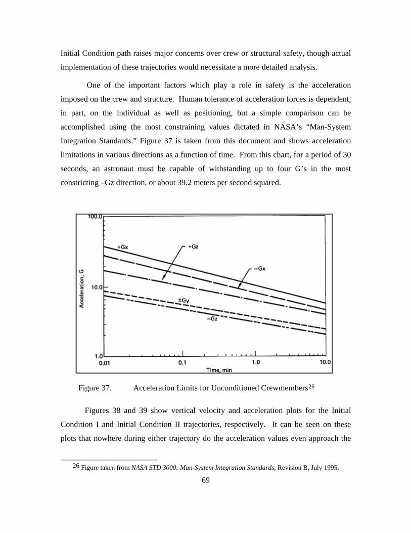
Initial Condition path raises major concerns over crew or structural safety, though actual

implementation of these trajectories would necessitate a more detailed analysis.

One of the important factors which play a role in safety is the acceleration

imposed on the crew and structure. Human tolerance of acceleration forces is dependent,

in part, on the individual as well as positioning, but a simple comparison can be

accomplished using the most constraining values dictated in NASA’s “Man-System

Integration Standards.” Figure 37 is taken from this document and shows acceleration

limitations in various directions as a function of time. From this chart, for a period of 30

seconds, an astronaut must be capable of withstanding up to four G’s in the most

constricting –Gz direction, or about 39.2 meters per second squared.

Figure 37. Acceleration Limits for Unconditioned Crewmembers26

Figures 38 and 39 show vertical velocity and acceleration plots for the Initial

Condition I and Initial Condition II trajectories, respectively. It can be seen on these

plots that nowhere during either trajectory do the acceleration values even approach the

26 Figure taken from NASA STD 3000: Man-System Integration Standards, Revision B, July 1995.

69

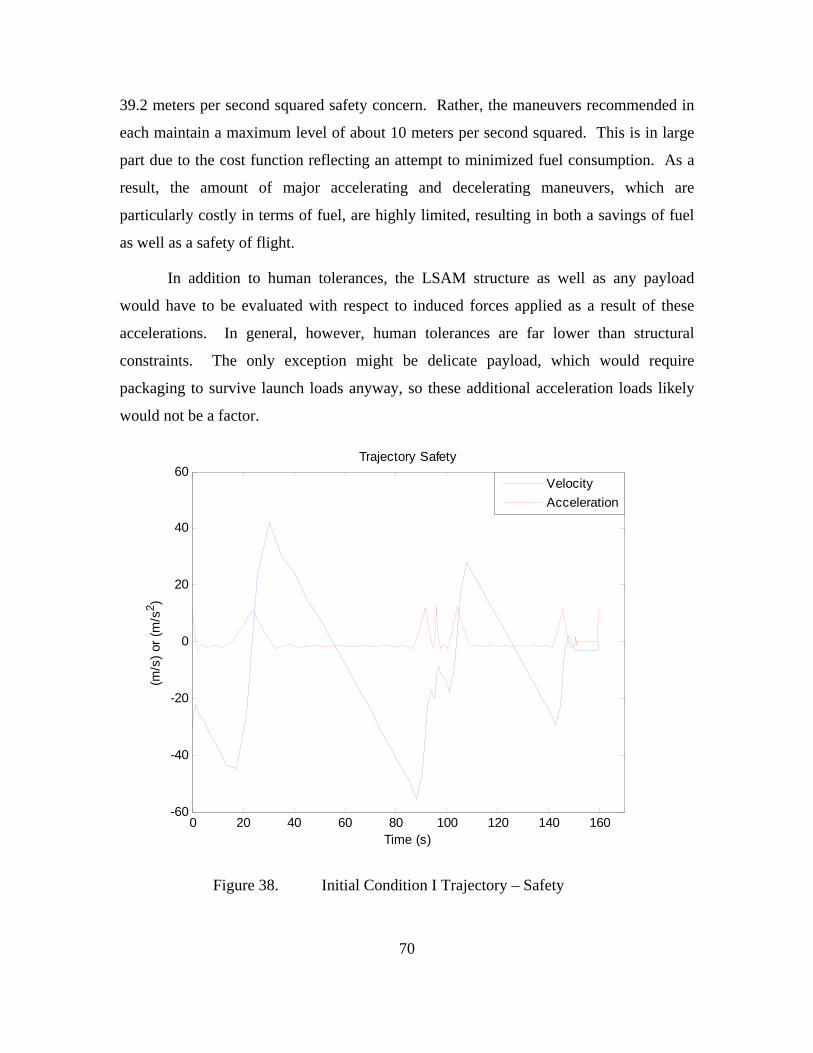
39.2 meters per second squared safety concern. Rather, the maneuvers recommended in

each maintain a maximum level of about 10 meters per second squared. This is in large

part due to the cost function reflecting an attempt to minimized fuel consumption. As a

result, the amount of major accelerating and decelerating maneuvers, which are

particularly costly in terms of fuel, are highly limited, resulting in both a savings of fuel

as well as a safety of flight.

In addition to human tolerances, the LSAM structure as well as any payload

would have to be evaluated with respect to induced forces applied as a result of these

accelerations. In general, however, human tolerances are far lower than structural

constraints. The only exception might be delicate payload, which would require

packaging to survive launch loads anyway, so these additional acceleration loads likely

would not be a factor.

0 20 40 60 80 100 120 140 160-60

-40

-20

0

20

40

60Trajectory Safety

Time (s)

(m/s

) or

(m

/s2 )

Velocity

Acceleration

Figure 38. Initial Condition I Trajectory – Safety

70

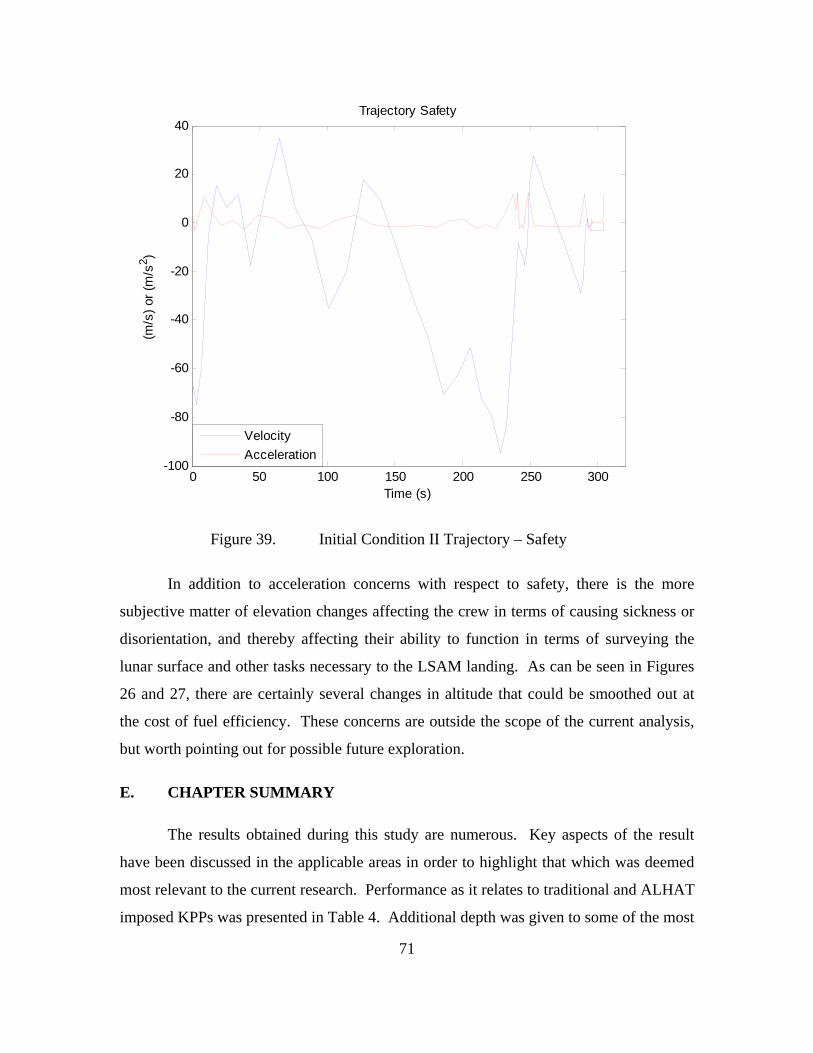
0 50 100 150 200 250 300-100

-80

-60

-40

-20

0

20

40Trajectory Safety

Time (s)

(m/s

) or

(m

/s2 )

Velocity

Acceleration

Figure 39. Initial Condition II Trajectory – Safety

In addition to acceleration concerns with respect to safety, there is the more

subjective matter of elevation changes affecting the crew in terms of causing sickness or

disorientation, and thereby affecting their ability to function in terms of surveying the

lunar surface and other tasks necessary to the LSAM landing. As can be seen in Figures

26 and 27, there are certainly several changes in altitude that could be smoothed out at

the cost of fuel efficiency. These concerns are outside the scope of the current analysis,

but worth pointing out for possible future exploration.

E. CHAPTER SUMMARY

The results obtained during this study are numerous. Key aspects of the result

have been discussed in the applicable areas in order to highlight that which was deemed

most relevant to the current research. Performance as it relates to traditional and ALHAT

imposed KPPs was presented in Table 4. Additional depth was given to some of the most

71

72

important parameters of interest in order to help evaluate the trajectories with respect to

something other than the optimized cost function. This analysis is not meant to be a

completely inclusive summary of all results, simply those that were most important to the

scope of the study. Additional analysis may show trends that could be iterated on or

explored further. In the following chapter, suggestions will be made to adapt the

methodologies used during this study in order to produce even more applicable results.

In addition, areas of future research will be highlighted, which are indicated by the data

presented in this chapter.

73

VI. CONCLUSIONS

A. METHODOLOGIES AND RECOMMENDATIONS

The results of the optimization presented in the previous chapter provide a variety

of data that may be further analyzed and scrutinized. From it, however, and with respect

to the initial questions posed by this thesis, there are a few key points that should be

considered, and some methods that could be expanded in future iterations. In addition to

those points and methodologies, future recommendations can be made to guide ongoing

areas of research. As noted previously, numerous trades with respect to both the ALHAT

system and LSAM remain open, and any conclusions may prove useful in providing

some modicum of direction in exploring these trade spaces.

1. DIDO Utility

One of the unique aspects of this research was the implementation of DIDO to

optimize the trajectories. Although this method carried with it some associated

constraints, it was overall extremely useful in the analysis. The ability to easily code and

modify the problem statement with the DIDO associated Matlab scripts allowed for

versatility in establishing the parameters and examining the results. By using DIDO as

opposed to an algorithm that simply perpetuates the state variables, the trajectory and its

parameters were optimized over the entire event timeline, rather than through a series of

finite points, yielding both a high degree of accuracy with respect to the cost function, as

well as a simplistic interface to work with. DIDO’s versatility to accommodate a unique

trade space and overall utility make it an optimal method to employ in future studies of

this nature.

The constraints imposed by DIDO, as discussed in the previous chapter, were

largely a product of the version of code used. In order to overcome many of these issues,

the professional version of DIDO could be obtained. By doing so, future analysis with

respect to lunar landing trajectories or the ALHAT system would not only be made

computationally easier, but would maintain a basis in the current results. A study could

74

also be done to understand the effects of the constraints described in the current analysis.

In addition to overcoming some of the physical constraints associated with the limited

version of DIDO, the professional version could also allow for an expansion of the

parameters examined during the analysis.

2. Modeling Parameters

The current analysis included many of the most important parameters regarding

both the lunar landing trajectory as well as the ALHAT system. However, there are other

variables that could be introduced in order to expand the understanding of the results, as

well as modifications that could be made in order to make the model more complex and

akin to real life. Because the current analysis focused on providing a foundation for

future research and implementing methods that had not been previously utilized, there is

certainly room for expansion on this established baseline.

Some additional complexities that could be considered in future research include

an expansion on the cursory safety analysis. Stress loads applicable to both human

tolerances as well as structural integrity concerns require more in depth attention to

ensure there are no safety of flight concerns. In addition, a further refinement of the

mass analysis could be performed once the LSAM design is more mature.

Considerations such as fuel reserves and maneuver margins could significantly impact

the overall mass in this area. Finally, an inclusion of certain parameters such as induced

drag and three dimensional movement would add an additional layer of complexity, and

thereby realism to the analysis.

In addition to these parameters, there are certain modeling efforts that could be

examined or changed. The vertical angle of attack restriction imposed in an effort to

segregate horizontal and vertical planes could be removed with the development of the

problem statement on the professional version of DIDO. With this implementation come

angle restrictions that will affect thrust levels and sensor scan angles, which were not an

issue in the current analysis. In addition, the trajectory itself could be modeled

differently, as previously discussed findings indicate that altering the boundary

conditions or duration of the path itself can vastly affect the results. Certainly there is a

75

substantial difference simply in considering the Initial Condition I versus Initial

Condition II trajectories, indicating the importance of selecting only that portion of the

trajectory that should be optimized with respect to the particular cost function.

3. ALHAT Considerations

In addition to the expansion of methods that could provide additional insight into

the current research, revisions with regard to the ALHAT system could be made as the

system design matures. For instance, in the current analysis, a redesignation point of 210

meters down range was chosen as a point of study. Some research, however, suggests a

maximum redesignation distance of two kilometers up or down range may be required.27

This would certainly affect the resulting trajectory, as would a more detailed

representation of the terrain or the additional complexity of implementing a three

dimensional landing area. Inclusion of these factors could help to evaluate the expected

performance of the ALHAT as well as the LSAM in these limiting cases.

Evaluation of the ALHAT system can also be refined in future analysis.

Currently, the TRN and HDA sensors are areas of open trade for the system, and as these

areas are refined, and requirements flushed out, the evaluation of their expected

performance can be updated as well. The HDA sensor, for example, has yet to advance

to a significantly mature stage of development to even allow constructing reasonable

evaluation criteria to be possible, as shown in Table 4. Research with respect to these

technologies’ requirements, however, can help to drive their development, and so it is an

iterative and cyclical process. Besides the evaluation of these technologies, the manner

of their implementation can also be refined. The balance between reliance on human

control and sensor guidance is an important one, especially as technology progresses.

These trades can be explored as well simply by modeling them differently in related

DIDO optimization analysis.



76

B. AREAS FOR FUTURE RESEARCH

Although there are a great number of alterations in methodology and additional

complexities that could be included in future analysis, there are three specific areas of

continued research that the current baseline research suggests. The first of these areas is

the rigorous development of an accurate and reflective cost function with which to drive

the DIDO optimization. This tool can be used simply to show an ideal trajectory which

minimizes fuel expenditure as was accomplished here, but the potential exists to perform

a complex series of system level trades, so long as the relationship between the

parameters can be well understood and modeled. Rather than exploring a multi-faceted

system level trade space in order to find the maximizing combination of variables, DIDO

can demonstrate this ideal directly, as long as the effort has been made to accurately

reflect the importance of such parameters and their relationship to each other. This

represents a great deal of utility to the system engineer that can incorporate DIDO, not

simply with respect to trajectory analysis, but any facet of study, and as such, is

recommended for a direct area of pursuit for additional research.

Along with the continued exploration of DIDO’s utility, a recommendation to

further examine a feature this method uncovered is warranted. In both the Initial

Condition I and Initial Condition II trajectories, the primary operating range for TRN

scan was centralized at the beginning of the event timeline. Although these two

trajectories began at different positions, the indication is clear that from a fuel efficiency

perspective, the time to initiate this scan is at the beginning of whatever trajectory one

chooses. Therefore, further research is justified in the area of early TRN scan

requirements and performance.

Finally, the third area of additional research motivated by the current analysis is in

the area of braking maneuvers prior to ALHAT redesignation. Specifically, this would

comprise of further study in optimized ConOps with respect to the utilization of a partial

braking maneuver just prior to a possible landing site redesignation. As previously

discussed, if the braking maneuver is scaled by the probability that a redesignation takes

place, it is likely possible to stochastically optimize the current trajectory with respect to

77

a probabilistically determined expected value as opposed to a deterministic model. This

would provide for a maximum fuel efficiency founded in the probability of a

redesignation, rather than the assumption that one will occur, and therefore be more

accurate over time. This would also represent a specific change to LSAM landing

ConOps dictated by the inclusion of the ALHAT system.

78


79

LIST OF REFERENCES

Curtis, Howard D. Orbital Mechanics for Engineering Students. Butterworth-Heinemann, 2005.

Epp, Chirold et al. Autonomous Landing and Hazard Avoidance Technology (ALHAT). Johnson Space Center. Houston, TX.

Gellar, D. Linear Covariance Analysis for Lunar Powered Descent and Landing Navigation. Utah State University, Logan UT.

Godwin, Robert, ed. Apollo 11 – The NASA Mission Reports. Apogee Books, 1999.

IEEEAC paper #1643, Version 5, Updated December 17, 2007.

Johnson, Andrew E. et al. Analysis of On-Boad Hazard Detection and Avoidance for Safe Lunar Landing. Jet Propulsion Laboratory, California Institute of Technology, Pasadena, CA.

Klumpp, Allan R. Apollo Lunar-Descent Guidance. Charles Stark Draper Laboratory, R-695, June 1971.

M. Ross and F. Fahroo. A Perspective on Methods for Trajectory Optimization. AIAA/AAS Astrodynamics Specialist Conf., Monterey, 2002.

NASA STD 3000: Man-System Integration Standards. Revision B, July 1995.

NASA’s Exploration Systems Architecture Study. November 2005. Online. Available at www.sti.nasa.gov. Accessed July 17, 2009.

Paschall, Steve et al. A Self Contained Method for Safe & Precise Lunar Landing. NASA Johnson Space Center, Houston, TX.

Ronald Sostaric and Jeremy Rea. Powered Descent Guidance Methods for the Moon and Mars. Johnson Space Center, Houston, Tx.

Ross, I. and F. Fahroo. Legendre Pseudospectral Approximations of Optimal Control Problems. Naval Postgraduate School, Monterey, CA 2003.

Smithsonian National Air and Space Museum website. Online. Available at http://www.nasm.si.edu/collections/imagery/apollo/AS11/a11landsite.htm. Accessed July 17, 2009.

Sostaric, Ronald R. Powered Descent Trajectory Guidance and some Considerations for Human Lunar Landing. NASA Johnson Space Center. Houston, TX.

Wertz, James R. and Wiley Larson, eds. Space Mission Analysis and Design. Torrance, CA: Microcosm Press, 1999.


80


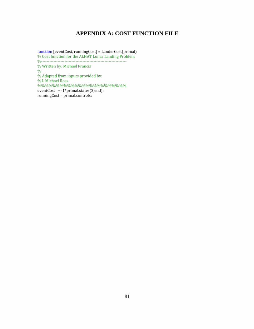
81

APPENDIX A: COST FUNCTION FILE

function [eventCost, runningCost] = LanderCost(pri Lunar Landing Prob‐‐‐‐‐‐‐‐‐‐‐‐‐‐‐‐‐‐‐‐‐‐‐‐‐

mal)lem

% Cost function for the ALHAT‐‐‐‐‐‐‐‐‐‐‐‐‐‐‐‐‐‐‐‐‐‐‐‐‐‐‐‐‐‐‐‐‐‐‐‐%‐

% Written by: Michael Francis % % Adapted from inputs provided by:

%%%%% % I. Michael Ross

%%%%,end);

%%%%%%%%%%%%%%%ventCost = ‐1*primal.states(3unningCost = primal.controls; er

82


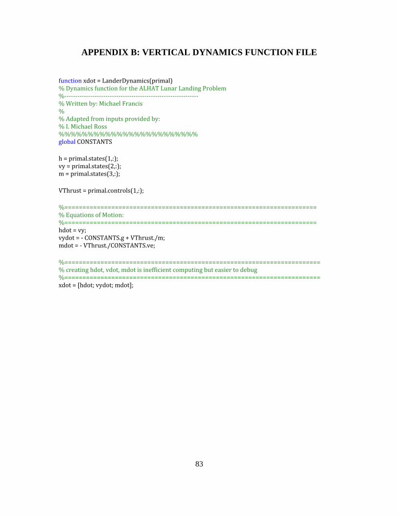
83

APPENDIX B: VERTICAL DYNAMICS FUNCTION FILE

function xdot = LanderDynamics(primal) HAT Lunar Landing‐‐‐‐‐‐‐‐‐‐‐‐‐‐‐‐‐‐‐‐‐‐‐‐‐

% Dynamics function for the AL‐‐‐‐‐‐‐‐‐‐‐‐‐‐‐‐‐‐‐‐‐‐‐‐‐‐‐‐‐‐‐‐‐‐‐‐

Problem %‐% Written by: Michael Francis % % Adapted from inputs provided by:

%%%%%%%%%%%%%% % I. Michael Ross %%%%%%%%%%

global CONSTANTS

h = primal.states(1,:); y = primal.states(2,:); vm = primal.states(3,:); VThrust = primal.controls(1,:); %======================================================================

s of Motion: =======================================

% Equation%===============================

m; hdot = vy; ydot = ‐ CONSTANTS.g + VThrust./vmdot = ‐ VThrust./CONSTANTS.ve; %=======================================================================

is inefficient computing but easier to debug ===================================================

% creating hdot, vdot, mdot%====================xdot = [hdot; vydot; mdot];

84


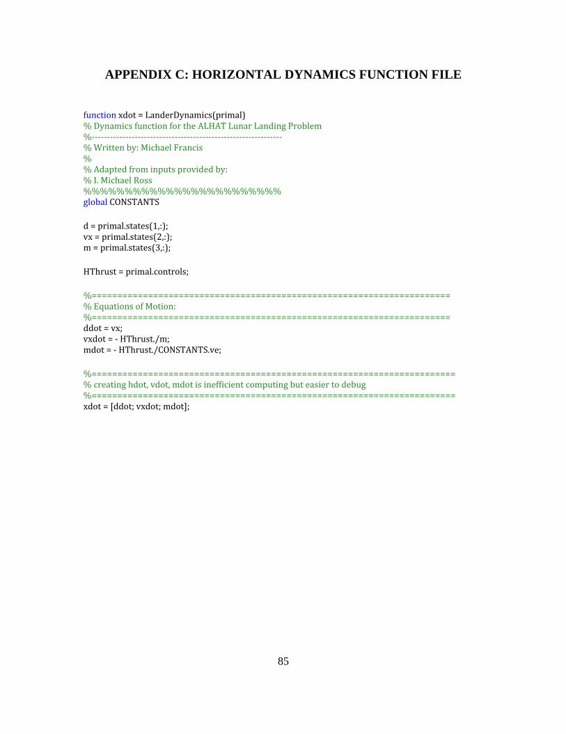
85

APPENDIX C: HORIZONTAL DYNAMICS FUNCTION FILE

function xdot = LanderDynamics(primal) HAT Lunar Landing‐‐‐‐‐‐‐‐‐‐‐‐‐‐‐‐‐‐‐‐‐‐‐‐‐

% Dynamics function for the AL‐‐‐‐‐‐‐‐‐‐‐‐‐‐‐‐‐‐‐‐‐‐‐‐‐‐‐‐‐‐‐‐‐‐‐‐

Problem %‐% Written by: Michael Francis % % Adapted from inputs provided by:

%%%%%%%%%%%%%% % I. Michael Ross %%%%%%%%%%

global CONSTANTS

d = primal.states(1,:); x = primal.states(2,:); vm = primal.states(3,:); HThrust = primal.controls; %======================================================================

ns of Motion: ======================================================

% Equatio%================ddot = vx; xdot = ‐ HThrust./m; vmdot = ‐ HThrust./CONSTANTS.ve; %=======================================================================

is inefficient computing but easier to debug ===================================================

% creating hdot, vdot, mdot%====================xdot = [ddot; vxdot; mdot];

86


87

APPENDIX D: EVENTS FUNCTION FILE

function eventConditions = LanderEvents(primal) T Lundar Landing P‐‐‐‐‐‐‐‐‐‐‐‐‐‐‐‐‐‐‐‐‐‐‐‐‐

% Events function for the ALHA‐‐‐‐‐‐‐‐‐‐‐‐‐‐‐‐‐‐‐‐‐‐‐‐‐‐‐‐‐‐‐‐‐‐‐‐

roblem %‐% Written by: Michael Francis % % Adapted from inputs provided by:

%%%%%%%%%%%%%% % I. Michael Ross %%%%%%%%%%

global CONSTANTS h0 = primal.states(1,1); hf = primal.states(1,end); y0 = primal.states(2,1); vyf = primal.states(2,end); vm0 = primal.states(3,1); mf = primal.states(3,end);

ions (i.e. event conditions) for good MATLAB computing % preallocate boundary condit eventConditions = zeros(5, 1);

======================================== %===================eventConditions(1) = h0; eventConditions(2) = vy0;

; ‐‐‐‐‐‐‐‐‐‐‐‐‐‐‐‐‐‐‐‐‐‐‐‐‐‐‐‐

eventConditions(3) = m0%‐‐‐‐‐‐‐‐‐‐‐‐‐‐‐‐‐‐‐‐‐‐‐‐‐‐‐‐‐‐‐eventConditions(4) = hf; eventConditions(5) = vyf; %===========================================================

88


bb

89

APPENDIX E: INITIAL CONDITION I PROBLEM FILE

% Problem File for the ALHAT ‐‐‐‐‐‐‐‐‐‐‐‐‐‐‐‐‐‐‐‐‐‐‐‐‐‐‐‐‐‐‐‐‐‐‐‐

Lunar Landing Probl‐‐‐‐‐‐‐‐‐‐‐‐‐‐‐‐‐‐‐‐‐‐‐‐‐

em %‐% Written by: Michael Francis % % Adapted from inputs provided by:

% I. Michael Ross %%%%%%%%%%%%%%%%%%%%%%%%

===================== clear all; ==============%

global CONSTANTS CONSTANTS.g = 0.001622; %km/s^2 % g of moon ONSTANTS.ve = 4.25; %km/s % exhaust velocity

%kN = kgkm/s^2 % all are in normalized units CCONSTANTS.Tmax = 4*66.7;

%‐‐‐‐‐‐‐‐‐‐‐‐‐‐‐‐‐‐‐‐‐‐‐‐‐‐‐‐‐‐‐‐‐‐‐ % Define the problem function files:%‐‐‐‐‐‐‐‐‐‐‐‐‐‐‐‐‐‐‐‐‐‐‐‐‐‐‐‐‐‐‐‐‐‐‐

; ALHAT.cost = 'verALHATCost';

verALHATDynamics'rALHATEvents';

ALHAT.dynamics = 'LHAT.events = 'veA

% no path constraints

LED units %‐‐‐‐‐‐‐‐‐‐‐‐‐‐‐‐‐‐‐‐‐‐‐‐‐‐‐‐‐‐‐‐‐‐‐‐‐‐‐‐‐‐‐ Set up the problem bounds in SCA%

%‐‐‐‐‐‐‐‐‐‐‐‐‐‐‐‐‐‐‐‐‐‐‐‐‐‐‐‐‐‐‐‐‐‐‐‐‐‐‐‐‐‐‐

ot choose Inf tfMax = 200; % large upper bound; do n

ounds.lower.time = [0 95.5]; %95.5bbounds.upper.time = [0 95.5];

km km/s kg 0 = 1.4; vy0 = ‐0.03; m0 = 23000; % initial conditions ‐ units

tions hhf = 0.15; vyf = ‐0.02; mfmin = 21000; % boundary condi

se the equations Note: DO NOT set mfmin to zero becau

%% of motion have a singularity at m = 0.

]; ounds.lower.states = [ 0; ‐10; mfmin

10; m0]; bbounds.upper.states = [ 2.5; ounds.lower.controls = 0; bbounds.upper.controls = CONSTANTS.Tmax;

ounds.lower.events = [h0; vy0; m0; hf; vyf]; ounds.upper.events = bounds.lower.events;

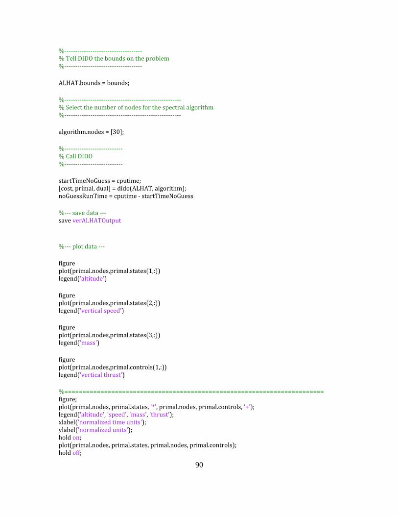
hold on; plot(primhold off;

90

ylabel('normalized units');

al.nodes, primal.states, primal.nodes, primal.controls);

%‐‐‐‐‐‐‐‐‐‐‐‐‐‐‐‐‐‐‐‐‐‐‐‐‐‐‐‐‐‐‐‐‐‐‐‐ Tell DIDO the bounds on the

‐‐‐‐‐ % problem %‐‐‐‐‐‐‐‐‐‐‐‐‐‐‐‐‐‐‐‐‐‐‐‐‐‐‐‐‐‐‐ ALHAT.bounds = bounds;

l algorithm %‐‐‐‐‐‐‐‐‐‐‐‐‐‐‐‐‐‐‐‐‐‐‐‐‐‐‐‐‐‐‐‐‐‐‐‐‐‐‐‐‐‐‐‐‐‐‐‐‐‐‐‐‐‐ Select the number of nodes for the spectra

‐‐‐‐‐‐‐‐‐‐‐‐‐‐‐‐‐‐‐‐‐‐‐‐ %%‐‐‐‐‐‐‐‐‐‐‐‐‐‐‐‐‐‐‐‐‐‐‐‐‐‐‐‐‐‐

algorithm.nodes = [30]; %‐‐‐‐‐‐‐‐‐‐‐‐‐‐‐‐‐‐‐‐‐‐‐‐‐‐‐ Call DIDO %

%‐‐‐‐‐‐‐‐‐‐‐‐‐‐‐‐‐‐‐‐‐‐‐‐‐‐‐ startTimeNoGuess = cputime; ost, primal, dual] = dido(ALHAT, algorithm);

= cputime ‐ startTimeNoGuess [cnoGuessRunTime ‐‐‐ save data ‐‐‐ ave verALHATOutput %s

ot data ‐‐‐ %‐‐‐ pl

,primal.states(1,:)) figure lot(primal.nodes

('altitude') plegend

l.states(2,:)) figure lot(primal.nodes,prima

('vertical speed') plegend

es,primal.states(3,:)) figure lot(primal.nod

('mass') plegend

l.controls(1,:)) figure lot(primal.nodes,primaplegend('vertical thrust')

============== %==========================================================

l.nodes, primal.controls, '+'); figure;

'*', prima'thrust');

plot(primal.nodes, primal.states,ass', its');

legend('altitude', 'speed', 'mormalized time unxlabel('n

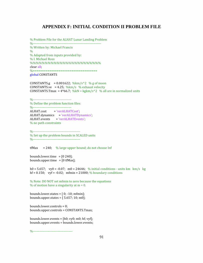
bounds.upper.events = bounds %‐‐‐‐‐‐‐‐‐‐‐‐‐‐‐‐‐‐‐‐‐‐‐‐‐‐‐‐‐‐‐‐‐‐‐‐

91

APPENDIX F: INITIAL CONDITION II PROBLEM FILE

% Problem File for the ALHAT ‐‐‐‐‐‐‐‐‐‐‐‐‐‐‐‐‐‐‐‐‐‐‐‐‐‐‐‐‐‐‐‐‐‐‐‐

Lunar Landing Probl‐‐‐‐‐‐‐‐‐‐‐‐‐‐‐‐‐‐‐‐‐‐‐‐‐

em %‐% Written by: Michael Francis % % Adapted from inputs provided by:

% I. Michael Ross %%%%%%%%%%%%%%%%%%%%%%%%

===================== clear all; ==============%

global CONSTANTS CONSTANTS.g = 0.001622; %km/s^2 % g of moon ONSTANTS.ve = 4.25; %km/s % exhaust velocity

%kN = kgkm/s^2 % all are in normalized units CCONSTANTS.Tmax = 4*66.7;

%‐‐‐‐‐‐‐‐‐‐‐‐‐‐‐‐‐‐‐‐‐‐‐‐‐‐‐‐‐‐‐‐‐‐‐ % Define the problem function files:%‐‐‐‐‐‐‐‐‐‐‐‐‐‐‐‐‐‐‐‐‐‐‐‐‐‐‐‐‐‐‐‐‐‐‐

; ALHAT.cost = 'verALHATCost';

verALHATDynamics'rALHATEvents';

ALHAT.dynamics = 'LHAT.events = 'veA

% no path constraints

LED units %‐‐‐‐‐‐‐‐‐‐‐‐‐‐‐‐‐‐‐‐‐‐‐‐‐‐‐‐‐‐‐‐‐‐‐‐‐‐‐‐‐‐‐ Set up the problem bounds in SCA%

%‐‐‐‐‐‐‐‐‐‐‐‐‐‐‐‐‐‐‐‐‐‐‐‐‐‐‐‐‐‐‐‐‐‐‐‐‐‐‐‐‐‐‐

d; do not choose Inf tfMax = 240; % large upper boun ounds.lower.time = [0 240]; bbounds.upper.time = [0 tfMax];

s km km/s kg 0 = 5.657; vy0 = ‐0.07; m0 = 24646; % initial conditions ‐ unit

ditions hhf = 0.150; vyf = ‐0.02; mfmin = 21000; % boundary con

se the equations Note: DO NOT set mfmin to zero becau

%% of motion have a singularity at m = 0. ounds.lower.states = [ 0; ‐10; mfmin];

bbounds.upper.states = [ 5.657; 10; m0]; ounds.lower.controls = 0; bbounds.upper.controls = CONSTANTS.Tmax;

ounds.lower.events = [h0; vy0; m0; hf; vyf];

.lower.events; b

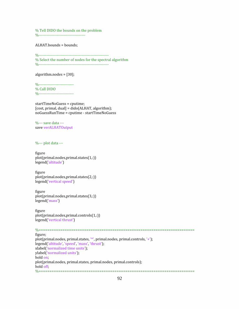
92

plot(primal.nodes, primal.states, primal.nodes, primal.controls); hold off; %========================================================================

% Tell DIDO the bounds on the‐‐‐‐‐

problem %‐‐‐‐‐‐‐‐‐‐‐‐‐‐‐‐‐‐‐‐‐‐‐‐‐‐‐‐‐‐‐ ALHAT.bounds = bounds;

l algorithm %‐‐‐‐‐‐‐‐‐‐‐‐‐‐‐‐‐‐‐‐‐‐‐‐‐‐‐‐‐‐‐‐‐‐‐‐‐‐‐‐‐‐‐‐‐‐‐‐‐‐‐‐‐‐ Select the number of nodes for the spectra

‐‐‐‐‐‐‐‐‐‐‐‐‐‐‐‐‐‐‐‐‐‐‐‐ %%‐‐‐‐‐‐‐‐‐‐‐‐‐‐‐‐‐‐‐‐‐‐‐‐‐‐‐‐‐‐

algorithm.nodes = [30]; %‐‐‐‐‐‐‐‐‐‐‐‐‐‐‐‐‐‐‐‐‐‐‐‐‐‐‐ Call DIDO %

%‐‐‐‐‐‐‐‐‐‐‐‐‐‐‐‐‐‐‐‐‐‐‐‐‐‐‐ startTimeNoGuess = cputime; ost, primal, dual] = dido(ALHAT, algorithm);

= cputime ‐ startTimeNoGuess [cnoGuessRunTime ‐‐‐ save data ‐‐‐ ave verALHATOutput %s

ot data ‐‐‐ %‐‐‐ pl

,primal.states(1,:)) figure lot(primal.nodes

('altitude') plegend

l.states(2,:)) figure lot(primal.nodes,prima

('vertical speed') plegend

es,primal.states(3,:)) figure lot(primal.nod

('mass') plegend

l.controls(1,:)) figure lot(primal.nodes,primaplegend('vertical thrust')

============== %==========================================================

l.nodes, primal.controls, '+'); figure;

'*', prima'thrust');

plot(primal.nodes, primal.states,ass', its');

legend('altitude', 'speed', 'mormalized time unxlabel('n

ylabel('normalized units'); hold on;

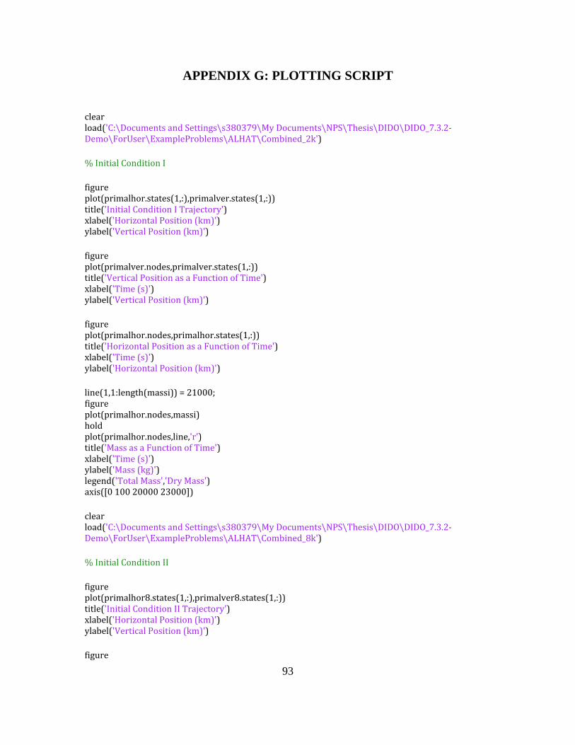
ylabel( figure

93

APPENDIX G: PLOTTING SCRIPT

clear ad('C:\Documents and Settings\s380379\My Documents\NPS\Thesis\DIDO\DIDO_7.3.2‐

pleProblems\ALHAT\Combined_2k') loDemo\ForUser\Exam

al Condition I % Initi

states(1,:)) figure

r.)

plot(primalhor.states(1,:),primalvery')')

title('Initial Condition I Trajectolabel('Horizontal Position (km

'Vertical Position (km)') xylabel( figure

des,primalver.states(1,:)) tion of Time')

plot(primalver.notitle('Vertical Position as a Funclabel('Time (s)')


des,primalhor.states(1,:)) tion of Time')

plot(primalhor.notitle('Horizontal Position as a Funclabel('Time (s)')

xylabel('Horizontal Position (km)')

00; line(1,1:length(massi)) = 210

figureplot(primalhor.nodes,massi) hold

des,line,'r') ction of Time')

plot(primalhor.notitle('Mass as a Funxlabel('Time (s)')

ss') ylabel('Mass (kg)') gend('Total Mass','Dry Ma

0 100 20000 23000]) leaxis([ clear ad('C:\Documents and Settings\s380379\My Documents\NPS\Thesis\DIDO\DIDO_7.3.2‐

pleProblems\ALHAT\Combined_8k') loDemo\ForUser\Exam

al Condition II % Initi

8.states(1,:)) figure

er')

plot(primalhor8.states(1,:),primalvry)')

title('Initial Condition II Trajectolabel('Horizontal Position (km

'Vertical Position (km)') x

hold plot(primalhorredes.nodes,line,'r')title('Mass as a Function of Time')

94

plot(primalver8.nodes,primalver8.states(1,:))tion of Time')

title('Vertical Position as a Funclabel('Time (s)')


odes,primalhor8.states(1,:)) tion of Time')

plot(primalhor8.ntitle('Horizontal Position as a Funclabel('Time (s)')

xylabel('Horizontal Position (km)')

0; line(1,1:length(massi)) = 2100

figureplot(primalhor8.nodes,massi) hold

odes,line,'r') ction of Time')

plot(primalhor8.ntitle('Mass as a Funxlabel('Time (s)')

ss') ylabel('Mass (kg)') gend('Total Mass','Dry Ma


eProblems\ALHAT\Combined_2k') loDemo\ForUser\Exampl

esignation Point % Red

erredes.states(1,:)) figure

malvry')

plot(primalhorredes.states(1,:),pricto)')

title('Redesignation Point Trajelabel('Horizontal Position (km

'Vertical Position (km)') xylabel(

tes(1,:)) figure

es.nodes,primalverredes.station of Time')

plot(primalverredtitle('Vertical Position as a Funclabel('Time (s)')


(1,:)) figure

es.nodes,primalhorredes.statestion of Time')

plot(primalhorredtitle('Horizontal Position as a Funclabel('Time (s)')

xylabel('Horizontal Position (km)') line(1,1:length(massr)) = 21000;

figureplot(primalhorredes.nodes,massr)

figure plot(primalver.nodes(1,:),primalver.states(1,:))

95

xlabel('Time (s)')

ass') ylabel('Mass (kg)') gend('Total Mass','Dry M

00]) leaxis([0 60 20000 225

inal Descent % Term

erter.states(1,:)) figure

lv)

plot(primalhorter.states(1,:),primary')')

title('Terminal Descent Trajectom)')

xlabel('Horizontal Position (klabel('Vertical Position (km

0.005 0.005 0 0.035]) yaxis([‐

,:)) figure

nodes,primalverter.states(1tion of Time')

plot(primalverter.title('Vertical Position as a Funclabel('Time (s)')


figure

.nodes,primalhorter.states(1,:))tion of Time')

plot(primalhortertitle('Horizontal Position as a Func

n (km)') xlabel('Time (s)') label('Horizontal Positioyaxis([0 10 ‐0.005 0.005])

line(1,1:length(masst)) = 21000;

figureplot(primalverter.nodes,masst) hold

nodes,line,'r') ction of Time')

plot(primalverter.title('Mass as a Funxlabel('Time (s)')

ass') ylabel('Mass (kg)') gend('Total Mass','Dry Mle

axis([0 10 20000 22500])

plete Trajectory 2k % Com

,:))

figureplot(primalhor.states(1,:),primalver.states(1hold plot(x(30:59),primalverredes.states(1,:),'g')

1,:),'m') Condition I')

plot(x(59:88),primalverter.states(al title('Complete Trajectory ‐ Initi

xlabel('Horizontal Position (km)') label('Vertical Position (km)')

('Initial Condition I','Redesignation','Terminal Descent') ylegend

hold plot(nodes(30:59),primalverredes.states(1,:),'g'plot(nodes(59:88),primalverter.states(1,:),'m')

96

hold '

plot(nodes(30:59),primalverredes.states(1,:),'gtes(1,:),'m')l Position')

) plot(nodes(59:88),primalverter.sta

catitle('Complete Trajectory ‐ Vertixlabel('Horizontal Position (km)') label('Vertical Position (km)')

('Initial Condition I','Redesignation','Terminal Descent') ylegend

lhor.states(1,:))

figureplot(primalhor.nodes(1,:),primahold plot(nodes(30:59),x(30:59),'g')

ntal Position') plot(nodes(59:88),x(59:88),'m')

izotitle('Complete Trajectory ‐ Horxlabel('Horizontal Position (km)') label('Vertical Position (km)')

ignation','Terminal Descent') ylegend('Initial Condition I','Redes

1000; line(1,1:length(mass)) = 2

figureplot(nodes(1:30),massi) hold

assr,'g') plot(nodes(30:59),mplot(nodes(59:88),masst,'m')

ction of Time')

plot(nodes,line,'r')title('Mass as a Funxlabel('Time (s)')

edesignation','Terminal Descent','Dry Mass') ylabel('Mass (kg)') gend('Initial Condition I','R


oblems\ALHAT\Combined_8k') loDemo\ForUser\ExamplePr

plete Trajectory 8k % Com

(1,:))

figureplot(primalhor8.states(1,:),primalver8.stateshold plot(x(30:59),primalverredes.states(1,:),'g')

1,:),'m') Condition II')

plot(x(59:88),primalverter.states(al title('Complete Trajectory ‐ Initi

xlabel('Horizontal Position (km)') label('Vertical Position (km)')

('Initial Condition II','Redesignation','Terminal Descent') ylegend

figureplot(primalver8.nodes(1,:),primalver8.states(1,:))

)

plot(accelt,accelmtitle('Trajectory Saxlabel('Time (s)')

97

title('Complete Trajectory ‐ Vertical Position') xlabel('Horizontal Position (km)')

sition (km)') ndition II','Redesignation','Terminal Descent')

ylabel('Vertical Pogend('Initial Co

320 0 6]) leaxis([0

alhor8.states(1,:))

figureplot(primalhor8.nodes(1,:),primhold plot(nodes(30:59),x(30:59),'g')

ntal Position') plot(nodes(59:88),x(59:88),'m')

izotitle('Complete Trajectory ‐ Horxlabel('Horizontal Position (km)')

sition (km)') ndition II','Redesignation','Terminal Descent')

ylabel('Vertical Pogend('Initial Cole

axis([0 320 0 6])

1000; line(1,1:length(mass)) = 2

figureplot(nodes(1:30),massi) hold

assr,'g') plot(nodes(30:59),mplot(nodes(59:88),masst,'m')

ction of Time')

plot(nodes,line,'r')title('Mass as a Funxlabel('Time (s)')

nation','Terminal Descent','Dry Mass') ylabel('Mass (kg)') gend('Initial Condition II','Redesig


er\ExampleProblems\ALHAT\Combined_2k') loDemo\ForUs % Safety 2k

:); velocity = primalver.states(2,:);

.states(2,ates(2,:);

velocity(1,30:59) = primalverredeser.st‐1);

velocity(1,59:88) = primalvertelocity)accel=zeros(1,length(v

accelt=zeros(1,length(accel));

des(1,i‐1)); for i=2:length(nodes)

cel(1,i‐1) = (velocity(1,i)‐velocity(1,i‐1))/(nodes(1,i)‐no‐nodes(1,i‐1))/2 + nodes(1,i‐1);

ac accelt(1,i‐1) = (nodes(1,i)

000; end

ym = velocity*1velocitaccelm = accel*1000;

figureplot(nodes,velocitym)hold

,'r') fety')

loD

98

ylabel('(m/s) or (m/sgend('Velocity','Acc

0 170 ‐60 60])

^2)') eleration') le

axis([ clear ad('C:\Documents and Settings\s380379\My Documents\NPS\Thesis\DIDO\DIDO_7.3.2‐

er\ExampleProblems\ALHAT\Combined_8k') loDemo\ForUs % Safety 8k

:); velocity = primalver8.states(2,:);

.states(2,ates(2,:);

velocity(1,30:59) = primalverredeser.st‐1);

velocity(1,59:88) = primalvertelocity)accel=zeros(1,length(v

accelt=zeros(1,length(accel));

des(1,i‐1)); for i=2:length(nodes)

cel(1,i‐1) = (velocity(1,i)‐velocity(1,i‐1))/(nodes(1,i)‐no‐nodes(1,i‐1))/2 + nodes(1,i‐1);

ac accelt(1,i‐1) = (nodes(1,i)

000; end

ym = velocity*1velocitaccelm = accel*1000;

figureplot(nodes,velocitym)hold

,'r') plot(accelt,accelmtitle('Trajectory Safety') xlabel('Time (s)')

) leration')

ylabel('(m/s) or (m/s^2)'gend('Velocity','Acce

0 320 ‐100 40]) leaxis([ clear ad('C:\Documents and Settings\s380379\My Documents\NPS\Thesis\DIDO\DIDO_7.3.2‐

ExampleProblems\ALHAT\Combined_2k') loDemo\ForUser\ % TRN Scan 2k ORI = y(1,1:24);

:24),ORI,'r')

figureplot(nodes(1,1hold

e Operating Range') plot(nodes,y) legend('Operating Range I','Outsid

'r') ng Range')

plot(nodes(1,1:24),ORI,eratim)')

title('TRN Scan Oplabel('Altitude (k

('Time (s)') yxlabel clear ad('C:\Documents and Settings\s380379\My Documents\NPS\Thesis\DIDO\DIDO_7.3.2‐emo\ForUser\ExampleProblems\ALHAT\Combined_8k')

99

% TRN Scan 8k ORI = y(1,24:27);

y(1,21:24); ORII = ORIII = y(1,1:21);

figureplot(nodes(1,1:21),ORIII,'m')

hold

1:24),ORII,'g')plot(nodes(1,2plot(nodes(1,24:27),ORI,'r')

perating Range II','Operating Range I','Outside Operating Range') plot(nodes,y) legend('Operating Range III','O

plot(nodes(1,1:21),ORIII,'m')plot(nodes(1,21:24),ORII,'g')

I,'r') ng Range')

plot(nodes(1,24:27),OReratim)')

title('TRN Scan Oplabel('Altitude (k

('Time (s)') yxlabel

r lealc cc

100


101

INITIAL DISTRIBUTION LIST

1. Defense Technical Information Center Ft. Belvoir, Virginia

2. Dudley Knox Library Naval Postgraduate School Monterey, California