dii.2.a-2 b dispersion of pesticides in ... - feem-project.net · dii.2.a-2 b dispersion of...
TRANSCRIPT

PROJECT N. 037033
EXIOPOL
A NEW ENVIRONMENTAL ACCOUNTING FRAMEWORK USING EXTERNALITY DATA AND INPUT-OUTPUT TOOLS FOR POLICY ANALYSIS
DII.2.a-2 B
Dispersion of Pesticides in Europe Lead Author: Peter Fantke
Institute of Energy Economics and the Rational Use of Energy Universität Stuttgart
Co-Authors: Susanne Wagner, Wolf Müller, Kirsten Adam-Schumm
Institute of Energy Economics and the Rational Use of Energy Universität Stuttgart
Fintan Hurley, Brian Miller Centre for Health Impact Assessment Institute of Occupational Medicine
Mikael Skou Andersen National Environmental Research Institute University of Aarhus

Page 2 of 88
Title Dispersion of Pesticides in Europe
Purpose
Filename DII.2.a-2B.pdf
Authors Peter Fantke, Susanne Wagner, Wolf Müller, Kirsten Adam-Schumm, Fintan Hurley, Brian Miller, Mikael Skou Andersen
Document history
Current version. 1.0
Changes to previous version.
Date Wednesday, 15 April 2009
Status Version 5
Target readership EXIOPOL project team
General readership
Dissemination level PU
Editor: Peter Fantke Institute of Energy Economics and the Rational Use of Energy (IER) Universität Stuttgart Date: April 2009 Prepared under contract from the European Commission Contract no 037033-2 Integrated Project in PRIORITY 6.3 Global Change and Ecosystems in the 6th EU framework programme Deliverable title: Final Report on Dispersion Modelling of
Pesticides in Europe Deliverable no. : DII.2.a-2 B Due date of deliverable: Month 24 Period covered: from 1st March 2007 to 1st March 2011 Actual submission date: 15 April 2009 Start of the project: 01 March 2007 Duration: 4 years Project coordinator organisation: FEEM
EXIOPOL WP II.2.a – DII.2.a-2 B: Final Report on Dispersion Modelling of Pesticides in Europe
Page 3 of 88
Summary Within the frame of the Sixth Framework Programme (FP6) of the European Commission
and like other major FP6 projects, such as INTARESE1 and HEIMTSA2, the integrated project EXIOPOL (A New Environmental Accounting Framework Using Externality Data and Input-Output Tools for Policy Analysis) deals with the estimation of environmental impacts and external costs of different economic sector activities, final consumption activities and resource consumption throughout the EU. While according to the DoW of EXIOPOL a lot has been done in the regard of externality estimation from related emissions in the areas of energy production/conversion and transport, there are still significant gaps, e.g. in the agricultural sector. On the basis of a sound gap analysis, EXIOPOL will look at important emission-endpoint pathways for which externalities have not been calculated adequately yet and, thus, is a project of integrated environmental Health Impact Assessment (HIA) using the full chain approach.
In line with the overall objective of EXIOPOL, the purpose of work packages WPII.2.a
and WPII.2.c is to conceptually develop and adapt the impact-pathway methodology to the impact chain of nutrients and pesticides. While the full chain approach for nutrients is described in the milestone MII.2.a-1 (Conceptual paper setting out methodology for nutrient externality assessment), the methodology for pesticides will be set up in the present document. Both will be integrated in the Deliverable DII.2.a-2 (Final report on dispersion modelling of nutrients and pesticides) after reviewing the present document in order to identify what needs to be done in detail, and, in particular, how a coherent evaluation of specific pesticides and/or pesticide classes and/or pesticide mixtures across the full chain can be managed.
1 Integrated Assessment of Health Risks of Environmental Stressors in Europe (http://www.intarese.org) 2 Health and Environment Integrated Methodology and Toolbox for Scenario Assessment (http://www.heimtsa.eu)
EXIOPOL WP II.2.a – DII.2.a-2 B: Final Report on Dispersion Modelling of Pesticides in Europe
Page 4 of 88
Table of Contents 1 Aim and structure ....................................................................................................................8
2 Background .............................................................................................................................9
3 Definitions and considerations of relevant terms..................................................................10
3.1 Nomenclature of substances of concern........................................................................10 3.2 Considerations with respect to Health Impact Assessment...........................................11 3.3 Impact Pathway Approach ............................................................................................12 3.4 Spatial and temporal aspects of the present approach...................................................13
4 Framework and objective of estimating pesticides externalities in EXIOPOL ....................18
4.1 Conceptual framework ..................................................................................................18 4.2 Objective of estimating externalities of pesticide usage ...............................................20 4.3 Selected pesticides or pesticide classes for a full chain assessment .............................21
4.3.1 Classification of pesticides – criteria ....................................................................21 4.3.2 Classification of pesticides on the basis of application/emission data..................23 4.3.3 Classification on the basis of human health effect data ........................................24 4.3.4 Classification of pesticides – conclusions.............................................................25 4.3.5 Consideration of pesticide mixtures......................................................................28 4.3.6 Selection of considered pesticides within EXIOPOL ...........................................30
5 Impact Pathway Approach of pesticides ...............................................................................34
5.1 Estimating emission inventory data ..............................................................................36 5.1.1 General aspects of pesticide inventory data ..........................................................36 5.1.2 European-wide pesticide inventory data ...............................................................39 5.1.3 Linking pesticide sales/application data to emission data.....................................41
5.2 Multimedia environmental fate of pesticides ................................................................44 5.2.1 Considered environmental fate processes of pesticides ........................................44 5.2.2 Discussion of persistence and long-range transport ..............................................48
5.3 Exposure assessment of pesticides................................................................................50 5.4 Human health impact assessment of pesticides.............................................................52 5.5 Valuation of pesticide impacts ......................................................................................53
5.5.1 Weighting of pesticide impacts by means of severity measures ...........................54 5.5.2 Monetisation of pesticide impacts.........................................................................55 5.5.3 Discounting of future pesticide impacts................................................................56
6 Case studies ...........................................................................................................................58
References .....................................................................................................................................60
Annex ............................................................................................................................................67
Annex A – Pesticides application and/or emission inventory data ...........................................68 Annex B – Human health effect information regarding pesticides...........................................88

EXIOPOL WP II.2.a – DII.2.a-2 B: Final Report on Dispersion Modelling of Pesticides in Europe
Page 5 of 88
List of Tables Table 4-1: Main chemical classes of active ingredients used as insecticides or herbicides
including examples that can be defined as Persistent Organic Pollutants and/or are referred to be the most important insecticides or herbicides currently in use in at least one of the Member States of the EU as of 2008. .....................................................................................................22
Table 4-2: Classification of pesticides according to the target organism that is intended to be controlled by the use of a pesticide. .........................................................................................23
Table 4-3: Current European-wide usage of selected herbicides that have been reported to be important for an assessment with respect to various parameters, such as toxicity, long-range transport potential, etc., in various up-to-date studies performing either modelling approaches to analyse and rank pesticides or concentration measurements; for key see next table (Usage data: The FOOTPRINT Pesticide Properties Database as of October 2008). ..........................31
Table 4-4: Current European-wide usage of selected insecticides that have been reported to be important for an assessment with respect to various parameters, such as toxicity, long-range transport potential, etc., in various up-to-date studies performing either modelling approaches to analyse and rank pesticides or concentration measurements (Usage data: The FOOTPRINT Pesticide Properties Database as of October 2008). ..........................................32
Table 4-5: Selected pesticides (including their parent chemical) defined as important with respect to the full chain assessment within the frame of EXIOPOL. The selection comprises both persistent pesticides and pesticides that are currently in use............................................33
Table 5-1: Selected pesticides (persistent insecticides) and estimated emission factors (Source: European Environment Agency, 2007)......................................................................34
Table 5-2: Overview of available inventory data related to emission estimates, reported emissions, emission factors, applications and/or sales/consumptions of plant protection products at the European or global scale or for selected countries. The IDs are given in order to allocate the entries in this table to the subsequent, more detailed descriptions of the data-sets to be found in ‘Annex A – Pesticides application and/or emission inventory data’. ........39
Table 5-3: Uncontrolled emission factors for pesticide active ingredients a (Source: United States – Environmental Protection Agency, 1995)...................................................................42
Table 5-4: Emission factors on the basis of vapour pressure classifications (Source: European Environment Agency, 2007). ...................................................................................42
Table 5-5: Processes that are considered with respect to the environmental fate of persistent as well as non-persistent pesticides as to be implemented in the Environmental Fate Module of the full chain assessment of pesticides within EXIOPOL. ..................................................44
Table 5-6: Exposure routes, out of which the most important are considered with respect to the exposure assessment of persistent as well as non-persistent pesticides as to be implemented in the Exposure and Impact Assessment Module of the full chain assessment of pesticides within EXIOPOL. ....................................................................................................50
Table 5-7: Monetary values of different severity measures, i.e. Years of Life Lost, Years of Life lived with a Disability and IQ Points loss.........................................................................56
Table 5-8: Declining discount rate scheme suggested by Weitzman (1999) and particularly used within WSII.2 for human health damages via ingestion of persistent pesticides.............57
Table 5-9: Approach of calculating different discount factors for different time periods, as to be implemented particularly for the valuation of impacts of persistent pesticides via ingestion, according to Weitzman (1999). ................................................................................................57

EXIOPOL WP II.2.a – DII.2.a-2 B: Final Report on Dispersion Modelling of Pesticides in Europe
Page 6 of 88
Table 6-1: Overview of the case studies that will be performed as representing the externality assessment of pesticides within the scope of EXIOPOL (preliminary selection). .58
Table Annex 1: Pollutants to be reported according to the Guidance Document for the implementation of the European PRTR as from 2007 (European Commission). ....................71
Table Annex 2: Total quantity of herbicides and insecticides [tactive ingredient/yr] sold in the EU15 Member States for the years 1995, 2000 and 2005 (Statistical Office of the European Communities, Eurostat). ...........................................................................................................73
Table Annex 3: Total quantity of herbicides and insecticides [tactive ingredient/yr] used in (or sold to) the agricultural sector (selection of European countries) for the years 1995 and 2000; data are generally expressed in terms of active ingredients (Statistics Division of the Food and Agriculture Organization of the United Nations, FAOstat). ....................................................75
Table Annex 4: Consumption of pesticides [tactive substance/yr](a,b); latest year available. (Source: Eurostat, FAO, national statistical yearbooks, UNECE, UNEP, ECPA / Eurostat, FAO, annuaires statistiques nationaux, CEENU, PNUE, ECPA)............................................76
Table Annex 5: Development of domestic pesticide sales [tactive substance/yr] within Germany between 1998 and 2006 (Federal Office of Consumer Protection and Food Safety, BVL, 2007). 78
Table Annex 6: Pesticide sales [kgactive substance/yr] in Denmark for the years 2005-2007 including herbicides, insecticides and fungicides (Danish Environmental Protection Agency, MST, 2008). 79
Table Annex 7: Application of herbicides and insecticides in different regions of the UK in 2005, considering all crops (Pesticide Usage Survey Teams of the Scottish Agricultural Science Agency and the Central Science Laboratory). ............................................................83
Table Annex 8: Survey Years for Crops in the Pesticide Usage Statistics Search of CSL. Note that arable crops are usually surveyed every 2 years and other crops every 4 years. The search returns results for all years against all crops because it uses the nearest previous year in which a crop was surveyed to extrapolate to the intervening years, until the crop is surveyed again. This is why some area and weight results are the same in consecutive years. Where a crop group was not surveyed in 1990, the area and weight from the nearest previous survey for that crop is used (Pesticide Usage Survey Teams of the Scottish Agricultural Science Agency and the Central Science Laboratory)...........................................................................83
Table Annex 9: List of pesticide active ingredients, comprising both pesticides that are still in use and pesticides that are not longer used within the EU, as addressed in the FOOTPRINT Pesticide Properties Database (PPDB) as of October 2008 .....................................................84
Table Annex 10: Summary of health effects identified, quantified or rejected on the basis of epidemiological studies in humans...........................................................................................88

EXIOPOL WP II.2.a – DII.2.a-2 B: Final Report on Dispersion Modelling of Pesticides in Europe
Page 7 of 88
List of Figures Figure 3-1: Flowchart of the Impact Pathway Approach including monetary valuation. The
IPA allows for monetary valuation of impacts of chemicals on receptors by considering causalities between different stages of the chain......................................................................13
Figure 3-2: Comparison of the predicted weekly emission factors due to tilling soil with residues of α-hexachlorocyclohexane from the previous year’s planting of treated seed and emissions due to current year’s post-emergent spray application (from Scholtz et al., 1999). 16
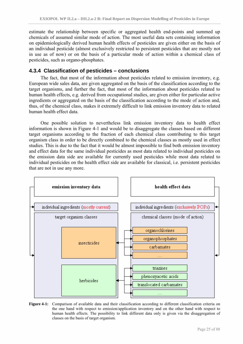
Figure 4-1: Comparison of available data and their classification according to different classification criteria on the one hand with respect to emission/application inventory and on the other hand with respect to human health effects. The possibility to link different data only is given via the disaggregation of classes on the basis of target organism...............................25
Figure 5-1: Conceptual structure of a full chain assessment of pesticides following the Impact Pathway Approach by starting from the use/application of pesticides resulting in emissions/releases into the environment, the fate behaviour and exposure of pesticides as well as the monetary valuation of related welfare losses. Each step of the pathway shows involved media and processes or pathways, respectively. *formation of non-extractable residues. **denotes that for food ingestion not only field crops but also animals, e.g. cattle, are taken into account. .............................................................................................................................35
Figure 5-2: Flow scheme for the calculation/estimation of pesticides emissions to air by selecting an approach on the basis of data availability. The numbers denote the chronological order of assessing availability of data and calculating emissions from these data, respectively (adapted from European Environment Agency, 2007).............................................................37
Figure Annex 1: World map of global gridded alpha-HCH emissions [treleased/yr/cell] for 1990 with 1° latitude by 1° longitude grid resolution (Environment Canada and Global Emissions Inventory Activities working group, GEIA). ...........................................................................68
Figure Annex 2: γ-HCH emissions in the northern hemisphere and European region for the period from 1990 to 2004 (Meteorological Synthesizing Centre-East, MSC-East).................69
Figure Annex 3: Aggregated emissions of Hexachlorocyclohexane to air and direct to water per industrial activity in which the emissions are generated in EU25 in 2004 (European Pollutant Emission Register, EPER). .......................................................................................70
EXIOPOL WP II.2.a – DII.2.a-2 B: Final Report on Dispersion Modelling of Pesticides in Europe
Page 8 of 88
1 Aim and structure The present paper aims at giving an overview of how to conceptually develop and adapt
the impact-pathway methodology to the impact chain of pesticides. On the basis of this paper the development and implementation of a modelling framework is in progress that in the end should be used to conduct a full chain assessment of pesticides for estimating impacts to human health and related external costs from the amount released into the environment by means of different case studies within the geographical scope of Europe. This is in line with the overall objective of EXIOPOL, which is to synthesise and develop a methodological and modelling framework for allowing a consistent estimation of environmental impacts and external costs of different economic sector activities, including agricultural practices of widely using plant protection products3. Environmental impacts within the frame of EXIOPOL, however, are restricted to human health impacts, although impacts on ecosystems due to application of plant protection products also play a significant role as part of the overall environmental burdens (Schäfer et al., 2007; Liess et al., 2005; Liess & Schulz, 1999). Furthermore, in this project the human health impacts due to pesticide use are generally related to intake via ingestion of different food items as the pesticide intake via ingestion of drinking water as well as via inhalation is around 5-9 orders of magnitude lower and, thus, negligible compared to intake via ingestion of food (Juraske et al., 2007a, 2007b; Lu et al., 2008). Out of the set of different economic sector activities only agriculture is taken into account in this work package as it is estimated that more than 99 percent of the total pesticide emissions in Europe originate from agricultural use (European Environment Agency, 2007).
Findings of this paper should help to bridge relevant gaps between different parts of a full
chain pesticide assessment by revealing mismatches of required data as well as by bringing together knowledge of how to set up a full chain modelling approach with a consistent data-set in as complete a way as possible. In doing so, the present document follows a structure which is in line with the methodology of a general full chain assessment as described in Bickel & Friedrich (2005) and in European Commission (2003) by starting at the definition and estimation of the source strength, hereafter referred to as either emission or release of pesticides (cf. Section 5.1), following the pathway of the chemicals through the different environmental media involved up to the considered receptors, hereafter referred to as their environmental fate (cf. Section 5.1.1), further following the different exposure pathways (cf. Section 5.3) and the relationships of those to human health effects, hereafter referred to as human health impacts (cf. Section 5.4) and finally the monetary valuation of the calculated effects (cf. Section 5.5). Beforehand, the present paper will deal with some definitions and considerations of technical terms and methodologies for assessing pesticide externalities as well as with temporal and spatial aspects regarding the full chain approach (cf. Chapter 3). In addition, the problem of classifying pesticides on the basis of the data availability with respect to emission and effect information is discussed in Section 4.3 in order not to calculate several hundreds of chemicals for which such data are only rarely, if at all, available. Finally, some information about how to apply the developed methodology in a respective modelling framework will be given in Chapter 6.
3 The difference between the terms ‚pesticide’ and ‚plant protection product’ is discussed in detail in Section 3.1.

EXIOPOL WP II.2.a – DII.2.a-2 B: Final Report on Dispersion Modelling of Pesticides in Europe
Page 9 of 88
2 Background At the EXIOPOL WSII.2 meeting in Aarhus at April 7th 2008, in which partners from
NERI, NIVA and USTUTT attended and IOM participated some of the time by video conference, the need was identified to have an overview note addressing some methodological issues about how, within EXIOPOL, we will estimate the public health effects of the use of pesticides in the EU. Such a note was offered by IOM and serves as basis for the human health impact assessment of the present document as described in Section 5.4.
In addition, also for the part of the full chain approach that focuses on the estimation of
emissions at the European scale it was agreed that a further analysis and definition of the pathway of pesticides is required. That is, the impact pathway generally starts with direct emissions into the medium air and/or direct and indirect releases into the media water and soil, but in order to meet the requirements of the Input-Output Methodology (I/O) used throughout the EXIOPOL project the approach must also account for the application of pesticides. Thus, the steps to be additionally considered and implemented in the full chain methodology are as follows:
• From pesticides sales and/or supply (consumption data) to application of pesticides (optional, i.e. only if no application data are available), and
• From application of pesticides (use) to pesticide emissions/releases into the environment (mandatory).
A detailed description of how to address the additional steps in the full chain approach is presented in Chapter 5. More information about the I/O Methodology in general and the requirements for a proper application of Supply and Use Tables (SUT) and Input-Output Tables (IOT) are to be found in Deliverable DIII.1.a-5 (Technical Report: Definition Study for the EE IO Database)4.
During the EXIOPOL WSII.2 meeting the most important gap that the work stream partners have found to be addressed with respect to the full chain approach, however, is to link the application or emission data to epidemiologically derived effect information as both have a basis regarding the pollutants and/or pollutant classification that may not be consistent for performing cross-cutting issues, such as to conduct a full chain approach from pesticide application to human health effect estimations. It has thus been agreed that USTUTT and IOM discuss the discrepancies between the emission and the effect data sets and based on that work out a classification of pesticides for application in the context of a full chain assessment by setting up a respective paper. This conceptual paper will additionally be used to define the format of the required pesticide emission and effect information within the frame of an externality assessment in EXIOPOL. The further outcome of this conceptual paper is a selection of prioritised pesticides and/or pesticide classes for which a full chain externality assessment will be conducted by means of at least one case study as further described in Chapter 6.
4 http://www.feem-project.net/exiopol/userfiles/EXIOPOL_DIII_1_a_5_final(1).pdf
EXIOPOL WP II.2.a – DII.2.a-2 B: Final Report on Dispersion Modelling of Pesticides in Europe
Page 10 of 88
3 Definitions and considerations of relevant terms
3.1 Nomenclature of substances of concern In the widest context, environmental chemicals are sometimes also referred to as ‘man-
made substances’ (Bachmann, 2006), but can in fact either be defined as chemicals that naturally occur in the environment or as chemicals which enter the environment as a result of human activity, such as agricultural practice. Independently from their source, such chemicals occur in concentrations in the environment that may put living organisms, particularly human beings, to a risk (e.g. Bliefert, 2002). However, within the context of the present document only environmental chemicals related to the agricultural sector are of concern, in particular chemicals that protect and promote a selected field and/or horticultural crop, so-called plant protection products.
According to Article 2 of the Council Directive 91/414/EEC of the European Commission5
a plant protection product is an ‘active substance and preparation containing one or more active substances, put up in the form in which it is supplied to the user, intended to:
• Protect plants or plant products against all harmful organisms or prevent the action of such organisms, in so far as such substances or preparations are not otherwise defined below;
• Influence the life processes of plants, other than as a nutrient, (e.g. growth regulators); • Preserve plant products, in so far as such substances or products are not subject to
special Council of Commission provisions on preservatives; • Destroy undesired plants; or • Destroy parts of plants, check or prevent undesired growth of plants.
According to its definition, the main purpose of a plant protection product is to protect plants and plant products against organisms harmful to plants and plant products. When these products are directly applied on plants and plant products it is clear that the purpose is according to the definition and therefore they are clearly plant protection products. This applies in every place where these products are used, both inside and outside the farm, for example in stores of plant products. In the cases where products are used for a general hygiene purpose (normally not directly applied to protect plants or plant products) or when it is not clear which kind of products will be stored after the treatment it is agreed to consider these products generally as biocidal products.
In order to distinguish between plant protection products and biocidal products, there exist a guidance document that was agreed between the Commission services and the competent authorities of Member States on the borderline between Directive 98/8/EC concerning the placing on the market of Biocidal products and Directive 91/414/EEC concerning the placing on the market of plant protection products6. According to Article 2 of the Council Directive 98/8/EC of the European Commission7, a biocidal product is an ‘active substance and preparation containing one or more active substances, put up in the form in which it is supplied to the user, intended to destroy, deter, render harmless, prevent the action of, or otherwise exerts a controlling effect on any harmful organism by chemical or biological means.’
5 http://ec.europa.eu/food/plant/protection/index_en.htm 6 http://ec.europa.eu/food/plant/protection/evaluation/borderline_en.htm 7 http://ec.europa.eu/environment/biocides/index.htm

EXIOPOL WP II.2.a – DII.2.a-2 B: Final Report on Dispersion Modelling of Pesticides in Europe
Page 11 of 88
In contrast to the terms plant protection product and biocidal product the term pesticide will be finally used throughout work stream WSII.2 and thus also in the present document. As further explained in Section 4.3, pesticides can be subdivided into classes according to the target organism that is intended to be controlled by the use of a pesticide. Amongst others, insecticides and herbicides are such subdivision classes. According to the definition of plant protection products, insecticides and herbicides are clearly within the scope of Directive 91/414/EEC, as long as they are clearly used to protect plants, as described above. A pesticide, however, only corresponds to the subgroup of plant protection products that are clearly intended to protect plants from harmful organisms as well as to destroy undesired plants or parts of plants. Consequently, pesticides are hereafter referred to as a subgroup of plant protection products with specific intentions of usage and out of these will only focus on the protection against harmful and/or undesired insects and plants, i.e. insecticides and herbicides, and will be used throughout the present document to describe the active ingredient that is mainly defining the intention of usage.
Pesticides, however, may be further classified according to various options, such as their
physico-chemical properties, chemical structure, application, toxicity. Within the frame of EXIOPOL, the term ‘pesticides’ can basically be further subdivided into classes on the basis of a chemical’s application: acaricides, algaecides, arboricides, avicides, bactericides, fungicides, herbicides, insecticides, molluscicides, nematicides, rodenticides or virucides. Out of these classes only insecticides and herbicides should be taken into consideration for the tasks within WS II.2, which is in accordance with the project’s DoW. How the term ‘pesticide’ is to be further defined with respect to different sources, i.e. natural and anthropogenic, will be outlined in Section 3.4 in the context of the spatial resolution of pesticide emission sources.
3.2 Considerations with respect to Health Impact Assessment In recent years, Health impact assessment (HIA) has emerged as an important means of
promoting healthy public policy (Petticrew et al., 2007). HIA developed from a concern that major social interventions, such as environmental policies, could have negative health effects and that the consideration of human health effects played a too limited role so far, e.g. in Environmental Impact Assessment (ibid.).
The importance of HIA has been emphasised in successive EU and WHO policy
documents, statements and recommendations and, although the range of activities described as HIA is broad, it is usually defined, according to what is known as the Gothenburg Consensus Paper (European Centre for Health Policy, 1999), as “a combination of procedures, methods and tools by which a policy, programme or project may be judged as to its potential effects on the health of a population, and the distribution of those effects within a population”. A key word here is potential – HIA is concerned with estimating or predicting the health effects of policies and programmes in advance of their implementation. Thus, Kemm & Parry (2004) and Kemm (2007) identify the two essential features of HIA as follows:
• “It is intended to support decision-making in choosing between options. • It does this by predicting the future consequences of implementing the different options”
[emphasis added]. Kemm (2007) goes on to distinguish between HIA and other public health activities, including:
• Evaluation: the “systematic study of the effect of an intervention (or unplanned event such as a pollution incident)” and
• Monitoring and surveillance: the “systematic collection of information on aspects of a community’s health in order to identify emerging health problems (or benefits)”.

EXIOPOL WP II.2.a – DII.2.a-2 B: Final Report on Dispersion Modelling of Pesticides in Europe
Page 12 of 88
Note that both evaluation and surveillance involve gathering new empirical data. For evaluation, this is as part of research to identify differences before and after an intervention and to see to what extent these differences may be attributable to the intervention (rather than to other factors which happened over the same time-period). Surveillance is focused rather on gathering new routine data, from which to identify trends and, where practicable, understand the reasons for them. In contrast to evaluation and surveillance, the major steps in conducting an HIA include:
• Screening (identify projects or policies for which an HIA would be useful), • Scoping (identify which health effects to consider), • Assessing risks and benefits (identify which people may be affected and how they may
be affected), • Developing recommendations (suggest changes to proposal to promote positive or
mitigate adverse health effects), • Reporting (present the results to decision-makers), and • Evaluating (determine the affect of the HIA on the decision process). The predictive aspect of HIA is one of its defining characteristics (Parry & Kemm, 2004).
However, the validity of those predictions remains something of an open question due to the fact that it has been suggested that the criterion of predictive validity has limited applicability, as it is not possible to follow up very long-term consequences, and it is not possible to verify the counterfactual, that is, it is not possible to check the accuracy of predictions for options that were not chosen (Kemm & Parry, 2004).
Besides the differentiation between HIA and other public health activities as well as the
predictive aspect of HIA, Kemm (2007) identifies a third characteristic which some practitioners and commentators consider to be essential: “stakeholder participation, involving the people affected by, and or who have an interest in, the decision”. In Kemm’s view this is an important aspect, but is not intrinsic.
Overall, the aim of health impact assessment is to allow a systematic consideration of
likely outcomes regarding the health of a population to be incorporated into decision-making. Obviously, the scale of any proposed plan can influence its likely effect on health, and therefore involves the need for a full health impact assessment, e.g. by applying a full chain approach, such as the Impact Pathway Approach as described in the following section.
3.3 Impact Pathway Approach The Impact Pathway Approach (IPA) has been developed within the series of ExternE
Projects on ‘External Costs of Energy’ funded by the European Commission (Bickel & Friedrich, 2005). It is a bottom-up approach in which the causal relationships from the release of contaminants through their interactions with the environment to a physical measure of impact (the ‘impact pathway’) and, where possible, a monetary valuation of the resulting welfare losses is assessed (see Figure 3-1).
As it was the objective of the ExternE studies to achieve an economic valuation of impacts,
the impact assessment procedure that has been implemented into related modelling frameworks based on the IPA so far is very much oriented to arrive at the damage level. Due to the modularity of the IPA, results can be provided on various intermediate levels of the environmental mechanism and, in addition, it can be used independently of any valuation methodology. According to its being a bottom-up approach, the IPA strives for a high spatial resolution in order to capture the sources of the substances, i.e. human activities. Unlike

EXIOPOL WP II.2.a – DII.2.a-2 B: Final Report on Dispersion Modelling of Pesticides in Europe
Page 13 of 88
regulatory risk assessments, the impacts or rather the ‘risks of impacts to occur’ that are assessed by the IPA are intended to be representative (so-called central or best estimates) rather than conservative or protective (Bachmann, 2006).
Figure 3-1: Flowchart of the Impact Pathway Approach including monetary valuation. The IPA allows for
monetary valuation of impacts of chemicals on receptors by considering causalities between different stages of the chain.
The Impact Pathway Approach can be regarded as a particular example of Life Cycle Analysis (LCA) which is why in the following many concepts from this field of research are drawn from. Within the frame of work stream WSII.2 of the EXIOPOL project, the IPA will be specifically adjusted to fully assess the impact pathway of selected pesticides and/or pesticide classes as further described in Section 4.3. Some parts and/or causalities between the stages of the IPA, hence, were added or modified to extend the IPA methodology to also consider the physico-chemical properties and the fate and exposure behaviour of pesticides, in particular insecticides and herbicides. How and to what extent the IPA methodology has been modified and applied within the frame of EXIOPOL is described in detail in Chapter 5.
3.4 Spatial and temporal aspects of the present approach The whole impact assessment is to be performed in a spatially-resolved way. Principally
one may distinguish site-generic from site-dependent and site-specific assessments (cf. Hauschild & Potting, 2003). In site-generic assessments, all sources are considered to contribute to the same generic receiving environment while a moderate to high degree of spatial differentiation in terms of emission sources and/or receiving environment is employed for site-dependent and site-generic approaches, respectively. In order to allow for a site-dependent and/or site-specific assessment, a comprehensive set of relevant input data for the whole of Europe is required, i.e. information of application and emissions of pesticides. In order to conduct consistent and comprehensive application and emission estimations as data basis for a full chain modelling assessment, it is necessary to identify whether and between what spatial and temporal scales it will be required to aggregate or disaggregate existing data. This is, e.g. due to the fact that “different processes and connectivities emerge as dominant as we move from the plot scale to catchment or regional scales” (Kirkby et al., 1996, p. 396). Thus, the way how a chemical of concern enters the environment as well as the source type of this chemical are of particular interest and will be discussed in the following with respect to spatial and temporal aspects.

EXIOPOL WP II.2.a – DII.2.a-2 B: Final Report on Dispersion Modelling of Pesticides in Europe
Page 14 of 88
First of all, it is to be defined whether the chemical category of pesticides either comprises
anthropogenic sources, i.e. releases from various human activities, such as industrial processes, natural sources, i.e. processes occurring in vegetation and soils, in marine ecosystems, as a result of geological activity in the form of geysers or volcanoes, as a result of meteorological activity such as lightning, and from fauna, such as ruminants and termites, or both source categories. This question requires a further clarification of how the term ‘pesticide’ is defined within the scope of the EXIOPOL project. In line with, e.g. the European Environment Agency and the United States – Environmental Protection Agency, a pesticide is defined as substance or mixture thereof intended for (i) preventing, destroying, repelling, or mitigating any pest or (ii) for use as a plant regulator, defoliant, or desiccant. A pesticide in which the active ingredient is a biochemical or some other naturally-occurring substance, is referred to be a ‘natural pesticide’, while it is called a ‘synthetic pesticide’ when its active ingredient has been manufactured. Examples for natural pesticides are pyrethrin which is extracted from specific chrysanthemum species (Chrysanthemum spec.) or azadirachtin, an extract from the neem tree (Azadirachta indica). Both are widely used as insecticides for, e.g. inhibiting the development of larvae of various insects.
However, independently from the origin of its active ingredient, a pesticide unexceptionally is applied by humans, so that the category ‘natural sources’ is assumed not to be relevant for the estimation of pesticide emissions. According to the Emission Inventory Improvement Program of the United States – Environmental Protection Agency (United States – Environmental Protection Agency, 2001) and the Atmospheric Emission Inventory Guidebook of the European Commission (European Environment Agency, 2007) emission sources in general are further distinguished according to their spatial extension as follows:
• Point sources: large, stationary, identifiable sources of emissions that release pollutants into the atmosphere. Point sources are typically large manufacturing or production plants. They typically include both confined ‘stack’ emission points as well as individual unconfined ‘fugitive’ emission sources. Within a given point source, there may be several ‘emission points’ that make up the point source. This term should not be confused with point source, which is the regulatory distinction from area and mobile/line sources. The characterization of point sources into multiple emissions points is useful for allowing more detailed reporting of emissions information.
• Area sources: smaller sources that do not qualify as point sources under the relevant emissions cut-offs. Area sources encompass more widespread sources that may be abundant but that, individually, release small amounts of a given pollutant. These are sources for which emissions are estimated as a group rather than individually. Examples typically include dry cleaners, residential wood heating, auto body painting, and consumer solvent use.
• Mobile sources/line sources: include all non-stationary sources, such as automobiles, trucks, aircraft, trains, construction and farm equipment, and others, except sources within an urban area as these belong to area sources (European Environment Agency, 2007). Mobile sources, however, are a subcategory of area sources.
By following this classification of emission sources, mobile sources can be excluded from the list of pesticide emission source categories as pesticide use is restricted to agricultural fields and private and urban gardens and parks, all of which are stationary. While agricultural fields can beyond question be allocated to the category ‘area sources’, the assignment of private and urban gardens and parks primarily depends on their spatial extension, why it is useful to take the geographical scope of the project into account for a proper source assignment, and that is the
EXIOPOL WP II.2.a – DII.2.a-2 B: Final Report on Dispersion Modelling of Pesticides in Europe
Page 15 of 88
whole of Europe. An assessment which is European-wide rather shows spatial resolutions of some ten kilometres or even lower (Potting & Hauschild, 2005; Janssen et al., 1999), be it as a sub-division into a regular grids (e.g. polar-stereographic), as a sub-division into catchments or administrative units. Hence, for urban parks as well as for all kinds of gardens it is suitable to be also assigned to the ‘area source’ category.
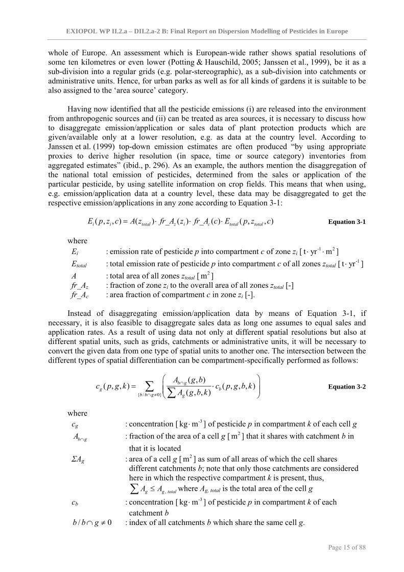
Having now identified that all the pesticide emissions (i) are released into the environment
from anthropogenic sources and (ii) can be treated as area sources, it is necessary to discuss how to disaggregate emission/application or sales data of plant protection products which are given/available only at a lower resolution, e.g. as data at the country level. According to Janssen et al. (1999) top-down emission estimates are often produced “by using appropriate proxies to derive higher resolution (in space, time or source category) inventories from aggregated estimates” (ibid., p. 296). As an example, the authors mention the disaggregation of the national total emission of pesticides, determined from the sales or application of the particular pesticide, by using satellite information on crop fields. This means that when using, e.g. emission/application data at a country level, these data may be disaggregated to get the respective emission/applications in any zone according to Equation 3-1:
( , , ) ( ) _ ( ) _ ( ) ( , , )i i total z i c total totalE p z c A z fr A z fr A c E p z c= ⋅ ⋅ ⋅ Equation 3-1
where Ei : emission rate of pesticide p into compartment c of zone zi [ -1 2t yr m⋅ ⋅ ] Etotal : total emission rate of pesticide p into compartment c of all zones ztotal [ -1t yr⋅ ] A : total area of all zones ztotal [ 2m ] fr_Az : fraction of zone zi to the overall area of all zones ztotal [-] fr_Ac : area fraction of compartment c in zone zi [-].
Instead of disaggregating emission/application data by means of Equation 3-1, if
necessary, it is also feasible to disaggregate sales data as long one assumes to equal sales and application rates. As a result of using data not only at different spatial resolutions but also at different spatial units, such as grids, catchments or administrative units, it will be necessary to convert the given data from one type of spatial units to another one. The intersection between the different types of spatial differentiation can be compartment-specifically performed as follows:
{ / 0}
( , )( , , ) ( , , , )
( , , )b g
g bb b g g
A g bc p g k c p g b k
A g b k∩
∩ ≠
⎛ ⎞= ⋅⎜ ⎟⎜ ⎟
⎝ ⎠∑ ∑
Equation 3-2
where cg : concentration [ -3kg m⋅ ] of pesticide p in compartment k of each cell g
b gA ∩ : fraction of the area of a cell g [ 2m ] that it shares with catchment b in that it is located
ΣAg : area of a cell g [ 2m ] as sum of all areas of which the cell shares different catchments b; note that only those catchments are considered here in which the respective compartment k is present, thus,
, g g totalA A≤∑ where Ag, total is the total area of the cell g
cb : concentration [ -3kg m⋅ ] of pesticide p in compartment k of each catchment b
/ 0b b g∩ ≠ : index of all catchments b which share the same cell g.

EXIOPOL WP II.2.a – DII.2.a-2 B: Final Report on Dispersion Modelling of Pesticides in Europe
Page 16 of 88
Equation 3-2 can easily be adapted to also translate data the other way round, i.e. from grid to catchment differentiation, as well as between other spatial unit types, e.g. administrative units, by replacing just the respective units in the formulation. More information about the spatial resolution of available application and/or sales data is to be found in Section 5.1.
After discussing the spatial aspects of the application of pesticides the temporal characteristics are to be discussed in the following as they are likely to be significant as well for a full chain assessment. In particular, this means that dynamic or episodic models may require emission inputs with a time resolution of the order of an hour while long term models basically use seasonal or annual average emission input data (Scholtz et al., 1999). Although most results of such modelling approaches underline the importance of seasonal pattern of pesticide application (see Figure 3-2), data availability is critical not only in space but also in time when trying to cover a rather larger geographical area with some degree of spatial resolution.
Figure 3-2: Comparison of the predicted weekly emission factors due to tilling soil with residues of α-hexachlorocyclohexane from the previous year’s planting of treated seed and emissions due to current year’s post-emergent spray application (from Scholtz et al., 1999).
For geochemical processes, as an example, Drever notes that “it is rarely possible to
construct a meaningful catchment budget for a time-scale of less than a year (Drever, 1997, p. 241). Hence, the full chain approach of pesticides for the whole of Europe to be conducted within the frame of EXIOPOL shall be based on annual average data for pesticide emissions/applications and/or production or sales data. How this data resolution will affect the overall modelling approach is further discussed in Sections 5.1 and 5.1.1.
Regarding the timeliness of data dissemination it was agreed that the full EXIOPOL EE-IO
database will be developed for the base year 2000, with an extrapolation to the year 2005 on the basis of an analysis of the health effects of baseline and change scenarios that will focus on the effects of emissions in the EU in selected recent or future years. This opens questions about the future of EXIOPOL after project closure, about foreseeable extensions and updates, about the protocols for maintenance and their cost, as mentioned in Deliverable D I.1.A-1 (Concise report with expectations of the outcome of this project from policy circles, and implications fro Cluster
EXIOPOL WP II.2.a – DII.2.a-2 B: Final Report on Dispersion Modelling of Pesticides in Europe
Page 17 of 88
II and III)8. The research team takes into account from the start the possibility to update the data in order to generate trends. However, for the estimation of externalities of pesticide application in Europe it would be far beyond the scope of the work of WSII.2 to also include the time farer in the future, such as the year 2020. This is due to the fact that it is highly uncertain to predict which active ingredients will be used in, e.g. 2020 throughout Europe according to the trend of frequently adjusting the authorised pesticides in the Regulation 91/414/EEC of the European Commission – it was last updated in September 2007 for Trifluralin, Benfuracarb and 1,3-Dichloropropene 9.
Finally, the problem of time delays in the full chain approach has to be taken into consideration as changes in risks to health may not be immediate. They may be delayed because:
(i) There is a time-lag between emission and exposure and/or (ii) There is a time-lag between exposure and health effect.
EXIOPOL will thus aim to estimate attributable effects on human health, whether these health effects occur soon after emissions or are delayed. In addition, EXIOPOL will aim to estimate the distribution of the length of time post-emissions when attributable health effects occur.
8 http://www.feem-project.net/exiopol/userfiles/EXIOPOL_DI_1_a_1_final.pdf 9 Decisions and review reports as of early October 2008: http://ec.europa.eu/food/plant/protection/evaluation/

EXIOPOL WP II.2.a – DII.2.a-2 B: Final Report on Dispersion Modelling of Pesticides in Europe
Page 18 of 88
4 Framework and objective of estimating pesticides externalities in EXIOPOL
4.1 Conceptual framework With more than 10 000 commercial formulations of several hundred active ingredients
currently on the market pesticides are widely used in agricultural practice all around the world (Alloway & Ayres, 1997). The usage of pesticides and thus their dispersion and fate in the environment has mainly occurred in the last 6 decades and they have become relatively ubiquitous pollutants, especially in technologically advanced countries, such as the U.S. and most countries of the EU. Hence, pesticides can be found in human as well as in animal tissues, in different agricultural soils and adjacent areas, in groundwater, in rivers and lakes and in various items of the food chain (Arias-Estévez et al., 2008; Hamilton & Crossley, 2004; Juraske, 2007; Margni et al., 2002). However, the transport of pesticides in the atmosphere, in the oceans and in the marine food chain has resulted in their wider global distribution. Hence, concentrations of several pesticides can even be also found in the Arctic snows (Herbert et al., 2005), in Antarctic penguins (Geisz, 2008) and last but not least in the atmosphere all over the world including the polar regions (Li & Macdonald, 2005; Hung et al., 2002).
EXIOPOL as an international and integrated project appropriately addresses the
transnational aspects as well as the most important exposure pathways for pesticides which allows for an assessment in an as comprehensive a way as possible. An example of transnational aspects is long-range transport as a component of the environmental fate of a pesticide that is one part of the transportation processes that lead to its global distribution.
The main aim of the EXIOPOL project is to create a monetary input-output table with
environmental extensions including externalities resulting from agricultural activities. This input-output table will cover around 130 industrial sectors and products in the 27 Member States of the EU as well as in 16 non-EU countries, such as the U.S., China, or Brazil. The data collected will be based on national supply and use tables which will be linked using trade date for all the countries included in the analysis. Due to this large amount of data requirements, there are a number of criteria that have to be fulfilled to allow for and facilitate the integration of the externalities of different agricultural practices, with pesticides being a major part of the work in this field of research.
First of all, within work package WPII.2.a of Cluster II of this project, the collection of
data on pesticide application and emissions was agreed to be the starting point for the externality assessment of the agricultural sector, while the results of the whole externality assessment serve as input for the input-output table to be implemented in Cluster III. This is in line with the fact that according to the Description of Work of EXIOPOL the partners of work stream WSII.2 are responsible for the externality estimation with respect to agriculture (WSII.2: Externalities of different types of agricultural practice and introduction of new practice (excluding biodiversity)), while Cluster III has as main goal to develop an operational and detailed EU-25 input-output table with environmental extensions. This input-output table is basically an economic input-output table to which per sector discerned information about emissions and resource use is added. The database that, in relation to this, is to be developed, will include external costs per sector as calculated in Cluster II, e.g. for the application of pesticides. The input-output table will be based on data for the year 2000 and will be extrapolated into the year 2005. Thus, data used for the quantification of, e.g. pesticide emissions and modelling their

EXIOPOL WP II.2.a – DII.2.a-2 B: Final Report on Dispersion Modelling of Pesticides in Europe
Page 19 of 88
behaviour in the environment and receptors of concern will also be calculated for the same years, i.e. 2000 and 2005 as described in detail in Section 3.4. With respect to be able to compare future effects and damages with current ones – by weighting the former less than the latter by means of discounting (cf. Section 5.5) – it has been proposed to deliver a range of substance-specific external cost values. While this range of values will account for different discounting assumptions it should, in addition, also derive a mean value, which is defined as the value with the highest probability out of the range of values and will serve as central value for the calculations of the externality estimations. Furthermore, the resulting external costs will be categorised into ‘impacts on human health’, ‘impacts on ecosystems’ and ‘impacts on climate change’. As regards the spatial resolution, data, such as pesticide sales or application information, are required at least at the national level (cf. Section 3.4). These data could directly be included into the national supply and use tables and will be aggregated on a European-wide level in a later step. Finally, data of pesticides emissions into the environment are to be provided in [kg/year] or [t/year], as external cost values will be generally calculated either in [Euro/kg/year] or [Euro/t/year] when they are given as incremental damages or in [Euro/kg] or [Euro/t] when they are given as accumulated damages.
In addition to the application of the results of this work stream for the estimation of
external cost due to the usage of pesticides in agricultural practices as well as the inclusion of the results in the final extended input-output table in Cluster III of this project, the information gathered will also be applied in Cluster IV. This cluster focuses on the implications for policy which are to be extracted from the findings of the externality research including agricultural externalities. Therefore, the environmental burden of activities in the agricultural sector will be analysed in different future scenarios and then linked to the use of different agricultural subsidies at the national and/or European scale.
In order to interlink the different aspects concerning policy, economy and the environment
including human health, the full chain from policy to external costs must be taken into consideration. Although the full chain approach is much too limited and simplistic to encompass the full complexity of relationships between environmental policies, the environment, and human health, it provides a framework for working through the policies that affect environmental chemicals and physical stressors, and, through these, affect environmental and human health. However, as also mentioned in other projects, such as HEIMTSA, the full chain approach is the methodological framework that is preferred by the European Commission, and which through its name of being an ‘Impact Pathway Approach’ many of the partners are familiar with, who are involved in the EXIOPOL project. Within EXIOPOL, the general methodology of the full chain approach is used for assessing externalities of different economic sectors and will be adopted as well for the externality assessment of pesticides released into the environment by agricultural practice. In general, the full chain approach chronologically follows the pathway of a chemical through the stages of the chain as follows:
• From (changes in) policy; to • (changes in) emissions to air and/or releases into soil and water; to • (changes in) concentrations in environmental media (including micro-environments); to • (changes in) exposures of targeted receptors (e.g. humans: exposure of individuals and
populations via inhalation, dermal and/or ingestion routes; to • (changes in) internal dose at target organs (e.g. lung, liver) in the receptors; to • (changes in) risks of (human) health effects; to • (changes in) health impacts (‘annual number of incidences’) overall and in sub-
populations (e.g. children, other groups of specific vulnerability); to • (changes in) monetary value of health impacts.

EXIOPOL WP II.2.a – DII.2.a-2 B: Final Report on Dispersion Modelling of Pesticides in Europe
Page 20 of 88
Note that actions and policies can change population-attributable health effects not only by directly aiming at a change in emissions or releases of a chemical but also by acting at various other stages of the chain. For example, and in particular, exposure is determined not only by emissions and usage, with consequences for the concentrations of pesticides in various (micro-) environments. It is also determined by the characteristics and habits of the population at risk. Actions to limit exposure may focus on usage and, thus, on concentrations in (micro-) environments. On the other hand, actions may also focus on, e.g. informing the population so that the total population-weighted exposure is reduced.
The general full chain approach was adapted to meet the specific requirements of an externality assessment of pesticides at the European scale and follows the methodological concept of the Impact Pathway Approach, according to its definition in Section 3.3 and its application for a site-specific assessment of pesticides in Chapter 5. How the development and application of the presented methodology will be integrated into the overall objective of the EXIOPOL project is subject of the following section.
4.2 Objective of estimating externalities of pesticide usage The general methodological issues in the present document as part of the overall objective
of the EXIOPOL project are strongly based on corresponding and parallel developments within the project HEIMTSA; and these in turn draw on:
(i) The long-standing experience of several HEIMTSA team members in EU projects such as ExternE; and on
(ii) Methodological discussion with the INTARESE project. This has the advantage of maintaining methodological coherence between these projects. In particular, aspects of the present document draw heavily on a corresponding methodological note that, within HEIMTSA, is Deliverable 7.1.2 (Clarifying the overall conceptual framework – the scope, scale and methodology of HEIMTSA). This deliverable will in turn help with finding efficiencies in the conduct of these projects and, in addition, developing an integrated set of tools and methodologies for future use in Europe.
The objective of estimating public health effects of pesticides in this part of EXIOPOL means to estimate the public health effects associated with:
(i) Baseline conditions, i.e. current use of pesticides or predicted future use, under a scenario whereby current regulations and/or methods for limiting exposures are implemented, but new regulations and/or methods for limiting exposure are not;
(ii) Changes in exposure as a result of some new (policy) actions that ultimately affect exposure.
As already stated above, the estimated externalities derived from the estimations of public health effects will be expressed in monetary terms in order to extend the input-output framework by also including environmental factors. The estimation of external costs resulting from the use of pesticides in current and future agricultural practices is especially relevant for the comparison of these costs to the benefits of food supply and the prevention of crop losses. Thus, the externality estimations provided by this work stream will enable a sector-specific cost-benefit analysis (CBA). Additionally, a comparison of the results to the results for all other around 130 economic sectors in terms of impacts on human health, ecosystems and climate change, will become possible. Last but not least, the results will be included in the work of Cluster IV where the evaluated environmental burdens of agricultural activities will be used to analyse implications for policy actions related to agricultural subsidies.
In order to work out all the characteristics and processes to be considered for a substance-specific (or substance class-specific) estimation of externalities due to the application of
EXIOPOL WP II.2.a – DII.2.a-2 B: Final Report on Dispersion Modelling of Pesticides in Europe
Page 21 of 88
pesticides in agriculture, it is as a first step necessary to define the selection of substances of concern for the whole assessment. This will be done in the following section.
4.3 Selected pesticides or pesticide classes for a full chain assessment As mentioned above, pesticides may be further subdivided into classes according to
different parameters, such as the target organism that is intended to be controlled by the use of a pesticide. It will be further discussed in the following sections why insecticides and herbicides are subdivision classes, out of which, within this work stream of the EXIOPOL project, some single active ingredients and/or types of active ingredients will be investigated by means of a full chain approach. In addition to the classification of pesticides due to data availability reasons, one more question has been raised at the last work stream meeting in 2008: “Which pesticides will EXIOPOL focus on in particular?” This will be discussed in the following.
According to the objective of WPII.2.a and WPII.2.c a detailed environmental fate and
exposure modelling approach of pesticides is to be developed and applied in order to link a resulting externality valuation to levels of agricultural activities in as appropriate a way as possible. Hence, as a first step the gap is to be bridged between available data of crop protection applications and respective environmental burdens. This can be realised by following the whole chain of a pesticide of concern or, if required, a mixture of pesticides, through its release into environmental media, i.e. mostly agricultural soils, its transfer and chemical transformation in the environment, to end up in receptors of interest, e.g. humans, where it potentially leads to (negative) effects that are finally to be valued by means of monetary terms.
Covering this pathway from the release of a pesticide to its concentration in environmental
media after being transported and transformed is the main focus of Task 2, which is “Emission Quantification and Dispersion Modelling of Pesticides”. Thus, the main subject of Section 5.1 aims at giving a first overview of the state of the art of data availability for pesticide emission/application data, in general at the European scale and in particular at the national scale for selected countries by reviewing publicly available inventory data-sets for pesticide application.
4.3.1 Classification of pesticides – criteria Some of the main types of active ingredients used as insecticides or herbicides or both that
are either currently in use in at least one European country or belong to the group of Persistent Organic Pollutants (POPs) due to their long degradation time in the environment are given in Table 4-1.
The fact, that these pesticides are either still in use within Europe and/or can be defined as
persistent, may be helpful for the partners of the work stream, who are involved in the process of identifying and classifying pesticides, as indicator to rank the substances according to their importance for the whole assessment.

EXIOPOL WP II.2.a – DII.2.a-2 B: Final Report on Dispersion Modelling of Pesticides in Europe
Page 22 of 88
Table 4-1: Main chemical classes of active ingredients used as insecticides or herbicides including examples that can be defined as Persistent Organic Pollutants and/or are referred to be the most important insecticides or herbicides currently in use in at least one of the Member States of the EU as of 2008.
Chemical Class Example In Use1 Perstistent2
DDT3 no yes Organochlorine y-HCH3 no yes Aldrin3 no yes Cyclodiene (Organochlorine)
Chlordane3 no yes Malathion3 yes no Organophosphate
Chlorpyrifos3,4 yes no Fenoxycarb3 yes no
Inse
ctic
ides
Carbamate Aldicarb3,4,5 yes no 2,4-D3,5,6,7 yes no Phenoxyacetic Acid
MCPA3,5,6,7 yes no Dinitroaniline Trifluralin3,5 yes yes Triazine Atrazine3,5,6,7 yes no Phenylurea Isoproturon3,5 yes no
Diquat3 yes yes Bipyridilium Paraquat3,4,5,6 no yes
Glycine Derivative Glyphosate3,5 yes no Phenoxypropionate ‚Mecoprop’3,5 yes no Translocated Carbamate Asulam Sodium3,5 yes no
Her
bici
des
Hydroxybenzo Nitrile Bromoxynil3,4 yes no 1 Reference year is 2008; refers to the application of the active ingredient in at least one of the Member States of
EU27 as of October 2008. 2 Generally belonging to the category of Persistent Organic Pollutants as declared in Annex D of the Stockholm
Convention of Persistent Organic Pollutants (POPs)10. In case an example is declared not to be persistent here, this does not mean that it is fast degrading in all involved environmental compartments, but at least has a DT50 value in soil smaller than 180 days.
3 FOOTPRINT Project (Creating tools for pesticide risk assessment and management in Europe): The FOOTPRINT Pesticide Properties Database (http://www.eu-footprint.org/ppdb.html)
4 European Commission (2007) The use of plant protection products in the European Union, data 1992-2003. Eurostat Statistical books 2007, Brussels. (http://www.eds-destatis.de/downloads/publ/en8_plant_protection.pdf)
5 Bundesamt für Verbraucherschutz und Lebensmittelsicherheit, BVL (2008) List of Authorized Plant Protection Products in Germany with Information on Terminated Authorizations. Date: July 2008.
(https://portal.bvl.bund.de/psm/servlet/HandlerSuchForm?gesamt=true) 6 Bundesamt für Verbraucherschutz und Lebensmittelsicherheit, BVL (2008) Pflanzenschutzmittel-Verzeichnis
2008 Teil 1: Ackerbau – Wiesen und Weiden – Hopfenbau – Nichtkulturland. (http://www.bvl.bund.de/cln_027/nn_492012/DE/04__Pflanzenschutzmittel/00__doks__downloads/psm__verz__2
008__1.html) 7 Bundesamt für Verbraucherschutz und Lebensmittelsicherheit, BVL (2008) Absatz an Pflanzenschutzmitteln in der
Bundesrepublik Deutschland für das Jahr 2007: Ergebnisse der Meldungen gemäß §19 Pflanzenschutzgesetz. (http://www.bvl.bund.de/cln_027/nn_492010/DE/04__Pflanzenschutzmittel/01__ZulassungWirkstoffpruefung/01_
_Aktuelles/meld__par__19__Download.html)
Another criterion for the classification of pesticides is the target organism that is intended to be controlled by the use of a pesticide. The most important classes of how pesticides are applied according to target organisms are given in Table 4-2. 10 http://chm.pops.int/Convention/tabid/54/language/en-US/Default.aspx

EXIOPOL WP II.2.a – DII.2.a-2 B: Final Report on Dispersion Modelling of Pesticides in Europe
Page 23 of 88
Table 4-2: Classification of pesticides according to the target organism that is intended to be controlled by the use of a pesticide.
Application Class Target Organism Application Class Target Organism
Acaricides Mites Herbicides Weeds Algaecides Algae Insecticides11 Insects Arboricides Groves and/or woods Molluscicides Slugs and/or snails Avicides Birds Nematicides Nematodes Bactericides Bacteria Rodenticides Rodents Fungicides Fungi and/or oomycetes Virucides Viruses
Besides the facts whether and for what target organism a pesticide is currently in use in
Europe or defined as a persistent chemical, also the data availability regarding both application and effect information should be taken into consideration. Therefore, a wide range of European-wide as well as national-wide inventory data sets have been reviewed within the frame of this work package; the results are shown in Section 5.1.2, in ‘Annex A – Pesticides application and/or emission inventory data’, in ‘Annex B – Human health effect information regarding pesticides’, and the detached document ‘MII.2.a-2_National_Pesticide_Inventories.pdf’.
How these criteria have been used to classify pesticides as to be considered within
EXIOPOL, and which pesticides and/or pesticide classes has been decides to focus on for a full chain assessment, is described in the following sections.
4.3.2 Classification of pesticides on the basis of application/emission data Amongst others, a classification of pesticides is generally possible according to the
following parameters/criteria (further explanations about the applicability of each parameter/criterion for being used to classify pesticides inventory data):
• Persistence (Most of the persistent pesticides are classical pesticides according to the definition in Chapter 5.2.2 and are either well investigated or not predominantly relevant for an assessment of currently used pesticides.);
• Current use (The number of pesticides that are currently used in different countries throughout Europe varies from country to country and is too high to be thoroughly assessed. For a complete list of pesticides currently in use including pesticides that have been banned since a couple of years already is to be found in Annex A 11.);
• Chemical class (Pesticides of different chemical classes, e.g. triazines or organophosphates, are still in use and there are no application and/or emission data sets available that distinguish their inventory data according to the chemical class of a pesticide.);
• Physico-chemical properties (As the physico-chemical properties of a pesticide determine various parameters, such as the environmental fate behaviour as well as the partitioning behaviour between the environment and the target organisms, they are implicitly considered already in other classification criteria.);
• Toxicity (Within pesticide application and emission data sets no toxicity data are considered at all, although it is one of the most important criteria for selecting a pesticide for the control of a particular target organism. However, this criterion might be
11 These can comprise Ovicides (for eggs), Larvicides (for larvae) or Adulticides (for adult insects).
EXIOPOL WP II.2.a – DII.2.a-2 B: Final Report on Dispersion Modelling of Pesticides in Europe
Page 24 of 88
helpful for a classification on the basis of available effect information as described in Section 4.3.3, but not for a classification on the basis of available emission inventory data.).
With respect to the analysed data sets dealing with application and/or emissions of
pesticides either at the European or at a national scale (cf. ‘Annex A – Pesticides application and/or emission inventory data’ and for national inventory data throughout Europe in the detached document ‘MII.2.a-2-National_Pesticide_Inventories.pdf’), the question raises which one of these criteria can be useful for a proper classification of pesticides inventory data? According to the most limiting factor, which is data availability, only one criterion or parameter will be helpful to classify pesticides with respect to inventory data, and this is the target organism that is intended to be controlled by the use of a pesticide as further defined in Section 3.1 and in Table 4-2. As most useful data sets containing information on either application, sales or emissions of pesticides are given only on the basis of a pesticides application or target organism (cf. Table 4-2), and out of these categories only insecticides and herbicides are of concern as agreed between the partners of WSII.2.
4.3.3 Classification on the basis of human health effect data Amongst others, a classification of pesticides is generally possible according to the
following parameters/criteria (further explanations about the applicability of each parameter/criterion for being used to classify pesticides health effect data):
• Persistence (Most of the persistent pesticides are classical pesticides according to the definition in Chapter 5.2.2 and are either well investigated or not predominantly relevant for an assessment of currently used pesticides. However, as most of the human health effect information are available only for chemicals out of the range of rather persistent pesticides, persistence may at least be an indicator for the investigation background of a pesticide.);
• Current use (The number of pesticides that are currently used in different countries throughout Europe varies from country to country and is too high to be thoroughly assessed. For a complete list of pesticides currently in use including pesticides that have been banned since a couple of years already is to be found in Annex A 11, although for most of the listed pesticides only rare, if at all, information with respect to human health effects are available.);
• Target organism (Pesticides can be classified according to their target organism as shown in Table 4-2, e.g. herbicides and insecticides. With respect to human health effects, however, this classification is not feasible due to the fact that these classes comprise pesticides with a wide range of physico-chemical properties and, thus, a wide range of modes of action within the human body.);
• Physico-chemical properties (As the physico-chemical properties of a pesticide determine various parameters, such as the environmental fate behaviour as well as the partitioning behaviour between the environment and the target organisms, they are implicitly considered already in other classification criteria.);
With respect to the analysed data sets dealing with human health effects of pesticides, out
of which most are related to occupational studies (i.e. epidemiologically investigated human cohorts), the question raises which one of these criteria can be useful for a proper classification of pesticides health effect data? According to the most limiting factor, which is data availability, only two criteria or parameters will be helpful to classify pesticides, and these are the toxicity, which mostly refers to a specific health end-point and makes chemicals comparable on the basis of relative toxic equivalents, and the chemical class, which, in literature, represents as a first
EXIOPOL WP II.2.a – DII.2.a-2 B: Final Report on Dispersion Modelling of Pesticides in Europe
Page 25 of 88
estimate the relationship between specific or aggregated health end-points and summed up chemicals of assumed similar mode of action. The most useful data sets containing information on epidemiologically derived human health effects of pesticides are given either on the basis of an individual pesticide (almost exclusively restricted to persistent pesticides that are mostly not in use as of now) or on the basis of a particular mode of action within a chemical class of pesticides, such as organo-phosphates.
4.3.4 Classification of pesticides – conclusions The fact, that most of the information about pesticides related to emission inventory, e.g.
European wide sales data, are given aggregated on the basis of the classification according to the target organisms, and further the fact, that most of the information about pesticides related to human health effects, e.g. derived from occupational studies, are given either for particular active ingredients or aggregated on the basis of the classification according to the mode of action and, thus, of the chemical class, makes it extremely difficult to link emission inventory data to related human health effect data.
One possible solution to nevertheless link emission inventory data to health effect
information is shown in Figure 4-1 and would be to disaggregate the classes based on different target organisms according to the fraction of each chemical class contributing to this target organism class in order to be directly combined to the chemical classes as mostly used in effect studies. This is due to the fact that it would be almost impossible to find both emission inventory and effect data for the same individual pesticides as most data related to individual pesticides on the emission data side are available for currently used pesticides while most data related to individual pesticides on the health effect side are available for classical, i.e. persistent pesticides that are not in use any more.
Figure 4-1: Comparison of available data and their classification according to different classification criteria on
the one hand with respect to emission/application inventory and on the other hand with respect to human health effects. The possibility to link different data only is given via the disaggregation of classes on the basis of target organism.

EXIOPOL WP II.2.a – DII.2.a-2 B: Final Report on Dispersion Modelling of Pesticides in Europe
Page 26 of 88
Most active ingredients of the same chemical class, such as organophosphates, are exclusively used as either insecticides or herbicides, which makes it feasible to disaggregate these classes of target organisms into chemical classes. For the cases where a chemical class is used in both, insecticides and herbicides, the fractions of the compounds used as either one are to be separated from the fractions of the compounds used as the other one. A further aspect has to be considered when applying the classes as available from effect studies with classes available from emission inventory data sets and this is the fact that the mix of pesticides of the same chemical class may vary significantly from country to country. Thus, the aggregated risk related to that chemical class, based on different modes of actions or relative toxicities of each compound of that chemical class, may vary as well from country to country.
In order to assess the feasibility of taking this approach, we have surveyed available
reviews of studies linking pesticides with health effects (Maroni and Fait, 1993; Alvanja et al, 2004; Sanborn et al, 2004; plus confidential material from an ongoing study not yet published). ‘Annex B – Human health effect information regarding pesticides’ contains a tabular summary of the conclusions drawn from these reviews, and some indications of the magnitudes of the relative risk coefficients quoted in those studies that derived them.
Interpretation of the usefulness of these results should take into consideration the following
points: • The majority of the studies reviewed were of occupational exposure to pesticides, with
some limited studies of bystander exposure, e.g. to persons living in areas where crops are sprayed.
• As noted above, it is often the case that the exposure is not characterised explicitly, and in some cases, e.g. bystander studies or studies by broad occupational category, there may be little or no information on the chemical or chemical class involved: some studies do not even distinguish between herbicides and insecticides.
• Many studies will not have had sufficient power to detect very small risks: in those cases it is to be expected that either the study would report no statistically significant effect, or would not be published at all.
• Occupational studies typically involve rather higher exposures than are to be expected in the general public. Application of available risk coefficients would therefore require considerable extrapolation to lower exposures, and that in turn would require assumptions about the shape and behaviour of the exposure-response function from the occupational exposure range to general public exposuyres. We have no information on the shape of the true function.
• It is considered that the principal route of exposure of the general public to pesticides is by ingestion. However, occupational exposures are predominantly by inhalation and by dermal absorption: we found no studies relating to ingestion exposure in humans.
• It is believed that physiologically-based pharmacokinetic (PBPK) modelling might be able to derive estimates of target organ dose from estimates of low-level ingestion exposure. However, there are no available functions for converting dose estimates to health risks.
• The above points present problems that militate against completing a full chain that links pesticide emissions with quantifiable health effects in the general population.
• Some of the health outcomes identified by the studies reviewed are cancers. A health impact assessment on cancer outcomes would need to allow for the latency of the development of cancer, whch is often taken to be 10-20 years for solid tumours and perhaps 5-10 yearsfor non-solid cancers such as leukaemia. Time to latency also affects

EXIOPOL WP II.2.a – DII.2.a-2 B: Final Report on Dispersion Modelling of Pesticides in Europe
Page 27 of 88
the relevance of studies of cancer to current conditions, since the casusative chemicals may have been out of use for some time before a study is even begun, let alone fdinsihed, published and subsequently reviewed .
An alternative solution, to be explored further in EXIOPOL, is to rely more on the assessment information that has been made available under the EU approval system for pesticides. Under Directive 91/414/EEC the more than 1.000 pesticides which were on the market prior to 1993 have been undergoing a risk assessment. Finalised in 2009, the review has resulted in the approval of about 250 substances, while the remaining either have failed or have been withdrawn from the market. The review was initially undertaken at the level of member states, but the European Food Safety Authority (EFSA) has now responsibility for the risk assessment procedure. The assessment procedure is very comprehensive and normally includes a broad risk review of the impacts on human health and ecosystem. The European Union sets Maximum Residue Levels (MRLs) for pesticide residues on food and also defines an Acceptable Daily Intake (ADI). While the MRL-value is based mainly on what is regarded as Good Agricultural Practice, the ADI-value is the estimate of the amount of food that can be ingested daily over a lifetime without appreciable health risks to the consumer. The ADI reflects chronic (long-term) toxicity. The ADI is based on the No Observed Adverse Effect Levels (NOAELs) in animal testing. A safety factor that takes into consideration the type of effect, the severity or reversibility of the effect, and the inter- and intra-species variability, is applied to the NOAEL. The NOAEL usually is divided by a safety factor of 100 to arrive at the ADI. The ADI is expressed in terms of a pesticide consumed per kilogram of body weight (mg/kg) per day. To control for the possible compliance with the ADI the member state authorities in EU calculate a Theoretical Maximum Daily Intake (TMDI), which would follow from the highest possible intake of pesticides under the guidelines. These theoretical residue calculations assume that the maximum allowable amount of a pesticide will be applied to 100 per cent of the labelled crops, that the number of pesticide applications will be in accordance with the maximum allowed by the product label, and that the food commodities will be consumed daily for a lifetime. The TMDI is calculated by multiplying the tolerance on each crop by the average daily consumption of that crop. The pesticide is believed harmless to human health where the TMDI is below the ADI. If the TMDI is above the ADI the authorities review the actual residue data or ascertain more realistic exposure estimates. These may incorporate ‘real world’ residues into calculations. Actual pesticide use, anticipated residues as determined in controlled field studies, the effects of processing, peeling, washing and cooking on residues, and regulatory monitoring data can be applied here. The real intake of pesticides is often less than one per cent of the ADI. For pesticides shown to cause cancer in laboratory animals, scientific and medical evaluations are more comprehensive. Advanced mathematical models are used to predict the impacts of a daily exposure over a 70-year period. The ultimate purpose is to predict the potential increase in cancer incidence when humans are exposed to low level residues in their diet. The ‘negligible risk standard’ suggests that the likelihood that any person will develop cancer from a lifetime exposure should be below one in a million.

EXIOPOL WP II.2.a – DII.2.a-2 B: Final Report on Dispersion Modelling of Pesticides in Europe
Page 28 of 88
Gold et. al. (1997) explored the implications for cancer rates related to pesticide residues in food by using either the theoretical maximum daily intake (TMDI) or the actual intake as calculated by food authorities. While the National Research Council had reported cancer rates generally in excess of 1/1.000.000, on basis of total diet studies estimates were a factor of 10.000-100.000 lower. Gold et. al. also provide specific cancer risk estimates for about 10 pesticides under the two different exposure measures (p. 201, table 5). For instance for the insecticide Permethrin, the cancer risk based on dietary intake is indicated to be 7,3 x 10E-7 – this insecticide accordingly provides for the highest daily intake in ug/kg per day among the 10 surveyed. While pesticide residues in food are a tightly regulated issue that should not provide for significant, unknown external costs under the new EU pesticide directive EC/396/2005, concerns remain with the exceedence of MRLs, the maximum residual levels. About five per cent of all fruits and vegetables are seen to exceed existing MRLs, many of which are still fixed by member states and not by the EU. There are also concerns with illegal use of pesticides, which seems to be more prevalent in certain member states (e.g. Spain, Poland) than in others.
4.3.5 Consideration of pesticide mixtures Aside from the identification of important pesticides to be assessed by means of a full
impact pathway approach, and the classification of pesticides on the basis of data availability with respect to application/emission and human health effect information, also the effects of pesticide mixture including the challenges in regulating such mixtures are to be considered and are, hence, discussed in the following.
Currently, methods and terminology for evaluating mixture toxicity are poorly established.
The most common approach used is the assumption of additive concentration, with the concentrations adjusted for potency to a reference toxicant (Lydy et al., 2004). Using this approach, the joint action of pesticides that have similar chemical structures and modes of toxic action can be predicted. When, e.g. on the one hand applications are given independently and at environmentally realistic concentrations, the toxicity of different pesticides varies according to their physico-chemical properties and may range from no toxicity via moderate toxicity to high toxicity. When on the other hand applying a mixture of different pesticides mimicking the composition of a commercial solution, the overall toxicity may be equal to that of the most toxic component.
However, the results of many studies show that when organisms were submitted to the real
commercial mixture containing different pesticides, solvents and additives, the toxic effects were either markedly higher than just the one of the most toxic component or the mixture shows a mode of action that is different than these of any included component (e.g. Adam et al., 2008; Hayes et al., 2006). Although in most studies it cannot be determined whether all the pesticides in the mixture contribute to the different toxicity behaviour or changing effects of the whole mixture in contrast to the single pesticides or whether some pesticides are effectors, some are enhancers, and some are neutral, many of these studies revealed that estimating human health as well ecological risks and impacts of pesticides using studies that examine only single pesticides at high concentrations may lead to gross underestimations. Particularly difficult to model are mixtures that involve a secondary pesticide that changes the toxicokinetics of a primary pesticide, which may result in increased activation or a change in the persistence of the primary pesticide within the organism, and may be responsible for a several-fold increase or decrease in toxicity (Lydy et al., 2004, p. 1).
EXIOPOL WP II.2.a – DII.2.a-2 B: Final Report on Dispersion Modelling of Pesticides in Europe
Page 29 of 88
The challenges to adequately protect humans and the environment from mixture toxicity of pesticides include the following:
• Our understanding of the interactions of pesticides within both a target organism and a non-target organism;
• The identification of the mixtures that most commonly occur and cause adverse effects; • The development of a regulatory structure that is capable of minimizing environmental
impacts. This requires a consideration of pesticide mixture toxicity in the whole impact assessment, but is rather dependent on the availability of data with respect to human health effects, which are further discussed in Sections 4.3.3 and 5.4.
In the context of mixture toxicity pesticides may be grouped into classes of similar chemical structure and, hence, modes of action. The term mode of action is hereafter referred to as a series of key processes that begins with the interaction of a pesticide with a receptor site and proceeds through operational and anatomical changes in an organism that result in sublethal or lethal effects (US EPA, 2000). As an example, organophosphate insecticides, such as Malathion, Chlorpyrifos, and Diazinon, represent one class of similar chemical structure. Due to the fact that they contain phosphorus, which inhibits particular enzymes, the neurological activity in an organism will be over-stimulated (Gallo & Lawryk, 1991). However, different insecticide classes may also exhibit neurological activity, and others, e.g. stomach poisons, have different modes of action, while the designed mode of action between different pesticide classes, e.g. herbicides and insecticides, is almost always distinct. Often, the toxicity caused by insecticides to plants or by herbicides to animals is through secondary modes of toxic action that are not clearly understood (Lydy et al., 2004).
For assessing pesticide mixtures it is important to understand the interactions between the
pesticides, which are often called additive, i.e. an effect of the combination of pesticides can be estimated from the sum of the concentrations or the sum of the responses. Shifts between predicted and measured concentrations are referred to as less than additive toxicity (antagonism), or greater than additive toxicity (synergism). The problem of mixture toxicity is that few pesticide combinations have exactly the same mode of action and few combinations act completely independently. Hence, the two main mixture toxicity estimation methods, i.e. concentration addition and independent action models, face difficulties to adequately predict the chemical interactions of pesticide mixtures (Cedergreen et al., 2008). As a consequence, the ability to predict and understand observed toxicity from chemical mixtures, especially across pesticide classes, is greatly impaired due to the fact that environmental studies rarely investigate the toxicokinetic and toxicodynamic processes involved in the joint toxicity of pesticides across pesticide classes. As our understanding of these complex interactions increases, so will our ability to select and apply the appropriate method for study design and data interpretation (Lydy et al., 2004). Besides the interaction between stressing chemicals, also other stress is to be taken into account, as, e.g. low food density for the target receptor may result in increased toxicity (Boone, 2008).
However, it is not realistic to test every combination of pesticides that can be found in the
environment as, e.g. with a mixture of 20 pesticides, there are 190 pairs and more than 1 million possible combinations. As a consequence, there is a need for simple models that can easily predict the toxicity of complex mixtures, at least for a certain part of the mixtures. In contrast to combined effects of pesticides of different classes, such as insecticides and herbicides, combined effects of pesticides within the same class can be predicted fairly well. In addition, current regulations do not adequately allow for greater than additive toxicity, and even the risk cup
EXIOPOL WP II.2.a – DII.2.a-2 B: Final Report on Dispersion Modelling of Pesticides in Europe
Page 30 of 88
approach of the Food Quality Protection Act12, which was designed to address mixtures of pesticides with a similar mechanism of action, fails to address chemical synergism and the effects of mixtures of pesticides from multiple classes. Therefore, within the frame of EXIOPOL, mixture toxicity involving pesticides across different classes will not be considered, but additive toxicity may be taken into consideration when dealing with mixtures of pesticides of the same class.
4.3.6 Selection of considered pesticides within EXIOPOL According to the fact that “it has been common knowledge that many pesticides cause
harm to the environment and to human health, it is remarkable that there is an almost complete absence of a full costing of a market product” (Pretty & Waibel, 2005).
In order to account for a quantitative assessment of externalities of current agricultural
practice at the European scale, it is necessary to select the most relevant pesticides that are responsible for the mayor part of the externalities, which can be performed either on the basis of emission inventory data or human health effect data, as discussed in the previous sections, or on the basis of both. The latter is challenging, on the one hand, due to the fact that data availability with respect to application/emission and toxicologically and/or epidemiologically derived health effects may not be coherent at all, which requires to rather focus on chemicals for which proper data are available throughout the whole chain.
On the other hand, it is highly impractical – and on this all partners of work stream WSII.2
agree – to assess all relevant pesticides that are currently in use within the boundaries of Europe. Hence, the partners of work stream WSII.2 will focus on a selection of pesticides, thereby comprising examples of insecticides and herbicides, which are based on the ranking and concern of several studies (cf. the following two tables).
12 http://www.epa.gov/pesticides/regulating/laws/fqpa/

EXIOPOL WP II.2.a – DII.2.a-2 B: Final Report on Dispersion Modelling of Pesticides in Europe
Page 31 of 88
Table 4-3: Current European-wide usage of selected herbicides that have been reported to be important for an assessment with respect to various parameters, such as toxicity, long-range transport potential, etc., in various up-to-date studies performing either modelling approaches to analyse and rank pesticides or concentration measurements; for key see next table (Usage data: The FOOTPRINT Pesticide Properties Database as of October 2008).
Herbicide AT
B
E
BG
C
Y
CZ
D
E
DK
E
E
ES FI
FR
GR
H
U
IE
IT
LT
L
U
LV
M
T
NL
PL
PT
R
O
SE
SI
SK
UK
2,4-D5,8,13,14 x x x x x x x x x x x x x x x x x x x x x x x xPropyzamide3 x x x x x x x x x x x x x x x x x x x xDicamba13 x x x x x x x x x x x x x x x x x x x x x x xDichlobenil3 x x x x x x x x x x x x x x x x x xBentazone2,6 x x x x x x x x x x x x x x x x x x x x x x x x xChlorpropham4 x x x x x x x x x x x x x x x x x x x x x xPropachlor4 x x x x x x x x x x x x x xBenfluralin4 x x x x x x Pendimethalin2,5,7,11 x x x x x x x x x x x x x x x x x x x x x x xTrifluralin4,7,8,12,13 x x xGlyphosate5,6,7,10 x x x x x x x x x x x x x x x x x x x x x x x x x x xBromoxynil13,14 x x x x x x x x x x x x x x x x x x x xChloridazon3 x x x x x x x x x x x x x x x x x x x x x x xChlorsulfuron3 x x x x x x x x x x x x x EPTC4,8,14 x x Tri-Allate4,8 x x x x x x x x x x xAtrazine3,4,8,9,12,13 x x x x x x x xSimazine3,4,13 x x x x x x xTerbuthylazine3,5,11 x x x x x x x x x x x x x x x x x x x xMetribuzin3,14 x x x x x x x x x x x x x x x x x x x x x x xLinuron3 x x x x x x x x x x x x x x x x x x x

EXIOPOL WP II.2.a – DII.2.a-2 B: Final Report on Dispersion Modelling of Pesticides in Europe
Page 32 of 88
Table 4-4: Current European-wide usage of selected insecticides that have been reported to be important for an assessment with respect to various parameters, such as toxicity, long-range transport potential, etc., in various up-to-date studies performing either modelling approaches to analyse and rank pesticides or concentration measurements (Usage data: The FOOTPRINT Pesticide Properties Database as of October 2008).
Insecticide AT
B
E
BG
C
Y
CZ
D
E
DK
E
E
ES FI
FR
GR
H
U
IE
IT
LT
L
U
LV
M
T
NL
PL
PT
R
O
SE
SI
SK
UK
Diflubenzuron3,6 x x x x x x x x x x x x x x x x x x x x xAldicarb4,10,14 x xOxamyl4,5,14 x x x x x x x x x x x xPirimicarb3,4,14 x x x x x x x x x x x x x x x x x x x xMethyl Bromide5,8 x x x x x x x x x x x x x x x x xImidacloprid7,10,14 x x x x x x x x x x x x x x x x x x x x x x xChlorpyrifos1,4,5,8,9,13,14 x x x x x x x x x x x x x x x x x x x x xDimethoate1,4,10,14 x x x x x x x x x x x x x x x x x x x x x x xEthoprophos5,14 x x x x x x x x x x x x xMethamidophos3,5 x x x x x x x x x x x Methidathion3 x x x Indoxacarb10 x x x x x x x x x x x x xCyfluthrin3,14 x x x x x x x x x x x x x x xCypermethrin5,14 x x x x x x x x x x x x x x x x x x x x x1 Leach AW, Mumford JD (2008) Pesticide Environmental Accounting: A method for assessing the external costs
of individual pesticide applications. Environmental Pollution 151(1): 139-147. 2 Fauser P, Thomsen M, Sørensen PB, Petersen S (2008) Predicted Concentrations for Pesticides in Drainage
Dominated Catchments. Water, Air & Soil Pollution 187(1-4): 149-156. 3 Finizio A, Calliera M, Vighi M (2001) Rating Systems for Pesticide Risk Classification on Different Ecosystems.
Ecotoxicology and Environmental Safety 49(3): 262-274. 4 Gramatica P, Papa E, Francesca B (2004) Ranking and classification of non-ionic organic pesticides for
environmental distribution: a QSAR approach. International Journal of Environmental Analytical Chemistry 84(1-3): 65-74.
5 Humbert S, Margni M, Charles R, Salazar OMT, Quirós AL, Jolliet O (2007) Toxicity assessment of the main pesticides used in Costa Rica. Agriculture, Ecosystems & Environment 118(1-4): 183-190.
6 de Jong FMW, de Snoo GR, van der Zande JC (2008) Estimated nationwide effects of pesticide spray drift on terrestrial habitats in the Netherlands. Journal of Environmental Management 86(4): 721-730.
7 Juraske R, Antón A, Castells F, Huijbregts MAJ (2007) PestScreen: A screening approach for scoring and ranking pesticides by their environmental and toxicological concern." Environment International 33(7): 886-893.
8 van den Berg F, Kubiak R, Benjey WG, Majewski MS, Yates SR, Reeves GL, Smelt JH, v. d. Linden AMA (1999) Emission of Pesticides into the Air. Water, Air & Soil Pollution 115(1-4): 195-218.
9 Li K, Chen LQ, Li EC, Zhou ZK (2007) Acute Toxicity of the Pesticides Chlorpyrifos and Atrazine to the Chinese Mitten-handed Crab, Eriocheir Sinensis. Bulletin of Environmental Contamination and Toxicology 77(6): 918-924.
10 Pesticide Residues Committee (2007) Annual Report of the Pesticide Residues Committee 2006, Pesticide Residues Committee. United Kingdom.
11 Sala S, Vighi M (2008) GIS-based procedure for site-specific risk assessment of pesticides for aquatic ecosystems. Ecotoxicology and Environmental Safety 69(1): 1-12.
12 Scheyer A, Morville S, Mirabel P, Millet M (2007) Variability of atmospheric pesticide concentrations between urban and rural areas during intensive pesticide application. Atmospheric Environment 41(17): 3604-3618.
13 Yao Y, Harner T, Blanchard P, Tuduri L, Waite D, Poissant L, Murphy C, Belzer W, Aulagnier F, Sverko E (2008) Pesticides in the Atmosphere Across Canadian Agricultural Regions. Environmental Science and Technology 42(16): 5931-5937.
14 World Health Organization (2005). The WHO Recommended Classification of Pesticides by Hazard and guidelines to classification 2004. Geneva.
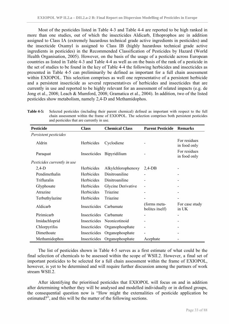
EXIOPOL WP II.2.a – DII.2.a-2 B: Final Report on Dispersion Modelling of Pesticides in Europe
Page 33 of 88
Most of the pesticides listed in Table 4-3 and Table 4-4 are reported to be high ranked in more than one studies, out of which the insecticides Aldicarb, Ethoprophos are in addition assigned to Class IA (extremely hazardous technical grade active ingredients in pesticides) and the insecticide Oxamyl is assigned to Class IB (highly hazardous technical grade active ingredients in pesticides) in the Recommended Classification of Pesticides by Hazard (World Health Organisation, 2005). However, on the basis of the usage of a pesticide across European countries as listed in Table 4-3 and Table 4-4 as well as on the basis of the rank of a pesticide in the set of studies to be found in the key of Table 4-4 the following herbicides and insecticides as presented in Table 4-5 can preliminarily be defined as important for a full chain assessment within EXIOPOL. This selection comprises as well one representative of a persistent herbicide and a persistent insecticide as several representatives of herbicides and insecticides that are currently in use and reported to be highly relevant for an assessment of related impacts (e.g. de Jong et al., 2008; Leach & Mumford, 2008; Gramatica et al., 2004). In addition, two of the listed pesticides show metabolism, namely 2,4-D and Methamidophos.
Table 4-5: Selected pesticides (including their parent chemical) defined as important with respect to the full
chain assessment within the frame of EXIOPOL. The selection comprises both persistent pesticides and pesticides that are currently in use.
Pesticide Class Chemical Class Parent Pesticide Remarks Persistent pesticides
Aldrin Herbicides Cyclodiene - For residues in food only
Paraquat Insecticides Bipyridilium - For residues in food only
Pesticides currently in use 2,4-D Herbicides Alkylchlorophenoxy 2,4-DB - Pendimethalin Herbicides Dinitroaniline - - Trifluralin Herbicides Dinitroaniline - - Glyphosate Herbicides Glycine Derivative - - Atrazine Herbicides Triazine - - Terbuthylazine Herbicides Triazine - -
Aldicarb Insecticides Carbamate (forms meta- bolites itself)
For case study in UK
Pirimicarb Insecticides Carbamate - - Imidachloprid Insecticides Neonicotinoid - - Chlorpyrifos Insecticides Organophosphate - - Dimethoate Insecticides Organophosphate - - Methamidophos Insecticides Organophosphate Acephate -
The list of pesticides shown in Table 4-5 serves as a first estimate of what could be the
final selection of chemicals to be assessed within the scope of WSII.2. However, a final set of important pesticides to be selected for a full chain assessment within the frame of EXIOPOL, however, is yet to be determined and will require further discussion among the partners of work stream WSII.2.
After identifying the prioritised pesticides that EXIOPOL will focus on and in addition
after determining whether they will be analysed and modelled individually or in defined groups, the consequential question now is “How might the externalities of pesticide application be estimated?”, and this will be the matter of the following sections.
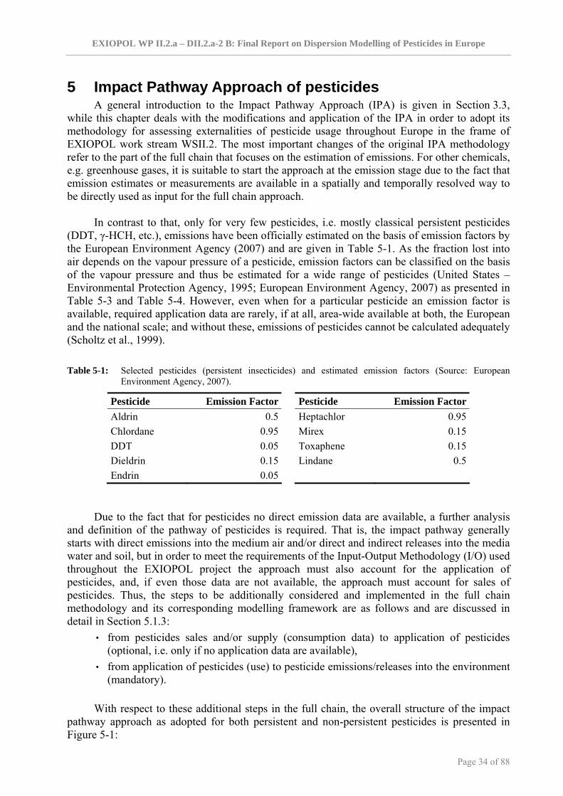
EXIOPOL WP II.2.a – DII.2.a-2 B: Final Report on Dispersion Modelling of Pesticides in Europe
Page 34 of 88
5 Impact Pathway Approach of pesticides A general introduction to the Impact Pathway Approach (IPA) is given in Section 3.3,
while this chapter deals with the modifications and application of the IPA in order to adopt its methodology for assessing externalities of pesticide usage throughout Europe in the frame of EXIOPOL work stream WSII.2. The most important changes of the original IPA methodology refer to the part of the full chain that focuses on the estimation of emissions. For other chemicals, e.g. greenhouse gases, it is suitable to start the approach at the emission stage due to the fact that emission estimates or measurements are available in a spatially and temporally resolved way to be directly used as input for the full chain approach.
In contrast to that, only for very few pesticides, i.e. mostly classical persistent pesticides
(DDT, γ-HCH, etc.), emissions have been officially estimated on the basis of emission factors by the European Environment Agency (2007) and are given in Table 5-1. As the fraction lost into air depends on the vapour pressure of a pesticide, emission factors can be classified on the basis of the vapour pressure and thus be estimated for a wide range of pesticides (United States – Environmental Protection Agency, 1995; European Environment Agency, 2007) as presented in Table 5-3 and Table 5-4. However, even when for a particular pesticide an emission factor is available, required application data are rarely, if at all, area-wide available at both, the European and the national scale; and without these, emissions of pesticides cannot be calculated adequately (Scholtz et al., 1999). Table 5-1: Selected pesticides (persistent insecticides) and estimated emission factors (Source: European
Environment Agency, 2007).
Pesticide Emission Factor Pesticide Emission FactorAldrin 0.5 Heptachlor 0.95Chlordane 0.95 Mirex 0.15DDT 0.05 Toxaphene 0.15Dieldrin 0.15 Lindane 0.5Endrin 0.05
Due to the fact that for pesticides no direct emission data are available, a further analysis and definition of the pathway of pesticides is required. That is, the impact pathway generally starts with direct emissions into the medium air and/or direct and indirect releases into the media water and soil, but in order to meet the requirements of the Input-Output Methodology (I/O) used throughout the EXIOPOL project the approach must also account for the application of pesticides, and, if even those data are not available, the approach must account for sales of pesticides. Thus, the steps to be additionally considered and implemented in the full chain methodology and its corresponding modelling framework are as follows and are discussed in detail in Section 5.1.3:
• from pesticides sales and/or supply (consumption data) to application of pesticides (optional, i.e. only if no application data are available),
• from application of pesticides (use) to pesticide emissions/releases into the environment (mandatory).
With respect to these additional steps in the full chain, the overall structure of the impact
pathway approach as adopted for both persistent and non-persistent pesticides is presented in Figure 5-1:

EXIOPOL WP II.2.a – DII.2.a-2 B: Final Report on Dispersion Modelling of Pesticides in Europe
Page 35 of 88
Figure 5-1: Conceptual structure of a full chain assessment of pesticides following the Impact Pathway Approach
by starting from the use/application of pesticides resulting in emissions/releases into the environment, the fate behaviour and exposure of pesticides as well as the monetary valuation of related welfare losses. Each step of the pathway shows involved media and processes or pathways, respectively. *formation of non-extractable residues. **denotes that for food ingestion not only field crops but also animals, e.g. cattle, are taken into account.
Whereas the process of long-range transport, which is discussed in more detail in Section 5.2.2, is not included in the overall methodology as it does not play a significant role for almost all of the currently used pesticides, two processes have been identified to be very important especially for non-persistent pesticides, namely photo decomposition (also known as photolysis) and chemical decomposition (in particular hydrolysis).
The first part of the pesticide impact pathway approach as shown in Figure 5-1, namely the
Emission Calculation Module, will be discussed in more detail (cf. Section 5.1), which is due to the fact that in this part we face challenges in estimating emissions into the different receiving compartments based on the available data for pesticides sales and application. In contrast to that, the environmental fate as well as the exposure of pesticides can be based on the fate and/or exposure modules of various existing modelling approaches (e.g. EXAMS13, PEARL14, SimpleBox15, Impact 200216, and many more), where most, if not all, relevant processes and 13 http://www.epa.gov/ceampubl/swater/exams/ 14 http://www.pearl.pesticidemodels.eu/ 15 http://www.rivm.nl/bibliotheek/rapporten/672720001.html 16 http://www.sph.umich.edu/riskcenter/jolliet/impact2002.htm

EXIOPOL WP II.2.a – DII.2.a-2 B: Final Report on Dispersion Modelling of Pesticides in Europe
Page 36 of 88
pathways are described in detail. This is different for the impact assessment, which in this study is part of the Exposure and Impact Assessment Module, as most existing modelling approaches base their impact assessment only on data derived from toxicological studies but not from epidemiological studies. In Section 5.4 it will be discussed whether such epidemiologically derived effect information as input for the present impact assessment is available for the selection of prioritised pesticides (cf. Section 4.3.6) and, if so, how to apply this information as so-called dose-response relationships. Finally, the welfare losses, which can directly be derived from the (human health) impacts, and the related monetary valuation, both part of the Valuation Module within the present methodology, are discussed in Section 5.5.
5.1 Estimating emission inventory data The section of the pathway ‘from usage to state of the environment’, within the scope of
work stream WSII.2, comprises the following parts: • The part from the introduction of a pesticide to the market, i.e. the sale or supply of the
product including import and export within the same country as well as from and/or to other countries, to the application of the pesticide, i.e. the use of the product according to current agricultural practise;
• The part from the application of a pesticide to the resulting emissions into air and/or direct and/or indirect releases into water and/or soil17;
• The part from the emission as well as the part between the emissions to the state of the environment, which is hereafter referred to as the environmental fate of pesticides.
Out of these parts, only the part from sales to application and from application to emission will be of concern in this section, while the environmental fate of pesticides is discussed in Section 5.2. First, some general aspects of pesticide inventory data are dealt with, followed by an overview of existing inventory data at the European and in some cases at the national scale, before discussing how to arrive at emissions of pesticides when only sales or application data are available.
5.1.1 General aspects of pesticide inventory data For many substance categories, such as greenhouse gases or several hazardous compounds,
anthropogenic emissions, i.e. direct or indirect releases of a substance into the atmosphere by human activities, e.g. industrial processes and transport, are commonly estimated on the basis of emission factors according to Equation 5-1:
( , , ) ( , , ) ( , , )air airE p z s m p z s emi p z s= ⋅∑ Equation 5-1
where Eair : emission of substance p into the atmospheric compartment of zone z due to
direct releases of source category s [ -1releasedt yr⋅ ]
m : mass of substance p applied in zone z by source category s [ -1appliedt yr⋅ ]
emiair : emission factor of substance p into the atmospheric compartment of zone z from source category s [ -1 -1
released appliedt yr per t yr⋅ ⋅ ].
This common methodological approach combines information about the quantity of a sector- or source category-specific human activity taking place with coefficients that quantify the emissions per a particular unit of this human activity. Those coefficients, just representing simple 17 The different application procedures may result in different lost emission fractions into the environmental media air, water (groundwater and surface water) and soil.

EXIOPOL WP II.2.a – DII.2.a-2 B: Final Report on Dispersion Modelling of Pesticides in Europe
Page 37 of 88
mass balances independently of dealing with (stationary) point, mobile or area sources, are referred to as emission factors and are available, e.g. for greenhouse gases (Intergovernmental Panel on Climate Change, 2006), ‘classical’ air pollutants (United States – Environmental Protection Agency, 1995; 2006), heavy metals (European Environment Agency, 2007) and other contaminants. In many cases, these emission factors are averages of all available activity data of acceptable quality, and are generally assumed to be representative for all facilities in the concerned source category as long as only atmosphere is taken into consideration as receiving environmental compartment.
For the calculation of emissions into atmosphere the European Commission has developed
a strategy in the Atmospheric Emission Inventory Guidebook (European Environment Agency, 2007) how to proceed on the basis of different available or not available data. The whole procedure is shown in Figure 5-2. For the part which is indicated with No. 4 in this procedure (Multiply with emission factor), the United States – Environmental Protection Agency (1995) and the European Environment Agency (2007) have developed emission factors for pesticides on the basis of vapour pressures (cf. Table 5-3 and Table 5-4). How the methodology is applied according to the available data sets regarding sales and application of pesticides at the European as well as at the national level is subject of Section 5.1.3.
Figure 5-2: Flow scheme for the calculation/estimation of pesticides emissions to air by selecting an approach on the basis of data availability. The numbers denote the chronological order of assessing availability of data and calculating emissions from these data, respectively (adapted from European Environment Agency, 2007).
Pesticides emissions, along with emissions of many other contaminants, not only lead to
human health effects via the inhalation pathway, which is almost exclusively related to a chemical’s concentration in the atmospheric compartment, but also imply exposure via oral ingestion18 and/or dermal adsorption (Hamilton & Crossley, 2004; Vida & Moretto, 2007; Juraske, 2007; Simcox et al., 1995). Hence, when conducting a full chain approach as shown in Figure 5-1 by accounting for effects via at least inhalation and ingestion, it would be necessary to also consider further compartments, i.e. different agricultural soils as well as surface and groundwater. This is also because, on average, only a small fraction of the total use of pesticides emits to the atmospheric compartment, ranging from between 1.6% for Bentazone, 3.7% for MCPA and 16% for Pendimethalin in a study in Denmark (Birkved & Hauschild, 2006) to around 25% as average estimate in the Netherlands (Huijsmans, 1995). Additionally, the direct deposition onto plant surfaces, particularly field crops, is to be taken into account as it is a highly
18 Ingestion hereafter refers to both ingestion of different food items and ingestion of drinking water.

EXIOPOL WP II.2.a – DII.2.a-2 B: Final Report on Dispersion Modelling of Pesticides in Europe
Page 38 of 88
relevant way for a pesticide to enter the food chain up to humans (Juraske, 2007; Hamilton & Crossley, 2004).
For a full chain assessment of contaminants, such as pesticides, however, the atmospheric
emissions calculated by means of emission factors as well as direct releases into other environmental media and deposition onto plants serve as initial input to models that, e.g. follow a substance’s pathway through the environmental until its exposure to the receptors of interest. Although on the one hand, for various pesticides emission factors have been derived, but on the other hand, required application data are rarely, if at all, area-wide available at both, the European and the national scale; and without these, emissions of pesticides cannot be calculated (Scholtz et al., 1999), a wide range of modelling tools is available, focussing on the estimation of emissions of plant protection products by means of emission fraction that are lost into different environmental media after application (e.g. Birkved & Hauschild, 2006; Li et al., 2003; Scholtz et al., 1997).
These existing models are mostly based on surface meteorology data to derive emissions
through surface-exchange processes and partly also include a wide range of complexities of volatile compounds, such as dependency on specific physico-chemical properties, meteorology, agricultural practises, etc. In some cases, particularly where a modelling approach not only focuses on the calculation of pesticide emissions but also comprises environmental fate, an exchange model was coupled to one or more transport and/or deposition model(s) in order to comprehensively assess a pesticide’s cycle of emission, deposition and re-emission. Nevertheless, none of these models is a fully integrated, spatially explicit multimedia model, covering all relevant intracompartmental and intercompartmental fate processes on the basis of releases into all considerable media, as well as allowing for an effect assessment calculation via at least inhalation and ingestion exposure, and working at the regional scale.
While a handful of rather generic and local modelling approaches exist which as one part
of the chain estimate pesticide emissions from field application to all environmental media by means of emission fractions (e.g. Birkved & Hauschild, 2006; Margni et al., 2002; Jolliet, 1998), no modelling framework exists that covers the whole chain from application via exposure to external costs for the whole of Europe in a site-specific way. Among some attempts to describe and quantify the external costs of pesticides in a rather general and aggregated way (see Section 5.5 for further details), only one study, namely Leach & Mumford (2008), focussed on the external costs of pesticides in a site-specific way, but only at the local scale. Thus, the present paper sets up a site-specific methodological approach19 at the European scale, taking into account all receiving media for pesticide emissions as well as all relevant exposure pathways and related effect data according to Figure 5-1 in a site-specific way.
However, site-specific pesticide emission calculations on the basis of emission factors are
not suitable for emissions into water and soil, and furthermore, quantitative application data from agriculture are so far only fragmentarily available at the geographical scope to be considered within the scope of EXIOPOL (European Environment Agency, 2007). For instance, according to the Pesticides Safety Directorate, current application data for some sub-national regions of the UK are available for 1990 onwards from the programme of pesticide usage surveys commissioned by the independent Advisory Committee on Pesticides and collected by the Pesticide Usage Surveys Group20 (see Section 5.1.2). In addition, when such data are available, it is still unclear in which spatial resolution and to what sufficiency and thoroughness these 19 It must be noticed at this point that realising a practically applicable modelling tool is beyond the scope of the
project having regard to the overall available person months for pesticide modelling. 20 http://pusstats.csl.gov.uk/

EXIOPOL WP II.2.a – DII.2.a-2 B: Final Report on Dispersion Modelling of Pesticides in Europe
Page 39 of 88
national or sub-national data are provided as mostly data are public only as aggregated values. Hence, with the given time frame of work stream WSII.2 in mind it is not assumed to be able to use those application data as a consistent set for the whole of Europe. More information about currently available application data for different European countries is to be found in the Annex of this document.
If no consistent application data of plant protection products are available for the
geographical scope of interest, it is recommended and common to base the estimation of emission rates on agricultural census and pesticide production or sales data (European Environment Agency, 2007; Benjey, 1993; Economopoulos, 1993) as to be found, for instance, at the Statistical Office of the European Communities, Eurostat (cf. Annex). A review of existing data of sales, application and emissions of pesticides at the European as well as at the national scale, i.e. of countries throughout Europe, has been performed in order to give a first overview of a basis for a consistent pesticide inventory data set that may serve as input for the full chain assessment. The outcome of this review is given in the following section as well as in the detached document ‘MII.2.a-2-National_Pesticide_Inventories.pdf’.
5.1.2 European-wide pesticide inventory data After reviewing several publicly available online data-sets as well as scientific articles and
books for either atmospheric emission factors, application, production or sales/consumption data of pesticides at the European scale, the inventories listed in Table 5-2 could be identified, most of them with different spatial resolutions and/or covering different geographical scopes and years. In addition, in most data-sets only a couple of important pesticides will be found, again underlining the fact that a proper identification of the most relevant agents out of this chemical class is required according to international and national guidelines, which is the matter of Chapter 4.3.1. The data-sets presented in Table 5-2 are described in detail in the following.
Table 5-2: Overview of available inventory data related to emission estimates, reported emissions, emission
factors, applications and/or sales/consumptions of plant protection products at the European or global scale or for selected countries. The IDs are given in order to allocate the entries in this table to the subsequent, more detailed descriptions of the data-sets to be found in ‘Annex A – Pesticides application and/or emission inventory data’.
ID Data Category Data Source Covered Agents Resolution Year(s)
E-1 Emission Estimates
Environment Canada
α-HCH, β-HCH, Toxaphene, (DDT?) 1° x 1° global grid 1980, 1990, 2000
E-2 Emission Estimates MSC-East HCB, γ-HCH
National data, sector-specific or
50km x 50km grid 1990-2004
E-3 Reported Emissions EPER HCB, HCH
National data, sector-specific
(selected countries) 2001, 2004
E-4 Reported Emissions PRTR
Aldrin, Atrazine, Chlordane,
DDT, Endrin, Lindane, Mirex, etc.
National data, sector-specific
Annually, from 2007 onwards (available not before 9/2009)

EXIOPOL WP II.2.a – DII.2.a-2 B: Final Report on Dispersion Modelling of Pesticides in Europe
Page 40 of 88
Table 5-2 (continued)
ID Data Category Data Source Covered Agents Resolution Year(s)
S-1 Sales/ Consumption Eurostat Sum over classes
(e.g. herbicides)
Aggregated national data
(Europe) 1995-2006
S-2 Sales/ Consumption FAOstat
Sum over different classes (herbicides,
organo-phosphates, ...)
Aggregated national data
(World) 1990-2001
S-3 Consumption OECD Sum over classes (e.g. herbicides)
Aggregated national data
(Selected countries) 1980-2006
S-4 Sales BVL 258 active
ingredients in 1055 pesticides
Germany 2006
S-5 Sales MST More than 800 active ingredients Denmark 2005-2007
A-1 Application CSL 455 pesticides United Kingdom 1990-2007
In addition to the emission, sales and/or consumption data obtained for the whole of
Europe also country-specific data have been reviewed, available for different spatial resolutions, such as federal state level, and sometimes only covering a sub-unit of a country, e.g. a specific region or one or more federal states, etc. While at the European level no direct application data are until now available, at least one country, namely the United Kingdom, provides application statistics of active substances for most of its sub-regions (cf. entry A-1 in Table 5-2). Application statistics, however, are the most valuable data serving as input for a full chain approach of pesticides as they are the concrete interface between human activity and the strength of a chemical to the different environmental media. However, a full review of all European country emission and/or application and/or sales data sets is provided in a separate report (cf. detached document ‘MII.2.a-2-National_Pesticide_Inventories.pdf’).
In ‘Annex A – Pesticides application and/or emission inventory data’, all data-sets listed in
Table 5-2 are described in detail by giving some general information related to data integrity, potential limitations, covered active ingredients, trade name chemicals or substance classes, etc., under ‘description’. Furthermore, one or more web links will be provided, at least directly linking to the online data-set, and in some cases also referring to additional explanatory information of these data-sets or further links to involved data, all to be found under ‘URL’. Finally, wherever appropriately applicable, an example is shown under ‘Example’, basically an overview of selected active substances/ingredients or pesticide classes, (selected) countries within Europe or regions within a specific country and specific years, at times helpful for a first general comparison between the data-sets; or just a map, showing the general distribution or development over a given time period for the chemicals of concern.
As the detailed data-sets listed in ‘Annex A – Pesticides application and/or emission
inventory data’ as well as the data-set entries in Table 5-2 belong to different types of pesticide data, e.g. emission estimates or consumption data, all data-sets have been allocated to different data categories by applying a category-specific identification code (ID), i.e.:
• E: Emission estimates (generally obtained by means of a modelling approach), reported emissions due to regulatory obligations or voluntary conventions, or estimated emission

EXIOPOL WP II.2.a – DII.2.a-2 B: Final Report on Dispersion Modelling of Pesticides in Europe
Page 41 of 88
factors for emissions into atmosphere, all rather referring to active substances/ ingredients than to trade products;
• S: Sales or consumption statistics of the agricultural sector, either referring to active substances/ingredients or trade products;
• A: Application data, in principle referring to active substances/ingredients rather than to trade products (note, that although for this category so far no European-wide data-sets exist, this category already is taken into account for future perspectives, e.g. when new international regulations will come into force that claim reporting duties of national application data);
• P: Production statistics, basically comprising production within the selected countries as well as the international trade (import/export) of products, and in principle referring to trade products rather than to active substances/ingredients.
Note, that although for all categories some kind of data are in general available (except application data at the European scale, at least until now, as according to the so far in force being European regulations no duty to report national application data exists within the European Union or beyond, e.g. member states of the European Free Trade Association, EFTA21), they must not necessarily be listed here. Furthermore, some of the data-sets do not fully cover all member states of the European Union, but only a selection, and are, independently from their accuracy, not to be recommended as base for a European pesticide assessment. Some of the listed statistics cover more than the whole of Europe, usually subdivided into equal grid cells at the hemispheric or even global scale. When using these data-sets, however, an intersection is to be performed for achieving data at administrative units, e.g. individual countries, by following the methodology described in Section 3.4 for disaggregating spatial pesticide data.
5.1.3 Linking pesticide sales/application data to emission data Following the methodology presented in Figure 5-2, it is possible to arrive at emission
levels in the environment by starting at whatever data are available, i.e. application, consumption or sales of pesticides. First, when dealing with the term emissions, within the scope of this document, the total fractions of a pesticide applied to a field, which reach the surrounding environment, are meant. With respect to this definition, emissions can occur vertically, i.e. by evaporation or leaching with infiltrating water, or horizontally, i.e. by advection with wind, surface runoff or advection with drainage water (Birkved & Hauschild, 2006). The total emission fraction, femi,total [kgemitted/kgapplied], of a particular pesticide p in a specific zone z can be, hence, quantified as the sum of the fraction emitted to air, femi,air, the fraction emitted to surface water, femi,sw, and the fraction emitted to groundwater, femi,gw, according to Equation 5-2:
, , , ,( , )( , ) ( , ) ( , ) ( , )( , , )
emiemi total emi air emi sw emi gw
applied
m p zf p z f p z f p z f p zm p a z
= = + + Equation 5-2
where memi : mass of pesticide p emitted into the whole environment of zone z [kgemitted] mapplied : mass of pesticide p applied to the field a in zone z [kgapplied].
The processes that are involved in the transport of a pesticide from the application site to the environmental media air, surface water, and groundwater are as follows (note that some of the processes, e.g. evaporation and plant uptake, are competing processes): • Wind drift (depends on the type of application technique, e.g. the height of spray
21 Process of replacing Directive 91/414/EEC http://ec.europa.eu/prelex/detail_dossier_real.cfm?DosId=194494; http://www.europarl.europa.eu/oeil/FindByProcnum.do?procnum=COD/2006/0136).

EXIOPOL WP II.2.a – DII.2.a-2 B: Final Report on Dispersion Modelling of Pesticides in Europe
Page 42 of 88
equipment above ground, and the wind speed); • Deposition onto leaves and/or onto the soil surface (based on crop-specific interception
fractions as, e.g. given in Linders et al., 2000); • Volatilisation from leaves (also known as evaporation; vapour emissions of pesticides
following foliar deposition according to substance specific air-water partition coefficients); • Adsorption (occurs when a pesticide solute accumulates on the surface of an adsorbent, i.e.
plant, soil, or water, thereby forming an adsorbate, which is a homogenous film of molecules).
For the fraction of the pesticide that is lost into air, there exist various approaches on the
basis of emission factors (for a detailed discussion of emission factors please see Section 5.1.1) that generally comprise all processes that contribute to the fraction lost into air. The following Table 5-3 and Table 5-4 present an overview of emission factors as they are used in U.S. and in Europe. According to European Environment Agency (2007), emission factors are derived from the vapour pressure of the pesticides, which is until now the most convenient way to begin the estimation of pesticide emissions, while other estimates may, in addition or instead, take into account Henry coefficient or other parameters, but there are not enough data available to make a more reliable estimate of the emission factors.
Table 5-3: Uncontrolled emission factors for pesticide active ingredients a (Source: United States –
Environmental Protection Agency, 1995).
Emission Factor c Vapour Pressure Range
[mm Hg at 20 to 25°C]b [kg/ton] [dimensionless] Surface application (SCC 24-61-800-001) 1 x 10⁻⁴ to 1 x 10⁻⁶ 350 0.35 >1 x 10⁻⁴ 580 0.58 Soil incorporation (SCC 24-61-800-002) <1 x 10⁻⁶ 2.7 0.0027 1 x 10⁻⁴ to 1 x 10⁻⁶ 21 0.021 >1 x 10⁻⁴ 52 0.052
a Factors are functions of application method and vapour pressure. SCC = Source Classification Code. b For vapour pressures of specific active ingredients see FOOTPRINT Project (Creating tools for pesticide risk
assessment and management in Europe): The FOOTPRINT Pesticide Properties Database (http://www.eu-footprint.org/ppdb.html). Note: for vapour pressure given in [mPa] the conversion factor to [mm Hg] is as follows: 1 mPa ≡ 7.5006 x 10⁻⁶ mm Hg.
c Expressed as equivalent weight of active ingredients volatilized/unit weight of active ingredients applied. (Source: Midwest Research Institute, 1994; Jury et al., 1983).
Table 5-4: Emission factors on the basis of vapour pressure classifications (Source: European Environment Agency, 2007).
Vapour Pressure Vapour pressure class [mPa] [mm Hg]
Emission Factor [dimensionless]
very high >10 >7.5 x 10⁻⁵ 0.95 high 1 to 10 7.5 x 10⁻⁵ to 7.5 x 10⁻⁶ 0.5
average 0.1 to 1 7.5 x 10⁻⁶ to 7.5 x 10⁻⁷ 0.15 low 0.01 to 0.1 7.5 x 10⁻⁷ to 7.5 x 10⁻⁸ 0.05
very low <0.01 <7.5 x 10⁻⁸ 0.01 Note: the conversion of the vapour pressures into [mm Hg] has been done for comparative reasons between the two data source, i.e. United States – Environmental Protection Agency (1995) and European Environment Agency (2007).
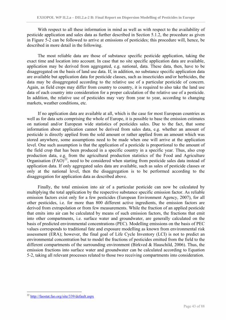
EXIOPOL WP II.2.a – DII.2.a-2 B: Final Report on Dispersion Modelling of Pesticides in Europe
Page 43 of 88
With respect to all these information in mind as well as with respect to the availability of pesticide application and sales data as further described in Section 5.1.2, the procedure as given in Figure 5-2 can be followed to arrive at emissions of pesticides; this procedure will, hence, be described in more detail in the following.
The most reliable data are those of substance specific pesticide application, taking the
exact time and location into account. In case that no site specific application data are available, application may be derived from aggregated, e.g. national, data. These data, then, have to be disaggregated on the basis of land use data. If, in addition, no substance specific application data are available but application data for pesticide classes, such as insecticides and/or herbicides, the data may be disaggregated according to the relative use of a particular pesticide of concern. Again, as field crops may differ from country to country, it is required to also take the land use data of each country into consideration for a proper calculation of the relative use of a pesticide. In addition, the relative use of pesticides may vary from year to year, according to changing markets, weather conditions, etc.
If no application data are available at all, which is the case for most European countries as
well as for data sets comprising the whole of Europe, it is possible to base the emission estimates on national and/or European wide statistics of pesticides sales. Due to the fact, that some information about application cannot be derived from sales data, e.g. whether an amount of pesticide is directly applied from the sold amount or rather applied from an amount which was stored anywhere, some assumptions need to be made when one will arrive at the application level. One such assumption is that the application of a pesticide is proportional to the amount of the field crop that has been produced in a specific country in a specific year. Thus, also crop production data, e.g. from the agricultural production statistics of the Food and Agriculture Organisation (FAO)22, need to be considered when starting from pesticide sales data instead of application data. If only aggregated sales data are available, such as sales of pesticide classes or only at the national level, then the disaggregation is to be performed according to the disaggregation for application data as described above.
Finally, the total emission into air of a particular pesticide can now be calculated by multiplying the total application by the respective substance specific emission factor. As reliable emission factors exist only for a few pesticides (European Environment Agency, 2007), for all other pesticides, i.e. for more than 800 different active ingredients, the emission factors are derived from extrapolation or from few measurements. While the fraction of an applied pesticide that emits into air can be calculated by means of such emission factors, the fractions that emit into other compartments, i.e. surface water and groundwater, are generally calculated on the basis of predicted environmental concentrations (PEC). Modelling emissions on the basis of PEC values corresponds to traditional fate and exposure modelling as known from environmental risk assessment (ERA); however, the final goal of Life Cycle Inventory (LCI) is not to predict an environmental concentration but to model the fractions of pesticides emitted from the field to the different compartments of the surrounding environment (Birkved & Hauschild, 2006). Thus, the emission fractions into surface water and groundwater can be calculated according to Equation 5-2, taking all relevant processes related to those two receiving compartments into consideration.
22 http://faostat.fao.org/site/339/default.aspx

EXIOPOL WP II.2.a – DII.2.a-2 B: Final Report on Dispersion Modelling of Pesticides in Europe
Page 44 of 88
5.2 Multimedia environmental fate of pesticides
5.2.1 Considered environmental fate processes of pesticides As, in general, a wide range of models exist that deal with the environmental fate of
organic pollutants, such as pesticides, the processes that these chemicals undergo in the environment are well described and will not be discussed in detail in the present document. Types of modelling frameworks dealing with the environmental fate of organic pollutants in general and/or with the environmental fate of pesticides in particular can be multimedia box models, such as SimpleBox 3.0, which was developed at the National Institute of Public Health and the Environment (RIVM), or chemical transport models, such as MSCE-POP, which was developed at the Meteorological Synthesizing Centre – East (MSC-E). Furthermore, modelling frameworks may focus on specific fate processes only, such as MACRO, a model focussing on water flow and reactive solute transport of pesticides in field soils, which was developed at the Swedish University of Agricultural Sciences (SLU). All relevant processes to be considered in the Environmental Fate Module of the full chain approach of pesticides according to Figure 5-1 are presented in Table 5-5. Table 5-5: Processes that are considered with respect to the environmental fate of persistent as well as non-
persistent pesticides as to be implemented in the Environmental Fate Module of the full chain assessment of pesticides within EXIOPOL.
Environmental fate processes relevant for pesticides
Process Description Remarks
Sorption (adsorption/ desorption)
Attraction of the molecules of a substance in gaseous or liquid form to the surface of a solid (e.g. non-polar pesticides tend to be pushed out of water and onto soils which contain non-polar carbon material; metal ions tend to adsorb at oxide mineral-water interfaces) and its reverse process. d OC OCK K f= ⋅ Kd: Sorption coefficient or distribution coefficient or soil-water
partition coefficient [L/kg]: ratio of the sorbed concentration of a substance [mg/kg] per concentration of the substance in solution [mg/L].
KOC: Soil organic carbon-water partition coefficient [L/kg]: ratio of the mass of a substance in the organic fraction of the soil [kg] per mass of organic carbon in the soil [kg] per concentration of the substance in solution [mg/L]; depends on the physico-chemical properties of the substance, not on the percent of organic matter in the soil. Assumption: predominant sorbent in soil is the soil organic matter (SOM).
fOC: Mass fraction of soil organic carbon content [kg/kg].
Sorption can be calculated by means of the Freundlich Equation.
Also relevant as process in the Emission Calculation Module.
Formation of non-extractable residues
Formation of a portion of an introduced substance that is non-extractable by a simulated soil solution or organic solvents after a specific period of sorption to soil organic matter. This portion is referred to as non-extractable residue (NER) and can refer to parent molecules and/or metabolites.
-
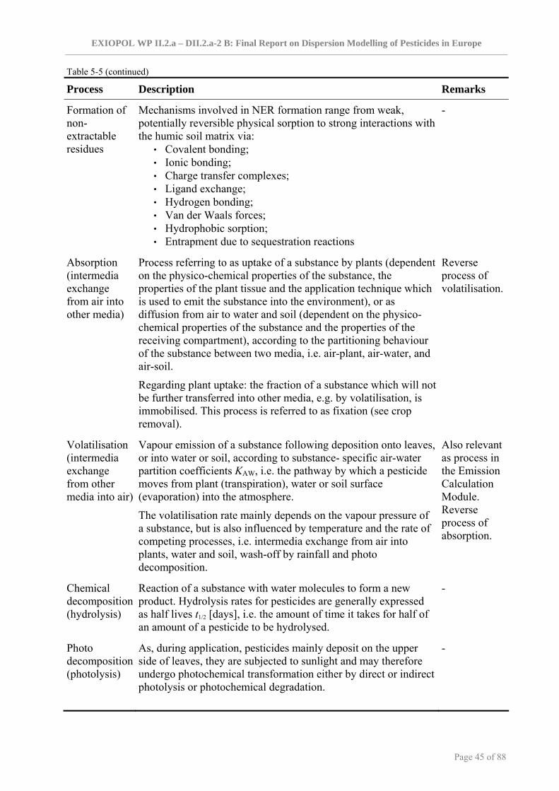
EXIOPOL WP II.2.a – DII.2.a-2 B: Final Report on Dispersion Modelling of Pesticides in Europe
Page 45 of 88
Table 5-5 (continued)
Process Description Remarks
Formation of non-extractable residues
Mechanisms involved in NER formation range from weak, potentially reversible physical sorption to strong interactions with the humic soil matrix via: • Covalent bonding; • Ionic bonding; • Charge transfer complexes; • Ligand exchange; • Hydrogen bonding; • Van der Waals forces; • Hydrophobic sorption; • Entrapment due to sequestration reactions
-
Absorption (intermedia exchange from air into other media)
Process referring to as uptake of a substance by plants (dependent on the physico-chemical properties of the substance, the properties of the plant tissue and the application technique which is used to emit the substance into the environment), or as diffusion from air to water and soil (dependent on the physico-chemical properties of the substance and the properties of the receiving compartment), according to the partitioning behaviour of the substance between two media, i.e. air-plant, air-water, and air-soil.
Regarding plant uptake: the fraction of a substance which will not be further transferred into other media, e.g. by volatilisation, is immobilised. This process is referred to as fixation (see crop removal).
Reverse process of volatilisation.
Volatilisation (intermedia exchange from other media into air)
Vapour emission of a substance following deposition onto leaves, or into water or soil, according to substance- specific air-water partition coefficients KAW, i.e. the pathway by which a pesticide moves from plant (transpiration), water or soil surface (evaporation) into the atmosphere.
The volatilisation rate mainly depends on the vapour pressure of a substance, but is also influenced by temperature and the rate of competing processes, i.e. intermedia exchange from air into plants, water and soil, wash-off by rainfall and photo decomposition.
Also relevant as process in the Emission Calculation Module. Reverse process of absorption.
Chemical decomposition (hydrolysis)
Reaction of a substance with water molecules to form a new product. Hydrolysis rates for pesticides are generally expressed as half lives t1/2 [days], i.e. the amount of time it takes for half of an amount of a pesticide to be hydrolysed.
-
Photo decomposition (photolysis)
As, during application, pesticides mainly deposit on the upper side of leaves, they are subjected to sunlight and may therefore undergo photochemical transformation either by direct or indirect photolysis or photochemical degradation.
-

EXIOPOL WP II.2.a – DII.2.a-2 B: Final Report on Dispersion Modelling of Pesticides in Europe
Page 46 of 88
Table 5-5 (continued)
Process Description Remarks
Photo decomposition (photolysis, photo dissociation)
Direct photolysis: a substance absorbs light and then undergoes a transformation reaction from an excited state. Indirect photolysis: naturally occurring compounds absorb energy via sunlight which is then transferred to a substance of concern, to form free OH-radicals or promote redox reactions that result in the transformation of the substance.
-
Biological degradation (metabolism)
Occurs via enzymatic catalysis by microorganisms and can follow complex pathways involving a variety of interactions among microorganisms, soil constituents, and substances of concern. Thus, biological degradation rates depend on the physico-chemical properties of the substance but also on microbiological and physico-chemical properties of the soil as well as soil temperature and moisture. Note that, aside from biological degradation, also abiotic degradation may result in metabolites.
Biological as well as abiotic degradation of a substance may lead to detoxication, which refers to the metabolic process of a substance by which the parent chemical yields less toxic derivatives which are more soluble in water.
-
Crop removal Refers to the removal of a pesticide across the boundaries of the Environmental Fate Module of the modelling framework due to uptake by plants (see absorption) followed by harvest.
Regarding fixation: the fraction of a substance which was absorbed via plant uptake and that was not be further transferred into other media, e.g. by volatilisation, has been immobilised only until crop removal.
Ultimate fate process but, however, relevant for the Exposure and Impact Assessment Module.
Water-soil erosion
Removal of soil surface material, i.e. wearing away and transport of the soil by running water, glaciers, wind or waves, while water and wind are the major agents. The erosion potential of a soil strongly depends on the soil texture.
Most prevalent types of soil erosion by water: • Sheet erosion: combination of downslope movement of
splash and surface water. • Rill/inter-rill erosion: surface water movement to or
between small depressions (ephemeral concentrated flow paths), where the water gains depth and velocity.
• Gully erosion: formation of channels (U-shaped, V-shaped) in soils due to increase in water depth, velocity and volume.
Note that water-soil erosion is relevant only for strongly sorbing substances, i.e. around KOC > 1000 L/kg (cf. sorption).
-

EXIOPOL WP II.2.a – DII.2.a-2 B: Final Report on Dispersion Modelling of Pesticides in Europe
Page 47 of 88
Table 5-5 (continued)
Process Description Remarks
Surface run-off
Refers to the overland flow of a substance, which is the flow of water including the dissolved fraction of a substance over the ground before it enters a definite channel, occurring when the infiltration capacity of a soil, i.e. the saturated hydraulic conductivity of a soil, is exceeded by the rainfall intensity (infiltration excess run-off) or when rain is falling on soil that is already saturated (saturation excess run-off).
Note that surface run-off with respect to assessing the environmental fate behaviour of pesticides does not equal run-off with respect to hydrology in general. The latter refers to the quantity of water that is discharged in surface streams.
-
Lateral subsurface flow
Precipitation infiltrates and is transported downslope through the soil profile. This transport process can be quite rapid in shallow, well structured soils overlaying clay or bedrock and takes place almost exclusively along paths of preferential flow (cf. leaching). Lateral subsurface flow strongly depends on the antecedent soil-moisture.
-
Drainage (drain flow)
Refers to the loss of pesticides from fields via removal of excess water from the soil through field drains. The total drainage cannot exceed the saturated hydraulic conductivity of a soil.
-
Leaching
Downward vertical movement of a substance with percolating water in the soil profile and the unsaturated zone towards the groundwater table. Leaching of pesticides usually occurs in dissolved form. It has been shown, however, that colloid-facilitated transport can play an important role for leaching of strongly sorbing pesticides.
Leaching can occur via matrix flow (in the soil matrix, following the Richard’s equation) or via preferential flow of water (e.g. in macropores, cracks, rodent tunnels, root channels).
-
Combined environmental fate processes relevant for pesticides
Process Description Remarks
Dissipation Volatilisation, photo decomposition, chemical decomposition, biological degradation, intermedia exchange (including plant uptake)
Occurs directly after application.
Degradation Chemical decomposition, photo decomposition, biological degradation
-
Long-range transport
Volatilisation (in particular re-emission), deposition (dry), deposition (wet), wind drift, water-soil erosion
Only regards persistent pesticides.

EXIOPOL WP II.2.a – DII.2.a-2 B: Final Report on Dispersion Modelling of Pesticides in Europe
Page 48 of 88
Some of the processes, such as volatilisation and absorption, are involved in the process termed long-range transport, which is particularly important for persistent pesticides and will, hence, be further discussed in Section 5.2.2.
All of the processes listed in Table 5-5 depend on various parameters, e.g. the physico-
chemical properties of the pesticides, the environmental conditions, etc. Most of the important substance specific parameters, such as octanol-water partition coefficient, vapour pressure or soil degradation DT50, can be derived from databases, e.g. the FOOTPRINT Pesticide Properties Database (http://www.eu-footprint.org/ppdb.html) for as many as 750 active ingredients as well as 350 metabolites, or from handbooks of pesticide properties, e.g. Mackay et al. (1997) for 170 active ingredients. In addition, many more existing data resources of substance specific properties have been reviewed and are presented in Boethling et al. (2004). With the knowledge about the processes and the related parameters, a modelling framework of the environmental fate of both persistent and non-persistent pesticides can be set up accordingly.
5.2.2 Discussion of persistence and long-range transport Due to the fact that on the one hand many of the classical pesticides23, which are also
known to be listed in the annex of the POPs Convention24, are persistent, while on the other hand most currently used pesticides have been developed with the intention not to resist in the environment for a long time, the term persistence needs to be discussed in more detail.
“The term persistence was introduced into the pesticide scientific literature to describe the
continuing existence of certain insecticides in the environment and is now applied to any organic chemical that has biological activity.” (Greenhalgh, 1980, p. 2565). In contrast to persistence, the terms stable and inert, which are commonly encountered in chemistry and physics, are not appropriate since they do not properly characterise the nature of persistent chemicals, that is, some degradation almost always occurs and, in fact, some persistence is desirable (ibid.). While ideally a pesticide is used with the intention to effectively control a target organism for a critical period of time, which generally is during its growth period, and then degrade to products harmless to humans and the environment, the reality is something different. In practice, the usage of some pesticides may lead to the continued existence of the parent compound and, in some cases, biologically active metabolites over prolonged periods. On the basis of these considerations, it is essential to estimate for how long any pesticide of concern persists after its regular application, assuming that this is in line with good agricultural practice25. Furthermore, it is of importance to know about the possible implications of the persistence of such a pesticide, i.e. its potential for bioaccumulation and/or selective toxicity.
With increased concern over the long term effects of pesticides in various environments,
the idea has developed that persistence is a measurable property of a chemical, representing its resistance to changes of its chemical structure. This is an oversimplification, since the period over which a chemical exerts an effect depends on its properties, the characteristics of the specific environment and the concerned organisms. Hence, persistence does not denote an absolute characteristic of a chemical, but is a variable which is a function of many interactions which leads us to the following question: “How can persistence be generally defined?”
23 The term classical pesticide, within this document, is used to describe the pesticides that have been developed and widely used during the last six decades and generally comprise the well-known insecticides DDT, Lindane, Aldrin, Chlordane, Heptachlor, and others. 24 Stockholm Convention on Persistent Organic Pollutants (http://chm.pops.int/) 25 Good agricultural practices are hereafter referred to as practices that address environmental, economic and social sustainability for on-farm processes, and result in safe and quality food and non-food agricultural products according to the definition of the Food and Agriculture Organization of the United Nations (http://www.fao.org/prods/GAP/).

EXIOPOL WP II.2.a – DII.2.a-2 B: Final Report on Dispersion Modelling of Pesticides in Europe
Page 49 of 88
The term persistence is differently employed by scientists in many disciplines. An
agronomist, for instance, has to consider whether a pesticide will survive long enough to control a problem, and also whether it will leave toxic residues that may adversely affect the future use of soils or crops. In contrast to that, the analytical chemist determines the measurable presence of a chemical in a specific medium at a specific period of time, regardless of its bioavailability or effects to humans or the environment. As a third example, the toxicologist examines the effects of different food items containing residues of the parent pesticide or relevant metabolic products for human health safety. Last but not least, the ecologist is interested in the even wider environmental problems caused by pesticide dispersal such as adverse effects in non-target organisms. In addition, the term persistence appears in numerous scientific and popular publications, where the actual meaning, with respect to the limits prescribing its use, is not described. Because of the varied use of the term, persistence will be defined, within the context of the EXIOPOL work stream WSII.2, according to the requirements of pesticide chemistry. Persistence, hence, can be defined as the “residence time of a chemical species in a specifically defined compartment of the environment” (Greenhalgh, 1980, p. 2566), where a chemical species is a specific chemical, which may be the parent pesticide or a derivative, but not both; the residence time is the period in which the specific chemical species remains in one compartment, regardless of the means by which it is quantified26; and a compartment is one phase of the environment, i.e. soil, water, air, animal or plant tissues. This definition is concerned only with the physico-chemical properties of the chemical species in its immediate compartment of the environment. The dispersal, i.e. translocation and bioaccumulation, of the pesticide from its primary compartment will necessitate a further determination of persistence. Consequently, a pesticide will have a specific persistence in each compartment where it is present. The consequences of persistence, as related to the toxicity and bioavailability of the pesticide, however, are not considered.
In general, persistence and, hence, the potential to undergo the process of long-range
transport, only play a significant role for few pesticides, e.g. most classical persistent pesticides, whereas almost all pesticides that are currently in use have been developed with the intention to rapidly degrade after accomplishing the task for what they have been produced. Thus, long-range transport will only be included for the assessment of such selected pesticides (cf. Section 4.3.6) that are assigned to the category of Persistent Organic Pollutants as declared in Annex D of the Stockholm Convention of Persistent Organic Pollutants.
Long-range transport, however, is an important process with respect to most of the
classical persistent pesticides, and will thus briefly be discussed in the following. Generally, the ability of a chemical to be transported over large distances is the result of complex interactions between its environmental phase distribution and persistence in various phases. Persistence alone is not sufficient for a long-range transport potential (LRTP) in air and water, i.e. a pesticide must also be semi-volatile (Matthies & Scheringer, 2001). In addition, the inter-media mass exchange processes between air, water, soil, and sediment, and the transformation in these media under spatially and temporally variable environmental conditions, also have to be taken into account to determine the transport and fate of persistent pesticides, and atmospheric wind and turbulence as well as ocean currents are the driving forces for their global distribution. Temperature, furthermore, plays an important role in the explanation of high concentrations found in remote regions, such as the Arctic, due to the so-called cold condenser effect. In order to assess all the simultaneous processes, they can be integrated by means of multimedia modelling frameworks, 26 The residence time is measured in units of time, day, year, etc. When (pseudo) first order processes occur, it is simply (1/k) where k is the first order rate constant. If the order is unknown, the time for 50% disappearance (DT50) at specific initial concentrations can be used.
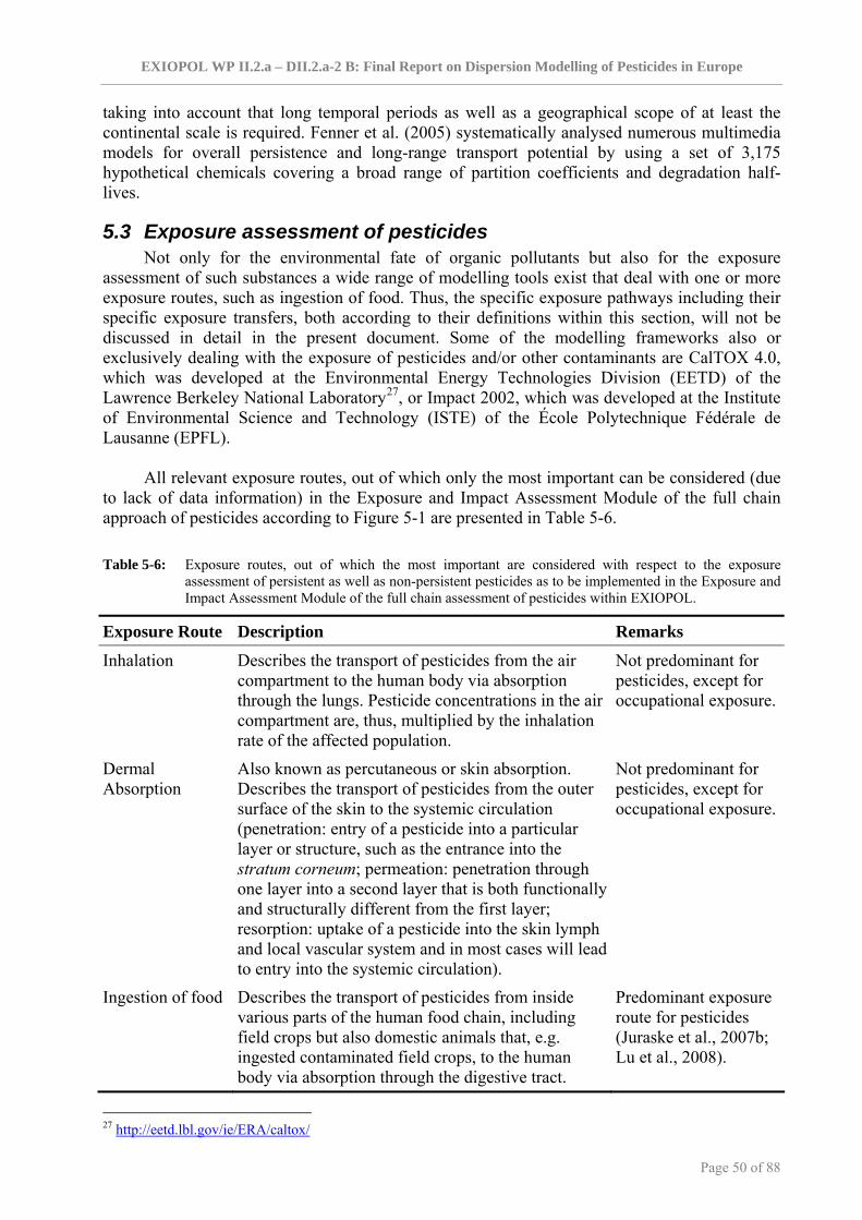
EXIOPOL WP II.2.a – DII.2.a-2 B: Final Report on Dispersion Modelling of Pesticides in Europe
Page 50 of 88
taking into account that long temporal periods as well as a geographical scope of at least the continental scale is required. Fenner et al. (2005) systematically analysed numerous multimedia models for overall persistence and long-range transport potential by using a set of 3,175 hypothetical chemicals covering a broad range of partition coefficients and degradation half-lives.
5.3 Exposure assessment of pesticides Not only for the environmental fate of organic pollutants but also for the exposure
assessment of such substances a wide range of modelling tools exist that deal with one or more exposure routes, such as ingestion of food. Thus, the specific exposure pathways including their specific exposure transfers, both according to their definitions within this section, will not be discussed in detail in the present document. Some of the modelling frameworks also or exclusively dealing with the exposure of pesticides and/or other contaminants are CalTOX 4.0, which was developed at the Environmental Energy Technologies Division (EETD) of the Lawrence Berkeley National Laboratory27, or Impact 2002, which was developed at the Institute of Environmental Science and Technology (ISTE) of the École Polytechnique Fédérale de Lausanne (EPFL).
All relevant exposure routes, out of which only the most important can be considered (due to lack of data information) in the Exposure and Impact Assessment Module of the full chain approach of pesticides according to Figure 5-1 are presented in Table 5-6. Table 5-6: Exposure routes, out of which the most important are considered with respect to the exposure
assessment of persistent as well as non-persistent pesticides as to be implemented in the Exposure and Impact Assessment Module of the full chain assessment of pesticides within EXIOPOL.
Exposure Route Description Remarks
Inhalation Describes the transport of pesticides from the air compartment to the human body via absorption through the lungs. Pesticide concentrations in the air compartment are, thus, multiplied by the inhalation rate of the affected population.
Not predominant for pesticides, except for occupational exposure.
Dermal Absorption
Also known as percutaneous or skin absorption. Describes the transport of pesticides from the outer surface of the skin to the systemic circulation (penetration: entry of a pesticide into a particular layer or structure, such as the entrance into the stratum corneum; permeation: penetration through one layer into a second layer that is both functionally and structurally different from the first layer; resorption: uptake of a pesticide into the skin lymph and local vascular system and in most cases will lead to entry into the systemic circulation).
Not predominant for pesticides, except for occupational exposure.
Ingestion of food Describes the transport of pesticides from inside various parts of the human food chain, including field crops but also domestic animals that, e.g. ingested contaminated field crops, to the human body via absorption through the digestive tract.
Predominant exposure route for pesticides (Juraske et al., 2007b; Lu et al., 2008).
27 http://eetd.lbl.gov/ie/ERA/caltox/

EXIOPOL WP II.2.a – DII.2.a-2 B: Final Report on Dispersion Modelling of Pesticides in Europe
Page 51 of 88
Table 5-6 (continued)
Exposure Route Description Remarks Ingestion of drinking water
Describes the transport of the dissolved fractions of pesticides from the water compartment, i.e. surface water and groundwater, to the human body via absorption through the digestive tract.
Not predominant for pesticides.
Ingestion of other than food and drinking water
Describes the transport of pesticides from the soil compartment to the human body via absorption through the digestive tract, particularly refers to unintended ingestion of soil particles by children as deliberate soil ingestion, also termed pica, is considered relatively uncommon.
Not predominant for pesticides.
Note that all of the listed exposure routes are to considered as important, even though they are listed as ‘not predominant’.
As ingestion of food items is reported to be the predominant exposure route of pesticides (Juraske et al., 2007a, 2007b; Lu et al., 2008), it will be described in more detail in the following. The exposure assessment of food products may be very complex due to both the variety of food items to which human beings might be exposed and the spatial distribution of the food production. The exposure assessment follows administrative units taking the availability of food and population data into account, where the national and international trade of the different food products that are taken into consideration for the exposure assessment of pesticides is considered as an extension of the (natural) environmental fate of the pesticides. The concept of the Intake Fraction (Bennett et al., 2002) is used as a measure for the overall exposure. The Intake Fraction is only given for those portions of a contaminant that may cause an adverse effect and is, therefore, described as ’effective’. It is the fraction of the mass of a pesticide released into the environment that is ultimately taken in by the human population as a result of food and/or drinking water consumption, inhalation and/or dermal exposure. In case of food ingestion, this implies that it aggregates the exposure towards different produces, which may become contaminated due to different causes. Each such cause-exposure chain starting at the result of the environmental fate model is hereafter termed exposure pathway (cf. next clause). The intake fraction due to ingestion exposure is calculated as:
( , , , ) ( )( , , , )
( , , )personal population
total
IR p e r b n biF p e i b
S p k b⋅
= ∑ Equation 5-3
where iF : effective intake fraction of pesticide p via a specific exposure pathway e for a
certain population i in country b [kgintake per kgreleased] IRpersonal : effective personal intake rate of pesticide p via a specific exposure pathway e
related to produce/food item r in country b [kgintake·capita-1·s-1]. Note that this parameter does not need to be taken into account when dealing with inhalation exposure of pesticides.
npopulation : population in country b [capita] S : source strength of a pesticide p into compartment k of all countries btotal
[kgreleased·s-1]. Within the Exposure and Impact Assessment Module as defined in Figure 5-1 for some of
the exposure routes of pesticides, such as ingestion of food, different exposure pathways are
EXIOPOL WP II.2.a – DII.2.a-2 B: Final Report on Dispersion Modelling of Pesticides in Europe
Page 52 of 88
considered. Exposure pathway (or food chain) in this context refers to any combination of (a) an environmental medium concentration as predicted by the Environmental Fate Module (e.g. agricultural soil concentration) based on which (b) different interrelated intermediate food concentrations are derived (e.g. wheat consumed by cow, milk) finally being (c) taken in by humans. This brings about that human exposure for example to milk is composed of the exposure pathways based on the ingestion of soil particles, forage, silage and grains by milk cattle. Each of the linkages or steps of an exposure pathway is termed an exposure transfer, i.e. a transfer from one medium, substrate, or receptor to another. Regarding the ingestion of different food items, the Environmental Fate Module should results in bulk concentrations that are given in weight of a pesticide per volume of a medium [kg/m3]. However, many of the equations in the exposure assessment of terrestrial food chains will be based on concentrations that are given in weight of a substance per (dry or fresh) weight of the medium [kg/kg fresh weight or kg/kg dry weight] according to United States – Environmental Protection Agency (1998). The food chains in the aquatic environment, in contrast, will be based on the dissolved fraction of a pesticide. Consequently, different unit conversions need to be performed in order to arrive at a specific exposure.
5.4 Human health impact assessment of pesticides According to the International Programme on Chemical Safety (IPCS) it is most difficult to
establish exposure-response relationships for human exposure of pesticides, in particular of pesticides currently in use, and incident disease. Humans encounter a broad range of environmental exposures and frequently to a mixture of chemicals at any one time. Much work remains to be done on the study of the human health impacts of exposure to persistent and non-persistent pesticides, particularly in view of the broad range of concomitant exposing experienced by humans (Ritter et al., 2001). The methodology how to derive human health endpoint related information to be integrated into a full chain assessment of selected pesticides will be further explained in the following.
Much of the health information will relate to pesticide compounds used historically, and
not necessarily those in common usage now; though across Europe, there will be some variations in usage, so that what was used historically in one region may still be in current use in another etc. However, there are basically two approaches available for deriving effect information related to pesticides. One approach is via epidemiology, and what it tells us about exposure-response relationships linking specific (chemical classes of) pesticides with defined adverse human health effects. The most important part, besides the exposure-response information themselves, is to focus on how the exposure-response part of the full chain links in with other aspects, such as the amount of a pesticide (class) that is applied in a particular country for which an exposure-response relationship is available. Insofar as there are usable exposure-response relationships available, they have to be seen in the context of:
• What active ingredient or chemical class of pesticides these relate to, • What exposure metrics these relate to, • What health effects (health endpoints) are relevant, to what extent these are the same for
different kinds of pesticides, • What is known about thresholds and/or other nonlinearities in the exposure-response
relationship, • What is known about susceptible populations or sub-population groups, • What if any effects modifiers are important.

EXIOPOL WP II.2.a – DII.2.a-2 B: Final Report on Dispersion Modelling of Pesticides in Europe
Page 53 of 88
A second approach is via understanding of mechanisms, i.e. through detailed Physiologically-based pharmacokinetic modelling (PBPK modelling) of the part of the pathway that starts at exposure (e.g. by ingestion, inhalation or dermal exposure) through dose to the target organ to the risk of an adverse health effect. Within the HEIMTSA project, this approach is being developed by partners at the JRC.
Independently of what approach finally will be applied for arriving at human health effect information that can be linked to finally yield unit values of pesticides due to agricultural practice, the full chain approach is much simpler if the exposure-response relationship is linear, i.e. without threshold. Even if the evidence does not support this view, with respect to the scope of EXIOPOL, we will, as a first step, make the simplifying assumption of linear, no-threshold exposure-response relationships, in order to get an order-of-magnitude on the health effects associated with (a) some baseline usage and (b) the change in exposure associated with a change in policy.
For an initial look, we have sought out reviews of the health effects of pesticides, from human epidemiological studies (Maroni and Fait, 1993; Alvanja et al, 2004; Sanborn et al, 2004; plus confidential material from an ongoing study not yet published). Almost all of the studies reviewed have been from studies of occupational populations, with some additional data from bystander populations exposed to industrial-scale operations such as crop-spraying. The findings are variable, and are often not specific to individual chemicals, or even to general classes of chemical; a summary of the consensus available from these reviews is in Annex
From a policy point of view it also has to be discussed, up to what extent it is generally
possible to reduce human health impacts caused by agricultural activities. This is due to the fact that a significant fraction of the overall estimated health effects may not stem from legal and official agricultural practice which is known as «good agricultural practice», i.e. practice that addresses environmental, economic and social sustainability for on-farm processes, and results in safe and quality food and non-food agricultural products according to the definition of the Food and Agriculture Organization of the United Nations (http://www.fao.org/prods/GAP/). It may rather be the fact that a considerable fraction of the effects is related to the illegal use of pesticides as e.g. reported by the European Crop Protection Association, ECPA28, or to misuse as well as accidents during the application or transport of pesticides. This leads to the question of how can policy deal with these effects? However, as it seem to play a significant role with respect to the overall health effects caused by pesticides, it has to be discussed in a wider policy context to not only e.g. prohibit or ban particular compounds but also to include educational and other aspects for successfully reducing the risk of the population to get affected by inhaling, touching or ingesting pesticides.
5.5 Valuation of pesticide impacts Various attempts have been made not only to describe but also to quantify the negative
impacts of pesticides to the environment and human health. Some of these attempts include research in the USA (Pimentel et al., 1992; Pimentel, 2005; Tegtmeier & Duffy, 2004), in the UK (Pretty et al., 2000) and in the UK, USA and Germany (Pretty et al., 2001; Leach & Mumford, 2008). However, as these studies either considered the combined costs of all pesticides at a country level or the costs of individual pesticides at a local scale, an approach of site-specific externality assessment on the basis of selected pesticides at various scales is still not available. The aim of this work stream WSII.2, thus, is to provide a comprehensive
28 ECPA (2008) 12 Arrested and 5 tonnes of product confiscated as police sweep Andalucia, Spain for Illegal
pesticides (http://www.ecpa.be/website/page.asp?mi=1&cust=3&lang=en&news=18280).

EXIOPOL WP II.2.a – DII.2.a-2 B: Final Report on Dispersion Modelling of Pesticides in Europe
Page 54 of 88
methodological as well as modelling approach to not only to assess the impacts of pesticides in a spatially and temporally resolved way for the geographical scope of Europe, but also to values these impacts to end up at external costs, which on their part can be used as input for the Input-Output Methodology (I/O) used throughout the EXIOPOL project.
The quantification of external costs will be performed in two steps, namely (i) the
weighting of the quantified human health impacts by means severity measures, such as Disability Adjusted Life Years, and (ii) the monetisation by means of monetary values for each severity measure. The procedure how to end up at external cost, hence, is described in more detail in the following.
5.5.1 Weighting of pesticide impacts by means of severity measures From a valuation perspective, it is necessary to distinguish between diverse human health
effects as ’effects’ in general may lead to consequences with different severities like acute death or some short-lived skin irritation. In case of fatal diseases, the concept of Years of Life Lost (YOLL) is recommended in different contexts (Krewitt et al., 2002). The YOLL indicator measures the reduction in life expectancy resulting from an increased level of exposure to pollutants in the environment. In order also to account for effects related to morbidity, Crettaz et al. (2002) and Pennington et al. (2002) make use of the Disability Adjusted Life Years (DALY) concept. It comprises the effects measured by the YOLL indicator and adds the measure Years of Life lived with a Disability (YLD). Although the approach has some disadvantages related to the derivation of the YLD and when applied to non-cancer effects, it is deemed a step towards a more differentiated assessment of cancers for whose valuation only one generic monetary value for any type of cancer is used according to the latest ExternE methodology (Bickel & Friedrich, 2005). In addition, for some human health endpoints the severity measure IQ Points Loss was introduced, in particular for the weighting of neurotoxic diseases, for which no DALY can be derived so far. The severity measures YOLL, YLD and IQ Points Loss can be calculated according to Equation 5-4, while the aggregated measure DALY is calculated according to Equation 5-5:
( )∑=
⋅=totalt
tincidencesseverity ehpsmfbihepnbiehpn
1),,(),,,,(),,,,( Equation 5-4
where nseverity : number of a specific severity measure per human health end-point h due to
intake of pesticide p via a specific exposure pathway e by a certain population i in country b [YOLL; YLD; IQ Points Loss]; note that nseverity only refers to ‘Years of Life Lost’, ‘Years of Life lived with a Disability’ and ‘IQ Points Loss’
t : year for which an annual amount of external costs has been calculated [yr] ttotal : time span for which the total external costs have been calculated [yr] as sum
of all annual external costs within the considered time span [yr] nincidences : number of incidences of human health end-point h due to intake of pesticide p
via a specific exposure pathway e by a certain population i in country b [-] smf : severity-measure factor per incidence of human health end-point h due to
intake of pesticide p via a specific exposure pathway e [YOLL·incidence-1; YLD·incidence-1; IQ Points Loss·incidence-1].
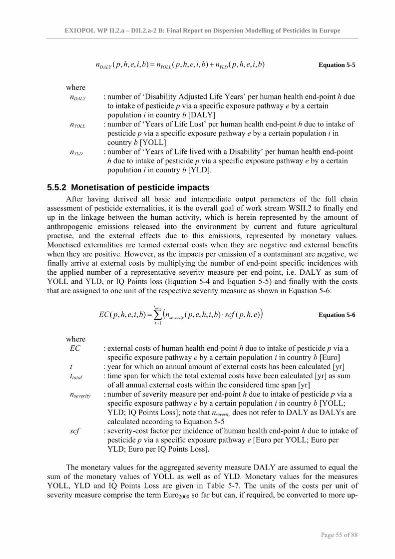
EXIOPOL WP II.2.a – DII.2.a-2 B: Final Report on Dispersion Modelling of Pesticides in Europe
Page 55 of 88
),,,,(),,,,(),,,,( biehpnbiehpnbiehpn YLDYOLLDALY += Equation 5-5
where nDALY : number of ‘Disability Adjusted Life Years’ per human health end-point h due
to intake of pesticide p via a specific exposure pathway e by a certain population i in country b [DALY]
nYOLL : number of ‘Years of Life Lost’ per human health end-point h due to intake of pesticide p via a specific exposure pathway e by a certain population i in country b [YOLL]
nYLD : number of ‘Years of Life lived with a Disability’ per human health end-point h due to intake of pesticide p via a specific exposure pathway e by a certain population i in country b [YLD].
5.5.2 Monetisation of pesticide impacts After having derived all basic and intermediate output parameters of the full chain
assessment of pesticide externalities, it is the overall goal of work stream WSII.2 to finally end up in the linkage between the human activity, which is herein represented by the amount of anthropogenic emissions released into the environment by current and future agricultural practise, and the external effects due to this emissions, represented by monetary values. Monetised externalities are termed external costs when they are negative and external benefits when they are positive. However, as the impacts per emission of a contaminant are negative, we finally arrive at external costs by multiplying the number of end-point specific incidences with the applied number of a representative severity measure per end-point, i.e. DALY as sum of YOLL and YLD, or IQ Points loss (Equation 5-4 and Equation 5-5) and finally with the costs that are assigned to one unit of the respective severity measure as shown in Equation 5-6:
( )∑=
⋅=totalt
tseverity ehpscfbihepnbiehpEC
1),,(),,,,(),,,,( Equation 5-6
where EC : external costs of human health end-point h due to intake of pesticide p via a
specific exposure pathway e by a certain population i in country b [Euro] t : year for which an annual amount of external costs has been calculated [yr] ttotal : time span for which the total external costs have been calculated [yr] as sum
of all annual external costs within the considered time span [yr] nseverity : number of severity measure per end-point h due to intake of pesticide p via a
specific exposure pathway e by a certain population i in country b [YOLL; YLD; IQ Points Loss]; note that nseverity does not refer to DALY as DALYs are calculated according to Equation 5-5
scf : severity-cost factor per incidence of human health end-point h due to intake of pesticide p via a specific exposure pathway e [Euro per YOLL; Euro per YLD; Euro per IQ Points Loss].
The monetary values for the aggregated severity measure DALY are assumed to equal the
sum of the monetary values of YOLL as well as of YLD. Monetary values for the measures YOLL, YLD and IQ Points Loss are given in Table 5-7. The units of the costs per unit of severity measure comprise the term Euro2000 so far but can, if required, be converted to more up-
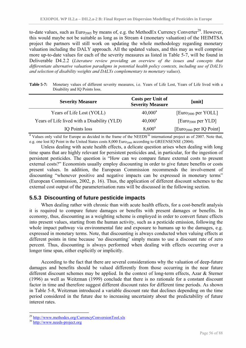
EXIOPOL WP II.2.a – DII.2.a-2 B: Final Report on Dispersion Modelling of Pesticides in Europe
Page 56 of 88
to-date values, such as Euro2005 by means of, e.g. the MethodEx Currency Converter29. However, this would maybe not be suitable as long as in Stream 4 (monetary valuation) of the HEIMTSA project the partners will still work on updating the whole methodology regarding monetary valuation including the DALY approach. All the updated values, and this may as well comprise more up-to-date values for each of the severity measures as listed in Table 5-7, will be found in Deliverable D4.2.2 (Literature review providing an overview of the issues and concepts that differentiate alternative valuation paradigms in potential health policy contexts, including use of DALYs and selection of disability weights and DALYs complementary to monetary values).
Table 5-7: Monetary values of different severity measures, i.e. Years of Life Lost, Years of Life lived with a
Disability and IQ Points loss.
Severity Measure Costs per Unit of Severity Measure [unit]
Years of Life Lost (YOLL) 40,000a [Euro2000 per YOLL] Years of Life lived with a Disability (YLD) 40,000a [Euro2000 per YLD]
IQ Points loss 8,600a [Euro2000 per IQ Point] a Values only valid for Europe as decided in the frame of the NEEDS30 international project as of 2007. Note that, e.g. one lost IQ Point in the United States costs 8,000 Euro2000 according to GREENSENSE (2004).
Unless dealing with acute health effects, a delicate question arises when dealing with long time spans that are highly relevant for persistent pesticides and, in particular, for the ingestion of persistent pesticides. The question is “How can we compare future external costs to present external costs?” Economists usually employ discounting in order to give future benefits or costs present values. In addition, the European Commission recommends the involvement of discounting “whenever positive and negative impacts can be expressed in monetary terms” (European Commission, 2002, p. 16). Thus, the application of different discount schemes to the external cost output of the parameterisation runs will be discussed in the following section.
5.5.3 Discounting of future pesticide impacts When dealing rather with chronic than with acute health effects, for a cost-benefit analysis
it is required to compare future damages or benefits with present damages or benefits. In economy, thus, discounting as a weighting scheme is employed in order to convert future effects into present values, starting from the human activity, such as a pesticide emission, following the whole impact pathway via environmental fate and exposure to humans up to the damages, e.g. expressed in monetary terms. Note, that discounting is always conducted when valuing effects at different points in time because ’no discounting’ simply means to use a discount rate of zero percent. Thus, discounting is always performed when dealing with effects occurring over a longer time span, either explicitly or implicitly.
According to the fact that there are several considerations why the valuation of deep-future
damages and benefits should be valued differently from those occurring in the near future different discount schemes may be applied. In the context of long-term effects, Azar & Sterner (1996) as well as Weitzman (1999) conclude that there is no rationale for a constant discount factor in time and therefore suggest different discount rates for different time periods. As shown in Table 5-8, Weitzman introduced a variable discount rate that declines depending on the time period considered in the future due to increasing uncertainty about the predictability of future interest rates.
29 http://www.methodex.org/CurrencyConversionTool.xls 30 http://www.needs-project.org

EXIOPOL WP II.2.a – DII.2.a-2 B: Final Report on Dispersion Modelling of Pesticides in Europe
Page 57 of 88
Table 5-8: Declining discount rate scheme suggested by Weitzman (1999) and particularly used within WSII.2 for human health damages via ingestion of persistent pesticides.
Time Horizon [years] Discount rates suggested by Weitzman (1999) 0-25 ‘low-normal’ real annual interest rate of around 3-4% 25-75 within-period instantaneous interest rate of around 2%
75-300 within-period instantaneous interest rate of around 1% > 300 within-period instantaneous interest rate of around 0%
When assuming 3.5% for the first 25 years according to Table 5-8, the resulting discount
factors for all years in the future are computed as shown in Table 5-9.
Table 5-9: Approach of calculating different discount factors for different time periods, as to be implemented particularly for the valuation of impacts of persistent pesticides via ingestion, according to Weitzman (1999).
Equation for calculating the discount factor Wt Equation is valid for the time period t
1(1 0.035)t tW =+
for: 0 25t< ≤
25 25
1 1(1 0.035) (1 0.02)t tW −= ⋅+ +
for: 25 75t< ≤
25 50 75
1 1 1(1 0.035) (1 0.02) (1 0.01)t tW −= ⋅ ⋅+ + +
for: 75 300t< ≤
25 50 225
1 1 1 1(1 0.035) (1 0.02) (1 0.01)tW = ⋅ ⋅ ⋅+ + +
for: 300t >
When dealing with comparing future effects or benefits to present effects or benefits via
the ingestion pathway it is necessary to distinguish between different parts of the whole chain, i.e. the time lag between the human activity, i.e. the emission of contaminants into environmental media, and a respective exposure as well as the time lag between the exposure and the corresponding physical impacts, such as a certain cancer. However, within the frame of EXIOPOL only the part between emission and exposure will be taken into consideration as part of the modelling approach by applying the steady-state solution to the environmental fate model, which can be seen as a ‘time-integrated exposure’ and thus as discounted exposure.
The calculation of the time-integrated exposure is further described in Bachmann (2006).
Steady-state is a situation in which no changes in concentration occur over time within a certain zone. This means that all outputs of a compartment in this zone, such as arable land, equal the inputs of this compartment in the same zone. Furthermore, Heijungs (1995) has shown that the steady-state situation can also be used for time-integrated exposure assessments of pulse emissions which are used for the present scenarios. When computing a time-integrated exposure as a kind of discounted exposure over time then a dynamic computation is not further required unless additional discount schemes are required to be used (Heijungs, 1995). However, as discounting is only relevant for persistent pesticides, it will be further discussed whether discounting will be considered at all when starting, e.g. with the estimation of externalities of currently used, mostly non-persistent pesticides within the scope of the EXIOPOL project.
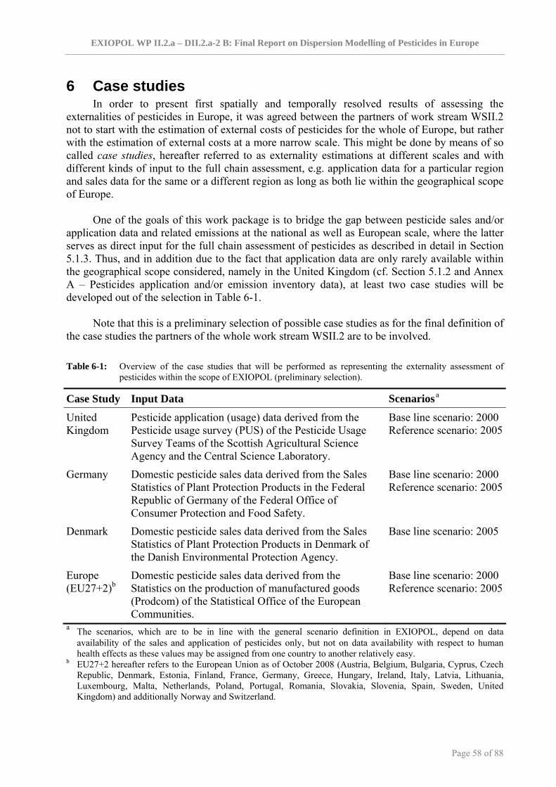
EXIOPOL WP II.2.a – DII.2.a-2 B: Final Report on Dispersion Modelling of Pesticides in Europe
Page 58 of 88
6 Case studies In order to present first spatially and temporally resolved results of assessing the
externalities of pesticides in Europe, it was agreed between the partners of work stream WSII.2 not to start with the estimation of external costs of pesticides for the whole of Europe, but rather with the estimation of external costs at a more narrow scale. This might be done by means of so called case studies, hereafter referred to as externality estimations at different scales and with different kinds of input to the full chain assessment, e.g. application data for a particular region and sales data for the same or a different region as long as both lie within the geographical scope of Europe.
One of the goals of this work package is to bridge the gap between pesticide sales and/or
application data and related emissions at the national as well as European scale, where the latter serves as direct input for the full chain assessment of pesticides as described in detail in Section 5.1.3. Thus, and in addition due to the fact that application data are only rarely available within the geographical scope considered, namely in the United Kingdom (cf. Section 5.1.2 and Annex A – Pesticides application and/or emission inventory data), at least two case studies will be developed out of the selection in Table 6-1.
Note that this is a preliminary selection of possible case studies as for the final definition of
the case studies the partners of the whole work stream WSII.2 are to be involved. Table 6-1: Overview of the case studies that will be performed as representing the externality assessment of
pesticides within the scope of EXIOPOL (preliminary selection).
Case Study Input Data Scenarios a
United Kingdom
Pesticide application (usage) data derived from the Pesticide usage survey (PUS) of the Pesticide Usage Survey Teams of the Scottish Agricultural Science Agency and the Central Science Laboratory.
Base line scenario: 2000 Reference scenario: 2005
Germany Domestic pesticide sales data derived from the Sales Statistics of Plant Protection Products in the Federal Republic of Germany of the Federal Office of Consumer Protection and Food Safety.
Base line scenario: 2000 Reference scenario: 2005
Denmark Domestic pesticide sales data derived from the Sales Statistics of Plant Protection Products in Denmark of the Danish Environmental Protection Agency.
Base line scenario: 2005
Europe (EU27+2)b
Domestic pesticide sales data derived from the Statistics on the production of manufactured goods (Prodcom) of the Statistical Office of the European Communities.
Base line scenario: 2000 Reference scenario: 2005
a The scenarios, which are to be in line with the general scenario definition in EXIOPOL, depend on data availability of the sales and application of pesticides only, but not on data availability with respect to human health effects as these values may be assigned from one country to another relatively easy.
b EU27+2 hereafter refers to the European Union as of October 2008 (Austria, Belgium, Bulgaria, Cyprus, Czech Republic, Denmark, Estonia, Finland, France, Germany, Greece, Hungary, Ireland, Italy, Latvia, Lithuania, Luxembourg, Malta, Netherlands, Poland, Portugal, Romania, Slovakia, Slovenia, Spain, Sweden, United Kingdom) and additionally Norway and Switzerland.

EXIOPOL WP II.2.a – DII.2.a-2 B: Final Report on Dispersion Modelling of Pesticides in Europe
Page 59 of 88
So far, for externality assessments of pesticides at the national scale only United Kingdom (for application of pesticides) and Germany (for pesticides sales) provide data sets for both years 2000 and 2005 and, thus, meet the definitions for case study scenarios within EXIOPOL. Hence, these two countries may be selected for the two national case studies but this, however, has not been finally agreed yet. For an externality assessment of pesticides at the European scale it can, so far, be recommended to use the Prodcom data provided by the Statistical Office of the European Communities (Eurostat) as input for a European wide case study. This, again, has not been finally agreed yet and may change due to updates throughout the data sets as listed in Annex A – Pesticides application and/or emission inventory data.

EXIOPOL WP II.2.a – DII.2.a-2 B: Final Report on Dispersion Modelling of Pesticides in Europe
Page 60 of 88
References Adam O, Badot PM, Degiorgi F, Crini G (2008) Mixture toxicity assessment of wood
preservative pesticides in the freshwater amphipod Gammarus pulex (L.). Ecotoxicology and Environmental Safety. In Press.
Alavanja, M. C., Hoppin, J. A., & Kamel, F. (2004) Health effects of chronic pesticide exposure: Cancer and neurotoxicity. Annual Review of Public Health, 25, 155-197.
Alloway BJ, Ayres DC (1997) Chemical Principles of Environmental Pollution. 2nd edition. London, Chapman and Hall.
Arias-Estévez M, López-Periago E, Martínez-Carballo E, Simal-Gándara J, Mejuto J-C, García-Río L (2008) The mobility and degradation of pesticides in soils and the pollution of groundwater resources. Agriculture, Ecosystems and Environment 123(4): 247-260.
Azar C, Sterner T (1996) Discounting and distributional considerations in the context of global warming. Ecological Economics 19: 169-184.
Bachmann TM (2006) Hazardous Substances and Human Health: Exposure, Impact and External Cost Assessment at the European Scale. Amsterdam, Elsevier.
Benjey W (1993) Agricultural pesticide emissions associated with common crops in the United States. United States – Environmental Protection Agency. Technical Report EPA/600/A-93/065 (NTIS PB93173136). Washington, D.C.
Bennett DH, Margni MD, McKone TE, Jolliet O (2002) Intake Fraction for Multimedia Pollutants: A Tool for Life Cycle Analysis and Comparative Risk Assessment. Risk Analysis 22: 903-916.
Bickel P, Friedrich R, eds. (2005) ExternE, Externalities of Energy Methodology 2005 Update. Brussels, European Commission.
Birkved M, Hauschild MZ (2006) PestLCI – A model for estimating field emissions of pesticides in agricultural LCA. Ecological Modelling 198(3-4): 433-451.
Bliefert C (2002) Umweltchemie. 3rd edition. Weinheim, Wiley-VCH.
Boethling RS, Howard PH, Meylan WM (2004) Finding and estimating chemical property data for environmental assessment. Environmental Toxicology and Chemistry 23(10): 2290-2308.
Boone MD (2008) Examining the single and interactive effects of three insecticides on amphibian metamorphosis. Environmental Toxicology and Chemistry 27(7):1561–1568.
Cedergreen N, Christensen AM, Kamper A, Kudsk P, Mathiassen SK, Streibig JC, Sørensen H (2008) A Review of Independent Action compared to Concentration Assition as Reference Models for Mixtures of Compounds with different Molecular Target Sites. Environmental Toxicology and Chemistry 27(7):1621–1632.
Crettaz P, Pennington DW, Rhomberg L, Brand K, Jolliet O (2002) Assessing Human Health in Life Cycle Assessment using ED10 s and DALYs: Part 1 - Cancer effects. Risk Analysis 22: 931-946.
de Jong FMW, de Snoo GR, van der Zande JC (2008) Estimated nationwide effects of pesticide spray drift on terrestrial habitats in the Netherlands. Journal of Environmental Management 86(4): 721-730.

EXIOPOL WP II.2.a – DII.2.a-2 B: Final Report on Dispersion Modelling of Pesticides in Europe
Page 61 of 88
Drever JI (1997) Catchment mass balance. In: Saether OM, de Caritat P (eds.) Geochemical processes, weathering and groundwater recharge in catchments. Balkema, Rotterdam, pp. 241-261.
Economopoulos AP (1993) Assessment of Sources of Air, Water, and Land Pollution. A Guide to Rapid Source Inventory Techniques and their use in Formulating Environmental Control Strategies. Part One: Rapid Inventory Techniques in Environmental Pollution. World Health Organisation, Geneva, Switzerland.
European Centre for Health Policy (1999) Health Impact Assessment: Gothenburg Consensus Paper. WHO, Brussels.
European Commission (1999) Externalities of Fuel Cycles - ExternE Project. Vol. 7 – Methodology (2nd edition). European Commission DG XII, Science Research and Development, JOULE, Brussels - Luxembourg.
European Commission (2002) Communication from the Commission on impact assessment. Commission of the European Communities, Brussels.
European Commission (2003) An applied integrated environmental impact assessment framework for the European Union (GREENSENSE). Brussels, European Commission.
European Environment Agency (2007) EMEP/CORINAIR Emission Inventory Guidebook – 2007. Prepared by the UNECE/EMEP Task Force on Emissions Inventories and Projections. European Environment Agency, Technical Report No 16/2007. Copenhagen.
Fauser P, Thomsen M, Sørensen PB, Petersen S (2008) Predicted Concentrations for Pesticides in Drainage Dominated Catchments. Water, Air & Soil Pollution 187(1-4): 149-156.
Fenner K, Scheringer M, MacLeod M, Matthies M, McKone T, Stroebe M, Beyer A, Bonnell M, Gall ACL, Klasmeier J, Mackay D, van de Meent D, Pennington D, Scharenberg B, Suzuki N, Wania F (2005) Comparing Estimates of Persistence and Long-Range Transport Potential among Multimedia Models. Environmental Science and Technology 39(7): 1932-1942.
Finizio A, Calliera M, Vighi M (2001) Rating Systems for Pesticide Risk Classification on Different Ecosystems. Ecotoxicology and Environmental Safety 49(3): 262-274.
Gallo MA, Lawryk NJ (1991) Organic phosphorus pesticides. In Hayes WJ, Laws ER (eds.) Handbook of pesticide toxicology. Academic Press, San Diego, California.
Geisz HN, Dickhut RM, Cochran MA, Fraser WR, Ducklow HW (2008) Melting Glaciers: A Probable Source of DDT to the Antarctic Marine Ecosystem. Environmental Science & Technology 42(11): 3958-3962.
Gold, LS, Stern, BR, Slone, TH, Brown, JP, Manley, NB, Ames, B (1997) Pesticide residues in food: investigation of disparities in cancer risk estimates, Cancer Letters 117: 195-207.
Gramatica P, Papa E, Francesca B (2004) Ranking and classification of non-ionic organic pesticides for environmental distribution: a QSAR approach. International Journal of Environmental Analytical Chemistry 84(1-3): 65-74.
GREENSENSE (2004) Final report on the GREENSENSE project to DG Research of the European Commission.
Hamilton D, Crossley S (2004) Pesticide Residues in Food and Drinking Water: Human Exposure and Risks. Chichester, John Wiley & Sons, Inc.
EXIOPOL WP II.2.a – DII.2.a-2 B: Final Report on Dispersion Modelling of Pesticides in Europe
Page 62 of 88
Hauschild M, Potting J (2003) Spatial differentiation in life cycle impact assessment - the EDIP2000 methodology. Department of Manufacturing Engineering and Management, Technical University of Denmark, Lyngby.
Hayes TB, Case P, Chui S, Chung D, Haeffele C, Haston K, Lee M, Mai VP, Marjuoa Y, Parker J, Tsui M (2006) Pesticide mixtures, endocrine disruption, and amphibian declines: are we underestimating the impact? Environmental Health Perspectives 114(S-1): 40-50.
Herbert BMJ, Halsall CJ, Villa S, Jones KC, Kallenborn R (2005) Rapid Changes in PCB and OC Pesticide Concentrations in Arctic Snow. Environmental Science & Technology 39(9): 2998-3005.
Heijungs R (1995) Harmonization of methods for impact assessment. Environmental Science & Pollution Research 2: 217-224.
Huijsmans JFM (1995) MJP-G Emissie-evaluatie 1995. Achtergronddocument (Scientific report). Commissie van Deskundigen, Institute of Agricultural and Environmental Engineering. Ministerie van LNV/IKC-L, pp. 127.
Humbert S, Margni M, Charles R, Salazar OMT, Quirós AL, Jolliet O (2007) Toxicity assessment of the main pesticides used in Costa Rica. Agriculture, Ecosystems & Environment 118(1-4): 183-190.
Hung H, Halsall CJ, Blanchard P, Li HH, Fellin P, Stern G, Rosenberg B (2002) Temporal Trends of Organochlorine Pesticides in the Canadian Arctic Atmosphere. Environmental Science & Technology 36(5): 862-868.
Intergovernmental Panel on Climate Change (2006) 2006 IPCC Guidelines for National Greenhouse Gas Inventories. Prepared by the National Greenhouse Gas Inventories Programme, Eggleston H.S., Buendia L., Miwa K., Ngara T. and Tanabe K. (Eds.). Institute for Global Environmental Strategies – IGES, Japan.
Janssen LHJM, Olivier JGJ, van Amstel AR (1999) Comparison of CH4 emission inventory data and emission estimates from atmospheric transport models and concentration measurements. Environmental Science & Policy 2: 295-314.
Jolliet O (1998) Life cycle impact assessment of pesticides on human health and ecosystems. In: Ceuterik D (ed.) Life cycle assessment in agriculture, agro-industry and forestry. VITO, mol. Helsinki, Finland, 109-119.
Jones DL, Fudge JS, Battye B (2001) Top Down Procedure for Estimating Solvent Area Source Emissions. Contract No. 68-D-98-046, WA 308 and 408. United States – Environmental Protection Agency. Research Triangle Park, NC.
Juraske R (2007) Advances in Life Cycle Impact Assessment of Pesticides: Methodological Improvements and Experimental Studies (Dissertation). Department of Chemical Engineering. Tarragona, Universitat Rovira i Virgili.
Juraske R, Antón A, Castells F, Huijbregts MAJ (2007a) PestScreen: A screening approach for scoring and ranking pesticides by their environmental and toxicological concern." Environment International 33(7): 886-893.
Juraske R, Antón A, Castells F, Huijbregts MAJ (2007b) Human intake fractions of pesticides via greenhouse tomato consumption: Comparing model estimates with measurements for Captan. Chemosphere 67(6): 1102-1107.
Jury WA, Spencer WF, Farmer WJ (1983) Use of models for assessing relative volatility, mobility, and persistence of pesticides and other trace organics in soil systems. In: Saxena

EXIOPOL WP II.2.a – DII.2.a-2 B: Final Report on Dispersion Modelling of Pesticides in Europe
Page 63 of 88
J (Ed.) Hazard assessment of chemicals – current developments, Vol. 2, Academic Press, New York, 1-43.
Kemm J (2007) What is HIA and why might it be useful? In: Wismar M, Blau J, Ernst K, Figueras J (Eds.) The effectiveness of health impact assessment: Scope and limitations of supporting decision-making in Europe. World Health Organisation, Copenhagen.
Kemm J, Parry J (2004) What is HIA? In: Kemm J, Parry J, Palmer S (eds.) Health impact assessment: Concepts, theory, techniques and applications. Oxford, Oxford University Press.
Kirkby, MJ, Imeson AC, Bergkamp G, Cammeraat LH (1996) Scaling up processes and models from the field plot to the watershed and regional areas. Journal of Soil and Water Conservation 51(5): 391-396.
Krewitt W, Pennington DW, Olsen SI, Crettaz P, Jolliet O (2002) Indicators for human toxicity in Life-Cycle Impact Assessment. In: Udo de Haes HA, Finnveden G, Goedkoop M, Hauschild M, Hertwich EG, Hofstetter P, Jolliet O, Klöpffer W, Krewitt W, Lindeijer E, Müller-Wenk R, Olsen SI, Pennigton DW, Potting J and Steen B (eds.) Life-cycle impact assessment: striving towards best practice. Society of Environmental Toxicology and Chemistry (SETAC), Pensacola, Florida, pp 123-148.
Leach AW, Mumford JD (2008) Pesticide Environmental Accounting: A method for assessing the external costs of individual pesticide applications. Environmental Pollution 151: 139-147.
Li K, Chen LQ, Li EC, Zhou ZK (2007) Acute Toxicity of the Pesticides Chlorpyrifos and Atrazine to the Chinese Mitten-handed Crab, Eriocheir Sinensis. Bulletin of Environmental Contamination and Toxicology 77(6): 918-924.
Li YF, Macdonald RW (2005) Sources and pathways of selected organochlorine pesticides to the Arctic and the effect of pathway divergence on HCH trends in biota: a review. Science of The Total Environment 342(1-3) 87-106.
Li YF, Scholtz MT, Van Heyst BJ (2003) Global Gridded Emissions Inventories of Beta-Hexachlorocyclohexane. Environmental Science and Technology 37(16): 3493-3498.
Liess M, Brown C, Dohmen P, Duquesne S, Hart A, Heimbach F, Kreuger J, Lagadic L, Reinert W, Maund S, Streloke M, Tarazona J (2005) Effects of Pesticides in the Field. Proceedings, European Union and SETAC Europe Workshop, 21-24 October 2003, Le Croisic, France. SETAC Press, Brussels, Belgium.
Liess M, Schulz R (1999) Linking insecticide contamination and population response in an agricultural stream. Environmental Toxicology and Chemistry, 18(9): 1948-1955.
Linders J, Mensink H, Stephenson G, Wauscope D, Racke K (2000) Foliar interception and retention values after pesticide application. A proposal for standardized values for environmental risk assessment. Pure and Applied Chemistry 72(11): 2199–2218.
Lu C, Barr DB, Pearson MA, Waller, LA (2008) Dietary intake and its contribution to longitudinal organophosphorus pesticide exposure in urban/suburban children. Environmental Health Perspectives 116(4): 537-542.
Lydy M, Belden J, Wheelock C, Hammock B, Denton D (2004) Challenges in regulating pesticide mixtures. Ecology and Society 9(6): 1.
Mackay D, Shiu WY, Ma KC (1997) Illustrated handbook of physical-chemical properties and environmental fate for organic chemicals: Pesticide Chemicals. Boca Raton, Lewis Publishers.

EXIOPOL WP II.2.a – DII.2.a-2 B: Final Report on Dispersion Modelling of Pesticides in Europe
Page 64 of 88
Margni M, Jolliet O, Rossier D, Crettaz P (2002) Life cycle impact assessment of pesticides on human health and ecosystems. Agriculture, Ecosystems and Environment 93: 379-392.
Maroni & Fait (1993) Health effects in man from long-term exposure to pesticides. A review of the 1975-1991 literature. Toxicology: 78(1-3); 1-180.
Matthies M, Scheringer M (2001) Long-Range Transport in the Environment. Environmental Science and Pollution Research 8(3): 149.
Midwest Research Institute (1994) Emission Factor Documentation for AP-42 Section 9.2.2, Pesticide Application, EPA Contract No. 68-D2-0159, Midwest Research Institute, Kansas City.
National Research Council (1987) Regulating pesticides in food: The Delaney paradox, Wash. DC: National Academy Press.
Pacyna JM et al. (1999) Final report for Project POPCYCLING-Baltic. EU DGXII, Environment and Climate Program ENV4-CT96-0214. Available on CD-Rom including technical report, the emission and environmental databases as well as the POPCYCLING-Baltic model. NILU, P.O. Box 100, N-2027 Kjeller, Norway.
Parry J, Kemm J (2004) Future directions for HIA. In: Kemm J, Parry J, Palmer S (eds.) Health impact assessment: Concepts, theory, techniques and applications. Oxford, Oxford University Press.
Pennington DW, Crettaz P, Tauxe A, Rhomberg L, Brand K, Jolliet O (2002) Assessing Human Health in Life Cycle Assessment using ED10 s and DALYs: Part 2 – Non-cancer effects. Risk Analysis 22: 947-963.
Pesticide Residues Committee (2007) Annual Report of the Pesticide Residues Committee 2006, Pesticide Residues Committee. United Kingdom.
Petticrew M, Cummins S, Sparks L, Findlay A (2007) Validating health impact assessment: Prediction is difficult (especially about the future). Environmental Impact Assessment Review 27(1): 101-107.
Pimentel D, Acquay H, Biltonen M, Rice P, Silva M, Nelson J, Lipner V, Giordano S, Horowitz A, D’Amore M (1992) Environmental and economic costs of pesticide use. BioScience 42: 750-760.
Pimentel D (2005) Environmental and economic costs of the application of pesticides primarily in the United States. Environment, Development and Sustainability 7: 229-252.
Potting J, Hauschild M (2005): General Issues. In: Potting J, Hauschild M. (eds.) Background for spatial differentiation in life cycle impact assessment – the EDIP2003 methodology. Environmental project no. 996. Danish Environmental Protection Agency. Copenhagen.
Pretty JN, Brett C, Gee D, Hine RE, Mason CF, Morison JIL, Raven H, Rayment MD, van der Bilj G (2000) An assessment of the total external costs of UK agriculture. Agricultural Systems 65: 113-136.
Pretty JN, Brett C, Gee D, Hine R, Mason C, Morison JIL, Rayment M, van der Bilj G, Dobbs T (2001) Policy and practice: policy challenges and priorities for internalizing the externalities of modern agriculture. Journal of Environmental Planning and Management 44. 263-283.
Pretty JN, Waibel H (2005) Paying the price: the full cost of pesticides. In: Pretty JN (ed.) The Pesticide Detox. London, Earthscan, pp. 39-54.
EXIOPOL WP II.2.a – DII.2.a-2 B: Final Report on Dispersion Modelling of Pesticides in Europe
Page 65 of 88
Ritter L, Solomon KR, Forget J (2001) Persistent Organic Pollutants – An Assessment Report on: DDT – Aldrin – Dieldrin – Endrin – Chlordane – Heptachlor – Hexachlorobenzene – Mirex – Toxaphene, Polychlorinated Biphenyls, Dioxins and Furans. The International Programme on Chemical Safety (IPCS) within the framework of the Inter-Organization Programme for the Sound Management of Chemicals (IOMC).
Sala S, Vighi M (2008) GIS-based procedure for site-specific risk assessment of pesticides for aquatic ecosystems. Ecotoxicology and Environmental Safety 69(1): 1-12.
Sanborn M, Cole D, Kerr K, Vakil C, Sanin KH, Bassil K. (2004) Systematic Review of Pesticide Human Health Effects. The Ontario College of Family Physicians, Canada.
Schäfer R, Caquet T, Siimes K, Mueller, R, Lagadic L, Liess M (2007) Effects of pesticides on community structure and ecosystem functions in agricultural headwater streams of three biogeographical regions in Europe. Science of the Total Environment. 382(2-3): 272-285.
Scheyer A, Morville S, Mirabel P, Millet M (2007) Variability of atmospheric pesticide concentrations between urban and rural areas during intensive pesticide application. Atmospheric Environment 41(17): 3604-3618.
Scholtz MT, McMillan AC, Slama C, Li YF, Ting N, Davidson K (1997) Pesticide Emissions Modeling – Development of a North American Pesticide Emissions Inventory. Canadian Global Emissions Interpretation Centre. Mississauga, Ontario. Report No. CGEIC-1997-1. Unpublished internal company report.
Scholtz MT, Van Heyst BJ, Ivanoff A, Taylor A (1999) Global Pesticide Emission Modeling with GEIA. In: Modelling and Sources – A Workshop on Techniques and Associated Uncertainties in Quantifying the Origin and Long-Range Transport of Contaminants to the Arctic. Bergen, Norway.
Simcox NJ, Fenske RA, Wolz SA, Lee IC, Kalman DA (1995) Pesticides in household dust and soil: exposure pathways for children of agricultural families. Environmental Health Perspectives 103(12): 1126–1134.
Tegtmeier EM, Duffy MD (2004) External costs of agricultural production in the united states. International Journal of Agricultural Sustainability 2, 155-175.
United States – Environmental Protection Agency (1995) Compilation of Air Pollutant Emission Factors, Volume 1: Stationary Point and Area Sources. Fifth edition. AP-42. United States – Environmental Protection Agency, Office of Air Quality Planning and Standards. Research Triangle Park, NC.
United States – Environmental Protection Agency (1998) Human Health Risk Assessment Protocol for Hazardous Waste Combustion Facilities, U.S. EPA Multimedia Planning and Permitting Division Office of Solid Waste.
United States – Environmental Protection Agency (2001) Pesticide registration facts. Office of Pesticide Programs, United States – Environmental Protection Agency, Washington, D.C.
United States – Environmental Protection Agency (2001) Emission Inventory Improvement Program. EIIP Technical Report Series, Volumes 1 – 5. Prepared by Eastern Research Group, Inc., Morrisville, North Carolina, for the Point Sources Committee of the Emission Inventory Improvement Program and for Roy Huntley of the Emission Factor and Inventory Group, United States – Environmental Protection Agency.
United States – Environmental Protection Agency (2006) Detailed Procedures for Preparing Emissions Factors (Draft). Prepared by MACTEC Federal Programs, Inc. United States – Environmental Protection Agency, Office of Air Quality Planning and Standards
EXIOPOL WP II.2.a – DII.2.a-2 B: Final Report on Dispersion Modelling of Pesticides in Europe
Page 66 of 88
Emissions Monitoring and Analysis Division, Emissions Factors and Policy Applications Group, Research Triangle Park, NC.
van den Berg F, Kubiak R, Benjey WG, Majewski MS, Yates SR, Reeves GL, Smelt JH, v. d. Linden AMA (1999) Emission of Pesticides into the Air. Water, Air & Soil Pollution 115(1-4): 195-218.
van der Gon DHAC, van het Bolscher M, Visschedijk AJH, Zandveld PYJ (2005) Study to the effectiveness of the UNECE Heavy Metals Protocol and costs of possible additional measures. Phase I: Estimation of emission reduction resulting from the implementation of the HM Protocol. TNO-report B&O-A R 2005/193.
Vida P, Moretto A (2007) Pesticide exposure pathways among children of agricultural workers. Journal of Public Health 15(4): 289-299.
Weitzman ML (1999) Just keep discounting, but ... In: Portney PR and Weyant JP (eds.) Discounting and intergenerational equity. Resources for the Future, Washington, DC, pp 23-29.
World Health Organization (2005) The WHO Recommended Classification of Pesticides by Hazard and guidelines to classification 2004. Geneva.
Yao Y, Harner T, Blanchard P, Tuduri L, Waite D, Poissant L, Murphy C, Belzer W, Aulagnier F, Sverko E (2008) Pesticides in the Atmosphere Across Canadian Agricultural Regions. Environmental Science and Technology 42(16): 5931-5937.

EXIOPOL WP II.2.a – DII.2.a-2 B: Final Report on Dispersion Modelling of Pesticides in Europe
Page 67 of 88
Annex Annex A – Pesticides application and/or emission inventory data Annex A 1: (E-1) Environment Canada and Global Emissions Inventory Activities working
group, GEIA: Global Pesticides Release Database ..................................................................68
Annex A 2: (E-2) Meteorological Synthesizing Centre-East, MSC-East: Database on Expert Emissions used in EMEP models .............................................................................................69
Annex A 3: (E-3) European Environment Agency and European Commission: European Pollutant Emission Register, EPER..........................................................................................70
Annex A 4: (E-4) European Environment Agency and European Commission: European Pollutant Release and Transfer Register, PRTR.......................................................................71
Annex A 5: (S-1) Statistical Office of the European Communities, Eurostat: Agriculture and Environment – Sales of Pesticides / Prodcom – Statistics on the Production of Manufactured Goods 73
Annex A 6: (S-2) Statistics Division of the Food and Agriculture Organization of the United Nations, FAOstat: Pesticides Consumption .............................................................................74
Annex A 7: (S-3) Organisation for Economic Co-operation and Development, OECD: OECD Environmental Data Compendium 2008 – Agriculture: Consumption and trends in consumption of pesticides. .......................................................................................................76
Annex A 8: (S-4) Federal Office of Consumer Protection and Food Safety, BVL: Sales of Plant Protection Products in the Federal Republic of Germany...............................................78
Annex A 9: (S-5) Danish Environmental Protection Agency, MST: Sales Statistics of Plant Protection Products in Denmark...............................................................................................79
Annex A 10: (A-1) Pesticide Usage Survey Teams of the Scottish Agricultural Science Agency and the Central Science Laboratory, CSL: Pesticide Usage Statistics........................82
Annex A 11: Pesticides active ingredients in the FOOTPRINT Pesticide Properties Database, PPDB .......................................................................................................................84
Annex B – Human health effect information regarding pesticides Annex B 1: Review of pesticides health effects .......................................................................88

EXIOPOL WP II.2.a – DII.2.a-2 B: Final Report on Dispersion Modelling of Pesticides in Europe
Page 68 of 88
Annex A – Pesticides application and/or emission inventory data Annex A 1: (E-1) Environment Canada and Global Emissions Inventory Activities working group, GEIA: Global
Pesticides Release Database
Description: In recognition of the increasingly urgent needs of the national and international community for accurate and complete usage, emission and residue data for pesticides, the Modelling & Integration Research Division of Air Quality Research Branch, Meteorological Service of Canada (MSC), Environment Canada, established the Global Pesticides Release Database (GloPeRD). GloPeRD provides high-quality gridded emission and residue data of persistent organochlorine pesticides, such as HCH and Toxaphene, with different scales and resolutions. These datasets can be used by scientific, industrial, educational, and policy-making communities. This research is also a contribution to the Global Emissions Inventory Activity (GEIA), a component of the International Global Atmospheric Chemistry (IGAC) core project of the International Geosphere – Biosphere Program (IGBP). URL: http://www.msc.ec.gc.ca/data/gloperd/emission_e.cfm
Data for download: http://www.msc.ec.gc.ca/data/gloperd/DataCenter_e.cfm (Note that data are only available for downloading to registered users, however, registration is free.)
Example: for an extraction of the Environment Canada data see Figure Annex 1.
Figure Annex 1: World map of global gridded alpha-HCH emissions [treleased/yr/cell] for 1990 with 1° latitude by 1° longitude grid resolution (Environment Canada and Global Emissions Inventory Activities working group, GEIA).
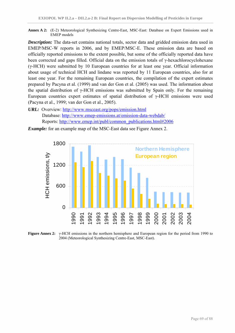
EXIOPOL WP II.2.a – DII.2.a-2 B: Final Report on Dispersion Modelling of Pesticides in Europe
Page 69 of 88
Annex A 2: (E-2) Meteorological Synthesizing Centre-East, MSC-East: Database on Expert Emissions used in EMEP models
Description: The data-set contains national totals, sector data and gridded emission data used in EMEP/MSC-W reports in 2006, and by EMEP/MSC-E. These emission data are based on officially reported emissions to the extent possible, but some of the officially reported data have been corrected and gaps filled. Official data on the emission totals of γ-hexachlorocyclohexane (γ-HCH) were submitted by 10 European countries for at least one year. Official information about usage of technical HCH and lindane was reported by 11 European countries, also for at least one year. For the remaining European countries, the compilation of the expert estimates prepared by Pacyna et al. (1999) and van der Gon et al. (2005) was used. The information about the spatial distribution of γ-HCH emissions was submitted by Spain only. For the remaining European countries expert estimates of spatial distribution of γ-HCH emissions were used (Pacyna et al., 1999; van der Gon et al., 2005). URL: Overview: http://www.msceast.org/pops/emission.html
Database: http://www.emep-emissions.at/emission-data-webdab/ Reports: http://www.emep.int/publ/common_publications.html#2006
Example: for an example map of the MSC-East data see Figure Annex 2.
0
600
1200
1800
1990
1991
1992
1993
1994
1995
1996
1997
1998
1999
2000
2001
2002
2003
2004
HC
H e
mis
sion
s, t/
y
Northern HemisphereEuropean region
Figure Annex 2: γ-HCH emissions in the northern hemisphere and European region for the period from 1990 to
2004 (Meteorological Synthesizing Centre-East, MSC-East).

EXIOPOL WP II.2.a – DII.2.a-2 B: Final Report on Dispersion Modelling of Pesticides in Europe
Page 70 of 88
Annex A 3: (E-3) European Environment Agency and European Commission: European Pollutant Emission Register, EPER
Description: EPER is the European Pollutant Emission Register, which was established by a Commission Decision of 17 July 2000. The EPER Decision is based on Article 15(3) of Council Directive 96/61/EC concerning integrated pollution prevention and control. According to the EPER Decision, Member States have to produce a triennial report on the emissions of industrial facilities into air and waters. The report covers 50 pollutants which must be included if the threshold values indicated in Annex A1 of the EPER Decision are exceeded. The first reporting year was 2001 (although Member States also had the option of providing data for 2000 and 2002). The second reporting year was 2004 and data were provided by the Member States in June 2006. For the third reporting year in 2007, EPER will be replaced by the European Pollutant Release and Transfer Register (European PRTR). Not all industrial plants existing are considered for EPER reporting – only those activities which are listed in Annex A3 of the EPER Decision are included. For the next reporting cycle, EPER will be integrated in the European Pollutant Release and Transfer Register (E-PRTR). The threshold values have been chosen in order to include about 90% of the emissions of the industrial facilities looked at, so as to prevent an unnecessarily high burden on all industrial facilities. Values indicated under ‘direct to water’ are emissions by facilities directly into the water environment. Values indicated under ‘indirect to water’ are releases by facilities via a sewer system into an off-site municipal or industrial waste water treatment plant. Since the pollution load is in general significantly reduced in these plants the values under ‘direct to water’ and ‘indirect to water’ should not be compared. URL: Data-set: http://eper.eea.europa.eu/eper/emissions_pollutants.asp Full Database: http://eper.eea.europa.eu/eper/files/EPER_dataset_27-03-2008.zip Further Information: http://eper.eea.europa.eu/eper/pollutant_list.asp#31 Example: for an extraction of the EPER data see Figure Annex 3.
Figure Annex 3: Aggregated emissions of Hexachlorocyclohexane to air and direct to water per industrial activity in which the emissions are generated in EU25 in 2004 (European Pollutant Emission Register, EPER).

EXIOPOL WP II.2.a – DII.2.a-2 B: Final Report on Dispersion Modelling of Pesticides in Europe
Page 71 of 88
Annex A 4: (E-4) European Environment Agency and European Commission: European Pollutant Release and Transfer Register, PRTR
Description: The European PRTR (E-PRTR) will implement at EU level the UNECE PRTR Protocol, which was signed by the European Community and 23 Member States in May 2003 in Kiev and which is a Protocol to the Aarhus Convention. The E-PRTR will succeed the European Pollutant Emission Register (EPER) under which data were reported for the years 2001 and 2004. The E-PRTR Regulation aims to enhance public access to environmental information through the establishment of a coherent and integrated E-PRTR, thereby finally also contributing to the prevention and reduction of pollution, delivering data for policy makers and facilitating public participation in environmental decision making. The Regulation establishes an integrated pollutant release and transfer register at Community level in the form of a publicly accessible electronic database and lays down rules for its functioning, in order to implement the UN-ECE Protocol on Pollutant Release and Transfer Registers and facilitate public participation in environmental decision making, as well as contributing to the prevention and reduction of pollution of the environment. The E-PRTR Regulation includes specific information on releases of pollutants to air, water and land and off-site transfers of waste and of pollutants in waste water. Those data have to be reported by operators of facilities carrying out specific activities31. In addition the E-PRTR includes data on releases from diffuse sources, e.g. road traffic and domestic heating, where such data is available.
URL: Data-sets: http://www.prtr.ec.europa.eu/ (available as from September 2009) Further Information - 1: http://www.home.prtr.de/index.php?pos=&lang=en Further Information - 2: http://www.eper.ec.europa.eu/eper/ Example: for an excerpt of the pollutants to be reported within the frame of the PRTR data see Table Annex 1. Table Annex 1: Pollutants to be reported according to the Guidance Document for the implementation of the
European PRTR as from 2007 (European Commission).
Threshold for releases (kg/year) No CAS number Pollutant(1) to air to water to land
25 15972-60-8 Alachlor - 1 1 26 309-00-2 Aldrin 1 1 1 27 1912-24-9 Atrazine - 1 1 28 57-74-9 Chlordane 1 1 1 29 143-50-0 Chlordecone 1 1 1 30 470-90-6 Chlorfenvinphos - 1 1 31 85535-84-8 Chloro-alkanes, C10-C13 - 1 1 32 2921-88-2 Chlorpyrifos - 1 1 33 50-29-3 DDT 1 1 1 34 107-06-2 1,2-dichloroethane (EDC) 1,000 10 10 35 75-09-2 Dichloromethane (DCM) 1,000 10 10 36 60-57-1 Dieldrin 1 1 1 37 330-54-1 Diuron - 1 1 38 115-29-7 Endosulphan - 1 1 39 72-20-8 Endrin 1 1 1
31 Only refers to activities as listed in Annex I of the Regulation (EC) No 166/2006 and, thus, will not include the agricultural sector (http://www.home.prtr.de/download/E-PRTR-VO_en.pdf).

EXIOPOL WP II.2.a – DII.2.a-2 B: Final Report on Dispersion Modelling of Pesticides in Europe
Page 72 of 88
Table Annex 1 (continued)
Threshold for releases (kg/year) No CAS number Pollutant(1) to air to water to land
40 - Halogenated organic compounds (as AOX)(2) - 1,000 1,000
41 76-44-8 Heptachlor 1 1 1 42 118-74-1 Hexachlorobenzene (HCB) 10 1 1 43 87-68-3 Hexachlorobutadiene (HCBD) - 1 1
44 608-73-1 1,2,3,4,5,6-hexachloro-cyclohexane (HCH) 10 1 1
45 58-89-9 Lindane 1 1 1 46 2385-85-5 Mirex 1 1 1
47 - PCDD + PCDF (dioxins + furans) (as Teq)(3) 0.0001 0.0001 0.0001
48 608-93-5 Pentachlorobenzene 1 1 1 49 87-86-5 Pentachlorophenol (PCP) 10 1 1
50 1336-36-3 Polychlorinated biphenyls (PCBs) 0.1 0.1 0.1
51 122-34-9 Simazine - 1 1 52 127-18-4 Tetrachloroethylene (PER) 2,000 10 - 53 56-23-5 Tetrachloromethane (TCM) 100 1 -
54 12002-48-1 Trichlorobenzenes (TCBs) (all isomers) 10 1 -
55 71-55-6 1,1,1-trichloroethane 100 - - 56 79-34-5 1,1,2,2-tetrachloroethane 50 - - 57 79-01-6 Trichloroethylene 2,000 10 - 58 67-66-3 Trichloromethane 500 10 - 59 8001-35-2 Toxaphene 1 1 1 60 75-01-4 Vinyl chloride 1,000 10 10
Notes: (1) Unless otherwise specified any pollutant specified in Annex II shall be reported as the total mass of that
pollutant or, where the pollutant is a group of substances, as the total mass of the group. (9) Halogenated organic compounds which can be adsorbed to activated carbon expressed as chloride. (10) Expressed as I-TEQ.

EXIOPOL WP II.2.a – DII.2.a-2 B: Final Report on Dispersion Modelling of Pesticides in Europe
Page 73 of 88
Annex A 5: (S-1) Statistical Office of the European Communities, Eurostat: Agriculture and Environment – Sales of Pesticides / Prodcom – Statistics on the Production of Manufactured Goods
Description: Eurostat presents data on sales of plant protection products communicated by Member States and some EFTA Countries to Eurostat on the basis of a so-called “gentlemen’s agreement”. In most countries, statistical offices or ministries of agriculture obtain data from national industries on a mandatory or voluntary base. Data refer to amounts of active ingredients, which are the substances in a commercial product that cause the desired effect on target organisms (weeds, pests, etc.) Most of the Member States refer to the definition of plant protection product given in Directive 91/414/EEC to delimit the scope of this indicator. Nevertheless there is no common definition adopted by all Member States and there can be significant differences in the range of products used in different countries, so that comparability is limited. The data stem from two special surveys made by ECPA, the European Crop Protection Association, among its ten full members, who claim to cover about 90% of the European market for plant protection products. The sources of the data were, in general, syndicated market research panels, e.g. annual farmer surveys carried out with a fairly constant target group. Data obtained from this representative user group were scaled up to national levels using common statistical methods. The crop types covered are identified as the key crop types accountable for the majority of the significant PPP applications in the EU (cereals, sugar beets, maize, oilseeds, potatoes, citrus, grapes, tree fruits and vegetables). URL: http://epp.eurostat.ec.europa.eu/pls/portal/url/page/SHARED/PER_AGRFIS
Further information (e.g. fruit and vegetable area by region and farm type): http://epp.eurostat.ec.europa.eu/portal/page?_pageid=3075,68081472&_dad=portal&_schema=PORTAL; Prodcom database: http://epp.eurostat.ec.europa.eu/portal/page?_pageid=2594,63266845&_dad=portal&_schema=PORTAL
Example: for an extraction of the Eurostat data see Table Annex 2. Table Annex 2: Total quantity of herbicides and insecticides [tactive ingredient/yr] sold in the EU15 Member States
for the years 1995, 2000 and 2005 (Statistical Office of the European Communities, Eurostat).
Sales of Herbicides Sales of Insecticides 1995 2000 2005 1995 2000 2005
Belgium 6,240 5,188 n.a. 1,115 925 n.a. Denmark 3,281 1,982 n.a. 163 41 n.a. Germany 16,065 16,610 14,699 861 846 977 Ireland 1,362 1,289 n.a. 108 60 n.a. Greece 2,131 2,331 n.a. 2,529 2,864 n.a. Spain 6,326 9,942 n.a. 9,538 10,470 n.a. France 27,416 31,500 n.a. 8,346 2,590 n.a. Italy 9,248 9,507 n.a. 4,651 7,135 n.a.
Luxembourg 164 n.a. n.a. 12 n.a. n.a. Netherlands 3,070 2,605 2,482 497 260 176
Austria 1,607 1,609 1,466 123 105 138 Portugal 1,660 1,826 1,751 397 476 425 Finland 791 862 n.a. 57 55 n.a. Sweden 975 1,364 1,280 17 17 18
United Kingdom 22,659 22,871 n.a. 1,171 661 n.a.
EXIOPOL WP II.2.a – DII.2.a-2 B: Final Report on Dispersion Modelling of Pesticides in Europe
Page 74 of 88
Annex A 6: (S-2) Statistics Division of the Food and Agriculture Organization of the United Nations, FAOstat: Pesticides Consumption
Description: The Statistics Division of the Food and Agriculture Organization of the United Nations started the collection of data on consumption of major individual pesticides products about three decades ago. However, the response to the related Pesticides Consumption Annual Questionnaire sent to all member countries was not very encouraging. Therefore, in 1986 in co-operation with the Commission of the European Union, a study was undertaken to find ways to improve the country coverage of the data. The present work of collecting data on groups of pesticides is a result of the recommendations of this study. Data collected earlier have been published in various issues of the Production Yearbook. The present database refers to the quantity of pesticides used in or sold to the agricultural sector expressed in metric tons of active ingredients. Information on quantities applied to single crops is not available. Data on consumption of pesticides are collected and presented for major groups and sub-groups as follows (only insecticides and herbicides will be shown as these are the two groups to be focussed within EXIOPOL):
• Insecticides: (a) chlorinated hydrocarbons, (b) organo-phosphates, (c) carbamates, (d) pyrethroids, (e) botanical and biological products, (f) others, not elsewhere classified.
• Herbicides: (a) phenoxy hormone products, (b) triazines, (c) amides, (d) Carbamates, (e) dinitroanilines, (f) urea derivatives, (g) sulfonyl ureas, (h) bipiridils, (i) uracil, (j) others not elsewhere classified.
A strict inter-country comparison on the basis of the database is not feasible because on the one hand the country coverage and time series are incomplete due to a high rate of non-response, and on the other hand although countries have been requested to report data in terms of active ingredients, some countries may have reported in formulation weight (including diluents and adjuvants) without specific indication. URL: http://faostat.fao.org/site/424/default.aspx
http://www.fao.org/ag/agp/agpp/pesticid/ (this link contains further Information about pesticide management which is an activity carried out within the overall framework of the Plant Protection Service of FAO)
Example: for an extraction of the FAOstat data see Table Annex 3.

EXIOPOL WP II.2.a – DII.2.a-2 B: Final Report on Dispersion Modelling of Pesticides in Europe
Page 75 of 88
Table Annex 3: Total quantity of herbicides and insecticides [tactive ingredient/yr] used in (or sold to) the agricultural sector (selection of European countries) for the years 1995 and 2000; data are generally expressed in terms of active ingredients (Statistics Division of the Food and Agriculture Organization of the United Nations, FAOstat).
Consumption of Herbicides Consumption of Insecticides 1995 2000 1995 2000 Austria 1,607 1,609 123 105 Belgium-Luxembourg n.a. n.a. n.a. n.a. Bulgaria n.a. n.a. n.a. n.a. Croatia 2,037 n.a. 204 n.a. Cyprus 122 n.a. 306 n.a. Czech Republic 2,461 2,613 101 147 Denmark 3,222 1,933 230 53 Estonia 109 285 2 3 Finland 815 863 51 51 France 27,419 31,500 8,848 2,590 Germany 16,065 16,610 1,518 1,281 Greece 1,883 2,331 1,696 2,864 Hungary 3,725 2,161 1,002 388 Ireland 1,362 1,289 106 53 Italy 27,165 9,432 40,874 8,859 Latvia 261 n.a. 3 n.a. Lithuania 573 482 5 7 Macedonia 169 n.a. 122 n.a. Malta 5 5 47 47 Netherlands 3,070 3,500 497 290 Norway 687 283 21 10 Poland 3,940 4,795 445 571 Portugal 1,659 1,827 396 476 Romania 8,147 3,869 3,624 1,239 Serbia and Montenegro 1,552 1,673 924 601 Slovakia 3,344 2,113 616 131 Slovenia 250 405 122 99 Spain 6,326 12,138 9,538 11,781 Sweden 975 1,372 32 22 Switzerland 657 653 95 96 Turkey 4,842 6,960 14,639 13,910 United Kingdom 22,753 22,900 1,667 1,681

EXIOPOL WP II.2.a – DII.2.a-2 B: Final Report on Dispersion Modelling of Pesticides in Europe
Page 76 of 88
Annex A 7: (S-3) Organisation for Economic Co-operation and Development, OECD: OECD Environmental Data Compendium 2008 – Agriculture: Consumption and trends in consumption of pesticides.
Description: The following tables show the state of and trends in the consumption of agricultural pesticides in selected countries. Pesticides are grouped into four categories: total pesticides, insecticides, fungicides and herbicides. There are additional data for “other pesticides”, which include fumigants, rodenticides and anti coagulants. State data are given for amounts of active ingredients, except for some countries where figures represent the pesticide formulations. “Active ingredients” are here the substances that cause the desired effects on agriculturally harmful fungi, plants or animals. Formulations, the product actually sold, contain both “active ingredients” and “inert” ingredients such as diluents and adjuvants. Trend data refer to pesticide consumption relative to a base year. When interpreting these tables, the reader should be extremely careful in making comparisons among countries and over time.
URL: Environmental data compendium: http://www.oecd.org/document/49/0,3343,en_2649_34283_39011377_1_1_1_1,00.html
Data-set: http://www.oecd.org/dataoecd/56/23/41255459.xls Example: for an extraction of the OECD data see Table Annex 4. Table Annex 4: Consumption of pesticides [tactive substance/yr](a,b); latest year available. (Source: Eurostat, FAO,
national statistical yearbooks, UNECE, UNEP, ECPA / Eurostat, FAO, annuaires statistiques nationaux, CEENU, PNUE, ECPA)
Country Year Insecticides Herbicides Country Year Insecticides Herbicides
Canada 2006 1,288 28,712 Hungary 2004 1,728 4,758
Mexico 2006 14,641 30,124 Iceland 2003 - 3
USA 2001 33,112 196,405 Ireland 2003 42 1,854
Japan 2006 22,554 12,016 Italy 2006 10,947 8,924
Australia 2006 8,036 24,789 Netherlands 2007 1,499 2,736
New Zealand 2007 299 3,077 Norway 2007 10 572
Austria 2005 274 1,466 Poland 2007 553 8,435
Belgium 2006 812 3,009 Portugal 2005 425 1,751
Czech Rep. 2006 182 2,639 Slovak Rep. 2006 222 1,413
Denmark 2006 57 2,479 Spain 2006 13,695 11,002
Finland 2006 40 1,274 Sweden 2007 54 1,809
France 2006 2,100 23,100 Switzerland 2006 105 595
Germany 2007 1,092 17,147 Turkey 2006 6,668 4,023
Greece 2006 2,540 2,250 UK 2006 1,075 12,284Notes: a) Unless otherwise specified, data refer to active ingredients. Insecticides: acaricides, molluscicides,
nematicides and mineral oils. Fungicides: bactericides and seed treatments. Herbicides: defoliants and desiccants. Other pesticides: plant growth regulators and rodenticides.
b) Data referring to sales or national production are an approximation of quantities in circulation; they cannot be considered as the volume actually used in a country, as certain amount of these volumes are still exported or stocked (for which exact data of these volumes are often unavailable).
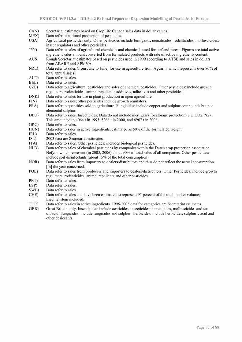
EXIOPOL WP II.2.a – DII.2.a-2 B: Final Report on Dispersion Modelling of Pesticides in Europe
Page 77 of 88
CAN) Secretariat estimates based on CropLife Canada sales data in dollar values. MEX) Data refer to national production of pesticides. USA) Agricultural pesticides only. Other pesticides include fumigants, nematicides, rodenticides, molluscicides,
insect regulators and other pesticides. JPN) Data refer to sales of agricultural chemicals and chemicals used for turf and forest. Figures are total active
ingredient sales amount converted from formulated products with rate of active ingredients content. AUS) Rough Secretariat estimates based on pesticides used in 1999 according to ATSE and sales in dollars
from ABARE and APMVA. NZL) Data refer to sales (from June to June) for use in agriculture from Agcarm, which represents over 80% of
total annual sales. AUT) Data refer to sales. BEL) Data refer to sales. CZE) Data refer to agricultural pesticides and sales of chemical pesticides. Other pesticides: include growth
regulators, rodenticides, animal repellents, additives, adhesives and other pesticides. DNK) Data refer to sales for use in plant production in open agriculture. FIN) Data refer to sales; other pesticides include growth regulators. FRA) Data refer to quantities sold to agriculture. Fungicides: include copper and sulphur compounds but not
elemental sulphur. DEU) Data refer to sales. Insecticides: Data do not include inert gases for storage protection (e.g. CO2, N2).
This amounted to 4064 t in 1995, 5266 t in 2000, and 6967 t in 2006. GRC) Data refer to sales. HUN) Data refer to sales in active ingredients, estimated as 50% of the formulated weight. IRL) Data refer to sales. ISL) 2003 data are Secretariat estimates. ITA) Data refer to sales. Other pesticides: includes biological pesticides. NLD) Data refer to sales of chemical pesticides by companies within the Dutch crop protection association
Nefyto, which represent (in 2005, 2006) about 90% of total sales of all companies. Other pesticides: include soil disinfectants (about 15% of the total consumption).
NOR) Data refer to sales from importers to dealers/distributors and thus do not reflect the actual consumption [in] the year concerned.
POL) Data refer to sales from producers and importers to dealers/distributors. Other Pesticides: include growth regulators, rodenticides, animal repellents and other pesticides.
PRT) Data refer to sales. ESP) Data refer to sales. SWE) Data refer to sales. CHE) Data refer to sales and have been estimated to represent 95 percent of the total market volume;
Liechtenstein included. TUR) Data refer to sales in active ingredients. 1996-2005 data for categories are Secretariat estimates. GBR) Great Britain only. Insecticides: include acaricides, insecticides, nematicides, molluscicides and tar
oil/acid. Fungicides: include fungicides and sulphur. Herbicides: include herbicides, sulphuric acid and other desiccants.

EXIOPOL WP II.2.a – DII.2.a-2 B: Final Report on Dispersion Modelling of Pesticides in Europe
Page 78 of 88
Annex A 8: (S-4) Federal Office of Consumer Protection and Food Safety, BVL: Sales of Plant Protection Products in the Federal Republic of Germany
Description: Data of domestic pesticide sales, parallel imports and exports for Germany can be obtained from the Federal Office of Consumer Protection and Food Safety (BVL). According to §19 of the national pesticide law (‘Pflanzenschutzmittelgesetz’), producers and retailers are obliged to inform the BVL about quantities of pesticides and active substances, respectively, sold within Germany and/or exported into other countries. The data in the online database are available on the basis of both a traded pesticide and an active substance. Pesticides sales data are grouped according to their intended purpose, e.g. insecticides. Data for active substances sales are, if required, available more detailed by breaking them down into target effect groups and chemical active substance classes, such as azoles and carbamates. The most recent publication of pesticides sales data is available for the year 2006; however, sales data for earlier years might be available upon request at the BVL. URL: Data-set:
http://www.bvl.bund.de/cln_007/DE/04__Pflanzenschutzmittel/01__ZulassungWirkstoffpruefung/01__Aktuelles/meld__par__19__Download,templateId=raw,property=publicationFile.pdf/meld_par_19_Download.pdf
Relation between trade products & active ingredients: https://portal.bvl.bund.de/psm/jsp/ Example: for an extraction of the BVL data see Table Annex 5. Table Annex 5: Development of domestic pesticide sales [tactive substance/yr] within Germany between 1998 and
2006 (Federal Office of Consumer Protection and Food Safety, BVL, 2007).
Active Substance Group 1998 2000 2002 2004 2006
Herbicides 17,269 16,610 14,328 15,923 17,015
Fungicides 10,530 9,641 10,129 8,176 10,251
Insecticides and Acaricides 6,276 6,111 5,889 7,328 7,780
without inert gases 1,037 845 742 1,082 813
inert gases 5,239 5,266 5,147 6,246 6,967
Other 4,808 3,232 4,332 3,704 3,740
Total 38,883 35,594 34,678 35,131 38,786
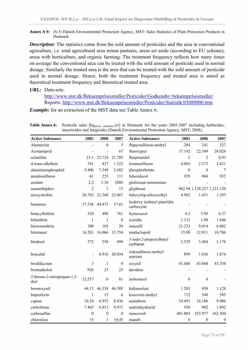
EXIOPOL WP II.2.a – DII.2.a-2 B: Final Report on Dispersion Modelling of Pesticides in Europe
Page 79 of 88
Annex A 9: (S-5) Danish Environmental Protection Agency, MST: Sales Statistics of Plant Protection Products in Denmark
Description: The statistics come from the sold amount of pesticides and the area in conventional agriculture, i.e. total agricultural area minus pastures, areas set aside (according to EU scheme), areas with horticulture, and organic farming. The treatment frequency reflects how many times on average the conventional area can be treated with the sold amount of pesticide used in normal dosage. Similarly the treated area is the area that can be treated with the sold amount of pesticide used in normal dosage. Hence, both the treatment frequency and treated area is stated as theoretical treatment frequency and theoretical treated area. URL: Data-sets:
http://www.mst.dk/Bekaempelsesmidler/Pesticider/Godkendte+bekæmpelsesmidler/ Reports: http://www.mst.dk/Bekaempelsesmidler/Pesticider/Statistik/03080000.htm Example: for an extraction of the MST data see Table Annex 6. Table Annex 6: Pesticide sales [kgactive substance/yr] in Denmark for the years 2005-2007 including herbicides,
insecticides and fungicides (Danish Environmental Protection Agency, MST, 2008).
Active Substance 2005 2006 2007 Active Substance 2005 2006 2007Abamectin - 0 5 flupyrsulfuron-methyl 284 241 327Acetamiprid - - 67 fluroxypyr 37.142 22.349 28.026aclonifen 23.1 23.724 21.705 flurprimidol 2 2 0,93d-trans-allethrin 741 427 1.323 foramsulfuron 4.065 2.373 2.621aluminiumphosphid 5.406 7.349 2.682 phosphorbrinte 0 0 7amidosulfuron 41 225 111 fuberidazol 929 968 932asulam 2.2 3.36 2880 glufosinat-ammonium - - -azamethiphos 2 1 13 glyphosat 962.94 1.128.327 1.231.120azoxystrobin 26.763 22.368 22.467 haloxyfop-ethoxyethyl 4.962 1.451 1.295
bentazon 37.538 44.873 37.61 hydroxy isobutyl piperidin carboxylat - - -
betacyfluthrin 320 496 761 hymexazol 4.2 5.95 6.37bifenthrin 1 1 0 icaridin 1.113 1.98 1.846bioresmethrin 100 103 20 imazalil 21.233 9.014 6.802bitertanol 16.201 16.066 15.754 imidacloprid 15.98 12.911 10.786
blodmel 372 558 498 3-iodo-2-propynylbutyl carbamat 3.529 3.484 3.178
boscalid - 8.916 20.054 iodosulfuron-methyl-natrium 899 1.036 1.074
brodifacoum 3 1 0 ioxynil 41.688 43.868 43.358bromadiolon 926 25 23 iprodion - - -
2-bromo-2-nitropropan-1,3-diol 32.557 0 81 isoborneol 0 0 -
bromoxynil 44.13 46.338 46.505 kaliumoleat 1.203 858 1.128buprofezin 1 15 6 kresoxim methyl 712 548 585captan 10.24 6.952 8.036 malathion 10.491 16.186 9.986carbofuran 7.465 6.013 9.971 maleinhydrazid 936 902 1.892carbosulfan 0 0 0 mancozeb 481.003 352.977 362.504chloralose 15 1 19,45 maneb 0 0 0
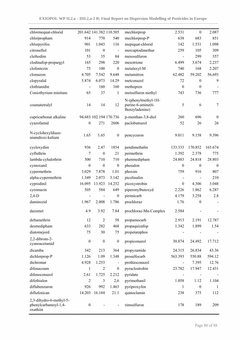
EXIOPOL WP II.2.a – DII.2.a-2 B: Final Report on Dispersion Modelling of Pesticides in Europe
Page 80 of 88
chlormequat-chlorid 201.642 141.382 110.505 mechlorprop 2.531 0 2.087chlorpropham 914 770 540 mechlorprop-P 638 683 851chlorpyrifos 901 1.043 116 mepiquat-chlorid 142 1.531 1.098citronellol 101 0 - mercaptodimethur 259 105 309clethodim 53 35 84 mesosulfuron - 299 357clodinafop-propargyl 165 298 220 mesotrione 6.499 3.674 2.237clofentezin 75 100 0 metalaxyl-M 740 168 2.207clomazon 4.705 7.542 9.648 metamitron 62.482 59.202 56.693clopyralid 5.874 6.073 14.29 metconazol 72 0 9clothianidin - 160 160 methopren 0 0 -Coniothyrium minitans 65 37 1 metsulfuron methyl 743 736 777
coumatetralyl 14 14 12N-(phenylmethyl-1H-purine-6-amine(6-Benzyladenine)
5 6 7
cupricarbonat alkaline 94.683 102.194 170.736 p-menthan-3,8-diol 260 696 0cyazofamid 0 271 2606 paclobutrazol 52 26 26
N-cyclohexyldiaze-niumdioxi-kalium 1.65 1.65 0 pencycuron 9.011 9.158 9.396
cycloxydim 936 2.47 1854 pendimethalin 133.333 170.852 165.674cyfluthrin 7 0 21 permethrin 1.392 2.378 775lambda-cyhalothrin 500 710 710 phenmedipham 24.883 24.818 28.803cymoxanil 0 0 0 phosalon 0 0 0cypermethrin 3.029 7.878 1.01 phoxim 759 916 807alpha-cypermethrin 1.349 2.073 3.142 picolinafen - - 210cyprodinil 16.095 13.923 14.252 picoxystrobin 0 4.306 3.048cyromazin 505 584 649 piperonylbutoxyd 2.226 1.862 6.2872,4-D - - 0 pirimicarb 4.179 3.258 2.8daminozid 1.967 2.008 1.786 prochloraz 1.76 0 -
dazomet 4.9 3.92 7.84 prochloraz-Mn-Complex 2.584 - -
deltamethrin 12 2 58 propamocarb 2.913 2.191 12.787desmedipham 633 282 468 propaquizafop 1.342 1.899 1.54diatomejord 75 30 75 propetamphos - - -
2,2-dibrom-2-cyanoacetamid 0 0 0 propiconazol 30.874 24.492 17.712
dicamba 342 213 364 propyzamide 24.315 26.834 43.36dichlorprop-P 1.126 1.09 1.348 prosulfocarb 563.393 550.88 594.12dichromat 4.928 1.253 - prothioconazol - 7.395 12.76difenacoum 1 2 0 pyraclostrobin 23.782 17.947 12.431difenoconazol 2.61 1.725 2.212 pyridate - - -difethialon 2 3 2,6 pyrimethanil 1.058 1.12 1.104diflubenzuron 926 992 1.463 pyriproxyfen 1 0 1diflufenican 14.203 16.184 21.1 quinoclamin 238 375 112
2,3-dihydro-6-methyl-5-phenylcarbamoyl-1,4-oxathiin
0 - - rimsulfuron 178 189 209

EXIOPOL WP II.2.a – DII.2.a-2 B: Final Report on Dispersion Modelling of Pesticides in Europe
Page 81 of 88
dimethoat 22.464 37.372 5.226 simazine - - -dimethomorph 188 200 246 spinosad 120 86 0
dinatrium-octaborat (natriumborat) 74 51 - spiroxamin 0 0 0
dinatrium-octaborat-tetrahydrat - 10.944 11.378 sulfosulfuron 392 445 381
dinatrium-tetraborat-decahydrat 0 0 0 tau-fluvalinat 8.836 9.536 9.459
diquat-dibromid 15.401 14.864 16.194 tebuconazol 26.227 21.76 26.708dithianon 2.233 3.073 3.178 teflubenzuron 72 0 0diuron 14.412 15.2 37.58 tefluthrin 500 375 255epoxiconazol 46.625 42.433 40.955 tepraloxidim 129 389 536esfenvalerat 58 73 81 terbuthylazin 91.607 38.106 34.594ethephon 22.557 12.154 53.992 thiamethoxam 666 385 578ethofumesat 12.754 9.078 8.097 thiophanat-methyl - - 452fenamidon - - 2.489 thiram 3.211 7.026 4.418fenazaquin 96 40 0 tolclofos-methyl 3.697 3.709 2.019fenhexamid 1.283 1.254 1.07 tolylfluanid 8.87 8.6 630fenoxaprop-P-ethyl 4.535 4.225 3.792 tralkoxydim - - 0fenpropidin 67.797 29.853 22.788 triasulfuron 0 0 0fenpropimorph 16.188 23.089 17.84 tribenuron-methyl 2.009 1.859 1.595fenpyroximat 50 64 43 triflumuron 7 0 40fipronil 4 2 6 trifluralin 242 232 144flamprop-M-isopropyl 0 - - triflusulfuron-methyl 586 547 479flocoumafen 0 0 0 triforin 282 - 435florasulam 432 397 510 trinexapac-ethyl 4.065 4.051 3.477fluazifop-P-butyl 5.865 4.528 3.137 ylang-ylangolie 6 0 4fluazinam 14.642 14.481 13.41 zoxamide - 0 46

EXIOPOL WP II.2.a – DII.2.a-2 B: Final Report on Dispersion Modelling of Pesticides in Europe
Page 82 of 88
Annex A 10: (A-1) Pesticide Usage Survey Teams of the Scottish Agricultural Science Agency and the Central Science Laboratory, CSL: Pesticide Usage Statistics
Description: This data-set contains data for 1990 onwards from the programme of pesticide usage surveys commissioned by the independent Advisory Committee on Pesticides. Data is collected by the Pesticide Usage Survey Teams at the Central Science Laboratory and the Scottish Agricultural Science Agency. Treated area is the gross area treated with a pesticide, including all repeat applications, some of which may have been applied to the land in preparation for drilling, or applied to a crop which subsequently failed and was re-drilled with the current crop, and thus may appear as an inappropriate use on that crop. Where quoted in the text, reasons for application are the farmer’s stated reasons for use of that particular pesticide on that crop and may not always seem entirely appropriate. Where individual active substances are mentioned in the text, they are listed in descending order of use by hectares treated. Throughout all tables, “Other” refers to chemicals grouped together because they were applied to less than 0.1% of the total area treated with pesticides. The term “formulation(s)” used within the text is used here to describe either single active substances or mixtures of active substances contained within an individual product. It does not refer to any of the solvents, pH modifiers or adjuvants also contained within a product that contribute to its efficacy. For the purposes of this survey arable crops include the following: wheat; winter barley; spring barley; oats; rye; triticale; oilseed rape; linseed; flax; ware potatoes; seed potatoes; peas for harvesting dry; field beans, sugar beet and other combinable crops including borage, hemp, lupines and poppies. Areas of set-aside land, which range from those sown or planted with industrial crops to those with natural regeneration, are included in this survey. All data are collected by personal interview using fully qualified staff working to standard operating procedures. Data are entered onto a computer database which has extensive error checking routines associated with the input program. Each item of data is then checked after entry and subsequently, all forms are re-checked by someone other than the original operator. Prior to compilation of the tables, the data are further subjected to a range of computer checks to detect, amongst other things, any values which, on agronomic grounds, appear suspect. Any thus revealed are further scrutinised, and, if necessary, referred back to the original source. URL: Data-set: http://pusstats.csl.gov.uk/
Pesticide usage survey reports: http://www.csl.gov.uk/newsAndResources/resourceLibrary/articles/puskm/
Example: for an extraction of the CSL data see Table Annex 7 and Table Annex 8.
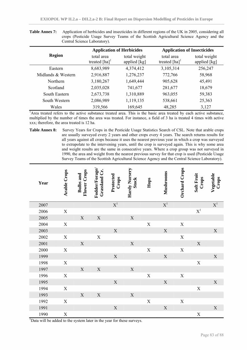
EXIOPOL WP II.2.a – DII.2.a-2 B: Final Report on Dispersion Modelling of Pesticides in Europe
Page 83 of 88
Table Annex 7: Application of herbicides and insecticides in different regions of the UK in 2005, considering all crops (Pesticide Usage Survey Teams of the Scottish Agricultural Science Agency and the Central Science Laboratory).
Application of Herbicides Application of Insecticides Region total area
treated [ha]1 total weight applied [kg]
total area treated [ha]1
total weight applied [kg]
Eastern 8,683,989 4,374,412 3,105,314 256,247 Midlands & Western 2,916,887 1,276,237 772,766 58,968
Northern 3,180,267 1,649,444 905,628 45,491 Scotland 2,035,028 741,677 281,677 18,679
South Eastern 2,673,738 1,310,889 963,055 59,383 South Western 2,086,989 1,119,135 538,661 25,363
Wales 319,566 169,645 48,285 3,127 1Area treated refers to the active substance treated area. This is the basic area treated by each active substance, multiplied by the number of times the area was treated. For instance, a field of 3 ha is treated 4 times with active xxx; therefore, the area treated is 12 ha.
Table Annex 8: Survey Years for Crops in the Pesticide Usage Statistics Search of CSL. Note that arable crops are usually surveyed every 2 years and other crops every 4 years. The search returns results for all years against all crops because it uses the nearest previous year in which a crop was surveyed to extrapolate to the intervening years, until the crop is surveyed again. This is why some area and weight results are the same in consecutive years. Where a crop group was not surveyed in 1990, the area and weight from the nearest previous survey for that crop is used (Pesticide Usage Survey Teams of the Scottish Agricultural Science Agency and the Central Science Laboratory).
Year
Ara
ble
Cro
ps
Bul
bs a
nd
Flow
er C
rops
Fodd
er/F
orag
e/
Gra
ssla
nd C
r.
Prot
ecte
d C
rops
Har
dy N
urse
ry
Stoc
k
Hop
s
Mus
hroo
ms
Orc
hard
Cro
ps
Soft
Fru
it C
rops
Veg
etab
le
Cro
ps
2007 X1 X1 X1 2006 X X1 2005 X X X 2004 X X X 2003 X X X 2002 X X X 2001 X X X 2000 X X X 1999 X X X 1998 X X 1997 X X X 1996 X X X 1995 X X X 1994 X X 1993 X X X 1992 X X X 1991 X X X 1990 X X
1Data will be added to the system later in the year for these surveys.

EXIOPOL WP II.2.a – DII.2.a-2 B: Final Report on Dispersion Modelling of Pesticides in Europe
Page 84 of 88
Annex A 11: Pesticides active ingredients in the FOOTPRINT Pesticide Properties Database, PPDB
Table Annex 9: List of pesticide active ingredients, comprising both pesticides that are still in use and pesticides that are not longer used within the EU, as addressed in the FOOTPRINT Pesticide Properties Database (PPDB) as of October 2008 32
1,2-benzisothiazolin-3-one coumachlor fosetyl-aluminium prohexadione-calcium 1,2-dichloropropane coumafuryl fosthiazate promecarb 1,3-dichloropropene coumaphos fuberidazole prometon 1-methylcyclopropene coumatetralyl furalaxyl prometryn 1-naphthylacetic acid crimidine furametpyr propachlor 2,3,6-TBA crotoxyphos furathiocarb propamocarb hydrochloride 2,4,5-trichlorophenol crufomate furfural propanil 2,4-D crystalline silica propaquizafop 2,4-DB cufraneb gamma-cyhalothrin propargite 2-aminobutane cyanamide gamma-HCH propazine 2-naphthyloxyacetic acid cyanazine gibberellic acid propetamphos 2-phenylphenol cyanophos glufosinate-ammonium propham 4-aminopyridine cyazofamid glyphosate trimesium propiconazole 4-CPA cyclanilide glyphosate propineb 6-benzylaminopurine cycloate gossyplure propionic acid 8-hydroxyquinoline sulfate cycloprothrin guazatine propoxur cyclosulfamuron propoxycarbazone-sodium abamectin cycloxydim halfenprox propyzamide acephate cycluron halofenozide proquinazid acequinocyl cyflufenamid halosulfuron-methyl prosulfocarb acetamiprid cyflumetofen haloxyfop prosulfuron acetic acid cyfluthrin haloxyfop-etotyl prothiocarb acetochlor cyhalofop-butyl haloxyfop-P prothioconazole acibenzolar-s-methyl cyhalothrin haloxyfop-P-methyl prothiofos acifluorfen cyhexatin heptachlor prothoate acifluorfen-sodium cymiazol heptenophos pymetrozine aclonifen cymoxanil hexachlorobenzene pyraclofos acrinathrin cypermethrin hexachlorophene pyraclonil acrolein cyphenothrin hexaconazole pyraclostrobin alachlor cyproconazole hexadecanoic acid pyraflufen-ethyl alanycarb cyprodinil hexaflumuron pyrasulfotole albendazole cyprofuram hexazinone pyrazophos aldicarb cyprosulfamide hexythiazox pyrazosulfuron-ethyl aldimorph cyromazine hydramethylnon pyrazoxyfen aldoxycarb hydrogen peroxide pyrethrins aldrin dalapon-sodium hydroprene pyribenzoxim allethrin daminozide hymexazol pyridaben allidochlor dazomet pyridafenthion alloxydim DDT icaridin pyridafol alpha-chlorohydrin deltamethrin imazalil pyridalyl alpha-cypermethrin demeton-S-methyl imazamethabenz-methyl pyridate alpha-naphthylthiourea desmedipham imazamox pyrifenox aluminium ammonium sulphate desmetryn imazapic pyrifluquinazon aluminium phosphide diafenthiuron imazapyr pyriftalid aluminium sulphate dialifos imazaquin pyrimethanil ametryn di-allate imazethapyr pyrimisulfan amicarbazone diazinon imazosulfuron pyriprole amidosulfuron dicamba imibenconazole pyriproxyfen aminocarb dichlobenil imicyafos pyrithiobac-sodium aminopyralid dichlofenthion imidacloprid pyroquilone amisulbrom dichlofluanid iminoctadine triacetate pyroxasulfone amitraz dichlone iminoctadine pyroxsulam amitrole dichlormid imiprothrin ammonium acetate dichlorobenzoic acid methylester indanofan quinalphos ammonium carbonate dichlorophen indolylacetic acid quinclorac ammonium hydroxide dichlorprop indoxacarb quinmerac ammonium sulphamate dichlorprop-P iodofenphos quinoclamine ammonium sulphate dichlorvos iodomethane quinoxyfen ammonium thiocyanate diclobutrazol iodosulfuron-methyl-sodium quintozene ampropylfos diclofop ioxynil octanoate quizalofop-ethyl
32 The FOOTPRINT Pesticide Properties Database (FOOTPRINT PPDB) is a comprehensive relational database of pesticide physicochemical and ecotoxicological data. The database has been developed by the Agriculture & Environment Research Unit (AERU) at the University of Hertfordshire, as part of the EU-funded FOOTPRINT project. The new database is a revised and greatly expanded version of the database that originally accompanied the Environmental Management for Agriculture software used in the UK. The database will be integrated in the FOOTPRINT pesticide risk assessment and management tools. (For further information please visit http://sitem.herts.ac.uk/aeru/footprint/)

EXIOPOL WP II.2.a – DII.2.a-2 B: Final Report on Dispersion Modelling of Pesticides in Europe
Page 85 of 88
ancymidol diclofop-methyl ioxynil quizalofop-P-ethyl anilazine diclomezine ipconazole quizalofop-P-tefuryl anilofos dicloran iprobenfos anthracene oil diclosulam iprodione resmethrin anthraquinone dicofol iprovalicarb rimsulfuron asulam sodium dicrotophos isazofos rotenone atrazine dicyclanil isobenzan aviglycine-HCl dicyclopentadiene isocarbophos sabadilla azaconazole dieldrin isofenphos-methyl saflufenacil azadirachtin dienochlor isopolinate scilliroside azafenidin diethofencarb isoprocarb secbumeton azamethiphos diethyltoluamide isopropalin sethoxydim azimsulfuron difenacoum isoprothiolane siduron azinphos-ethyl difenoconazole isoproturon silthiofam azinphos-methyl difenoxuron isotianil simazine aziprotryne difenzoquat isoval simeconazole azobenzene difethialone isoxaben simetryn azocyclotin diflovidazin isoxaflutole sintofen azoxystrobin diflubenzuron isoxathion S-metolachlor diflufenican sodium 5-nitroguaiacolate Bacillus sphaericus diflufenzopyr kaolin sodium carbonate Bacillus subtilis diflumetorim karbutilate sodium chlorate Bacillus thuringiensis dikegulac kasugamycin hydrochloride hydrate sodium chloride barban dikegulac-sodium kinoprene sodium o-nitrophenolate beflubutamid dimefox kresoxim-methyl sodium p-nitrophenolate benalaxyl dimefuron spinetoram benalaxyl-M dimepiperate lactofen spinosad benazolin ethyl dimethachlor lambda-cyhalothrin spirodiclofen benazolin dimethametryn laminarin spiromesifen bendiocarb dimethenamid L-carvone spirotetramat benfluralin dimethenamid-P lenacil spiroxamine benfuracarb dimethipin limonene sulcotrione benfuresate dimethirimol linuron sulfentrazone benodanil dimethoate lithium perfluorooctane sulfonate sulfluramid benomyl dimethomorph lufenuron sulfometuron-methyl benoxacor dimethylvinphos sulfosulfuron benquinox dimoxystrobin magnesium phosphide sulfotep bensulfuron-methyl diniconazole malathion sulphur bensulide dinitramine maleic hydrazide sulphuric acid bensultap dinobuton mancopper sulprofos bentaluron dinocap mancozeb bentazone dinoseb mandipropamid tau-fluvalinate benthiavalicarb dinotefuran maneb TCA-sodium benzalkonium chloride dinoterb MCPA TDE benzfendizone dioxacarb MCPA-thioethyl tebuconazole benzobicyclon dioxathion MCPB tebufenozide benzofenap diphacinone mecarbam tebufenpyrad benzoximate diphenamid mecoprop tebutam benzoylprop diphenylamine mecoprop-P tebuthiuron benzoylprop-ethyl diquat dibromide mefenacet tecloftalam benzthiazuron disulfoton mefenpyr tecnazene beta-cyfluthrin ditalimfos mefluidide teflubenzuron beta-cypermethrin dithianon menazon tefluthrin bifenazate dithiopyr mepanipyrim tembotrione bifenox diuron mephosfolan temephos bifenthrin DNOC mepiquat chloride tepraloxydim bilanafos dodemorph acetate mepronil terbacil bilanafos-sodium dodemorph meptyldinocap terbufos binapacryl dodine merphos terbumeton bioallethrin mesosulfuron-methyl terbuthylazine bioresmethrin edifenphos mesotrione terbutryn biphenyl emamectin benzoate metaflumizone tetrachlorvinphos bispyribac-sodium endosulfan metalaxyl tetraconazole bistrifluron endothal metalaxyl-M tetradifon bitertanol endothion metaldehyde tetraethyl pyrophosphate bixafen endrin metam tetramethrin blasticidin-S EPN metamitron tetrasul bone oil epoxiconazole metarhizium anisopliae thenylchlor Bordeaux mixture EPTC metazachlor thiabendazole boscalid esfenvalerate metconazole thiacloprid brodifacoum esprocarb methabenzthiazuron thiamethoxam bromacil etaconazole methamidophos thiazafluron bromadiolone ethaboxam methasulfocarb thiazopyr bromethalin ethalfluralin methazole thidiazuron bromobutide ethametsulfuron-methyl methfuroxam thiencarbazone-methyl bromocyclen ethanedial methidathion thifensulfuron-methyl bromofenoxim ethanethiol methiocarb thifluzamide

EXIOPOL WP II.2.a – DII.2.a-2 B: Final Report on Dispersion Modelling of Pesticides in Europe
Page 86 of 88
bromophos ethephon methomyl thiobencarb bromophos-ethyl ethidimuron methoprene thiocyclam hydrogen oxalate bromopropylate ethiofencarb methoxychlor thiocyclam bromoxynil heptanoate ethion methoxyfenozide thiodicarb bromoxynil octanoate ethiprole methyl bromide thiofanox bromoxynil ethirimol metiram thiometon bromuconazole ethofumesate metobromuron thionazin bronopol ethoprophos metofluthrin thiophanate-methyl bupirimate ethoxyquin metolachlor thiourea buprofezin ethoxysulfuron metominostrobin thiram butachlor etofenprox metosulam tiocarbazil butafenacil etoxazole metoxuron tolclofos-methyl butocarboxim etridiazole metrafenone tolylfluanid butoxycarboxim etrimfos metribuzin topramezone butralin metsulfuron-methyl tralkoxydim butroxydim famoxadone mevinphos tralomethrin buturon fatty acids mexacarbate transfluthrin butylate fenamidone milbemectin triadimefon fenaminosulf mirex triadimenol cadusafos fenamiphos molinate tri-allate cafenstrole fenarimol monalide triasulfuron calciferol fenazaflor monocrotophos triazamate calcium carbonate fenazaquin monolinuron triazophos calcium chloride fenbuconazole monuron triazoxide calcium hydroxide fenbutatin oxide MSMA tribenuron-methyl calcium phosphate fenchlorazole muscalure tribufos calcium phosphide fenchlorphos myclobutanil trichlorfon camphechlor fenclorim trichloronate captafol fenfuram nabam triclopyr captan fenhexamid naled tricyclazole carbaryl fenitrothion naphthalene tridemorph carbendazim fenobucarb naproanilide tridiphane carbetamide fenoprop napropamide trietazine carbofuran fenothiocarb naptalam trifloxystrobin carbon dioxide fenoxanil neburon trifloxysulfuron carbon tetrachloride fenoxaprop-ethyl nicosulfuron trifloxysulfuron-sodium carbophenothion fenoxaprop-P-ethyl nicotine triflumizole carbosulfan fenoxycarb nitralin triflumuron carboxin sulfoxide fenpiclonil nitrapyrin trifluralin carboxin fenpropathrin nitrothal isopropyl triflusulfuron-methyl carfentrazone-ethyl fenpropidin norbormide triforine carpropamid fenpropimorph norflurazon trimedlure cartap fenpyroximate noruron trimethacarb cetrimide fenson novaluron trinexapac-ethyl chinomethionat fensulfothion noviflumuron triticonazole chitosan fenthion nuarimol tritosulfuron chlomethoxyfen fentin acetate chloralose fentin hydroxide octhilinone uniconazole chloramben fentrazamide ofurace urea sulphate chloranil fenuron olein chlorantraniliprole fenvalerate omethoate validamycin chlorbenside ferbam orbencarb vamidothion chlorbromuron ferrous sulphate orthosulfamuron vernolate chlorbufam fipronil orysastrobin vinclozolin chlordane flamprop oryzalin chlordecone flamprop-M-isopropyl oxadiargyl warfarin chlordimeform flazasulfuron oxadiazon chlorethoxyfos flocoumafen oxadixyl XMC chlorfenac flonicamid oxamyl chlorfenapyr florasulam oxasulfuron zeta-cypermethrin chlorfenprop-methyl fluacrypyrim oxpoconazole fumarate zinc oxide chlorfenson fluazifop-butyl oxycarboxin zineb chlorfenvinphos fluazifop-P-butyl oxydemeton-methyl ziram chlorfluazuron fluazinam oxyfluorfen zoxamide chlorflurenol fluazolate oxytetracycline chloridazon flubendiamide Other product constituents chlorimuron-ethyl flubenzimine paclobutrazol chlormephos flucarbazone-sodium paraquat 1,1,1-acetonitrile chlormequat chloride fluchloralin parathion 1,2-benzisothiazolin-3-one chlorobenzilate flucycloxuron parathion-methyl 2-butoxyethanol chloroneb flucythrinate pebulate alcohol ethoxylate chlorophacinone fludioxonil pelargonic acid bentonite chlorophyllin flufenacet penconazole butan-1-ol chloropicrin flufenoxuron pencycuron butyl stearate chloropropylate flufenzin pendimethalin calcium carbonate chlorothalonil flumetralin penoxsulam carbon tetrachloride chlorotoluron flumetsulam pentachlorophenol citric acid anhydrous
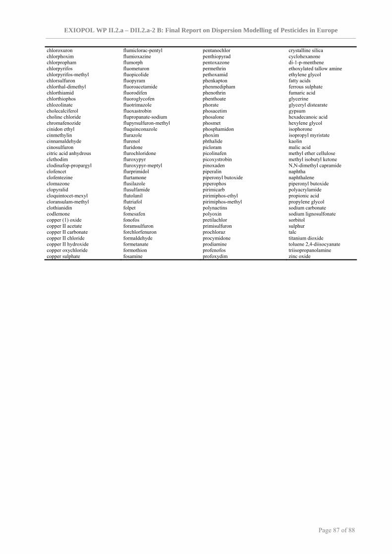
EXIOPOL WP II.2.a – DII.2.a-2 B: Final Report on Dispersion Modelling of Pesticides in Europe
Page 87 of 88
chloroxuron flumiclorac-pentyl pentanochlor crystalline silica chlorphoxim flumioxazine penthiopyrad cyclohexanone chlorpropham flumorph pentoxazone di-1-p-menthene chlorpyrifos fluometuron permethrin ethoxylated tallow amine chlorpyrifos-methyl fluopicolide pethoxamid ethylene glycol chlorsulfuron fluopyram phenkapton fatty acids chlorthal-dimethyl fluoroacetamide phenmedipham ferrous sulphate chlorthiamid fluorodifen phenothrin fumaric acid chlorthiophos fluoroglycofen phenthoate glycerine chlozolinate fluotrimazole phorate glyceryl distearate cholecalciferol fluoxastrobin phosacetim gypsum choline chloride flupropanate-sodium phosalone hexadecanoic acid chromafenozide flupyrsulfuron-methyl phosmet hexylene glycol cinidon ethyl fluquinconazole phosphamidon isophorone cinmethylin flurazole phoxim isopropyl myristate cinnamaldehyde flurenol phthalide kaolin cinosulfuron fluridone picloram malic acid citric acid anhydrous flurochloridone picolinafen methyl ether cellulose clethodim fluroxypyr picoxystrobin methyl isobutyl ketone clodinafop-propargyl fluroxypyr-meptyl pinoxaden N,N-dimethyl capramide clofencet flurprimidol piperalin naphtha clofentezine flurtamone piperonyl butoxide naphthalene clomazone flusilazole piperophos piperonyl butoxide clopyralid flusulfamide pirimicarb polyacrylamide cloquintocet-mexyl flutolanil pirimiphos-ethyl propionic acid cloransulam-methyl flutriafol pirimiphos-methyl propylene glycol clothianidin folpet polynactins sodium carbonate codlemone fomesafen polyoxin sodium lignosulfonate copper (1) oxide fonofos pretilachlor sorbitol copper II acetate foramsulfuron primisulfuron sulphur copper II carbonate forchlorfenuron prochloraz talc copper II chloride formaldehyde procymidone titanium dioxide copper II hydroxide formetanate prodiamine toluene 2,4-diisocyanate copper oxychloride formothion profenofos triisopropanolamine copper sulphate fosamine profoxydim zinc oxide

EXIOPOL WP II.2.a – DII.2.a-2 B: Final Report on Dispersion Modelling of Pesticides in Europe
Page 88 of 88
Annex B – Human health effect information regarding pesticides Annex B 1: Review of pesticides health effects
The table below summarises the information regardeing health effect of pesticides available from the reviews consulted (Maroni and Fait, 1993; Alvanja et al, 2004; Sanborn et al, 2004; plus confidential material from an ongoing study not yet published). Many of the reviews were not specific about which pesticide was implicated in the exposure. More recent studies were more likely to show relationships than earlier ones, either because more effort had gone into exposure assessment or because earlier studies had been revisited with longer follow-up periods. Table Annex 10: Summary of health effects identified, quantified or rejected on the basis of epidemiological
studies in humans.
brai
n ca
ncer
brea
st c
ance
r
kidn
ey c
ance
r
lung
can
cer
ovar
ian
canc
er
panc
reat
ic c
ance
r
pros
tate
can
cer
stom
ach
canc
er
NH
L
Leuk
aem
ia
Gen
otox
icity
or
Imm
unot
oxic
ity
Der
mat
olog
ic e
ffec
ts
neur
olog
ical
& m
enta
l he
alth
impa
cts
Rep
rodu
ctiv
e ou
tcom
es
Organochlorine q q
Organophosphate q
Carbamate q
Pyrethroids Inse
ctic
ides
Insecticides q q
Phenoxyacetic Acid q
Triazine q q Bipyridilium H
erbi
cide
s
Herbicides q
PESTICIDES q x;q q q q x;q q q q
Arsenical pesticides q
KEY: Evidence of no relation x Evidence of relation Quantitative evidence of relation q