1

Direct-to-Indirect Acoustic RadianceTransfer

Lakulish Antani, Anish Chandak, Micah Taylor and Dinesh ManochaTR10-012

Abstract—We present an efficient algorithm for simulating diffuse reflections of sound in a static scene. Ourapproach is built on the latest advances in precomputed light transport techniques for visual rendering and usesthem to develop an improved acoustic radiance transfer technique. We precompute a direct-to-indirect acoustictransfer operator for the scene, and use it to map direct sound incident on the surfaces of the scene to multi-bounce diffuse indirect sound, which is then gathered at the listener to compute the final impulse response. Ouralgorithm decouples the transfer operator from the source position so we can efficiently update the acousticresponse at the listener when the source moves. We highlight its performance on various benchmarks andobserve significant speedups over prior methods based on acoustic radiance transfer.

Index Terms—sound propagation, radiosity, virtual reality, precomputed transport

F

1 INTRODUCTION

Sound rendering or auditory displays can aug-ment graphical rendering and provide the userwith an enhanced spatial sense of presence.Some of the driving applications of sound ren-dering include acoustic design of architecturalmodels or outdoor scenes, walkthroughs oflarge CAD models with sounds of machineparts or moving people, urban scenes withtraffic, computer games, etc. The computationof sound propagation paths takes into accountthe knowledge of sound sources, listener loca-tions, the 3D model of the environment, andmaterial absorption and scattering properties.

The modeling of sound propagation effectsneeds to account for different wave propa-gation phenomena such as specular reflec-tions, scattering (including diffuse reflectionsand edge diffraction), interference, etc. In thispaper, we mainly focus on the modeling ofdiffuse reflections, which are considered im-portant for modeling sound propagation [1].Many objective [2] and perceptual [3] studieshave been conducted to ascertain the impor-tance of diffuse reflections for sound propaga-tion. Further, it is computationally challengingto model high orders of diffuse reflection.Thus, due to its importance and computa-tional challenge, modeling diffuse reflectionsfor sound propagation is an active area of

interest in many sound rendering applications.At a broad level, sound propagation

algorithms can be classified into numericaland geometric methods. Numerical methodsattempt to directly compute numericalsolutions to the acoustic wave equation.However, the complexity of these methods isproportional to the volume of the scene andthe fourth power of the maximum frequencyof sound simulated, and can be very slowfor large acoustic spaces or high frequencysound sources. In terms of geometric soundpropagation, two standard methods used tosimulate diffuse sound reflections are basedon ray (or volume) tracing and radiancetransfer. Our approach is motivated by recentdevelopments in global illumination based onprecomputed light transport algorithms [4],[5], [6]. Specifically, our work is inspired bydirect-to-indirect transfer algorithms for visualrendering, that map direct light incident onthe surfaces of a scene to indirect light on thesurfaces of the scene after multiple bounces.

Main Results We present a new algorithm formodeling diffuse reflections of sound based onthe direct-to-indirect transfer approach. Thisformulation decouples the precomputation ofacoustic radiance transfer operators from boththe source and the listener positions, and canefficiently update the acoustic response at the

2

listener whenever the source moves.The algorithm uses an SVD approximation

of the transfer operator to perform higher-order diffuse reflections. We show that thisallows us to reduce the memory requirementsand increase the performance of our algo-rithm. Our algorithm decouples the transferoperator from the source position, and thusaccelerates the computations as compared tothe state-of-the-art.

We highlight the performance of ouralgorithm on various models. In practice,it is much faster than prior methods basedon radiance transfer. To the best of ourknowledge, it is the first approach that canperform diffuse reflections in static sceneswith moving sources at almost interactiverates.

The rest of this paper is organized as fol-lows. Section 2 covers some background ma-terial and gives a brief survey of relatedwork. Section 3 gives a broad overview of ourapproach. Section 4 discusses our direct-to-indirect acoustic radiance transfer algorithm,and we describe its implementation in Sec-tion 5. Section 6 presents some experimentalresults and compares the performance of ouralgorithm with prior methods.

2 RELATED WORK

In this section, we give a brief overviewof prior algorithms for radiance transfercomputation and diffuse reflections.

Numerical Acoustics The propagationof sound in a medium is governed by theacoustic wave equation, a second-order partialdifferential equation [7]. Several techniques(e.g., finite difference time-domain method)are known for directly solving the waveequation using numerical methods [8], [9]and accurately modeling sound propagationin a scene. Modeling diffuse reflections isessentially a matter of specifying appropriateboundary conditions to the numerical solverand performing the simulation on a grid fineenough to capture the detailed “roughness”of the surfaces that results in acoustic wavescattering [10]. However, despite recentadvances [9], these methods can be ratherslow and are mainly limited to simple static

sources. Precomputation-based methods haverecently been developed [11] that use anumerical simulator to compute the acousticresponse of a scene from several sampledsource positions; at runtime these responsesare interpolated given the actual sourceposition. These methods are fast, but requirelarge amounts of precomputed data.

Geometric Acoustics Most sound propaga-tion techniques used in practical applicationsmodel the acoustic effects of an environ-ment in terms of linearly propagating rays or3D volumes. These geometric acoustics tech-niques are not as accurate as numerical meth-ods in terms of solving the wave equation, andcannot easily model all kinds of propagationeffects, but allow efficient simulation of earlyreflections.

Methods based on ray tracing [12], [13]are able to model both diffuse and specularreflections of sound. Since early specularreflections provide the listener with importantperceptual cues regarding the direction ofsound, specialized techniques have beendeveloped for modeling specular reflections,which include volume tracing [14], [15] andthe image source method [16], [17]. For staticscenes, which frequently arise in architecturalacoustics and virtual environments, radiancetransfer methods can be used to simulatereflections from surfaces with arbitrary BRDFs[18], [19]. Many techniques have also beendesigned to simulate edge diffraction [20],[21], [22].

Precomputed Light Transport The radiosityalgorithm [23] is the classic example of analgorithm which precomputes light transporteffects in a scene. However, the classic radios-ity algorithm uses a full solution that needsto be recomputed every time the light sourcemoves. In contrast, precomputed radiance trans-fer (PRT) algorithms essentially decouple lighttransport effects from the light source con-figuration. This is performed by computinga linear operator that defines how a variablelight source configuration affects the radiancesat sample points on the surfaces in the scene.PRT techniques can support both distant [4],[24] and local [25] source configurations.

Direct-to-indirect transfer algorithms [5], [6]

3

are one class of precomputed light transportalgorithms. These algorithms compute linearoperators which map direct light incident onthe surface samples to multi-bounce indirectlight at the samples. These algorithms are de-signed to handle diffuse reflections, and someof them can also support limited glossy reflec-tions. In order to reduce the storage and pro-cessing requirements, these techniques projectthe radiance function over the surface of thescene into a hierarchical basis, such as Haarwavelets [26] or the spectral mesh basis [27].Our approach is based on applying these ideasto sound propagation.

3 OVERVIEW

We present a direct-to-indirect acoustic radi-ance transfer technique to accelerate the radi-ance transfer computations for sound propa-gation so that the first few orders of diffuse re-flection can be computed efficiently, for staticscenes with moving sources.

3.1 Sound Rendering vs. Visual RenderingThere are some key differences between thenature of light and sound waves. In this sec-tion, we give a brief overview of these differ-ences. For further details, we refer the readerto surveys of sound rendering algorithms [28].With light transport simulation, we are mainlyconcerned with the steady-state values of ra-diance over the surface of the scene. This isbecause light travels fast enough that transientradiance values are not observed and can beignored. However, the speed of sound in air ismuch slower (340 m/s for sound as comparedto 3 × 108 m/s for light), and hence it isimportant to compute time-varying radiancesover the surface.

Another key difference between light andsound is that the wavelengths of sound wavesare much larger than the wavelengths of lightwaves, and are comparable to the sizes ofobstacles in typical architectural and gamescenes. Therefore, diffraction plays an impor-tant role in sound propagation, and it mustbe modeled in order to generate plausiblesounds. In the rest of the paper, we limitourselves to modeling diffuse reflections; ourapproach can be combined with other algo-rithms for computing specular reflection, edgediffraction, etc.

The basic sound propagation problem is:Given the signal emitted by a source (i.e.,a time-varying pressure wave), compute thesignal heard by a listener after modeling thereflections, diffractions and interferences withthe environment. This is typically performedusing impulse responses (IRs). An IR describesthe sound heard at the listener if the sourceemits a unit impulse at t = 0. Under theassumptions of room acoustics [29], the soundheard by the listener for an arbitrary sourcesound can be computed by convolving thesource sound with the IR at the listener’slocation. Therefore, for the remainder of thispaper, we shall be concerned with computingIRs given the source and listener positions anda geometric model of the scene along with thematerial properties.

3.2 Acoustic Rendering EquationAs a geometric approximation to the acousticwave equation, the propagation of sound ina scene can be modeled using an extension ofthe standard graphics rendering equation [30],called the acoustic rendering equation [18]:

L(x′, ω) = L0(x′, ω) (1)

+

∫S

R(x, x′, ω)L

(x,

x′ − x|x′ − x|

)dx

where L is final outgoing radiance, L0 isemitted radiance and R is the reflection kernel,which describes how radiance at point x in-fluences radiance at point x′:

R(x, x′, ω) = ρ(x, x′, ω)G(x, x′)V (x, x′)P (x, x′)(2)

Here, ρ is the BRDF of the surface at x, G isthe form factor between x and x′, V is thepoint-to-point visibility function, and P is apropagation term [18] that takes into accountthe effect of propagation delays. The latter isunique to sound rendering as visual renderingalgorithms neglect propagation delays due tothe high speed of light.

Note that the radiances used in Equation2 are functions of time – typically impulseresponses. The time variable t is hidden inEquation 2 for the sake of brevity. This addeddimension of time complicates the storage andprocessing requirements of sound propaga-tion algorithms based on the acoustic ren-dering equation. Visual rendering algorithms

4

typically model glossy reflections using adirectionally-varying radiance function, whichcan be represented using spherical harmonicsor some other directional basis [4], [26]. Inorder to model sound reflections using time-varying radiances, a basis such as the Fourierbasis is typically used [19].

3.3 Impulse Response RepresentationIn this section, we describe the methods weuse to represent impulse responses in the fre-quency domain. The goal of our algorithm isto compute impulse responses at surface sam-ples and the listener. The impulse response ata point is a function of time, denoted by f(t).In order to apply attenuation and delay usinga unified formulation [19], we represent ourIRs in the frequency domain using the Fouriertransform [31]. For a continuous function f :[0, T ]→ R, the Fourier transform is defined as(upto a scale factor):

F(f(t)) = F (ω) =

∫ T

0

f(t)eιωtdt (3)

and the inverse Fourier transform is definedas (upto a scale factor):

F−1(F (ω)) = f(t) =

∫ ∞−∞

F (ω)eιωtdω (4)

Here, F is the Fourier transform of f . Theinverse Fourier transform is exact (i.e., f(t) =f(t)) only for periodic functions. However, thedomain of f is finite, whereas the domain of Fis infinite. For functions defined over a finiteinterval [0, T ] (such as IRs), the Fourier trans-form implicitly assumes that f(t) is periodicwith period T , and can be extrapolated overthe entire real line.

One way to interpret this is that the Fouriertransform is a linear transform over infinite-dimensional function space. It transformsfunctions from the canonical basis (where thebasis vectors are Dirac delta functions of theform δ(t − ti)) to a sinusoidal basis (withbasis vectors of the form eιωit). However,this transformation involves a projection intothe subspace of periodic functions. Thereforethe inverse Fourier transform reconstructs aperiodic function which matches the originalfunction in the interval [0, T ].

In this vector space interpretation of theFourier transform, Equation 3 is a dot product.

This suggests the way to compute the Fouriertransform of a function sampled at N dis-crete points, or the Discrete Fourier Transform(DFT):

Fk =

N−1∑i=0

fie−ι 2πN ki (5)

and the corresponding inverse DFT:

fi =1

N

N−1∑k=0

Fkeι 2πN ki (6)

Here, the fis denote samples of f(t) at equi-spaced points of time, and Fks denote samplesof F (ω) at equi-spaced values of normalizedfrequency. Computing the N dot products ofN -dimensional vectors in Equation 5 wouldtake O(n2) time. We compute the DFT us-ing the Fast Fourier Transform (FFT) [32] al-gorithm, which can compute the DFT of afunction with N samples in O(n log n) timeby exploiting correlations between elements ofthe Fourier basis vectors.

The linearity property of the Fourier trans-form implies that attenuations and accumula-tion of IRs can be performed easily:

F(af1(t) + bf2(t)) = aF(f1(t)) + bF(f2(t)) (7)

Another useful implication is that unlike intime-domain, in frequency-domain delays canalso be applied using a scale factor:

F(f(t−∆t)) = e−ιω∆tF(f(t)) (8)

Note that care must be taken to ensure thatthe delays align on sample boundaries, other-wise the inverse Fourier transform will con-tain non-zero imaginary parts.

If we model a unit impulse emitted by thesource at time t = 0 (i.e., the signal emittedby the source has all Fourier coefficients setto 1), then computing the acoustic radiancetransfer using the above expressions for delayand attenuation results in a frequency-domainsignal. Computing the inverse Fourier trans-form of this signal using the method describedby Siltanen et al [19] yields a periodic functionwhich is approximately equal to the time-domain IR at the listener within the interval[0, T ] for some user-specified maximum IRtime T , which is also the period of the func-tion. It is important to note that this methoddoes not compute the steady-state acoustic

5

response, but the time-varying impulse re-sponse. The key to this is the frequency-domain delay equations described above.

The Fourier transform lets us store IRs at allthe sample points as a collection of N columnvectors, one for each Fourier coefficient. Thisalso allows us to store transfer operators asa collection of N matrices, and allows us toexpress direct-to-indirect transfer as N matrix-vector products.

4 ALGORITHM

Our algorithm uses the direct-to-indirecttransfer formulation for modeling diffuse re-flections of sound. The overall approach is asfollows (see Figure 1):

1) Choose a number of sample points onthe scene surfaces. We discuss our sam-pling approach in Section 5.

2) Given the source position, compute thedirect impulse response at each sample.This is performed at runtime using raytracing.

3) Given the direct responses, computethe “indirect” response at each sample(for some user-specified number of dif-fuse reflections). This is expressed as amatrix-vector multiplication, where thetransfer matrix is precomputed. Notethat this formulation requires that thescene be static, otherwise the transfermatrix would need to be recomputedevery frame.

4) Given the direct and indirect responses,compute the final IR at the listener posi-tion. This is performed at runtime usingraytracing.

4.1 Direct-to-Indirect Acoustic RadianceTransferLet us assume that the surface is discretizedinto p samples. The transfer operator can thenbe computed in terms of the direct impulseresponses at all samples to impulses emit-ted from every other sample. Since these aretime-varying impulse responses, we can useFourier coefficients to represent the signals inthe frequency domain. Let there be f Fouriercoefficients per surface sample. We then per-form our computations on each frequencyband (each band corresponding to one Fourier

coefficient) independently. From the definitionof the Fourier basis functions, we see thatthe Fourier coefficients have frequencies ωk =2πf k, for k = 0 . . . f − 1.

For each frequency ωk, we define acousticradiance vectors of the form l(ωk), which con-tain p elements that represent the kth Fouriercoefficients of the IRs at each patch. For thesake of brevity, we shall omit the parameter ωkfrom the equations in the rest of the paper asit may be obvious from the context. All of thecomputations we describe in the rest of thissection are repeated for each frequency ωk.

If we take the Neumann series expansion ofEquation 2 and express it in matrix form, weget:

ln+1(ωk) = T(ωk)ln(ωk) (9)

where ln(ωk) is the kth Fourier coefficient ofthe IRs at each surface sample after n reflec-tions. The transfer matrix T(ωk) can be usedto compute the effect of one diffuse reflection.The (i, j)th element of T(ωk) describes howthe kth Fourier coefficient at sample j affectsthe kth Fourier coefficient at sample i afterone diffuse reflection. The entries of T canbe computed by shooting rays and computingvisibility and form factors between samples.The propagation terms are complex numberswhich are computed for each Fourier coef-ficient using the distances between samples[19].

The above matrix-vector multiplicationneeds to be performed once per frequencycoefficient for each order of reflectionat runtime. However, even for scenes ofmoderate complexity, the number of surfacesamples, p, can be very large. Since T is ap× p matrix and ln is a p× 1 vector, this steptakes O(p2) time per frequency coefficient perorder of reflection, which can quickly becomequite expensive. We use the singular valuedecomposition (SVD) to compute a rank kapproximation of T. This allows us to reducethe complexity to O(pk). Next, we show thatthis approximation can allow us to furtheraccelerate higher-order reflections.

4.2 Multiple Bounces and Runtime Com-plexity

We use the SVD approximation to reduce thecomplexity of the matrix-vector multiplica-

6

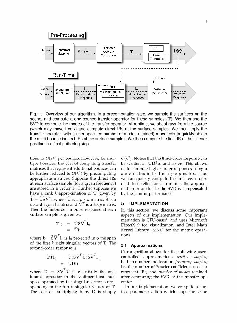
Fig. 1. Overview of our algorithm. In a precomputation step, we sample the surfaces on thescene, and compute a one-bounce transfer operator for these samples (T). We then use theSVD to compute the modes of the transfer operator. At runtime, we shoot rays from the source(which may move freely) and compute direct IRs at the surface samples. We then apply thetransfer operator (with a user-specified number of modes retained) repeatedly to quickly obtainthe multi-bounce indirect IRs at the surface samples. We then compute the final IR at the listenerposition in a final gathering step.

tions to O(pk) per bounce. However, for mul-tiple bounces, the cost of computing transfermatrices that represent additional bounces canbe further reduced to O(k2) by precomputingappropriate matrices. Suppose the direct IRsat each surface sample (for a given frequency)are stored in a vector l0. Further suppose wehave a rank k approximation of T, given byT = USV

T, where U is a p× k matrix, S is a

k×k diagonal matrix and VT is a k×p matrix.Then the first-order impulse response at eachsurface sample is given by:

Tl0 = USVTl0

= Ub

where b = SVTl0 is l0 projected into the span

of the first k right singular vectors of T. Thesecond-order response is:

TTl0 = U(SVTU)SV

Tl0

= UDb

where D = SVTU is essentially the one-

bounce operator in the k-dimensional sub-space spanned by the singular vectors corre-sponding to the top k singular values of T.The cost of multiplying b by D is simply

O(k2). Notice that the third-order response canbe written as UD2b, and so on. This allowsus to compute higher-order responses using ak × k matrix instead of a p × p matrix. Thuswe can quickly compute the first few ordersof diffuse reflection at runtime; the approxi-mation error due to the SVD is compensatedby the gain in performance.

5 IMPLEMENTATION

In this section, we discuss some importantaspects of our implementation. Our imple-mentation is CPU-based, and uses MicrosoftDirectX 9 for visualization, and Intel MathKernel Library (MKL) for the matrix opera-tions.

5.1 ApproximationsOur algorithm allows for the following user-controlled approximations: surface samples,both in number and location; frequency samples,i.e. the number of Fourier coefficients used torepresent IRs; and number of modes retainedafter computing the SVD of the transfer op-erator.

In our implementation, we compute a sur-face parameterization which maps the scene

7

primitives to the unit square (essentially auv texture mapping). This parameterizationis computed using Least Squares ConformalMapping (LSCM) [33]. We allow the user tospecify the texture dimensions; each texel ofthe resulting texture is mapped to a single sur-face sample using an inverse mapping process.The number of texels mapped to a given prim-itive is weighted by the area of the primitive,to ensure a roughly even distribution of sam-ples. We chose the LSCM algorithm for thispurpose since our modeling tools (Blender 1)have an implementation built-in; it can be re-placed with any other technique for samplingthe surfaces as long as the number of samplesgenerated on a primitive is proportional to itsarea.

Our implementation allows the user to varythe number of Fourier coefficients used torepresent the IRs. It has been shown [19]that 1K Fourier coefficients can provide anacceptable compromise between performanceand quality, and therefore we use 1K Fouriercoefficients for all our experiments.

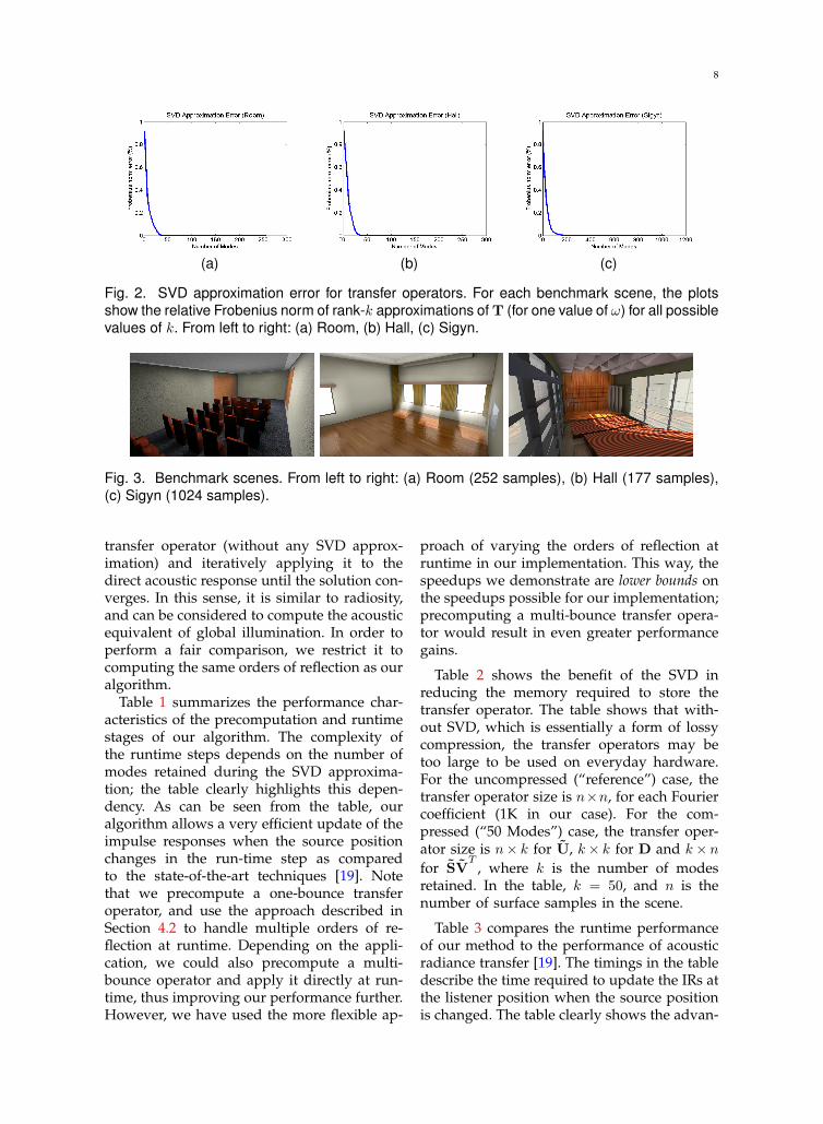
We measure the error caused by the SVD ap-proximation of the transfer operator in termsof the Frobenius norm. Figure 2 plots theFrobenius norm error against the number ofmodes retained for the transfer operator (T).The figure clearly shows that we could use avery small number of modes to compute IRswith diffuse reflections at runtime.

5.2 Audio Processing

As described in Section 3 the pressure signalat a source is convolved with an IR from thesource to a listener to compute the final audioat the listener. The algorithm presented in Sec-tion 4 computes a frequency domain energyIR with 1K Fourier coefficients. The pressureIR is computed from the energy IR [34] andupsampled to encode the desired propagationdelay in the IR [19].

Moving sources and listeners: In typicalvirtual environments applications, the sourceand listener are moving and the audio isstreaming from a source in chunks of audiosamples (called audio frames). The size of theaudio frames is determined by the allowedlatency for the application. We choose audio

1. http://www.blender.org

frames of 4800 samples at sampling rate of48KHz leading to a 100ms latency in our audiooutput. For a static source and listener, com-puting the final audio is trivial and amountsto convolving each audio frame with the IRto compute output audio frames. For movingsources and listeners, IRs evolve over timewhich could lead to discontinuities in the fi-nal audio when using different IRs for twoadjacent audio frames. In order to minimizesuch discontinuity artifacts, windowing [35] isapplied at the source frame and the listenerframe when the source and listener are mov-ing respectively. The windowing applied byour audio processing step is similar to Siltanenet. al. [19].

6 RESULTS

In this section, we present some experimen-tal results on the performance and qualityachieved by our implementation of our al-gorithm. All of our tests were performed onan Intel Xeon X5560 workstation with 4 cores(each operating at 2.80 GHz) and 4GB of RAMrunning Windows Vista. MKL parallelizes ourmatrix operations over all 4 cores of the testmachine. Therefore, the timings we report arefor all 4 cores. We have benchmarked ourimplementation on three scenes whose com-plexity is typical of scenes encountered inacoustics applications. Figure 3 shows thesescenes along with some details.

For comparison, we chose the state-of-the-art frequency acoustic radiance transfer algo-rithm [19]. To the best of our knowledge, theonly other algorithms for simulating diffusereflections of sound are naıve time-domainradiance transfer and path tracing. Naıvetime-domain radiance transfer would requirea large amount of memory, and since thefrequency-domain radiance transfer approach[19] is superior to it in this regard, we chosenot to compare against the time-domain ra-diance transfer approach. Path tracing can beused for dynamic scenes, however, since thescene would have to be traversed millions oftimes per frame, we choose not to compare ouralgorithm with path tracing, since we restrictourselves to static scenes.

The frequency-domain acoustic radiancetransfer method [19] works by computing the

8

(a) (b) (c)

Fig. 2. SVD approximation error for transfer operators. For each benchmark scene, the plotsshow the relative Frobenius norm of rank-k approximations of T (for one value of ω) for all possiblevalues of k. From left to right: (a) Room, (b) Hall, (c) Sigyn.

Fig. 3. Benchmark scenes. From left to right: (a) Room (252 samples), (b) Hall (177 samples),(c) Sigyn (1024 samples).

transfer operator (without any SVD approx-imation) and iteratively applying it to thedirect acoustic response until the solution con-verges. In this sense, it is similar to radiosity,and can be considered to compute the acousticequivalent of global illumination. In order toperform a fair comparison, we restrict it tocomputing the same orders of reflection as ouralgorithm.

Table 1 summarizes the performance char-acteristics of the precomputation and runtimestages of our algorithm. The complexity ofthe runtime steps depends on the number ofmodes retained during the SVD approxima-tion; the table clearly highlights this depen-dency. As can be seen from the table, ouralgorithm allows a very efficient update of theimpulse responses when the source positionchanges in the run-time step as comparedto the state-of-the-art techniques [19]. Notethat we precompute a one-bounce transferoperator, and use the approach described inSection 4.2 to handle multiple orders of re-flection at runtime. Depending on the appli-cation, we could also precompute a multi-bounce operator and apply it directly at run-time, thus improving our performance further.However, we have used the more flexible ap-

proach of varying the orders of reflection atruntime in our implementation. This way, thespeedups we demonstrate are lower bounds onthe speedups possible for our implementation;precomputing a multi-bounce transfer opera-tor would result in even greater performancegains.

Table 2 shows the benefit of the SVD inreducing the memory required to store thetransfer operator. The table shows that with-out SVD, which is essentially a form of lossycompression, the transfer operators may betoo large to be used on everyday hardware.For the uncompressed (“reference”) case, thetransfer operator size is n×n, for each Fouriercoefficient (1K in our case). For the com-pressed (“50 Modes”) case, the transfer oper-ator size is n× k for U, k× k for D and k× nfor SV

T, where k is the number of modes

retained. In the table, k = 50, and n is thenumber of surface samples in the scene.

Table 3 compares the runtime performanceof our method to the performance of acousticradiance transfer [19]. The timings in the tabledescribe the time required to update the IRs atthe listener position when the source positionis changed. The table clearly shows the advan-

9

Scene Precomputation Time Modes RuntimeT SVD Initial Scatter Transfer Operator Final Gather

10 43.2 ms 24.0 ms 33.7 msRoom 14.2 s 94.5 s 25 45.8 ms 43.8 ms 35.0 ms

50 42.4 ms 84.3 ms 36.4 ms

10 37.8 ms 26.8 ms 31.5 msHall 13.1 s 93.1 s 25 37.1 ms 45.5 ms 30.2 ms

50 36.6 ms 79.7 ms 31.2 ms

Sigyn 6.31 min 50.9 min 50 164.1 ms 218.1 ms 109.9 ms

TABLE 1Performance characteristics of our algorithm. For each scene, we present the precomputation

time required by our algorithm for 1K Fourier coefficients. Under precomputation time, we showthe time required to compute the transfer operator, T, and the time required to compute its SVD

approximation. We also compare running times for varying numbers of modes from the SVD.The table shows the time spent at runtime in initial shooting from the source, applying the

transfer operator, and gathering the final IR at the listener position.

Scene Samples Reference 50 Modes

Room 177 250.6 161.6Hall 252 508.0 221.6Sigyn 1024 8388.6 839.2

TABLE 2Memory requirements of the transfer operators

computed by our algorithm with (column 4)and without (column 3) SVD compression.

Note that since the entries of each matrix arecomplex numbers, each entry requires 8 bytes

of storage. All sizes in the table are in MB.

tage of our approach. Since our precomputedtransfer operator is decoupled from the sourceposition, moving the source does not requireus to recompute the transfer operator; this factallows us to update the source position muchfaster than a straightforward acoustic radiancetransfer technique.

Figure 4 shows some impulse responsescomputed by our algorithm, as compared withthe reference acoustic radiance transfer case.As the figure shows, reducing the numberof modes has very little effect on the overallshape of the IRs. Coupled with the memorysavings demonstrated in Table 2 and perfor-mance advantage demonstrated in Table 3,we see that using the SVD allows us to sig-nificantly reduce memory requirements andincrease performance without significant ad-verse effects on the IRs computed. Of course,the best way to demonstrate the benefit of

our approach is by comparing audio clips; forthis we refer the reader to the accompanyingvideo.

7 CONCLUSIONWe have described a precomputed direct-to-indirect transfer approach to solving theacoustic rendering equation in the frequencydomain for diffuse reflections. We havedemonstrated that our approach is able toefficiently simulate early diffuse reflections fora moving source and listener in static scenes.In comparison with existing methods, our ap-proach offers a significant performance advan-tage when handling moving sources.

7.1 LimitationsOur approach has some limitations. Since itis a precomputed acoustic radiance transferalgorithm, it cannot be used for scenes withdynamic objects. In such situations, algorithmsbased on path tracing are the best avail-able choice. However, in many applications,including games and virtual environments,scenes are entirely or mostly static, with rel-atively few moving parts, and hence our al-gorithm can still be used to model reflectionswithin the static portions of the scene.

Our algorithm performs matrix-vector mul-tiplications on large matrices at runtime. Thesize of the matrix still depends on the surfacesize and complexity of the scene. Therefore,our method is useful mainly for scenes of lowto medium complexity.

10

Scene Orders Radiance Transfer Direct-to-Indirect Transfer(50 modes)

2 11.7 s 131.8 msRoom 5 11.8 s 154.4 ms

10 12.0 s 179.3 ms

2 10.6 s 116.5 msHall 5 10.7 s 147.3 ms

10 10.9 s 170.5 ms

2 185.3 s 468.5 msSigyn 5 186.7 s 491.2 ms

10 188.7 s 512.8 ms

TABLE 3Comparison of our approach with a straightfoward Acoustic Radiance Transfer approach [19].

We compare the time required by our algorithm to update the source position and recompute theIR at the listener position after a varying number of diffuse reflections. Since the Acoustic

Radiance Transfer approach does not decouple the transfer operator from the source position, itneeds to perform a costly recomputation of the transfer operator each time the source moves.

On the other hand, our algorithm quickly updates the direct IR at all surface samples, thenapplies the precomputed transfer operator. This allows our approach to handle moving sources

far more efficiently than the state-of-the-art.

(a) Room, reference (b) Room, 50 modes

(c) Hall, reference (d) Hall, 50 modes

Fig. 4. Comparison of second order diffuse IRs computed by our system with and without SVDcompression, for some of our benchmark scenes.

11

7.2 Future Work

Our algorithm uses 1K Fourier coefficients perIR, and this significantly increases our mem-ory requirements. It is crucial to develop anapproach to reduce these storage requirementsin order to make it feasible to implementon hardware such as video game consoles.It might be possible to use a representationbased on Raghuvanshi et al’s precomputednumerical simulation algorithm [11].

In most complex scenes, each surface sam-ple may influence only a subset of all sam-ples in the scene, due to occlusion effects.This observation motivates us to subdividethe scene into cells separated by portals. Wecould compute transfer operators for each cellindependently, and model the interchange ofsound energy at the portal boundaries. Cellsand portals have been previously used tomodel late reverberation [36], and would bea promising research direction for diffuse re-flections.

The acoustic response over the surfacesof the scene typically are smooth functions.Therefore, it would be beneficial to exploitthe spatial coherence of IRs by projecting thetransfer operator into basis functions definedover the surfaces of the scene. Furthermore,it might be interesting to investigate the pos-sibility of applying direct-to-indirect transfertechniques to the problem of non-diffuse re-flections or edge diffractions.

REFERENCES

[1] B.-I. Dalenback, M. Kleiner, and P. Svensson, “Amacroscopic view of diffuse reflection,” J. Audio Eng.Soc., vol. 42, pp. 793–807, 1994.

[2] B.-I. Dalenback, “The Importance of Diffuse Reflec-tion in Computerized Room Acoustic Prediction andAuralization,” in Proceedings of the Institute of Acous-tics (IOA), vol. 17, no. 1, 1995, pp. 27–33.

[3] R. R. Torres, M. Kleiner, and B.-I. Dalenback,“Audibility of ”diffusion” in room acoustics au-ralization: An initial investigation,” Acta Acusticaunited with Acustica, vol. 86, pp. 919–927(9), Novem-ber/December 2000.

[4] P.-P. Sloan, J. Kautz, and J. Snyder, “Precomputedradiance transfer for real-time rendering in dy-namic, low-frequency lighting environments,” inSIGGRAPH ’02: Proceedings of the 29th annual confer-ence on Computer graphics and interactive techniques.New York, NY, USA: ACM, 2002, pp. 527–536.

[5] M. Hasan, F. Pellacini, and K. Bala, “Direct-to-indirect transfer for cinematic relighting,” in SIG-GRAPH ’06: ACM SIGGRAPH 2006 Papers. NewYork, NY, USA: ACM, 2006, pp. 1089–1097.

[6] J. Lehtinen, M. Zwicker, E. Turquin, J. Kontkanen,F. Durand, F. X. Sillion, and T. Aila, “A meshlesshierarchical representation for light transport,” inSIGGRAPH ’08: ACM SIGGRAPH 2008 papers. NewYork, NY, USA: ACM, 2008, pp. 1–9.

[7] P. Svensson and R. Kristiansen, “Computationalmodelling and simulation of acoustic spaces,” in22nd International Conference: Virtual, Synthetic, andEntertainment Audio, June 2002.

[8] R. Ciskowski and C. Brebbia, Boundary Element meth-ods in acoustics. Computational Mechanics Publica-tions and Elsevier Applied Science, 1991.

[9] N. Raghuvanshi, N. Galoppo, and M. C. Lin, “Ac-celerated wave-based acoustics simulation,” in SPM’08: Proceedings of the 2008 ACM symposium on Solidand physical modeling. New York, NY, USA: ACM,2008, pp. 91–102.

[10] F. Ihlenburg, Finite Element Analysis of Acoustic Scat-tering. Springer Verlag AG, 1998.

[11] N. Raghuvanshi, J. Snyder, R. Mehra, M. Lin, andN. Govindaraju, “Precomputed wave simulation forreal-time sound propagation of dynamic sources incomplex scenes,” in Proc. SIGGRAPH 2010 (To ap-pear), 2010.

[12] M. Vorlander, “Simulation of the transient andsteady-state sound propagation in rooms using anew combined ray-tracing/image-source algorithm,”The Journal of the Acoustical Society of America,vol. 86, no. 1, pp. 172–178, 1989. [Online]. Available:http://link.aip.org/link/?JAS/86/172/1

[13] B. Kapralos, M. Jenkin, and E. Milios, “Sonel map-ping: acoustic modeling utilizing an acoustic versionof photon mapping,” in In IEEE International Work-shop on Haptics Audio Visual Environments and theirApplications (HAVE 2004), 2004, pp. 2–3.

[14] A. Chandak, C. Lauterbach, M. Taylor, Z. Ren, andD. Manocha, “Ad-frustum: Adaptive frustum tracingfor interactive sound propagation,” IEEE Transactionson Visualization and Computer Graphics, vol. 14, no. 6,pp. 1707–1722, 2008.

[15] M. T. Taylor, A. Chandak, L. Antani, andD. Manocha, “Resound: interactive sound renderingfor dynamic virtual environments,” in MM ’09:Proceedings of the seventeen ACM internationalconference on Multimedia. New York, NY, USA:ACM, 2009, pp. 271–280.

[16] T. Funkhouser, I. Carlbom, G. Elko, G. Pingali,M. Sondhi, and J. West, “A beam tracing approachto acoustic modeling for interactive virtual environ-ments,” in Proc. of ACM SIGGRAPH, 1998, pp. 21–32.

[17] A. Chandak, L. Antani, M. Taylor, andD. Manocha, “Fastv: From-point visibilityculling on complex models,” Computer GraphicsForum, vol. 28, pp. 1237–1246(10), 2009. [On-line]. Available: http://www.ingentaconnect.com/content/bpl/cgf/2009/00000028/00000004/art00020

[18] S. Siltanen, T. Lokki, S. Kiminki, and L. Savioja, “Theroom acoustic rendering equation.” The Journal of theAcoustical Society of America, vol. 122, no. 3, pp. 1624–1635, September 2007.

[19] S. Siltanen, T. Lokki, and L. Savioja, “Frequencydomain acoustic radiance transfer for real-timeauralization,” Acta Acustica united with Acustica,vol. 95, pp. 106–117(12), 2009. [Online]. Avail-able: http://www.ingentaconnect.com/content/dav/aaua/2009/00000095/00000001/art00010

[20] U. P. Svensson, R. I. Fred, and J. Vanderkooy, “Ananalytic secondary source model of edge diffraction

12

impulse responses ,” Acoustical Society of AmericaJournal, vol. 106, pp. 2331–2344, Nov. 1999.

[21] M. Taylor, A. Chandak, Z. Ren, C. Lauterbach, andD. Manocha, “Fast edge-diffraction for sound prop-agation in complex virtual environments,” in EAAAuralization Symposium, 2009.

[22] D. Schroder and A. Pohl, “Real-time hybrid simu-lation method including edge diffraction,” in EAAAuralization Symposium, 2009.

[23] C. M. Goral, K. E. Torrance, D. P. Greenberg, andB. Battaile, “Modeling the interaction of light be-tween diffuse surfaces,” SIGGRAPH Comput. Graph.,vol. 18, no. 3, pp. 213–222, 1984.

[24] Y.-T. Tsai and Z.-C. Shih, “All-frequency precom-puted radiance transfer using spherical radial basisfunctions and clustered tensor approximation,” ACMTrans. Graph., vol. 25, no. 3, pp. 967–976, 2006.

[25] A. W. Kristensen, T. Akenine-Moller, and H. W.Jensen, “Precomputed local radiance transfer forreal-time lighting design,” in SIGGRAPH ’05: ACMSIGGRAPH 2005 Papers. New York, NY, USA: ACM,2005, pp. 1208–1215.

[26] J. Kontkanen, E. Turquin, N. Holzschuch,and F. Sillion, “Wavelet radiance transportfor interactive indirect lighting,” in RenderingTechniques 2006 (Eurographics Symposium onRendering), W. Heidrich and T. Akenine-Moller,Eds. Eurographics, jun 2006. [Online]. Available:http://artis.imag.fr/Publications/2006/KTHS06

[27] R. Wang, J. Zhu, and G. Humphreys, “Precomputedradiance transfer for real-time indirect lighting usinga spectral mesh basis,” in Proceedings of the Eurograph-ics Symposium on Rendering, 2007.

[28] T. Funkhouser, N. Tsingos, and J.-M. Jot, “Survey ofmethods for modeling sound propagation in interac-tive virtual environment systems,” Presence, 2003.

[29] H. Kuttruff, Room Acoustics. Elsevier Science Pub-lishing Ltd., 1991.

[30] J. T. Kajiya, “The rendering equation,” in SIGGRAPH’86: Proceedings of the 13th annual conference on Com-puter graphics and interactive techniques. New York,NY, USA: ACM, 1986, pp. 143–150.

[31] R. N. Bracewell, The Fourier transform and its applica-tions. McGraw-Hill, 2000.

[32] E. O. Brigham, The Fast Fourier Transform and itsapplications. Prentice-Hall, 1988.

[33] B. Levy, S. Petitjean, N. Ray, and J. Maillot, “Leastsquares conformal maps for automatic texture atlasgeneration,” ACM Trans. Graph., vol. 21, no. 3, pp.362–371, 2002.

[34] H. K. Kuttruff, “Auralization of Impulse ResponsesModeled on the Basis of Ray-Tracing Results,” Jour-nal of the Audio Engineering Society, vol. 41, no. 11,pp. 876–880, November 1993.

[35] A. V. Oppenheim, R. W. Schafer, and J. R. Buck,Discrete-Time Signal Processing, 2nd ed. Prentice Hall,January 1999.

[36] E. Stavrakis, N. Tsingos, and P. Calamia, “Topologicalsound propagation with reverberation graphs,” ActaAcustica/Acustica - the Journal of the European AcousticsAssociation (EAA), 2008. [Online]. Available: http://www-sop.inria.fr/reves/Basilic/2008/STC08