NBER WORKING PAPER SERIES

DISCRETION IN HIRING

Mitchell HoffmanLisa B. KahnDanielle Li

Working Paper 21709http://www.nber.org/papers/w21709

NATIONAL BUREAU OF ECONOMIC RESEARCH1050 Massachusetts Avenue

Cambridge, MA 02138November 2015

We are grateful to Jason Abaluck, Ricardo Alonso, David Berger, Arthur Campbell, David Deming,Alex Frankel, Harry Krashinsky, Jin Li, Liz Lyons, Steve Malliaris, Mike Powell, Kathryn Shaw, SteveTadelis, and numerous seminar participants. We are grateful to the anonymous data provider for providingaccess to proprietary data. Hoffman acknowledges financial support from the Social Science and HumanitiesResearch Council of Canada. All errors are our own. The views expressed herein are those of the authorsand do not necessarily reflect the views of the National Bureau of Economic Research.

NBER working papers are circulated for discussion and comment purposes. They have not been peer-reviewed or been subject to the review by the NBER Board of Directors that accompanies officialNBER publications.

© 2015 by Mitchell Hoffman, Lisa B. Kahn, and Danielle Li. All rights reserved. Short sections oftext, not to exceed two paragraphs, may be quoted without explicit permission provided that full credit,including © notice, is given to the source.

Discretion in HiringMitchell Hoffman, Lisa B. Kahn, and Danielle LiNBER Working Paper No. 21709November 2015JEL No. J24,M51

ABSTRACT

Who should make hiring decisions? We propose an empirical test for assessing whether firms shouldrely on hard metrics such as job test scores or grant managers discretion in making hiring decisions.We implement our test in the context of the introduction of a valuable job test across 15 firms employinglow-skill service sector workers. Our results suggest that firms can improve worker quality by limitingmanagerial discretion. This is because, when faced with similar applicant pools, managers who exercisemore discretion (as measured by their likelihood of overruling job test recommendations) systematicallyend up with worse hires.

Mitchell HoffmanUniversity of TorontoRotman School of Management105 St. George St.Toronto, ON M5S-3E6Canadamitchell.hoffman@rotman.utoronto.ca

Lisa B. KahnYale UniversitySchool of ManagementP. O. Box 208200New Haven, CT 06520and NBERlisa.kahn@yale.edu

Danielle LiHarvard Business School211 Rock CenterBoston, MA 02163dli@hbs.edu

1 Introduction

Hiring the right workers is one of the most important and di�cult problems that a �rm

faces. Resumes, interviews, and other screening tools are often limited in their ability to

reveal whether a worker has the right skills or will be a good �t. Further, the managers

that �rms employ to gather and interpret this information may have poor judgement or

preferences that are imperfectly aligned with �rm objectives.1 Firms may thus face both

information and agency problems when making hiring decisions.

The increasing adoption of �workforce analytics� and job testing has provided �rms

with new hiring tools.2 Job testing has the potential to both improve information about the

quality of candidates and to reduce agency problems between �rms and human resource (HR)

managers. As with interviews, job tests provide an additional signal of a worker's quality.

Yet, unlike interviews and other subjective assessments, job testing provides information

about worker quality that is directly veri�able by the �rm.

What is the impact of job testing on the quality of hires and how should �rms use job

tests, if at all? In the absence of agency problems, �rms should allow managers discretion to

weigh job tests alongside interviews and other private signals when deciding whom to hire.

Yet, if managers are biased or if their judgment is otherwise �awed, �rms may prefer to

limit discretion and place more weight on test results, even if this means ignoring the private

information of the manager. Firms may have di�culty evaluating this trade o� because they

cannot tell whether a manager hires a candidate with poor test scores because he or she has

private evidence to the contrary, or because he or she is biased or simply mistaken.

In this paper, we evaluate the introduction of a job test and develop a diagnostic to

inform how �rms should incorporate it into their hiring decisions. Using a unique personnel

dataset on HR managers, job applicants, and hired workers across 15 �rms that adopt job

testing, we present two key �ndings. First, job testing substantially improves the match

quality of hired workers: those hired with job testing have about 15% longer tenures than

1For example, a manager could have preferences over demographics or family background that do notmaximize productivity. In a case study of elite professional services �rms, Riviera (2012) shows that one ofthe most important determinants of hiring is the presence of shared leisure activities.

2See, for instance, Forbes: http://www.forbes.com/sites/joshbersin/2013/02/17/bigdata-in-human-resources-talent-analytics-comes-of-age/.

1

those hired without testing. Second, managers who overrule test recommendations more

often hire workers with lower match quality, as measured by job tenure. This second result

suggests that managers exercise discretion because they are biased or have poor judgement,

not because they are better informed. This implies that �rms in our setting can further

improve match quality by limiting managerial discretion and placing more weight on the

test.

Our paper makes the following contributions. First, we provide new evidence that

managers systematically make hiring decisions that are not in the interest of the �rm. This

generates increased turnover in a setting where workers already spend a substantial fraction

of their tenure in paid training. Second, we show that job testing can improve hiring outcomes

not simply by providing more information, but by making information veri�able, and thereby

expanding the scope for contractual solutions to agency problems within the �rm. Finally,

we develop a simple tractable test for assessing the value of discretion in hiring. Our test

uses data likely available to any �rm with job testing, and is applicable to a wide variety of

settings where at least one objective correlate of productivity is available.

We begin with a model in which �rms rely on potentially biased HR managers who

observe both public and private signals of worker quality. Using this model, we develop a

simple empirical diagnostic based on the following intuition: if managers make exceptions

to test recommendations because they have superior private information about a worker's

quality, then we would expect better informed managers to both be more likely to make

exceptions and to hire workers who are a better �t. As such, a positive correlation between

exceptions and outcomes suggests that the discretion granted was valuable. If, in contrast,

managers who make more exceptions hire workers with worse outcomes, then it is likely that

managers are either biased or mistaken, and �rms should limit discretion.

We apply this test using data from an anonymous �rm that provides online job testing

services to client �rms. Our sample consists of 15 client �rms who employ low-skill service-

sector workers. Prior to the introduction of testing, �rms employed HR managers involved in

hiring new workers. After the introduction of testing, HR managers were also given access to

a test score for each applicant: green (high potential candidate), yellow (moderate potential

2

candidate), or red (lowest rating).3 Managers were encouraged to factor the test into their

hiring decisions but were still given discretion to use other signals of quality.

First, we estimate the impact of introducing a job test on the match quality of hired

workers. By examining the staggered introduction of job testing across our sample locations,

we show that cohorts of workers hired with job testing have about 15% longer tenures than

cohorts of workers hired without testing. We provide a number of tests in the paper to ensure

that our results are not driven by the endogenous adoption of testing or by other policies

that �rms may have concurrently implemented.

This �nding suggests that job tests contain valuable information about the match qual-

ity of candidates. Next, we ask how �rms should use this information, in particular, whether

�rms should limit discretion and follow test recommendations, or allow managers to exercise

discretion and make exceptions to those recommendations. A unique feature of our data is

that it allows us to measure the exercise of discretion explicitly: we observe when a manager

hires a worker with a test score of yellow when an applicant with a score of green goes unhired

(or similarly, when a red is hired above a yellow or a green). As explained above, the corre-

lation between a manager's likelihood of making these exceptions and eventual outcomes of

hires can inform whether the exercise of discretion is bene�cial from the �rm's perspective.

Across a variety of speci�cations, we �nd that the exercise of discretion is strongly correlated

with worse outcomes. Even when faced with applicant pools that are identical in terms of

test scores, managers that make more exceptions systematically hire workers who are more

likely to quit or be �red.

Finally, we show that our results are unlikely to be driven by the possibility that man-

agers sacri�ce job tenure in search of workers who have higher quality on other dimensions.

If this were the case, limiting discretion may improve worker durations, but at the expense of

other quality measures. To assess whether this is a possible explanation for our �ndings, we

examine the relationship between hiring, exceptions, and a direct measure of productivity,

daily output per hour, which we observe for a subset of �rms in our sample. Based on this

supplemental analysis, we no evidence that �rms are trading o� duration for higher produc-

3Section 2 provides more information on the job test.

3

tivity. Taken together, our �ndings suggest that �rms could improve both match quality

and worker productivity by placing more weight on the recommendations of the job test.

As data analytics becomes more frequently applied to human resource management de-

cisions, it becomes increasingly important to understand how these new technologies impact

the organizational structure of the �rm and the e�ciency of worker-�rm matching. While

a large theoretical literature has studied how �rms should allocate authority, ours is the

�rst paper to provide an empirical test for assessing the value of discretion in hiring.4 Our

�ndings provide direct evidence that screening technologies can help resolve agency problems

by improving information symmetry, and thereby relaxing contracting constraints. In this

spirit, our paper is related to the classic Baker and Hubbard (2004) analysis of the adoption

of on board computers in the trucking industry.

We also contribute to a small, but growing literature on the impact of screening tech-

nologies on the quality of hires.5 Our work is most closely related to Autor and Scarborough

(2008), the �rst paper in economics to provide an estimate of the impact of job testing on

worker performance. The authors evaluate the introduction of a job test in retail trade,

with a particular focus on whether testing will have a disparate impact on minority hiring.

Our paper, by contrast, studies the implications of job testing on the allocation of authority

within the �rm.

Our work is also relevant to a broader literature on hiring and employer learning.6 Oyer

and Schaefer (2011) note in their handbook chapter that hiring remains an important open

4For theoretical work, see Bolton and Dewatripont (2012) for a survey and Dessein (2002) and Alonsoand Matouschek (2008) for particularly relevant instances. There is a small empirical literature on bias,discretion and rule-making in other settings. For example, Paravisini and Schoar (2012) �nd that creditscoring technology aligns loan o�er incentives and improves lending performance. Li (2012) documents anempirical tradeo� between expertise and bias among grant selection committees. Kuziemko (2013) showsthat the exercise of discretion in parole boards is e�cient, relative to �xed sentences.

5Other screening technologies include labor market intermediaries (e.g., Autor (2001), Stanton andThomas (2014), Horton (2013)), and employee referrals (e.g., Brown et al., (2015), Burks et al. (2015)and Pallais and Sands (2015)).

6A central literature in labor economics emphasizes that imperfect information generates substantialproblems for allocative e�ciency in the labor market. This literature suggests imperfect information is asubstantial problem facing those making hiring decisions. See for example Jovanovic (1979), Farber andGibbons (1996), Altonji and Pierret (2001), and Kahn and Lange (2014).

4

area of research. We point out that hiring is made even more challenging because �rms must

often entrust these decisions to managers who may be biased or exhibit poor judgment.7

Lastly, our results are broadly aligned with �ndings in psychology and behavioral eco-

nomics that emphasize the potential of machine-based algorithms to mitigate errors and

biases in human judgement across a variety of domains.8

The remainder of this paper proceeds as follows. Section 2 describes the setting and

data. Section 3 evaluates the impact of testing on the quality of hires. Section 4 presents

a model of hiring with both hard and soft signals of quality. Section 5 evaluates the role of

discretion in test adoption. Section 6 concludes.

2 Setting and Data

Firms have increasingly incorporated testing into their hiring practices. One explanation

for this shift is that the increasing power of data analytics has made it easier to look for

regularities that predict worker performance. We obtain data from an anonymous job testing

provider that follows such a model. We hereafter term this �rm the �data �rm.� In this

section we summarize the key features of our dataset. More detail can be found in Appendix

A.

The data �rm o�ers a test designed to predict performance for a particular job in the

low-skilled service sector. To preserve the con�dentiality of the data �rm, we are unable

to reveal the exact nature of the job, but it is similar to jobs such as data entry work,

standardized test grading, and call center work (and is not a retail store job). The data �rm

sells its services to clients (hereafter, �client �rms�) that wish to �ll these types of positions.

We have 15 such client �rms in our dataset.

The job test consists of an online questionnaire comprising a large battery of questions,

including those on technical skills, personality, cognitive skills, �t for the job, and various job

scenarios. The data �rm matches applicant responses with subsequent performance in order

7This notion stems from the canonical principal-agent problem, for instance as in Aghion and Tirole(1997). In addition, many other models of management focus on moral hazard problems generated when amanager is allocated decision rights.

8See Kuncel et. al. (2013) for a meta-analysis of this literature and Kahneman (2011) for a behavioraleconomics perspective.

5

to identify the various questions that are the most predictive of future workplace success in

this setting. Drawing on these correlations, a proprietary algorithm delivers a green, yellow,

red job test score.

In its marketing materials, our data �rm emphasizes the ability of its job test to reduce

worker turnover, which is a perennial challenge for �rms employing low skill service sector

workers. To illustrate this concern, Figure 1 shows a histogram of job tenure for completed

spells (75% of the spells in our data) among employees in our sample client �rms. The

median worker (solid red line) stays only 99 days, or just over 3 months. Twenty percent of

hired workers leave after only a month. At the same time, our client �rms generally report

spending the �rst several weeks training each new hire, during which time the hire is being

paid.9 Correspondingly, our analysis will also focus on job retention as the primary measure

of hiring quality. For a subset of our client �rms we also observe a direct measure of worker

productivity: output per hour.10 Because these data are available for a much smaller set of

workers (roughly a quarter of hired workers), we report these �ndings separately when we

discuss alternative explanations.

Prior to testing, our client �rms gave their managers discretion to make hiring decisions

or recommendations based on interviews and resumes.11 After testing, �rms made scores

available to managers and encouraged them to factor scores into hiring recommendations,

but authority over hiring decisions was still typically delegated to managers.12

Our data contain information on hired workers, including hire and termination dates,

the reason for the exit, job function, and worker location. This information is collected by

client �rms and shared with the data �rm. In addition, once a partnership with the data

�rm forms, we can also observe applicant test scores, application date, and an identi�er for

the HR manager responsible for a given applicant.

9Each client �rm in our sample provides paid training to its workforce. Reported lengths of training varyconsiderably, from around 1-2 weeks to around a couple months or more.

10A similar productivity measure was used in Lazear et al., (2015) to evaluate the value of bosses in acomparable setting to ours.

11In addition, the data �rm informed us that a number of client �rms had some other form of testingbefore the introduction of the data �rm's test.

12We do not directly observe authority relations in our data. However, drawing on information for severalclient �rms (information provided by the data �rm), managers were not required to hire strictly by the test.

6

In the �rst part of this paper, we examine the impact of testing technology on worker

match quality, as measured by tenure. For any given client �rm, testing was rolled out grad-

ually at roughly the location level. During the period in which the test is being introduced,

not all applicants to the same location received test scores.13 We therefore impute a location-

speci�c date of testing adoption. Our preferred metric for the date of testing adoption is the

�rst date in which at least 50% of the workers hired in that month and location have a test

score. Once testing is adopted at a location, based on our de�nition, we impose that testing

is thereafter always available.14 In practice, this choice makes little di�erence and we are

robust to a number of other de�nitions, for example, whether the individual or any hire in

a cohort has a job test score.

Table 1 provides sample characteristics. Across our whole sample period we have nearly

300,000 hires; two-thirds of these were observed before testing was introduced and one-third

were observed after, based on our preferred imputed de�nition of testing. Once we link

applicants to the HR manager responsible for them (only after testing), we have 555 such

managers in the data.15 These managers primarily serve a recruiting role, and are unlikely

to manage day-to-day production. Post-testing, when we have information on applicants as

well as hires, we have nearly 94,000 hires and a total of 690,000 applicants.

Table 1 also reports worker performance pre- and post-testing, by test score. On av-

erage, greens stay 12 days (11%) longer than yellows, who stay 17 days (18%) longer than

reds. These di�erences are statistically signi�cant and hold up to the full range of controls

described below. This provides some evidence that test scores are indeed informative about

worker performance. Even among the selected sample of hired workers, better test scores

predict longer tenures. We might expect these di�erences to be even larger in the overall ap-

plicant population if managers hire red and yellow applicants only when unobserved quality

is particularly high. On our productivity measure, output per hour, which averages roughly

8, performance is fairly similar across color.

13We are told by the data �rm, however, that the intention of clients was generally to bring testing into alocation at the same time for workers in that location.

14This �ts patterns in the data, for example, that most locations weakly increase the share of applicantsthat are tested throughout our sample period.

15The HR managers we study are referred to as recruiters by our data provider. Other managers may takepart in hiring decisions as well. One �rm said that its recruiters will often endorse candidates to anothermanager (e.g., a manager in operations one rank above the frontline supervisor) who will make a ��nal call.�

7

3 The Impact of Testing

3.1 Empirical Strategy

Before examining whether �rms should grant managers discretion over how to use job

testing information, we �rst evaluate the impact of introducing testing information itself. To

do so, we exploit the gradual roll-out in testing across locations and over time, and examine

its impact on worker match quality, as measured by tenure:

Outcomelt = α0 + α1Testinglt + δl + γt + Controls + εlt (1)

Equation (1) compares outcomes for workers hired with and without job testing. We

regress a productivity outcome (Outcomelt) for workers hired to a location l, at time t,

on an indicator for whether testing was available at that location at that time (Testinglt)

and controls. In practice, we de�ne testing availability as whether the median hire at that

location-date was tested, though we discuss robustness to other measures. As mentioned

above, the location-time-speci�c measure of testing availability is preferred to using an indi-

cator for whether an individual was tested (though we also report results with this metric)

because of concerns that an applicant's testing status is correlated with his or her perceived

quality. We estimate these regressions at the location-time (month-by-year) level, the level

of variation underlying our key explanatory variable, and weight by number of hires in a

location-date.16 The outcome measure is the average outcome for workers hired to the same

location at the same time.

All regressions include a complete set of location (δl) and month by year of hire (γt)

�xed e�ects. They control for time-invariant di�erences across locations within our client

�rms, as well as for cohort and macroeconomic e�ects that may impact job duration. We also

experiment with a number of additional control variables, described in our results section,

below. In all speci�cations, standard errors are clustered at the location level to account for

correlated observations within a location over time.

16This aggregation a�ords substantial savings on computation time, and, will produce identical results tothose from a worker-level regression, given the regression weights.

8

Our primary outcome measure, Outcomelt, is the log of the length of completed job

spells, averaged across workers hired to �rm-location l, at time t. We focus on this, and

other outcomes related to the length of job spells, for several reasons. The length of a job

spell is a measure that both theory and the �rms in our study agree is important. Canonical

models of job search (e.g., Jovanovic 1979), predict a positive correlation between match

quality and job duration. Moreover, as discussed in Section 2, our client �rms employ low-

skill service sector workers and face high turnover and training costs: several weeks of paid

training in a setting where the median worker stays only 99 days (see Figure 1.) Job duration

is also a measure that has been used previously in the literature, for example by Autor and

Scarborough (2008), who also focus on a low-skill service sector setting (retail). Finally, job

duration is available for all workers in our sample.

3.2 Results

Table 2 reports regression results for the log duration of completed job spells. We

later report results for several duration-related outcomes that do not restrict the sample

to completed spells. Of the 270,086 hired workers that we observe in our sample, 75%, or

202,728 workers have completed spells (4,401 location-month cohorts), with an average spell

lasting 203 days and a median spell of 99 days. The key explanatory variable is whether or

not the median hire at this location-date was tested.

In the baseline speci�cation (Panel 1, Column 1 of Table 2) we �nd that employees

hired with the assistance of job testing stay, on average, 0.272 log points, or 31% longer,

signi�cant at the 5% level.

Panel 1 Column 2 introduces client �rm-by-year �xed e�ects to control for the imple-

mentation of any new strategies and HR policies that �rms may have adopted along with

testing.17 In this speci�cation, we compare locations in the same �rm in the same year, some

of which receive job testing sooner than others. The identifying assumption is that, within

a �rm, locations that receive testing sooner vs. later were on parallel trends before testing.

17Our data �rm has indicated that it was not aware of other client-speci�c policy changes, though theyacknowledge they would not have had full visibility into whether such changes may have occurred.

9

Here our estimated coe�cient falls by roughly a third in magnitude, and we lose statistical

signi�cance.

To account for the possibility that the timing of the introduction of testing is related

to trends at the location level, for example, that testing was introduced �rst to the locations

that were on an upward (or downward) trajectory, Column 3 introduces location-speci�c

time trends. These trends also account for broad trends that may impact worker retention,

for instance, smooth changes in local labor market conditions. Adding these controls reduces

the magnitude of our estimate but also greatly reduces the standard errors. We thus estimate

an increased completed job duration of 0.137 log points or 15%, signi�cant at the 5%-level.

Finally, in Column 4, we add controls for the composition of the applicant pool at a

location after testing is implemented: �xed e�ects for the number of green, yellow, and red

applicants. Because these variables are de�ned only after testing, these controls should be

thought of as interactions between composition and the post-testing indicator, and are set

to zero pre-testing. With these controls, the coe�cient α1 on Testinglt is the impact of the

introduction of testing, for locations that end up receiving similarly quali�ed applicants.

However, these variables also absorb any impact of testing on the quality of applicants that

a location receives. For instance, the introduction of testing may have a screening e�ect: as

candidates gradually learn about testing, the least quali�ed may be deterred from applying.

Our point estimate remains unchanged with the inclusion of this set of controls, but the

standard errors do increase substantially. This suggests that match quality improves because

testing aids managers in identifying productive workers, rather than by exclusively altering

the quality of the applicant pool. Overall, the range of estimates in Table 2 are similar to

previous estimates found in Autor and Scarborough (2008).

Panel 2 of Table 2 examines robustness to de�ning testing at the individual level. For

these speci�cations we regress an individual's job duration (conditional on completion) on

whether or not the individual was tested. Because these speci�cations are at the individual

level, our sample size increases from 4,401 location-months to 202,728 individual hiring

events. Using these same controls, we �nd numerically similar estimates. The one exception

is Column 4, which is now signi�cant and larger: a 26% increase. From now on, we continue

with our preferred metric of testing adoption (whether the median worker was tested).

10

Figure 2 shows event studies where we estimate the treatment impact of testing by

quarter, from 12 quarters before testing to 12 quarters after testing, using our baseline set

of controls. The top left panel shows the event study using log length of completed tenure

spells as the outcome measure. The �gure shows that locations that will obtain testing

within the next few months look very similar to those that will not (because they either

have already received testing or will receive it later). After testing is introduced, however,

we begin to see large di�erences. The treatment e�ect of testing appears to grow over time,

suggesting either that HR managers and other participants might take some time to learn

how to use the test e�ectively. This alleviates any concerns that any systematic di�erences

across locations drive the timing of testing adoption.

We also explore a range of other duration-related outcomes to examine whether the

impact of testing is concentrated at any point in the duration distribution. For each hired

worker, we measure whether they stay at least three, six, or twelve months, for the set of

workers who are not right-censored.18 We aggregate this variable to measure the proportion

of hires in a location-cohort that meet each duration milestone. Regression results (analogous

to those reported in Panel 1 of Table 2 are reported in Appendix Table A1, while event studies

are shown in the remaining panels of Figure 2. For each of these measures, we again see that

testing improves job durations, and we see no evidence of any pre-trends.

This section thus establishes that the adoption of testing improves outcomes of hired

workers. We next ask whether �rms should change their hiring practices given they now

have access to an apparently valuable signal of applicant quality.

4 Model

We formalize a model in which a �rm makes hiring decisions with the help of an HR

manager. There are two sources of information about the quality of job candidates. First,

interviews generate unveri�able information about a candidate's quality that is privately

observed by the HR manager. Second, the job testing provides veri�able information about

18That is, a worker will be included in this metric if his or her hire date was at least three, six, or twelvemonths, respectively, before the end of data collection.

11

quality that is observed by both the manager and the �rm. Managers then make hiring

recommendations with the aid of both sources of information.

In this setting, job testing can improve hiring in two ways. First, it can help managers

make more informed choices by providing an additional signal of worker quality. Second,

because test information is veri�able, it enables the �rm to constrain biased managers.

Granting managers discretion enables the �rm to take advantage of both interview and

test signals, but may also leave it vulnerable to managerial biases. Limiting discretion and

relying on the test removes scope for bias, but at the cost of ignoring private information.

The following model formalizes this tradeo� and outlines an empirical test of whether �rms

can improve worker quality by eliminating discretion.

4.1 Setup

A mass one of applicants apply for job openings within a �rm. The �rm's payo� of

hiring worker i is given by the worker's match quality, ai. We assume that ai is drawn from

a distribution which depends on a worker's type, ti ∈ {G, Y }; a share of workers pG are type

G, a share 1 − pG are type Y , and a|t ∼ N(µt, σ2a) with µG > µY and σ2

a ∈ (0,∞). This

match quality distribution enables us to naturally incorporate the discrete test score into

the hiring environment. We do so by assuming that the test publicly reveals t.19

The �rm's objective is to hire a proportion, W , of workers that maximizes expected

match quality, E[a|Hire].20 For simplicity, we also assume W < pG.21

To hire workers, the �rm must employ HR managers whose interests are imperfectly

aligned with that of the �rm. In particular, a manager's payo� for hiring worker i is given

19The values of G and Y in the model correspond to test scores green and yellow, respectively, in our data.We assume binary outcomes for simplicity, even though in our data the signal can take three possible values.This is without loss of generality for the mechanics of the model.

20In theory, �rms should hire all workers whose expected match quality is greater than their cost (wage).In practice, we �nd that having access to job testing information does not impact the number of workers thata �rm hires. One explanation for this is that a threshold rule such as E[a] > a is not contractable because aiis unobservable. Nonetheless, a �rm with rational expectations will know the typical share W of applicantsthat are worth hiring, and W itself is contractable. Assuming a �xed hiring share is also consistent with theprevious literature, for example, Autor and Scarborough (2008).

21This implies that a manager could always �ll a hired cohort with type G applicants. In our data, 0.43of applicants are green and 0.6 of the green or yellow applicants are green, while the hire rate is 19%, so thiswill be true for the typical pool.

12

by:

Ui = (1− k)ai + kbi.

In addition to valuing match quality, managers also receive an idiosyncratic payo� bi, which

they value with a weight k that is assumed to fall between 0 and 1. We assume that a ⊥ b.

The additional quality, b, can be thought of in two ways. First, it may capture idiosyn-

cratic preferences of the manager for workers in certain demographic groups or with similar

backgrounds (same alma mater, for example). Second, b can represent manager mistakes

that drive them to prefer the wrong candidates.22

The manager privately observes information about ai and bi. First, for simplicity, we

assume that bi is perfectly observed by the HR manager, and is distributed in the population

by N(0, σ2b ) with σ

2b ∈ (0,∞). Second, the manager observes a noisy signal of match quality,

si:

si = ai + εi

where εi ∼ N(0, σ2ε ) is independent of ai, ti, and bi. The parameter σ2

ε ∈ R+∪{∞} measures

the level of the manager's information. A manager with perfect information on ai has σ2ε = 0,

while a manager with no private information has σ2ε =∞.

The parameter k measures the manager's bias, i.e., the degree to which the manager's

incentives are misaligned with those of the �rm or the degree to which the manager is

mistaken. An unbiased manager has k = 0, while a manager who makes decisions entirely

based on bias or the wrong characteristics corresponds to k = 1.

Let M denote the set of managers in a �rm. For a given manager, m ∈ M , his or

her type is de�ned by the pair (k, 1/σ2ε ), corresponding to the bias and precision of private

information, respectively. These have implied subscripts, m, which we suppress for ease of

notation. We assume �rms do not observe manager type, nor do they observe si or bi.

Managers form a posterior expectation of worker quality given both their private signal

and the test signal. They then maximize their own utility by hiring a worker if and only if the

22For example, a manager may genuinely have the same preferences as the �rm but draw incorrect infer-ences from his or her interview. Indeed, work in psychology (e.g., Dana et al., 2013) shows that interviewersare often overcon�dent about their ability to read candidates. Such mistakes �t our assumed form for man-ager utility because we can always separate the posterior belief over worker ability into a component relatedto true ability, and an orthogonal component resulting from their error.

13

expected value of Ui conditional on si, bi, and ti is at least some threshold. Managers thus

wield �discretion� because they choose how to weigh the various signals about an applicant

when making hiring decisions. We denote the quality of hires for a given manager under this

policy as E[a|Hire] (where an m subscript is implied).

4.2 Model Predictions

Our model focuses on the question of how much �rms should rely on their managers,

versus relying on hard test information. Firms can follow the set up described above, allowing

their managers to weigh both signals and make ultimate hiring decisions (we call this the

�Discretion" regime). Alternatively, �rms may eliminate discretion and rely solely on test

recommendations (�No Discretion").23 In this section we generate a diagnostic for when one

policy will dominate the other.

Neither retaining nor fully eliminating discretion need be the optimal policy response

after the introduction of testing. Firms may, for example, consider hybrid policies such as

requiring managers to hire lexicographically by the test score before choosing his or her

preferred candidates, and these may generate more bene�ts. Rather than solving for the

optimal hiring policy, we focus on the extreme of eliminating discretion entirely. This is

because we can provide a tractable test for whether this counterfactual policy would make

our client �rms better o�, relative to their current practice.24 All proofs are in the Appendix.

Proposition 4.1 The following results formalize conditions under which the �rm will prefer

Discretion or No Discretion.

1. For any given precision of private information, 1/σ2ε > 0, there exists a k′ ∈ (0, 1)

such that if k < k′ match quality is higher under Discretion than No Discretion and

the opposite if k > k′.

2. For any given bias, k > 0, there exists ρ such that when 1/σ2ε < ρ, i.e., when precision of

private information is low, match quality is higher under No Discretion than Discretion.

23Under this policy �rms would hire applicants with the best test scores, randomizing within score tobreak ties.

24We also abstract away from other policies the �rm could adopt, for example, directly incentivizingmanagers based on the productivity of their hires or fully replacing managers with the test.

14

3. For any value of information ρ ∈ (0,∞), there exists a bias, k′′ ∈ (0, 1), such that

if k < k′′ and 1/σ2ε > ρ, i.e., high precision of private information, match quality is

higher under Discretion than No Discretion.

Proposition 4.1 illustrates the fundamental tradeo� �rms face when allocating authority:

managers have private information, but they are also biased. In general, larger bias pushes

the �rm to prefer No Discretion, while better information pushes it towards Discretion.

Speci�cally, the �rst �nding states that when bias, k is low, �rms prefer to grant discretion,

and when bias is high, �rms prefer No Discretion. Part 2 states that when the precision

of a manager's private information becomes su�ciently small, �rms cannot bene�t from

granting discretion, even if the manager has a low level of bias. Uninformed managers would

at best follow test recommendations and, at worst deviate because they are mistaken or

biased. Finally, part 3 states that for any �xed information precision threshold, there exists

an accompanying bias threshold such that if managerial information is greater and bias is

smaller, �rms prefer to grant discretion. Put simply, �rms bene�t from Discretion when a

manager has very precise information, but only if the manager is not too biased.

To understand whether No Discretion improves upon Discretion, employers would ide-

ally like to directly observe a manager's type (bias and information). In practice, this is not

possible. Instead, it is easier to observe 1) the choice set of applicants available to managers

when they made hiring decisions and 2) the performance outcomes of workers hired from

those applicant pools. These are also two pieces of information that we observe in our data.

Speci�cally, we observe cases in which managers exercise discretion to explicitly contra-

dict test recommendations. We de�ne a hired worker as an �exception� if the worker would

not have been hired under No Discretion (i.e., based on the test recommendation alone):

any time a Y worker is hired when a G worker is available but not hired.

Denote the probability of an exception for a given manager, m ∈M , as Rm. Given the

assumptions made above, Rm = Em[Pr(Hire|Y )]. That is, the probability of an exception

is simply the probability that a Y type is hired, because this is implicitly also equal to the

probability that a Y is hired over a G.

15

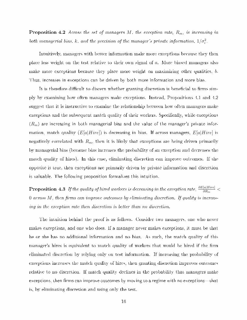
Proposition 4.2 Across the set of managers M , the exception rate, Rm, is increasing in

both managerial bias, k, and the precision of the manager's private information, 1/σ2ε .

Intuitively, managers with better information make more exceptions because they then

place less weight on the test relative to their own signal of a. More biased managers also

make more exceptions because they place more weight on maximizing other qualities, b.

Thus, increases in exceptions can be driven by both more information and more bias.

It is therefore di�cult to discern whether granting discretion is bene�cial to �rms sim-

ply by examining how often managers make exceptions. Instead, Propositions 4.1 and 4.2

suggest that it is instructive to examine the relationship between how often managers make

exceptions and the subsequent match quality of their workers. Speci�cally, while exceptions

(Rm) are increasing in both managerial bias and the value of the manager's private infor-

mation, match quality (E[a|Hire]) is decreasing in bias. If across managers, E[a|Hire] is

negatively correlated with Rm, then it is likely that exceptions are being driven primarily

by managerial bias (because bias increases the probability of an exception and decreases the

match quality of hires). In this case, eliminating discretion can improve outcomes. If the

opposite is true, then exceptions are primarily driven by private information and discretion

is valuable. The following proposition formalizes this intuition.

Proposition 4.3 If the quality of hired workers is decreasing in the exception rate,∂E[a|Hire]

∂Rm<

0 across M , then �rms can improve outcomes by eliminating discretion. If quality is increas-

ing in the exception rate then discretion is better than no discretion.

The intuition behind the proof is as follows. Consider two managers, one who never

makes exceptions, and one who does. If a manager never makes exceptions, it must be that

he or she has no additional information and no bias. As such, the match quality of this

manager's hires is equivalent to match quality of workers that would be hired if the �rm

eliminated discretion by relying only on test information. If increasing the probability of

exceptions increases the match quality of hires, then granting discretion improves outcomes

relative to no discretion. If match quality declines in the probability that managers make

exceptions, then �rms can improve outcomes by moving to a regime with no exceptions�that

is, by eliminating discretion and using only the test.

16

5 Managerial Discretion

The model motivates the following empirical question: Is worker tenure increasing or

decreasing in the probability of an exception? If decreasing, then No Discretion improves

worker outcomes relative to Discretion, and if increasing then Discretion improves upon No

Discretion.

In order to implement this test, we must address the empirical challenge that �excep-

tions� in our data are driven not only by managerial type (bias and information) as in the

model, but also by other factors. For example, quality and size of the applicant pools may

vary systematically with manager or location quality. We discuss how we apply our theory

to the data in the next two subsections. We �rst de�ne an exception rate to normalize vari-

ation across pools that mechanically makes exceptions more or less likely. We then discuss

empirical speci�cations designed to limit remaining concerns.

5.1 De�ning Exceptions

Our data provides us with the test scores of applicants post-testing. We use this infor-

mation to de�ne an �applicant pool� as a group of applicants being considered by the same

manager for a job at the same location in the same month.25

We can then measure how often managers overrule the recommendation of the test by

either 1) hiring a yellow when a green had applied and is not hired, or 2) hiring a red when

a yellow or green had applied and is not hired. We de�ne the exception rate, for a manager

m at a location l in a month t, as follows.

Exception Ratemlt =Nhy ∗Nnh

g +Nhr ∗ (Nnh

g +Nnhy )

Maximum # of Exceptions(2)

Nhcolor and N

nhcolor are the number of hired and not hire applicants, respectively. These

variables are de�ned at the pool level (m, l, t) though subscripts have been suppressed for

notational ease.

25An applicant is under consideration if he or she applied in the last 4 months and had not yet been hired.Over 90% of workers are hired within 4 months of the date they �rst submitted an application.

17

The numerator of Exception Ratemlt counts the number of exceptions (or �order viola-

tions�) a manager makes when hiring, i.e., the number of times a yellow is hired for each

green that goes unhired plus the number of times a red is hired for each yellow and green

that goes unhired.

The number of exceptions in a pool depends on both the manager's choices and on

factors related to the applicant pool, such as size and color composition. For example,

if a pool has only green applicants, it is impossible to make an exception. Similarly, if the

manager hires all available applicants, then there can also be no exceptions. These variations

were implicitly held constant in our model, but need to be accounted for in the empirics.

To isolate the portion of variation in exceptions that are driven by managerial decisions,

we normalize the number of order violations by the maximum number of violations that could

occur, given the applicant pool that the recruiter faces and the number of hires. Importantly,

although propositions in Section 4 are derived for the probability of an exception, their proofs

hold equally for this de�nition of an exception rate.26

From Table 1, we have 4,209 applicant pools in our data consisting of, on average 268

applicants.27 On average, 19% of workers in a given pool are hired. Roughly 40% of all

applicants in a given pool receive a �green�, while �yellow� and �red� candidates make up

roughly 30%, each. The test score is predictive of whether or not an applicant is hired. In

the average pool, greens and yellows are hired at a rate of roughly 20%, while only 9% of

reds are hired. Still, managers very frequently make exceptions to test recommendations:

the exception rate in the average pool (the average applicant is in a pool where an exception

rate of) 24% of the maximal number of possible exceptions.

Furthermore, we see substantial variation in the extent to which managers actually

follow test recommendations when making hiring decisions.28 Figure 3 shows histograms of

the exception rate, at the application pool level, as well as aggregated to the manager and

26Results reported below are qualitatively robust to a variety of di�erent assumptions on functional formfor the exception rate.

27This excludes months in which no hires were made.28According to the data �rm, client �rms often told their managers that job test recommendations should

be used in making hiring decisions but gave managers discretion over how to use the test (though some �rmsstrongly discouraged managers from hiring red candidates).

18

location levels. The top panels show unweighted distributions, while the bottom panels show

distributions weighted by the number of applicants.

In all �gures, the median exception rate is about 20% of the maximal number of possible

exceptions. At the pool level, the standard deviation is also about 20 percentage points; at

the manager and location levels, it is about 11 percentage points. This means that managers

very frequently make exceptions and that some managers and locations consistently make

more exceptions than others.

5.2 Empirical Speci�cations

Proposition 4.3 examines the correlation between the exception rate and the realized

match quality of hires in the post-testing period:

Durationmlt = a0 + a1Exception Ratemlt +Xmltγ + δl + δt + εmlt (3)

The coe�cient of interest is a1. A negative coe�cient, a1 < 0, indicates that the match

quality of hires is decreasing in the exception rate, meaning that �rms can improve the

match quality of hires by eliminating discretion and relying solely on job test information.

In addition to normalizing exception rates to account for di�erences in applicant pool

composition, we estimate multiple version of Equation (3) that include location and time

�xed e�ects, client-year �xed e�ects, location-speci�c linear time trends, and detailed controls

for the quality and number of applicants in an application pool.

These controls are important because observed exception rates may be driven by factors

other than a manager's type (bias and information parameters). For example, some locations

may be inherently less desirable than others, attracting both lower quality managers and

lower quality applicants. In this case, lower quality managers may make more exceptions

because they are biased. At the same time, lower quality workers may be more likely to

quit or be �red. Both facts would be driven by unobserved location characteristics. Another

potential concern is that undesirable locations may have di�culty hiring green workers, even

conditional on them having applied. In our data, we cannot distinguish a green worker who

19

refuses a job o�er from one who was never o�ered the job. As long as these characteristics

are �xed or vary smoothly at the location-level, our controls absorb this variation.

A downside of including many �xed e�ects in Equation (3) is that it increases the ex-

tent to which our identifying variation is driven by pool-to-pool variation in the idiosyncratic

quality of applicants. To see why this is problematic, imagine an applicant pool with a par-

ticularly weak draw of green candidates. In this case, we would expect a manager to make

more exceptions, and, that the yellows and reds hired will perform better than the unhired

greens from this particular pool. However, they may not perform better than the typical

green hired by that manager. In this case, a manager could be using his or her discretion

to improve match quality, but exceptions will still be correlated with poor outcomes. That

is, when we identify o� of pool-to-pool variation in exception rates, we may get the counter-

factual wrong because exceptions are correlated with variation in unobserved quality within

color.

To deal with the concern that Equation (3) relies too much on pool-to-pool variation

in exception rates, we can aggregate exception rates to the manager- or location-level. Ag-

gregating across multiple pools removes the portion of exception rates that are driven by

idiosyncratic di�erences in the quality of workers in a given pool. The remaining variation�

di�erences in the average exception rate across managers or locations�is more likely to

represent exceptions made because of managerial type (bias and information). Doing so,

however, reduces the amount of within-location variation left in our explanatory variable,

making controlling for location �xed e�ects di�cult or impossible.

To accommodate aggregate exception rates, we expand our data to include pre-testing

worker observations. Speci�cally, we estimate whether the impact of testing, as described in

Section 3, varies with exception rates:

Durationmlt = b0 + b1Testinglt × Exception Ratemlt + b2Testinglt (4)

+Xmltγ + δl + δt + εmlt

Equation (4) estimates how the impact of testing di�ers when managers make excep-

tions. The coe�cient of interest is b1. Finding b1 < 0 indicates that making more exceptions

20

decreases the improvement that locations see from the implementation of testing, relative

to their pre-testing baseline. Because exception rates are not de�ned in the pre-testing pe-

riod (there are no test scores in the pre-period), there is no main e�ect of exceptions in the

pre-testing period, beyond that which is absorbed by the location �xed e�ects δl.

This speci�cation allows us to use the pre-testing period to control for location-speci�c

factors that might drive correlations between exception rates and outcomes. It also expands

the sample on which we estimate location-speci�c time trends. This allows us to use exception

rates that are aggregated to the manager- or location-level, avoiding small sample variation.29

Aggregating exception rates to the location level also helps remove variation generated by any

systematic assignment of managers to applicants within a location that might be correlated

with exception rates and applicant quality.30

To summarize, we test Proposition 4.3 with two approaches. First, we estimate the

correlation between pool-level exception rates and quality of hires across applicant pools.

Second, we estimate the di�erential impact of testing across pools with di�erent exception

rates of hires, where exception rates can be de�ned at the application pool, manager-, or

location-level. In Section 5.4, we describe additional robustness checks.

5.3 Results

To gain a sense of the correlation between exception rates and outcome of hires, we �rst

summarize the raw data by plotting both variables at the location level. Figure 4 shows a

scatter plot of the location-level average exception rate on the x-axis and the location-level

average tenure (log of completed duration) for workers hired post-testing on the y-axis. In

the �rst panel, each location has the same weight; in the second, locations with more precise

outcomes receive more weight.31 In both cases, we see a negative correlation between the

29We de�ne a time-invariant exception rate for managers (locations) that equals the average exceptionrate across all pools the manager (location) hired in (weighted by the number of applicants).

30It also helps us rule out any measurement error generated by the matching of applicants to HR managers(see Appendix A for details). This would be a problem if in some cases hiring decisions are made morecollectively, or with scrutiny from multiple managers, and these cases were correlated with applicant quality.

31Speci�cally we weight by the inverse variance of the error associated with the location-speci�c treatmente�ect of testing, upweighting locations with more precisely estimated treatment e�ects. We use this weightto maintain consistency with subsequent �gures, though results are similar when we weight by location sizeor by the inverse variance of the pre-testing location-speci�c average duration.

21

extent to which managers exercise discretion by hiring exceptions, and the match quality of

those hired.

The �rst two columns of Table 3 present the correlation between exception rates and

worker tenure. We use a standardized exception rate with mean 0 and standard deviation 1

and in this panel exception rates are de�ned at the pool level (based on the set of applicants

and hires a manager makes at a particular location in a given month).32

Column 1 contains our base speci�cation and indicates that a one standard deviation

increase in the exception rate of a pool is associated with a 5% reduction in completed

tenure for that group, signi�cant at the 5% level. The coe�cient is still sizeable in Column 2

which contains our full set of controls, though it does fall slightly in magnitude and become

insigni�cant.

The remaining columns of Table 3 examine how the impact of testing varies by the

extent to which managers make exceptions. Our main explanatory variable is the interaction

between the introduction of testing and a post-testing exception rate.

In Columns 3 and 4, we continue to use pool-level exception rates. The coe�cient on

the main e�ect of testing represents the impact of testing at the mean exception rate (since

the exception rate has been standardized). Including the full set of controls (Column 4),

we �nd that locations with the mean exception rate experience a 0.22 log point increase

in duration as a result of the implementation of testing, but that this e�ect is o�set by a

quarter (0.05) for each standard deviation increase in the exception rate, signi�cant at the

1% level.

In Columns 5-8, we aggregate exception rates to the manager- and location-level.33

Results are quite consistent, using these aggregations, and the di�erential e�ects are even

larger in magnitude. Managers and locations that tend to exercise discretion bene�t much

less from the introduction of testing. A one standard deviation increase in the exception

rate reduces the impact of testing by roughly half to two-thirds.34

32We have experimented with di�erent functional forms for the exception rate variable in both panels andobtained qualitatively similar results.

33We have 555 managers who are observed in an average of 18 pools each (average taken over all man-agers, unweighted). We have 111 locations with on average 87 pools each (average taken over all locations,unweighted).

34As we noted above, it is not possible to use these aggregated exceptions rates when examining thepost-testing correlation between exceptions and outcomes (as in columns 1 and 2) because they leave little

22

To better illustrate the variation underlying these results, we plot location-speci�c treat-

ment e�ects of testing on the location's average exception rate. Figure 5 plots these for both

an unweighted and a weighted sample based on the same weights described above. The

relationship is clearly negative, and does not look to be driven by any particular location.

We therefore �nd that the match quality of hires is lower for applicant pools, managers,

and locations with higher exception rates. It is worth emphasizing that with the controls for

the size and quality of the applicant pool, our identi�cation comes from comparing outcomes

of hires across managers who make di�erent numbers of exceptions when facing similar

applicant pools. Given this, di�erences in exception rates should be driven by a manager's

own weighting of his or her private preferences and private information. If managers were

making these decisions optimally from the �rm's perspective, we should not expect to see

(as we do in Table 3) that the workers they hire perform systematically worse. Based on

Proposition 4.3, we can infer then that exceptions are largely driven by managerial bias,

rather than private information, and these �rms could improve outcomes of hires by limiting

discretion.

5.4 Additional Robustness Checks

In this section we address several alternative explanations for our �ndings.

5.4.1 Quality of �Passed Over� Workers

There are several scenarios under which we might �nd a negative correlation between

overall exceptions and outcomes without biased managers. For example, as mentioned above,

managers may make more exceptions when green applicants in an applicant pool are idiosyn-

cratically weak. If yellow workers in these pools are weaker than green workers in our sample

on average, it will appear that more exceptions are correlated with worse outcomes even

though managers are making individual exceptions to maximize match quality. Similarly,

our results in Table 3 show that locations with more exceptions see fewer bene�ts from the

introduction of testing. An alternative explanation for this �nding is that high exception

or no variation within locations to also identify location �xed e�ects, which, as we have argued, are quiteimportant.

23

locations are ones in which managers have always had better information about applicants:

these locations see fewer bene�ts from testing because they simply do not need the test.

In these and other similar scenarios, it should still be the case that individual exceptions

are correct: a yellow hired as an exception should perform better than a green who is not

hired. To examine this, we would like to be able to observe the counterfactual performance

of all workers who are not hired. This would allow us to directly assess whether managers

make exceptions to reduce false negatives, the possibility that a great worker is left unhired

because he or she scored poorly on the test.

While we cannot observe the performance all non-hired greens, we can proxy for this

comparison by exploiting the timing of hires. Speci�cally, we compare the performance of

yellow workers hired as exceptions to green workers from the same applicant pool who are

not hired that month, but who subsequently begin working in a later month. If it is the

case that managers are making exceptions to increase the match quality of workers, then the

exception yellows should have longer completed tenures than the �passed over" greens.

Table 4 shows that is not the case. The �rst panel compares individual durations

by restricting our sample to workers who are either exception yellows, or greens who are

initially passed over but then subsequently hired, and including an indicator for being in the

latter group. Because these workers are hired at di�erent times, all regressions control for

hire year-month �xed e�ects to account for mechanical di�erences in duration. For the last

column, which includes applicant pool �xed e�ects, the coe�cient on being a passed over

green compares this group to the speci�c yellow applicants who were hired before them.35

The second panel of Table 4 repeats this exercise, comparing red workers hired as exceptions

(the omitted group), against passed over yellows and passed over greens.

In both panels, we �nd that workers hired as exceptions have shorter tenures. Column

3 is our preferred speci�cation because it adds controls for applicant pool �xed e�ects. This

means we compare the green (and yellow) applicants who were passed over one month but

eventually hired, to the actual yellow (red) applicants hired �rst. We �nd that passed over

greens stay about 8% longer than the yellows hired before them in the same pool (top panel

35Recall that an applicant pool is de�ned by a manager-location-date. Applicant pool �xed e�ects thussubsume a number of controls from our full speci�cation in from Table 3

24

Column 3) and greens and yellows stay almost 19% and 12% longer, respectively, compared

to the reds they were passed over for.

The results in Table 4 mean that it is unlikely that exceptions are driven by better

information. When workers with better test scores are at �rst passed over and then later

hired, they still outperform the workers chosen �rst.36

Table 5 provides additional evidence that workers with longer gaps between application

date and hire date (which we treat as temporarily passed over applicants) are not simply ones

who were delayed because of better outside options. If this were the case, we would expect

these workers to have better outcomes once they do begin work. In Table 5, we compare

match quality for workers hired immediately (the omitted category), compared to those who

waited one, two, or three months before starting, holding constant test score. Because these

workers are hired at di�erent times, all regressions again control for hire year-month �xed

e�ects. Across all speci�cations, we �nd no signi�cant di�erences between these groups. If

anything we �nd for greens and yellows that were hired with longer delays have shorter job

spells than immediate hires. We thus feel more comfortable interpreting the workers with

longer delays as having been initially passed over.

Table 5 also provides insights about how much information managers have, beyond the

job test. If managers have useful private information about workers, then we would expect

them to be able to distinguish quality within test-color categories: greens hired �rst should

be better than greens who are passed up. Table 5 shows that this does not appear to be

the case. We estimate only small and insigni�cant di�erences in tenure, within color, across

start dates. That is, within color, workers who appear to be a manager's �rst choice do not

perform better than workers who appear to be a manager's last choice. This again suggests

the value of managerial private information is small, relative to the test.

5.4.2 Extreme Outcomes

We have thus far assumed that the �rm would like managers to maximize the average

match quality of hired workers. Firms may instead instruct managers to take a chance on

36An alternative explanation is that the applicants with higher test scores were not initially passed up,but were instead initially unavailable because of better outside options. However, we think this is unlikelyto be driving our results, given a strong desire by client �rms to �ll slots and training classes quickly.

25

candidates with poor test scores to avoid missing out on an exceptional hire. This could

explain why managers hire workers with lower test score candidates to the detriment of

average match quality; managers may be using discretion to minimize false negatives.37

Alternatively, �rms may want managers to use discretion to minimize the chance of hiring a

worker who leaves immediately.

The �rst piece of evidence that managers do not e�ectively maximize upside or minimize

downside is the fact, already shown, that workers hired as perform worse than the very

workers they were originally passed over. To address this more directly, Appendix Table A2

repeats our analysis focusing on performance in the tails, using the 90th and 10th percentiles

of log completed durations for a cohort as the dependent variables. These results show that

more exceptions imply worse performance even among top hires, suggesting managers who

make many exceptions are also unsuccessful at �nding star workers. We also show that more

exceptions decrease the performance of the 10th percentile of completed durations as well.

5.4.3 Heterogeneity across Locations

Another possible concern is that the usefulness of the test varies across locations and

that this drives the negative correlation between exception rates and worker outcomes. Our

results on individual exceptions already suggest that this is not the case. However, we explore

a couple of speci�c stories here.

As we have already noted, a location with very good private information pre-testing

would have both a high exception rate and a low impact of testing. If exceptions were

driven by information, rather than mistakes or bias, we should see that higher exception

rate locations were more productive pre-testing. However, Figure 6 plots the relationship

between a location's eventual exception rates and the match quality of its hires prior to the

introduction of testing, and shows no systematic relationship between the two.38

Alternatively, in very undesirable locations, green applicants might have better outside

options and be more di�cult to retain. In these locations, a manager attempting to avoid

costly retraining may optimally decide to make exceptions in order to hire workers with lower

37For example, Lazear (1998) points out that �rms may be willing to pay a premium for risky workers.38We maintain the same weighting as 5 so the two �gures are comparable.

26

outside options. Here, a negative correlation between exceptions and performance would not

necessarily imply that �rms could improve productivity by relying more on testing. However,

we see no evidence that the �return� to test score varies across locations. For example, when

we split locations by pre-testing worker durations (Appendix Table A3) or by exception rates

post-testing (Appendix Table A4) we see no systematic di�erences in the correlation between

test score and job duration of hired workers.

5.4.4 Productivity

Our results show that �rms can improve the match quality of their workers, as measured

by duration, by relying more on job test recommendations. Firms may not want to pursue

this strategy, however, if their HR managers exercise discretion in order to improve worker

quality on other metrics. For example, managers may optimally choose to hire workers who

are more likely to turn over if their private signals indicate that those workers might be more

productive while they are employed.

Our �nal set of results provides evidence that this is unlikely to be the case. Speci�cally,

for a subset of 62,494 workers (one-quarter of all hires) in 6 client �rms, we observe a direct

measure of worker productivity: output per hour.39 We are unable to reveal the exact nature

of this measure but some examples may include: the number of data items entered per hour,

the number of standardized tests graded per hour, and the number of phone calls completed

per hour. In all of these examples, output per hour is an important measure of e�ciency and

worker productivity. Our particular measure has an average of roughly 8 with a standard

deviation of roughly 5.

Table 6 repeats our main �ndings, using output per hour instead of job duration as

the dependent variable. We focus on estimates only using our base speci�cation (controlling

for date and location �xed e�ects) because the smaller sample and number of clients makes

identifying the other controls di�cult.40

Column 1 examines the impact of the introduction of testing, which we �nd leads to a

statistically insigni�cant increase of 0.7 transactions in an hour, or a roughly 8% increase.

39We have repeated our main analyses on the subsample of workers that have output per hour data andobtained similar results.

40Results are, however, qualitatively similar with additional controls, except where noted.

27

The standard errors are such that we can rule out virtually any negative impact of testing

on productivity with 90% con�dence.41

Column 2 documents the post-testing correlation between pool-level exceptions and

output per hour, and Columns 3-5 examine how the impact of testing varies by exception

rates. In all cases, we �nd no evidence that managerial exceptions improve output per hour.

Instead, we �nd noisy estimates indicating that worker quality appears to be lower on this

dimension as well. For example, in Column 2, we �nd a tiny, insigni�cant positive coe�cient

describing the relationship between exceptions and output. Taking it seriously implies that

a 1 standard deviation increase in exception rates is correlated with 0.07 more transactions,

or a less than 1% increase. In, Columns 3-5, we continue to �nd an overall positive e�ect of

testing on output; we �nd no evidence of a positive correlation between exception rates and

the impact of testing. If anything, the results suggest that locations with more exceptions

experience slightly smaller impacts of testing. These e�ects are insigni�cant.

Taken together, the results in Table 6 provide no evidence that exceptions are positively

correlated with productivity. This refutes the hypothesis that, when making exceptions,

managers optimally sacri�ce job tenure in favor of workers who perform better on other

quality dimensions.

6 Conclusion

We evaluate the introduction of a hiring test across a number of �rms and locations for

a low-skill service sector job. Exploiting variation in the timing of adoption across locations

within �rms, we show that testing increases the durations of hired workers by about 15%.

We then document substantial variation in how managers use job test recommendations.

Some managers tend to hire applicants with the best test scores while others make many

more exceptions. Across a range of speci�cations, we show that the exercise of discretion

(hiring against the test recommendation) is associated with worse outcomes.

41This result is less robust to adding additional controls, however we can still rule out that testing has asubstantial negative e�ect. For example, adding location-speci�c time trends, the coe�cient on testing fallsfrom 0.7 to 0.26 (with a standard error of about 0.45).

28

Our paper contributes a new methodology for evaluating the value of discretion in �rms.

Our test is intuitive, tractable, and requires only data that would readily be available for

�rms using workforce analytics. In our setting it provides the stark recommendation that

�rms would do better to remove discretion of the average HR manager and instead hire based

solely on the test. In practice, our test can be used as evidence that the typical manager

underweights the job test relative to what the �rm would prefer. Based on such evidence,

�rms may want to explore a range of alternative options, for example, allowing managers

some degree of discretion but limiting the frequency with which they can overrule the test,

or, adopt other policies to in�uence manager behavior such as direct pay for performance or

selective hiring and �ring.

These �ndings highlight the role new technologies can play in reducing the impact

of managerial mistakes or biases by making contractual solutions possible. As workforce

analytics becomes an increasingly important part of human resource management, more work

needs to be done to understand how such technologies interact with organizational structure

and the allocation of decisions rights with the �rm. This paper makes an important step

towards understanding and quantifying these issues.

29

References

[1] Aghion, Philippe and Jean Tirole (1997), �Formal and Real Authority in Organizations,�

The Journal of Political Economy, 105(1).

[2] Altonji, Joseph and Charles Pierret (2001), �Employer Learning and Statistical Discrim-

ination,� Quarterly Journal of Economics, 113: pp. 79-119.

[3] Alonso, Ricardo and Niko Matouschek (2008), �Optimal Delegation," The Review of

Economic Studies, 75(1): pp 259-3.

[4] Autor, David (2001), �Why Do Temporary Help Firms Provide Free General Skills

Training?,� Quarterly Journal of Economics, 116(4): pp. 1409-1448.

[5] Autor, David and D. Scarborough (2008), �Does Job Testing Harm Minority Workers?

Evidence from Retail Establishments,� Quarterly Journal of Economics, 123(1): pp.

219-277.

[6] Baker, George and Thomas Hubbard (2004), �Contractibility and Asset Ownership:

On-Board Computers and Governance in U.S. Trucking,� Quarterly Journal of Eco-

nomics, 119(4): pp. 1443-1479.

[7] Bolton, Patrick and Mathias Dewatripont (2010) �Authority in Organizations." in

Robert Gibbons and John Roberts (eds.), The Handbook of Organizational Eco-

nomics. Princeton, NJ: Princeton University Press.

[8] Brown, Meta, Elizabeth Setren, and Giorgio Topa (2015),�Do Informal Referrals Lead

to Better Matches? Evidence from a Firm's Employee Referral System,� Journal of

Labor Economics, forthcoming.

[9] Burks, Stephen, Bo Cowgill, Mitchell Ho�man, and Michael Housman (2015), �The

Value of Hiring through Employee Referrals,� Quarterly Journal of Economics,

130(2): pp. 805-839.

[10] Dana, Jason, Robyn Dawes, and Nathaniel Peterson (2013), �Belief in the Unstructured

Interview: The Persistence of an Illusion", Judgment and Decision Making, 8(5), pp.

512-520.

30

[11] Dessein, Wouter (2002) �Authority and Communication in Organizations," Review of

Economic Studies. 69, pp. 811-838.

[12] Farber, Henry. and Robert Gibbons (1996), �Learning and Wage Dynamics,� Quarterly

Journal of Economics, 111: pp. 1007-1047.

[13] Horton, John (2013), �The E�ects of Subsidizing Employer Search," mimeo New York

University.

[14] Jovanovic, Boyan (1979), "Job Matching and the Theory of Turnover," The Journal of

Political Economy, 87(October), pp. 972-90.

[15] Kahn, Lisa and Fabian Lange (2014), �Employer Learning, Productivity and the Earn-

ings Distribution: Evidence from Performance Measures,� Review of Economic Stud-

ies, 81(4) pp.1575-1613.

[16] Kahneman, Daniel (2011). Thinking Fast and Slow. New York: Farrar, Strauss, and

Giroux.

[17] Kuncel, Nathan, David Klieger, Brian Connelly, and Deniz Ones (2013), �Mechanical

Versus Clinical Data Combination in Selection and Admissions Decisions: A Meta-

Analysis," Journal of Applied Psychology. Vol. 98, No. 6, 1060�1072.

[18] Kuziemko, Ilyana (2013), �How Should Inmates Be Released from Prison? an Assess-

ment of Parole Versus Fixed Sentence Regimes," Quarterly Journal of Economics.

Vol. 128, No. 1, 371�424.

[19] Lazear, Edward P. (1998), �Hiring Risky Workers.� In Internal Labour Market, Incen-

tives, and Employment, edited by Isao Ohashi and Toshiaki Tachibanaki. New York:

St. Martin's.

[20] Lazear, Edward, Kathryn Shaw, and Christopher Stanton (2015), �The Value of Bosses,�

Journal of Labor Economics, forthcoming.

[21] Li, Danielle. (2012), �Expertise and Bias in Evaluation: Evidence from the NIH� mimeo

Harvard University.

31

[22] Oyer, Paul and Scott Schaefer (2011), �Personnel Economics: Hiring and Incentives,� in

the Handbook of Labor Economics, 4B, eds. David Card and Orley Ashenfelter, pp.

1769-1823.

[23] Pallais, Amanda and Emily Sands (2015), �Why the Referential Treatment? Evidence

from Field Experiments on Referrals,� The Journal of Political Economy, forthcom-

ing.

[24] Paravisini, Daniel and Antoinette Schoar (2013) �The Incentive E�ect of IT: Random-

ized Evidence from Credit Committees� NBER Working Paper #19303.

[25] Riviera, Lauren. (2014) �Hiring as Cultural Matching: The Case of Elite Professional

Service Firms.� American Sociological Review. 77: 999-1022

[26] Stanton, Christopher and Catherine Thomas (2014), �Landing The First Job: The Value

of Intermediaries in Online Hiring,� mimeo London School of Economics.

32

Figure 1: Distribution of Length of Completed Job Spells0

.002

.004

.006

.008

Dens

ity

0 200 400 600 800 1000Days of Tenure

Omits 3.7% of observations with durations over 1000 daysRed Line=Mean, Black line=Median

®Notes: Figure 1 plots the distribution of completed job spells at the individual level.

33

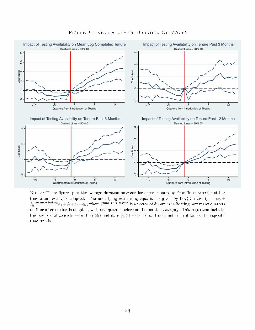
Figure 2: Event Study of Duration Outcomes

-.50

.51

1.5

2C

oeffi

cien

t

-10 -5 0 5 10Quarters from Introduction of Testing

Dashed Lines = 90% CIImpact of Testing Availability on Mean Log Completed Tenure

-.10

.1.2

.3C

oeffi

cien

t

-10 -5 0 5 10Quarters from Introduction of Testing

Dashed Lines = 90% CIImpact of Testing Availability on Tenure Past 3 Months

-.20

.2.4

Coe

ffici

ent

-10 -5 0 5 10Quarters from Introduction of Testing

Dashed Lines = 90% CIImpact of Testing Availability on Tenure Past 6 Months

-.20

.2.4

.6C

oeffi

cien

t

-10 -5 0 5 10Quarters from Introduction of Testing

Dashed Lines = 90% CIImpact of Testing Availability on Tenure Past 12 Months

Notes: These �gures plot the average duration outcome for entry cohorts by time (in quarters) until or

time after testing is adopted. The underlying estimating equation is given by Log(Duration)lt = α0 +

Itime since testinglt α1+ δl+γt+ εlt, where I

time since testing is a vector of dummies indicating how many quarters

until or after testing is adopted, with one quarter before as the omitted category. This regression includes

the base set of controls � location (δl) and date (γt) �xed e�ects; it does not control for location-speci�c

time trends.

34

Figure 3: Distributions of Application Pool Exception Rates0

.05

.1.1

5.2

0 .2 .4 .6 .8 1

Pool Level, Unweighted

0.0

5.1

.15

0 .2 .4 .6 .8 1

Pool Level, Weighted by # Applicants

0.0

5.1

.15

.2

0 .2 .4 .6 .8 1

Manager Level, Unweighted

0.1

.2.3

0 .2 .4 .6 .8 1

Manager Level, Weighted by # Applicants

0.0

5.1

.15

0 .2 .4 .6

Location Level, Unweighted

0.0

5.1

.15

.2

0 .2 .4 .6

Location Level, Weighted by # Applicants

Red Line=Mean, Black line=Median

®Notes: These �gures plot the distribution of the exception rate, as de�ned by Equation (2) in Section 5.

The leftmost panel presents results at the applicant pool level (de�ned to be a manager�location�month).

The middle panel aggregates these data to the manager level and the rightmost panel aggregates further to

the location level. Exception rates are only de�ned for the post-testing sample.

35

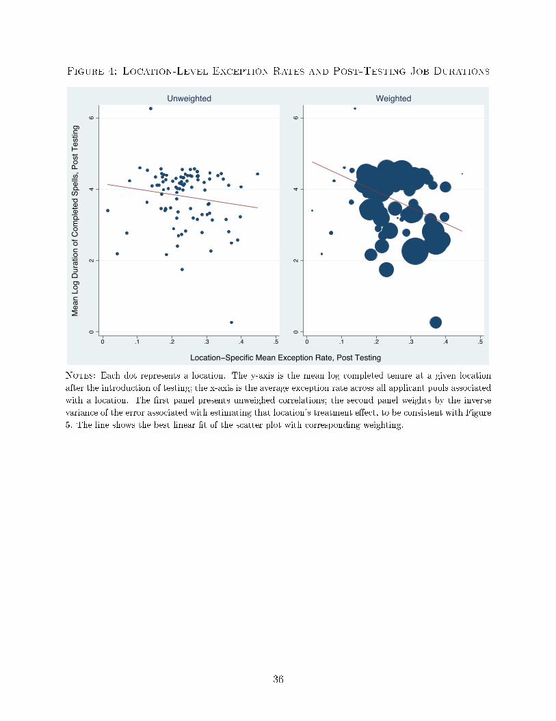
Figure 4: Location-Level Exception Rates and Post-Testing Job Durations

02

46

0 .1 .2 .3 .4 .5

Unweighted

02

46

0 .1 .2 .3 .4 .5

Weighted

Mea

n Lo

g D

urat

ion

of C

ompl

eted

Spe

lls, P

ost T

estin

g

Location−Specific Mean Exception Rate, Post Testing®

Notes: Each dot represents a location. The y-axis is the mean log completed tenure at a given location

after the introduction of testing; the x-axis is the average exception rate across all applicant pools associated

with a location. The �rst panel presents unweighed correlations; the second panel weights by the inverse

variance of the error associated with estimating that location's treatment e�ect, to be consistent with Figure

5. The line shows the best linear �t of the scatter plot with corresponding weighting.

36

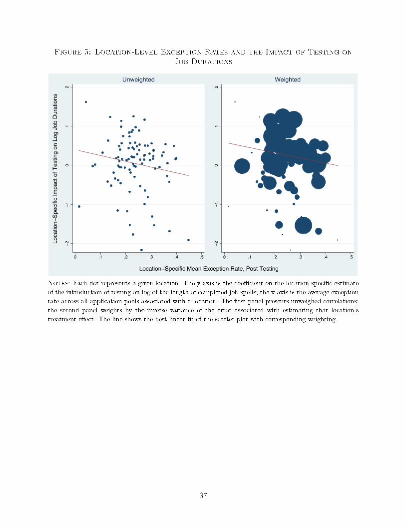
Figure 5: Location-Level Exception Rates and the Impact of Testing on

Job Durations−2

−10

12

0 .1 .2 .3 .4 .5

Unweighted

−2−1

01

2

0 .1 .2 .3 .4 .5

Weighted

Loca

tion−

Spec

ific

Impa

ct o

f Tes

ting

on L

og J

ob D

urat

ions

Location−Specific Mean Exception Rate, Post Testing®

Notes: Each dot represents a given location. The y-axis is the coe�cient on the location-speci�c estimate

of the introduction of testing on log of the length of completed job spells; the x-axis is the average exception

rate across all application pools associated with a location. The �rst panel presents unweighed correlations;

the second panel weights by the inverse variance of the error associated with estimating that location's

treatment e�ect. The line shows the best linear �t of the scatter plot with corresponding weighting.

37

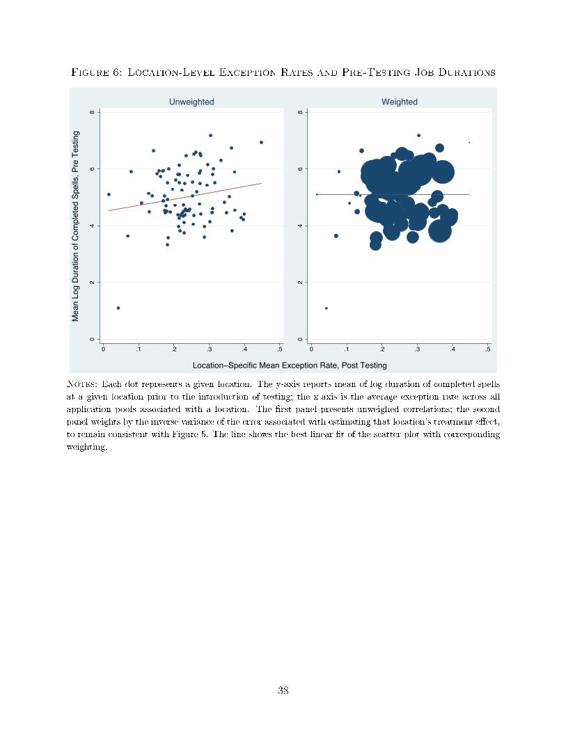
Figure 6: Location-Level Exception Rates and Pre-Testing Job Durations

02

46

8

0 .1 .2 .3 .4 .5

Unweighted

02

46

8

0 .1 .2 .3 .4 .5

Weighted

Mea

n Lo

g D

urat

ion

of C

ompl

eted

Spe

lls, P

re T

estin

g

Location−Specific Mean Exception Rate, Post Testing

®

Notes: Each dot represents a given location. The y-axis reports mean of log duration of completed spells

at a given location prior to the introduction of testing; the x-axis is the average exception rate across all

application pools associated with a location. The �rst panel presents unweighed correlations; the second

panel weights by the inverse variance of the error associated with estimating that location's treatment e�ect,

to remain consistent with Figure 5. The line shows the best linear �t of the scatter plot with corresponding

weighting.

38

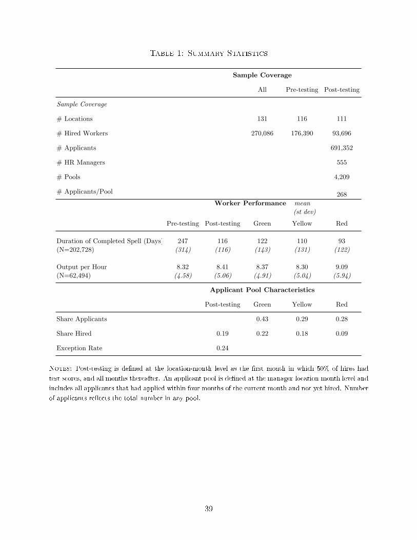
Table 1: Summary Statistics

All Pre-testing Post-testing

Sample Coverage

# Locations 131 116 111

# Hired Workers 270,086 176,390 93,696

# Applicants 691,352

# HR Managers 555

# Pools 4,209

# Applicants/Pool 268

Pre-testing Post-testing Green Yellow Red

Duration of Completed Spell (Days) 247 116 122 110 93(N=202,728) (314) (116) (143) (131) (122)

Output per Hour (N=62,494)

8.32(4.58)

8.41(5.06)

8.37(4.91)

8.30(5.04)

9.09(5.94)

Post-testing Green Yellow Red

Share Applicants 0.43 0.29 0.28

Share Hired 0.19 0.22 0.18 0.09

Exception Rate 0.24

Worker Performance mean (st dev)

Sample Coverage

Applicant Pool Characteristics

Notes: Only information on hired workers is available prior to the introduction of testing. Posttesting, there is information on applicants and hires. Post-testing is defined at the location-monthlevel as the first month in which 50% of hires had test scores, and all months thereafter. An applicantpool is defined at the hiring manager-location-month level and includes all applicants that had appliedwithin four months of the current month and not yet hired.

Notes: Post-testing is de�ned at the location-month level as the �rst month in which 50% of hires had

test scores, and all months thereafter. An applicant pool is de�ned at the manager-location-month level and

includes all applicants that had applied within four months of the current month and not yet hired. Number

of applicants re�ects the total number in any pool.

39

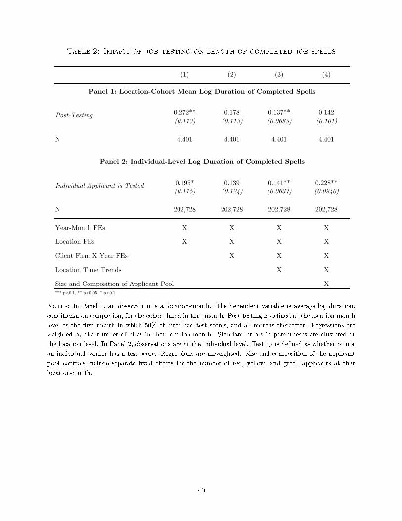
Table 2: Impact of job testing on length of completed job spells

(1) (2) (3) (4)

0.272** 0.178 0.137** 0.142(0.113) (0.113) (0.0685) (0.101)

N 4,401 4,401 4,401 4,401

0.195* 0.139 0.141** 0.228**(0.115) (0.124) (0.0637) (0.0940)

N 202,728 202,728 202,728 202,728

Year-Month FEs X X X X

Location FEs X X X X

Client Firm X Year FEs X X X

Location Time Trends X X

Size and Composition of Applicant Pool X

Individual Applicant is Tested

*** p<0.1, ** p<0.05, * p<0.1

Panel 2: Individual-Level Log Duration of Completed Spells

The impact of job testing on completed job spells

Post-Testing

Panel 1: Location-Cohort Mean Log Duration of Completed Spells

Notes: In Panel 1, an observation is a location-month. The dependent variable is average log duration,

conditional on completion, for the cohort hired in that month. Post-testing is de�ned at the location-month

level as the �rst month in which 50% of hires had test scores, and all months thereafter. Regressions are

weighted by the number of hires in that location-month. Standard errors in parentheses are clustered at

the location level. In Panel 2, observations are at the individual level. Testing is de�ned as whether or not

an individual worker has a test score. Regressions are unweighted. Size and composition of the applicant

pool controls include separate �xed e�ects for the number of red, yellow, and green applicants at that

location-month.

40

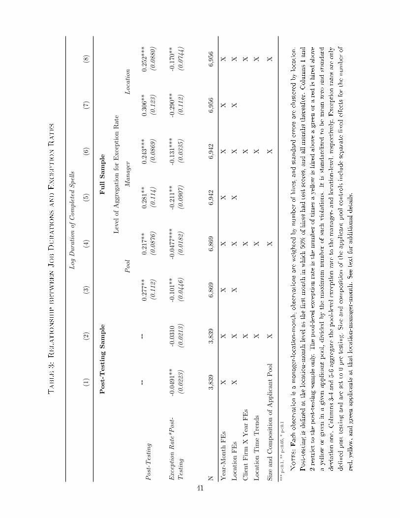
Table3:RelationshipbetweenJobDurationsandExceptionRates

(1)

(2)

(3)

(4)

(5)

(6)

(7)

(8)

----

0.27

7**

0.21

7**

0.28

1**

0.24

3***

0.30

6**

0.25

2***

(0.1

12)

(0.0

876)

(0.1

14)

(0.0

869)

(0.1

23)

(0.0

880)

-0.0

491*

*-0

.031

0-0

.101

**-0

.047

7***

-0.2

11**

-0.1

31**

*-0

.290

**-0

.170

**(0

.022

3)(0

.021

3)(0

.044

6)(0

.018

2)(0

.090

7)(0

.033

5)(0

.112

)(0

.074

4)

N3,

839

3,83

96,

869

6,86

96,

942

6,94

26,

956

6,95

6

Yea

r-M

onth

FE

sX

XX

XX

XX

X

Loca

tion

FE

sX

XX

XX

XX

X

Clie

nt F

irm

X Y

ear

FE

sX

XX

X

Loca

tion

Tim

e T

rend

sX

XX

X

XX

XX

Poo

lM

anag

erLo

cation

Rel

atio

nshi

p be

twee

n M

atch

Qua

lity

and

Exc

epti

on

Rat

es

Log

Dur

atio

n of

Com

plet

ed S

pells

Pos

t-Tes

ting

Sam

ple

Full S

ample

Leve

l of A

ggre

gation

for

Exc

eption

Rat

e

Pos

t-T

esting

Exc

eption

Rat

e*P

ost-

Tes

ting

Size

and

Com

posi

tion

of A

pplic

ant

Poo

l

***

p<0.

1, *

* p<

0.05

, * p

<0.

1

Notes:Each

observationisamanager-location-m

onth,observationsare

weightedbynumber

ofhires,andstandard

errors

are

clustered

bylocation.

Post-testingisde�ned

atthelocation-m

onth

levelasthe�rstmonth

inwhich50%

ofhires

hadtest

scores,andallmonthsthereafter.Columns1and

2restrict

tothepost-testingsampleonly.Thepool-levelexceptionrate

isthenumber

oftimes

ayellow

ishired

aboveagreen

oraredishired

above

ayellow

orgreen

inagiven

applicantpool,divided

bythemaximum

number

ofsuch

violations.

Itisstandardized

tobemeanzero

andstandard

deviationone.

Columns3-4

and5-6

aggregate

thepool-levelexceptionrate

tothemanager-andlocation-level,respectively.Exceptionratesare

only

de�ned

post

testingandare

setto

0pre

testing.Sizeandcompositionoftheapplicantpoolcontrolsincludeseparate

�xed

e�ects

forthenumber

of

red,yellow

,andgreen

applicants

atthatlocation-m

anager-m

onth.See

textforadditionaldetails.

41

Table 4: Match Quality of Exceptions vs. Passed Over Applicants

(1) (2) (3)

0.0436*** 0.0545*** 0.0794***(0.0140) (0.0118) (0.0236)

N 59,462 59,462 59,462

0.131*** 0.165*** 0.213***(0.0267) (0.0251) (0.0341)

0.0732*** 0.113*** 0.154***(0.0265) (0.0238) (0.0344)

N 44,456 44,456 44,456

Hire Month FEs X X X

Location FEs X X X

Full Controls from Table 3 X X

Application Pool FEs X

Quality of Exceptions vs. Passed over Applicants

Log Duration of Completed Spells

Passed Over Greens

Notes: Green are the omitted category

Panel 1: Quality of Yellow Exceptions vs. Passed over Greens

Panel 2: Quality of Red Exceptions vs. Passed over Greens and Yellows

Passed Over Greens

Passed Over Yellows

*** p<0.1, ** p<0.05, * p<0.1

Notes: Regressions are at the individual level on the post-testing sample. Standard errors are clustered by

location. Panel 1 includes yellow exceptions (who were hired when a green applicant was available but not

hired in that month) and passed over green applicants who were later hired. The omitted category are yellow

exceptions. The second panel includes red exceptions (who were hired when a green or yellow applicant was

available but not hired in that month) and passed over greens and yellows only. Red exceptions are the

omitted category. Application pool �xed e�ects are de�ned for a given location-manager-month.

42

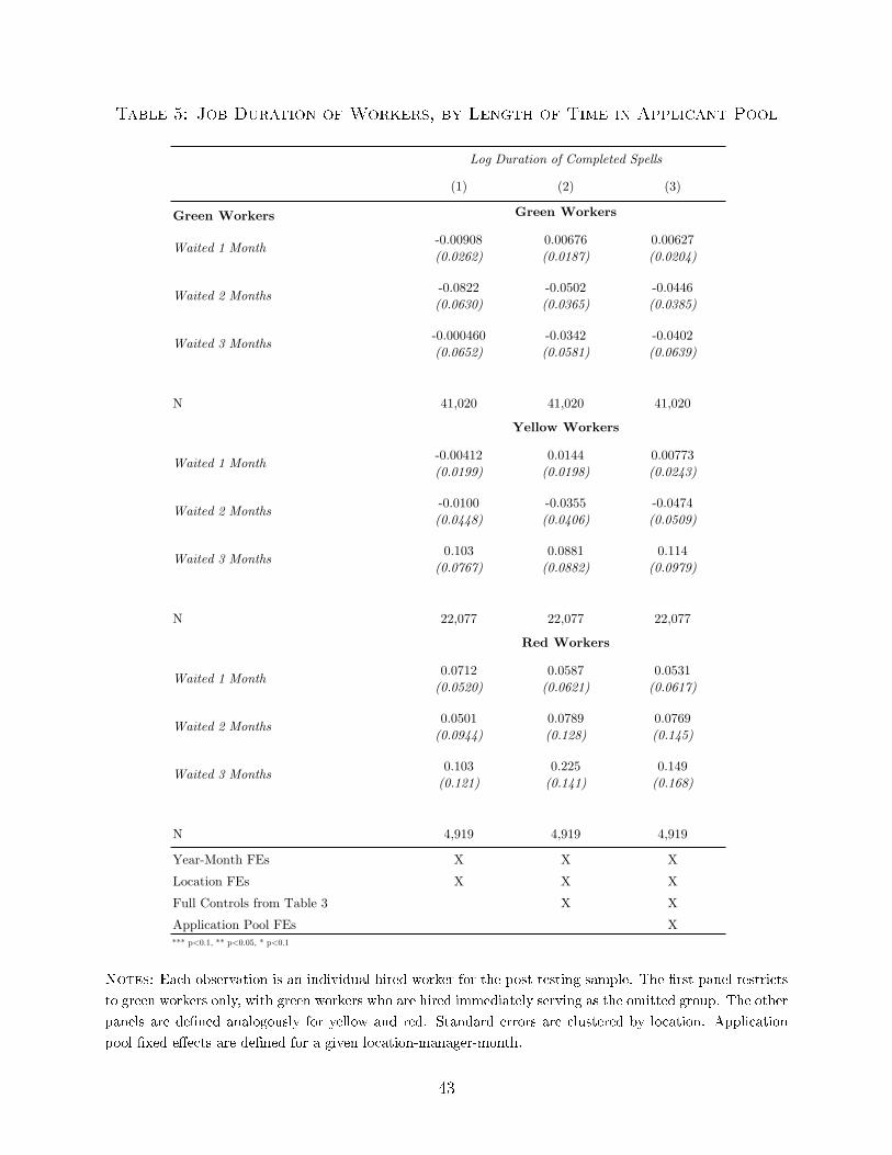
Table 5: Job Duration of Workers, by Length of Time in Applicant Pool

(1) (2) (3)

Green Workers

-0.00908 0.00676 0.00627(0.0262) (0.0187) (0.0204)

-0.0822 -0.0502 -0.0446(0.0630) (0.0365) (0.0385)

-0.000460 -0.0342 -0.0402(0.0652) (0.0581) (0.0639)

N 41,020 41,020 41,020

-0.00412 0.0144 0.00773(0.0199) (0.0198) (0.0243)

-0.0100 -0.0355 -0.0474(0.0448) (0.0406) (0.0509)

0.103 0.0881 0.114(0.0767) (0.0882) (0.0979)

N 22,077 22,077 22,077

0.0712 0.0587 0.0531(0.0520) (0.0621) (0.0617)

0.0501 0.0789 0.0769(0.0944) (0.128) (0.145)

0.103 0.225 0.149(0.121) (0.141) (0.168)

N 4,919 4,919 4,919

Year-Month FEs X X X

Location FEs X X X

Full Controls from Table 3 X X

Application Pool FEs X

Are Workers Who Start Later Better?

Log Duration of Completed Spells

Waited 1 Month

Waited 2 Months

Waited 3 Months

Green Workers

Yellow Workers

Red Workers

*** p<0.1, ** p<0.05, * p<0.1

Waited 1 Month

Waited 2 Months

Waited 3 Months

Waited 1 Month

Waited 2 Months

Waited 3 Months

Notes: Each observation is an individual hired worker for the post-testing sample. The �rst panel restricts

to green workers only, with green workers who are hired immediately serving as the omitted group. The other

panels are de�ned analogously for yellow and red. Standard errors are clustered by location. Application

pool �xed e�ects are de�ned for a given location-manager-month.

43

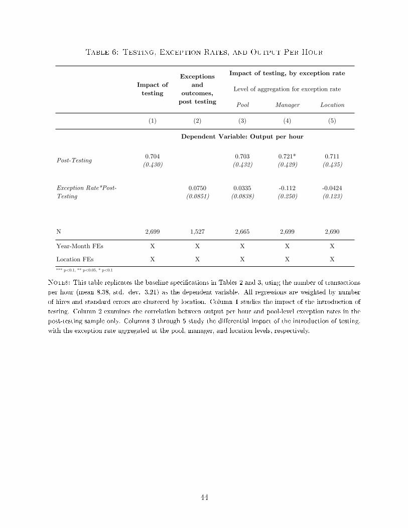
Table 6: Testing, Exception Rates, and Output Per Hour

Pool Manager Location

(1) (2) (3) (4) (5)

0.704 0.703 0.721* 0.711(0.430) (0.432) (0.429) (0.435)

0.0750 0.0335 -0.112 -0.0424(0.0851) (0.0838) (0.250) (0.123)

N 2,699 1,527 2,665 2,699 2,690

Year-Month FEs X X X X X

Location FEs X X X X X

*** p<0.1, ** p<0.05, * p<0.1

Post-Testing

Exception Rate*Post-Testing

Testing, Exceptions, and Number of Customers Served Per Hour

Impact of testing

Exceptions and

outcomes, post testing

Impact of testing, by exception rate

Level of aggregation for exception rate

Dependent Variable: Output per hour

Notes: This table replicates the baseline speci�cations in Tables 2 and 3, using the number of transactions

per hour (mean 8.38, std. dev. 3.21) as the dependent variable. All regressions are weighted by number

of hires and standard errors are clustered by location. Column 1 studies the impact of the introduction of

testing. Column 2 examines the correlation between output per hour and pool-level exception rates in the

post-testing sample only. Columns 3 through 5 study the di�erential impact of the introduction of testing,

with the exception rate aggregated at the pool, manager, and location levels, respectively.

44

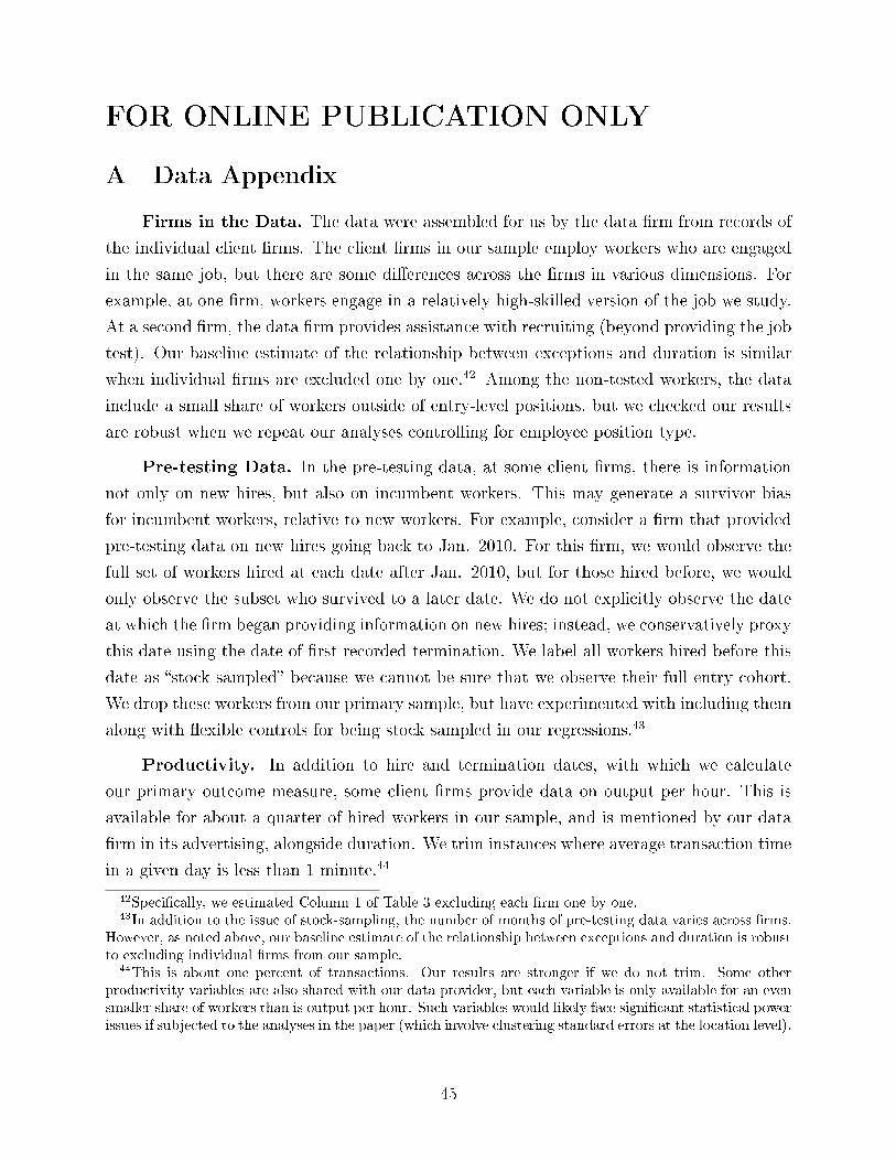
FOR ONLINE PUBLICATION ONLY

A Data Appendix

Firms in the Data. The data were assembled for us by the data �rm from records of

the individual client �rms. The client �rms in our sample employ workers who are engaged

in the same job, but there are some di�erences across the �rms in various dimensions. For

example, at one �rm, workers engage in a relatively high-skilled version of the job we study.

At a second �rm, the data �rm provides assistance with recruiting (beyond providing the job

test). Our baseline estimate of the relationship between exceptions and duration is similar

when individual �rms are excluded one by one.42 Among the non-tested workers, the data

include a small share of workers outside of entry-level positions, but we checked our results

are robust when we repeat our analyses controlling for employee position type.

Pre-testing Data. In the pre-testing data, at some client �rms, there is information

not only on new hires, but also on incumbent workers. This may generate a survivor bias

for incumbent workers, relative to new workers. For example, consider a �rm that provided

pre-testing data on new hires going back to Jan. 2010. For this �rm, we would observe the

full set of workers hired at each date after Jan. 2010, but for those hired before, we would

only observe the subset who survived to a later date. We do not explicitly observe the date

at which the �rm began providing information on new hires; instead, we conservatively proxy

this date using the date of �rst recorded termination. We label all workers hired before this

date as �stock sampled� because we cannot be sure that we observe their full entry cohort.

We drop these workers from our primary sample, but have experimented with including them

along with �exible controls for being stock sampled in our regressions.43

Productivity. In addition to hire and termination dates, with which we calculate

our primary outcome measure, some client �rms provide data on output per hour. This is

available for about a quarter of hired workers in our sample, and is mentioned by our data

�rm in its advertising, alongside duration. We trim instances where average transaction time

in a given day is less than 1 minute.44

42Speci�cally, we estimated Column 1 of Table 3 excluding each �rm one by one.43In addition to the issue of stock-sampling, the number of months of pre-testing data varies across �rms.

However, as noted above, our baseline estimate of the relationship between exceptions and duration is robustto excluding individual �rms from our sample.

44This is about one percent of transactions. Our results are stronger if we do not trim. Some otherproductivity variables are also shared with our data provider, but each variable is only available for an evensmaller share of workers than is output per hour. Such variables would likely face signi�cant statistical powerissues if subjected to the analyses in the paper (which involve clustering standard errors at the location level).

45

Test Scores. As described in the text, applicants are scored as Red, Yellow, or Green.

Applicants may receive multiple scores (e.g., if they are being considered for multiple roles).

In these cases, we assign applicants to the maximum of their scores.45

HR Manager. We do not have data on the characteristics of HR managers (we only

see an individual identi�er). When applicants interact with more than one HR manager

during the recruitment process, they are assigned to the manager with whom they have the

most interactions.46

In the data provided, information on HR manager is missing for about one-third of the

job-tested applicants. To form our base sample of workers in Table 1, we drop job-tested

workers where information on HR manager is missing. In forming our sample of applicants

and in creating the applicant pool variables, individuals with missing information on HR

manager are assigned to a separate category. We have also repeated our main analyses while

excluding all job-tested individuals (applicants and workers) where HR manager is missing

and obtained qualitatively similar results.

Race, Gender, Age. Data on race, sex, and age are not available for this project.

However, Autor and Scarborough (2008) show that job testing does not seem to a�ect worker

race, suggesting that changes in worker demographics such as race are not the mechanism

by which job testing improves durations.47

Location Identi�ers. In our dataset, we do not have a common identi�er for workplace

location for workers hired in the pre-testing period and applicants applying post-testing.

Consequently, we develop a crosswalk between anonymized location names (used for workers

in the pre-testing period) and the location IDs in the post-testing period. We drop workers

from our sample where the merge did not yield a clean location variable.48

Hiring Practices Information. For several client �rms, our data �rm surveyed its

account managers (who interact closely with the client �rms regarding job testing matters),

asking them to provide us with information on hiring practices once testing was adopted.

The survey indicated that �rms encouraged managers to hire workers with higher scores (and

some �rms had policies on not hiring low-scored candidates), but left substantial leeway for

45For 1 of the 15 �rms, the Red/Yellow/Green score is missing for non-hired applicants in the datasetprovided for this project. Our conclusions are substantively unchanged if that �rm is removed from thedata.

46This excludes interactions where information on the HR manager is missing. If there is a tie for mostinteractions, an applicant is assigned the last manager listed in the data among those tied for most interactionswith that applicant. Our main results are also qualitatively robust to setting the HR manager identi�er tomissing in cases of ties for most interactions.

47Autor and Scarborough (2008) do not look at impact of testing on gender. However, they show there islittle di�erential impact of testing by gender (or race).

48This includes locations in the pre-testing data where testing is never later introduced.

46

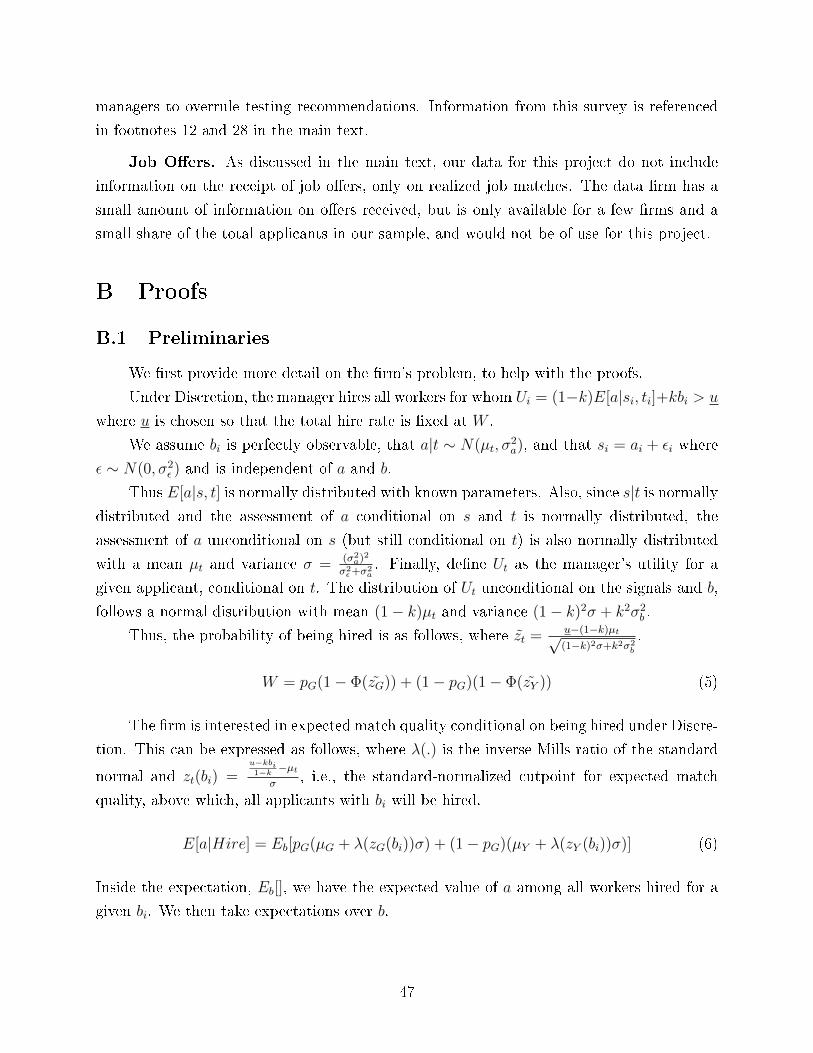
managers to overrule testing recommendations. Information from this survey is referenced

in footnotes 12 and 28 in the main text.

Job O�ers. As discussed in the main text, our data for this project do not include

information on the receipt of job o�ers, only on realized job matches. The data �rm has a

small amount of information on o�ers received, but is only available for a few �rms and a

small share of the total applicants in our sample, and would not be of use for this project.

B Proofs

B.1 Preliminaries

We �rst provide more detail on the �rm's problem, to help with the proofs.

Under Discretion, the manager hires all workers for whom Ui = (1−k)E[a|si, ti]+kbi > u

where u is chosen so that the total hire rate is �xed at W .

We assume bi is perfectly observable, that a|t ∼ N(µt, σ2a), and that si = ai + εi where

ε ∼ N(0, σ2ε ) and is independent of a and b.

Thus E[a|s, t] is normally distributed with known parameters. Also, since s|t is normally

distributed and the assessment of a conditional on s and t is normally distributed, the

assessment of a unconditional on s (but still conditional on t) is also normally distributed

with a mean µt and variance σ = (σ2a)2

σ2ε+σ2

a. Finally, de�ne Ut as the manager's utility for a

given applicant, conditional on t. The distribution of Ut unconditional on the signals and b,

follows a normal distribution with mean (1− k)µt and variance (1− k)2σ + k2σ2b .

Thus, the probability of being hired is as follows, where zt = u−(1−k)µt√(1−k)2σ+k2σ2

b

.

W = pG(1− Φ(zG)) + (1− pG)(1− Φ(zY )) (5)

The �rm is interested in expected match quality conditional on being hired under Discre-

tion. This can be expressed as follows, where λ(.) is the inverse Mills ratio of the standard

normal and zt(bi) =u−kbi1−k −µt

σ, i.e., the standard-normalized cutpoint for expected match

quality, above which, all applicants with bi will be hired.

E[a|Hire] = Eb[pG(µG + λ(zG(bi))σ) + (1− pG)(µY + λ(zY (bi))σ)] (6)

Inside the expectation, Eb[], we have the expected value of a among all workers hired for a

given bi. We then take expectations over b.

47

Under No Discretion, the �rm hires based solely on the test. Since we assume there are

plenty of type G applicants, the �rm will hire among type G applicants at random. Thus

the expected match quality of hires equals µG.

B.2 Proof of Proposition 3.1

The following results formalize conditions under which the �rm will prefer Discretion or No

Discretion.

1. For any given precision of private information, 1/σ2ε > 0, there exists a k′ ∈ (0, 1)

such that if k < k′ match quality is higher under Discretion than No Discretion and

the opposite if k > k′.

2. For any given bias, k > 0, there exists ρ such that when 1/σ2ε < ρ, i.e., when precision of

private information is low, match quality is higher under No Discretion than Discretion.

3. For any value of information ρ ∈ (0,∞), there exists a bias, k′′ ∈ (0, 1), such that

if k < k′′ and 1/σ2ε > ρ, i.e., high precision of private information, match quality is

higher under Discretion than No Discretion.

For this proof we make use of the following lemma:

Lemma B.1 The expected match quality of hires for a given manager, E[a|Hire], is de-

creasing in managerial bias, k.

Proof A manager will hire all workers for whom (1 − k)E[a|si, ti] + kbi > u, i.e., if bi >u−(1−k)E[a|si,ti]

k. Managers trade o� b for a with slope −1−k

k. Consider two managers, Manager

1 and Manager 2, where k1 > k2, i.e., Manager 1 is more biased than Manager 2. Manager

2 will have a steeper (more negative) slope (1−k2k2

> 1−k1k1

) than Manager 1. There will thus

be some cuto� a such that for E[a|si, ti] > a Manager 2 has a lower cuto� for b and for

E[a|si, ti] < a, Manager 1 has a lower cuto� for b.

That is, some candidates will be hired by both managers, but for E[a|si, ti] > a, Manager

2 (less bias) will hire some candidates that Manager 1 would not, and for E[a|si, ti] < a

Manager 1 (more bias) will hire some candidates that Manager 2 would not. The candidates

that Manager 2 would hire when Manager 1 would not, have high expected values of a, while

the candidates that Manager 1 would hire where Manager 2 would not have low expected

values of a. Therefore the average a value for workers hired by Manager 2, the less biased

manager, must be higher than that for those hired by Manager 1. E[a|Hire] is decreasingin k.

48

We next prove each item of Proposition 3.1

1. For any given precision of private information, 1/σ2ε > 0, there exists a k′ ∈ (0, 1)

such that if k < k′ match quality is higher under Discretion than No Discretion and

the opposite if k > k′.

Proof When k = 1, the manager hires based only on b, which is independent of a. So

E[a|Hire] = pGµG + (1 − pG)µY . The �rm would do better under No Discretion (where

match quality of hires equals µG). When k = 0, the manager hires only applicants whose

expected match quality, a, is above the threshold. In this case, the �rm will at least weakly

prefer Discretion. Since the manager's preferences are perfectly aligned, he or she will always

do at least as well as hiring only type G.

Thus, Discretion is better than No Discretion for k = 0 and the opposite is true for

k = 1. Lemma B.1 shows that the �rm's payo� is decreasing in k. There must therefore be

a single cutpoint, k′, where, below that point, the �rm's payo� for Discretion is large than

that for No Discretion, and above that point, the opposite is true.

2. For any given bias, k > 0, there exists ρ such that when 1/σ2ε < ρ, i.e., when precision of

private information is low, match quality is higher under No Discretion than Discretion.

Proof When 1/σ2ε = 0, i.e., the manager has no information, and k = 0, he or she will hire

based on the test, resulting in an equal payo� to the �rm as No Discretion. For all k > 0,

the payo� to the �rm will be worse than No Discretion, thanks to lemma B.1. Thus when

the manager has no information the �rm prefers No Discretion to Discretion.

We also point out that the �rm's payo� under Discretion, expressed above in equation

(6), is clearly continuous in σ (which is continuous in 1/σ2ε = 0).

Thus, when the manager has no information, the �rm prefers No Discretion and the

�rm's payo� under Discretion is continuous in the manager's information. Therefore there

must be a point ρ such that, for precision of manager information below that point, the �rm

prefers No Discretion to Discretion.

3. For any value of information ρ ∈ (0,∞), there exists a bias, k′′ ∈ (0, 1), such that

if k < k′′ and 1/σ2ε > ρ, i.e., high precision of private information, match quality is

higher under Discretion than No Discretion.

49

Proof First, we point out that when k = 0, the �rm's payo� under Discretion is increasing

in 1/σ2ε . An unbiased manager will always do better (from the �rm's perspective) with

more information than less. Second, we have already shown that for k = 0, Discretion is

always preferable to No Discretion, regardless of the manager's information, and when σ2ε

approached ∞, there is no di�erence between Discretion and No Discretion from the �rm's

perspective.

De�ne ∆(σ2ε , k) as the di�erence in match quality of hires under Discretion, compared

to no Discretion, for �xed manager type (σ2ε , k). We know that ∆(σ2

ε , 0) is positive and

decreasing in σ2ε , and approaches 0 as σ2

ε approaches ∞. Also, since the �rm's payo� un-

der discretion is continuous in both k and 1/σ2ε (see equation 6 above), ∆() must also be

continuous in these variables.

Fix any ρ and let σ2ε = 1/ρ. Let y = ∆(σ2

ε , 0). We know that ∆(σ2ε , 0) > y for all

σ2ε < σ2

ε .

Let d(k) = maxσ2ε∈[0,σ2

ε ]∆(σ2

ε , k)−∆(σ2ε , 0). We know d(k) exists because ∆() is continuous

wrt σ2ε and the interval over which we take the maximum is compact. We also know that

d(0) = 0, i.e., for an unbiased manager, the return to discretion is maximized when managers

have full information. Finally, d(k) is continuous in k because ∆() is.

Therefore, we can �nd k′′ > 0 such that d(k) = d(k)− d(0) < y whenever k < k′′. This

means that ∆(σ2ε , k) > 0 for σ2

ε < σ2ε . In other words, at bias k and ρ > ρ, Discretion is

better than No Discretion.

B.3 Proof of Proposition 3.2

Across M , the exception rate, Rm, is increasing in both managerial bias, k, and the precision

of the manager's private information, 1/σ2ε

Proof Because the hiring rate is �xed at W , E[Hire|Y ] is a su�cient statistic for the

probability that an applicant with t = Y is hired over an applicant with t = G, i.e., an

exception is made.

Above, we de�ned Ut, a manager's utility of a candidate conditional on t, and showed

that it is normally distributed with mean (1 − k)µt and variance Σ = (1 − k)2σ + k2σ2b . A

manager will hire all applicants for whom Ut is above u where the latter is chosen to keep

the hire rate �xed at W .

Consider the di�erence in expected utility across G and Y types. If µG − µY were

smaller, more Y types would be hired, while fewer G types would be hired. This is because,

at any given quantile of UG, there would be more Y types above that threshold.

50

Let us now de�ne Ut = Ut√Σ. This transformation is still normally distributed but now

has mean (1−k)µt√Σ

and variance 1. This rescaling of course does nothing to the cuto� u, and

it will still be the case that the probability of an exception is decreasing in the di�erence in

expected utilities across UG and UY : ∆U = (1−k)(µG−µY )√Σ

.

It is easy to show (with some algebra) that ∂∆U∂k

=−(µG−µY )σ2

b

Σ3/2 , which is clearly negative.

When k is larger, the expected gap in utility between a G and a Y narrows so the probability

of hiring a Y increases.

Similarly, it is each to show that ∂∆U∂σ2ε

= (1−k)3(µG−µY )(σ2a)2

2Σ3/2(σ2ε+σ2

a)2, which is clearly positive. The

gap in expected utility between G and Y widens when managers have less information. It

thus narrows when managers have better private information, as does the probability of an

exception.

B.4 Proof of Proposition 3.3

If the quality of hired workers is decreasing in the exception rate,∂E[a|Hire]

∂Rm< 0 across M ,

then �rms can improve outcomes by eliminating discretion. If quality is increasing in the

exception rate then discretion is better than no discretion.

Proof Consider a manager who makes no exceptions even when given discretion: Across a

large number of applicants, this only occurs if this manager has no information and no bias.

Thus the quality of hires by this manager is the same as that of hires under a no discretion

regime, i.e., hiring decisions made solely on the basis of the test. Compare outcomes for this

manager to one who makes exceptions. If ∂E[a|Hire]∂Rm

< 0, then the quality of hired workers

for the latter manager will be worse than for the former. Since the former is equivalent

to hires under no discretion, it then follows that the quality of hires under discretion will

be lower than under no discretion. If the opposite is true and the manager who made

exceptions, thereby wielding discretion, has better outcomes, then discretion improves upon

no discretion.

51

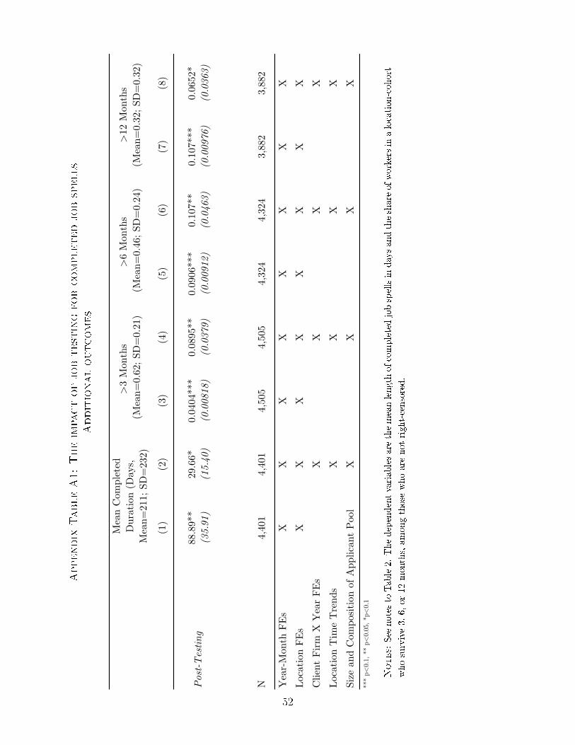
Appendix

TableA1:Theimpactofjobtestingforcompletedjobspells

Additionaloutcomes

(1)

(2)

(3)

(4)

(5)

(6)

(7)

(8)

88.8

9**

29.6

6*0.

0404

***

0.08

95**

0.09

06**

*0.

107*

*0.

107*

**0.

0652

*(35.91)

(15.40)

(0.00818)

(0.0379)

(0.00912)

(0.0463)

(0.00976)

(0.0363)

N4,

401

4,40

14,

505

4,50

54,

324

4,32

43,

882

3,88

2

Yea

r-M

onth

FE

sX

XX

XX

XX

X

Loca

tion

FE

sX

XX

XX

XX

X

Clie

nt F

irm

X Y

ear

FE

sX

XX

X

Loca

tion

Tim

e T

rend

sX

XX

X

XX

XX

***

p<0.

1, *

* p<

0.05

, *p<

0.1

Not

es: S

ee t

able

2. T

he d

epen

dent

var

iabl

e is

the

sha

re o

f w

orke

rs in

a lo

cation

-coh

ort

who

sur

vive

3, 6

, or

12 m

onth

s, a

mon

g th

ose

who

are

not

rig

ht-c

enso

red.

>6

Mon

ths

(M

ean=

0.46

; SD

=0.

24)

>12

Mon

ths

(Mea

n=0.

32; S

D=

0.32

)

The

impa

ct o

f jo

b te

stin

g f

or

compl

eted

job

spel

ls, A

ddit

iona

l O

utco

mes

Post-Testing

>3

Mon

ths

(M

ean=

0.62

; SD

=0.

21)

Mea

n C

ompl

eted

Dur

atio

n (D

ays,

M

ean=

211;

SD

=23

2)

Size

and

Com

posi

tion

of A

pplic

ant

Poo

l

Notes:See

notes

toTable2.Thedependentvariablesare

themeanlength

ofcompletedjobspellsindaysandtheshare

ofworkersinalocation-cohort

whosurvive3,6,or12months,amongthose

whoare

notright-censored.

52

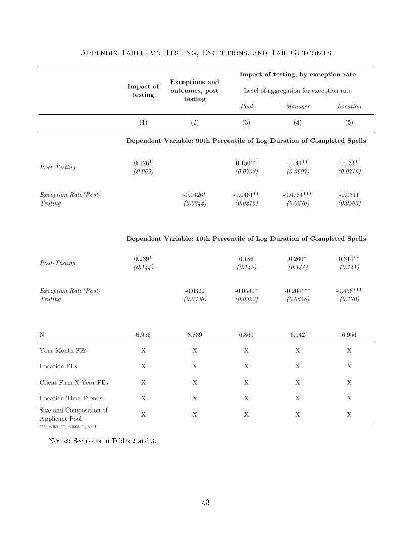
Appendix Table A2: Testing, Exceptions, and Tail Outcomes

Pool Manager Location

(1) (2) (3) (4) (5)

0.126* 0.150** 0.141** 0.131*(0.069) (0.0703) (0.0697) (0.0716)

-0.0426* -0.0461** -0.0764*** -0.0311(0.0242) (0.0215) (0.0270) (0.0563)

0.239* 0.186 0.260* 0.314**(0.144) (0.145) (0.144) (0.141)

-0.0322 -0.0540* -0.204*** -0.456***(0.0336) (0.0322) (0.0658) (0.170)

N 6,956 3,839 6,869 6,942 6,956

Year-Month FEs X X X X X

Location FEs X X X X X

Client Firm X Year FEs X X X X X

Location Time Trends X X X X X

Size and Composition of Applicant Pool

X X X X X

*** p<0.1, ** p<0.05, * p<0.1

Post-Testing

Exception Rate*Post-Testing

Dependent Variable: 10th Percentile of Log Duration of Completed Spells

Post-Testing

Exception Rate*Post-Testing

Dependent Variable: 90th Percentile of Log Duration of Completed Spells

Testing, Exceptions, and Tail Outcomes

Impact of testing

Exceptions and outcomes, post

testing

Impact of testing, by exception rate

Level of aggregation for exception rate

Notes: See notes to Tables 2 and 3.

53

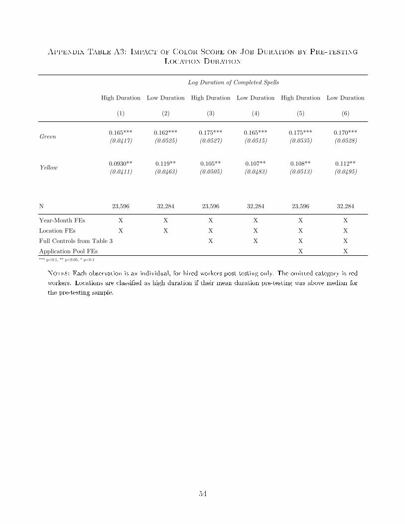
Appendix Table A3: Impact of Color Score on Job Duration by Pre-testing

Location Duration

High Duration Low Duration High Duration Low Duration High Duration Low Duration

(1) (2) (3) (4) (5) (6)

0.165*** 0.162*** 0.175*** 0.165*** 0.175*** 0.170***(0.0417) (0.0525) (0.0527) (0.0515) (0.0535) (0.0528)

0.0930** 0.119** 0.105** 0.107** 0.108** 0.112**(0.0411) (0.0463) (0.0505) (0.0483) (0.0513) (0.0495)

N 23,596 32,284 23,596 32,284 23,596 32,284

Year-Month FEs X X X X X X

Location FEs X X X X X X

Full Controls from Table 3 X X X X

Application Pool FEs X X

Information Content of Scores by Pre-Testing Duration

*** p<0.1, ** p<0.05, * p<0.1

Notes: Green are the omitted category

Log Duration of Completed Spells

Green

Yellow

Notes: Each observation is an individual, for hired workers post testing only. The omitted category is red

workers. Locations are classi�ed as high duration if their mean duration pre-testing was above median for

the pre-testing sample.

54

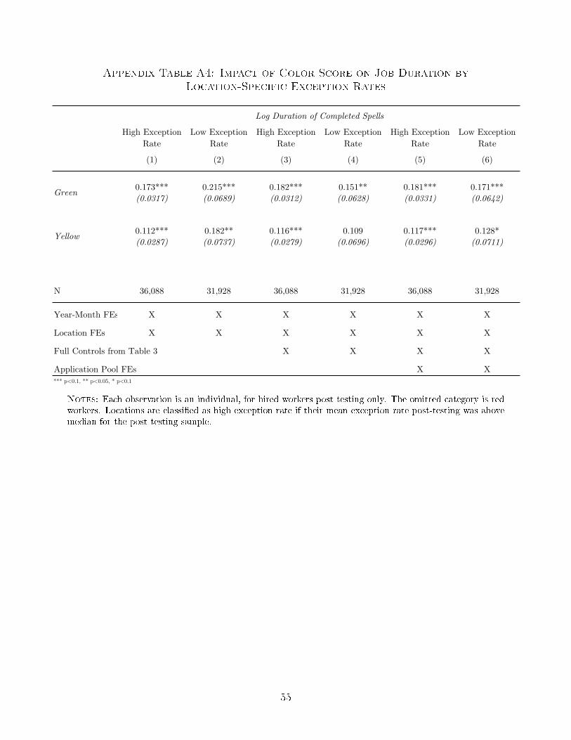
Appendix Table A4: Impact of Color Score on Job Duration by

Location-Specific Exception Rates

High Exception Rate

Low Exception Rate

High Exception Rate

Low Exception Rate

High Exception Rate

Low Exception Rate

(1) (2) (3) (4) (5) (6)

0.173*** 0.215*** 0.182*** 0.151** 0.181*** 0.171***(0.0317) (0.0689) (0.0312) (0.0628) (0.0331) (0.0642)

0.112*** 0.182** 0.116*** 0.109 0.117*** 0.128*(0.0287) (0.0737) (0.0279) (0.0696) (0.0296) (0.0711)

N 36,088 31,928 36,088 31,928 36,088 31,928

Year-Month FEs X X X X X X

Location FEs X X X X X X

Full Controls from Table 3 X X X X

Application Pool FEs X X

Score info by exception rate

*** p<0.1, ** p<0.05, * p<0.1

Notes: Green are the omitted category

Log Duration of Completed Spells

Green

Yellow

Notes: Each observation is an individual, for hired workers post testing only. The omitted category is redworkers. Locations are classi�ed as high exception rate if their mean exception rate post-testing was abovemedian for the post-testing sample.

55