Discretized Marching Cubes

C. Montani‡, R. Scateni?, R. Scopigno†

‡ I.E.I. – Consiglio Nazionale delle Ricerche, Via S. Maria 46, 56126 Pisa, ITALY

? Centro di Ricerca, Sviluppo e Studi Superiori Sardegna (CRS4), Cagliari, ITALY

† CNUCE – Consiglio Nazionale delle Ricerche , Via S. Maria 36, 56126 Pisa, ITALY

Abstract

Since the introduction of standard techniques for isosur-face extraction from volumetric datasets, one of the hardestproblems has been to reduce the number of triangles (orpolygons) generated.This paper presents an algorithm that considerably reducesthe number of polygons generated by a Marching Cubes-likescheme without excessively increasing the overall computa-tional complexity. The algorithm assumes discretization ofthe dataset space and replaces cell edge interpolation bymidpoint selection. Under these assumptions, the extractedsurfaces are composed of polygons lying within a finite num-ber of incidences, thus allowing simple merging of the outputfacets into large coplanar polygons.An experimental evaluation of the proposed approach ondatasets related to biomedical imaging and chemical mod-elling is reported.

1 Introduction

The use of the Marching Cubes (MC) technique, originallyproposed by W. Lorensen and H. Cline [7], is considered tobe a standard approach to the problem of extracting isosur-faces from a volumetric dataset. Marching Cubes is a verypractical and simple algorithm and many implementationsare available both as part of commercial systems or as pub-lic domain software.Despite its extensive use in many applications, it does havesome particular shortcomings: topological inconsistency [1],algorithm computational efficiency and excessive output datafragmentation. Standard MC produces no consistent notionof object connectivity; the local surface reconstruction crite-rion used give rise to a number of topological ambiguities,and therefore MC may output surfaces which are not neces-sarily coherent. These shortcomings have been extensivelystudied [11] and solutions have been proposed [12, 15, 8].MC computational efficiency can be increased by exploit-ing implicit parallelism (each cell can be independently pro-cessed) [4] and by avoiding the visiting and testing of empty

cells or regions of the volume [14].Excessive fragmentation of the output data can prevent in-teractive rendering when high resolution datasets are pro-cessed. What has changed since the technique was intro-duced seven years ago, has been the amount of data to beprocessed while extracting such surfaces. Equipments thatcan generate volumetric datasets as large as 512∗512∗[≤ 512]are now generally available, and we are on the way to achiev-ing machines capable of producing 1024 ∗ 1024 ∗ [≤ 1024]datasets or, in other words, 1 Gigavoxel per dataset. Al-though an isosurface does not usually cross all the voxels,we can understand how easy it is to generate more than onemillion triangles per surface. State-of-the-art hardware isnot yet fast enough to manipulate such masses of data inreal time.These obstacles gave rise to substantial research aimed atreducing the number of triangles generated by MC. The so-lutions proposed can be classified into adaptive techniques,where the cell size is locally adapted to the shape of the sur-face [10] or the dataset is organized into high and low inter-est areas and more primitives are produced in selected areasonly; and filtering techniques, where facet meshes returnedby a surface fitting algorithm are filtered in order to mergeor eliminate part of them.Filtering–based approaches can be classified as:

a) coplanar facets merging, in which facets are filtered bysearching for and merging coplanar and adjacent facets [6];

b) elimination of tiny facets, where the irregularity of thesurface produced is reduced by eliminating the tiny trian-gles produced when the iso-surface passes near a vertex oran edge of a cubic cell; this is accomplished by bending themesh so that a number of selected mesh nodes will lie on theiso–surface and the tiny triangles will degenerate into singlevertices. The solution is based on a modified iso-surface fit-ting algorithm and a filtering phase; 40% reductions in thenumber of triangles are reported [9];

c) approximated surface fitting, based on trading off datareduction for a reduction in the precision of the representa-tion generated, using error criteria to measure the suitabilityof the approximated surfaces.Schroeder et al. [13] proposed an algorithm based on mul-tiple filtering passes, that by analysing locally the geometryand topology of a triangle mesh removes vertices that passa minimal distance or curvature angle criterion. The advan-tage of this approach is that any level of reduction can beobtained, on the condition that a sufficiently coarse approx-

Figure 1: The set of different vertex locations produced byDiscMC.

imation threshold is set; reductions up to 90% have beenobtained with an approximation error lower than the voxelsize.In another approach, by Hoppe et al. [5], mesh optimiza-tion is achieved by evaluating an energy function over themesh, and then minimizing this function by either remov-ing/moving vertices or collapsing/swapping edges.Both approaches require a topological representation of themesh to be decimated.

In this work we propose Discretized Marching Cubes(DiscMC), an algorithm situated half-way between the cu-berille method, which assumes constant value voxels anddirectly returns the voxels faces (orthogonal to the volumeaxes) [3], and the cell interpolation approach of MC. On thebasis of two simple considerations, which both relate to datacharacteristics and visualization requirements, our solutionleads to interesting reductions in output fragmentation byapplying a very simple filtering approach. Moreover, theuse of an unambiguous triangulation scheme [8] allows iso-surfaces without topological anomalies to be obtained.

2 The Discretized Marching Cubes Algorithm

Given a binary dataset, linear interpolation is not neededto extract isosurfaces. When a cell edge in a binary datasethas both on and off corners, the midpoint of the edge is theintersection being looked for.In a number of applications where approximated isosurfacesmight be acceptable, the former assumption can be reason-ably extended to n–value high resolution datasets. The max-imal approximation error involved by adopting midpoint in-terpolation is 1/2 of the cell size, and in some applicationsthe resolution of the dataset justifies such a lack of preci-sion. Considering a 512 ∗ 512 ∗ [≤ 512] resolution, renderingthe isosurface generated produces approximately the sameimages whether linear interpolation or midpoint selection isused.

Discretized Marching Cubes (DiscMC) is here proposedas an evolution of MC based on midpoint selection. Theset of vertices that can be generated by DiscMC are shownin Figure 1: there are only 13 different spatial locations onwhich new vertices can be created (12 cell-edge midpointsplus the cell centroid). Moreover, applying midpoint selec-tion in MC allows for a finite set of planes where the gen-erated facets lie. We have only 13 different plane incidencesonto which a facet can lie, and these are described by thefollowing equations:

Figure 2: The facets returned by DiscMC for each differentplane incidence.

Figure 3: The sets of facets returned by DiscMC for eachcell vertex configuration.

x = c, y = c, z = c,

x± y = c, x± z = c, y ± z = c,

x± y ± z = c.

As shown in Figure 2, for each incidence the algorithm gen-erates a limited number of different facets.The following considerations are the basis of our DiscMCalgorithm:

a) each facet can be simply classified in terms of its shapeand plane incidence;

b) the limited number of different plane incidences increasesthe percentage of coplanar adjacent facets and thereforedrastically reduces the number of polygons returned whilepreserving small, but possibly significant, roughnesses;

c) the algorithm does not require interpolation of the surfaceintersections along the edges of the cells; this implies that itworks in integer arithmetic (except for the computation ofnormals) at a higher speed than standard methods.

2.1 A new lookup table

For each on-off combination of the cell vertices (there are256 different combinations), the standard MC lookup table(lut) codes the number of triangles produced and the celledges on which these vertices lie.DiscMC requires a simple reorganization of the standard MClut. Midpoint selection means that the number of differentfacets returned by DiscMC is fixed, and we only have a con-stant number of different output primitives for each plane

Figure 4: Some cell configurations and related DiscMClookup table entries.

incidence: only right triangles are generated on planes x = c,y = c and z = c (Figures 2.1, 2.2 and 2.3); only rectangles onplanes x± y = c, x± z = c and y ± z = c (Figures 2.4, 2.5,2.6, 2.7, 2.8 and 2.9); only equilateral triangles on planesx± y± z = c (Figures 2.10, 2.11, 2.12 and 2.13). Moreover,using midpoint interpolation means that the geometrical lo-cation of facet vertices depends solely on the vertices con-figuration and the position of the cell in the dataset mesh.Under these assumptions, the resulting facet set returnedby DiscMC for each of the canonical MC configurations isreported in Figure 3. With respect to the original proposalby Lorensen and Cline we omit configuration 14 (this can beobtained by reflection from configuration 11, i.e. configura-tion k in Figure 3.). Furthermore, three more configurationshave to be managed in order to prevent topological ambigu-ity (configurations n, o and p in Figure 3 [8]).Each facet is coded in the DiscMC lut by using a shape code,which codifies the shape and position of the facet (1..4 forright triangles, 1..2 for rectangles and 1..8 for equilateral tri-angles), and an incidence code, i.e. the plane on which thefacet lies. Geometrical information on the facet vertices isnot explicitly stored in the DiscMC lut.For each cell vertex configuration, DiscMC lut stores fromzero up to seven facets, each represented by a shape code(1..8) and an incidence code (-13..13). We use signed inci-dences to store separately facets which lie on the same planeand have opposite normals direction (both in order to givean implicit representation of facet orientation and to fastfacet search in the postprocessing merging phase).Some cell configurations are graphically represented in Fig-ure 4, together with the corresponding DiscMC lut entries.

2.2 Isosurface extraction

The isosurface reconstruction process returns intermediateresults using a set of indexed data structures. The volumedataset is processed slice by slice. For each cell traversedby an isosurface, the DiscMC produces a set of facets by

means of the DiscMC lut. Each facet is coded by its shape,incidence and the index of the cell in which it lies (i.e. itsgeometical position).In order to optimize the merging phase the facets producedare stored in a number of hash tables, one for each differentincidence of the facets. Thus, 26 hash tables are used, andhash indexes are computed in terms of shape code and cellindex.

2.3 Post-processing merging phase

The merging phase begins when the isosurfaces have beenfitted. Each hash table is analyzed in order to search foradjacent faces, which by construction of the hash tables willalso be iso-oriented and mergeable. Hash coding is chosento allow a rapid search for adjacent facets (a nearly constantmean access time has been measured in a number of algo-rithm runs).The merging algorithm does not work with the vertex co-ordinates of each merging polygon, but adopts Freeman’schains [2] as an intermediate representation scheme. In thisscheme, a polygonal line is represented by the coordinatesof the starting point of the chain and a set of directed links,that is, a set of relative displacements. This solution allowsthe unnecessary vertices to be rapidly eliminated.

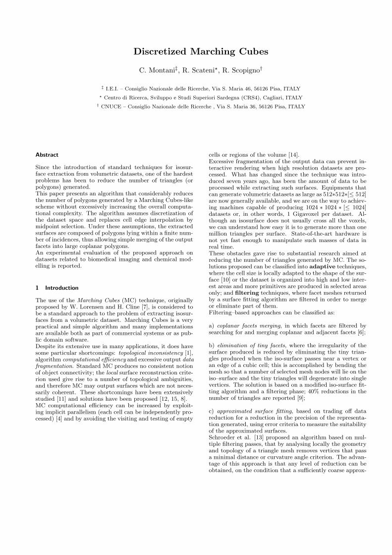
The merging algorithm is simple and efficient. Due tothe limited number of facet shapes and orientations, for eachfacet f and for each edge e of f the facet f ′ which might beadjacent on e to f is univocally determined. The algorithmis outlined in Figure 5 (an example is shown in Figure 6).

PUSH∗ verifies, for each edge pushed onto the edgestack,if an opposite edge exists on the stack, i.e. an edge with thesame geometrical position but moving in the opposite direc-tion. If this edge exists, mark both the edges as connectingedges. Marked edges will produce either connecting links(i.e. links which connect the starting point of the chain tothe boundary of the region, or the boundary of the regionto the boundary of the holes; see links 2 and 7 in the 15thtiles triple of Figure 6), or consecutive opposite links thathave to be eliminated due to the reconstruction algorithmadopted.

The Merge algorithm main loop iterates until hash tablesare empty. For each iteration of the first while loop, Mergeproduces the boundary of a region (anticlockwise in our im-plementation) and the boundaries of the holes (clockwise),if any. At the end of each iteration the boundaries of regionsand holes are reconstructed by eliminating the marked linksand, if necessary, by splitting the chain. Chains are thenconverted in the usual vertex–based representation.

The Merge algorithm uses a set of simple lookup tableswhich permit a general procedure to be designed irrespectiveof the type of the facets and the plane they belong to. Theselookup tables store:

• the edges to be pushed onto the edgestack (dependingon the starting point chosen);

• the edges to be pushed onto the edgestack when anadjacent facet has been found, or otherwise the link tobe added to the Freeman’s chain;

• the position (with respect to the current cell) of thecells to be inspected for adjacent facets.

In addition, through lookup tables we convert the chain linksinto relative displacements depending on the incidence planewe are examining.

Figure 7: The links of Freeman’s chains for (a) right trian-gles belonging to plane 3, (b) rectangles of plane 9, and (c)equilateral triangles of plane 12.

As previously introduced, with Freeman’s chain representa-tion scheme (Figure 7 shows the links used for three types ofelementary primitives) unnecessary vertices can be removedby simply converting equal consecutive links into a singlesegment.The worst case computational complexity of the mergingphase is linear to the number of facets returned by the iso-surface reconstructor. For each edge, the merger computesthe potential adjacent facet and searches for such a facet inthe hash table (a nearly constant time operation). In theworst case, when no mergeable facet pairs exist, the test isrepeated e times for each facet f , with e the number of edgesof facet f .

2.4 Vertex normals computation

Normals on the vertices of the isosurfaces extracted areneeded in order to compute Gouraud or Phong shading.Normals can be computed during isosurface extraction (interms of gradients [16], as in standard MC) or after themerging phase. In the current DiscMC implementation wecomputed vertex normals at the end of the merging processin order to avoid computing and storing a lot of unnecessaryvertex normals. However, further processing of the volumedata is thus needed.

3 Evaluation of results and conclusions

We tested DiscMC on a series of different datasets and com-pared results with a classic MC implementation. Table 1 re-ports the number of polygons generated and it refers to threedatasets: Sphere is a voxelized sphere, Buckyball is theelectron density around a molecule of C60 (courtesy of AVSInternational Centre) and Head is a CAT scanned dataset(courtesy of of Niguarda Hospital, Milan, Italy). The num-bers of facets and vertices returned by Classic MC and Dis-cMC are reported in Table 1. DiscMC returns triangular(3 − facets), quadrilateral (4 − facets) or n-sided facets

Algorithm MERGEinput HT1, ..., HT26:facet hash tables;output F :facet list;

beginfor each hash table HTi do

while HTi is not empty do• extract a facet f from hash table HTi;• select one of the vertices of f as the starting point of thecurrent Freeman chain;• push the edges of the facet onto the edgestack (LIFO);{each edge is coded in the edgestack by the shape code of the current facetand the shape code and the cell coordinates of the potential adjacent facet.This notation will indicate, for each edge extracted from edgestack,the source facet and the adjacent facet to be searched for.}while edgestack is not empty do

er:=POP(edgestack); {er:edge record}fadj :=er.adjacent facet;if facet fadj is contained in HTi

then• extract the facet fadj ;for each edge ej ∈ fadj such that ej 6= er do

PUSH∗(edgestack, ej); {PUSH∗: see text in Section 2.3}else

• add a link to the chain which is directed according to the current edge er;• if the edge is a connecting edge, add a marked link to the current chain(e.g. the link with a white arrow head in the 16th tile triple in Figure 6);

• insert the current Freeman chain into F ;end algorithm.

Figure 5: Pseudocode of the Merge algorithm

(n − facets); the respective numbers are in the rightmostthree columns in Table 1.

Time comparison needs to be split into three steps: facetextraction, merging and generation of normals. The per-centage of time spent in each stage of the computation variesfrom dataset to dataset; on average, it takes about 10% ofthe total time to extract facets, 85% to merge polygons, andabout 5% to generate normals. The buckyball dataset andthe head dataset, which are comparable in terms of voxelnumber, took around 2-3 minutes and 6-7 minutes, respec-tively, on an IBM RISC6000/550 workstation.

It is difficult to make a time comparison with other fil-tering approaches, because most of them do not report therunning times but only the simplification percentages ob-tained. The mesh optimization approach by Hoppe et al.[5] is the only alternative technique which reports runningtimes; the simplification of meshes (8000-18000 facets) withthis method, which produces very good results indeed, tooktens of minutes on a DEC Alpha workstation.In the proposal by Schroeder et al. [13] running times arenot reported, but the decimation phase is a much more com-plex task than the simple merging phase of DiscMC. In fact,the simplification of the mesh is obtained by multiple passesover the mesh. At each pass a vertex is selected for removal,all triangles that are incident on that vertex are removed,and the resulting hole is patched by computing a new localtriangulation.On the other hand, in the worst case, DiscMC has a com-plexity linear to the number of edges: for each edge of eachfacet, it searches for the adjacent facet on a hash list (aconstant time and cheap operation), and makes an inser-tion/removal onto/from the edge stack.The reduction in time complexity is significant, because the

design goal of DiscMC was to give simplified meshes withhigh efficiency, to be used, for example, while searching forthe correct threshold. Once this threshold has been selected,a more sophisticated method such as [13] can be used to ob-tain the best approximated mesh.

Another characteristic which differentiates DiscMC fromother simplification approaches is that it does not entailmanaging a geo-topological representation of the trianglemesh. The topological relations are implicitly stored in thecoding scheme used (facets shape and incidence) and thissimplifies the implementation at the cost of single constant–time search into hash lists.

The results obtained and the good quality of the outputimages (the colour plates in Figures 9 and 11 were obtainedwith our algorithm, while the ones on Figures 8 and 10 wereobtained with classic MC without mesh simplification) sup-port our claim that Discretized Marching Cubes representsa valid tool for the rapid reconstruction and visualization ofisosurfaces from medium and high resolution 3D datasets.One of the most salient characteristics of the algorithm isthat integer arithmetic is sufficient, and restricts the use offloating point computations to normals only. This is an im-portant factor which enhances the overall performance.Discretized Marching Cubes is both a valid solution for ap-plications where the precision of the result is not critical oralso as an intermediate solution to speed up the time neededto tune parameters, relegating to the final stage alone theuse of techniques that are more precise in terms of visualresults or geometrical approximation, such as ray tracing orstandard MC.

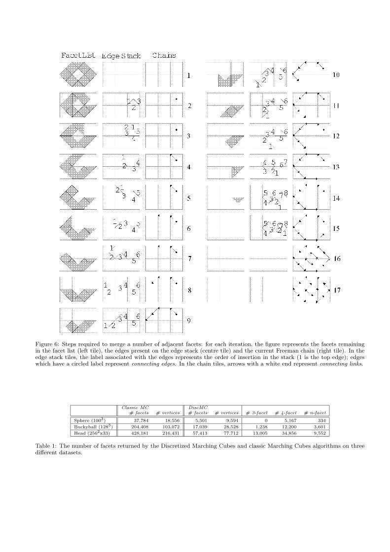
Figure 6: Steps required to merge a number of adjacent facets: for each iteration, the figure represents the facets remainingin the facet list (left tile), the edges present on the edge stack (centre tile) and the current Freeman chain (right tile). In theedge stack tiles, the label associated with the edges represents the order of insertion in the stack (1 is the top edge); edgeswhich have a circled label represent connecting edges. In the chain tiles, arrows with a white end represent connecting links.

Classic MC DiscMC# facets # vertices # facets # vertices # 3-facet # 4-facet # n-facet

Sphere (1003) 37,784 18,556 5,501 9,594 0 5,167 334

Buckyball (1283) 204,408 103,072 17,039 28,528 1,238 12,200 3,601

Head (2562x33) 428,181 216,431 57,413 77,712 13,005 34,856 9,552

Table 1: The number of facets returned by the Discretized Marching Cubes and classic Marching Cubes algorithms on threedifferent datasets.

4 Acknowledgements

This work has been partially carried out with the financialcontribution of the Sardinian Regional Authorities.

References

[1] M. J. Durst. Letters: Additional reference to “MarchingCubes. ACM Computer Graphics, 22(4):72–73, 1988.

[2] H. Freeman. Computer processing of line-drawing im-ages. ACM Computing Surveys, 6:57–97, 1974.

[3] D. Gordon and J.K. Udupa. Fast surface tracking in 3Dbinary images. Computer Vision, Graphics and ImageProcessing, (45):196–214, 1989.

[4] C.D. Hansen and P. Hinker. Massively parallel isosur-face extraction. In A.E. Kaufman and G.M. Nielson, ed-itors, Visualization ’92 Proceedings, pages 77–83. IEEEComputer Society Press, 1992.

[5] H. Hoppe, T. DeRose, T. Duchamp, J. McDonald,and W. Stuetzle. Mesh optimization. ACM ComputerGraphics (SIGGRAPH ’93 Conf. Proc.), pages 19–26,August 1-6 1993.

[6] A.D. Kalvin, C.B. Cutting, B. Haddad, and M.E. Noz.Constructing topologically connected surfaces for thecomprehensive analysis of 3D medical structures. SPIEVol. 1445 Image Processing, pages 247–259, 1991.

[7] W. Lorensen and H. Cline. Marching cubes: a high res-olution 3D surface construction algorithm. ACM Com-puter Graphics, 21(4):163–170, 1987.

[8] C. Montani, R. Scateni, and R. Scopigno. A modifiedlook-up table for implicit disambiguation of MarchingCubes. The Visual Computer, Vol.10, 1994, to appear.

[9] D. Moore and J. Warren. Compact isocontours fromsampled data. In D. Kirk, editor, Graphics Gems III,pages 23–28. Academic Press, 1992.

[10] H. Muller and M. Stark. Adaptive generation of sur-faces in volume data. The Visual Computer, 9(4):182–199, 1993.

[11] P. Ning and J. Bloomenthal. An Evaluation of ImplicitSurface Tilers. IEEE Computer Graphics & Applica-tions, 13(6):33–41, Nov. 1993.

[12] B.A. Payne and A.W. Toga. Surface mapping brainfunctions on 3D models. IEEE Computer Graphics &Applications, 10(2):41–53, Feb. 1990.

[13] W.J. Schroeder, J.A. Zarge, and W. Lorensen. Dec-imation of triangle mesh. ACM Computer Graphics,26(2):65–70, July 1992.

[14] J. Wilhelms and A. Van Gelder. Octrees for fasterisosurface generation. ACM Computer Graphics,24(5):57–62, Nov. 1990.

[15] J. Wilhelms and A. Van Gelder. Topological considera-tions in isosurface generation. ACM Computer Graph-ics, 24(5):79–86, Nov 1990.

[16] R. Yagel, D. Cohen, and A. Kaufman. Normal esti-mation in 3D discrete space. The Visual Computer,8:278–291, 1992.

Figure 8: Isosurface reconstruction from the Buckyballdataset using standard MC (no mesh simplification).

Figure 9: Isosurface reconstruction from the Buckyballdataset using DiscMC.

Figure 10: Isosurface reconstruction from the Head dataset using standard MC (no mesh simplification).

Figure 11: Isosurface reconstruction from the Head dataset using DiscMC.