Brigham Young UniversityDepartment of Electrical and Computer Engineering

459 Clyde BuildingProvo, Utah 84602

Microwave Earth Remote Sensing (MERS) Laboratory

Display and Computation of Windsin Oceanography and Meteorology

David G. Long, Ph.D.

22 Feb. 1994

MERS Technical Report # MERS 94-001ECEN Department Report # TR-L102-94.1

© Copyright 1994, Brigham Young University. All rights reserved.

Display and Computation of Winds in Oceanography and Meteorology

Dr. David G. LongMarch 16, 1994

Electrical and Computer Engineering Department459 Clyde Building, Brigham Young University, Provo, UT 84602

Abstract

This report describes standard plotting and display conventions for winds and wind-derived fields used inocean oceanography and meteorology. These are used to document plotting and computational algorithmsfor model-based wind field estimation. Emphasis is placed on computing the wind vorticity and diver-gence using mixed coordinate systems. Various examples using Seasat and ERS-1 scatterometer data arepresented.

1 Introduction: Conventions for Describing Winds

Plotting and displaying wind fields are a common need when studying wind fields and their derivatives.Unfortunately much confusion arises due to the fact that there are several standard ways or coventionsof plotting wind vector fields. This problem is complicated by the mixed coordinate systems which occurin scatterometry. Part of the purpose of this report is to clearly state these conventions and methods forconverting from one to another and to treat display and plotting the the presence of mixed coordinatesystems.

Separate conventions are used in meteorology and oceanography, with two frequently used conventionsin oceanography. A common convention is accepted for the component (u, v) winds.

1.1 Meteorological Convention

Flags (barbs) are most commonly used to denote the wind direction and wind speed. However, vectorsare also frequently used. When winds are plotted using vectors the direction of the arrow points towardthe direction from which the wind flows, i.e., the arrow acts like an anemometer. Directions are measuredclockwise (CW) from North. An angle of 0◦ denotes a Northerly wind flowing from North to South. Anangle of 270◦ denotes a Westerly wind flowing from West to East. In the meteorological convention, thehead of the arrow (i.e., the point) is displayed at the location of the measurement site. The tail extendsoutward from the measurement location.

1.2 Oceanographic Conventions

Unfortunately, two wind conventions for wind directions are used in oceanography. In both conventions,the arrow used to indicate the wind (or ocean) denotes the direction of mass flow. In the most commonconvention, wind angles are clockwise (CW) from North. A wind angle of 0◦ denotes a wind flowing fromthe South to the North and 90◦ denotes a wind flowing from West to East. Less commonly, the angle iscounter-clockwise (CCW) relative to East. In both conventions the base or tail of the arrow is located atthe measurement site with the head extending away from the measurement site.

1

1.3 Component Convention

Fortunately, the convention for the wind vector components is common to both arenas. A given wind vector~U may be decomposed into two orthogonal flow components, u and v, i.e., ~U = (u, v). u is known as thezonal wind and is positive toward the East. v is the meridonal wind and is positive to the North. Thus,u and v make up a standard right-handed x, y coordinate systems. In this system the wind direction iscounter-clockwise (CCW) from East so that a 0◦ wind denotes a zonal flow toward the East while a 90◦

wind denotes flow toward the North.

1.4 Hemispherical Flow

Given a weather map in which the convention is initially uncertain, the convention in use can be determinedby looking at the wind flow around sharp lows. In the Nothern hemisphere, such a flow is CCW while inthe Southern hemisphere it is CW.

1.5 Conversion Between Conventions

The meteorological convention and the primary oceanographic convention (relative to North) differ by 180◦.Derivatives in one consistent coordinate system will be the negative of consistent derivatives in the othersystem. For the oceanographic convention, given a wind speed S and a wind direction relative to North φo,the u and v component winds are computed as

φu = 90◦ − φo (1)u = S cos φu (2)v = S sinφu. (3)

For the meteorological convention with wind direction φm

φu = 90◦ − (φm − 180◦)= −φm − 90◦ (4)

u = −S cos φu (5)v = −S sinφu. (6)

To convert u and v component winds into oceanographic or meteorological convention wind speed anddirection,

φu = tan−1 v/u (four quadrant inverse) (7)

S =√

u2 + v2 (8)φo = 90◦ − φu (9)φm = −φu − 90◦. (10)

Note that none of these conversions are simple rotations.

2 Wind Coordinate Systems

Consider a two-dimension vector field ~V (x, y) with scalar component fields Vx(x, y) and Vy(x, y), i.e.,

~V (x, y) = Vx(x, y)x + Vy(x, y)y

2

where x and y are unit vectors in the x and y directions respectively.In this report, x will be aligned East-West (positive toward East) and y will be aligned North-South

(positive toward North) or (x, y) = (E, N). Thus, u = x, v = y, Vx(x, y)4= u(x, y) and Vy(x, y)

4= v(x, y)

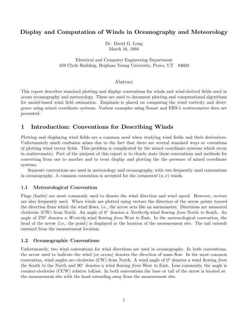
where the circumflex denotes a unit vector.Our measurements of ~V (x, y) are made over a swath aligned with a rotated coordinate system (x′, y′) as

shown in Fig. 1 for both ascending and descending orbits. The measurement system measures Vx(x, y) andVy(x, y). It is also capable of providing estimates of the partial derivatives; however, it can only estimatederivatives along the (c, a) axis system, i.e., along (x′, y′). The angle (always positive) between x and x′ isα = ψg. Note that for an ascending orbit x′ corresponds to c and y′ corresponds to a while for a descedingorbit x′ corresponds to −c and y′ corresponds to −a where the c, a axes indicate the cross-track/along-trackdata indexing.

α

Y

X

Y'

X'

ObservationSwath

α

Y

X

Y'

X'

ObservationSwath

S/C FlightDirection

S/C FlightDirection

Ascending Descending

c

ac

a

Figure 1: Rotational geometry

To express the component fields in the primed system as a function of the unprimed system using asimple rotational transformation as,

Vx′(x′, y′) = Vx(x, y) cos α + Vy(x, y) sinα (11)Vy′(x′, y′) = −Vx(x, y) sinα + Vy(x, y) cos α. (12)

Similarly,

Vx(x, y) = Vx′(x′, y′) cos α − Vy′(x′, y′) sinα (13)Vy(x, y) = Vx′(x′, y′) sinα + Vy′(x′, y′) cosα. (14)

These can be expressed in matrix form by first writting

~V =

[Vx(x, y)Vy(x, y)

](15)

and~V ′ =

[Vx′(x′, y′)Vy′(x′, y′)

](16)

3

Then,

~V ′ = T (α)~V (17)~V = T (−α)~V ′ (18)

where the 2 × 2 rotation matrix T (α) is defined as

T (α) =

[cosα sinα

− sinα cos α

]. (19)

To relate the primed (x′, y′) system to the cross/along-track (c, a) system,

Vx′(x′, y′) = δVc(c, a) (20)Vy′(x′, y′) = δVa(c, a) (21)

whereδ =

{1 ascending orbit−1 descending orbit.

(22)

In matrix form this is

~V † = T (δ′180◦)~V (23)~V = T (δ′180◦)~V † (24)

where~V † =

[Vc(c, a)Va(c, a)

](25)

andδ′ =

{0 ascending orbit1 descending orbit.

(26)

2.1 Mixed Coordinates

Suppose,that we begin with ~Vo = [uo, vo]t where

uo = S cos φo (27)vo = S sinφo. (28)

where S is the wind speed and φo is the oceanographic convention wind direction. What is the relationshipbetween ~Vo and ~V = [u, v]t?

Note that φu = 90◦ − φo and

u = S cos φu (29)v = S sinφu. (30)

We see that,

cosφu = cos(90◦ − φo)= cos(90◦) cosφo + sin(90◦) sinφo

= sinφo (31)sinφu = sin(90◦ − φo)

= sin(90◦) cos φo − cos(90◦) sinφo

= cosφo. (32)

4

It follows that the u and v components of the wind expressed in conventional coordinates are a transfor-mation of the uo and vo components, i.e., u = vo and v = uo,

~V =

[uv

]=

[0 11 0

] [uo

vo

]= R~Vo = −R~Vm. (33)

where ~Vm = [S cos φm, S sinφm]t = −~Vo. However, the transformation defined by R can not be expressedas a simple rotation, i.e., by T (α). Note that R is its own inverse, i.e., R = R−1.

2.2 Consistent Coordinates

To develop a consistent coordinate frame for model-based wind field estimation let us define the following:

φmbe = φu + δ′180◦ = 90◦ − φo + δ′180◦ = −90◦ − φm − δ′180◦ (34)

andφc = φu + δ′180◦ − δα = 90◦ − φo + δ′180◦ − δα = −90◦ − φm + δ′180◦ − δα. (35)

Then, φmbe gives the wind direction assuming that the along-track direction of scatterometer samplingswath (grid) is aligned with North-South and where the cross-track is aligned with East-West. This anglewill be used in place of φc whenever α is unavailable.

The angle φc is the rotation of the wind vector to the scatterometer sampling grid. The quantityuc = S cosφc is the projection of u onto the positive cross-track axis and vc = S sinφc is the projection ofv onto the along-track axis. Let ~Vc = [uc, vc]t and ~V = [u, v]t. We see that,

cosφc = cos(φu + δ′180◦ − δα)= cosφu cos(δ′180◦ − δα) − sinφu sin(δ′180◦ − δα)= cosφu

(cos δ′180◦ cos δα + sin δ′180◦ sin δα

)− sinφu

(sin δ′180◦ cos δα − cos δ′180◦ sin δα

)

= cosφuδ cos δα + sinφuδ sin δα

= δ (cos φu cos δα + sinφu sin δα) (36)

= δ (sinφo cos δα + cosφo sin δα) (37)sinφc = sin(φu + δ′180◦ − δα)

= sinφu cos(δ′180◦ − δα) + cos φu sin(δ′180◦ − δα)= sinφu

(cos δ′180◦ cos δα + sin δ′180◦ sin δα

)+ cosφu

(sin δ′180◦ cos δα − cos δ′180◦ sin δα

)

= sinφuδ cos δα − cosφuδ sin δα

= δ (sinφu cos δα − cos φu sin δα) (38)

= δ (cos φo cos δα − sinφo sin δα) (39)

It follows that

~Vc = δT (+δα)~V = δT (+δα)R~Vo = −δT (+δα)R~Vm (40)~V = δT (−δα)~Vc (41)~Vo = δRT (−δα)~Vc = −~Vm. (42)

Thus, φc is a simple rotation (and sign change for descending orbits) of the u, v component winds. As willbe shown below, this implies that the curl and divergence of ~Vc in the (c,a) system will be the same as thecurl and divergence of ~V in the (u,v) [i.e., (x,y)=(E,N)] coordinate system. (Note, however, that the signsof the curl and divergence of ~Vc must be reversed, or multiplied by δ, for a descending orbit.) Therefore,φc provides a consistent coordinate transform between (c,a) and (x,y).

5

3 Scatterometer Dataset Winds and Wind Retrieval

This section documents the conventions uses in processed winds, the geophysical model function relatingradar backscatter to winds, and the definitions of the relative the azimuth angle.

3.1 Wind Dataset conventions

Attached are plots for both ascending and descending passes using relative to North and MBE grid-relativeplots for SASS and ERS-1 winds. The AES/Woiceshyn SASS winds are in the meteorological convention.Atlas/GSFC SASS wind directions are given as clockwise from North. I believe these winds are also givenin the meteorlogical convention. ERS-1 scatterometer data (retrieved winds) is delivered from JPL (1993)in wind speed and direction. While the first data delieveries where identified as oceanographic convention,this was later corrected to be the meteorological convention with wind directions given with respect toNorth. Winds blowing from the West to the East have a direction of 90◦. NSCAT has chosen to representall winds in the oceanographic convention.

3.2 Wind Retrieval and the Geophysical Model Function

The geophysical model function (e.g., SASS1 or Wentz) relating wind to radar backscatter is indexed by therelative azimuth angle between the radar illumination and the wind. The key to the convention used is thedefinition of “upwind.” The typical convention for defining upwind is that a 0◦ wind is “in your face,” i.e.,upwind corresponds to mass flow toward the observation site [R. Scott Dunbar, personal communication].If upwind is aligned with North, this is the meteorological convention.

In the model function, the relative angle χ between the wind and the radar illumination is computed as

χ = ψa − φ (43)

where φ is the wind direction (φm) and ψa is the angle of the radar illumination relative to North. Recently,the JPL point-wise wind retrieval algorithm was discovered to contain an inconsistency in the usage of therelative radar azimuth angle: winds retrieved assuming the meteorological convention for the beam azimuthangle relative to North are produced with the directions in the oceanographic convenction (i.e., the directionis reversed by 180◦) [R. Scott Dunbar, personal communication].

Note that in the tabular model function, σo is assumed to be a symmetric function of χ, i.e., σo(χ) =σo(−χ). Thus, the model function is only stored for 0◦ ≤ χ ≤ 180◦. To look up σo is the table χ iscomputed as positive, modulo 360◦. Then, if χ > 180◦, χ is recomputed as 360◦ − χ.

3.3 Relative Radar Azimuth Angle

Typically, the angle between the scatterometer flight direction and the illumination pattern is given asclock-wise from the flight direction. For SASS this gives azimuth angles of approximately ψ = 45◦ andψ = 135◦ for the right-side swath. Given the direction (ascending or descending) of the orbit, the relativeangle ψa between the radar illumination (which corresonds to antenna illumination) and North is computed.This is used to compute the relative azimuth angle between the wind and the radar illumination during thewind retrieval process.

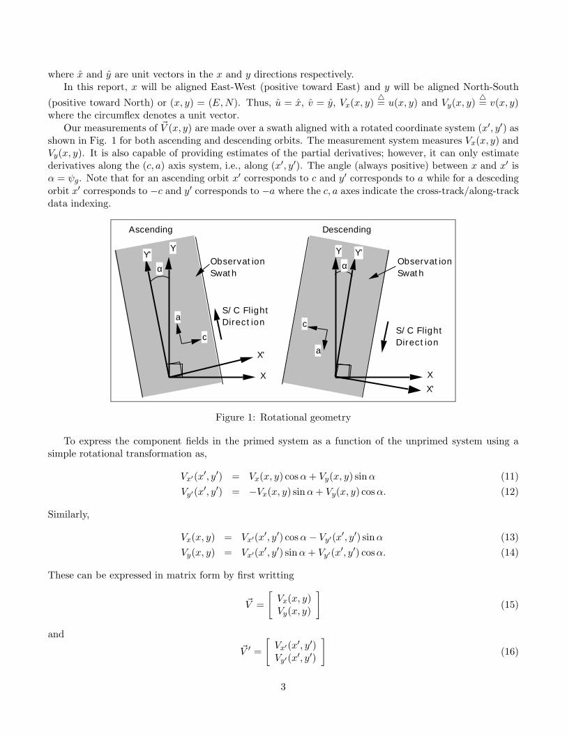
NSCAT defines the relative beam azimuth as degrees CW from North so that for an ascending orbitthe relative azimuth angle for the forward beam on the right side (looking from above in the directionof the flight) is just less than 45◦. ERS-1, on the other hand, defines the relative angle differently. Tocompute the ERS-1 relative azimuth angle stand on the measurement cell facing North. Rotate CW sothat you are facing back along the radar illumination to the spacecraft. Thus, for the right-side forward

6

beam the azimuth angle is somewhat less than 45 + 180◦ = 225 (i.e., ψa = ψ − α + 180◦) for an ascendingswath. So, for a wind from North to South with the antenna at a relative azimuth angle of 0◦ to North(the spacecraft would be exactly North of the measurement cell), the relative radar illumination angle is 0◦

[R. Scott Dunbar, personal communication]. (See Fig. 2.)

α

NorthSpacecraftGround Track

Cell

ϕ

N

ϕa

Subsatellite Point

α

North

Cell

ϕ

ϕa=0°

GeneralCase

Special case Relative Azimuth angle = 0

Figure 2: ERS-1 Relative Azimuth Geometry Examples

4 Vorticity and Divergence

The divergence of ~V (x, y) is defined as,

Div{~V (x, y)} 4=

∂

∂xVx(x, y) +

∂

∂yVy(x, y)

=∂

∂xu +

∂

∂yv. (44)

The vorticity of ~V (x, y) is defined as,

Vor{~V (x, y)} 4= −

∂

∂yVx(x, y) +

∂

∂xVy(x, y)

= −∂

∂yu +

∂

∂xv. (45)

4.1 Taking Partial Derivatives in Mixed Coordinate Systems

Given that the scatterometer samples the wind field in a uniform (x′, y′) grid and we are interested inwind components in the (x, y) = (E, N) coordinate system, several questions arise: 1) Can we computethe partials with respect to the unprimed coordinate system, i.e. with respect to (x, y), from the primed

7

coordinate system? 2) What is the relationship of the curl and diverence computed in the primed systemwith the unprimed system?

We note that the partials can be written as,

∂

∂x=

∂

∂x′∂x′

∂x+

∂

∂y′∂y′

∂x(46)

∂

∂y=

∂

∂y′∂y′

∂y+

∂

∂x′∂x′

∂y. (47)

Since

∂x′

∂x= cosα (48)

∂y′

∂y= cosα (49)

∂y′

∂x= − sinα (50)

∂x′

∂y= sinα, (51)

it follows that

∂

∂x= cosα

∂

∂x′ − sinα∂

∂y′ (52)

∂

∂y= cosα

∂

∂y′ + sinα∂

∂x′ . (53)

Defining

~∂ =

∂

∂x∂

∂y

(54)

and

~∂′ =

∂

∂x′∂

∂y′

(55)

we see that this is a simple rotation,~∂ = T (−α)~∂ ′. (56)

We can reverse the process by noting that,

∂

∂x′ =∂

∂x

∂x

∂x′ +∂

∂y

∂y

∂x′ (57)

∂

∂y′ =∂

∂y

∂y

∂y′ +∂

∂x

∂x

∂y′ . (58)

and

∂x

∂x′ = cos α (59)

8

∂y

∂y′ = cos α (60)

∂y

∂x′ = sinα (61)

∂x

∂y′ = − sinα, (62)

it follows that

∂

∂x′ = cos α∂

∂x+ sinα

∂

∂y(63)

∂

∂y′ = cos α∂

∂y− sinα

∂

∂x. (64)

which, again, is a simple rotation,~∂ ′ = T (α)~∂. (65)

4.2 Divergence and Vorticity in Mixed Coordinate Systems

We now take the divergence of our vector field ~V (dropping the arguments for simplicity), substituting fromprevious results,

Div(x,y){~V } =∂

∂xVx +

∂

∂yVy (66)

=∂

∂x

[Vx′ cosα − Vy′ sinα

]+

∂

∂y

[Vx′ sinα + Vy′ cos α

](67)

= cos α

[∂

∂xVx′ +

∂

∂yVy′

]− sinα

[− ∂

∂yVx′ +

∂

∂xVy′

](68)

= cos αDiv(x,y){~V ′} − sinαVor(x,y){~V ′} (69)

which is a mixed coordinate system result. Making further substitutions,

Div(x,y){~V } = cos α

[∂

∂xVx′ +

∂

∂yVy′

]− sinα

[−

∂

∂yVx′ +

∂

∂xVy′

](70)

= cos α

[cos α

∂

∂x′ Vx′ − sinα∂

∂y′ Vx′ + cos α∂

∂y′ Vy′ + sinα∂

∂x′ Vy′

](71)

− sinα

[− cos α

∂

∂y′ Vx′ − sinα∂

∂x′ Vx′ cos α∂

∂x′Vy′ − sinα∂

∂y′ Vy′

](72)

= cos2 α

[∂

∂x′ Vx′ +∂

∂y′ Vy′

]+ sin2 α

[∂

∂x′ Vx′ +∂

∂y′ Vy′

](73)

=∂

∂x′ Vx′ +∂

∂y′ Vy′ (74)

= Div(x′,y′){~V ′} (75)

which shows that divergence is rotationally invariant.Taking the vorticity of ~V ,

Vor(x,y){~V } = −∂

∂yVx +

∂

∂xVy (76)

9

= − ∂

∂y

[Vx′ cos α − Vy′ sinα

]+

∂

∂x

[Vx′ sinα + Vy′ cosα

](77)

= cos α

[− ∂

∂yVx′ +

∂

∂xVy′

]+ sinα

[∂

∂xVx′ +

∂

∂yVy′

](78)

= cos αVor(x,y){~V ′} + sinαDiv(x,y){~V ′}, (79)

Which is the mixed coordinate system result. Making further substitutions,

Vor(x,y){~V } = cos α

[− ∂

∂yVx′ +

∂

∂xVy′

]+ sinα

[∂

∂xVx′ +

∂

∂yVy′

](80)

= cos α

[− cosα

∂

∂y′ Vx′ − sinα∂

∂x′ Vx′ + cos α∂

∂x′ Vy′ − sinα∂

∂y′ Vy′

](81)

+ sinα

[cosα

∂

∂x′ Vx′ − sinα∂

∂y′ Vx′ + cos α∂

∂y′ Vy′ + sinα∂

∂x′ Vy′

](82)

= cos2 α

[−

∂

∂y′ Vx′ +∂

∂x′ Vy′

]+ sin2 α

[−

∂

∂y′ Vx′ +∂

∂x′ Vy′

](83)

= −∂

∂y′ Vx′ +∂

∂y′ Vx′ (84)

= Vor(x′,y′){~V ′} (85)

which shows that vorticity is rotationally invariant.Defining,

Q(x,y) =

[Div(x,y){~V }Vor(x,y){~V }

](86)

Q′(x,y) =

[Div(x,y){~V ′}Vor(x,y){~V ′}

](87)

Q(x′,y′) =

[Div(x′,y′){~V }Vor(x′,y′){~V }

](88)

Q′(x′,y′) =

[Div(x′,y′){~V ′}Vor(x′,y′){~V ′}

](89)

we can writeQ(x,y) = T (−α)Q′

(x,y). (90)

Thus, the transformation of coordinates results in a rotation of the mixed coordinate divergence andvorticity fields. For the transformation in the other direction,

Div(x′,y′){~V ′} =∂

∂x′ Vx′ +∂

∂y′ Vy′ (91)

=∂

∂x′ [Vx cos α + Vy sinα] +∂

∂y′ [−Vx sinα + Vy cosα] (92)

= cosα

[∂

∂x′ Vx +∂

∂y′ Vy

]+ sinα

[− ∂

∂y′ Vx +∂

∂x′ Vy

](93)

= cosαDiv(x′,y′){~V } + sinαVor(x′,y′){~V } (94)

10

and

Vor(x′,y′){~V ′} = −∂

∂y′ Vx′ +∂

∂x′ Vy′ (95)

= − ∂

∂y′ [Vx cos α + Vy sinα] +∂

∂x′ [−Vx sinα + Vy cos α] (96)

= cosα

[− ∂

∂yVx +

∂

∂xVy′

]− sinα

[∂

∂xVx′ +

∂

∂yVy

](97)

= cosαVor(x′,y′){~V } − sinαDiv(x′,y′){~V } (98)

so thatQ′

(x′,y′) = T (α)Q(x′,y′). (99)

Since the vorticity and divergence fields are rotationally invariant (i.e., their values are not dependenton the coordinate system chosen) we have,

Q(x,y) = Q′(x′,y′) (100)

T (−α)Q′(x,y) = T (α)Q(x′,y′). (101)

A relationship between the mixed coordinate results can be obtained, i.e.,

Q′(x,y) = T−1(−α)T (α)Q(x′,y′) (102)

Q′(x,y) = T (α)T (α)Q(x′,y′) (103)

Q′(x,y) = T 2(α)Q(x′,y′) (104)

Q′(x,y) =

[cos2 α − sin2 α 0

0 cos2 α − sin2 α

]Q(x′,y′). (105)

It follows that

Div(x,y){~V ′} = βDiv(x′,y′){~V } (106)

Vor(x,y){~V ′} = βVor(x′,y′){~V } (107)

whereβ = cos2 α − sin2 α = cos 2α. (108)

5 Estimating the Vorticity and Divergence

Consider a wind field ~Vo specified by a scalar speed S(ci, aj) and direction φo(ci, aj) fields sampled onrectangular grid in the c, a coordinate system where ci = i∆c and aj = j∆a. φo(ci, aj) is the oceanographicconvention angle relative to true North. Then,

u(ci, aj) = S(ci, aj) cos φu(ci, aj) (109)

v(ci, aj) = S(ci, aj) sinφu(ci, aj) (110)

where φu(ci, aj) = 90◦ − φo(ci, aj).

11

A first-order estimate of the partials of u and v with respect to c and a are,

∂

∂cu(c, a) ≈

1∆c

[u(ci, aj) − u(c(i−1), aj)

](111)

∂

∂cv(c, a) ≈ 1

∆c

[v(ci, aj) − v(c(i−1), aj)

](112)

∂

∂au(c, a) ≈

1∆a

[u(ci, aj) − u(ci, a(j−1))

](113)

∂

∂av(c, a) ≈

1∆a

[v(ci, aj) − v(ci, a(j−1))

]. (114)

Noting that y′ is in the same direction of a for ascending orbits we obtain

∂

∂y′ u ≈ 1∆a

[u(ci, aj) − u(ci, a(j−1))

](115)

∂

∂y′ v ≈ 1∆a

[v(ci, aj) − v(ci, a(j−1))

](116)

while for descending orbits we obtain

∂

∂y′ u ≈ − 1∆a

[u(ci, aj) − u(ci, a(j−1))

](117)

∂

∂y′ v ≈ −1

∆a

[v(ci, aj) − v(ci, a(j−1))

]. (118)

Since x′ is in the the same direction as c we obtain the following for ascending orbits

∂

∂x′ u ≈1

∆c

[u(ci, aj) − u(c(i−1), aj)

](119)

∂

∂x′ v ≈ 1∆c

[v(ci, aj) − v(c(i−1), aj)

](120)

and since x′ is in the opposite direction of c

∂

∂x′ u ≈ − 1∆c

[u(ci, aj) − u(c(i−1), aj)

](121)

∂

∂x′ v ≈ −1

∆c

[v(ci, aj) − v(c(i−1), aj)

](122)

for descending orbits. Using the definition of δ in Eq. (22) these equations can be unified,

∂

∂y′ u ≈ δ

∆a

[u(ci, aj) − u(ci, a(j−1))

](123)

∂

∂y′ v ≈ δ

∆a

[v(ci, aj) − v(ci, a(j−1))

](124)

∂

∂x′ u ≈ δ

∆c

[u(ci, aj) − u(c(i−1), aj)

](125)

∂

∂x′ v ≈ δ

∆c

[v(ci, aj) − v(c(i−1), aj)

]. (126)

We can then apply the previous results to obtain the vorticity and divergence in the primed (x′, y′)system,

Div(x′,y′){~V (x, y)} =∂

∂x′ u +∂

∂y′ v (127)

Vor{~V (x, y)} = − ∂

∂y′ u +∂

∂x′ v. (128)

12

which is rotated to obtain the vorticity and divergence in the unprimed (x, y) system,[

Div(x,y){~V }Vor(x,y){~V }

]= T (α)

[Div(x′,y′){~V }Vor(x′,y′){~V }

]. (129)

5.1 Mixed Coordinates

Suppose, however, that we begin with ~Vo = [uo, vo]t where

uo(ci, aj) = S(ci, aj) cos φo(ci, aj) (130)vo(ci, aj) = S(ci, aj) sinφo(ci, aj) (131)

and the partials

∂

∂cuo(c, a) ≈

1∆c

[uo(ci, aj) − uo(c(i−1), aj)

](132)

∂

∂cvo(c, a) ≈ 1

∆c

[vo(ci, aj) − vo(c(i−1), aj)

](133)

∂

∂auo(c, a) ≈

1∆a

[uo(ci, aj) − uo(ci, a(j−1))

](134)

∂

∂avo(c, a) ≈

1∆a

[vo(ci, aj) − vo(ci, a(j−1))

](135)

with the mixed coordinate divergence and curl

Div(c,a){~Vo} =∂

∂cuo(c, a) +

∂

∂avo(c, a) (136)

Vor(c,a){~Vo} = −∂

∂auo(c, a) +

∂

∂cvo(c, a). (137)

These are the equations which have been used to-date in the wind field model.From the geometry of the problem we see that for an ascending orbit

∂

∂x′ =∂

∂c(138)

∂

∂y′ =∂

∂a(139)

and for a descending orbit,

∂

∂x′ = − ∂

∂c(140)

∂

∂y′ = −∂

∂a(141)

can be expressed as

∂

∂x′ = δ∂

∂c(142)

∂

∂y′ = δ∂

∂a. (143)

13

But, since u = vo and v = uo,

∂

∂x′ uo =∂

∂x′ v (144)

∂

∂x′ vo =∂

∂x′ u (145)

∂

∂y′ uo =∂

∂y′ v (146)

∂

∂y′ vo =∂

∂y′ u. (147)

It then follows that

∂

∂x′ u =∂

∂x′ vo = δ∂

∂cvo ≈

δ

∆c

[vo(ci, aj) − vo(c(i−1), aj)

](148)

∂

∂x′ v =∂

∂x′ uo = δ∂

∂cuo ≈ δ

∆c

[uo(ci, aj) − uo(c(i−1), aj)

](149)

∂

∂y′ u =∂

∂y′ vo = δ∂

∂avo ≈ δ

∆a

[vo(ci, aj) − vo(ci, a(j−1))

](150)

∂

∂y′ v =∂

∂y′ uo = δ∂

∂auo ≈ δ

∆a

[uo(ci, aj) − uo(ci, a(j−1))

]. (151)

With this result we can compute the divergence and vorticity of the (u, v) wind in the (x′, y′) coordinatesystem using Eqs. (127) and (128), apply the rotation given in Eq. (129), and determine the consistentdivergence and vorticity of the (u, v) wind in the (x, y) coordinate system.

Examination of the mixed coordinate divergence and vorticity in Eq. (136) reveals,

δDiv(c,a){~Vo} = δ

(∂

∂cuo(c, a) +

∂

∂avo(c, a)

)(152)

=∂

∂x′ uo +∂

∂y′ vo (153)

=∂

∂x′ v +∂

∂y′ u (154)

δVor(c,a){~Vo} = δ

(− ∂

∂auo(c, a) +

∂

∂cvo(c, a)

)(155)

= −∂

∂y′ uo +∂

∂x′ vo (156)

= − ∂

∂y′ v +∂

∂x′ u (157)

As can be seen, there is no simple way to compute the consistent vorticity and divergence from this mixedvorticity and divergence.

6 Wind Field Plotting

Let us now consider the problem of plotting wind vectors for display. This requires transforming thewind vectors from their internal storage convention to a plotting coordinate system (xp, yp). The graphicsdisplay and hardcopy output uses a right-handed (x, y) coordinate system with xp defined postive along thehorizontal axis and yp positive in the vertical direction. Angles are counter-clockwise (CCW) from the xp

14

axis. To display wind vectors we use a subroutine which plots an arrow of specified length (proportionalto the wind speed) with a tail at a specified location and the head at a given CCW angle φp from the xp

axis. By convention, the arrow will display the direction of the atmospheric flow. To enable the display ofthe wind direction when the wind speed is small, frequently a minimum length arrow (corresponding to 0m/s) is used. To this is added a length proportional to the wind speed.

There are two primary display formats used in research at BYU: 1) a rectalinear grid in latitude and lon-gitude (a lat/lon grid) and 2) a rectalinear grid in cross-track and along-track (the mbe grid). Additionally,there are two options for mbe grid plotting.

6.1 Lat/Lon Grid Format

For lat/lon grid plotting the longitude is aligned with xp with positive xp corresponding to East. Latitudeis aligned with yp with positive yp corresponding to North. This results in aligning u (x) with xp and v (y)with yp. As a result

φa = φu = 90◦ − φo = φc − δ′180◦. (158)

This is conceptually the simplest plotting format. The tails of the arrows are located at the lat/lon locationsspecified for each wind vector. This is either computed from the σo measurement data set (the averagelocation of the measurements) or by locating the centers of the wind vector cells on the cross-track/along-track grid and computing the spatial transformation from this coordinate system to lat/lon. A full one-halforbit swath will curve on in this plot format.

6.2 MBE Grid Formats

For plotting in the mbe grid format, we must worry about whether the orbit pass being plotted is ascendingor descending. There are two primary options for mbe grid plotting: 1) plotting all directions with respectto North and 2) plotting all directions with respect to the cross-track/along-track grid. We note that option1 can not be done if the angle of the grid with respect to North, α, is not known. (Note that due to thecurvature of the Earth, α is slightly different for each grid element.)

Figure 3 illustrates the coordinate systems for each option. In both options the along-track coordinateis aligned with xp with positive xp corresponding to increasing along-track distance. Cross-track distanceis aligned with yp with negative yp corresponding to increasing cross-track distance. Land is plotted from amap data set.

6.2.1 Plotting with Respect to MBE Grid

This is the simplest option for mbe grid plotting. In this format option, winds are plotted with respect tothe mbe grid without regard to absolute north. All that is required is that vector directions be consistentwith the (c,a) axes. To do this we let

φp = φc − 90◦ = φu − δ90◦ = φmbe − 90◦. (159)

Land is indicated using land flags in the data set. Grid elements with no measurements may not have landflags even if the grid element is over land.

6.2.2 Plotting with Respect to North

For plotting with respect to North the angle α of the mbe grid with respect to North must be known. Then,

φp = φc − 90◦ = φu − δ90◦ − δα = φmbe − 90◦ − δα. (160)

15

a

c Yp

Xp

N

M

E,X

N,Y

a

cYp

Xp

N

M

E,X

N,Y

φpφpφu

φu

φcφc

φoφo

ASCENDING DESCENDING

With Respect to North

a

cYp

XpN

M

N,Y

a

cYp

XpN

M

N,Y

φpφp

φcφc

ASCENDING DESCENDING

MBE Grid

Figure 3: Plotting geometry

Tails of the wind vector arrows are located at the centers of the cross-track/along track grid elements.Land is indicated using land flags in the data set. Grid elements with no measurements may not have landflags even if the grid element is over land. A spatial transformation must be used to convert latitude andlongitude to cross-track and along-track coordinates which may then be plotted. Latitude/longitude linescurve in this plot format.

16