Distributed Estimation via Iterative Projections with

Application to Power Network Monitoring

Fabio Pasqualetti a, Ruggero Carli b, Francesco Bullo a

aCenter for Control, Dynamical Systems and Computation, University of California, Santa Barbara, USA{fabiopas,bullo}@engineering.ucsb.edu

bDepartement of Information Engineering, University of Padova, Padova, Italycarlirug@dei.unipd.it

Abstract

This work presents a distributed method for control centers to monitor the operating condition of a power network, i.e., toestimate the network state, and to ultimately determine the occurrence of threatening situations. State estimation has beenrecognized to be a fundamental task for network control centers to ensure correct and safe functionalities of power grids.We consider (static) state estimation problems, in which the state vector consists of the voltage magnitude and angle atall network buses. We consider the state to be linearly related to network measurements, which include power flows, currentinjections, and voltages phasors at some buses. We admit the presence of several cooperating control centers, and we design twodistributed methods for them to compute the minimum variance estimate of the state given the network measurements. Thetwo distributed methods rely on different modes of cooperation among control centers: in the first method an incremental modeof cooperation is used, whereas, in the second method, a diffusive interaction is implemented. Our procedures, which requireeach control center to know only the measurements and structure of a subpart of the whole network, are computationallyefficient and scalable with respect to the network dimension, provided that the number of control centers also increases withthe network cardinality. Additionally, a finite-memory approximation of our diffusive algorithm is proposed, and its accuracyis characterized. Finally, our estimation methods are exploited to develop a distributed algorithm to detect corrupted dataamong the network measurements.

1 Introduction

Large-scale complex systems, such as, for instance, the electrical power grid and the telecommunication system,are receiving increasing attention from researchers in different fields. The wide spatial distribution and the highdimensionality of these systems preclude the use of centralized solutions to tackle classical estimation, control,and fault detection problems, and they require, instead, the development of new decentralized techniques. Onepossibility to overcome these issues is to geographically deploy some monitors in the network, each one responsiblefor a different subpart of the whole system. Local estimation and control schemes can successively be used, togetherwith an information exchange mechanism to recover the performance of a centralized scheme.

1.1 Control centers, state estimation and cyber security in power networks

Power systems are operated by system operators from the area control center. The main goal of the system operatoris to maintain the network in a secure operating condition, in which all the loads are supplied power by the generatorswithout violating the operational limits on the transmission lines. In order to accomplish this goal, at a given point

? This material is based in part upon work supported by ICB ARO grant W911NF-09-D-0001 and NSF grant CNS-0834446,and in part upon the EC Contract IST 224428 ”CHAT”.

Email addresses: fabiopas@engineering.ucsb.edu (Fabio Pasqualetti), carlirug@dei.unipd.it (Ruggero Carli),bullo@engineering.ucsb.edu (Francesco Bullo).

Preprint submitted to Automatica 11 July 2011

RTU RTU RTU RTU

LAN

SCADA

CONTROL

CENTER { • Estimation

• Control

• Optimization

. . .

Monitored devices

(a)

� �

�

�

� �

�

�

��

��

��

��

��

���

��

��

��

��

��

��

��

��

��

��

��

��

��

��

��� ��

��

��

������

��

��

��

��

��

��

��

�� �� ��

��

��

��

����

��

��

��

��

��

�� �� ����

����

��

��

��

��

��

��

��

��

��

��

���

��

��

��

��

��

��

��

��

��� ��

��

��

��

��

��

��

����

��

��

��

�� ��

����

��

��

����

��

��

��

��

���

������

���

��� ���

���

���

���

���

���

���

���

G

G

G

G

G G

G

G

GG

G

GG

G

G

G

G G

G

G

G

G

G G

G G

G

G G

G

G

G

G

G G G G G

G

G

�

G

G

G

G

G

G

G

G

G

G

G

G

G

G

2QH�OLQH�'LDJUDP�RI�,(((�����EXV�7HVW�6\VWHP

,,7�3RZHU�*URXS������

6\VWHP�'HVFULSWLRQ�

����EXVHV����EUDQFKHV���ORDG�VLGHV���WKHUPDO�XQLWV

(b)

Fig. 1. In Fig. 1(a), remote terminal units (RTU) transmit their measurements to a SCADA terminal via a LAN network.The data is then sent to a Control Center to implement network estimation, control, and optimization procedures. Fig. 1(b)shows the diagram of the IEEE 118 bus system (courtesy of the IIT Power Group). The network has 118 buses, 186 branches,99 loads, and 54 generators.

in time, the network model and the phasor voltages at every system bus need to be determined, and preventiveactions have to be taken if the system is found in an insecure state. For the determination of the operating state,remote terminal units and measuring devices are deployed in the network to gather measurements. These devicesare then connected via a local area network to a SCADA (Supervisory Control and Data Acquisition) terminal,which supports the communication of the collected measurements to a control center. At the control center, themeasurement data is used for control and optimization functions, such as contingency analysis, automatic generationcontrol, load forecasting, optimal power flow computation, and reactive power dispatch [1]. A diagram representingthe interconnections between remote terminal units and the control center is reported in Fig. 1(a). Various sourcesof uncertainties, e.g., measurement and communication noise, lead to inaccuracies in the received data, which mayaffect the performance of the control and optimization algorithms, and, ultimately, the stability of the power plant.This concern was first recognized and addressed in [27, 28, 29] by introducing the idea of (static) state estimationin power systems.

Power network state estimators are broadly used to obtain an optimal estimate from redundant noisy measure-ments, and to estimate the state of a network branch which, for economical or computational reasons, is not directlymonitored. For the power system state estimation problem, several centralized and parallel solutions have been de-veloped in the last decades, e.g., see [19, 8, 30]. Being an online function, computational issues, storage requirements,and numerical robustness of the solution algorithm need to be taken into account. Within this regard, distributedalgorithms based on network partitioning techniques are to be preferred over centralized ones. Moreover, even indecentralized setting, the work in [20] on the blackout of August 2003 suggests that an estimation of the entirenetwork is essential to prevent networks damages. In other words, the whole state vector should be estimated byand available to every unit. The references [34, 12] explore the idea of using a global control center to coordinateestimates obtained locally by several local control centers. In this work, we improve upon these prior results byproposing a fully decentralized and distributed estimation algorithm, which, by only assuming local knowledge ofthe network structure by the local control centers, allows them to obtain in finite time an optimal estimate of thenetwork state. Being the computation distributed among the control centers, our procedure appears scalable againstthe power network dimension, and, furthermore, numerically reliable and accurate.

A second focus of this paper is false data detection and cyber attacks in power systems. Because of the increasingreliance of modern power systems on communication networks, the possibility of cyber attacks is a real threat[18]. One possibility for the attacker is to corrupt the data coming from the measuring units and directed to thecontrol center, in order to introduce arbitrary errors in the estimated state, and, consequently, to compromise theperformance of control and optimization algorithms [14]. This important type of attack is often referred in thepower systems literature to as false data injection attack. Recently, the authors of [33] show that a false datainjection attack, in addition to destabilizing the grid, may also lead to fluctuations in the electricity market, causing

2

significant economical losses. The presence of false data is classically checked by analyzing the statistical propertiesof the estimation residual z −Hx, where z is the measurements vector, x is a state estimate, and H is the state tomeasurements matrix. For an attack to be successful, the residual needs to remain within a certain confidence level.Accordingly, one approach to circumvent false data injection attacks is to increase the number of measurements soas to obtain a more accurate confidence bound. Clearly, by increasing the number of measurements, the data to betransmitted to the control center increases, and the dimension of the estimation problem grows. By means of ourestimation method, we address this dimensionality problem by distributing the false data detection problem amongseveral control centers.

1.2 Related work on distributed estimation and projection methods

Starting from the eighties, the problem of distributed estimation has attracted intense attention from the scientificcommunity, generating along the years a very rich literature. More recently, because of the advent of highly integratedand low-cost wireless devices as key components of large autonomous networks, the interest for this classical topic hasbeen renewed. For a wireless sensor network, novel applications requiring efficient distributed estimation proceduresinclude, for instance, environment monitoring, surveillance, localization, and target tracking. Considerable effort hasbeen devoted to the development of distributed and adaptive filtering schemes, which generalize the notion of adaptiveestimation to a setup involving networked sensing and processing devices [4]. In this context, relevant methods includeincremental Least Mean-Square [15], incremental Recursive Least-Square [24], Diffusive Least Mean-Square [24], andDiffusive Recursive Least-Square[4]. Diffusion Kalman filtering and smoothing algorithms are proposed, for instance,in [3, 5], and consensus based techniques in [25, 26]. We remark that the strategies proposed in the aforementionedreferences could be adapted for the solution of the power network static estimation problem. Their assumptions,however, appear to be not well suited in our context for the following reasons. First, the convergence of the aboveestimation algorithms is only asymptotic, and it depends upon the communication topology. As a matter of fact, formany communication topologies, such as Cayley graphs and random geometric graphs, the convergence rate is veryslow and scales badly with the network dimension. Such slow convergence rate is clearly undesirable because a delayedstate estimation could lead the power plant to instability. Second, approaches based on Kalman filtering require theknowledge of the global state and observation model by all the components of the network, and they violate thereforeour assumptions. Third and finally, the application of these methods to the detection of cyber attacks, which is alsoour goal, is not straightforward, especially when detection guarantees are required. An exception is constituted by[31], where a estimation technique based on local Kalman filters and a consensus strategy is developed. This lattermethod, however, besides exhibiting asymptotic convergence, does not offer guarantees on the final estimation error.

Our estimation technique belongs to the family of Kaczmarz (row-projection) methods for the solution of a linearsystem of equations. See [13, 11, 32, 6] for a detailed discussion. Differently from the existing row-action methods,our algorithms exhibit finite time convergence towards the exact solution, and they can be used to compute anyweighted least squares solution to a system of linear equations.

1.3 Our contributions

The contributions of this work are threefold. First, we adopt the static state network estimation model, in which thestate vector is linearly related to the network measurements. We develop two methods for a group of interconnectedcontrol centers to compute an optimal estimate of the system state via distributed computation. Our first estimationalgorithm assumes an incremental mode of cooperation among the control centers, while our second estimationalgorithm is based upon a diffusive strategy. Both methods are shown to converge in a finite number of iterations,and to require only local information for their implementation. Differently than [23], our estimation proceduresassume neither the measurement error covariance nor the measurements matrix to be diagonal. Furthermore, ouralgorithms are advantageous from a communication perspective, since they reduce the distance between remoteterminal units and the associated control center, and from a computational perspective, since they distribute themeasurements to be processed among the control centers. Second, as a minor contribution, we describe a finite-timealgorithm to detect via distributed computation if the measurements have been corrupted by a malignant agent. Ourdetection method is based upon our state estimation technique, and it inherits its convergence properties. Notice that,since we assume the measurements to be corrupted by noise, the possibility exists for an attacker to compromise thenetwork measurements while remaining undetected (by injecting for instance a vector with the same noise statistics).With respect to this limitation, we characterize the class of corrupted vectors that are guaranteed to be detectedby our procedure, and we show optimality with respect to a centralized detection algorithm. Third, we study thescalability of our methods in networks of increasing dimension, and we derive a finite-memory approximation of ourdiffusive estimation strategy. For this approximation procedure we show that, under a reasonable set of assumptions

3

and independent of the network dimension, each control center is able to recover a good approximation of the stateof a certain subnetwork through little computation. Moreover, we provide bounds on the approximation error foreach subnetwork. Finally, we illustrate the effectiveness of our procedures on the IEEE 118 bus system.

The rest of the paper is organized as follows. In Section 2 we introduce the problem under consideration, and wedescribe the mathematical setup. Section 3 contains our main results on the state estimation and on the detectionproblem, as well as our algorithms. Section 4 describes our approximated state estimation algorithm. In Section 5 westudy the IEEE 118 bus system, and we present some simulation results. Finally, Section 6 contains our conclusion.

2 Problem setup and preliminary notions

For a power network, an example of which is reported in Fig. 1(b), the state at a certain instant of time consistsof the voltage angles and magnitudes at all the system buses. The (static) state estimation problem introducedin the seminal work by Schweppe [27] refers to the procedure of estimating the state of a power network given aset of measurements of the network variables, such as, for instance, voltages, currents, and power flows along thetransmission lines. To be more precise, let x ∈ Rn and z ∈ Rp be, respectively, the state and measurements vector.Then, the vectors x and z are related by the relation

z = h(x) + η, (1)

where h(·) is a nonlinear measurement function, and where η, which is traditionally assumed to be a zero meanrandom vector satisfying E[ηηT] = Ση = ΣT

η > 0, is the noise measurement. An optimal estimate of the network statecoincides with the most likely vector x that solves equation (1). It should be observed that, instead of by solving theabove estimation problem, the network state could be obtained by measuring directly the voltage phasors by meansof phasor measurement devices. 1 Such an approach, however, would be economically expensive, since it requires todeploy a phasor measurement device at each network bus, and it would be very vulnerable to communication failures[1]. In this work, we adopt the approximated estimation model presented in [28], which follows from the linearizationaround the origin of equation (1). Specifically,

z = Hx + v, (2)

where H ∈ Rp×n and where v, the noise measurement, is such that E[v] = 0 andE[vvT] = Σ = ΣT > 0. Observethat, because of the interconnection structure of a power network, the measurement matrix H is usually sparse. LetKer(H) denote the null space defined by the matrix H. For the equation (2), without affecting generality, assumeKer(H) = {0}, and recall from [17] that the vector

xwls = (HTΣ−1H)−1HTΣ−1z (3)

minimizes the weighted variance of the estimation error, i.e., xwls = arg minx(z −Hx)TΣ−1(z −Hx).

The centralized computation of the minimum variance estimate to (2) assumes the complete knowledge of the matricesH and Σ, and it requires the inversion of the matrix HTΣ−1H. For a large power network, such computation imposesa limitation on the dimension of the matrix H, and hence on the number of measurements that can be efficientlyprocessed to obtain a real-time state estimate. Since the performance of network control and optimization algorithmsdepend upon the precision of the state estimate, a limitation on the network measurements constitutes a bottlenecktoward the development of a more efficient power grid. A possible solution to address this complexity problem isto distribute the computation of xwls among geographically deployed control centers (monitors), in a way that eachmonitor is responsible for a subpart of the whole network. To be more precise, let the matrices H and Σ, and the

1 Phasor measurement units are devices that synchronize by using GPS signals, and that allow for a direct measurement ofvoltage and current phasors.

4

vector z be partitioned as 2

H =

H1

H2

...

Hm

, Σ =

Σ1

Σ2

...

Σm

, z =

z1

z2

...

zm

, (4)

where, for i ∈ {1, . . . ,m}, mi ∈ N, Hi ∈ Rmi×n, Σi ∈ Rmi×p, zi ∈ Rmi , and∑m

i=1 mi = p. Let G = (V, E) be aconnected graph in which each vertex i ∈ V = {1, . . . ,m} denotes a monitor, and E ∈ V × V denotes the set ofmonitors interconnections. For i ∈ {1, . . . ,m}, assume that monitor i knows the matrices Hi, Σi, and the vector zi.Moreover, assume that two neighboring monitors are allowed to cooperate by exchanging information. Notice that, ifthe full matrices H and Σ are nowhere available, and if they cannot be used for the computation of xwls, then, withno cooperation among the monitors, the vector xwls cannot be computed by any of the monitor. Hence we considerthe following problem.

Problem 1 (Distributed state estimation) Design an algorithm for the monitors to compute the minimum vari-ance estimate of the network state via distributed computation.

We now introduce the second problem addressed in this work. Given the distributed nature of a power system andthe increasing reliance on local area networks to transmit data to a control center, there exists the possibility for anattacker to compromise the network functionality by corrupting the measurements vector. When a malignant agentcorrupts some of the measurements, the state to measurements relation becomes

z = Hx + v + w,

where the vector w ∈ Rp is chosen by the attacker, and, therefore, it is unknown and unmeasurable by any of themonitoring stations. We refer to the vector w to as false data. From the above equation, it should be observed thatthere exist vectors w that cannot be detected through the measurements z. For instance, if the false data vector isintentionally chosen such that w ∈ Im(H), then the attack cannot be detected through the measurements z. Indeed,denoting with † the pseudoinverse operation, the vector x + H†w is a valid network state. In this work, we assumethat the vector w is detectable from the measurements z, and we consider the following problem.

Problem 2 (Distributed detection) Design an algorithm for the monitors to detect the presence of false data inthe measurements via distributed computation.

As it will be clear in the sequel, the complexity of our methods depends upon the dimension of the state, as wellas the number of monitors. In particular, few monitors should be used in the absence of severe computation andcommunication contraints, while many monitors are preferred otherwise. We believe that a suitable choice of thenumber of monitors depends upon the specific scenario, and it is not further discussed in this work.

Remark 1 (Generality of our methods) In this paper we focus on the state estimation and the false data detec-tion problem for power systems, because this field of research is currently receiving sensible attention from differentcommunities. The methods described in the following sections, however, are general, and they have applicabilitybeyond the power network scenario. For instance, our procedures can be used for state estimation and false datadetection in dynamical system, as described in [21] for the case of sensors networks.

3 Optimal state estimation and false data detection via distributed computation

The objective of this section is the design of distributed methods to compute an optimal state estimate frommeasurements. With respect to a centralized method, in which a powerful central processor is in charge of processing

2 In most application the error covariance matrix is assumed to be diagonal, so that each submatrix Σi is very sparse.However, we do not impose any particular structure on the error covariance matrix.

5

Algorithm 1 Incremental minimum norm solution (i-th monitor)Input: Hi, zi;Require: [zT

1 . . . zTm]T ∈ Im([HT

1 . . . HTm]T);

if i = 1 thenx0 := 0, K0 := In;

elsereceive xi−1 and Ki−1 from monitor i− 1;

end ifxi := xi−1 + Ki−1(HiKi−1)†(zi −Hixi−1);Ki := Basis(Ki−1 Ker(HiKi−1));if i < m then

transmit xi and Ki to monitor i + 1;else

return xm;end if

all the data, our procedures require the computing units to have access to only a subset of the measurements, andare shown to reduce significantly the computational burden. In addition to being convenient for the implementation,our methods are also optimal, in the sense that they maintain the same estimation accuracy of a centralized method.

For a distributed method to be implemented, the interaction structure among the computing units needs to bedefined. Here we consider two modes of cooperations among the computing units, and, namely, the incremental andthe diffusive interaction. In an incremental mode of cooperation, information flows in a sequential manner from onenode to the adjacent one. This setting, which usually requires the least amount of communications [22], induces acyclic interaction graph among the processors. In a diffusive strategy, instead, each node exchanges information withall (or a subset of) its neighbors as defined by an interaction graph. In this case, the amount of communication andcomputation is higher than in the incremental case, but each node possesses a good estimate before the terminationof the algorithm, since it improves its estimate at each communication round. This section is divided into three parts.In Section 3.2, we first develop a distributed incremental method to compute the minimum norm solution to a setof linear equations, and then exploit such method to solve a minimum variance estimation problem. In Section 3.3we derive a diffusive strategy which is amenable to asynchronous implementation. Finally, in Section 3.4 we proposea distributed algorithm for the detection of false data among the measurements. Our detection procedure requiresthe computation of the minimum variance state estimate, for which either the incremental or the diffusive strategycan be used.

3.1 Incremental solution to a set of linear equations

We start by introducing a distributed incremental procedure to compute the minimum norm solution to a set oflinear equations. This procedure constitutes the key ingredient of the incremental method we later propose to solvethe minimum variance estimation problem. Let H ∈ Rp×m, and let z ∈ Im(H), where Im(H) denotes the range spacespanned by the matrix H. Consider the system of linear equations z = Hx, and recall that the unique minimumnorm solution to z = Hx coincides with the vector x such that z = Hx and ‖x‖2 is minimum. It can be shownthat ‖x‖2 being minimum corresponds to x being orthogonal to the null space Ker(H) of H [17]. Let H and z bepartitioned in m blocks as in (4), and let G = (V, E) be a directed graph such that V = {1, . . . ,m} corresponds to theset of monitors, and, denoting with (i, j) the directed edge from j to i, E = {(i + 1, i) : i = 1, . . . ,m− 1} ∪ {(1,m)}.Our incremental procedure to compute the minimum norm solution to z = Hx is in Algorithm 1, where, given asubspace V, we write Basis(V) to denote any full rank matrix whose columns span the subspace V. We now proceedwith the analysis of the convergence properties of the Incremental minimum norm solution algorithm.

Theorem 3.1 (Convergence of Algorithm 1) Let z = Hx, where H and z are partitioned in m row-blocks as in (4).In Algorithm 1, the m-th monitor returns the vector x such that z = Hx and x ⊥ Ker(H).

PROOF. See Section 6.1.

It should be observed that the dimension of Ki decreases, in general, when the index i increases. In particular,Km = {0} and K1 = Ker(H1). To reduce the computational burden of the algorithm, monitor i could transmit the

6

smallest among Basis(Ki−1 Ker(HiKi−1)) and Basis(Ki−1 Ker(HiKi−1)⊥), together with a packet containing thetype of the transmitted basis.

Remark 2 (Computational complexity of Algorithm 1) In Algorithm 1, the main operation to be performedby the i-th agent is a singular value decomposition (SVD). 3 Indeed, since the range space and the null space of amatrix can be obtained through its SVD, both the matrices (HiKi−1)† and Basis(Ki−1 Ker(HiKi−1)) can be recoveredfrom the SVD of HiKi−1. Let H ∈ Rm×n, m > n, and assume the presence of dm/ke monitors, 1 ≤ k ≤ m. Recallthat, for a matrix M ∈ Rk×p, the singular value decomposition can be performed with complexity O(min{kp2, k2p})[10]. Hence, the computational complexity of computing a minimum norm solution to the system z = Hx is O(mn2).In Table 1 we report the computational complexity of Algorithm 1 as a function of the size k.Table 1Computational complexity of Algorithm 1.

Block size I-th complexity Total complexity Communications

k ≤ n O(k2n) O(mkn) dm/ke − 1

k > n O(kn2) O(mn2) dm/ke − 1

The following observations are in order. First, if k ≤ n, then the computational complexity sustained by the i-thmonitor is much smaller than the complexity of a centralized implementation, i.e., O(k2n) � O(mn2). Second, thecomplexity of the entire algorithm is optimal, since, in the worst case, it maintains the computational complexity ofa centralized solution, i.e., O(mkn) ≤ O(mn2). Third and finally, a compromise exists between the blocks size k andthe number of communications needed to terminate Algorithm 1. In particular, if k = m, then no communication isneeded, while, if k = 1, then m− 1 communication rounds are necessary to terminate the estimation algorithm. 4

3.2 Incremental state estimation via distributed computation

We now focus on the computation of the weighted least squares solution to a set of linear equations. Let v be anunknown and unmeasurable random vector, with E(v) = 0 and E(vvT) = Σ = ΣT > 0. Consider the system ofequations

z = Hx + v, (5)

and assume Ker(H) = 0. Notice that, because of the noise vector v, we generally have z 6∈ Im(H), so that Algorithm1 cannot be directly employed to compute the vector xwls defined in (3). It is possible, however, to recast the aboveweighted least squares estimation problem to be solvable with Algorithm 1. Note that, because the matrix Σ issymmetric and positive definite, there exists 5 a full row rank matrix B such that Σ = BBT. Then, equation (5) canbe rewritten as

z =[

H εB] [

x

v

], (6)

where ε ∈ R>0, E[v] = 0 and E[vvT] = ε−2I. Observe that, because B has full row rank, the system (6) isunderdetermined, i.e., z ∈ Im([H εB]) and Ker([H εB]) 6= 0. Let[

x(ε)ˆv

]=

[H εB

]†z. (7)

The following theorem characterizes the relation between the minimum variance estimation xwls and x(ε).

3 The matrix H is usually very sparse, since it reflects the network interconnection structure. Efficient SVD algorithms forvery large sparse matrices are being developed (cf. SVDPACK ).4 Additional m − 1 communication rounds are needed to transmit the estimation to every other monitor.5 Choose for instance B = WΛ1/2, where W is a basis of eigenvectors of Σ and Λ is the corresponding diagonal matrix of theeigenvalues.

7

Theorem 3.2 (Convergence with ε) Consider the system of linear equations z = Hx + v. Let E(v) = 0 andE(vvT) = Σ = BBT > 0 for a full row rank matrix B. Let

C = ε(I −HH†)B, E = I − C†C, D = εE[I + ε2EBT(HHT)†BE]−1BT(HHT)†(I − εBC†).

Then

[H εB

]†=

[H† − εH†B(C† + D)

C† + D

];

and

limε→0+

H† − εH†B(C† + D) = (HTΣ−1H)−1HTΣ−1.

PROOF. See Section 6.2.

Throughout the paper, let x(ε) be the vector defined in (7), and notice that Theorem 3.2 implies that

xwls = limε→0+

x(ε).

Remark 3 (Incremental state estimation) For the system of equations z = Hx + v, let BBT be the covariancematrix of the noise vector v, and let

H =

H1

H2

...

Hm

, B =

B1

B2

...

Bm

, z =

z1

z2

...

zm

, (8)

where mi ∈ N, Hi ∈ Rmi×n, Bi ∈ Rmi×p, and zi ∈ Rmi . For ε > 0, the estimate x(ε) of the weighted least squaressolution to z = Hx + v can be computed by means of Algorithm 1 with input [Hi εBi] and zi.

Observe now that the estimate x(ε) coincides with xwls only in the limit for ε → 0+. When the parameter ε is fixed,the estimate x(ε) differs from the minimum variance estimate xwls. We next characterize the approximation errorxwls − x(ε).

Corollary 3.1 (Approximation error) Consider the system z = Hx + v, and let E[vvT] = BBT for a full row rankmatrix B. Then

xwls − x(ε) = εH†BDz,

where D is as in Theorem 3.2.

PROOF. With the same notation as in the proof of Theorem 3.2, for every value of ε > 0, the difference xwls− x(ε)equals

((HTΣ−1H)−1HTΣ−1 −H† + εH†B(C† + D)

)z. Since (HTΣ−1H)−1HTΣ−1 −H† + εH†BC† = 0 for every

ε > 0, it follows xwls − x(ε) = εH†BDz.

Therefore, for the solution of system (5) by means of Algorithm 1, the parameter ε is chosen according to Corollary3.1 to meet a desired estimation accuracy. It should be observed that, even if the entire matrix H needs to be known

8

for the computation of the exact parameter ε, the advantages of our estimation technique are preserved. Indeed, ifthe matrix H is unknown and an upper bound for ‖H†BDz‖ is known, then a value for ε can still be computed thatguarantees the desired estimation accuracy. On the other hand, even if H is entirely known, it may be inefficientto use H to perform a centralized state estimation over time. Instead, the parameter ε needs to be computed onlyonce. To conclude this section, we characterize the estimation residual z −Hx. This quantity plays an importantrole for the synthesis of a distributed false data detection algorithm.

Corollary 3.2 (Estimation residual) Consider the system z = Hx + v, and let E[vvT] = Σ = ΣT > 0. Then 6

limε→0+

‖z −Hx(ε)‖ ≤ ‖(I −HW )‖‖v‖,

where W = (HTΣ−1H)−1HTΣ−1.

PROOF. By virtue of Theorem 3.2 we have limε→0+ x(ε) = xwls = (HTΣ−1H)−1HTΣ−1z = Wz. Observe thatHWH = H, and recall that z = Hx + v. For any matrix norm, we have

‖z −Hxwls‖ = ‖z −HWz‖ = ‖(I −HW )(Hx + v)‖ = ‖Hx−Hx + (I −HW )v‖ ≤ ‖(I −HW )‖‖v‖,

and the theorem follows.

3.3 Diffusive state estimation via distributed computation

The implementation of the incremental state estimation algorithm described in Section 3.2 requires a certain degreeof coordination among the control centers. For instance, an ordering of the monitors is necessary, such that the i-thmonitor transmits its estimate to the (i + 1)-th monitor. This requirement imposes a constraint on the monitorsinterconnection structure, which may be undesirable, and, potentially, less robust to link failures. In this section, weovercome this limitation by presenting a diffusive implementation of Algorithm 1, which only requires the monitorsinterconnection structure to be connected. 7 To be more precise, let V = {1, . . . ,m} be the set of monitors, andlet G = (V,E) be the undirected graph describing the monitors interconnection structure, where E ⊆ V × V , and(i, j) ∈ E if and only if the monitors i and j are connected. The neighbor set of node i is defined as Ni = {j ∈ V :(i, j) ∈ E}. We assume that G is connected, and we let the distance between two vertices be the minimum number ofedges in a path connecting them. Finally, the diameter of a graph G, in short diam(G), equals the greatest distancebetween any pair of vertices. Our diffusive procedure is described in Algorithm 2, where the matrices Hi and εBi

are as defined in equation (8). During the h-th iteration of the algorithm, monitor i, with i ∈ {1, . . . , N}, performsthe following three actions in order:

(i) transmits its current estimates xi and Ki to all its neighbors;(ii) receives the estimates xj from neighbors Ni; and(iii) updates xi and Ki as in the for loop of Algorithm 2.

We next show the convergence of Algorithm 2 to the minimum variance estimate.

Theorem 3.3 (Convergence of Algorithm 2) Consider the system of linear equations z = Hx+v, where E[v] =0 and E[vvT] = BBT. Let H, B and z be partitioned as in (8), and let ε > 0. Let the monitors communication graphbe connected, let d be its diameter, and let the monitors execute the Diffusive state estimation algorithm. Then, eachmonitor computes the estimate x(ε) of x in d steps.

PROOF. Let xi be the estimate of the monitor i, and let Ki be such that x − xi ∈ Im(Ki), where x denotes thenetwork state, and xi ⊥ Im(Ki). Notice that zi = [Hi εBi]xi, where zi it the i-th measurements vector. Let i and j

6 Given a vector v and a matrix H, we denote by ‖v‖ any vector norm, and by ‖H‖ the corresponding induced matrix norm.7 An undirected graph is said to be connected if there exists a path between any two vertices [9].

9

Algorithm 2 Diffusive state estimation (i-th monitor)Input: Hi, εBi, zi;

xi := [Hi εBi]†zi;Ki := Basis(Ker([Hi εBi]));while Ki 6= 0 do

for j ∈ Ni doreceive xj and Kj ;xi := xi + [Ki 0][−Ki Kj ]†(xi − xj);Ki := Basis(Im(Ki) ∩ Im(Kj));

end fortransmit xi and Ki;

end while

be two neighboring monitors. Notice that there exist vectors vi and vj such that xi +Kivi = xj +Kjvj . In particular,those vectors can be chosen as [

vi

vj

]= [−Ki Kj ]†(xi − xj).

It follows that the vector

x+i = xi + [Ki 0][−Ki Kj ]†(xi − xj)

is such that zi = [Hi εBi]x+i and zj = [Hj εBj ]x+

i . Moreover we have x+i ⊥ (Im(Ki) ∩ Im(Kj)). Indeed, notice that[

vi

vj

]⊥ Ker([−Ki Kj ]) ⊇

{[wi

wj

]: Kiwi = Kjwj

}.

We now show that Kivi ⊥ Im(Kj). By contradiction, if Kivi 6⊥ Im(Kj), then vi = vi + vi, with Kivi ⊥ Im(Kj)and Kivi ∈ Im(Kj). Let vj = K†

j Kivi, and vj = vj − vj . Then, [vTi vT

j ]T ∈ Ker([−Ki Kj ]), and hence [vTi vT

j ]T 6⊥Ker([−Ki Kj ]), which contradicts the hypothesis. We conclude that [Ki 0][−Ki Kj ]†(xi − xj) ⊥ Im(Kj), and,since xi ⊥ Im(Ki), it follows x+

i ⊥ (Im(Ki) ∩ Im(Kj)). The theorem follows from the fact that after a number ofsteps equal to the diameter of the monitors communication graph, each vector xi verifies all the measurements, andxi ⊥ Im(K1) ∩ · · · ∩ Im(Km).

As a consequence of Theorem 3.2, in the limit for ε to zero, Algorithm 2 returns the minimum variance estimateof the state vector, being therefore the diffusive counterpart of Algorithm 1. A detailed comparison between incre-mental and diffusive methods is beyond the purpose of this work, and we refer the interested reader to [15, 16] andthe references therein for a thorough discussion. Here we only underline some key differences. While Algorithm 1requires less operations, being therefore computationally more efficient, Algorithm 2 does not constraint the monitorscommunication graph. Additionally, Algorithm 2 can be implemented adopting general asynchronous communica-tion protocols. For instance, consider the Asynchronous (diffusive) state estimation algorithm, where, at any giveninstant of time in N, at most one monitor, say j, sends its current estimates to its neighbors, and where, for i ∈ Nj ,monitor i performs the following operations:

(i) xi := xi + [Ki 0][−Ki Kj ]†(xi − xj),(ii) Ki := Basis(Im(Ki) ∩ Im(Kj)).

Corollary 3.3 (Asynchronous estimation) Consider the system of linear equations z = Hx+ v, where E[v] = 0and E[vvT] = BBT. Let H, B and z be partitioned as in (8), and let ε > 0. Let the monitors communication graph beconnected, let d be its diameter, and let the monitors execute the Asynchronous (diffusive) state estimation algorithm.Assume that there exists a duration T ∈ N such that, within each time interval of duration T , each monitor transmitsits current estimates to its neighbors. Then, each monitor computes the estimate x(ε) of x within time dT .

10

Algorithm 3 False data detection (i-th monitor)Input: Hi, εBi, Γ;

while True docollect measurements zi(t);estimate network state x(t) via Algorithm 1 or 2if ‖zi(t)−Hix(t)‖∞ > Γ then

return False data detected;end if

end while

PROOF. The proof follows from the following two facts. First, the intersection of subspaces is a commutativeoperation. Second, since each monitor performs a data transmission within any time interval of length T , it followsthat, at time dT , the information related to one monitor has propagated through the network to every other monitor.

3.4 Detection of false data via distributed computation

In the previous sections we have shown how to compute an optimal state estimate via distributed computation. Arather straightforward application of the proposed state estimation technique is the detection of false data amongthe measurements. When the measurements are corrupted, the state to measurements relation becomes

z = Hx + v + w,

where w is the false data vector. As a consequence of Corollary 3.2, the vector w is detectable if it affects significantlythe estimation residual, i.e., if limε→0 ‖z −Hx(ε)‖ > Γ, where the threshold Γ depends upon the magnitude of thenoise v. Notice that, because false data can be injected at any time by a malignant agent, the detection algorithmneeds to be executed over time by the control centers. Let z(t) be the measurements vector at a given time instantt, and let E[z(t1)zT(t2)] = 0 for all t1 6= t2. Based on this considerations, our distributed detection procedure is inAlgorithm 3, where the matrices Hi and εBi are as defined in equation (8), and Γ is a predefined threshold.

In Algorithm 3, the value of the threshold Γ determines the false alarm and the misdetection rate. Clearly, ifΓ ≥ ‖(I−HW )‖‖v(t)‖ and ε is sufficiently small, then no false alarm is triggered, at the expenses of the misdetectionrate. By decreasing the value of Γ the sensitivity to failures increases together with the false alarm rate. Notice that, ifthe magnitude of the noise signals is bounded by γ, then a reasonable choice of the threshold is Γ = γ‖(I−HW )‖∞,where the use of the infinity norm in Algorithm 3 is also convenient for the implementation. Indeed, since thecondition ‖z(t)−Hx(t)‖∞ > Γ is equivalent to ‖zi(t)−Hix(t)‖∞ > Γ for some monitor i, the presence of false datacan be independently checked by each monitor without further computation. Notice that an eventual alarm messageneeds to be propagated to all other control centers.

Remark 4 (Statistical detection) A different strategy for the detection of false data relies on statistical tech-niques, e.g., see [1]. In the interest of brevity, we do not consider these methods, and we only remark that, once theestimation residual has been computed by each monitor, the implementation of a (distributed) statistical procedure,such as, for instance, the (distributed) χ2-Test, is a straightforward task.

4 A finite-memory estimation technique

The procedure described in Algorithm 1 allows each agent to compute an optimal estimate of the whole networkstate in finite time. In this section, we allow each agent to handle only local, i.e., of small dimension, vectors, andwe develop a procedure to recover an estimate of only a certain subnetwork. We envision that the knowledge of onlya subnetwork may be sufficient to implement distributed estimation and control strategies.

We start by introducing the necessary notation. Let the measurements matrix H be partitioned into m2, being m

11

the number of monitors in the network, blocks as

H =

H11 · · · H1m

......

Hm1 · · · Hmm

, (9)

where Hij ∈ Rmi×ni for all i, j ∈ {1, . . . ,m}. The above partitioning reflects a division of the whole network intocompetence regions: we let each monitor be responsible for the correct functionality of the subnetwork defined by itsblocks. Additionally, we assume that the union of the different regions covers the whole network, and that differentcompetence regions may overlap. Observe that, in most of the practical situations, the matrix H has a sparsestructure, so that many blocks Hij have only zero entries. We associate an undirected graph Gh with the matrix H,in a way that Gh reflects the interconnection structure of the blocks Hij . To be more precise, we let Gh = (Vh, Eh),where Vh = {1, . . . ,m} denotes the set of monitors, and where, denoting by (i, j) the undirected edge from j to i, itholds (i, j) ∈ Eh if and only if ‖Hij‖ 6= 0 or ‖Hji‖ 6= 0. Noticed that the structure of the graph Gh, which reflectsthe sparsity structure of the measurement matrix, describes also the monitors interconnections. By using the samepartitioning as in (9), the Moore-Penrose pseudoinverse of H can be written as

H† = H =

H11 · · · H1m

......

Hm1 · · · Hmm

, (10)

where Hij ∈ Rni×mi . Assume that H has full row rank, 8 and observe that H† = HT(HHT)−1. Consider theequation z = Hx, and let H†z = x = [xT

1 . . . xTm], where, for all i ∈ {1, . . . ,m}, xi ∈ Rni . We employ Algorithm 2

for the computation of the vector x, and we let

x(i,h) =

x

(i,h)1

...

x(i,h)m

be the estimate vector of the i-th monitor after h iterations of Algorithm 2, i.e., after h executions of the while loopin Algorithm 2. In what follows, we will show that, for a sufficiently sparse matrix H, the error ‖xi − x

(i,h)i ‖ has an

exponential decay when h increases, so that it becomes negligible before the termination of Algorithm 2, i.e., whenh < diam(Gh). The main result of this section is next stated.

Theorem 4.1 (Local estimation) Let the full-row rank matrix H be partitioned as in (9). Let [a, b], with a < b,be the smallest interval containing the spectrum of HHT. Then, for i ∈ {1, . . . ,m} and h ∈ N, there exists C ∈ R>0

and q ∈ (0, 1) such that

‖xi − x(i,h)i ‖ ≤ Cq

h2 +1.

Before proving the above result, for the readers convenience, we recall the following definitions and results. Givenan invertible matrix M of dimension n, let us define the support sets

Sh(M) =h⋃

k=0

{(i, j) : Mk(i, j) 6= 0},

being Mk(i, j) the (i, j)-th entry of Mk, and the decay sets

Dh(M) = ({1, . . . , n} × {1, . . . , n}) \ Sh(M).

8 The case of a full-column rank matrix is treated analogously.

12

Theorem 4.2 (Decay rate [7]) Let M be of full row rank, and let [a, b], with a < b, be the smallest intervalcontaining the spectrum of M . There exist C ∈ R>0 and q ∈ (0, 1) such that

sup{|M†(i, j)| : (i, j) ∈ Dh(MMT)} ≤ Cqh+1.

For a graph Gh and two nodes i and j, let dist(i, j) denote the smallest number of edges in a path from j to i in Gh. Thefollowing result will be used to prove Theorem 4.1. Recall that, for a matrix M , we have ‖M‖max = max{|M(i, j)|}.

Lemma 4.1 (Decay sets and local neighborhood) Let the matrix H be partitioned as in (9), and let Gh be thegraph associated with H. For i, j ∈ {1, . . . ,m}, if dist(i, j) = h, then

‖H†ij‖max ≤ Cq

h2 +1.

PROOF. The proof can be done by simple inspection, and it is omitted here.

Lemma 4.1 establishes a relationship between the decay sets of an invertible matrix and the distance among thevertices of a graph associated with the same matrix. By using this result, we are now ready to prove Theorem 4.1.

PROOF. [Proof of Theorem 4.1] Notice that, after h iterations of Algorithm 2, the i-th monitor has received datafrom the monitors within distance h from i, i.e., from the monitors T such that, for each j ∈ T , there exists a pathof length up to h from j to i in the graph associated with H. Reorder the rows of H such that the i-th block comefirst and the T -th blocks second. Let H = [HT

1 HT2 HT

3 ]T be the resulting matrix. Accordingly, let z = [zT1 zT

2 zT3 ]T,

and let x = [xT1 xT

2 xT3 ]T, where z = Hx.

Because H has full row rank, we haveH1

H2

H3

P11 P12 P13

P21 P22 P23

P31 P32 P33

=

I1 0 0

0 I2 0

0 0 I3

, H† =

P11 P12 P13

P21 P22 P23

P31 P32 P33

,

where I1, I2, and I3 are identity matrices of appropriate dimension.For a matrix M , let col(M) denote the numberof columns of M . Let T1 = {1, . . . , col(P11)}, T2 = {1 + col(P11), . . . , col([P11 P12])}, and

T3 = {1 + col([P11 P12]), . . . , col([P11 P12 P13])}.

Let T1, T2, and T3, be, respectively, the indices of the columns of P11, P12, and P13. Notice that, by construction, ifi ∈ T1 and j ∈ T3, then dist(i, j) > h. Then, by virtue of Lemma 4.1 and Theorem 4.2, the magnitude of each entryof P13 is bounded by Cqb

h2 c+1, for C, q ∈ R.

Because H has full row rank, from Theorem 3.1 we have that

x = H†z = ˆx + K1(H3K1)†(z3 −H3x1), (11)

where

ˆx = [HT1 HT

2 ]T†[zT1 zT

2 ]T and K1 = Basis(Ker([HT1 HT

2 ]T)).

With the same partitioning as before, let x = [xT1 xT

2 xT3 ]T. In order to prove the theorem, we need to show that there

exists C ∈ R>0 and q ∈ (0, 1) such that

‖x1 − ˆx1‖ ≤ Cqbh2 c+1.

13

0 0.1 0.2 0.3 0.4 0.50

1

2

ε

�θbus(

ε)−

θ bus,

wls� 2

(a)

� �

�

�

� �

�

�

��

��

��

��

��

���

��

��

��

��

��

��

��

��

��

��

��

��

��

��

��� ��

��

��

������

��

��

��

��

��

��

��

�� �� ��

��

��

��

����

��

��

��

��

��

�� �� ����

����

��

��

��

��

��

��

��

��

��

��

���

��

��

��

��

��

��

��

��

��� ��

��

��

��

��

��

��

����

��

��

��

�� ��

����

��

��

����

��

��

��

��

���

������

���

��� ���

���

���

���

���

���

���

���

G

G

G

G

G G

G

G

GG

G

GG

G

G

G

G G

G

G

G

G

G G

G G

G

G G

G

G

G

G

G G G G G

G

G

�

G

G

G

G

G

G

G

G

G

G

G

G

G

G

2QH�OLQH�'LDJUDP�RI�,(((�����EXV�7HVW�6\VWHP

,,7�3RZHU�*URXS������

6\VWHP�'HVFULSWLRQ�

����EXVHV����EUDQFKHV���ORDG�VLGHV���WKHUPDO�XQLWV

Area 1

Area 2

Area 3

Area 4

Area 5

(b)

Fig. 2. In Fig. 2(a), the normalized euclidean norm of the error vector θbus(ε)−θbus,wls is plotted as a function of the parameterε, where θbus(ε) is the estimation vector computed according to Theorem 3.2, and θbus,wls is the minimum variance estimateof θbus. As ε decreases, the vector θbus(ε) converges to the minimum variance estimate θbus,wls. In Fig. 2(b), the IEEE 118 bussystem has been divided into 5 areas. Each area is monitored and operated by a control center. The control centers cooperateto estimate the state and to assess the functionality of the whole network.

Notice that, for (11) to hold, the matrix K1 can be any basis of Ker([HT1 HT

2 ]T). Hence, let K1 = [PT13 PT

23 PT33].

Because every entry of P13 decays exponentially, the theorem follows.

In Section 5.2 we provide an example to clarify the exponential decay described in Theorem 4.1.

5 An illustrative example

The effectiveness of the methods developed in the previous sections is now shown through some examples.

5.1 Estimation and detection for the IEEE 118 bus system

The IEEE 118 bus system represents a portion of the American Electric Power System as of December, 1962. Thistest case system, whose diagram is reported in Fig. 1(b), is composed of 118 buses, 186 branches, 54 generators, and99 loads. The voltage angles and the power injections at the network buses are assumed to be related through thelinear relation

Pbus = Hbusθbus,

where the matrix Hbus depends upon the network interconnection structure and the network admittance matrix.For the network in Fig. 1(b), let z = Pbus− v be the measurements vector, where E[v] = 0 and E[vvT] = σ2I, σ ∈ R.Then, following the notation in Theorem 3.2, the minimum variance estimate of θbus can be recovered as

limε→0+

[Hbus εσI]†z.

In Fig. 2(a) we show that, as ε decreases, the estimation vector computed according to Theorem 3.2 converges tothe minimum variance estimate of θbus.

In order to demonstrate the advantage of our decentralized estimation algorithm, we assume the presence of 5control centers in the network of Fig. 1(b), each one responsible for a subpart of the entire network. The situation isdepicted in Fig. 2(b). Assume that each control center measures the real power injected at the buses in its area, and

14

1 2 3 4 50.02

0.03

0.04

0.05

n◦ of measurements (×N)

�err

or� 2

(a)

5 10 15 200

0.5

5 10 15 200

0.5

5 10 15 200

0.5

5 10 15 200

0.5

5 10 15 200

0.5

Time Time

Time Time Time

Residual 1 Residual 2 Residual 3

Residual 4 Residual 5

(b)

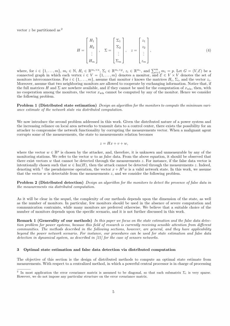
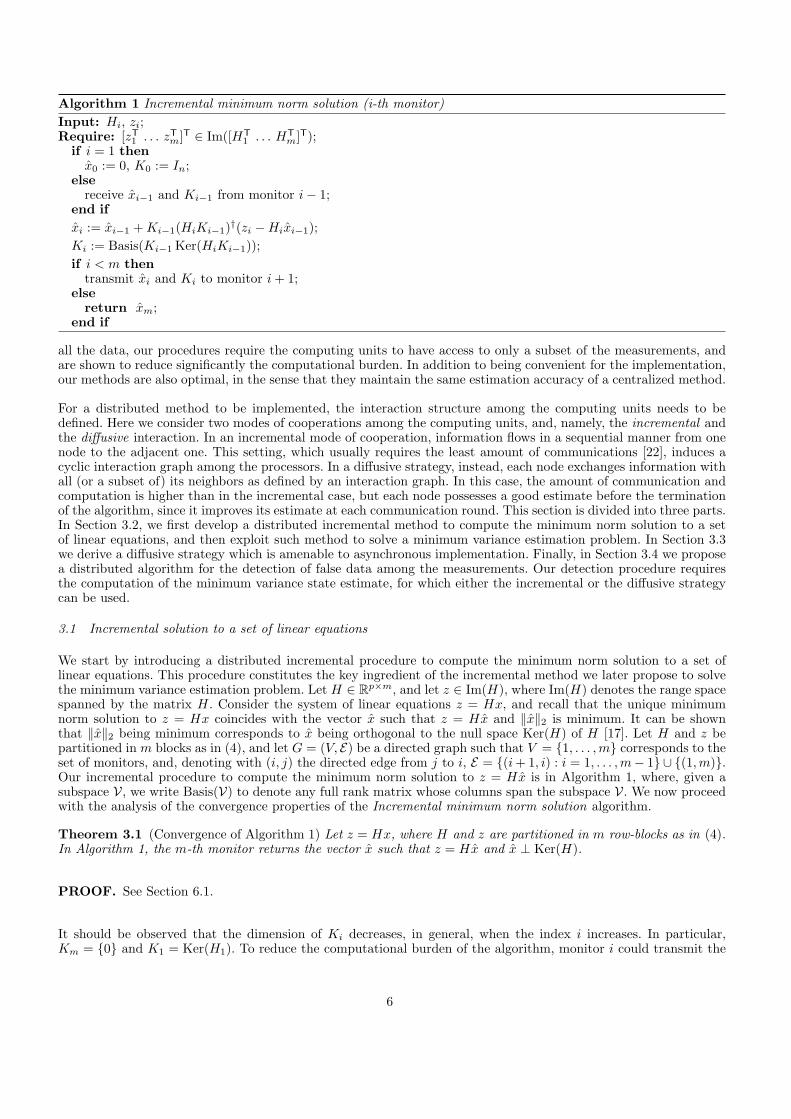
Fig. 3. For a fixed value of ε, Fig. 3(a) shows the average (over 100 tests) of the norm of the error (with respect to the networkstate) of the estimate obtained by means of Algorithm 1. The estimation error decreases with the number of measurements.Because of the presence of several control centers, our distributed algorithm processes more measurements (up to 5N) whilemaintaining the same (or smaller) computational complexity of a centralized estimation (with N measurements). Fig. 3(b)shows the residual functions computed by the 5 control centers. Since the first residual is greater than the threshold value, thepresence of false data is correctly detected by the first control center. A form of regional identification is possible by simpleidentifying the residuals above the security threshold.

let zi = Pbus,i − vi, with E[vi] = 0 and E[vivTi ] = σ2

i I, be the measurements vector of the i-th area. Finally, assumethat the i-th control center knows the matrix Hbus,i such that zi = Hbus,iθbus + vi. Then, as discussed in Section 3,the control centers can compute an optimal estimate of θbus by means of Algorithm 1 or 2. Let ni be the number ofmeasurements of the i-th area, and let N =

∑5i=1 ni. Notice that, with respect to a centralized computation of the

minimum variance estimate of the state vector, our estimation procedure obtains the same estimation accuracy whilerequiring a smaller computation burden and memory requirement. Indeed, the i-th monitor uses ni measurementsinstead of N . Let N be the maximum number of measurements that, due to hardware or numerical contraints,a control center can efficiently handle for the state estimation problem. In Fig. 3(a), we increase the number ofmeasurements taken by a control center, so that ni ≤ N , and we show how the accuracy of the state estimateincreases with respect to a single control center with N measurements.

To conclude this section, we consider a security application, in which the control centers aim at detecting the presenceof false data among the network measurements via distributed computation. For this example, we assume that eachcontrol center mesures the real power injection as well the current magnitude at some of the buses of its area. Bydoing so, a sufficient redundancy in the measurements is obtained for the detection to be feasible [1]. Suppose thatthe measurements of the power injection at the first bus of the first area is corrupted by a malignant agent. Tobe more precise, let the measurements vector of the first area be zi = zi + e1wi, where e1 is the first canonicalvector, and wi is a random variable. For the simulation we choose wi to be uniformly distributed in the interval[0, wmax], where wmax corresponds approximately to the 10% of the nominal real injection value. In order to detectthe presence of false data among the measurements, the control centers implement Algorithm 3, where, being Hthe measurements matrix, and σ, Σ the noise standard deviation and covariance matrix, the threshold value Γ ischosen as 2σ‖I−H(HTΣ−1H)−1HTΣ−1‖∞. 9 The residual functions ‖zi−Hx‖∞ are reported in Fig. 3(b). Observethat, since the first residual is greater than the threshold Γ, the control centers successfully detect the false data.Regarding the identification of the corrupted measurements, we remark that a regional identification may be possibleby simply analyzing the residual functions. In this example, for instance, since the residuals {2, . . . , 5} are below thethreshold value, the corrupted data is likely to be among the measurements of the first area. This important aspectis left as the subject of future research.

5.2 Scalability property of our finite-memory estimation technique

Consider an electrical network with (ab)2 buses, where a, b ∈ N. Let the buses interconnection structure be a twodimensional lattice, and let G be the graph whose vertices are the (ab)2 buses, and whose edges are the networkbranches. Let G be partitioned into b2 identical blocks containing a2 vertices each, and assume the presence of b2

control centers, each one responsible for a different network part. We assume the control centers to be interconnectedthrough an undirected graph. In particular, being Vi the set of buses assigned to the control center Ci, we let thecontrol centers Ci and Cj be connected if there exists a network branch linking a bus in Vi to a bus in Vj . An example

9 For a Gaussian distribution with mean µ and variance σ2, about 95% of the realizations are contained in [µ − 2σ, µ + 2σ].

15

C9 C10 C11

C13 C14 C15

C1 C2 C3 C4

C5 C6 C7 C8

C12

C16

(a)

0 2 4 6 80

2

4

0 2 4 6 80

2

4

0 2 4 6 80

2

4

0 2 4 6 80

2

4

Iteration Iteration

IterationIteration

Control center 1 Control center 6

Control center 11 Control center 15

�Err

or�

�Err

or�

�Err

or�

�Err

or�

(b)

Fig. 4. In Fig. 4(a), a two dimensional power grid with 400 buses. The network is operated by 16 control centers, each oneresponsible for a different subnetwork. Control centers cooperate through the red communication graph. Fig. 4(b) shows thenorm of the estimation error of the local subnetwork as a function of the number of iterations of Algorithm 2. The consideredmonitors are C1 ,C6, C11, and C15. As predicted by Theorem 4.1, the local estimation error becomes negligible before thetermination of the algorithm.

with b = 4 and a = 5 is in Fig. 4(a). In order to show the effectiveness of our approximation procedure, suppose thateach control center Ci aims at estimating the vector of the voltage angles at the buses in its region. We assume alsothat the control centers cooperate, and that each of them receives the measurements of the real power injected atonly the buses in its region. Algorithm 2 is implemented by the control centers to solve the estimation problem. InFig. 4(b) we report the estimation error during the iterations of the algorithm. Notice that, as predicted by Theorem4.1, each leader possess a good estimate of the state of its region before the termination of the algorithm.

6 Conclusion

Two distributed algorithms for network control centers to compute the minimum variance estimate of the networkstate given noisy measurements have been proposed. The two methods differ in the mode of cooperation of thecontrol centers: the first method implements an incremental mode of cooperation, while the second uses a diffusiveinteraction. Both methods converge in finite time, which we characterize, and they require only local measurementsand model knowledge to be implemented. Additionally, an asynchronous and scalable implementation of our diffusiveestimation method has been described, and its efficiency has been shown through a rigorous analysis and througha practical example. Based on these estimation methods, an algorithm to detect cyber-attacks against the networkmeasurements has also been developed, and its detection performance has been characterized.

APPENDIX

6.1 Proof of Theorem 3.1

PROOF. Let Hi = [HT1 · · · HT

i ]T, zi = [zT1 · · · zT

i ]T. We show by induction that zi = Hixi, Ki = Basis(Ker(Hi)),and xi ⊥ Ker(Hi). Note that the statements are trivially verified for i = 1. Suppose that they are verified up to i,then we need to show that Ki+1 = Basis(Ker(Hi+1)), xi+1 ⊥ Ker(Hi+1), and zi+1 = Hi+1xi+1.

We start by proving that Ki+1 = Basis(Ker(Hi+1)). Observe that Ker(Ki) = 0 for all i, and that

Ker(Hi+1Ki) = {v : Kiv ∈ Ker(Hi+1)}. (A-1)

Hence,

Im(Ki+1) = Im(Ki Ker(Hi+1Ki)) = Im(Ki) ∩Ker(Hi+1) = Ker(Hi) ∩Ker(Hi+1) = Ker(Hi+1).

16

We now show that xi+1 ⊥ Ker(Hi+1), which is equivalent to

xi+1 = (xi + Ki(Hi+1Ki)†(zi+1 −Hi+1xi)) ∈ Ker(Hi+1)⊥.

Note that

Ker(Hi+1) ⊆ Ker(Hi) ⇔ Ker(Hi+1)⊥ ⊇ Ker(Hi)⊥.

By the induction hypothesis we have xi ∈ Ker(Hi)⊥, and hence xi ∈ Ker(Hi+1)⊥. Therefore, we need to show that

Ki(Hi+1Ki)†(zi+1 −Hi+1xi) ∈ Ker(Hi+1)⊥.

Let w = (Hi+1Ki)†(zi+1 −Hi+1xi), and notice that w ∈ Ker(Hi+1Ki)⊥ due to the properties of the pseudoinverseoperation. Suppose that Kiw 6∈ Ker(Hi+1)⊥. Since Ker(Ki) = {0}, the vector w can be written as w = w1+w2, whereKiw1 ∈ Ker(Hi+1)⊥ and Kiw2 = Kiw − Kiw1 6= 0, Kiw2 ∈ Ker(Hi+1). Then, it holds Hi+1Kiw2 = 0, and hencew2 ∈ Ker(Hi+1Ki), which contradicts the hypothesis w ∈ Ker(Hi+1Ki)⊥. We conclude that Kiw ∈ Ker(Hi+1)⊥ ⊆Ker(Hi+1)⊥.

We now show that zi+1 = Hi+1xi+1. Because of the consistency of the system of linear equations, and because zi =Hixi by the induction hypothesis, there exists a vector vi ∈ Ker(Hi) = Im(Ki) such that zi+1 = Hi+1(xi + vi), andhence that zi+1 = Hi+1(xi +vi). We conclude that (zi+1−Hi+1xi) ∈ Im(Hi+1Ki), and finally that zi+1 = Hi+1xi+1.

6.2 Proof of Theorem 3.2

Before proceeding with the proof of the above theorem, we recall the following fact in linear algebra.

Lemma 6.1 Let H ∈ Rn×m. Then Ker((H†)T) = Ker(H).

PROOF. We first show that Ker((H†)T) ⊆ Ker(H). Recall from [2] that H = HHT(H†)T. Let x be such that(H†)Tx = 0, then Hx = HHT(H†)Tx = 0, so that Ker((H†)T) ⊆ Ker(H). We now show that Ker(H) ⊆ Ker((H†)T).Recall that (H†)T = (HT)† = (HHT)†H. Let x be such that Hx = 0, then (H†)Tx = (HHT)†Hx = 0, so thatKer(H) ⊆ Ker((H†)T), which concludes the proof.

We are now ready to prove Theorem 3.2.

PROOF. The first property follows directly from [2] (cfr. page 427). To show the second property, observe thatC† = 1

ε ((I −HH†)B)†, so that

limε→0+

εD = 0.

For the theorem to hold, we need to verify that

H† −H†B((I −HH†)B)† = (HTΣ−1H)−1HTΣ−1,

or, equivalently, that (H† −H†B((I −HH†)B)†

)HH† = (HTΣ−1H)−1HTΣ−1HH†, (A-2)

and (H† −H†B((I −HH†)B)†

)(I −HH†) = (HTΣ−1H)−1HTΣ−1(I −HH†). (A-3)

17

Consider equation (A-2). After simple manipulation, we have

H† −H†B((I −HH†)B)†HH† = H†,

so that we need to show only that

H†B((I −HH†)B)†HH† = 0.

Recall that for a matrix W it holds W † = (WTW )†WT. Then the term ((I −HH†)B)†HH† equals

(((I −HH†)B)T((I −HH†)B)

)†BT(I −HH†)HH† = 0,

because (I −HH†)HH† = 0. We conclude that equation (A-2) holds. Consider now equation (A-3). Observe thatHH†(I −HH†) = 0. Because B has full row rank, and Σ = BBT, simple manipulation yields

−HT(BBT)−1HH†B[(I −HH†)B

]†(I −HH†)B = HT(BBT)−1(I −HH†)B,

and hence

HT(BBT)−1{

I + HH†B[(I −HH†)B

]†}(I −HH†)B = 0.

Since HH† = I − (I −HH†), we obtain

HT(BBT)−1B[(I −HH†)B

]†(I −HH†)B = 0.

A sufficient condition for the above equation to be true is([(I −HH†)B

]†)T

BT(BBT)−1H = 0.

From Lemma 6.1 we have.

Ker(([

(I −AA†)B]†)T

)= Ker((I −AA†)B).

Since

(I −HH†)BBT(BBT)−1H = (I −HH†)H = 0,

we have that

HT(BBT)−1B[(I −HH†)B

]†(I −HH†)B = 0,

and that equation (A-3) holds. This concludes the proof.

References

[1] A. Abur and A. G. Exposito. Power System State Estimation: Theory and Implementation. CRC Press, 2004.[2] D. S. Bernstein. Matrix Mathematics. Princeton University Press, 2 edition, 2009.[3] R. Carli, A. Chiuso, L. Schenato, and S. Zampieri. Distributed Kalman filtering based on consensus strategies.

IEEE Journal on Selected Areas in Communications, 26(4):622–633, 2008.[4] F. S. Cattivelli, C. G. Lopes, and A. H. Sayed. Diffusion recursive least-squares for distributed estimation over

adaptive networks. IEEE Transactions on Signal Processing, 56(5):1865–1877, 2008.

18

[5] F. S. Cattivelli and A. H. Sayed. Diffusion strategies for distributed Kalman filtering and smoothing. IEEETransactions on Automatic Control, 55(9):2069–2084, 2010.

[6] Y. Censor. Row-action methods for huge and sparse systems and their applications. SIAM Review, 23(4):444–466, 1981.

[7] S. Demko, W. F. Moss, and P. W. Smith. Decay rates for inverses of band matrices. Mathematics of Computation,43(168):491–499, 1984.

[8] D. M. Falcao, F. F. Wu, and L. Murphy. Parallel and distributed state estimation. IEEE Transactions onPower Systems, 10(2):724–730, 1995.

[9] C. D. Godsil and G. F. Royle. Algebraic Graph Theory, volume 207 of Graduate Texts in Mathematics. Springer,2001.

[10] G. H. Golub and C. F. van Loan. Matrix Computations. Johns Hopkins University Press, 2 edition, 1989.[11] R. Gordon, R. Bender, and G. T. Herman. Algebraic reconstruction techniques (ART) for three-dimensional

electron microscopy and x-ray photography. Journal of theoretical Biology, 29(3):471–481, 1970.[12] W. Jiang, V. Vittal, and G. T. Heydt. A distributed state estimator utilizing synchronized phasor measurements.

IEEE Transactions on Power Systems, 22(2):563–571, 2007.[13] S. Kaczmarz. Angenaherte Auflosung von Systemen linearer Gleichungen. Bull. Acad. Polon. Sci. Lett. A,

35:355–357, 1937.[14] Y. Liu, M. K. Reiter, and P. Ning. False data injection attacks against state estimation in electric power grids.

In ACM Conference on Computer and Communications Security, pages 21–32, Chicago, IL, USA, November2009.

[15] C. G. Lopes and A. H. Sayed. Incremental adaptive strategies over distributed networks. IEEE Transactionson Signal Processing, 55(8):4064–4077, 2007.

[16] C. G. Lopes and A. H. Sayed. Diffusion least-mean squares over adaptive networks: Formulation and performanceanalysis. IEEE Transactions on Signal Processing, 56(7):3122–3136, 2008.

[17] D. G. Luenberger. Optimization by Vector Space Methods. Wiley, 1969.[18] J. Meserve. Sources: Staged cyber attack reveals vulnerability in power grid. http://cnn.com, September 26,

2007.[19] A. Monticelli. State Estimation in Electric Power Systems: A Generalized Approach. Springer, 1999.[20] NERC. Final Report on the August 14, 2003 Blackout in the United States and Canada: Causes and Recom-

mendations, April 2004. Available at http://www.nerc.com/filez/blackout.html.[21] F. Pasqualetti, R. Carli, A. Bicchi, and F. Bullo. Distributed estimation and detection under local information.

In IFAC Workshop on Distributed Estimation and Control in Networked Systems, pages 263–268, Annecy,France, September 2010.

[22] M. G. Rabbat and R. D. Nowak. Quantized incremental algorithms for distributed optimization. IEEE Journalon Selected Areas in Communications, 23(4):798–808, 2005.

[23] C. Rakpenthai, S. Premrudeepreechacharn, S. Uatrongjit, and N. R. Watson. Measurement placement for powersystem state estimation using decomposition technique. Electric Power Systems Research, 75(1):41–49, 2005.

[24] A. H. Sayed and C. G. Lopes. Adaptive processing over distributed networks. IEICE Transactions on Funda-mentals of Electronics, Communications and Computer Sciences, E90-A(8):1504–1510, 2007.

[25] I. Schizas, A. Ribeiro, and G. Giannakis. Consensus in ad hoc WSNs with noisy links - Part I: Distributedestimation of deterministic signals. IEEE Transactions on Signal Processing, 56(1):350–364, 2007.

[26] I. D. Schizas, G. Mateos, and G. B. Giannakis. Distributed LMS for consensus-based in-network adaptiveprocessing. IEEE Transactions on Signal Processing, 57(6):2365–2382, 2009.

[27] F. C. Schweppe and J. Wildes. Power system static-state estimation, Part I: Exact model. IEEE Transactionson Power Apparatus and Systems, 89(1):120–125, 1970.

[28] F. C. Schweppe and J. Wildes. Power system static-state estimation, Part II: Approximate model. IEEETransactions on Power Apparatus and Systems, 89(1):125–130, 1970.

[29] F. C. Schweppe and J. Wildes. Power system static-state estimation, Part III: Implementation. IEEE Trans-actions on Power Apparatus and Systems, 89(1):130–135, 1970.

[30] M. Shahidehpour and Y. Wang. Communication and Control in Electric Power Systems: Applicationsc ofParallel and Distributed Processing. Wiley-IEEE Press, 2003.

[31] S. S. Stankovic, M. S. Stankovic, and D. M. Stipanovic. Consensus based overlapping decentralized estimationwith missing observations and communication faults. Automatica, 45(6):1397–1406, 2009.

[32] K. Tanabe. Projection method for solving a singular system of linear equations and its applications. NumerischeMathematik, 17(3):203–214, 1971.

[33] L. Xie, Y. Mo, and B. Sinopoli. False data injection attacks in electricity markets. In IEEE Int. Conf. on SmartGrid Communications, pages 226–231, Gaithersburg, MD, USA, October 2010.

[34] L. Zhao and A. Abur. Multi area state estimation using synchronized phasor measurements. IEEE Transactionson Power Systems, 20(2):611–617, 2005.

19