distributed generation resource assessment for … generation resource assessment for long-term...
TRANSCRIPT

© 2014 Navigant Consulting, Inc.
Distributed Generation Resource Assessment for Long-Term Planning Study Supply Curve Support Prepared for: PacifiCorp
Prepared by: Karin Corfee Graham Stevens Shalom Goffri June 9, 2014 Navigant Consulting, Inc. One Market Street Spear Street Tower, Suite 1200 San Francisco, CA 94105 415.356.7100 www.navigant.com Reference No.: 171094

Page i
Table of Contents
Executive Summary ................................................................................................................... v
Key Findings ................................................................................................................................................. vii
1. Introduction ......................................................................................................................... 1-1
1.1 Methodology ......................................................................................................................................... 1-2 1.2 Report Organization ............................................................................................................................. 1-3
2. DG Technology Definitions ............................................................................................. 2-1
2.1 What is a “Distributed Generation” Source? .................................................................................... 2-1 2.1.1 Size Limits for this Study ....................................................................................................... 2-1 2.1.2 Determination of Applicable Technologies ......................................................................... 2-2 2.1.3 Solar DG Technology Definition ........................................................................................... 2-3 2.1.4 Small Distributed Wind Technology Definition ................................................................. 2-5 2.1.5 Small Scale Hydro Technology Definition ........................................................................... 2-7 2.1.6 CHP Reciprocating Engines Technology Definition ........................................................ 2-10 2.1.7 CHP Microturbine Technology Definition ........................................................................ 2-14
3. Resource Cost & Performance Assumptions ................................................................. 3-1
3.1 Photovoltaic ........................................................................................................................................... 3-1 3.1.1 Performance ............................................................................................................................. 3-1 3.1.2 Cost ........................................................................................................................................... 3-3
3.2 Small-Scale Wind .................................................................................................................................. 3-5 3.2.1 Performance ............................................................................................................................. 3-5 3.2.2 Cost ........................................................................................................................................... 3-5
3.3 Small-Scale Hydro ................................................................................................................................ 3-6 3.3.1 Performance ............................................................................................................................. 3-6 3.3.2 Cost ........................................................................................................................................... 3-7
3.4 CHP Reciprocating Engines ................................................................................................................ 3-8 3.4.1 Performance ............................................................................................................................. 3-8 3.4.2 Cost ........................................................................................................................................... 3-8
3.5 CHP Micro-turbines ............................................................................................................................. 3-9 3.5.1 Performance ............................................................................................................................. 3-9 3.5.2 Cost ........................................................................................................................................... 3-9
4. DG Market Potential and Barriers ................................................................................... 4-1
4.1 Incentives ............................................................................................................................................... 4-1 4.1.1 Federal Incentives ................................................................................................................... 4-1 4.1.2 State Incentives ........................................................................................................................ 4-1 4.1.3 Rebate Incentives ..................................................................................................................... 4-3
4.2 Market Barriers to DG Penetration ..................................................................................................... 4-4
Page ii
4.2.1 Technical Barriers .................................................................................................................... 4-4 4.2.2 Economic Barriers ................................................................................................................... 4-5 4.2.3 Legal / Regulatory Barriers .................................................................................................... 4-6 4.2.4 Institutional Barriers ............................................................................................................... 4-6
5. Methodology to Develop 2015 IRP DG Penetration Forecasts .................................. 5-1
5.1 Market Penetration Approach............................................................................................................. 5-1 5.1.1 Assess Technical Potential ..................................................................................................... 5-1 5.1.2 Simple Payback........................................................................................................................ 5-7 5.1.3 Payback Acceptance Curves .................................................................................................. 5-9 5.1.4 Market Penetration Curves .................................................................................................... 5-9 5.1.5 Scenarios ................................................................................................................................. 5-13
6. Results ................................................................................................................................... 6-1
6.1 Technical Potential ................................................................................................................................ 6-1 6.2 Overall Scenario Results ...................................................................................................................... 6-2 6.3 Results by State ..................................................................................................................................... 6-5 6.4 Results by Technology ....................................................................................................................... 6-15
Appendix A. Glossary ........................................................................................................... A-1
Appendix B. Summary Table of Results ........................................................................... B-2

Page iii
List of Figures and Tables
Figures: Figure 1-1. PacifiCorp Service Territory ............................................................................................................... vi Figure 1-2. Technical Potential Results ................................................................................................................ vii Figure 1-3. Distributed Generation Supply Curve Results, Base Case ...........................................................viii Figure 1-4. Low and High Penetration Scenario Results .................................................................................... ix Figure 1-1. PacifiCorp Service Territory ............................................................................................................. 1-2 Figure 2-1. Solar Technology Types .................................................................................................................... 2-3 Figure 2-2. PV System Applications .................................................................................................................... 2-4 Figure 2-3. Wind Turbine Examples ................................................................................................................... 2-5 Figure 2-4. U.S. SWT Sales, by Market Segment (2007-2012) ........................................................................... 2-7 Figure 2-5. Small Hydro Definition ..................................................................................................................... 2-8 Figure 2-6. Small Hydro Sizes .............................................................................................................................. 2-9 Figure 2-7. Example Small Hydro Sites, Turbines ............................................................................................ 2-9 Figure 2-8. Residential CHP Schematic ............................................................................................................ 2-11 Figure 2-9. Typical Commercial CHP System Components .......................................................................... 2-11 Figure 2-10. Reciprocating Engine Cutaway .................................................................................................... 2-12 Figure 2-11. Diesel/Gas-Fired DG Technology Applications......................................................................... 2-13 Figure 2-12. Reciprocating Engine Sizes and Fuels Used ............................................................................... 2-13 Figure 2-13. Microturbine Schematic ................................................................................................................ 2-14 Figure 2-14. Example Micro-turbines (Capstone Turbine Corporation) ...................................................... 2-14 Figure 3-1. Example Solar Panels: Mono-crystalline and Poly-crystalline ................................................... 3-1 Figure 3-2. Typical Crystalline Solar Cell Cross Section .................................................................................. 3-2 Figure 3-3. Example Solar Module Power Warranty ........................................................................................ 3-2 Figure 3-4. Photovoltaic Module Price Trends. ................................................................................................. 3-4 Figure 3-5. Hydropower project capacity factors in the Clean Development Mechanism .......................... 3-6 Figure 4-1. Net Metering Policies in the U.S. ..................................................................................................... 4-6 Figure 4-2. US Benchmark Interest Rate ............................................................................................................. 4-7 Figure 5-1. US Wind Resource Map .................................................................................................................... 5-6 Figure 5-2. Payback Acceptance Curves ............................................................................................................. 5-9 Figure 5-3. Fisher-Pry Market Penetration Dynamics .................................................................................... 5-11 Figure 5-4. DG Market Penetration Curves Used ........................................................................................... 5-12 Figure 6-1. Technical Potential Results ............................................................................................................... 6-1 Figure 6-2. Base Case Results ............................................................................................................................... 6-2 Figure 6-3. Low Penetration Scenario Results ................................................................................................... 6-3 Figure 6-4. High Penetration Scenario Results .................................................................................................. 6-4 Figure 6-5. Utah Base Case Results ..................................................................................................................... 6-5 Figure 6-6. Utah Residential PV Market Drivers ............................................................................................... 6-7 Figure 6-7. Utah Small Commercial PV Market Drivers .................................................................................. 6-8 Figure 6-8. Utah Near-Term PV Projections ...................................................................................................... 6-9 Figure 6-9. California Base Case Results .......................................................................................................... 6-10 Figure 6-10. Idaho Base Case Results ................................................................................................................ 6-11

Page iv
Figure 6-11. Oregon Base Case Results ............................................................................................................. 6-12 Figure 6-12. Washington Base Case Results ..................................................................................................... 6-13 Figure 6-13. Wyoming Base Case Results ........................................................................................................ 6-14 Figure 6-14. Reciprocating Engines Base Case Results ................................................................................... 6-15 Figure 6-15. Micro-turbines Base Case Results ................................................................................................ 6-16 Figure 6-16. Small Hydro Base Case Results ................................................................................................... 6-17 Figure 6-17. Photovoltaics Base Case Results .................................................................................................. 6-18 Figure 6-18. Photovoltaics Residential Base Case Results .............................................................................. 6-19 Figure 6-19. Photovoltaic Commercial Base Case Results ............................................................................. 6-20 Figure 6-20. Small Wind Base Case Results ..................................................................................................... 6-21 Figure 6-21. Small Wind Residential Results ................................................................................................... 6-22 Figure 6-22. Small Wind Commercial Results ................................................................................................. 6-23 Tables: Table 2-1. PacifiCorp Net Metering Limits ........................................................................................................ 2-1 Table 2-2. Applicable DG Technologies ............................................................................................................. 2-2 Table 2-3. Common Applications for Small Wind Systems ............................................................................. 2-6 Table 3-1. PV Installation and Maintenance Cost Assumptions ..................................................................... 3-3 Table 3-2. Small Scale Wind Cost Assumptions ................................................................................................ 3-5 Table 3-3. Small Scale Hydro Cost Assumptions .............................................................................................. 3-7 Table 3-4. CHP Reciprocating Engines Cost Assumptions .............................................................................. 3-8 Table 3-5. CHP Microturbine Cost Assumptions .............................................................................................. 3-9 Table 4-1. State Tax Incentives ............................................................................................................................. 4-2 Table 4-2. Rebate Incentives ................................................................................................................................. 4-3 Table 5-1. CHP Technical Potential ..................................................................................................................... 5-2 Table 5-2. CHP Install Base .................................................................................................................................. 5-3 Table 5-3. Small Hydro Technical Potential Results ......................................................................................... 5-4 Table 5-4. PV System Size per Customer Class Example (Utah) ..................................................................... 5-5 Table 5-5. Utah PV Technical Potential............................................................................................................... 5-5 Table 5-6. Small Wind Technical Potential Results ........................................................................................... 5-7 Table 5-7. Residential Tax Rates .......................................................................................................................... 5-8 Table 5-8. Commercial Tax Rate .......................................................................................................................... 5-8 Table 5-9. Scenario Variable Modifications ...................................................................................................... 5-13
Page v
Disclaimer
This report was prepared by Navigant Consulting, Inc. exclusively for the benefit and use of PacifiCorp and/or its affiliates or subsidiaries. The work presented in this report represents our best efforts and judgments based on the information available at the time this report was prepared. Navigant Consulting, Inc. is not responsible for the reader’s use of, or reliance upon, the report, nor any decisions based on the report. NAVIGANT CONSULTING, INC. MAKES NO REPRESENTATIONS OR WARRANTIES, EXPRESSED OR IMPLIED. Readers of this report are advised that they assume all liabilities incurred by them, or third parties, as a result of their reliance on this report, or the data, information, findings and opinions contained in this report. June 9, 2014

Page vi
Executive Summary
Navigant Consulting, Inc. (Navigant) prepared this Distributed Generation Resource Assessment for Long-term Planning Study on behalf of PacifiCorp. A key objective of this research is to assist PacifiCorp in developing distributed generation resource penetration forecasts to support its 2015 Integrated Resource Plan (IRP). The purpose of this study is to project the level of distributed resources PacifiCorp’s customers might install over the next twenty years. Navigant evaluated five Distributed Generation resources in detail in this report:
1. Photovoltaic (Solar)
2. Small Scale Wind
3. Small Scale Hydro
4. Combined Heat and Power Reciprocating Engines
5. Combined Heat and Power Micro-turbines Other technologies were excluded as they were: 1) analyzed elsewhere for the IRP; 2) are too large to be considered “Distributed” resources; or 3) are not economically viable on a large scale. Project sizes were restricted to be less than the size limits of the relevant state net metering regulation, i.e. less than 2 MW in Oregon and Utah; <1 MW in CA; <100 kW in ID and WA; and <25 kW in WY. Distributed generation technical potential and market penetration was estimated by technology and by geography, i.e. the portion of the individual states that are in PacifiCorp’s service territory, including parts of California, Idaho, Oregon, Utah, Washington, and Wyoming (Figure 1-1).
Figure 1-1. PacifiCorp Service Territory1
1 http://www.pacificorp.com/content/dam/pacificorp/doc/About_Us/Company_Overview/Service_Area_Map.pdf
Page vii
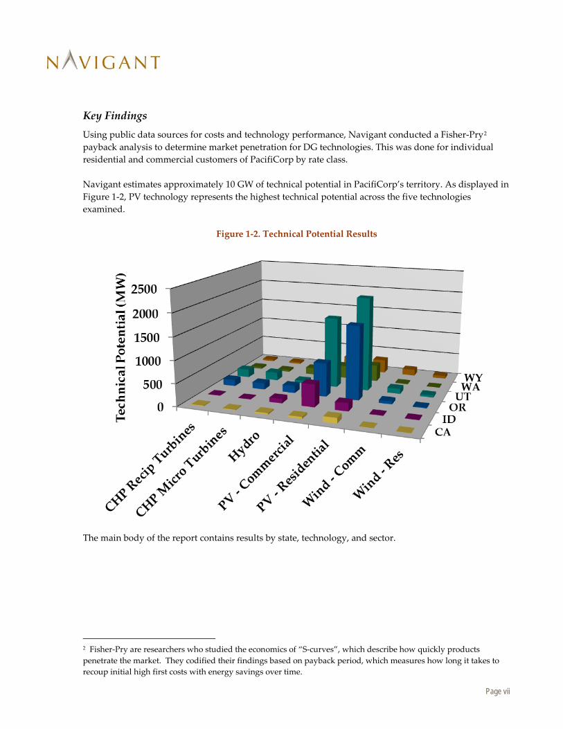
Key Findings Using public data sources for costs and technology performance, Navigant conducted a Fisher-Pry2 payback analysis to determine market penetration for DG technologies. This was done for individual residential and commercial customers of PacifiCorp by rate class. Navigant estimates approximately 10 GW of technical potential in PacifiCorp’s territory. As displayed in Figure 1-2, PV technology represents the highest technical potential across the five technologies examined.
Figure 1-2. Technical Potential Results
The main body of the report contains results by state, technology, and sector.
2 Fisher-Pry are researchers who studied the economics of “S-curves”, which describe how quickly products penetrate the market. They codified their findings based on payback period, which measures how long it takes to recoup initial high first costs with energy savings over time.

Page viii
Our overall results reflect our base case market penetration analysis, and we found that the near term outlook is roughly 50 MW in 2019 and reaches 900 MW by 2034, the end of the IRP period (Figure 1-3).
Figure 1-3. Distributed Generation Supply Curve Results, Base Case

Page ix
In the low and high penetration cases, 33 MW and 95MW penetration is achieved by 2019, rapidly expanding thereafter to achieve 290 and 2630 MW of penetration in 2034, respectively (Figure 1-4).
Figure 1-4. Low and High Penetration Scenario Results
Page 1-1
1. Introduction
Navigant Consulting, Inc. (Navigant) prepared this Distributed Generation Resource Assessment for Long-term Planning Study on behalf of PacifiCorp. A key objective of this research is to assist PacifiCorp in developing distributed generation resource penetration forecasts to support its 2015 Integrated Resource Plan (IRP). The purpose of this study is to project the level of distributed resources PacifiCorp’s customers will install over the next 20 years. Navigant evaluated five distributed generation resources in detail in this report:
1. Photovoltaic (Solar)
2. Small Scale Wind
3. Small Scale Hydro
4. Combined Heat and Power Reciprocating Engines
5. Combined Heat and Power Micro-turbines Other technologies were excluded as they were: 1) analyzed elsewhere for the IRP; 2) are too large to be considered “Distributed” resources; or 3) are not economically viable on a large scale. Project sizes were restricted to be less than the size limits of the relevant state net metering regulation, i.e. less than 2 MW in Oregon and Utah; <1 MW in CA; <100 kW in ID and WA; and <25 kW in WY. Distributed generation technical potential and market penetration was estimated by technology and by geography, i.e. the portion of the individual states that are in PacifiCorp’s service territory, including parts of California, Idaho, Oregon, Utah, Washington, and Wyoming (Figure 1-1).

Page 1-2
Figure 1-1. PacifiCorp Service Territory3
1.1 Methodology In assessing the technical and market potential of each distributed generation (DG) resource and opportunity in PacifiCorp’s service area, the study considered a number of key factors, including:
• Technology maturity, costs, & future cost improvements
• Industry practices, current and expected
• Net metering policies
• Tax incentives
• Utility rebates
• O&M costs
• Historical performance, and expected performance improvements
• Availability of DG resources
• Consumer behavior and market penetration
3 http://www.pacificorp.com/content/dam/pacificorp/doc/About_Us/Company_Overview/Service_Area_Map.pdf

Page 1-3
Using public data sources for costs and technology performance, Navigant conducted a Fisher-Pry4 payback analysis to determine market penetration for DG technologies. This was done for individual residential and commercial customers of PacifiCorp by rate class. A five-step process was used to determine the IRP penetration scenarios for DG resources:
1. Assess a Technology’s Technical Potential: Technical potential is the amount of a technology that can be physically installed without considering economics.
2. Calculate First Year Simple Payback Period for Each Year of Analysis: From past work in projecting the penetration of new technologies, Navigant has found that Simple Payback Period is the best indicator of uptake. Navigant used all relevant federal, state, and utility incentives in its calculation of paybacks, including their expiration dates.
3. Project Ultimate Adoption Using Payback Acceptance Curves: Payback Acceptance Curves estimate what percentage of a market will ultimately adopt a technology, but do not factor in how long adoption will take.
4. Project Market Penetration Using Market Penetration Curves: Market penetration curves factor in market and technology characteristics to project how long adoption will take.
5. Project Market Penetration under Different Scenarios. In addition to the Base Case scenario, a High and Low Case scenarios were evaluated that used different 20-year average cost assumptions, performance assumptions, and electricity rate assumptions.
Navigant examined the cost of electricity from the customer perspective, called “levelized cost of energy” (LCOE). A LCOE calculation takes total installation costs, incentives, annual costs such as maintenance and financing costs, and system energy output, and calculates a net present value $/kWh for electricity which can be compared to current retail prices. A simple payback calculation involves the same analysis conducted for year 1, and calculates the first year costs divided by first year energy savings to see how long it will take for the investment to pay for itself. Navigant has used LCOE and payback analyses to examine consumer decisions as to whether purchase of distributed resources makes economic sense for these customers, and then projects DG penetration based on these analyses.
1.2 Report Organization The remainder of this report is organized as follows:
• Distribution Generation Technology Definitions
• Resource Cost & Performance Assumptions
• DG Market Potential and Barriers
• Market Barriers to DG
• Methodology to Develop 2015 DG Penetration Forecasts
4 Fisher-Pry are researchers who studied the economics of “S-curves”, which describe how quickly products penetrate the market. They codified their findings based on payback period, which measures how long it takes to recoup initial high first costs with energy savings over time.

Page 1-4
• Results
• Appendix A: Glossary.

Page 2-1
2. DG Technology Definitions
2.1 What is a “Distributed Generation” Source? Distributed generation (DG) sources provide on-site energy generation and are generally of relatively small size, usually no larger than the amount of power used at a particular location.
2.1.1 Size Limits for this Study
For this study, the DG resources must meet the size requirements for net metering for the six states of PacifiCorp’s service territory, as installations that take into account net metering benefits are likely to be most economical. These size requirements are generally less than 2 MW, per Table 2-1 below.
Table 2-1. PacifiCorp Net Metering Limits
State Net Metering Size Limits
CHP? Net Metering Credits5 Source
CA6 1 MW, unless university/local government owned (5 MW)
N Retail rate7 http://www.cpuc.ca.gov/ PUC/energy/DistGen/netmetering.htm
ID8 100 kW non-residential 25 kW res / small commercial
N Retail rate for residential / small commercial 85% avoided cost rate for all others
http://www.rockymountainpower.net/env/nmcg.html
OR9 2 MW non-residential 25 kW residential
N Retail rate OR Revised Statues 757.300; Or Admin R. 860-039; OR Admin R. 860-022-0075
UT10 2 MW non-residential 25 kW residential
Y • Retail rate for residential/ small commercial
• Large commercial/ industrial with demand charges choose between avoided cost rate or alternative rate (FERC Form No. 1)
http://energy.utah.gov/funding-incentives/
WA11
100 kW Y Retail rate Rev. Code Wash. § 80.60
WY12 25 kW N Retail rate http://psc.state.wy.us/
5 The NEM credit for DG generation used to nullify or offset purchases from the utility. 6 http://www.cpuc.ca.gov/PUC/energy/DistGen/netmetering.htm 7 The rate block of the energy component of retail rates that the DG customer is able to avoid paying as a result of each kWh of DG production to which NEM applies. 8 http://www.rockymountainpower.net/env/nmcg.html 9 OR Revised Statues 757.300; Or Admin R. 860-039; OR Admin R. 860-022-0075 10 http://www.energy.utah.gov/renewable_energy/renewable_incentives.... 11 Rev. Code Wash. § 80.60

Page 2-2
Net Metering applies to all DG technologies under consideration, with the possible exception of combined heat and power (CHP), as notated in Column 3 of Table 2-1.
2.1.2 Determination of Applicable Technologies
Technologies considered for this study include commercialized technologies that are generally installed in system sizes smaller than the net metering limits designated in Table 2-1, with a focus on technologies that are achieving market penetration in PacifiCorp’s service territory (namely solar and wind). Table 2-2 below lists potentially applicable technologies, which ones were included (those in grey), and the reasons why a number of technologies were not included at this time. Note, future IRP’s may include consideration of more technologies, especially those upon the cusp of commercialization (such as fuel cells), but resource constraints excluded them at present. Nevertheless, we believe we have captured the major trends and DG technologies that will impact PacifiCorp over the next decade, as newer technologies will take a long time to overcome commercialization challenges and significantly penetrate the market.
Table 2-2. Applicable DG Technologies
Distributed Generation Technology 2013 Net
Meter Customers
Included in this DG Study?
Comment
Photovoltaic ~94% Yes Highest level of DG market penetration Small Scale Wind ~6% Yes Technical potential is potentially high,
especially in WY Small Hydro
Yes Technical potential is relatively high in the Pacific Northwest
CHP [Identified in 2013 IRP CHP Memo]
Reciprocating Engines
Yes Largest market penetration, commercial technology
Micro-turbines Yes Newer technology Natural Gas Turbines
No Turbine sizes generally larger than 2 MW
Fuel Cells No Non-commercial with limited market penetration
Industrial Biomass
No Large scale, does not apply to DG
Anaerobic Digester (AD) Biogas
No Similarly, AD is not generally economic on a small scale
Solar Hot Water [see 2013 IRP SHW Memo ]
No Solar Hot Water is included in the Demand Side Management study
12 http://psc.state.wy.us/

Page 2-3
2.1.3 Solar DG Technology Definition
There are primarily two methods of converting sunlight into electricity: solar electric (photovoltaic), and solar thermal. These are depicted below in Figure 2-1.
Figure 2-1. Solar Technology Types
Solar thermal technologies, which concentrate energy to raise the temperature of a heat transfer fluid, usually require system sizes of 50MW or higher to be economical, so we have excluded them from further consideration. Commercialized solar electric technologies include crystalline silicon (~90% of the market), and thin film (~10% of the market). Other solar technologies include concentrating photovoltaics (CPV), and photovoltaics with tracking. For purposes of this study, we define photovoltaics to be crystalline or thin film module technologies that are mounted at either a fixed angle (usually 30-45 degrees) to a pitched roof, or mounted at a fixed angle (usually 5-10 degrees) on a flat rooftop, as most “less than 2 MW” applications are typically rooftop mounted. Concentrating photovoltaic technologies are currently uneconomic, with little market penetration, and tracking technologies are used mostly on large-scale fields (>2 MW project scale). Photovoltaics can be used at many system sizes and voltages, sometimes called applications (see Figure 2-2 below). For purposes of this study, we are considering grid-connected applications only, as PacifiCorp is interested in the distributed resources that will impact future resource decisions, and off-grid applications are by definition not connected to PacifiCorp’s electrical grid. In addition, we exclude large central/substation applications that operate at transmission voltages because these projects are

Page 2-4
almost all done at larger than 2 MW scale, the net metering limit. This excludes a few large industrial rate consumers from this study.
Figure 2-2. PV System Applications

Page 2-5
2.1.4 Small Distributed Wind Technology Definition13
Wind technologies produce electricity by using a tower to hold up a multi-bladed structure. Wind spins the blades and generated power in a wind turbine. Sizes can range from very large structure (100’s of feet tall), to much smaller (10s of feet tall), as shown in Figure 2-3.
Figure 2-3. Wind Turbine Examples
Large Med Small Small Small wind systems are most commonly defined as those with rated nameplate capacities between 1 kW and 100 kW; however, some groups include small wind turbines (SWT) of up to 500 kW in that category. For purposes of keeping power classes consistent when comparing historical and forecast annual installed data, Navigant uses the range of SWTs less than 100kW, unless otherwise noted. The primary focus of this report is on-grid-connected systems, as these systems will impact PacifiCorp’s future load. A small wind system consists of, as necessary, a turbine, tower, inverter, wiring, and foundation, and these systems can be used for both grid-tied and off-grid applications. Micro-wind is a subset of the small wind classification and is generally defined as turbines of less than 1 kW in capacity. These units are typically used in off-grid applications such as battery charging, providing electricity on sailboats and recreational vehicles, and for pumping water on farms and ranches. We consider micro-wind applications to be a part of the small wind residential segment. Community wind is another distributed wind category; it is typically a larger-scale project that includes one or several medium- to large-scale turbines to create a small wind farm with total capacity in the range of 1 MW to 20 MW. In this arrangement, the wind farm is at least majority-owned by the end users. Community wind projects in Minnesota and Iowa, for example, have utilized 1 MW-plus turbines. For comparison, community wind installations made up approximately 5.6% of total U.S. installed wind capacity in 2010 and 6.7% in 2011. However, because community wind projects tend to be on the large size, over the above net meter limits, these projects are considered to be part of the large wind market, and are not considered DG.
13 Note, this section is taken from “Small Wind Power: Demand Drivers, Market Barriers, Technology Issues, Competitive Landscape, and Global Market”, a Navigant Research report, 1Q 2013, by Dexter Gauntlett and Mackinnon Lawrence.

Page 2-6
Overall, small wind represents far less than 1% of U.S. annual installed wind capacity. Small wind turbines (SWT) are classified as either horizontal-axis or vertical-axis. Horizontal-axis wind turbines (HAWTs) must be installed at a height of 60 ft. to 150 ft. (usually on a tower) in order to access sufficient unhindered wind to be efficient. They can also be installed atop tall buildings. Unlike HAWTs, vertical-axis wind turbines (VAWTs) are designed to utilize more turbulent wind patterns such as those found in urban areas [an example of this type of turbine is shown at the far right of Figure 2-3]. VAWTs are associated with rooftop installations and are sometimes integrated into a building’s architecture. In general, VAWTs are much less efficient than HAWTs, but the actual output of any turbine depends on wind conditions at the site. Most experts agree that, in light of their economics and energy output, urban SWTs have yet to constitute a viable or sustainable market – at least with current designs. Table 2-3 illustrates common SWT applications based on turbine size. For this study, only the on-grid applications in blue are being modeled and considered further.
Table 2-3. Common Applications for Small Wind Systems
Rated System Power
Wind-diesel Wind Mini-farm Wind hybrid Single Wind Turbine
Wind home system Build Integrated < 1 kW X X X X X X X X X X X 1 kW- 7 kW X X X X X X X X X X X X X X 7 - 50 kW X X X X X X X X X X 50 - 100 kW X X X X X
Small wind applications Sa
ilboa
ts
Sign
alin
g
Stre
et la
mp
Rem
ote
hous
es
Farm
s
Wat
er P
umpi
ng
Seaw
ater
Des
alin
atio
n
Vill
age
Pow
er
Min
i-gri
d
Stre
et L
amp
Build
ing
Roo
ftop
Dw
ellin
gs
Publ
ic C
ente
rs
Car
Par
king
Indu
stri
al
Farm
s
Off-grid On-grid
Another picture of how SWT size varies with application is shown in Figure 2-4 from a recent market survey conducted by Pacific Northwest Laboratory in 2013. Off-grid small turbines tend to be .1-.9 kW in size; residential turbine sizes vary from 1-10 kW, mimicking residential loads; and commercial small wind markets use a broader 11-100 kW in turbine sizes. Note, also that the total small wind capacity additions for the country in 2012 was ~54 MW, which is relatively low compared to the over 13000 MW amount of total wind power installed in the US in 201214.
14 2012 Wind Technologies Market Report, US Department of Energy and Lawrence Berkeley Livermore Laboratory.

Page 2-7
Figure 2-4. U.S. SWT Sales, by Market Segment (2007-2012)15
2.1.5 Small Scale Hydro Technology Definition
In assessing hydro potential, Navigant references a number of U.S. Department of Energy (DOE) reports that inventory the potential for small- and large-scale hydro:`
• “Assessment of Natural Stream Sites for Hydroelectric Dams in the Pacific Northwest Region”, Hall, Verdin, and Lee, March 2012, Idaho National Laboratory, INL/EXT-11-23130
• “Feasibility Assessment of the Water Energy Resources of the United States for New Low Power and Small Hydro Classes of Hydroelectric Plants”, US Department of Energy, DOE-ID-11263, January 2006
• “Water Energy Resources of the United States with Emphasis on Low Head/Low Power Resources”, US Department of Energy, DOE.UD-11111, April 2004
The 2012 report details data for the Pacific Northwest Region, which covers Oregon, Washington, Idaho; the older report in 2006 represents the best information available for Utah, Wyoming, and California. DOE has also posted GIS software on-line for these hydro resources, especially the Pacific Northwest, which has the highest technical potential. These reports define high power as > 1 MW, low power as < 1 MW, high-head as > 30 feet, and low head as < 30 feet. For the Pacific Northwest, we had access to the actual technical potential measurements by
15 2012 Market Report on Wind Technologies in Distributed Applications, Aug 2013, Pacific Northwest National Laboratory, Orrell et al.

Page 2-8
site, so defined small hydro as less than 2 MW, the net metering limit, to be consistent with the rest of the study. As an example, Figure 2-5 shows the sites assessed in the Pacific Northwest, where each blue dot represents a potential site. The red zone below 2 MW represents our definition of small hydro for purposes of this study. It captures both high-head, low flow streams (i.e. large drops/waterfalls with small amounts of water), to low head, high flow streams (i.e. small drops with large amounts of water flowing), that each can add up to 2 MW of power produced annually. The studies examined estimated annual mean flow and power rates using state of the art digital elevation models and rainfall/weather records, and represent a maximum ideal power potential that may differ from specific site assessments that will include exact stream geometry, economic considerations, etc.
Figure 2-5. Small Hydro Definition16
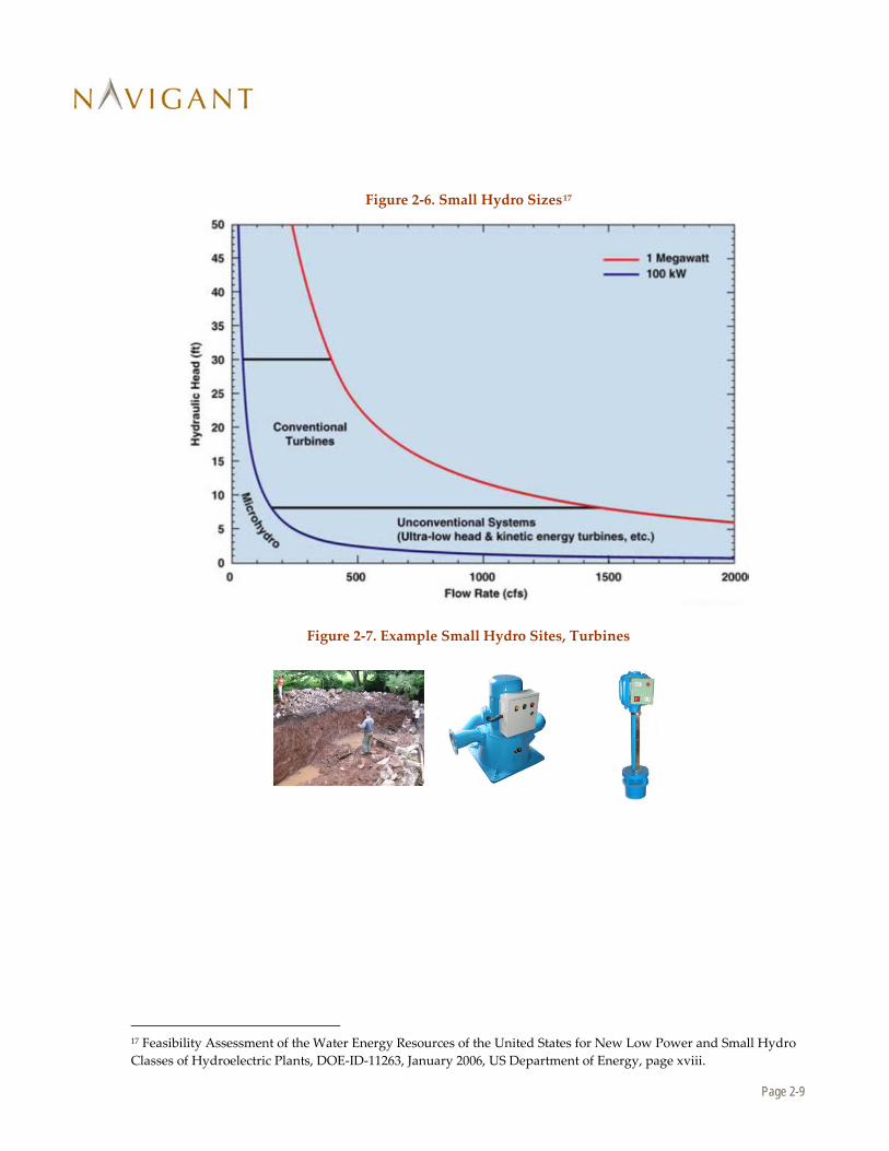
Figure 2-6 shows the hydraulic head vs. flow rates, and how these relate to conventional turbine designs, micro-hydro designs, and unconventional systems (ultra low head, kinetic energy turbines, etc.). Our study includes assessment of all of these technologies, as long as the estimated power produced annually is below 2 MW. Electric power is produced when water flows through a turbine, which spins a generator/alternator to generate electricity directly. See Figure 2-6 for an example site and a few representative turbine styles.
16 Figure 26, “Assessment of Natural Stream Sites for Hydroelectric Dams in the Pacific Northwest Region”, Douglas Hall, Kristine Verdin, Randy Lee, March 2012.
Page 2-9
Figure 2-6. Small Hydro Sizes17
Figure 2-7. Example Small Hydro Sites, Turbines
17 Feasibility Assessment of the Water Energy Resources of the United States for New Low Power and Small Hydro Classes of Hydroelectric Plants, DOE-ID-11263, January 2006, US Department of Energy, page xviii.

Page 2-10
2.1.6 CHP Reciprocating Engines Technology Definition
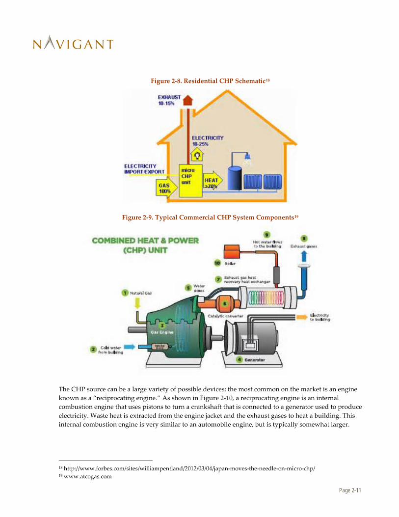
In a combined heat and power application, a small CHP power source will burn a fuel to produce both electricity and heat. In many applications, the heat is transferred to water, and this hot water is then used to heat a building (or sets of buildings, in the case of college or business campuses). The heat transfer fluid can also be steam, heating the building via radiators. Finally, in a factory setting the heat generated can be used directly in industrial processes (such a furnaces, etc.) Figure 2-8 and Figure 2-9 show example schematics for these systems.
Page 2-11
Figure 2-8. Residential CHP Schematic18
Figure 2-9. Typical Commercial CHP System Components19
The CHP source can be a large variety of possible devices; the most common on the market is an engine known as a “reciprocating engine.” As shown in Figure 2-10, a reciprocating engine is an internal combustion engine that uses pistons to turn a crankshaft that is connected to a generator used to produce electricity. Waste heat is extracted from the engine jacket and the exhaust gases to heat a building. This internal combustion engine is very similar to an automobile engine, but is typically somewhat larger.
18 http://www.forbes.com/sites/williampentland/2012/03/04/japan-moves-the-needle-on-micro-chp/ 19 www.atcogas.com

Page 2-12
Figure 2-10. Reciprocating Engine Cutaway20
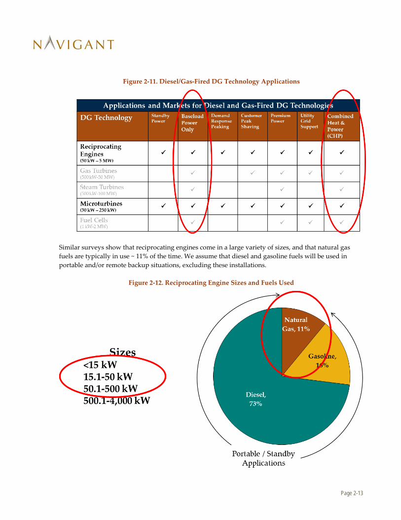
Navigant Research has done extensive surveys of diesel and gas-fired DG technology markets, and has found that ~80% of reciprocating engine sales are estimated to be for portable (i.e. for construction) and/or backup power applications21. For purposes of this study, these two applications are excluded because neither application would provide base-load power for PacifiCorp. Our main focus is therefore on the applications shown in Figure 2-11, namely base-load power applications and CHP applications.
20 a2dialog.wordpress.com 21 “Diesel Generator Sets: Distributed Reciprocating Engines for Portable, Standby, Prime, Continuous, and Cogeneration Applications”, 1Q2013, Dexter Gauntlett, Navigant Research.
Page 2-13
Figure 2-11. Diesel/Gas-Fired DG Technology Applications
Similar surveys show that reciprocating engines come in a large variety of sizes, and that natural gas fuels are typically in use ~ 11% of the time. We assume that diesel and gasoline fuels will be used in portable and/or remote backup situations, excluding these installations.
Figure 2-12. Reciprocating Engine Sizes and Fuels Used

Page 2-14
2.1.7 CHP Microturbine Technology Definition
The definition for the microturbine category is equivalent to that for reciprocating engines above, except that the CHP source is a microturbine rather than a reciprocating engine. A schematic of this type of device is shown in Figure 2-13.
Figure 2-13. Microturbine Schematic22
The microturbine uses natural gas to start a combustor, which drives a turbine. The turbine, in turn drives an AC generator and compressor, and the waste heat is exhausted to the user. The device therefore produces electrical power from the generator, and waste heat to the user. Emissions tend to be very low, allowing installation in locations with strict emissions controls, and they tend to have fewer moving parts than reciprocating engines, which they compete with directly in various applications. Navigant used the performance specifications of a typical microturbine design as profiled in various market reports23,24. Figure 2-14 shows one example offering.
Figure 2-14. Example Micro-turbines (Capstone Turbine Corporation)
22 www.understandingchp.com 23 “Catalog of CHP Technologies”, U.S. Environmental Protection Agency, December 2008 24 “Combined Heat and Power: Policy Analysis and Market Assessment 2011-2030”, ICF, February 2012
Page 3-1
3. Resource Cost & Performance Assumptions
3.1 Photovoltaic
3.1.1 Performance
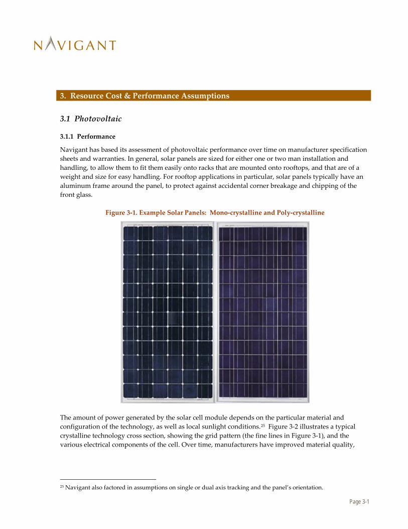
Navigant has based its assessment of photovoltaic performance over time on manufacturer specification sheets and warranties. In general, solar panels are sized for either one or two man installation and handling, to allow them to fit them easily onto racks that are mounted onto rooftops, and that are of a weight and size for easy handling. For rooftop applications in particular, solar panels typically have an aluminum frame around the panel, to protect against accidental corner breakage and chipping of the front glass.
Figure 3-1. Example Solar Panels: Mono-crystalline and Poly-crystalline
The amount of power generated by the solar cell module depends on the particular material and configuration of the technology, as well as local sunlight conditions.25 Figure 3-2 illustrates a typical crystalline technology cross section, showing the grid pattern (the fine lines in Figure 3-1), and the various electrical components of the cell. Over time, manufacturers have improved material quality,
25 Navigant also factored in assumptions on single or dual axis tracking and the panel’s orientation.

Page 3-2
material types, processes, and optics to generate slightly more power in the same area. For mature technologies, these gains have been on the order of .1% / year for mainstream commercial cells26.
Figure 3-2. Typical Crystalline Solar Cell Cross Section
A photovoltaic module will experience some slight amount of degradation over time, as the wires in the cells age and oxidation increases resistance, as differential thermal expansion ages the cells, etc. In the industry, it is an industry standard to offer a limited power output warranty which covers this degradation. An example warranty is shown in Figure 3-3.
Figure 3-3. Example Solar Module Power Warranty
In summary, we assume .1% efficiency gains over the next 20 years, mimicking solar technology performance over the last 20 years; and assume a .7% annual degradation rate in keeping with current module warranties that guarantee 80% power after 25 years.
26 Based on February Photon International’s annual survey of PV module specification sheets over the last twenty years.
b) 25 Year Limited Power Output Warranty In addition, Trina Solar warrants that for a period of twenty-five years commencing on the Warranty Start Date loss of power output of the nominal power output specified in the relevant Product Data Sheet and measured at Standard Test Conditions (STC) for the Product(s) shall not exceed: For Polycrystalline Products (as defined in Sec. 1 a): 2.5 % in the first year,
thereafter 0.7% per year, ending with 80.7% in the 25th year after the Warranty Start Date,
For Monocrystalline Products (as defined in Sec. 1 b): 3.5 % in the first year, thereafter 0.68% per year, ending with 80.18% in the 25th year after the Warranty Start Date.
Page 3-3
3.1.2 Cost
Amalgamating a number of public sources of data regarding PV installed and maintenance costs with our own private sources and internal databases, we used the following assumptions and sources for these costs:
Table 3-1. PV Installation and Maintenance Cost Assumptions
Photovoltaic DG Resource Costs
Units Baseline 2013 (nominal $)
Sources Residential Commercial
Installed Cost
$/kWDC $4000 $3125
• Navigant Research market estimates • Photovoltaic System Pricing Trends:
Historical, Recent, and Near - Term Projections, 2013 Edition, NREL/LBNL
Fixed O&M
$/kW-Yr $23 $25
• Navigant Research market estimates • Addressing Solar Photovoltaic
Operations and Maintenance Challenges, 2010, EPRI
• True South Renewables, Solar Plaza O&M Meeting 2014
Module prices have come down dramatically over the last few decades, as the brown line shows in Figure 3-4. This has impacted system prices sharply, as module price has traditionally been ~50% of total system price.

Page 3-4
Figure 3-4. Photovoltaic Module Price Trends27.
In our base case, Navigant assumes that PV annual system installation cost reductions will continue at the same rate as has occurred over the last ten years. Plotting the data from the above graph, this equals 4.7% cost reduction annually for commercial installations, and slightly higher 5.3% cost reduction for residential installations. Note, a higher proportion of installation costs have become non-module costs (installation labor, design, permitting, etc.) recently, and the U.S. is a relatively immature market relative to scale regarding these non-module factors. Our expectation is that these non-module costs will start to mimic more mature markets such as Germany where costs are demonstrably lower28. However, costs likely cannot be reduced at such a relatively high rate forever. Navigant assumes that DOE’s modeled System Overnight Capital Cost will form a floor for future PV system prices, reaching 1.80 $/WpDC (commercial), and 2.10 $/WpDC (residential). For our high and low penetration cases, we vary these cost projections by +/- 10%.
27 Photovoltaic System Pricing Trends: Historical, Recent, and Near-Term Projections, 2013 Edition”,Feldman et al, NREL/LBNL, PR-6A20-60207 28 “Why are Residential PV Prices in Germany So Much Lower Than in the United States?” A Scoping Analysis”, Joachim Seel, Galen Barbose, and Ryan Wiser, Lawrence Berkeley National Laboratory, Feb 2013, sponsored by SunShot, US Department of Energy.

Page 3-5
3.2 Small-Scale Wind
3.2.1 Performance
Large-scale wind has dramatically improved system capacity factor over 10% over the last two decades29. This has reflected larger and larger turbine sizes, improvements in air flow modeling, blade angle control, indirect to direct drive innovations, etc. Small wind suffers from (a) size limitations, and (b) wind strength close to the earth tends to be much lower, Navigant assumes small wind system performance improvements will be roughly half of those achieved by its bigger cousins to reflect these factors and physical limits. We therefore assume that capacity factors will change from around 20% in 2013 to approximately 33% in 2034.
3.2.2 Cost
The most recent public cost data that we could find regarding small wind installed cost and maintenance costs are shown in Table 3-2:
Table 3-2. Small Scale Wind Cost Assumptions
Small Scale Wind
DG Resource Costs
Units Baseline
2013 (nominal $)
Sources
Installed Cost (Residential)
$/kW
$6960 Capacity weighted average, "2012 Market Report on Wind Technologies in Distributed Applications." Pacific Northwest National Laboratory for U.S. DOE, August 2013. Commercial estimates based on reduced project costs.
Installed Cost (Commercial) $5568
Fixed O&M $/kW-Yr $30
"2012 Market Report on Wind Technologies in Distributed Applications." Pacific Northwest National Laboratory for U.S. DOE, August 2013
The above capacity factor improvement is equivalent to a cost reduction potential of -2.5 % annual cost improvement over the next 20 years. If small wind gets to much larger scale than at present, then further cost reductions may be possible, but currently paybacks for this technology are very long, so this is less likely, and we therefore include this possibility as part of our high penetration scenario only.
21 “Recent Developments in the Levelized Cost of Energy from U.S. Wind Power Projects”, Wiser et al, Feb 2012, National Renewable Energy Laboratory / Lawrence Berkeley National Laboratory. Contract No DE-AC02-05CH11231.

Page 3-6
3.3 Small-Scale Hydro
3.3.1 Performance
Hydropower project capacity factor can vary widely, as Figure 3-5 illustrates. Navigant assumes 50% capacity factor in the base case as typical30, using a band of +/- 5% to capture the variation in average project capacity factor as part of its low and high penetration scenarios.
Figure 3-5. Hydropower project capacity factors in the Clean Development Mechanism31
30 This datapoint of 50% is echoed in three DOE potential studies referenced in section 2.1.7 . 31 Renewable Energy Technologies: Cost Analysis Series, Volume 1: Power Sector, Issue 3/5, Hydropower, June 2012, International Renewable Energy Agency, Figure 2.4, which references E. Branche, “Hydropower: the strongest performer in the CDM process, reflecting high quality of hydro in comparison to other renewable energy sources, EDF, Paris, 2011.

Page 3-7
3.3.2 Cost
Cost data for small scale hydro is found in Table 3-3, with the sources annotated. In keeping how other mature technologies are treated in the IRP, Navigant assumes no further future cost improvements for this technology.
Table 3-3. Small Scale Hydro Cost Assumptions
Small Scale Hydro DG
Resource Costs
Units Baseline
2013 (nominal $)
Sources
Installed Cost $/kW $4000
Double average plant costs in "Quantifying the Value of Hydropower in the Electric Grid: Plant Cost Elements." Electric Power Research Institute, November 2011; this accounts for permitting/project costs
Fixed O&M
$/kW-Yr $52 Renewable Energy Technologies: Cost Analysis Series. "Hydropower." International Renewable Energy Agency, June 2012.
Page 3-8
3.4 CHP Reciprocating Engines
3.4.1 Performance
Reciprocating internal combustion engines are a widespread and well-known technology. There are several varieties of stationary engine available for power generation market applications and duty cycles. Reciprocating engines for power generation are available in a range of sized from several kilowatts to over 5 MW. We used an electric heat rate of 11,000 Btu/kWh corresponding to electrical efficiencies around 30%-33%.
3.4.2 Cost
The latest cost data for CHP reciprocating engines is shown in Table 3-4.
Table 3-4. CHP Reciprocating Engines Cost Assumptions
CHP Reciprocating Engines
DG Resource Costs
Units Baseline
2013 (nominal $)
Sources
Installed Cost $/kW $2325
Combined Heat and Power: Policy Analysis and Market Assessment 2011-2030, ICF International; Catalog of CHP Technologies, U.S. Environmental Protection Agency and Combined Heat and Power Partnership; Navigant market research
Annual Cost Reductions
% -1.4%
20% by 2030; "Combined Heat and Power: Policy Analysis AND 2011-2030 Market Assessment." ICF International, Inc., February 2012. CEC-200-2012-002.
Variable O&M $/MWh $19 Catalog of CHP Technologies, 2008, U.S. Environmental Protection Agency
Fuel Cost $/MWh $77 [UT] Example State: UT; Electric Heat Rate: 11,000 BTU/kWh; Fuel Cost: ~$6.90/MMbtu*. Note, these are retail costs, not wholesale.

Page 3-9
3.5 CHP Micro-turbines
3.5.1 Performance
Micro-turbines are small electricity generators that burn gaseous and liquid fuels to create high-speed rotation that turns an electrical generator. The capacity for micro-turbines available and in development is generally from 30 to 250 kilowatts (kW). We assumed electric heat rate around 14,800 Btu/kWh used which corresponds to a thermal to electric efficiency around 23%-25%. The electrical efficiency increases as the microturbine becomes larger.23,24
3.5.2 Cost
Table 3-5 shows the latest cost data and assumptions for micro-turbines.
Table 3-5. CHP Microturbine Cost Assumptions
CHP Micro-turbines
DG Resource
Costs Units
Baseline 2013
(nominal $) Sources
Installed Cost $/kW $2650
Combined Heat and Power: Policy Analysis and Market Assessment 2011-2030, ICF International; Catalog of CHP Technologies, U.S. Environmental Protection Agency and Combined Heat and Power Partnership; Navigant market research
Annual Cost Reductions
% -1.4%
20% by 2030; "Combined Heat and Power: Policy Analysis AND 2011-2030 Market Assessment." ICF International, Inc., February 2012. CEC-200-2012-002.
Variable O&M
$/MWh $23.5 Catalog of CHP Technologies, 2008, U.S. Environmental Protection Agency
Fuel Cost $/MWh $104 (UT) State: UT; Electric Heat Rate: 14,800 BTU/kWh; Fuel Cost: ~$6.90/MMbtu*

Page 4-1
4. DG Market Potential and Barriers
A number of DG resources are more expensive than grid electricity to the consumer on a levelized cost of energy basis. As a result, there are various forms of incentives that close the “grid parity gap” for some DG technologies.
4.1 Incentives
4.1.1 Federal Incentives
A primary incentive, which Congress allows for wind and solar DG technologies, is the federal Business Energy Investment Tax Credit (ITC), which allows the owner of the system to claim a tax credit off a certain percentage of the installed price of these distributed generation resources.32 For example, for solar PV technologies the ITC is currently 30% of the overall installed system cost. This ITC for solar PV is set to reduce from 30% down 10% at the end of 2016. For CHP reciprocating engines and CHP microturbine technologies, the ITC for businesses is 10%. An equivalent personal credit is given for residential customers. For our base case analysis, Navigant presumes that aside from the expiration of the 30% ITC incentive down to 10% in 2017, current regulatory incentives will continue throughout the analysis period. In general, due to the uncertainties associated with varying political policy over time, Navigant does not attempt to predict whether or when particular policies will be enacted, and assumes that existing policy applies. Our base case therefore includes all current incentives, including expiration dates. Our high and low cases explicitly model potential changes in technology cost assumptions, technology performance assumptions, and future electricity rate assumptions, as discussed below. Policy changes that have equivalent payback impacts are therefore also modeled as part of our high and low scenarios. In other words, if the high penetration case includes 10% steeper cost reductions / year, and incentives are offered that are equivalent to this level of cost reduction, our high case includes this type of policy change (whether due to a policy change, or steeper cost reductions than expected).
4.1.2 State Incentives
State incentives within PacifiCorp’s service territory that apply to the technologies under consideration in sizes < 2 MW are shown below in Table 4-1.
32 www.dsireusa.org
Page 4-2
Table 4-1. State Tax Incentives33
Personal Tax Credit (residential) Corporate Tax Credit Sales Tax
CA 100% to PV powered agricultural equipment
ID PV/Wind: 40%/20%/20%/20% personal deduction, max $5000
OR $2.10/W-DC (PV), $1500 max over 4 years Wind: $2/kWh in first year, max $1500 Hydro: $.60/kWh saved
UT Res PV, Wind, Hydro: 25%, max $2000 commercial PV, wind systems: 10% of installed cost, up to $50,000 (<660 kW)
WA PV & Wind 100% (<10 kW); or 75% otherwise
WY As the table shows, there are a few state incentives that improve the payback and penetration of DG technologies beyond what is supported by the federal incentive. In particular, Oregon and Utah’s incentives significantly increase penetration. In general, depending on varying state goals and budgets, Navigant has observed that state incentives tend to complement or step up when federal incentives are reduced. Note as well that state incentives tend to be subject to varying budget restrictions over time and can therefore be somewhat volatile; this volatility can be lower for rate supported programs.
33 See http://www.dsireusa.org/summarytables/finre.cfm. Incentives and Rebates were examined as of 06/01/14; note that not all incentives listed on the website apply due to 2 MW size restrictions, alternate technologies, etc.

Page 4-3
4.1.3 Rebate Incentives
On top of state tax incentives, states or specific utilities within a state also offer rebates for DG installations. Typically these programs pay an up-front rebate to reduce the initial installation cost of the system, and are subject to strict budget limits. Rebate incentives that apply to PacifiCorp’s service territory are shown in Table 4-2:
Table 4-2. Rebate Incentives
Rebates34
CA Pacific Power PV Rebate Program: $1.13/Wp CEC-AC Res $.36/W CEC-AC Comm $4.3 Million overall
ID
OR
Oregon State Rebate Programs: Small Wind Incentive Program $5.00/kWh, up to 50% of installed cost Solar Electric Incentive Program $.75/WpDC (res) $1.00 /Wp (0-35 kW); .45-$1.00/Wp (35-200 kW) commercial $7500 max 2014 budget in PacifiCorp territory: $2 Million.
UT
Rocky Mountain Power PV Rebate Program: $1.25->1.05/W-AC (res). $1.00->.80/W-AC (0-25kW); $.80->.60/W-AC (25-1000 kW) commercial Max: $5000 (res). $25,000 (0-25 kW). $800,000 (25-1000 kW) $50 million from 2013-2017
WA
WY PacifiCorp is spending over $50 million from 2013-2017 in California and Utah, supporting DG technologies, and Oregon state’s rebate program is spending ~$2 million annually within PacifiCorp’s service territory. Given that these expenditures are rate-payer based, we assume the Oregon state rebate budget levels will extend throughout the IRP period as part of our base case.
34 See http://www.dsireusa.org/summarytables/finre.cfm. Incentives and Rebates were examined as of 06/01/14; note that not all incentives listed on the website apply due to 2 MW size restrictions, alternate technologies, expiring CSI budgets, etc.
Page 4-4
4.2 Market Barriers to DG Penetration There are a number of market barriers to wider use of distributed resources in PacifiCorp’s service territory. These include technical, economic, regulatory/legal, and institutional barriers. Each of these barriers is discussed in turn.
4.2.1 Technical Barriers
4.2.1.1 Maximum DG Penetration Limits
If DG sources are renewable, these usually have reduced availability / capacity factor when the resources is not available, and can also be highly variable. Because no widespread cost-effective energy storage solutions exist, backup power generation is needed when variable sources are suddenly unavailable (i.e., storms blocking the sun, or the wind dies down suddenly). This, in turn, can increase costs. From a technical perspective, a number of jurisdictions (Germany, Denmark, other utilities in the US35) have demonstrated that renewable sources can represent 20-30% of grid power without energy storage solutions. California is on target for reaching its 33% by 2020 renewable goal36, while many other states in PacifiCorp’s service territory have varying renewables penetration..
4.2.1.2 Interconnection Standards
Technical interconnection standards must be in place to ensure worker safety and grid reliability, and at the DG level these concerns have largely been addressed by standards such as IEEE 1547, which is concerned with voltage and frequency tolerances for distributed resources. Other technical codes and standards include ANSI C84 (voltage regulation), IEEE 1453 (flicker), IEEE 519 (harmonics), NFPA NEC / IEEE NESC (safety)37. However, as DG penetration levels increase to high levels (greater than 10%+), jurisdictions such as Germany have found that voltage control / ride-through can be an issue. Similarly, standards are a work in progress regarding advanced inverters and the grid support they can provide (reactive control, etc.). Finally, there is a lack of standards regarding utility two-way control of DG systems at high penetration levels. Two-way control, with attendant communication systems and higher costs, can allow the utility to turn off DG sources during periods of low load for better source/demand matching and dispatch. Standards bodies – IEEE, etc. – continue to make progress on defining these types of technical standards that will become more important should PacifiCorp face higher levels of DG market penetration. From a practical perspective, there is a plethora of different technical ways to interconnect DG equipment to the grid, and parts/schematic standardization is helpful to reduce maintenance costs (training, spare parts inventories, etc.) and improve safety. As DG penetration increases, we expect PacifiCorp to examine these issues as necessary with larger amounts of DG penetration. 35 On May 2013, Xcel Energy produced 60% of its power from wind. See http://www.xcelenergy.com/Environment/Renewable_Energy/Wind/Do_You_Know:_Wind 36 See http://www.energy.ca.gov/renewables/ 37 “Interconnection Standards for PV Systems: Where are we? Where are we going?”, Abraham Ellis, Sandia National Laboratory, Cedar Rapids, IA, Oct 2009.

Page 4-5
4.2.2 Economic Barriers
4.2.2.1 Cost Barriers
DG sources tend to be more expensive than conventional sources due to a number of effects:
• Site Project Costs: Site project costs are spread out over smaller project sizes. For example, a 467 MW coal plant38 compared to a 100kW PV commercial roof installation. Because site project costs are relatively constant, these costs are higher for the DG installation.
• Efficiency: DG sources tend to be less efficient than conventional sources (with CHP being the exception). Less power produced by a source leads to higher costs on a $/kWh basis.
• Technology scale: As technologies move into mass production, equipment costs can come down dramatically; but until then, costs can be high, creating a barrier to market penetration. If a process is relatively slow, or expensive materials are used, this can result in high costs even at high scale.
• DG Preferential Use: If DG is used preferentially over conventional sources, conventional source power costs can increase due to more start-stops, or less efficient operation.
Each of these barriers is being address in the US market, varying by technology, and we therefore expect DG costs to come down over time, as shown above in our cost assumption for each technology. The US DOE is focusing research efforts on reducing soft costs, technical innovations can address efficiency gaps, and we expect many technologies to get to scale over the IRP period.
4.2.2.2 Resource Availability
DG sources are dependent on the availability of their respective resources, especially from an economic perspective. For example, a CHP project needs a large enough local thermal load to be economically attractive. Similarly, a small scale hydro project needs to have adequate water flow annually to generate enough power to be viable and a small wind project needs high enough wind speed (typically class 3 or 4) to be viable.39 A solar project needs enough solar insolation to be worth developing in addition to appropriate rooftop orientation and rooftop area availability.
4.2.2.3 Trade Barriers/ Issues
There have been recent trade actions that have impacted the US market for PV modules, one DG technology. The US and the EU have levied trade sanctions and tariffs on to Chinese PV panel producers, increasing module costs in the U.S. Conversely, Chinese government subsidies resulted in a large overcapacity of module factories in China, and this has reduced prices dramatically over the last 5 years, as well as driven a number of US manufacturers out of business. Trade issues can therefore be both a barrier as well as a spur to DG market growth.
38 A typical size for a coal plant (source: EIA) 39 Class 3 wind has annual wind speeds of 11.5-12.5 mph; class 4 is 12.5-13.4 mph. (http://rredc.nrel.gov/wind/pubs/atlas/tables/1-1T.html)
Page 4-6
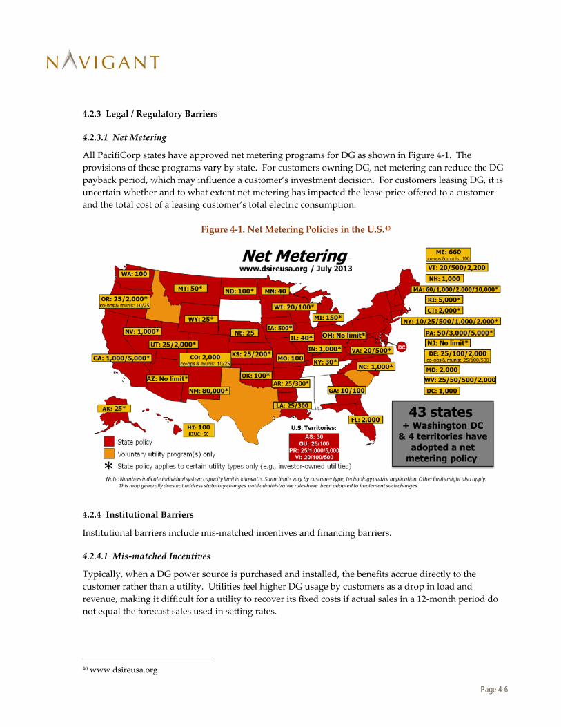
4.2.3 Legal / Regulatory Barriers
4.2.3.1 Net Metering
All PacifiCorp states have approved net metering programs for DG as shown in Figure 4-1. The provisions of these programs vary by state. For customers owning DG, net metering can reduce the DG payback period, which may influence a customer’s investment decision. For customers leasing DG, it is uncertain whether and to what extent net metering has impacted the lease price offered to a customer and the total cost of a leasing customer’s total electric consumption.
Figure 4-1. Net Metering Policies in the U.S.40
4.2.4 Institutional Barriers
Institutional barriers include mis-matched incentives and financing barriers.
4.2.4.1 Mis-matched Incentives
Typically, when a DG power source is purchased and installed, the benefits accrue directly to the customer rather than a utility. Utilities feel higher DG usage by customers as a drop in load and revenue, making it difficult for a utility to recover its fixed costs if actual sales in a 12-month period do not equal the forecast sales used in setting rates.
40 www.dsireusa.org

Page 4-7
4.2.4.2 Financing Barriers
As displayed in Figure 4-2, we are currently enjoying the lowest interest rates available in a generation.
Figure 4-2. US Benchmark Interest Rate41
At some point, these interest rates may rise, significantly increasing the cost of financing DG projects, which typically have high up-front costs and use a loan and/or equity financing to enable projects to proceed. Countervailing this increasing interest rate possibility are trends regarding the risk premium for DG projects. As DG sources get to larger and larger scale from a financing perspective (i.e. deal size and bankability), the risk premium for these projects is likely to go down, especially for newer technologies. In particular, we are seeing solar projects shift from high equity content toward higher loan content, at correspondingly lower interest rates. Current incentives tend to rely on ITC incentives, which require a healthy tax equity market for larger-scale project financing. A recent barrier to larger DG projects occurred when the tax equity appetite shrank dramatically during the recent financial crisis, slowing DG market growth. Congress reacted by creating the Treasury Grant program in response, but this took some time to get set up and operational.
41 http://www.tradingeconomics.com/united-states/interest-rate
Jan/13

Page 5-1
5. Methodology to Develop 2015 IRP DG Penetration Forecasts
5.1 Market Penetration Approach The following five-step process was used to determine the IRP penetration scenarios for DG resources:
1. Assess a Technology’s Technical Potential: Technical potential is the amount of a technology that can physically be installed without taking economics into account.
2. Calculate First Year Simple Payback Period for Each Year of Analysis: From past work in projecting the penetration of new technologies, Navigant has found that Simple Payback Period is the best indicator of uptake. Navigant used all relevant federal, state, and utility incentives in its calculation of paybacks, including their expiration dates.
3. Project Ultimate Adoption Using Payback Acceptance Curves: Payback Acceptance Curves estimate what percentage of a market will ultimately adopt a technology, but do not factor in how long adoption will take.
4. Project Actual Market Penetration Using Market Penetration Curves: Market penetration curves factor in market and technology characteristics to project how long adoption will take.
5. Project Market Penetration under Different Scenarios. In addition to the Base Case scenario, a High Penetration and a Low Penetration case were evaluated that used different 20-year average cost assumptions, performance assumptions, and electricity rate assumptions.
Navigant examined the cost of electricity from the customer perspective, called “levelized cost of energy” (LCOE). A levelized cost of energy calculation takes total installation costs, incentives, annual costs such as maintenance and financing costs, and system energy output, and calculates a net present value $/kWh for electricity which can be compared to current retail prices. A simple payback calculation involves the same analysis conducted for year 1, and calculates the first year costs divided by first year savings to see how long it will take for the investment to pay for itself. Navigant has used LCOE and payback analyses to examine consumer decisions as to whether purchase of distributed resources makes economic sense for these customers, and then projects DG penetration based on these analyses. Each of these five steps is explained below.
5.1.1 Assess Technical Potential
Each technology considered has its own characteristics and data sources that influenced how we assessed technical potential, which is the amount of a technology that can be physically installed within PacifiCorp’s service territory without taking economics into account. We consider each technology in the following subsections.
5.1.1.1 CHP (Reciprocating Engines and Micro-turbines) Technical Potential
CHP technologies can substitute 1:1 for grid power. The technical potential is therefore the amount of power being used by applicable customer classes. In the case of CHP, market studies and our own work has shown that smaller installations are uneconomic, so our technical potential focused on large
Page 5-2
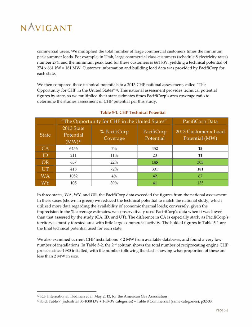
commercial users. We multiplied the total number of large commercial customers times the minimum peak summer loads. For example, in Utah, large commercial class customers (schedule 8 electricity rates) number 274, and the minimum peak load for these customers is 661 kW, yielding a technical potential of 274 x 661 kW = 181 MW. Customer information and building load data was provided by PacifiCorp for each state. We then compared these technical potentials to a 2013 CHP national assessment, called “The Opportunity for CHP in the United States”42. This national assessment provides technical potential figures by state, so we multiplied their state estimates times PacifiCorp’s area coverage ratio to determine the studies assessment of CHP potential per this study.
Table 5-1. CHP Technical Potential
“The Opportunity for CHP in the United States” PacifiCorp Data
State 2013 State Potential (MW)43
% PacifiCorp Coverage
PacifiCorp Potential
2013 Customer x Load Potential (MW)
CA 6456 7% 452 15
ID 211 11% 23 11
OR 657 22% 145 303
UT 418 72% 301 181
WA 1052 4% 42 67
WY 105 39% 41 135 In three states, WA, WY, and OR, the PacifiCorp data exceeded the figures from the national assessment. In these cases (shown in green) we reduced the technical potential to match the national study, which utilized more data regarding the availability of economic thermal loads; conversely, given the imprecision in the % coverage estimates, we conservatively used PacifiCorp’s data when it was lower than that assessed by the study (CA, ID, and UT). The difference in CA is especially stark, as PacifiCorp’s territory is mostly forested area with little large commercial activity. The bolded figures in Table 5-1 are the final technical potential used for each state. We also examined current CHP installations < 2 MW from available databases, and found a very low number of installations. In Table 5-2, the 2nd column shows the total number of reciprocating engine CHP projects since 1980 installed, with the number following the slash showing what proportion of these are less than 2 MW in size.
42 ICF International, Hedman et al, May 2013, for the American Gas Association 43 ibid, Table 7 (industrial 50-1000 kW + 1-5MW categories) + Table 8 Commercial (same categories), p32-33.

Page 5-3
Table 5-2. CHP Install Base
Combined Heat and Power National Database44
State
1980-2013 Reciprocating Engine Installations
(Total / < 2 MW) [in MW]
1980-2013 Micro-turbine Installations
[in MW]
CA 550 / 8.3 34 ID 19 / 3.7 0 OR 48 / 14 .5 UT 42 /4.5 0 WA 21 / 7 .3 WY .5 / .4 .08
Given this very small installation base since 1980 within PacifiCorp’s territory, and summarizing, we conservatively used the minimum CHP technical potential from two sources, PacifiCorp’s customer data, and an area-ratio estimate from a national CHP study.
5.1.1.2 Small Hydro Technical Potential
The detailed national small hydro studies conducted by the Department of Energy in 2004 to 2013, referenced in Section 2.1.5 formed the basis of our estimate of technical potential for small hydro. In the Pacific Northwest Basin, which covers WA, OR, ID, and WY, a very detailed stream by stream analysis was done in 2013, and DOE sent us this data directly. For these states we had detailed GIS PacifiCorp service territory data combined with detailed GIS data on each stream / water source. For each state, we subtracted out the streams that were not in PacifiCorp’s service territory, and summed the technical potentials. For the other two states, Utah and California, we relied on an older 2006 national analysis, and multiplied the given state figures time the area coverage for PacifiCorp within that state that are shown on Table 5-1 above.
44 http://www.eea-inc.com/chpdata. This ICF database is supported by the US Department of Energy and Oak Ridge National Laboratory. It was accessed 6/1/2014.

Page 5-4
Table 5-3. Small Hydro Technical Potential Results
State 2012 Small Hydro Potential (MW)45 CA 32
ID 99
OR 161
UT 62
WA 156
WY 28
5.1.1.3 Photovoltaic Technical Potential
For photovoltaics, a similar approach was taken as the CHP technologies above. We assessed peak load from customer data records provided by PacifiCorp and multiplied by summer peak loads to determine technical potential for each customer class (i.e. rate schedule)46. Rate schedules and customer classes analyzed were chosen according to the following criteria:
1. Rate classes must represent significant revenue
2. Single customer contracts are excluded to preserve confidentiality
3. Partial requirements customers are generally large, over 1 MW, and are qualifying facilities under PURPA and therefore not net-metered customers. They have been excluded.
4. Transmission voltage customers were excluded, as PV projects at these voltage levels are likely to be large-scale PV fields, and exceed the 2 MW net metering limit
We then compared this to the estimated maximum PV array available on the rooftop for an average member of this customer class; the available rooftop area in some cases limited technical potential (for large power users, sometimes sharply). Our assumption is that ground mount system sizes will be larger than the 2 MW net metering limit, and are therefore accounted for elsewhere in the IRP. To estimate maximum available PV array size, we multiplied a number of factors:
• Average rooftop size, derived from PacifiCorp surveys on establishment square feet, divided by an average of two stories
• Assumed PV access factor. Residential tilted rooftops have a 1 in 4 chance of facing south; commercial rooftop access factor is higher as rooftops are flat, but some shading occurs
• Average PV Module Power density (W/Sq Ft). Derived from typical packing factor of 80% (accounting for maintenance footpaths, tilted racking, etc.) and 2013 manufacturer module power specification sheets
45 Note, average hydro technical potential is not likely to change annually 46 Note customer classes were chosen

Page 5-5
An example of this system size calculation is shown for Utah in Table 5-4. Columns 2 through 4 were multiplied together to obtain column 5, and the minimum of the 2013 system size and the summer peak load is the output in the rightmost column.
Table 5-4. PV System Size per Customer Class Example (Utah)
2103 Utah Customer Class (Rate Schedule)
Maximum Available PV Array Size Peak Load
Which One
Chosen
Average floor size
PV Access Factor
2013 average
PV Power density
2013 system
size
2013 Summer
Peak Load
Class System
Size
sf % W/sf kW kW kW Large Commercial (8)
17600 65% 12 137 1112.7 137
Irrigation (10) 17600 65% 12 137 33.9 33.9 Residential (1) 1258 25% 15 4.7 2.8 2.8 Small Commercial (23)
9600 65% 12 75 3.4 3.4
Small Industrial (6) 11464 65% 12 89.4 89.6 89.4 This output column of class system size was then multiplied by the number of customers to obtain technical potential per class. The commercial classes were then summed to show final residential and commercial technical potential for the state of Utah, as shown in Table 5-5.
Table 5-5. Utah PV Technical Potential
2103 Utah Customer Class
(Rate Schedule)
Class System
Size
Number of Customers
Technical Potential per
Class
Commercial / Residential
Technical Potential kW (MW) Total (MW)
Large Commercial (8) 137 274 38
1580 Irrigation (10) 33.9 2784 94 Small Commercial (23) 3.4 82668 282 Small Industrial (6) 89.4 13072 1169
Residential (1) 2.8 740189 2096 2100

Page 5-6
5.1.1.4 Small Wind
For small wind, NREL publishes wind data in GIS format47. An example wind resource map is shown in Figure 5-1. Using PacifiCorp GIS service territory data, we excluded areas in each state outside of its service territory, and then proportionally determined the area within the territory that was Class 4 and above (i.e. the non-green area Figure 5-1 divided by total service area).
Figure 5-1. US Wind Resource Map
These proportions were multiplied by (the customer peak load) times (number of customers) to determine the technical potential for small wind within PacifiCorp’s service territory. A summary of the results is shown in Table 5-6.
47 http://www.nrel.gov/gis/data_wind.html
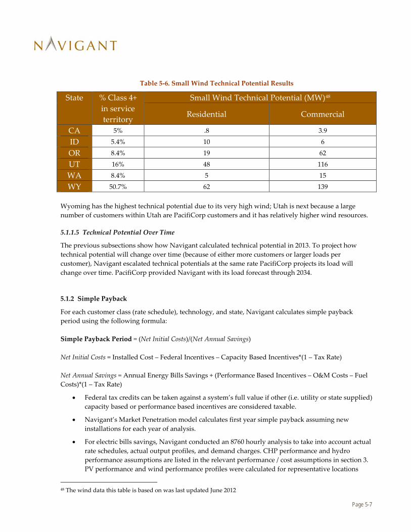
Page 5-7
Table 5-6. Small Wind Technical Potential Results
State % Class 4+ in service territory
Small Wind Technical Potential (MW)48
Residential Commercial
CA 5% .8 3.9
ID 5.4% 10 6
OR 8.4% 19 62
UT 16% 48 116
WA 8.4% 5 15
WY 50.7% 62 139 Wyoming has the highest technical potential due to its very high wind; Utah is next because a large number of customers within Utah are PacifiCorp customers and it has relatively higher wind resources.
5.1.1.5 Technical Potential Over Time
The previous subsections show how Navigant calculated technical potential in 2013. To project how technical potential will change over time (because of either more customers or larger loads per customer), Navigant escalated technical potentials at the same rate PacifiCorp projects its load will change over time. PacifiCorp provided Navigant with its load forecast through 2034.
5.1.2 Simple Payback
For each customer class (rate schedule), technology, and state, Navigant calculates simple payback period using the following formula: Simple Payback Period = (Net Initial Costs)/(Net Annual Savings) Net Initial Costs = Installed Cost – Federal Incentives – Capacity Based Incentives*(1 – Tax Rate) Net Annual Savings = Annual Energy Bills Savings + (Performance Based Incentives – O&M Costs – Fuel Costs)*(1 – Tax Rate)
• Federal tax credits can be taken against a system’s full value if other (i.e. utility or state supplied) capacity based or performance based incentives are considered taxable.
• Navigant’s Market Penetration model calculates first year simple payback assuming new installations for each year of analysis.
• For electric bills savings, Navigant conducted an 8760 hourly analysis to take into account actual rate schedules, actual output profiles, and demand charges. CHP performance and hydro performance assumptions are listed in the relevant performance / cost assumptions in section 3. PV performance and wind performance profiles were calculated for representative locations
48 The wind data this table is based on was last updated June 2012
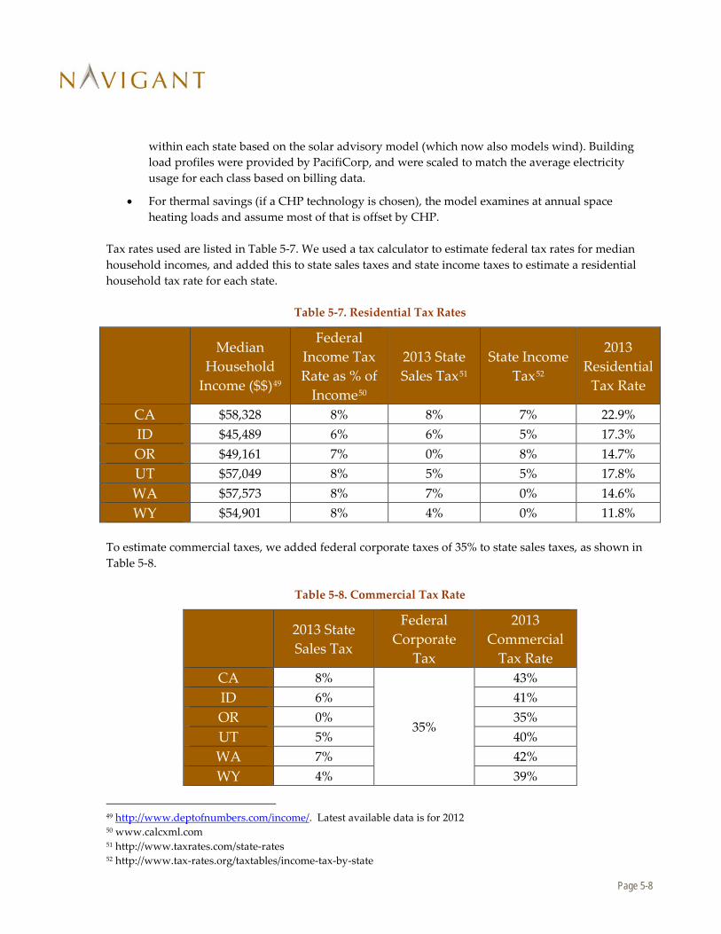
Page 5-8
within each state based on the solar advisory model (which now also models wind). Building load profiles were provided by PacifiCorp, and were scaled to match the average electricity usage for each class based on billing data.
• For thermal savings (if a CHP technology is chosen), the model examines at annual space heating loads and assume most of that is offset by CHP.
Tax rates used are listed in Table 5-7. We used a tax calculator to estimate federal tax rates for median household incomes, and added this to state sales taxes and state income taxes to estimate a residential household tax rate for each state.
Table 5-7. Residential Tax Rates
Median
Household Income ($$)49
Federal Income Tax Rate as % of
Income50
2013 State Sales Tax51
State Income Tax52
2013 Residential
Tax Rate
CA $58,328 8% 8% 7% 22.9% ID $45,489 6% 6% 5% 17.3% OR $49,161 7% 0% 8% 14.7% UT $57,049 8% 5% 5% 17.8% WA $57,573 8% 7% 0% 14.6% WY $54,901 8% 4% 0% 11.8%
To estimate commercial taxes, we added federal corporate taxes of 35% to state sales taxes, as shown in Table 5-8.
Table 5-8. Commercial Tax Rate
2013 State Sales Tax
Federal Corporate
Tax
2013 Commercial
Tax Rate CA 8%
35%
43% ID 6% 41% OR 0% 35% UT 5% 40% WA 7% 42% WY 4% 39%
49 http://www.deptofnumbers.com/income/. Latest available data is for 2012 50 www.calcxml.com 51 http://www.taxrates.com/state-rates 52 http://www.tax-rates.org/taxtables/income-tax-by-state

Page 5-9
5.1.3 Payback Acceptance Curves
For distributed resources, Navigant used the following payback acceptance curves to model market penetration of DG sources from the retail customer perspective:
Figure 5-2. Payback Acceptance Curves
These payback curves are based upon work for various utilities, federal government organizations, and state local organizations. They were developed from customer surveys, mining of historical program data, and industry interviews. Given a calculated payback, the curve predicts what ultimate level of market penetration of the technical potential is likely. For example, if the technical potential is 100MW, a 3 year commercial payback predicts that 15% of this, or 15MW, will be ultimately achieved over the long term.
5.1.4 Market Penetration Curves
To determine the future DG market penetration within PacifiCorp’s territory, the team modeled the growth of DG technologies between now and 2034 for the IRP. The model is a Fisher-Pry-based technology adoption model that calculates the market growth of DG technologies. It uses a lowest-cost approach (to consumers) to develop expected market growth curves based on maximum achievable market penetration and market saturation time, as defined below.53
53 Michelfelder and Morrin, “Overview of New Product Diffusion Sales Forecasting Models” provides a summary of product diffusion models, including Fisher-Pry. Available: law.unh.edu/assets/images/uploads/pages/ipmanagement-new-product-diffusion-sales-forecasting-models.pdf
0%10%20%30%40%50%60%70%80%90%
100%
0 2 4 6 8 10 12 14
Ulti
mat
e Pe
netr
atio
n [%
]
Payback Period (Years)
Residential
Commercial
Industrial
The curves assume 100% adoption is never achieved due to unwillingness to change, mistrust of a new technology, incompatible building designs, etc. This is based upon several prior Navigant examinations of programs.
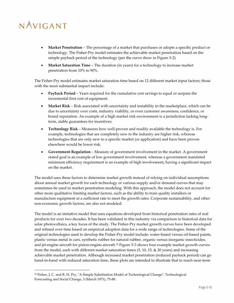
Page 5-10
• Market Penetration – The percentage of a market that purchases or adopts a specific product or technology. The Fisher-Pry model estimates the achievable market penetration based on the simple payback period of the technology (per the curve show in Figure 5-2)
• Market Saturation Time – The duration (in years) for a technology to increase market penetration from 10% to 90%.
The Fisher-Pry model estimates market saturation time based on 12 different market input factors; those with the most substantial impact include:
• Payback Period – Years required for the cumulative cost savings to equal or surpass the incremental first cost of equipment.
• Market Risk – Risk associated with uncertainty and instability in the marketplace, which can be due to uncertainty over costs, industry viability, or even customer awareness, confidence, or brand reputation. An example of a high market risk environment is a jurisdiction lacking long-term, stable guarantees for incentives.
• Technology Risk – Measures how well-proven and readily available the technology is. For example, technologies that are completely new to the industry are higher risk, whereas technologies that are only new to a specific market (or application) and have been proven elsewhere would be lower risk.
• Government Regulation – Measure of government involvement in the market. A government stated goal is an example of low government involvement, whereas a government mandated minimum efficiency requirement is an example of high involvement, having a significant impact on the market.
The model uses these factors to determine market growth instead of relying on individual assumptions about annual market growth for each technology or various supply and/or demand curves that may sometimes be used in market penetration modeling. With this approach, the model does not account for other more qualitative limiting market factors, such as the ability to train quality installers or manufacture equipment at a sufficient rate to meet the growth rates. Corporate sustainability, and other non-economic growth factors, are also not modeled. The model is an imitative model that uses equations developed from historical penetration rates of real products for over two decades. It has been validated in this industry via comparison to historical data for solar photovoltaics, a key focus of the study. The Fisher-Pry market growth curves have been developed and refined over time based on empirical adoption data for a wide range of technologies. Some of the original technologies used to develop the Fisher-Pry model include: water-based versus oil-based paints, plastic versus metal in cars, synthetic rubber for natural rubber, organic versus inorganic insecticides, and jet-engine aircraft for piston-engine aircraft.54 Figure 5-3 shows four example market growth curves from the model, each with different market saturation times (5, 10, 15, & 20 years) and increasing achievable market penetration. Although increased market penetration (reduced payback period) can go hand-in-hand with reduced saturation time, these plots are intended to illustrate that to reach near-term
54 Fisher, J. C. and R. H. Pry, "A Simple Substitution Model of Technological Change", Technological Forecasting and Social Change, 3 (March 1971), 75-88.

Page 5-11
goals, reducing market saturation time is more important than maximizing the long-term achievable market penetration. However, with increased long-term maximum achievable penetration, it may be possible to achieve the same near-term market growth goals with a longer (and less burdensome) market saturation time.
Figure 5-3. Fisher-Pry Market Penetration Dynamics
The market penetration curves used in this study, Navigant assumed that the first year introduction occurred when the simple payback period was less than 25 years (per the payback acceptance curves used, this is the highest payback period that has any adoption. When the above payback period, market risk, technology risk, and government regulation factors above are analyzed, our general Fisher-Pry based method gives rise to the following market penetration curves used in this study:
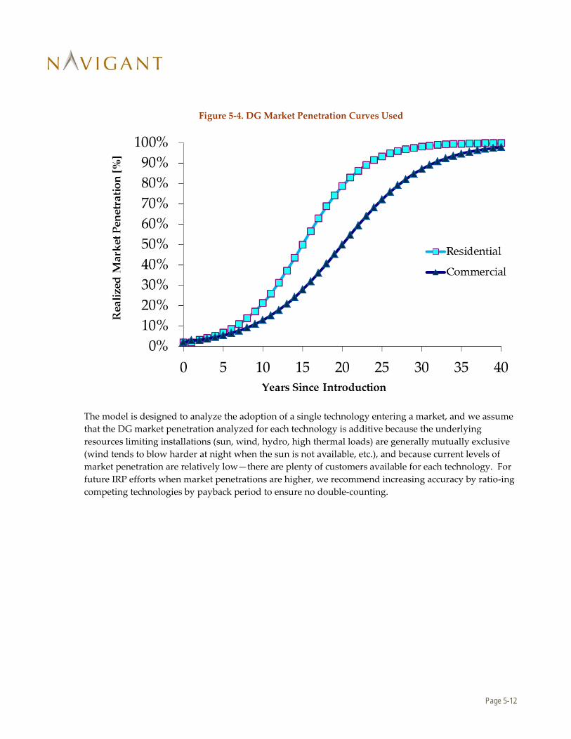
Page 5-12
Figure 5-4. DG Market Penetration Curves Used
The model is designed to analyze the adoption of a single technology entering a market, and we assume that the DG market penetration analyzed for each technology is additive because the underlying resources limiting installations (sun, wind, hydro, high thermal loads) are generally mutually exclusive (wind tends to blow harder at night when the sun is not available, etc.), and because current levels of market penetration are relatively low—there are plenty of customers available for each technology. For future IRP efforts when market penetrations are higher, we recommend increasing accuracy by ratio-ing competing technologies by payback period to ensure no double-counting.

Page 5-13
5.1.5 Scenarios
Navigant analyzed three DG scenarios with its market penetration model, to capture the impact of major changes that could affect market penetration. For the low and high penetration cases, we varied technology costs, performance, and electricity rate assumptions per Table 5-9:
Table 5-9. Scenario Variable Modifications
Scenarios
Technology Costs Performance Electricity Rates
Base Case • See section 3. • As modeled • Inflation rate per IRP
Low DG Penetration
• Hydro (mature): 0%
• PV: 10% lower cost reduction/year
• Other: 5% lower cost reduction/year
• 5% worse • -.5%/year, relative to the base case
High DG Penetration
• Hydro (mature): 2% cost reduction/year
• PV: 10% steeper cost reduction/year
• Other: 5% steeper cost reduction/year
• Reciprocating Engines: 0% better (mature)
• Micro-turbines: 2% better
• Hydro: 5% better (reflecting wide performance distribution uncertainty)
• PV/Wind: 1% better (relatively mature)
• +.5%/year, relative to the base case
The primary driving variable is the amount of cost reduction expected over the next 20 years. Average technology performance assumptions are relatively constant, with a higher variability for hydro as project output is more variable and site specific. Finally, electricity rate changes are modeled in a relatively conservative band, reflecting the long-term stability of electricity rates in the United States. Note that these are all changes to the averages over 20 years, and we expect higher one- year or short term volatility on all of these variables, both up and down. However, when averaged over a long period of time for the 20-year IRP period, long-term trends show this level of variation.

Page 6-1
6. Results
6.1 Technical Potential While technical potential results have been shared for most technologies in the last section, these are summarized by the following graph:
Figure 6-1. Technical Potential Results
As can be seen, the PV (both commercial and residential) technical potential is the highest of all the DG technologies evaluated. Total technical potential is ~10 GW, roughly equivalent to PacifiCorp’s peak summer loads. As indicated in the technical barriers section, it may be difficult for PacifiCorp to incorporate total levels of PV (both DG and large-scale fields) beyond 20-33% without economical energy storage.

Page 6-2
6.2 Overall Scenario Results As shown in Figure 6-2, the near-term ten-year outlook is ~50 MW until 2021, when cost reduction and continued UT/OR incentives significantly improves payback and PV uptake increases dramatically, reaching 900 MW by 2034, the end of the IRP period.
Figure 6-2. Base Case Results
In the low penetration scenario, lower cost reduction than expected results in less short term market penetration, ~ 30 MW; the knee of the higher uptake curve is delayed until 2029 relative to the base case. Over the entire period, penetration is 275 MW by 2034, 60% lower than the base case.
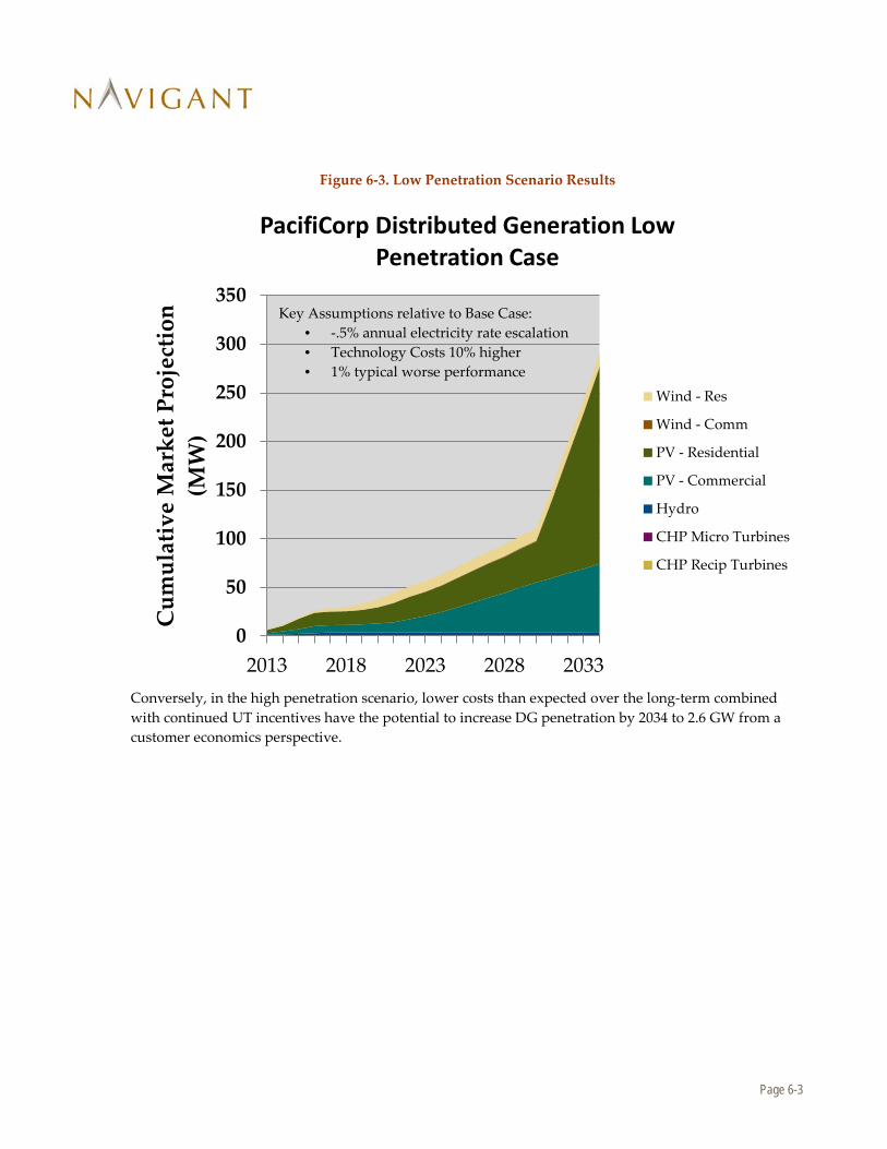
Page 6-3
Figure 6-3. Low Penetration Scenario Results
Conversely, in the high penetration scenario, lower costs than expected over the long-term combined with continued UT incentives have the potential to increase DG penetration by 2034 to 2.6 GW from a customer economics perspective.
0
50
100
150
200
250
300
350
2013 2018 2023 2028 2033
Cum
ulat
ive
Mar
ket P
roje
ctio
n (M
W)
PacifiCorp Distributed Generation Low Penetration Case
Wind - Res
Wind - Comm
PV - Residential
PV - Commercial
Hydro
CHP Micro Turbines
CHP Recip Turbines
Key Assumptions relative to Base Case: • -.5% annual electricity rate escalation • Technology Costs 10% higher • 1% typical worse performance

Page 6-4
Figure 6-4. High Penetration Scenario Results
0
500
1000
1500
2000
2500
3000
2013 2018 2023 2028 2033
Cum
ulat
ive
Mar
ket P
roje
ctio
n (M
W)
PacifiCorp Distributed Generation High Penetration Case
Wind - Res
Wind - Comm
PV - Residential
PV - Commercial
Hydro
CHP Micro Turbines
CHP Recip Turbines
Key Assumptions relative to Base Case: • +.5% electricity rate escalation • Technology Costs 10% lower • 1% typical better performance
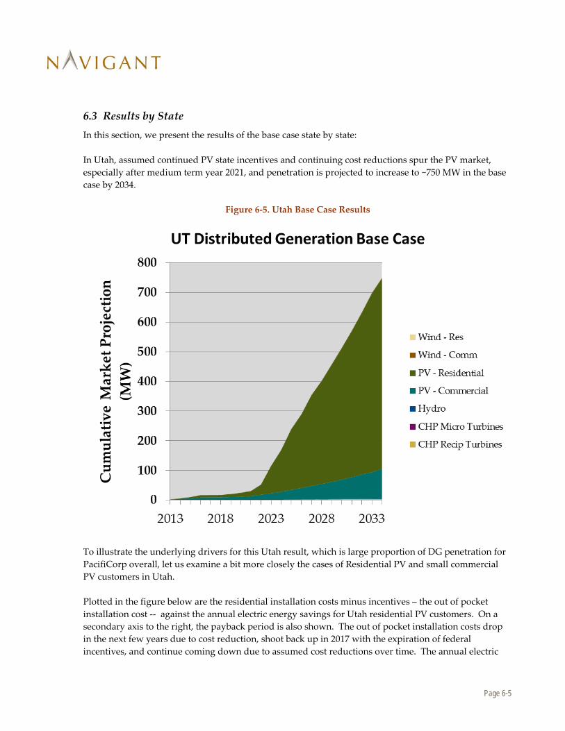
Page 6-5
6.3 Results by State In this section, we present the results of the base case state by state: In Utah, assumed continued PV state incentives and continuing cost reductions spur the PV market, especially after medium term year 2021, and penetration is projected to increase to ~750 MW in the base case by 2034.
Figure 6-5. Utah Base Case Results
To illustrate the underlying drivers for this Utah result, which is large proportion of DG penetration for PacifiCorp overall, let us examine a bit more closely the cases of Residential PV and small commercial PV customers in Utah. Plotted in the figure below are the residential installation costs minus incentives – the out of pocket installation cost -- against the annual electric energy savings for Utah residential PV customers. On a secondary axis to the right, the payback period is also shown. The out of pocket installation costs drop in the next few years due to cost reduction, shoot back up in 2017 with the expiration of federal incentives, and continue coming down due to assumed cost reductions over time. The annual electric
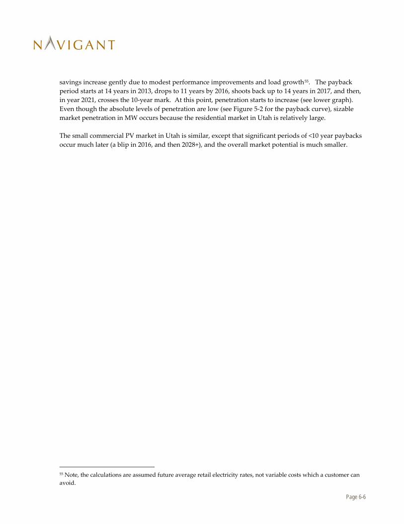
Page 6-6
savings increase gently due to modest performance improvements and load growth55. The payback period starts at 14 years in 2013, drops to 11 years by 2016, shoots back up to 14 years in 2017, and then, in year 2021, crosses the 10-year mark. At this point, penetration starts to increase (see lower graph). Even though the absolute levels of penetration are low (see Figure 5-2 for the payback curve), sizable market penetration in MW occurs because the residential market in Utah is relatively large. The small commercial PV market in Utah is similar, except that significant periods of <10 year paybacks occur much later (a blip in 2016, and then 2028+), and the overall market potential is much smaller.
55 Note, the calculations are assumed future average retail electricity rates, not variable costs which a customer can avoid.
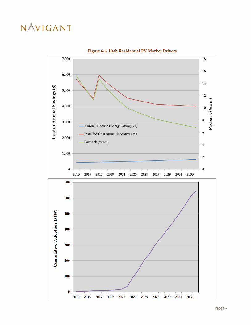
Page 6-7
Figure 6-6. Utah Residential PV Market Drivers

Page 6-8
Figure 6-7. Utah Small Commercial PV Market Drivers
Varying incentive level jogs
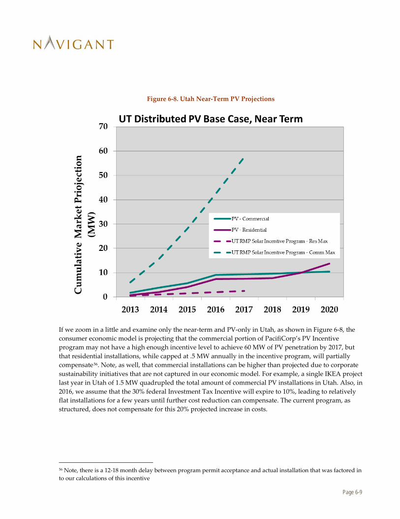
Page 6-9
Figure 6-8. Utah Near-Term PV Projections
If we zoom in a little and examine only the near-term and PV-only in Utah, as shown in Figure 6-8, the consumer economic model is projecting that the commercial portion of PacifiCorp’s PV Incentive program may not have a high enough incentive level to achieve 60 MW of PV penetration by 2017, but that residential installations, while capped at .5 MW annually in the incentive program, will partially compensate56. Note, as well, that commercial installations can be higher than projected due to corporate sustainability initiatives that are not captured in our economic model. For example, a single IKEA project last year in Utah of 1.5 MW quadrupled the total amount of commercial PV installations in Utah. Also, in 2016, we assume that the 30% federal Investment Tax Incentive will expire to 10%, leading to relatively flat installations for a few years until further cost reduction can compensate. The current program, as structured, does not compensate for this 20% projected increase in costs.
56 Note, there is a 12-18 month delay between program permit acceptance and actual installation that was factored in to our calculations of this incentive
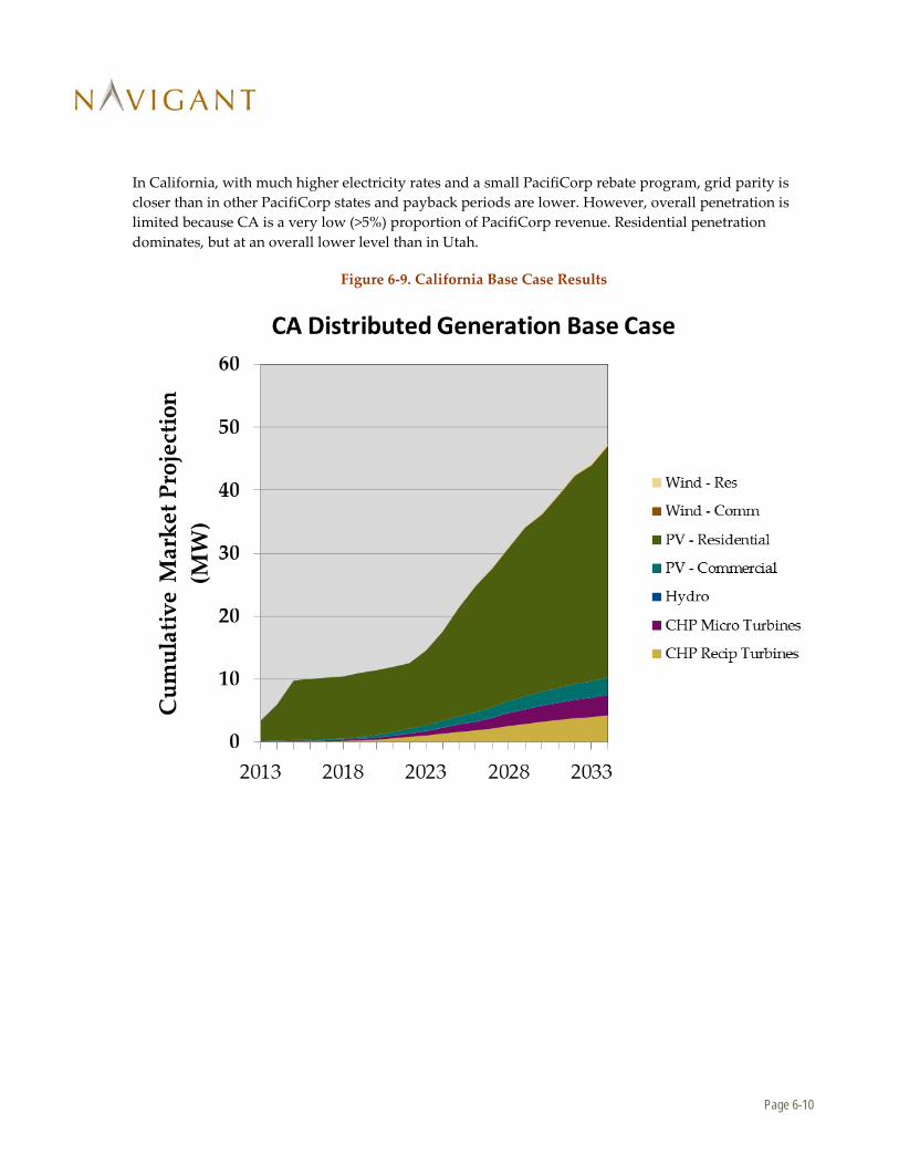
Page 6-10
In California, with much higher electricity rates and a small PacifiCorp rebate program, grid parity is closer than in other PacifiCorp states and payback periods are lower. However, overall penetration is limited because CA is a very low (>5%) proportion of PacifiCorp revenue. Residential penetration dominates, but at an overall lower level than in Utah.
Figure 6-9. California Base Case Results
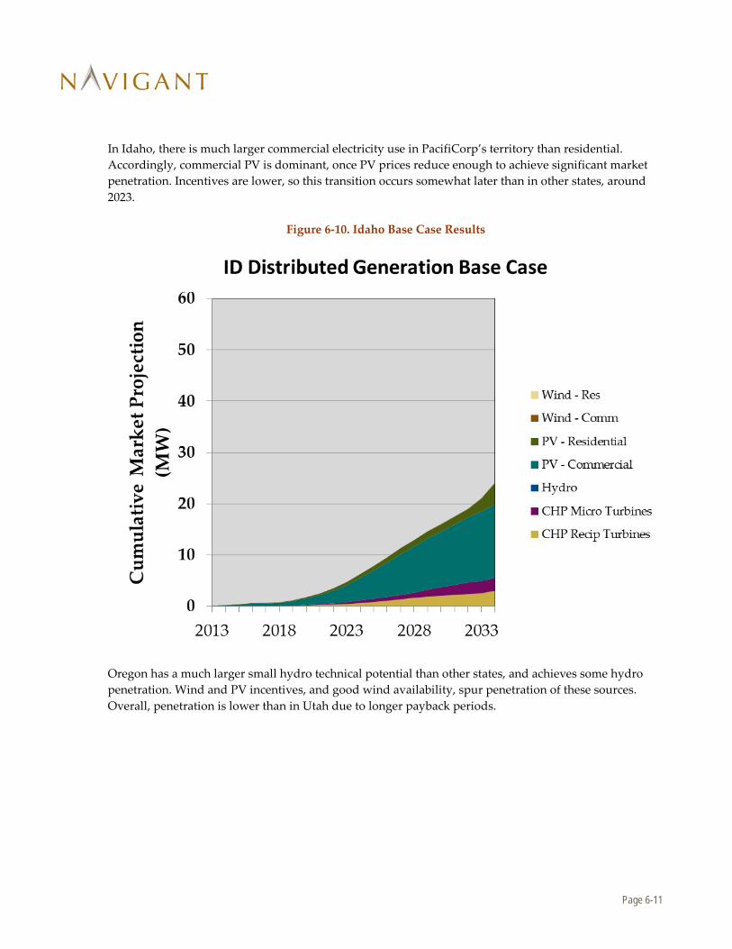
Page 6-11
In Idaho, there is much larger commercial electricity use in PacifiCorp’s territory than residential. Accordingly, commercial PV is dominant, once PV prices reduce enough to achieve significant market penetration. Incentives are lower, so this transition occurs somewhat later than in other states, around 2023.
Figure 6-10. Idaho Base Case Results
Oregon has a much larger small hydro technical potential than other states, and achieves some hydro penetration. Wind and PV incentives, and good wind availability, spur penetration of these sources. Overall, penetration is lower than in Utah due to longer payback periods.

Page 6-12
Figure 6-11. Oregon Base Case Results

Page 6-13
Washington, with a relatively small PacifiCorp area, and rates that are somewhat lower, is projected to achieve up to 10 MW by 2034 in the base case.
Figure 6-12. Washington Base Case Results
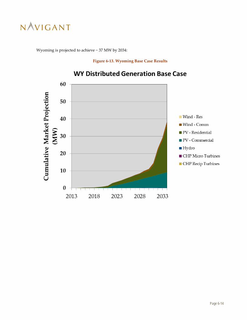
Page 6-14
Wyoming is projected to achieve ~ 37 MW by 2034:
Figure 6-13. Wyoming Base Case Results

Page 6-15
6.4 Results by Technology Each technology is shown in turn. Non-construction and non-standby power reciprocating engines will mostly occur in OR, CA, ID, and UT. Negligible penetration is projected for WY and WA57.
Figure 6-14. Reciprocating Engines Base Case Results
57 Hence these are not showing as series in Figure 36.
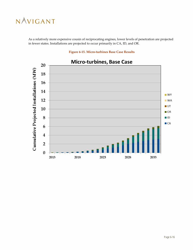
Page 6-16
As a relatively more expensive cousin of reciprocating engines, lower levels of penetration are projected in fewer states. Installations are projected to occur primarily in CA, ID, and OR.
Figure 6-15. Micro-turbines Base Case Results

Page 6-17
Small levels of small hydro penetration are likely to occur in some states -- WY, WA, UT, and OR. WA, and UT have higher technical potential, leading to slightly more penetration; Oregon, with the highest technical potential, achieves ~5 MW of penetration when current incentives expire in 2017, with little penetration thereafter.
Figure 6-16. Small Hydro Base Case Results

Page 6-18
Due to higher residential electricity rates, and therefore lower payback periods, residential installations dominate PV projections, especially after 2022.
Figure 6-17. Photovoltaics Base Case Results

Page 6-19
As shown below and in the Utah results above, most of this dramatic residential growth after 2022 is projected to occur in Utah, with continued incentives and continued cost reduction lowering payback residential payback periods.
Figure 6-18. Photovoltaics Residential Base Case Results

Page 6-20
Commercial PV projections are much lower. Utah dominates due to higher incentives and its relatively large proportion of technical potential.
Figure 6-19. Photovoltaic Commercial Base Case Results

Page 6-21
Residential small wind installations are projected to be more economic than commercial:
Figure 6-20. Small Wind Base Case Results

Page 6-22
These are dominated by Oregon market penetration, which occurs largely due to an incentive that is projected to phase out by 2021.
Figure 6-21. Small Wind Residential Results
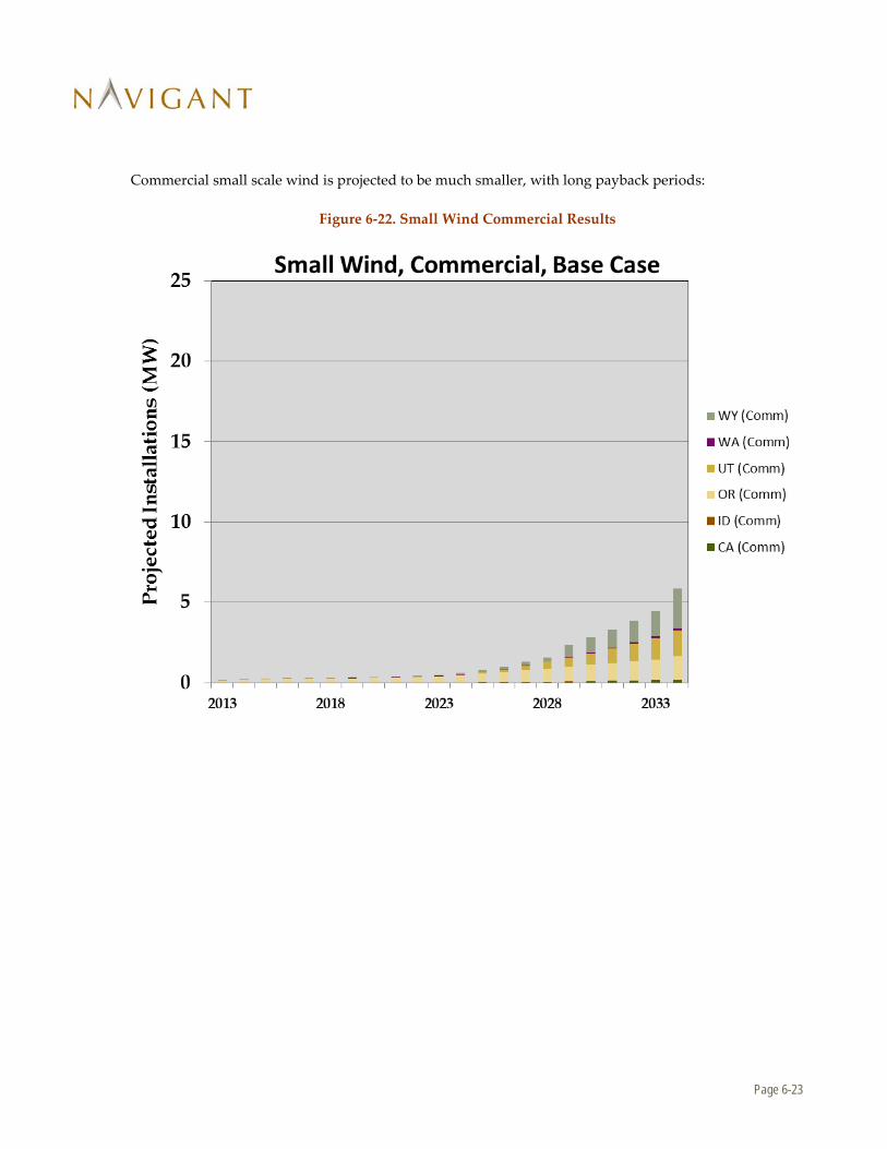
Page 6-23
Commercial small scale wind is projected to be much smaller, with long payback periods:
Figure 6-22. Small Wind Commercial Results

Page A-1
Appendix A. Glossary
$/WpDC -- $/ peak watt DC. Solar modules produce DC power which is then converted to AC by an inverter
CHP – Combined Heat and Power
DG - Distributed Generation – electricity sources that are purchased by the consumer
HAWT – Horizontal-axis wind turbine
IRP – Integrated Resource Plan
ITC – Investment Tax Credit
LCOE – Levelized Cost of Energy, a measure of the cost of electricity in $/kWh
MW – Mega-watt, a measure of power
Net Meter – a regulation which allows the customer to feed excess power generated back into the grid
O&M – Operations and Maintenance costs
PV – Photovoltaic, or Solar, or Solar Electric (used interchangeably). A technology that generates electricity when a module is exposed to sunlight.
PV Array – multiple PV modules grouped together to generate power
PV Module – a 1-2 m2 solar component that can be readily handled by 1-2 people which generates DC electricity (like a battery)
SWT – Small Wind Turbine
Solar Electric – Photovoltaic
Solar Thermal – an alternative PV technology which concentrates solar energy to raise the temperature of a heat transfer fluid
VAWT – Vertical-axis wind turbine

Page B-2
Appendix B. Summary Table of Results
Base Case (MW Projected) 2015 2020 2025 2030
CA 9.8 11.4 21.5 36.3 ID 0.4 1.8 7.9 16.0 OR 5.3 15.5 24.0 36.7 UT 9.9 24.7 239.3 513.4 WA 0.1 0.4 2.6 6.1 WY 0.2 0.9 5.6 11.1
Low Penetration Case (MW) 2015 2020 2025 2030
CA 8.0 8.8 10.1 12.3 ID 0.3 0.9 3.3 6.1 OR 3.9 12.6 17.2 21.2 UT 6.9 14.9 38.1 64.1 WA 0.0 0.2 0.9 1.9 WY 0.1 0.5 1.5 4.8
High Penetration Case (MW) 2015 2020 2025 2030
CA 12.2 14.7 45.7 74.8 ID 0.6 3.5 22.8 68.5 OR 6.6 19.9 43.0 99.5 UT 16.0 143.2 729.0 1347.2 WA 0.2 1.3 7.6 28.8 WY 0.3 3.1 42.1 109.4