Divergent Inflation in Euroland A Phillips Curve approach to the EMU-12

Master thesis within Economics

Author: Anders Nilsson

Tutor: Ph.D Sara Johansson

Ass. tutor: Ph.D Candidate Peter Warda

Jönköping, June 2011

Master Thesis in Economics

Title: Divergent Inflation in Euroland – A Phillips Curve Approach to the EMU-12

Author: Anders Nilsson

Tutor: Ph.D Sara Johansson

Ass. tutor Ph.D Candidate Peter Warda

Date: [2011-06-10]

Subject terms: EMU, euro, Optimum Currency Area, Phillips Curve

Abstract

This thesis investigates the cause and implications of the divergent inflation rates of the EMU-12 countries between the years 1998 and 2010. The EMU and the euro are put into a context with the classic theory of Optimum Cur-rency Area, where the economic benefits and cost of joining a monetary union is reviewed. The inflation divergence in the euro area is then described and in-vestigated. Empirically, a Phillips Curve model is constructed in order to de-termine if the EMU-12 nations’ inflation rates are equally sensitive to changes in unemployment as the EMU average. This is done using a Panel Least Square estimation for the EMU-12. Each nation is then tested separately against the EMU average. The result provides evidence that the EMU-12 nations’ inflation rates are not equally sensitive to changes in unemployment as the EMU aver-age. The result is negative for the EMU-12 in an Optimum Currency Area con-text. Given the results, the EMU-12 cannot be considered to be an Optimum Currency Area, at least not yet.

i

Aknowledgements

I would like to start by thanking my two supervisors Sara Johansson and Peter Warda for their help and guidence through the process of this thesis. A special thanks is due for Peter who effortless helped to minimize my grammar mistakes. I would also like to thank my friends and classmates for the support over this period. Finally, I thank the discussant Cindy, who pointed out a few flaws and suggested improvements of the text.

ii

Table of Contents

1 Introduction .......................................................................... 1

2 Theoretical Framework ........................................................ 3

2.1 Optimum Currency Area ................................................................ 3

2.1.1 Advantages and Disadvantages ......................................... 3

2.1.2 Labor Mobility ..................................................................... 5

2.1.3 Endogeneity of a Currency Area ......................................... 6

2.2 Inflation and Unemployment .......................................................... 7

2.3 Monetary Policy ............................................................................. 9

3 Inflation in the EMU-12 ....................................................... 11

3.1 Inflation Divergence ..................................................................... 11

3.1.1 Price Convergence ........................................................... 12

3.1.2 Economic Transmission .................................................... 13

3.1.3 Exchange Rate Volatility ................................................... 15

3.2 Implications of Inflation Divergence ............................................. 16

4 Empirical Investigation ...................................................... 19

4.1 Model .......................................................................................... 19

4.2 Data ............................................................................................. 22

4.3 Descriptive Statistics ................................................................... 22

4.4 Results ........................................................................................ 24

5 Summary and Conclusions ............................................... 28

List of references ..................................................................... 29

iii

Figures Figure 2-1: Short-run Phillips Curve ............................................................... 8

Figure 2-2: Augmented Phillips Curve ............................................................ 8

Figure 3-1: Annual HICP for the EMU-12 ..................................................... 11

Figure 3-2: Quarterly HICP Q1 1997-Q4 2010 ............................................. 12

Figure 3-3: Quarterly HICP Q1 1997-Q4 2010 ............................................. 12

Figure 3-4: USD-EUR Exchange Rate ......................................................... 16

Figure 4-1: HUR Quarterly 1998-Q2 - 2010-Q3 ........................................... 21

Figure 4-2: ���,�, grouped together by country on the horizontal axis ............ 23

Figure 4-3: ���,� grouped together by country on the horizontal axis ............. 23

Tables Table 3-1: Central Government Debt % of GDP .......................................... 14

Table 3-2: Annual changes in HICP ............................................................. 14

Table 4-1: Descriptive Statistics, ���,� and ���,� ............................................... 22

Table 4-2: Panel Least Square fixed effect model estimations..................... 24

Table 4-3: Estimation of equation (4.7), country specific model ................... 26

Appendix Appendix A - Quarterly HICP for the EMU-12 ............................................... 33 Appendix B - Residual Diagnostics ................................................................ 35 Appendix C - Hausman Test ......................................................................... 37 Appendix D - Diagnostic Tests for Equation (4.7) ......................................... 38

1

1 Introduction

This year forms the 12 year anniversary since the formation of the euro. During this period the monetary union has expanded from 11 member countries to the 17 members it holds today. Estonia became the most recent nation to join the EMU on the 1st of January 2011. The creation of the monetary union within the European Union (EU) may be the most ambitious natural economic experiment ever undertaken and researchers have been highly interested in its effects (De Nardis and Vicarelli, 2003). After the fixed exchange rate me-chanism (ERM) broke down in 1992, it became evident that a system of fixed exchange rates was not stable enough to eliminate exchange rate volatility in the long-run. If ex-change rate volatility was going to be eliminated, a more stable system was required. In or-der to establish such a system, a single currency was necessary (Gerber, 2011).

The idea to form monetary unions is not new, Nobel laureate Robert Mundell is generally considered as the “father” of the Optimum Currency Area (OCA) theory with his seminal article published 50 years ago (Mundell, 1961). Although Mundell emphasized mobility of production factors (i.e. capital and labor) as a probable boundary for Western Europe to be considered as an OCA, the research today focus on other properties and complete factor mobility is not generally seen as a prerequisite for the formation of a monetary union (Rose, 2008). Today, focus lies on economic and political integration, the degree of symme-tric business cycles, the effects of a common currency on trade and wage and price flexibili-ty (Mongelli, 2005). This thesis focuses on asymmetric inflation rate movements.

The purpose of this paper is to investigate if changes in unemployment for the EMU-121 affect the inflation rate similar to the EMU average. The paper will contribute to the EMU and OCA literature and give clarity if the EMU-12 nations are similar enough to the EMU average to potentially constitute of an OCA. Put differently, the aim is to investigate if there is a significant difference in inflation rate sensitivity to changes in unemployment across the EMU-12. This is an important topic since most previous research only have fo-cused on investigating if business cycles are symmetric in the euro area, not the effects of symmetric cycles. My thesis goes one step further and opens for the possibility that even if business cycles are symmetric, they may have asymmetric effects. If this is the case, the EMU-12 cannot be considered as an OCA since the policy constructed by the ECB cannot be optimal for all nations. The study make use of panel data of Harmonized Index of Con-sumer Prices (HICP) and Harmonized Unemployment Rates (HUR) between 1998 and 2010 to estimate a model that is set up to capture any effect that unemployment changes have on inflation rate changes, which is compared to the EMU average. The goal is to be able to conclude if the inflation rates have similar sensitivity across the EMU-12 nations. This will be important in order for the European Central Bank (ECB) to conduct a one-size monetary policy that is suitable for each of the EMU-12 countries.

The hypothesis is formulated as follows. If the national inflation rate movement differ sig-nificantly from the EMU average, managed by the ECB, it is not possible for the ECB to perform a suitable monetary policy for the particular nation in question. Therefore, the country could face considerable real costs since they would be, in a way, “stuck” with a monetary policy not suited for them. It follows that a “one-size-fits-all” monetary policy has the potential to work well in one country, while for another country the same policy might be too expansionary and for a third nation at the same time be too restrictive. For a

1 EMU-12: Austria, Belgium, Finland, France, Germany, Ireland, Italy, Luxemburg, Netherlands, Portugal,

Spain and Greece, who joined in 2001.

2

country with a divergent inflation rate, the costs for giving up its ability to fine tune mone-tary policy could potentially become so high that it outweighs all gains from a common currency. In addition, since the EMU-12 has been using the euro for over 10 years and the convergence mechanism has been in place since the early 1990’s, one should suspect that any natural inflation differences from price and market convergence should have been ac-complished already. We would expect that a long-run equilibrium should have been reached by now, at least for the EMU-12.

The thesis is outlined as followed: The next chapter reviews the current literature on OCA and discusses the potential advantages and disadvantages of currency unions. In addition, it also provides a quick review of the relationship between unemployment and inflation. Chapters 3 closely examine the potential causes of inflation differences and consider the arising implications, as well as the characteristics of inflation rates of the EMU-12. Chapter 4 presents the empirical analysis and its results. The last section summarizes and concludes the thesis.

3

2 Theoretical Framework

2.1 Optimum Currency Area

The theory on OCA has a long history and has stood the test of time well, recently the cre-ation of the EMU has obtained much interest of researchers, as well as mine. De Nardis and Vicarelli (2003) refer to the EMU as the most ambitious experiment in creating a cur-rency union ever undertaken. Chapter 2 will review the theoretical background of OCA theory in a modern setting with a focus on the euro. The discussion begins with a short de-finition and introduction to OCA theory.

An OCA is defined as a geographical area where the benefits of sovereign currencies are low and the benefits from a common currency are higher for the particular region. The common currency will be a better absorber to external shocks and reduce the effects of shocks more efficient than a system of sovereign currencies (Mongelli, 2005). This will be achieved if the economies that are members of the monetary union fulfill certain criteria’s or prerequisites. The classic prerequisite is mobility of production factors, capital and labor. Where the mobile labor and capital works to offset any asymmetric shock in the area in or-der to distribute any asymmetric effect evenly across the region (Mundell, 1961). More re-cent factors include symmetry of business cycles, the extent of trade and similarities of economic structures. These reasons are important since the members of a monetary union need to react in the same way to external shocks for the common currency to be efficient. In fact, recently the argument has been made that the introduction of a common currency, by itself, helps to achieve these properties or prerequisites (Mongelli, 2005; Frankel and Rose, 1998).

2.1.1 Advantages and Disadvantages

Why should a country give up its ability to conduct an independent monetary policy and its monetary sovereignty, in other words, why join the EMU?

Various reasons come to mind and it is important to remember that they vary for any indi-vidual nation. Even when all possible economic pros and cons have been examined there might still be important political and historical reasons that are different for individual na-tions in Europe. It is important to note that political reasons for joining the EMU might make it rational to join even if economic benefits are low. However, I will not elaborate or investigate any political or psychological factors further in this thesis, the focus is on eco-nomics2. Baldwin (2006) notes that politics, not economics, was highly important in the creation of the euro and Artis (2003) writes that political aspects are relevant as well as economics for example.

There is no functional framework or measurable tests to analyze if a set of nations consti-tute an OCA and would benefit from a common currency (Mongelli 2005). Although text-books refer to a couple of diagrams and schedules as ways to compare costs and benefits they remain analytical tools with no measurable way of quantifying any potential cost or benefit (Artis, 2003; Krugman and Obstfeld, 2006). In addition, the textbook approach of-fers some hints but no clear answer if the euro zone qualifies as an OCA. The analysis giv-

2 Such factors could include the possibility of increased political influence and additional allies as a positive ef-

fect and loss of a strong national symbol for sovereignty as negative. Even the simplicity of not having to buy foreign currency and calculate prices when on vacation is likely a positive reason from an individual perspective.

4

en often suggests that some countries, but not all of the original euro members, might be considered as part of an OCA. Some indicators provide positive results while other sug-gests a less positive outlook. Generally the conclusion, if explicitly given, is negative, the euro area is not believed to be an OCA (McDowell, 2006; Krugman and Obstfeld, 2006).

The cost of adopting the euro is simple from an economic perspective, it occurs at the ma-cro level. When adopting a common currency a country effectively gives up its ability to tai-lor monetary policy at the national level (De Nardis and Vicarelli, 2003; Frankel and Rose, 1998 among others). In addition, national exchange rate fluctuations cannot work as auto-matic stabilizers in the event of a recession or an economic boom (Feldstein, 1997). These implications are different for individual nations since a country’s relative economic size af-fects its ability to influence the world market, hence, to maintain an effective monetary pol-icy. If a small country is using a sovereign currency it is potentially putting itself at risk as smaller currencies and economies, all else equal, provide a more risky environment and in-creased uncertainty for investments. Therefore, the macroeconomic benefit of an indepen-dent monetary policy might be low, even irrelevant for small countries. These are reasons for why small economies like Luxembourg, Monaco and Lichtenstein shared a common currency with more stable nations before the creation of the euro, they were simply too small. Therefore adopting a more widely used currency, the dollar or euro, creates in-creased credibility for small nations (Baldwin, 2006).

A fixed exchange rate regime effectively eliminates any exchange rate fluctuation and there-fore removes any foreign exchange rate uncertainty. A common currency creates deeper in-tegration between countries and regions. It irrevocably removes exchange rates so they cannot be devalued or floated in the future (De Nardis and Vicarelli, 2003). More impor-tantly, it creates a unified market where all prices are denominated in the same nominal value, which effectively creates full transparency and eliminates any cost of hedging or for-eign exchange rate costs inside the currency area. These costs are likely to be specifically important for smaller firms that cannot benefit from departments devoted to hedging and exchange rate risk (De Nardis and Vicarelli, 2003). Through this mechanism, members of a currency union are expected to experience more economic integration through increased trade between members. In fact, international trade within the currency union would be transformed into what used to resemble domestic trade (De Nardis et al. 2008). Therefore, it will create better efficiency through increasing competition and price comparison which in turn will lead to more specialization across regions and more efficient use of resources and factors of production (Mongelli, 2005; Micco et al., 2003; Shiavo, 2008). In short, trade theory expect that trade increases utility, therefore since a currency union is assumed to in-crease trade, subsequently it will increase utility (or consumption) of its population (Krug-man and Obstfeld, 2006). Moreover, an increase in trade between countries would increase any political integration between countries, which in turn could lead to further global inte-gration and eventually more peace and stability (Rose, 2000). So the benefits might be ex-tremely large, although difficult to measure and highly hypothetical in some cases. Fur-thermore, benefits of greater stability and peace might only show its true colors in the very long-run, and even then a counterfactual would not exist for comparison.

Several studies have been conducted on currency unions effect on increased trade, the re-sults differ but has since the contribution from Rose (2000) been scaled down and revised from a 200 percent increase to much lower estimates. Rose and Stanley (2005) estimate an effect of 30-90 percent. Others argue that the euro effect is likely to be much lower, how-ever the estimates are uncertain and change significantly when methods and data are al-tered. De Nardis et al. (2008) find a 4 percent increase and estimate a long-run effect of 17

5

percent. Baldwin (2006) finds an increase in intra-euro trade at 5-10 percent and Havranek (2010), who introduce a trend parameter for increased economic integration, finds no posi-tive effect at all. In the end it seems like the euro have had positive effects on trade, both inside and outside the euro area, however its magnitude remains uncertain3.

Although the creation of the euro is likely to have increased trade between its members, it is likely not to have been caused by a loss of transaction costs and exchange rate volatility (Baldwin, 2006). Instead Baldwin (2006) suggests that the increased trade is likely to have been caused by a reduction of the fixed-cost of introducing a new-good to the euro market. This would induce that the benefit from eliminating any cost of currency conversion and exchange rate risk is small, if not even negligible in the aggregate.

To summarize, the more important benefits include increased trade, efficient allocation of resources, increased political integration and, for small economies, increased credibility. The costs are associated with the loss of an independent monetary policy. Of course these potential costs and benefits will all be different in any particular nation, therefore any policy suggestion in favor of or against the euro is, in general, not possible to make.

2.1.2 Labor Mobility

Since the influential and regularly cited contribution by Mundell (1961) the theory concern-ing OCA has been revised, new ideas have been added and any prerequisites for forming a monetary union is less clear today. There was however no clear test or theory suggested at first, although Mundell (1961) emphasized on labor mobility to offset any asymmetric shocks within a monetary union. In recent literature this criteria has been scaled down (Rose, 2008). Labor is not mobile in the short-run and cannot therefore act as a stabilizing mechanism other than in the long-run, where mobility becomes important in order to achieve low unemployment (Mongelli, 2005). In addition, it is noted that labor is far less mobile in Europe than in the U.S. and although borders pose no barrier for labor mobility inside the EU (Arrests et al. 2001), culture and language are at present more severe barriers for mobility, factors not present in the U.S. (Martin, 2001; Mongelli, 2005). Moreover, Mongelli (2005) writes that wage flexibility is low in Europe and that different labor market institutions including collective wage bargaining, unemployment insurance and protection increase the rigid structure of wages. Huber (2004) concludes that unemployment protec-tion is an important reason for low labor migration within Europe.

Since it has clearly been proven that labor is not mobile in the short-run it is unlikely that labor mobility would be sufficient to eliminate (any) country specific or asymmetric shocks in a short-run perspective. It is therefore stressed that for a monetary union to be success-ful, regions (countries) across the union need to experience symmetric business cycles. In-creased economic integration, similarities in business cycles, increased trade flows and ho-mogenous markets for goods and services would make it unnecessary for labor mobility to offset any asymmetric shocks. In a completely homogenous market, business cycles would be symmetric and there is no need for a mobile labor market to offset any asymmetric shocks (Rose, 2008).

For an unemployed worker the situation would be approximately equal across all regions. The only possibility would not be to move to another region, but instead move to another industry or sector, which, given that the need to acquire new education, is in most cases not viable in the short-run either, given that re-training and searching takes time (Mongelli,

3 For a good overview see De Nardis et al. (2008).

6

2005). However, this is not a problem specific for currency unions, this is a general prob-lem of business cycles and labor markets (Rose, 2008). A flexible labor market is of course better than a rigid one. Hence, to increase labor movement and flexibility within the EU and the EMU area is still an important goal to strive for, perhaps not necessary for the suc-cess of the euro but for a more functional labor market within the EU (Artis, 2003). Melitz (2004) also promotes a flexible labor market before a more rigid one. One policy within the EU that aims to improve workers flexibility is the Erasmus Exchange program. It encou-rages university students to study abroad within the EU via scholarships. If students find it natural to study in any European country they would be more flexible in their decision of where to live and work, they will also expand their personal network and establish friends all over the continent. Hence, in the long-run a more flexible workforce might enter the la-bor market.

2.1.3 Endogeneity of a Currency Area

The “endogeneity argument” of currency unions was first presented by Frankel and Rose (1998) who introduced the link between trade patterns and business cycles. Their study concludes that regions that trade extensively with each other experience more similar busi-ness cycles. The idea is as follows: even though a country does not fulfill the criteria for joining a currency union, it will, through convergence and increase economic integration, fulfill the necessary criteria for an OCA after a common currency has been implemented. Therefore, the actual introduction of a single currency helps the monetary union to achieve optimality and fulfilling the various criteria for OCA. Thus, making a monetary union justi-fiable ex post, rather than ex ante (Frankel and Rose, 1998). Artis (2003) expresses the argu-ment such that the reason for idiosyncratic shocks simply is idiosyncratic policy, therefore the best solution to achieve optimality is just to implement a single currency and a single monetary policy.

This is a viable argument, however one needs to be careful and remember that such con-vergence will not appear automatically. For the EMU this has been carefully done through several years of economic collaboration and unification policies, not just for the EMU countries but for the whole EU this is a common goal. For example, the Single Market Program introduced in 1993 was aimed at increasing competition and transparency in the market for goods and services (Baddinger, 2007). In addition the Maastricht Treaty pro-vided countries with explicit criteria that were to be fulfilled prior to joining the EMU (Krugman and Obstfeld, 2006). The shape of the endogeneity argument makes it a self ful-filling prophecy where it seems like all will be well with time. Needless to say, reality is not this simple. Even though an endogeneity argument is definitely plausible, it has been de-bated. The most profound argument against endogeneity is that since the endogeneity ad-vocators argue that more integration lead to more trade and a better integrated market, it will also lead to a higher degree of regional specialization. If regions become highly specia-lized with differentiated production, they are likely to face uncorrelated fluctuations in de-mand. Hence, a more integrated market and regional specialization do not lead to a homo-genous market with symmetric business cycles, it could lead to the exact opposite since re-gions will be affected differently to industry specific demand shocks (De Grauwe and Mongelli, 2005; Melitz, 2004). Recent authors have however contributed with positive signs of endogeneity, such as Schiavo (2008) who presents some evidence of the endogeneity hypothesis, De Grauwe and Mongelli (2005) provide a short summary of the endogeneity vs. specialization argument and conclude that so far, increased integration has lead to more symmetry and less country specialization rather than the opposite.

7

Even though a problem with increased specialization could lead to idiosyncratic business cycles, integration and efficient capital markets could potentially solve such problems with investors from different regions keeping holdings on each other. The idea is for example put forward by McKinnon (2004), Mongelli (2005) and Martin (2001), who argue that deep financial integration would insure regions who experience asymmetric shocks, thus helping to improve efficiency of an EMU wide capital market. The idea is also shared by Artis (2003) who believes that such a system would mitigate any asymmetric shocks. Therefore, a regional demand shock would through an efficient capital market affect the whole currency area, not just the single region. Kalemli-Ozcan et al. (2003) test the theory and find evi-dence that risk sharing and industrial specialization is positively related. Moreover, if the argument is correct, symmetric business cycles would no longer constitute as a prerequisite for an OCA (Martin, 2001).

There is also controversy in what direction any causality of endogeneity flows. Do currency unions stimulate economic integration, or are currency unions an evolution of increased economic integration (Rose and Engel, 2002)? There is no way to determine the actual di-rection of causality, logically this is likely to be individual for the monetary union in ques-tion and it is likely to be a mix of both causality directions. That is, there is probably some economic integration (e.g. trade) between nations considering a common currency, why else adopt a single currency? However, after an introduction there is no reason to believe that economic integration would decline, most likely the formation of a currency union will lead to positive economic effects, all else equal. In their paper, De Grauwe and Mongelli (2005) conclude that there has been convergence of prices in the goods market, however they are unable to determine if this convergence is caused explicitly by the EMU.

2.2 Inflation and Unemployment

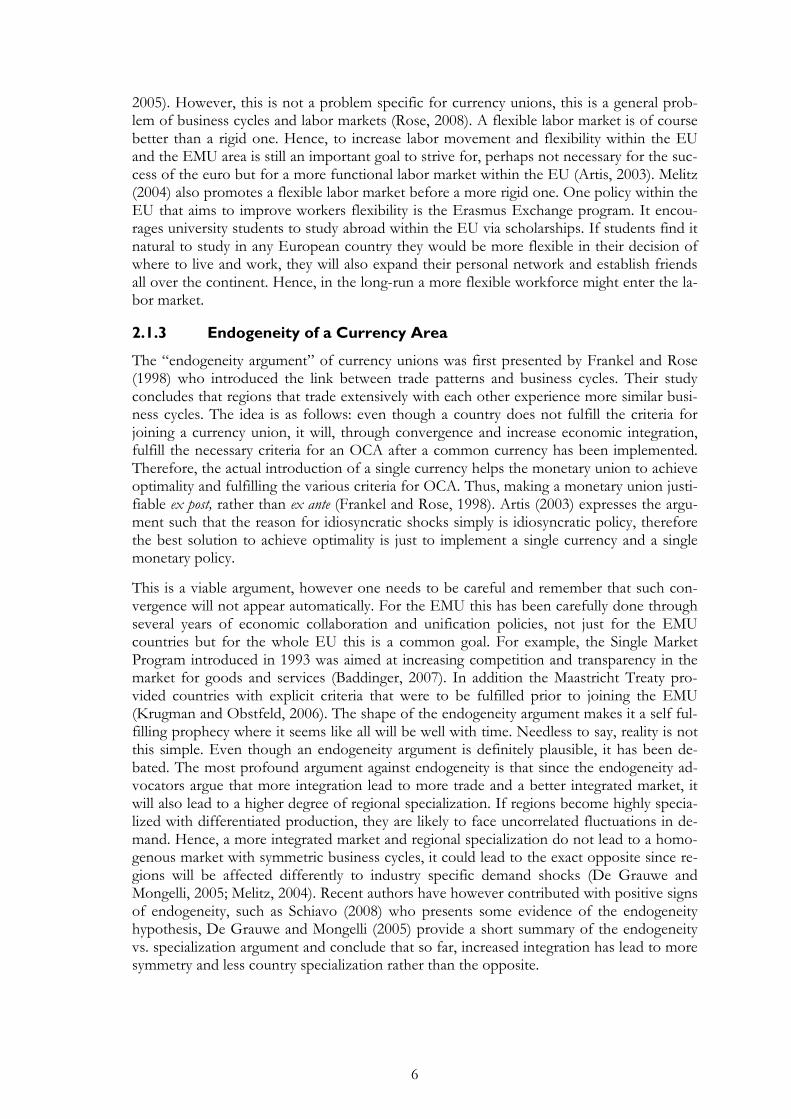
It is widely accepted that inflation and unemployment are related. The widely used frame-work is of course the Phillips Curve which traditionally is presented as a negative relation-ship between inflation and unemployment, although Phillips who introduced the relation-ship plotted wage inflation versus unemployment (Phillips, 1958; Dornbusch, 2008). The Phillips curve generally implies the relationship between unemployment and inflation, sug-gesting that it would be possible to increase inflation in order to boost employment. A li-near presentation of the relationship could look like this (Dornbusch, 2008)4:

� � �� �� (2.1)

Where � is the inflation rate, is the coefficient that provides a measurement for the res-

ponsiveness in inflation to changes in unemployment, � is the unemployment rate and ��is

the natural rate of unemployment. The bracket term �� �� denotes the change of un-employment in relation to the natural rate of unemployment. A simple linear interpretation of Equation (2.1) is illustrated in Figure 2-1. Noticeably, Equation (2.1) does not include an intercept term which normally we should expect when graphically presented as below. An intercept can of course be included, however, that would imply that we would observe an unemployment rate of zero percent that would correspond to a particular level of inflation. Generally, basic economic theory predicts that there will always be some unemployment present, at least some frictional unemployment (McDowell, 2006).

4 I present the Phillips Curve with general inflation and not wage inflation although this is the choice of

Dornbusch (2008)

8

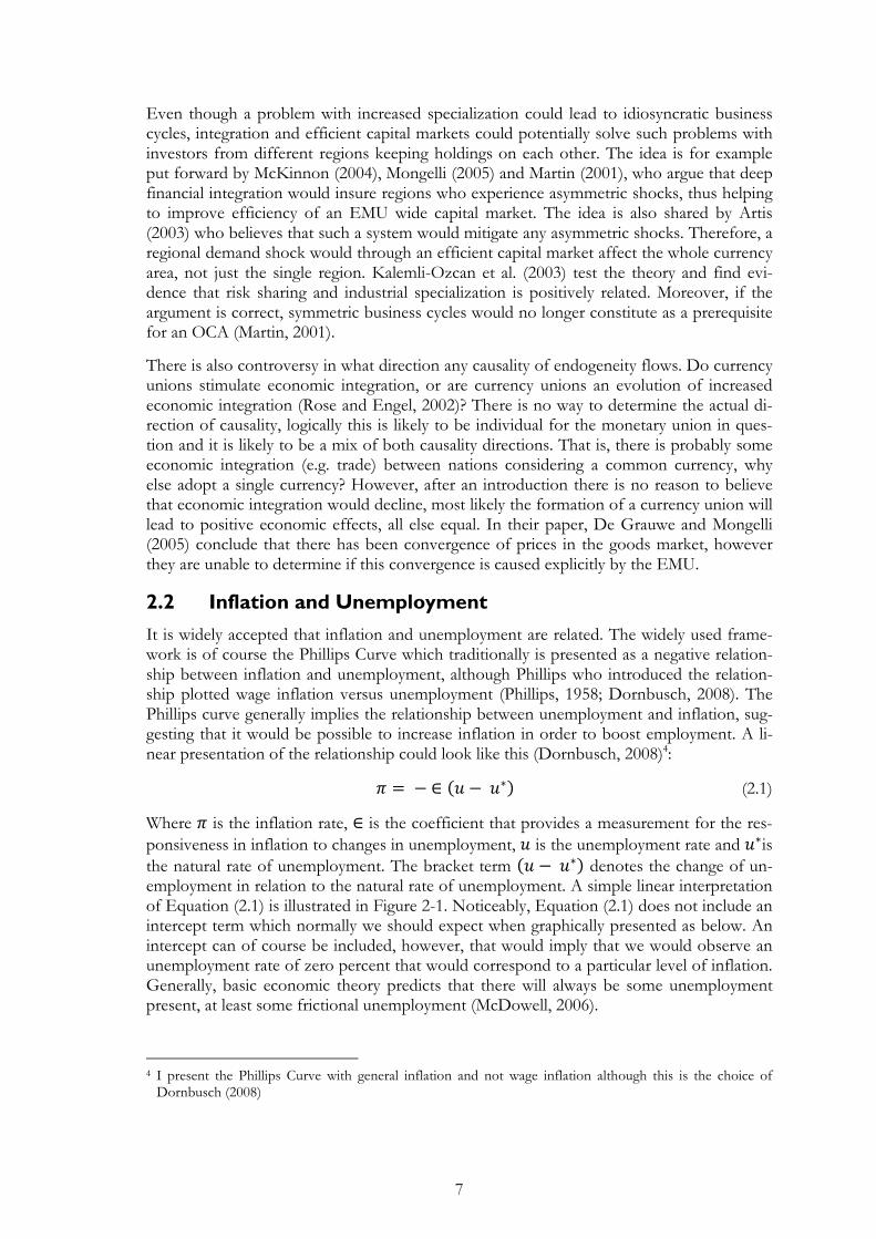
In the 1970’s and 1980’s the data no longer supported a simple Phillips Curve as it pre-viously did, there was something missing in the model. Therefore the new or augmented Phillips curve was introduced which included future expectation about inflation into the model. Following Equation (2.1),

� � �� �� �� (2.2)

Where the term �� in Equation (2.2) is included to account for future expectations of infla-tion. Therefore, changes in inflation will be related to changes in unemployment and future expectations of inflation. The simplest, and somewhat naive, way of thinking of how future expectations work is to take future expectations to equal actual inflation in the previous pe-

riod, that is �� � ����. Although expectations cannot be entirely based on past expe-riences, there will be some inertia in the structure of price and wage inflation. An example of this would be long-term wage contracts where wage increases are determined for a couple of years at a time (Dornbusch, 2008; Romer, 2006). Graphically, the change in ex-pectations would not affect the slope of the Phillips curve. Instead, an increase in the ex-pectations would shift the curve upward without a change in the slope parameter. This is il-lustrated below in Figure 2-2, where the curve is shifted upward into a higher position maintaining the same slope.

π

� Figure 2-1: Short-run Phillips Curve (Source: Dornbush (2008))

π

� Figure 2-2: Augmented Phillips Curve (source: Dornbush 2008)

9

Changes in unemployment can be used to measure cyclical positions and economic condi-tions. The relationship between unemployment and output is presented in Okun’s Law, which is formally stated as:

� �� � ��� �� (2.3)

Where � is actual output, �� is potential output. Thus making � �� the output gap,

which will be an expansionary gap when � is larger than ��, and a recessionary gap when �

is smaller than ��. � is the Okun coefficient which is traditionally estimated around three.

� is the unemployment rate and �� is natural or potential unemployment. �� and �� are

considered to be fixed in the short-run. �� �� is thus the difference in unemployment from natural unemployment (Prachowny, 1993). With the estimate of the Okun coefficient

it stems that a one percentage point decrease in the unemployment rate, �, requires the ac-

tual output, �, to increase by three times as much ((-3) * (-1) = 3), in order for the equality to hold given the change in the unemployment rate.

2.3 Monetary Policy

The primary objective of the ECB is to ensure price stability in the medium-run, which is defined as a yearly increase in the HICP (Harmonized Index of Consumer Prices) by 2 per-cent (ECB, 2005). This is achieved through an interest rate mechanism where the ECB’s main interest rate affects the financial markets and the market interest rates and thus sub-sequently it affects the spending and investment decisions by firms and private agents (ECB, 2000). A lower interest rate positively affects investment and spending since it low-ers the cost of credit. Therefore when the ECB, or any central bank, lowers its interest rate it will increase the aggregate demand in the economy, all else equal. In addition, a stimula-tion of aggregate demand would increase national income in the short-run (Dornbusch, 2008).

Differences in the economic institutions could possibly cause the interest rate and mone-tary policy from the ECB to affect national inflation rates differently. National characteris-tics, a more developed bank sector, differences in price and wage rigidity and future expec-tations of inflation might affect the national rates (Fendel and Frenkel, 2009). Therefore not only the one-size policy from the ECB but also symmetric shocks across the euro area could affect member nations differently (Hofmann and Remsperger, 2005).

These differences are not only caused by structural factors, but public preference for infla-tion influence how policies are shaped and remain important factors (Mongelli, 2005). The politics of inflation is complex and differ across the euro area, the likelihood that high in-flation is unpopular may cause national politicians to respond with extensive fiscal meas-ures. Possibly without knowing the real causes behind inflation causing ill advised policy actions (Honohan and Lane, 2005). In addition, individual nations may differ in their ability to conduct fiscal policy to combat inflation differences given their state of national finances (ECB, 2005). Thus, countries with weak national finances and larger debt or deficits will be compromised in their abilities to conduct fiscal policy in order to mitigate large swings in business cycles.

10

Debt structure, tax-credits and transfer payments may play a large role in determining the outcome of monetary policy. Haug et al. (2000) raise concerns that although the differences in budget deficits were reduced during the 1990’s, it may not cause absolute convergence in the long-run. They stress that the political structures are different in the euro countries and legislative differences concerning fiscal spending might constrain some countries while other countries are able to spend more and run larger deficits in a recession (Haug et al., 2000). Mongelli (2005), however, believe that the same convergence points to a political convergence that will be sustained through continuous work towards a common constitu-tional framework. It is mentioned that in line with the Maastricht Treaty, fiscal balances remains a necessary condition for the euro area members in order for the ECB to be able to conduct a successful “one-size-fits-all” monetary policy (ECB, 2005). In ECB (2005) it is stated that sound fiscal finances are crucial if regional adjustment is to function through na-tional fiscal policy, countries need to be able to rely on fiscal policy without running the risk of excessive deficits and thus creating large national debts. In addition, recent history suggests that some nations have not been effective in their use of fiscal instruments, in-stead there is evidence of pro-cyclical policies in recent past which have increased the cyc-lical differences (ECB, 2005).

11

3 Inflation in the EMU-12

3.1 Inflation Divergence

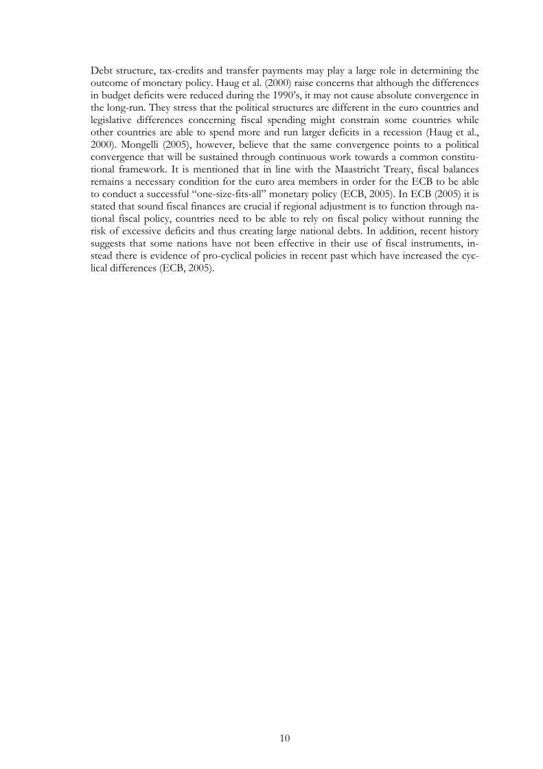
Recent literature have pointed out that prior to the euro introduction in 1999 the original EMU nations experienced convergence in several fiscal and monetary areas (ECB, 2003). Figure 3-1 plots annual HICP for the EMU-12.

Figure 3-1: Annual HICP for the EMU-12 countries, some observations before 1995 are missing (source: stats.oecd.org)

It is clear that the rates converges in the run up to 1999, it can also be noticed that after 1999 inflation rates increased and became more diverse. In addition, one can also clearly see that the average unweighted annual inflation was above 2 percent. In fact, even the official EMU average of HICP for all member countries was just above 2 percent for the years between 2000 and 2008, however only slightly above 2 percent.

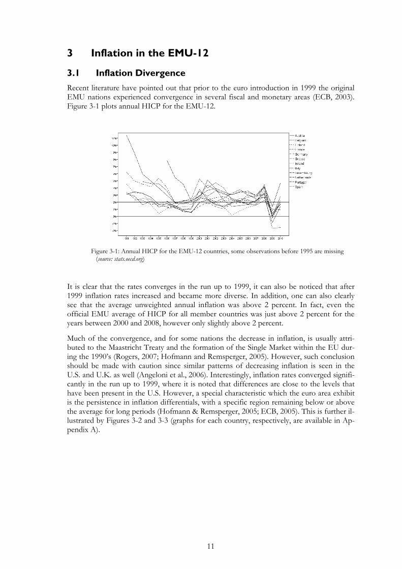
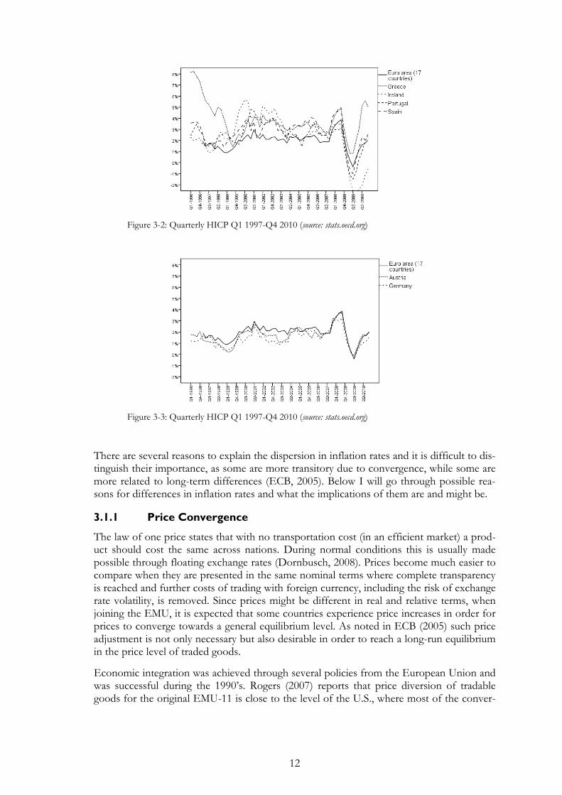
Much of the convergence, and for some nations the decrease in inflation, is usually attri-buted to the Maastricht Treaty and the formation of the Single Market within the EU dur-ing the 1990’s (Rogers, 2007; Hofmann and Remsperger, 2005). However, such conclusion should be made with caution since similar patterns of decreasing inflation is seen in the U.S. and U.K. as well (Angeloni et al., 2006). Interestingly, inflation rates converged signifi-cantly in the run up to 1999, where it is noted that differences are close to the levels that have been present in the U.S. However, a special characteristic which the euro area exhibit is the persistence in inflation differentials, with a specific region remaining below or above the average for long periods (Hofmann & Remsperger, 2005; ECB, 2005). This is further il-lustrated by Figures 3-2 and 3-3 (graphs for each country, respectively, are available in Ap-pendix A).

12

Figure 3-2: Quarterly HICP Q1 1997-Q4 2010 (source: stats.oecd.org)

Figure 3-3: Quarterly HICP Q1 1997-Q4 2010 (source: stats.oecd.org)

There are several reasons to explain the dispersion in inflation rates and it is difficult to dis-tinguish their importance, as some are more transitory due to convergence, while some are more related to long-term differences (ECB, 2005). Below I will go through possible rea-sons for differences in inflation rates and what the implications of them are and might be.

3.1.1 Price Convergence

The law of one price states that with no transportation cost (in an efficient market) a prod-uct should cost the same across nations. During normal conditions this is usually made possible through floating exchange rates (Dornbusch, 2008). Prices become much easier to compare when they are presented in the same nominal terms where complete transparency is reached and further costs of trading with foreign currency, including the risk of exchange rate volatility, is removed. Since prices might be different in real and relative terms, when joining the EMU, it is expected that some countries experience price increases in order for prices to converge towards a general equilibrium level. As noted in ECB (2005) such price adjustment is not only necessary but also desirable in order to reach a long-run equilibrium in the price level of traded goods.

Economic integration was achieved through several policies from the European Union and was successful during the 1990’s. Rogers (2007) reports that price diversion of tradable goods for the original EMU-11 is close to the level of the U.S., where most of the conver-

13

gence were obtained prior to the launch of the euro. So whether the euro, per se, has de-creased diversion or whether the achievement of deeper political ties and goals are the real reason, is less clear. Similar results are observed by Angeloni et al. (2006). Weber and Beck (2005) suggest that a convergence process might be non-linear, implying that convergence occurs quickly at first, but then decreases in speed the closer to unity countries come. This could offer an explanation why Rogers (2007) observe less convergence after 1999.

When the price level and productivity converge for tradable-goods, it means that there will be an upward pressure on wages in the goods sector which will cause the income levels to converge in the euro area. If labor is assumed mobile between sectors inside regions, it will create a tendency for wages and prices to rise in all sectors, raising price and wage in non-tradable sectors as well. This is what is referred to as the Balassa-Samuelsson (BS) effect, that although prices of tradable goods have converged, income of workers in the non-tradable sector could still cause a local price level to increase (Alberola and Tyrväinen 1998; Fendel and Frenkel, 2009).

The BS effect has been investigated by several authors, however recently its effect has be-come questioned and the reality of such an effect is not certain. Hofmann and Remsperger (2005) compare the results from seven studies between 1998 and 2002 and find a positive correlation between inflation and the BS effect. However, the same study finds that other factors were more important when explaining the causes for inflation differences. Altissimo et al. (2005) report that country specific productivity shocks in the non-traded goods sector can cause sizable inflation differentials in countries, suggesting that the BS effect might be present after all. Fendel and Frenkel (2009) reports that recent estimates of the BS effect are small, however the BS effect might become important when new members will join the EMU. To summarize, there is probably a tendency for a BS effect to exist, however, its im-portance is likely to differ between countries. More importantly, it is likely to be present only in the short-run (Fendel and Frankel, 2009; ECB, 2005). For the EMU-12, which is the focus of this study, transitory factors should not be present any longer.

3.1.2 Economic Transmission

Even when price convergence has reached its long-term equilibrium level, different charac-teristics on a country level may cause inflation to be affected differently. As mentioned in section 2.3, Haug et al. (2000) criticize the efforts to reduce the deficits in the 1990’s and point to the possibility that these might not be sustained permanently. Interestingly, given the recent events with the debt crisis that sparked from the financial downturn at the end of the decade, one must give credit to Haug et al. (2000) who actually hinted the reader of such possibilities more than a decade ago. It proves that monetary policy is much easier to change than fiscal policy, which has long term effects with a history that is harder to erase (Haug et al., 2000).

Table 3-1 provides a summary for how disperse the debt structure is for some of the EMU-12 states, it can be noted that Luxembourg is not included, but has since the forma-tion of the euro kept its national debt in single digits5. Noticeable increases are Greece, Portugal and Spain, where the debt is increasing rapidly with more than 10 percent points in 2009. However, the worst performance came from Ireland, whose debt increased by al-most 20 percentage points of GDP in 2009.

5 Austria and France are not included either, although they have kept their debt level and HICP in close rela-

tion with Germany.

14

Table 3-1: Central Government Debt % of GDP (source: stats.oecd.org)

Belgium Finland Germany Greece Ireland Italy Netherlands Portugal Spain

1998 105.3 59.9 26.1 103.7 47.8 108.7 52.0 54.8 53.6

1999 103.4 55.7 34.1 103.6 44.1 106.7 49.2 55.1 52.3

2000 99.5 48.0 34.1 108.9 34.8 103.6 44.1 54.1 49.9

2001 99.1 44.4 34.6 109.7 30.9 102.7 41.3 56.0 46.3

2002 97.9 41.3 36.1 109.2 27.9 99.5 41.5 58.7 43.9

2003 95.4 43.5 37.7 105.8 26.9 96.8 43.0 60.2 40.7

2004 92.8 41.9 39.2 108.3 25.4 96.2 43.8 63.0 39.3

2005 91.8 38.2 40.4 110.3 23.6 97.5 43.0 68.2 36.4

2006 87.6 35.6 40.9 107.5 20.3 96.7 39.2 69.8 33.0

2007 85.3 31.2 39.4 105.8 19.8 95.2 37.8 69.2 30.0

2008 90.2 29.5 38.8 109.6 27.7 98.0 50.1 71.2 33.7

2009 95.3 37.6 43.8 125.7 46.0 106.6 49.9 81.1 46.1

According to the Maastricht Treaty, nations were required to reduce their debt to 60 per-cent of GDP or to implement actions so that their debt levels would steadily decline to-wards 60 percent. In order to join the EMU, deficits are required to be no larger than 3 percent of GDP. After the start of the euro the Stability and Growth Pact (SGP) set out rules and procedures to act on if countries breached the SGP agreements (European Commission 2010). However, the SGP was reshaped in 2005 to allow more flexible rules and penalties when breached. As the table suggests, it is clear that all nations have not kept their financial stance within the agreed upon rules. In 2009, ten of the EMU-12 countries were in breach of the SGP and were placed by the council in the Excessive Deficit Proce-dure (EDP) and will be forced to correct the fiscal balances in the future (European Com-mission 2010)6.

Table 3-2 highlight the differences in annual inflation (HICP), where Ireland have expe-rienced deflation for two straight years while inflation in Greece, as mentioned, took off in 2010. The spread for 2010 is above 6 percentage points.

Table 3-2: Annual changes in HICP (source: stats.oecd.org)

Belgium Finland Germany Greece Ireland Italy Netherlands Portugal Spain

2002 1.55 2.01 1.35 3.92 4.72 2.61 3.87 3.68 3.59

2003 1.51 1.30 1.03 3.44 4.00 2.81 2.24 3.26 3.10

2004 1.86 0.14 1.79 3.03 2.30 2.27 1.38 2.51 3.05

2005 2.53 0.77 1.92 3.48 2.18 2.21 1.50 2.13 3.38

2006 2.34 1.27 1.78 3.31 2.70 2.22 1.65 3.04 3.56

2007 1.82 1.58 2.28 2.99 2.87 2.04 1.58 2.42 2.84

2008 4.49 3.91 2.75 4.23 3.11 3.50 2.21 2.65 4.13

2009 -0.01 1.64 0.23 1.35 -1.71 0.76 0.97 -0.90 -0.24

2010 2.33 1.69 1.15 4.70 -1.57 1.64 0.93 1.39 2.04

When these differences culminate the individual nations still have to operate in the same policy climate as all euro nations. However, the situation and circumstances in each country

6 All violations of the SGP are not highlighted in Table 3-1, for further information see European Commis-

sion (2010).

15

is different and thus highlight the possibility that nations may operate in separate cycles. In addition, the financial strength of an economy may affect the growth in output and hence affect the cyclical position of a country and through this channel affect national inflation (Hofmann and Remsperger, 2003). Although the current situation is very complex, one may question if both Greece and Ireland can benefit much from the same monetary policy at the moment.

It has also been mentioned that domestic preferences could affect countries differently through a “composition” effect. A general price shock in the whole euro area may affect demand differently since the domestic composition of HICP is not the same for all nations, this is natural since spending patterns are not the same. Therefore, inflation rates may be affected locally in the short-run. However, such differences have been calculated to have very small effects on inflation differentials, at most around 0.2 percent (Hofmann and Remsperger, 2005; Fendel and Frenkel, 2009).

3.1.3 Exchange Rate Volatility

Since the countries in the euro area depend differently on exports and imports to outside the euro area, a change in the exchange rate of the euro affects the countries differently (Fendel and Frenkel, 2009). The mechanism through where exchange rate movements af-fect national inflation is straight forward and works in two ways. A country (e.g. Ireland who trade a lot with the U.S. and the U.K.) whose economy depends, relatively to its euro members, more on exports to non-euro countries will be affected positively if the euro de-preciates, while other euro-nations might not be affected much of such a depreciation (Fendel and Frenkel, 2009). The increased exports stimulate the economy, exporting firms produce more profits, causing higher wages, pushing the price level to increase faster than in other euro nations (Dornbusch, 2008). In addition, prices of imported goods will in-crease and may shift the consumption to more domestically produced goods, increasing domestic demand further (Dornbusch, 2008). Such differences in non-euro trade patterns could potentially also cause problems with asymmetric shocks, where such a country would move into an expansion or recover faster through a euro-wide recession. In other words, such a country is likely to operate in a different business cycle (Honohan and Lane, 2003).

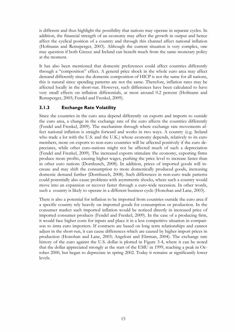
There is also a potential for inflation to be imported from countries outside the euro area if a specific country rely heavily on imported goods for consumption or production. In the consumer market such imported inflation would be noticed directly in increased price of imported consumer products (Fendel and Frenkel, 2009). In the case of a producing firm, it would face higher costs for inputs and place it in a less competitive situation in compari-son to intra euro importers. If contracts are based on long term relationships and cannot adjust in the short-run, it can cause differences which are caused by higher import prices in production (Honohan and Lane, 2003; Angeloni and Ehrman, 2004). The exchange rate history of the euro against the U.S. dollar is plotted in Figure 3-4, where it can be noted that the dollar appreciated strongly at the start of the EMU in 1999, reaching a peak in Oc-tober 2000, but began to depreciate in spring 2002. Today it remains at significantly lower levels.

16

Figure 3-4: USD-EUR Exchange Rate, measured as EUR per 1 USD, monthly averages (source: stats.oecd.org)

Honohan and Lane (2003) investigate the importance of exchange rate volatility and more precisely the implication of the depreciation of the euro against the U.S. dollar in early years of the euro. Their analysis concludes that the depreciation had a significant part of the inflation rate differences that were observed in the close years after the euro introduc-tion. Although, they lay a large weight on cyclical differences as well. This is in accordance with conclusion of Hofmann and Remsperger (2005) who argue that the observed differ-ences in inflation rates are mainly driven by exchange rate fluctuations and different cyclical patterns. However, the magnitude of the results are questioned by Angeloni and Ehrmann (2004) who credit exchange rate fluctuations as affecting the inflation rate, but credit persis-tence of inflation to be the most important reason for differences in inflation rates. Mone-tary transmission and asymmetric shocks are less important according to Angeloni and Ehrmann (2004).

3.2 Implications of Inflation Divergence

Given the causes listed above it is likely that we would observe inflation differentials to persist in the euro area for years to come (ECB, 2003), especially since new members are waiting to adapt the euro in the near future (Angeloni and Ehrmann, 2004). However, as this study focuses on the core countries that have been members since the start (Greece since 2001), and if there still is significant differences in their inflation rates, this is some-thing that needs to be investigated and possibly eliminated

The less uniformed inflation rates are within the euro area, the more difficult it will be for the ECB to conduct a monetary policy so that “one-size-fits-all”. In order to construct a monetary policy that keeps the euro area inflation below 2 percent will not be the ECB’s only concern. Instead, since the average is constructed through weighting the different economies in the area differently, larger weights are naturally given to larger and more “im-portant” economies7. An outlier nation could potentially affect the average to a large extent or, if the nation is small, have only modest effects on the average and therefore having to cope with a monetary policy that is not optimal (Aksoy et al., 2004). What worries is that a small country would become more frustrated than a large country if its inflation rate is not synchronized with the euro average, since the effect of its inflation rate would not affect

7 Current weights can be viewed at the ECB’s official website. However, Germany, France, Spain and Italy

carry above 75 percent of all weight. http://epp.eurostat.ec.europa.eu/portal/page/portal/hicp/data/database (Mars 16, 2011)

17

the average as much. It follows that a monetary policy under such circumstances will not be suited for the country in question (Aksoy et al., 2002; Hofmann and Remsperger, 2005). Thus the real difficulty lies in the ability to construct a monetary policy that is suitable for all countries using the euro, not just to keep a goal for average inflation. If the countries in-volved are not similar enough, the task becomes increasingly difficult. Noticeable, the ECB is in fact concerned about this problem, however, it remains a secondary objective (ECB, 2005).

The strategy implemented by the ECB currently is to keep euro area inflation below, but close to 2 percent per annum. There is no explicit goal to try to affect country specific in-flation, however it is stated that when constructing a policy, country differences are consi-dered and taken into account (ECB, 2005). The primary goal however, is to keep prices stable in the euro aggregate. Fendel and Frankel (2009) investigate if the ECB’s decisions are influenced by country specific differences, and conclude that the ECB do take differ-ences of inflation into consideration. Possibly the decision to keep inflation close to 2 per-cent is a policy aimed at reducing the risk of deflation in Germany (Fendel and Frankel, 2009).

It is natural for inflation to be diverse in the short-run, especially during a convergence pe-riod after the start of the union or for newly joined countries. Since new members are cur-rently adapting towards a membership, this is likely to remain a property within the EMU for years to come. Especially if new members from Central and East Europe exhibit large productivity asymmetries with the larger economies of Europe (Angeloni and Ehrmann, 2004). However, in the (very) long-run, price levels cannot move too far from unity, they would have to converge back towards an equilibrium level, at least for tradable goods. This is achieved given that real exchange rates only are concerned with relative prices and within a currency area these cannot move further and further apart (Hofmann and Remsperger, 2005).

In addition, if one credits the theory of endogeneity, those countries sharing a common currency would become more integrated and would eventually converge in price level the longer they share a currency. Then, one should not be concerned about differences in price movement in a long-run perspective. The support for this view is such that the countries within the euro area that are the most identical also experience the least price level fluctua-tions (Hofmann and Remsperger, 2005). Given the findings of Hofmann and Remsperger (2005), that cyclical position was the main factor contributing to inflation differences after the start of the euro, a more integrated economy would denote less persistent and less se-vere to country specific shocks from temporary demand or supply fluctuations, price level or exchange rate movements (see discussion above). A similar conclusion is made by ECB (2005) who, surprisingly, pose little concern over inflation differences. Although they rec-ognize their existence and persistence, they explain most of it as a desirable convergence, and little concern is given any other (negative) explanation.

Moreover, when non-members consider if they should join the EMU, an important aspect will be the possibility to achieve price stability with the help of a membership (i.e. the ac-cession to the euro would give any nation credibility for price stability). The euro can for some nations work as an anchoring currency, lowering inflation faster than possible on its own. This is an additional argument for why one would expect a convergence in the first years following the creation or joining of the euro area. Furthermore, it creates credibility for small economies as discussed above in section 2.1.1 (McKinnon, 2004; Mongelli, 2005). Although inflation is lowered for new members, it may still stay above average euro infla-tion. For the near future we might just have to live with the fact that inflation rates in the

18

euro area might act divergent in the short-run since more Central and East European coun-tries are getting set to join the EMU, some with a very high inflationary history (Angeloni and Ehrmann, 2004)8.

Up to this point the discussion has concerned causes and implications of higher than aver-age inflation. However, given that some are above average inflation, some nations naturally need to be below average, as was clearly illustrated by Figure 3-3 above. If the euro average would drop to levels below 1 percent there would be serious threats of a deflationary pres-sure in those countries that traditionally are low inflation countries, e.g. Germany and France (Weber and Beck 2005). Even though this is not a probable scenario in the long-run, deflation is worrying already in the short-run. Moreover, a 1 percent deflation is more severe and less accepted publically than a 1 percent above average inflation. Therefore sug-gestions have been made to state an explicit lower target for inflation (Weber and Beck, 2005; von Hagen and Hofmann, 2004). However, empirical evidence from the actual poli-cies of the ECB suggest that the HICP is kept close to 2 percent (Fendel and Frenkel, 2009), which indeed the ECB state they intend to do (ECB, 2005). Furthermore, Fendel and Frenkel (2009) raise concerns that although the ECB would like to aim policies to combat inflation in countries where it is above average it might be reluctant to do so since there are nations on the other side of the scale that potentially would experience deflation. They conclude that the ECB do take inflation differentials into consideration when they decide upon monetary policy (Fendel and Frenkel, 2009), potentially to prevent a deflatio-nary pressure in for example Germany. This is also what is mentioned in ECB (2003 and 2005), however the primary goal remains to be price stability in the euro area as a whole.

8 Examples include Romania, Poland, Bulgaria, Hungary and Lithuania. A good graphical presentation of EU

member states inflation history since the mid 1990’s can be viewed at the ECB’s homepage. http://www.ecb.int/stats/prices/hicp/html/inflation.en.html (May 20, 2011).

19

4 Empirical Investigation

To analyse the movement of inflation rates in the euro area, a Phillips Curve like model is constructed to investigate how changes in unemployment compared to the EMU average affect the national inflation rate. The purpose is not to pinpoint any divergent pattern in in-flation movements, but to investigate if the “Phillips coefficient” is significantly different across countries of the EMU-12, causing national unemployment changes to affect infla-tion rates differently across the EMU-12. The model is constructed using a balanced panel data set where country specific fixed effects are included to incorporate any national differ-ences outside the model. The sample contains data for the EMU-12 nations and 50 obser-vations for each nation respectively. Since the model includes a lagged variable, the first observation is lost, thus making the total number of observations tested equal to 588.

As mentioned, this thesis makes use of panel data. The advantage with panel estimation is that it uses both cross sectional and time series data. Here, the cross sectional term is the countries of the EMU-12 and the time series is simply all quarters ranging from the second quarter in 1998 to the third quarter in 2010. A specific advantage of using panel data in this analysis, is that we are able to account for any underlining country specific heterogeneity that could otherwise compromise the result. If believed that these country specific effects were to vary over time we could include a fixed effect for time periods as well. A model like this which includes fixed effects is often referred to a fixed effects model (FEM) (Gu-jarati, 2009).

Instead of using fixed effects in a panel data estimation, one can use random effects. Guja-rati (2009) gives the suggestion that a random effects model (REM) can be suitable for when the data used for testing is drawn from a much larger population. However, this study focuses on 12 nations within the EMU, hence they do not make up a random sample of a larger population. The 12 nations make up the population themselves. To determine if a REM or FEM is appropriate, one can apply the Hausman test which is conveniently available in EViews. When performed, the null hypothesis is that the FEM and REM esti-mators do not differ significantly. If rejected, the FEM is believed to be more appropriate (Gujarati, 2009). The results from the Hausman test are available in Appendix C.

4.1 Model

The general model is constructed to test if the national Phillips coefficient is any different from the EMU average. The model is derived directly from the augmented Phillips curve presented in chapter 2. Basically the interpretation is that there are two Phillips curves merged into one estimations, which then are compared via a ratio in order to determine if they are different from each other. Therefore, I will be able to compare if the EMU-12 and the EMU average have the same Phillips coefficient or not. If the Phillips coefficient is dif-

ferent, � will be different from one (1) and would suggest that the EMU-12 is not equally sensitive to changes in unemployment as the EMU average. The model is developed from the merged Phillips curve which is specified in Equation (4.1).

��,�����,�

� ������

� ��,�� ���

����,� � ����� � � � ��,�������,���

� (4.1)

20

The econometric model which is then used for testing is presented below in Equation (4.2) and a simplified version is given in Equation (4.3).

��,�����,�

� ������

� ��,�����,� � � ! � ��,���

����,���� � "� � #�,� (4.2)

���,� � �$���,�% � !$���,���% � "� � #�,� (4.3)

Where � is the inflation rate, is the intercept, � is the Phillips coefficient which is as-

sumed to be negative. � is the unemployment rate, "� is the country specific fixed effect

and the subscripts j, t, and emu note the country, time period and the EMU average respec-

tively. ��is denoting the natural rate of unemployment. In order to include a control varia-

ble for future expectations for inflation the dependent variable is lagged one period, ! is

the coefficient which measure the effect of future expections. For Equation (4.3), ���,� is a

simplification of the dependent variable in Equation (4.2), the ratio between each nation

and the EMU average, and simply a relabeling. ���,� is a relabeling of the first parenthesis in

Equation (4.2). The natural rate of unemployment, which is not observed, is left to be ab-

sorbed by the country specific fixed effect, "� . Thus ���,�, is the ratio between national un-

employment rates and the EMU average unemployment rate. Algebraically this would look like:

��,�����,�

� ���,� (4.4)

��,�����,� � ���,� (4.5)

The ratios of inflation and unemployment were calculated before the regressions were made. Therefore, the actual model estimated is Equation (4.3), although the original prob-lem was specified as Equation (4.2). In addition, the model is also estimated with fixed ef-fects for time periods only, and one estimation with both time periods and country specific fixed effects. Those equations are presented below. Equation (4.6) includes fixed effects for

different time periods and is represented by &� . In Equation (4.7) both "� and &� included,

thus the equation includes both types of fixed effects.

���,� � �$���,�% � !$���,���% � &� � #�,� (4.6)

���,� � �$���,�% � !$���,���% � "� � &� � #�,� (4.7)

21

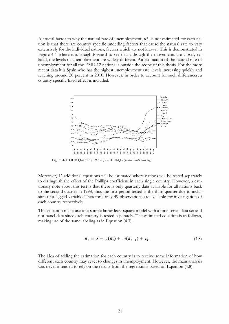
A crucial factor to why the natural rate of unemployment, �*, is not estimated for each na-tion is that there are country specific underling factors that cause the natural rate to vary extensively for the individual nations, factors which are not known. This is demonstrated in Figure 4-1 where it is straightforward to see that although the movements are closely re-lated, the levels of unemployment are widely different. An estimation of the natural rate of unemployment for all the EMU-12 nations is outside the scope of this thesis. For the more recent data it is Spain who has the highest unemployment rate, levels increasing quickly and reaching around 20 percent in 2010. However, in order to account for such differences, a country specific fixed effect is included.

Figure 4-1: HUR Quarterly 1998-Q2 - 2010-Q3 (source: stats.oecd.org)

Moreover, 12 additional equations will be estimated where nations will be tested separately to distinguish the effect of the Phillips coefficient in each single country. However, a cau-tionary note about this test is that there is only quarterly data available for all nations back to the second quarter in 1998, thus the first period tested is the third quarter due to inclu-sion of a lagged variable. Therefore, only 49 observations are available for investigation of each country respectively.

This equation make use of a simple linear least square model with a time series data set and not panel data since each country is tested separately. The estimated equation is as follows, making use of the same labeling as in Equation (4.3):

��� � '���� � !������ � #� (4.8)

The idea of adding the estimation for each country is to receive some information of how different each country may react to changes in unemployment. However, the main analysis was never intended to rely on the results from the regressions based on Equation (4.8).

22

4.2 Data

All data in this thesis is retrieved from the OECD database (stats.oecd.org) for statistics. For the empirical investigation the data used are quarterly observations of HICP (Harmo-nized Index of Consumer Prices) and HUR (Harmonized Unemployment Rate), both of which are developed by Eurostat for comparison of the nations within the EU. The OECD database was chosen due to its simplicity and better practicality, as compared to Eurostat. However, Eurostat was used as comparison of the data, and more importantly there were no differences in the two data sources.

In order to construct a balanced panel data set, HICP and HUR was used from the second quarter in 1998 up to the third quarter of 2010. Data was not available for all countries be-fore or after these dates. It is important to note that the EMU average is constructed and given by the OECD database. Since the composition of countries that are part of the EMU is different during the analyzed period the EMU average will include different coun-tries and different weights for particular countries. The EMU average is the actual EMU average, it is not an average of the EMU-12.

4.3 Descriptive Statistics

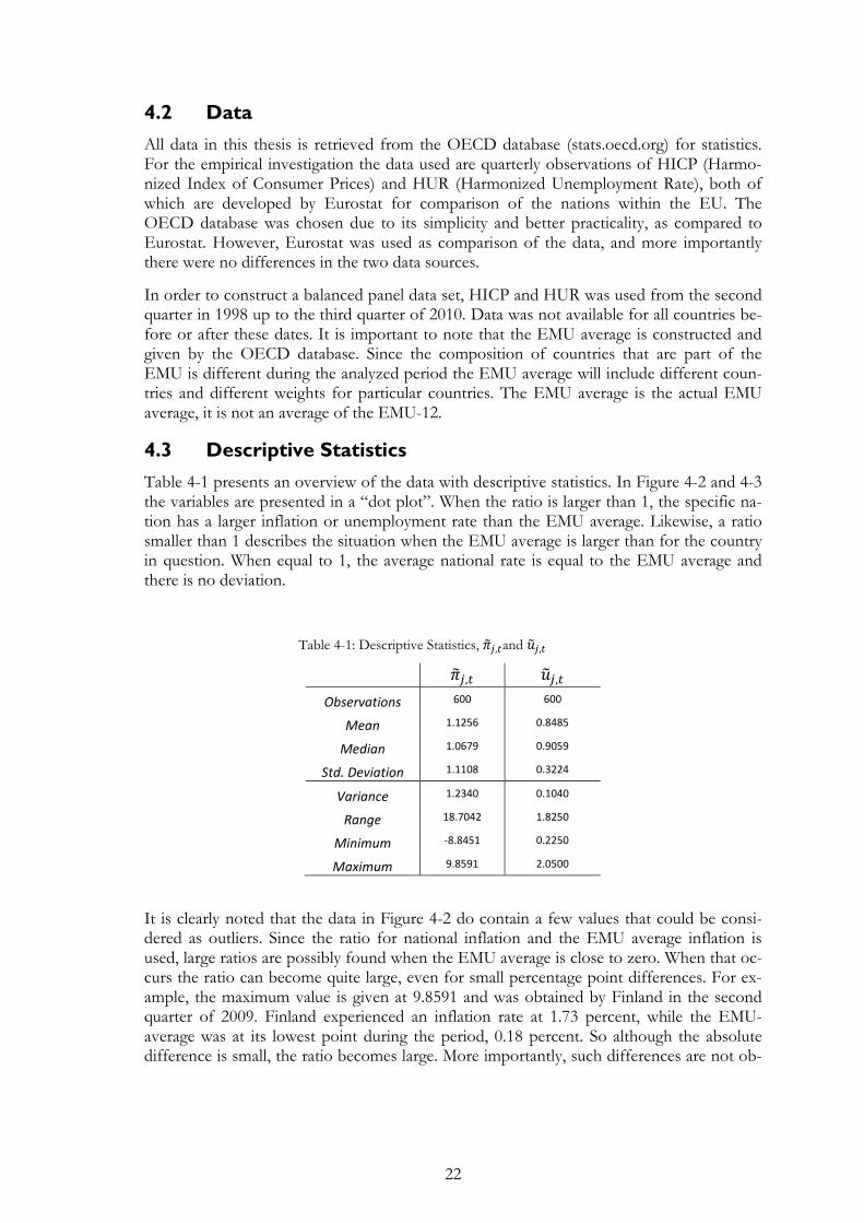
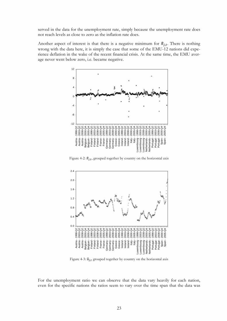
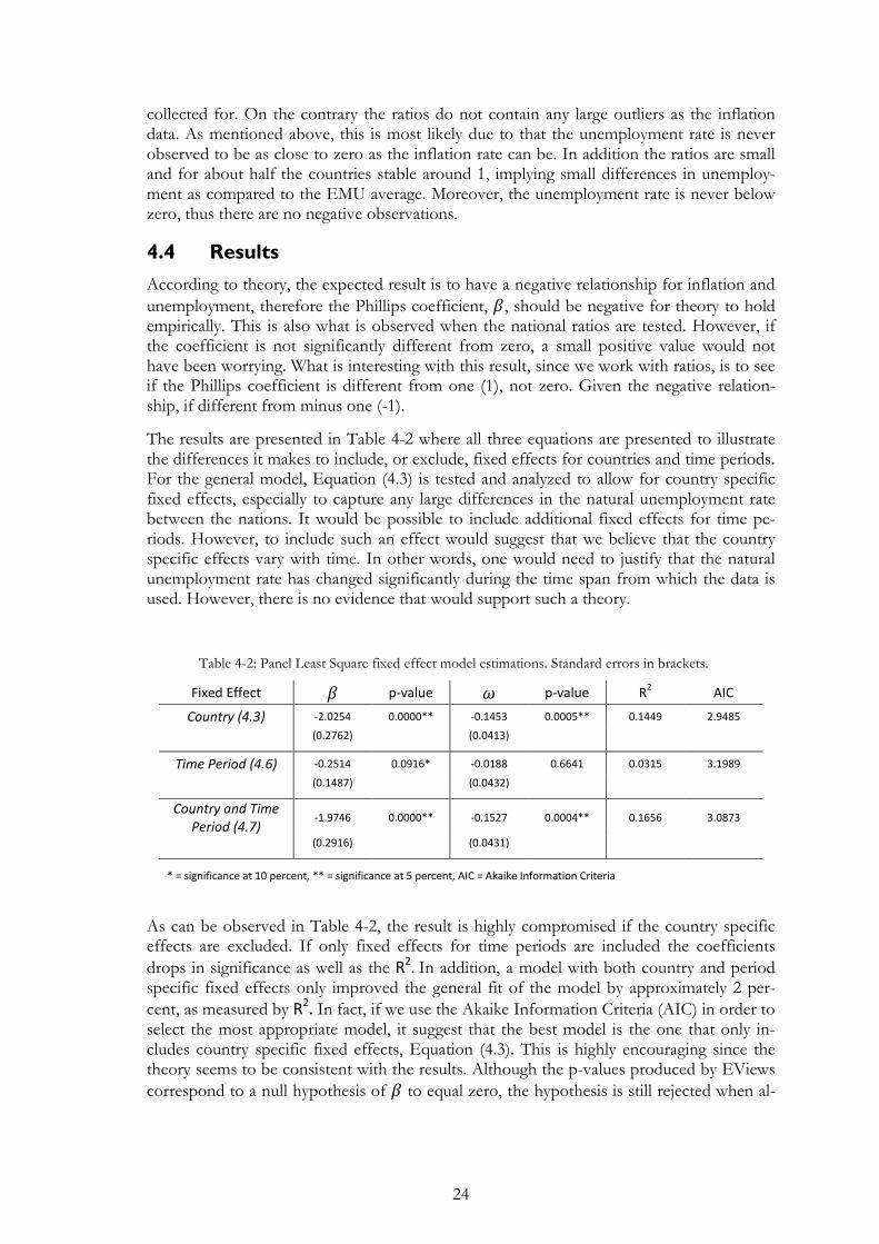
Table 4-1 presents an overview of the data with descriptive statistics. In Figure 4-2 and 4-3 the variables are presented in a “dot plot”. When the ratio is larger than 1, the specific na-tion has a larger inflation or unemployment rate than the EMU average. Likewise, a ratio smaller than 1 describes the situation when the EMU average is larger than for the country in question. When equal to 1, the average national rate is equal to the EMU average and there is no deviation.

Table 4-1: Descriptive Statistics, ���,�and ���,�

���,� ���,�

Observations 600 600

Mean 1.1256 0.8485

Median 1.0679 0.9059

Std. Deviation 1.1108 0.3224

Variance 1.2340 0.1040

Range 18.7042 1.8250

Minimum -8.8451 0.2250

Maximum 9.8591 2.0500

It is clearly noted that the data in Figure 4-2 do contain a few values that could be consi-dered as outliers. Since the ratio for national inflation and the EMU average inflation is used, large ratios are possibly found when the EMU average is close to zero. When that oc-curs the ratio can become quite large, even for small percentage point differences. For ex-ample, the maximum value is given at 9.8591 and was obtained by Finland in the second quarter of 2009. Finland experienced an inflation rate at 1.73 percent, while the EMU-average was at its lowest point during the period, 0.18 percent. So although the absolute difference is small, the ratio becomes large. More importantly, such differences are not ob-

23

served in the data for the unemployment rate, simply because the unemployment rate does not reach levels as close to zero as the inflation rate does.

Another aspect of interest is that there is a negative minimum for ���,�. There is nothing

wrong with the data here, it is simply the case that some of the EMU-12 nations did expe-rience deflation in the wake of the recent financial crisis. At the same time, the EMU aver-age never went below zero, i.e. became negative.

Figure 4-2: ���,� , grouped together by country on the horizontal axis

Figure 4-3: ���,� grouped together by country on the horizontal axis

For the unemployment ratio we can observe that the data vary heavily for each nation, even for the specific nations the ratios seem to vary over the time span that the data was

-12

-8

-4

0

4

8

12

Aus

tria

- 1

998-

Q2

Aus

tria

- 2

003-

Q2

Aus

tria

- 2

008-

Q2

Bel

gium

- 2

000-

Q4

Bel

gium

- 2

005-

Q4

Fin

land

- 1

998-

Q2

Fin

land

- 2

003-

Q2

Fin

land

- 2

008-

Q2

Fra

nce

- 20

00-Q

4F

ranc

e -

2005

-Q4

Ger

man

y -

1998

-Q2

Ger

man

y -

2003

-Q2

Ger

man

y -

2008

-Q2

Gre

ece

- 20

00-Q

4G

reec

e -

2005

-Q4

Irel

and

- 19

98-Q

2Ir

elan

d -

2003

-Q2

Irel

and

- 20

08-Q

2It

aly

- 20

00-Q

4It

aly

- 20

05-Q

4Lu

xem

bour

g -

1998

-Q2

Luxe

mbo

urg

- 20

03-Q

2Lu

xem

bour

g -

2008

-Q2

Net

herla

nds

- 20

00-Q

4N

ethe

rland

s -

2005

-Q4

Por

tuga

l - 1

998-

Q2

Por

tuga

l - 2

003-

Q2

Por

tuga

l - 2

008-

Q2

Spa

in -

200

0-Q

4S

pain

- 2

005-

Q4

0.0

0.4

0.8

1.2

1.6

2.0

2.4

Aus

tria

- 1

998-

Q2

Aus

tria

- 2

003-

Q2

Aus

tria

- 2

008-

Q2

Bel

gium

- 2

000-

Q4

Bel

gium

- 2

005-

Q4

Fin

land

- 1

998-

Q2

Fin

land

- 2

003-

Q2

Fin

land

- 2

008-

Q2

Fra

nce

- 20

00-Q

4F

ranc

e -

2005

-Q4

Ger

man

y -

1998

-Q2

Ger

man

y -

2003

-Q2

Ger

man

y -

2008

-Q2

Gre

ece

- 20

00-Q

4G

reec

e -

2005

-Q4

Irel

and

- 19

98-Q

2Ir

elan

d -

2003

-Q2

Irel

and

- 20

08-Q

2It

aly

- 20

00-Q

4It

aly

- 20

05-Q

4Lu

xem

bour

g -

1998

-Q2

Luxe

mbo

urg

- 20

03-Q

2Lu

xem

bour

g -

2008

-Q2

Net

herla

nds

- 20

00-Q

4N

ethe

rland

s -

2005

-Q4

Por

tuga

l - 1

998-

Q2

Por

tuga

l - 2

003-

Q2

Por

tuga

l - 2

008-

Q2

Spa

in -

200

0-Q

4S

pain

- 2

005-

Q4

24

collected for. On the contrary the ratios do not contain any large outliers as the inflation data. As mentioned above, this is most likely due to that the unemployment rate is never observed to be as close to zero as the inflation rate can be. In addition the ratios are small and for about half the countries stable around 1, implying small differences in unemploy-ment as compared to the EMU average. Moreover, the unemployment rate is never below zero, thus there are no negative observations.

4.4 Results

According to theory, the expected result is to have a negative relationship for inflation and

unemployment, therefore the Phillips coefficient, �, should be negative for theory to hold empirically. This is also what is observed when the national ratios are tested. However, if the coefficient is not significantly different from zero, a small positive value would not have been worrying. What is interesting with this result, since we work with ratios, is to see if the Phillips coefficient is different from one (1), not zero. Given the negative relation-ship, if different from minus one (-1).

The results are presented in Table 4-2 where all three equations are presented to illustrate the differences it makes to include, or exclude, fixed effects for countries and time periods. For the general model, Equation (4.3) is tested and analyzed to allow for country specific fixed effects, especially to capture any large differences in the natural unemployment rate between the nations. It would be possible to include additional fixed effects for time pe-riods. However, to include such an effect would suggest that we believe that the country specific effects vary with time. In other words, one would need to justify that the natural unemployment rate has changed significantly during the time span from which the data is used. However, there is no evidence that would support such a theory.

Table 4-2: Panel Least Square fixed effect model estimations. Standard errors in brackets.

Fixed Effect � p-value ! p-value R2

AIC

Country (4.3) -2.0254 0.0000** -0.1453 0.0005** 0.1449 2.9485

(0.2762) (0.0413)

Time Period (4.6) -0.2514 0.0916* -0.0188 0.6641 0.0315 3.1989

(0.1487) (0.0432)

Country and Time

Period (4.7) -1.9746 0.0000** -0.1527 0.0004** 0.1656 3.0873

(0.2916) (0.0431)

* = significance at 10 percent, ** = significance at 5 percent, AIC = Akaike Information Criteria

As can be observed in Table 4-2, the result is highly compromised if the country specific effects are excluded. If only fixed effects for time periods are included the coefficients

drops in significance as well as the R2. In addition, a model with both country and period specific fixed effects only improved the general fit of the model by approximately 2 per-

cent, as measured by R2. In fact, if we use the Akaike Information Criteria (AIC) in order to

select the most appropriate model, it suggest that the best model is the one that only in-cludes country specific fixed effects, Equation (4.3). This is highly encouraging since the theory seems to be consistent with the results. Although the p-values produced by EViews

correspond to a null hypothesis of � to equal zero, the hypothesis is still rejected when al-

25

tered to test for a null hypothesis equal to minus one (-1). Therefore, the Phillips coeffi-cient for the EMU-12 nations is not equal to the Phillips coefficient of the EMU average. In fact, the EMU-12 is more sensitive to unemployment changes than the EMU average.

The actual meaning of the results is interpreted as follows: when the unemployment rate

ratio (���,�) increases by one unit, the inflation rate ratio (���,�) is expected to fall by 2.0254

units, on average, as illustrated by �. The estimated value of the coefficient is of less impor-tance, the sign and that it is significantly different from one is of more importance. The

meaning of this is that when the value of the unemployment rate ratio (���,�) increases, the

lower is the value of the inflation rate ratio (���,�). Depending on the value of (���,�), the dis-

tance to the EMU average increases or decreases. If below 1, an increasing (���,�) term

pushes the nation in question further below the EMU average.

To make the interpretation more clearly, keep in mind what the ratios were made up of:

��,�����,� � ���,�

��,�����,�

� ���,�

So a decrease of the inflation ratio (���,�) could mean either a movement towards the EMU

average, or a movement away from the average. In other words, if the ratio becomes closer to 1 or not depends on the previous value of the variable. It only implies an increase (or decrease) of the actual value of the variable. Algebraically it would look like this:

���,� ( � ���,� )

The expectation coefficient, !, measures how the past inflation ratio affect the current in-

flation ratio. If the past inflation ratio (�����) increases by one unit, the inflation ratio at the

current period (���) decrease by an estimated 0.1453 units. In other words, a large differ-ence in the inflation rate at the current period, is expected to become smaller in the next period, however the convergence is expected to be very small. As noted earlier in the text, this corresponds to earlier evidence that inflation differences in the euro area are very per-sistent. On the other hand, some convergence is natural since inflation (or prices) cannot keep move further and further apart within a currency area, as mentioned above in section 3.2 (Hofmann and Remsperger, 2005). However, past inflation is included as a control va-riable to account for future expected inflation and is not the focus of the analysis.

In order to continue the analysis, a natural step is to test the countries separately as com-pared to the EMU average. Table 4-3 presents the result for the country specific model as estimated by Equation (4.8). The result is widely different at the national level.

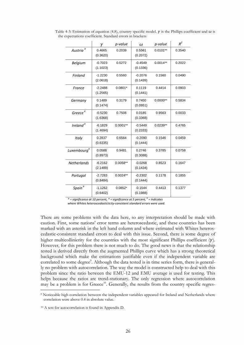
26

Table 4-3: Estimation of equation (4.8), country specific model. ' is the Phillips coefficient and ! is the expectations coefficient. Standard errors in brackets

' p-value ! p-value R2

Austria ¤ 0.4665 0.2039 0.5561 0.0101** 0.3540

(0.3620) (0.2072)

Belgium -0.7023 0.5272 -0.4549 0.0014** 0.2022

(1.1023) (0.1336)

Finland -1.2230 0.5560 -0.2076 0.1560 0.0490

(2.0618) (0.1439)

France -2.2488 0.0801* 0.1119 0.4414 0.0903

(1.2565) (0.1441)

Germany 0.1489 0.3179 0.7450 0.0000** 0.5834

(0.1474) (0.0951)

Greece ¤ -0.5230 0.7508 0.0185 0.9563 0.0033

(1.6368) (0.3368)

Ireland ¤ -6.1829 0.0001** -0.5449 0.0239** 0.4765

(1.4694) (0.2333)

Italy 0.2837 0.6564 -0.2090 0.1546 0.0459

(0.6335) (0.1444)

Luxembourg¤ 0.0588 0.9481 0.2746 0.3785 0.0758

(0.8973) (0.3088)

Netherlands -6.2162 0.0058** -0.0268 0.8523 0.1647

(2.1489) (0.1434)

Portugal -2.7283 0.0024** -0.2302 0.1178 0.1855

(0.8484) (0.1444)

Spain ¤ -1.1262 0.0852* -0.1544 0.4413 0.1377

(0.6402) (0.1988)

* = significance at 10 percent, * = significance at 5 percent, ¤ = indicates

where Whites heteroscedasticticity-consistent standard errors were used.

There are some problems with the data here, so any interpretation should be made with caution. First, some nations’ error terms are heteroscedastic, and these countries has been marked with an asterisk in the left hand column and where estimated with Whites heteros-cedastic-consistent standard errors to deal with this issue. Second, there is some degree of

higher multicollinierity for the countries with the most significant Phillips coefficient ('). However, for this problem there is not much to do. The good news is that the relationship tested is derived directly from the augmented Phillips curve which has a strong theoretical background which make the estimations justifiable even if the independent variable are correlated to some degree9. Although the data tested is in time series form, there is general-ly no problem with autocorrelation. The way the model is constructed help to deal with this problem since the ratio between the EMU-12 and EMU average is used for testing. This helps because the ratios are trend-stationary. The only regression where autocorrelation may be a problem is for Greece10. Generally, the results from the country specific regres- 9 Noticeable high correlation between the independent variables appeared for Ireland and Netherlands where

correlation were above 0.4 in absolute value.

10 A test for autocorrelation is found in Appendix D.

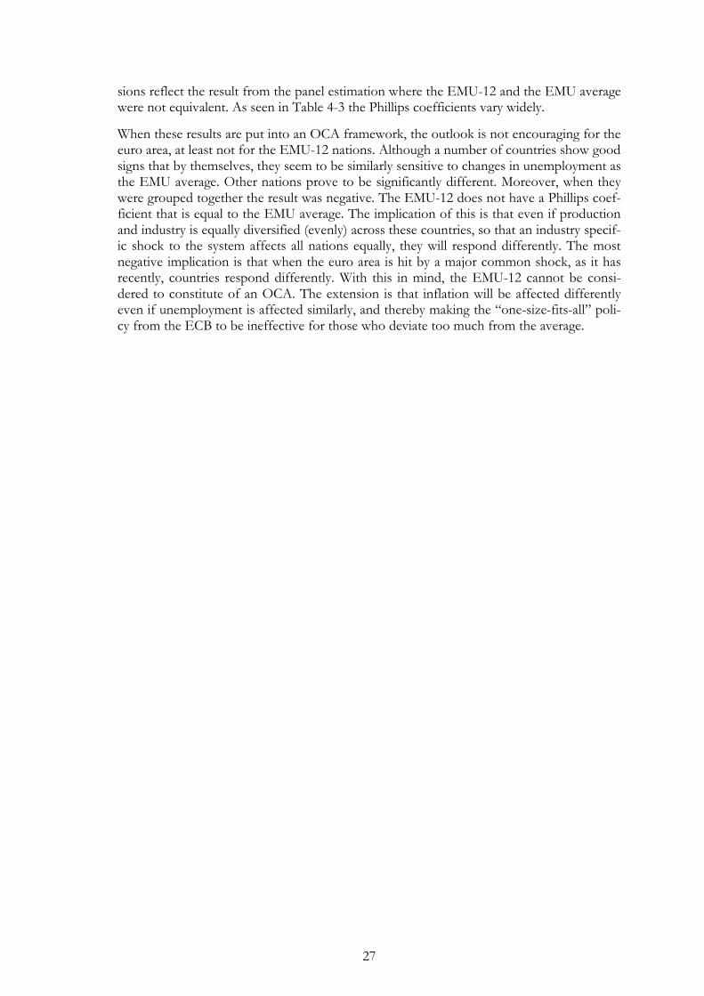
27

sions reflect the result from the panel estimation where the EMU-12 and the EMU average were not equivalent. As seen in Table 4-3 the Phillips coefficients vary widely.

When these results are put into an OCA framework, the outlook is not encouraging for the euro area, at least not for the EMU-12 nations. Although a number of countries show good signs that by themselves, they seem to be similarly sensitive to changes in unemployment as the EMU average. Other nations prove to be significantly different. Moreover, when they were grouped together the result was negative. The EMU-12 does not have a Phillips coef-ficient that is equal to the EMU average. The implication of this is that even if production and industry is equally diversified (evenly) across these countries, so that an industry specif-ic shock to the system affects all nations equally, they will respond differently. The most negative implication is that when the euro area is hit by a major common shock, as it has recently, countries respond differently. With this in mind, the EMU-12 cannot be consi-dered to constitute of an OCA. The extension is that inflation will be affected differently even if unemployment is affected similarly, and thereby making the “one-size-fits-all” poli-cy from the ECB to be ineffective for those who deviate too much from the average.

28

5 Summary and Conclusions

This thesis has investigated the cause, and what implication, divergent inflation rates may have for the success of the euro in an OCA context. The thesis has focused solely on the economic aspects of the euro and the EMU. There has been no effort to try to find other positive effects or benefits of currency unions such as political or psychological factors. In addition, it has also contributed with an empirical investigation which compares the Phillips coefficient of the EMU-12 countries to the EMU average. Moreover, comparisons were al-so made at country specific level.

It is my belief that the results has been shaped by the events in the world economy in re-cent years, however, it is times like these that put monetary unions to test. There are never any problems when all economies are experiencing a steady growth and all is well. The conclusion is that the EMU-12 nations that have been using the euro since 1999 (Greece since 2001), are not integrated enough to be able to react and fight a large common shock to the system collectively, as we have been experiencing in recent years. Countries are clear-ly affected, and are able to respond, very differently. This makes the conclusion negative for the success of the euro at present. The EMU is not an Optimum Currency Area.

The results are extremely up-to-date and point to the problems that are currently present within the euro area which have become apparent due to recent events. Since unemploy-ment became more diverse in the last couple of years, the model predicts that inflation have become more diverse as well. This causes the monetary policy governed the ECB to be unsuitable for some nations. Part of the problem is due to the different strengths of in-dividual countries’ national finances, which have required some nations to cut government spending significantly, which prolongs the effect of a recession.

The success of a single monetary policy has definitely been put to the test during the cur-rent crisis. When I write this, it was about one month ago (April 13th) that the ECB raised its interest rate with 0.25 percent (ecb.int, 2011). One week prior to the raise, Portugal was forced to ask the EU for financial support due to its increased debt and deficit. Obviously, an increase in interest rate resulted in a tightening of the monetary supply and did not help the Portuguese government to make the situation better. In fact, the decision to raise the main interest rate was taken on April 7 by the ECB, while Portugal declared its need for fi-nancial help only one day earlier, on the April 6 (di.se, 2011; bbc.co.uk, 2011).

Any reasons for why the nations respond differently is left for further research to be inves-tigated. One possible reason may be that different nations have different possibilities to conduct any successful fiscal policy in times of recessions or that unemployment benefits and labor market regulations cause unemployment to affect inflation differently. However, these suggestions are only speculative. For a clear picture, more research must be con-ducted.

List of references

29

List of references

Alberola, E. and Tyrväinen, T. (1998) ‘Is There Scope for Inflation Differentials in EMU? An Empirical Evaluation of the Balassa-Samuelson Model in EMU Countries’, Bank of Finland Dis-cussion Papers, 15/1998.

Altissimo, C., Benigno, P. and Palenzuela D.R. (2005) ‘Long-run determinants of inflation diffe-rentials in a monetary union’, CEPR Discussion Paper No. 5149, London.

Aksoy, Y., De Grauwe, P. and Dewachter, H. (2001) ‘Do asymmetries matter for Euroepan monetary policy?’ European Economic Review, Vol. 46, No. 3, pp. 443-469.

Angeloni, I., Aucremanne, L. and Ciccarelli, M. (2006) ‘Price setting and inflation persis-tence: did EMU matter?’ Economic Policy, Vol. 21, No. 46, pp. 353-387.

Angeloni, I. and Ehrmann, M. (2004) ‘Euro Area Inflation Differentials’ , Working paper se-ries, European Central Bank, No. 388, September 2004.

Arestis, P., Brown, A. and Malcolm, S. (2001), ‘The euro: evolution and prospect’, Edgar Elgar Publishing Limited, UK, Cheltenham.

Artis, M.J. (2003) ‘Reflections on the Optimal Currency Area (OCA) Critera in the Light of EMU’ International Journal of Finance and Economics, Vol. 8, No. 4, pp. 297-307.

Badinger, H. (2007) ‘Has the EU’s Single Market Programme Fostered Competition? Test-ing for a Decrease in Mark-up Rations in EU Industries’ Oxford Bulletin of Economics and Sta-tistics, Vol. 69, No. 4, pp. 497-519.

Baldwin, R, (2006), ‘In or Out: An Evidence based analysis of the euro’s effects’, Centre for com-parative European policy evaluation, London, U.K

Bayoumi, T. and Eichengreen, B. (1997) ‘Ever closer to heaven? An optimum-currency-area index for European Countries’ European Economic Review, Vol. 41, No. 3-5, pp. 741-770.

Brada, J. (2005) ‘Real and monetary convergence between the European Union’s core and recent member countries: A rolling cointegration approach’, Journal of Banking & Finance, Vol. 29, No. 1, pp. 249-270.

Carstensen, K., Hagen, J., Hossfeld, O. and Neaves, A. (2009) ‘Money demand stability and inflation prediction in the four largest EMU countries’, Scottish Journal of Political Economy, Vol. 56, No. 1, pp. 73-93.

De Grauwe, P. and Mongelli, F.P. (2005) ‘Edogeneities of Optimum Currency Areas – What Brings Countries Sharing a Single Currency Closer Together?’ Working Paper Series, No. 468, ECB.

De Nardis, S. and Vicarelli, C. (2003) ‘Currency Unions and Trade: The Special Case of EMU’ Review of World Economics, Vol. 139, No. 4, pp. 625-649.

De Nardis, S., De Santis, R. and Vicarelli, C. (2008) ‘The Euro’s Effects on Trade in a Dy-namic Setting’ The Journal of Comparative Economics, Vol. 5, No. 1, pp. 73-85.

Dornbusch, R., Fischer, S. and Startz, R. (2008) ‘Macroeconomics’ International Edition, McGraw-Hill Education, Singapore.

ECB (2000) ‘Monetary policy transmission in the euro area’ ECB monthly bulletin, July 200.

List of references

30

ECB (2003) ‘Inflation Differentials in the Euro Area: Potential Causes and Policy Implications’, ECB, September 2003.

ECB (2005) ‘Monetary Policy and Inflation Differentials in a Heterogeneous Currency Area’ ECB monthly bulletin, May 2005, pp. 61-77.

European Commission (2010) ‘Public Finance in EMU – 2010’ European Economy 4/2010.

Feldstein, M. (1997) ‘The Political Economy of the European Economic and Monetary Union: Political Sources of an Economic Liability’ The Journal of Economic Perspectives, Vol. 11, No. 4, pp. 23-42.

Fendel, R. and Frenkel, M. (2009) ‘Inflation differentials in the Euro area: did the ECB care?’ Applied Economics, Vol. 41, pp. 1293-1302.

Frankel J., Rose A., (1998), ‘The Endogeneity of the Optimum Currency Areas Criteria’, The Economic Journal, Vol. 108, No. 449, pp. 1009-1025.

Galí, J., Perotti, R., Lane, P. R. and Richter, W. F. (2003) ‘Fiscal Policy and Monetary Inte-gration in Europe’, Economic Policy, Vol. 18, No. 37, pp. 533-572.

Gerber, J. (2011) ‘International Economics’ 5th Edition, Addision-Wesley, Boston.

Gujarati, D. and Porter, D. (2009) ‘Basic Econometrics’ International Edition 2009, McGraw-Hill Education, Singapore

Haug, A., MacKinnon, J. and Michelis, L. (2000) ‘European Monetary Union: a cointegra-tion analysis’ Journal of International Money and Finance, Vol. 19, No. 3, pp. 419-432.

von Hagen, J. and Hofmann, B. (2004) ‘Macroeconomic implications of low inflation in the euro area’ The North American Journal of Economics and Finance, Vol. 15, No. 1, pp. 5-23.

Havranek, T. (2010) ‘Rose effect and the euro: is the magic gone?’ Review of World Economics, Vol. 146, No. 2, pp. 241-261.

Hofmann, B. and Remsperger, H. (2005) ‘Inflation differentials among the Euro area coun-tries: Potential causes and consequences’, Journal of Asian Economics, Vol. 16, No. 3, pp. 403-419.

Honohan, P. and Lane, P. (2003) “Divergent Inflation Rates in EMU”, Economic Policy, Vol. 18, No. 37, pp. 357-394.

Huber, P. (2004) ‘Inter-regional mobility in Europe: a note in the cross-country evidence’ Applied Economic Letters, Vol. 11, No. 10, pp. 619-624.

Kalemli-Ozcan, S., Sørensen, B.E. and Yosha, O. (2003) ‘Risk Sharing and Industrial Spe-cialization: Regional and International Evidence’ The American Economic Review, Vol. 93, No. 3, pp. 903-918.

Kocenda, E. (2006) ‘Pilgrims to the Eurozone: How far, how fast?’ Economic System, Vol. 30, No. 4, pp. 311-327.

Kocenda, E., Kutan, M. A. and Tigit, T. M. (2008) ‘Fiscal convergence in the European Union’ North American Journal of Economic and Finance, Vol. 19, No. 3, pp. 319-330.

List of references

31

Krugman, P. R. and Obstfeld, M. (2006) ‘International Economics – Theory & Policy’ Seventh Edition, Pearson Education, Boston.

Martin, R (2001) ‘EMU versus the regions? Regional convergence and divergence in Eurol-and’ Journal of Economic Geography, Vol. 1, No. 1, pp. 51-80.

McDowell, M., Thom, R., Frank, R and Bernanke, B. (2006) ‘Principles of Economics’ McGraw-Hill Education, Berkshire.

McKinnon, R.I., (1963) ‘Optimum Currency Areas’, The American Economic Review, Vol. 53, No.4, pp. 717-725.

McKinnon, R.I. (2004) ‘Optimum Currency Areas and Key Currencies: Mundell I versus Mundell II’ Journal of Common Market Studies, Vol. 42, No. 4, pp. 689-715.

Melitz, J. (2004) ‘Risk-sharing and EMU’ Journal of Common Market Studies, Vol. 42, No. 4, pp. 815-840.

Micco, A., Stein, E. and Ordonez, G. (2003) ‘The Currency union effect on trade: early evi-dence from EMU’ Economic Policy, Vol. 18, No. 37, pp. 315-356.

Mongelli, F.P. (2005) ‘What is European Economic and Monetary Union Telling us About the Properties of Optimum Currency Areas?’ Journal of Common Market Structures, Vol. 43, No. 3, pp. 607-635.

Mundell, R. (1961) ‘A Theory of Optimum Currency Areas’, The American Economic Review, Vol. 51, No. 4, pp. 657-665.

Phillips, A.W. (1958) ‘The Relationship between Unemployment and the Rate of Change of Money Wage Rates in the United Kingdom, 1861-1957’ Economica, Vol. 25, No. 100, pp. 283-299.

Poghosyan, T. (2009) ‘Are “new” and “old” EU members becoming more financially inte-grated? A threshold cointegration analysis’ International Economics and Economic Policy, Vol. 6, No. 3, pp. 259-281.

Prachowny, M. (1993) ‘Okun’s Law: Theoretical Foundations and Revised Estimates’ The Review of Economics and Statistics, Vol. 75, No. 2, pp. 331-336.

Rogers, J.H. (2007) ‘Monetary union, price level convergence, and inflation: How close is Europe to the USA?’ Journal of Monetary Economics, Vol. 57, No 3, pp. 785-796.

Romer, David (2006) ‘Advanced Macroeconomics’ third edition, McGraw-Hill Irwin, New York.

Rose, A. (2000) ‘One money, One Market: The effect of common Currencies on Trade’; Economic Policy, Vol. 15, No. 30, pp. 7-45.

Rose, A. (2008) ‘currency unions’, In: The New Palgrave Dictionary of Economics. Steven N. Durlauf and Lawrence E. Blume (eds.), Palgrave Macmillan, The New Palgrave Dictionary of Economics Online, Palgrave Macmillan; 02 February 2011.

Rose, A. and Stanley, T. D.; (2005), ‘A Meta-Analysis of the Effect of Common Currencies on International Trade’; Journal of Economic Surveys, Vol. 19, No. 3, pp. 347-365.

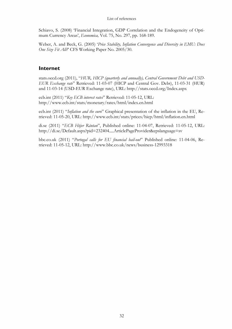
List of references

32

Schiavo, S. (2008) ‘Financial Integration, GDP Correlation and the Endogeneity of Opti-mum Currency Areas’, Economica, Vol. 75, No. 297, pp. 168-189.

Weber, A. and Beck, G. (2005) ‘Price Stability, Inflation Convergence and Diversity in EMU: Does One Size Fit All?’ CFS Working Paper No. 2005/30.

Internet

stats.oecd.org (2011), “HUR, HICP (quarterly and annually), Central Government Debt and USD-EUR Exchange rate” Retrieved: 11-03-07 (HICP and Central Gov. Debt), 11-03-31 (HUR) and 11-03-14 (USD-EUR Exchange rate), URL: http://stats.oecd.org/Index.aspx

ecb.int (2011) “Key ECB interest rates” Retrieved: 11-05-12, URL: http://www.ecb.int/stats/monetary/rates/html/index.en.html

ecb.int (2011) “Inflation and the euro” Graphical presentation of the inflation in the EU, Re-trieved: 11-05-20, URL: http://www.ecb.int/stats/prices/hicp/html/inflation.en.html

di.se (2011) “ECB Höjer Räntan”, Published online: 11-04-07, Retrieved: 11-05-12, URL: http://di.se/Default.aspx?pid=232404__ArticlePageProvider&epslanguage=sv

bbc.co.uk (2011) “Portugal calls for EU financial bail-out” Published online: 11-04-06, Re-trieved: 11-05-12, URL: http://www.bbc.co.uk/news/business-12993318

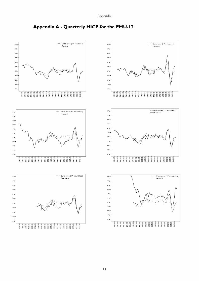
Appendix

33

Appendix A - Quarterly HICP for the EMU-12

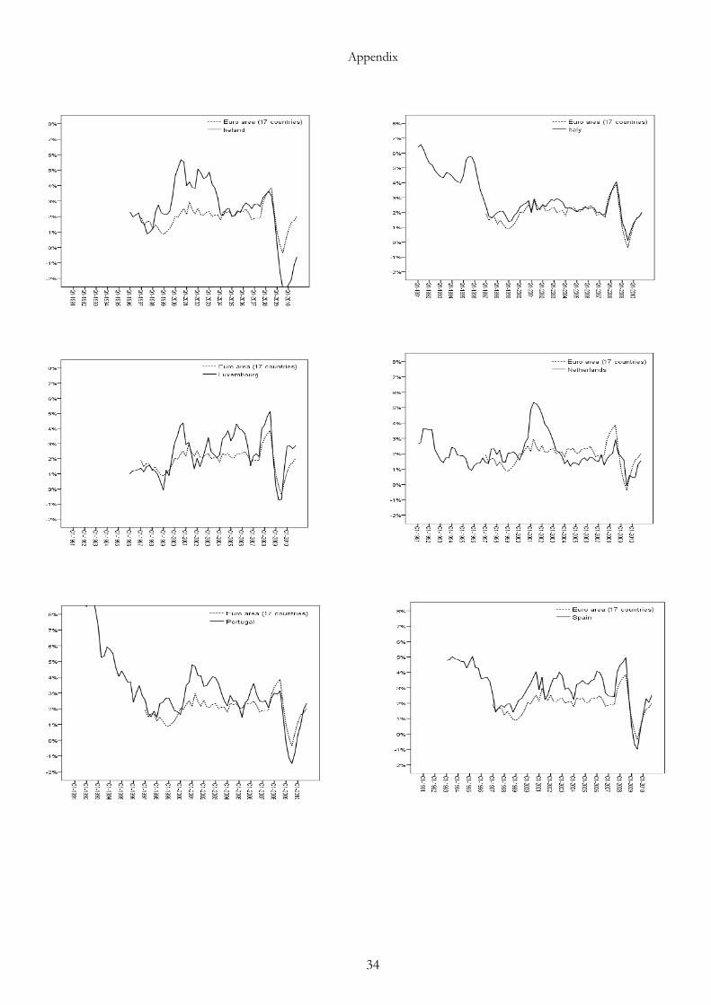
Appendix

34

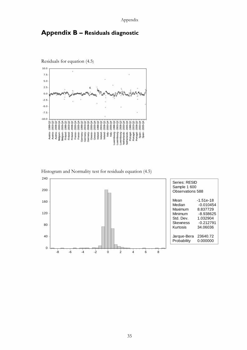
Appendix

35

Appendix B – Residuals diagnostic

Residuals for equation (4.5)

Histogram and Normality test for residuals equation (4.5)

-10.0

-7.5

-5.0

-2.5

0.0

2.5

5.0

7.5

10.0

Aus

tria

- 1

998-

Q2

Aus

tria

- 2

003-

Q2

Aus

tria

- 2

008-

Q2

Bel

gium

- 2

000-

Q4

Bel

gium

- 2

005-

Q4

Fin

land

- 1

998-

Q2

Fin

land

- 2

003-

Q2

Fin

land

- 2

008-

Q2

Fra

nce

- 20

00-Q

4Fra

nce

- 20

05-Q

4G

erm

any

- 19

98-Q

2G

erm

any

- 20

03-Q

2G

erm

any

- 20

08-Q

2G

reec

e -

2000

-Q4

Gre

ece

- 20

05-Q

4Irel

and

- 19

98-Q

2Irel

and

- 20

03-Q

2Irel

and

- 20

08-Q

2It

aly

- 20

00-Q

4It

aly

- 20

05-Q

4Lu

xem

bour

g - 19

98-Q

2Lu

xem

bour

g - 20

03-Q

2Lu

xem

bour

g - 20

08-Q

2N

ethe

rland

s -

2000

-Q4

Net

herla

nds

- 20

05-Q

4P

ortu

gal -

199

8-Q

2P

ortu

gal -

200

3-Q

2P

ortu

gal -

200

8-Q

2S

pain

- 2

000-

Q4

Spa

in -

200

5-Q

4

0

40

80

120

160

200

240

-8 -6 -4 -2 0 2 4 6 8

Series: RESIDSample 1 600Observations 588

Mean -1.51e-18Median -0.010454Maximum 8.837729Minimum -8.938625Std. Dev. 1.032904Skewness -0.212791Kurtosis 34.06036

Jarque-Bera 23640.72Probability 0.000000

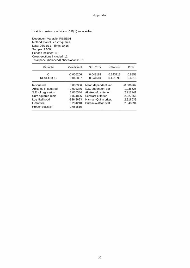
Appendix

36

Test for autocorrelation AR(1) in residual Dependent Variable: RESID01 Method: Panel Least Squares Date: 05/11/11 Time: 10:16 Sample: 1 600 Periods included: 48 Cross-sections included: 12 Total panel (balanced) observations: 576

Variable Coefficient Std. Error t-Statistic Prob. C -0.006206 0.043181 -0.143712 0.8858

RESID01(-1) 0.018837 0.041684 0.451895 0.6515 R-squared 0.000356 Mean dependent var -0.006262

Adjusted R-squared -0.001386 S.D. dependent var 1.035626 S.E. of regression 1.036344 Akaike info criterion 2.912741 Sum squared resid 616.4805 Schwarz criterion 2.927866 Log likelihood -836.8693 Hannan-Quinn criter. 2.918639 F-statistic 0.204210 Durbin-Watson stat 2.048094 Prob(F-statistic) 0.651515

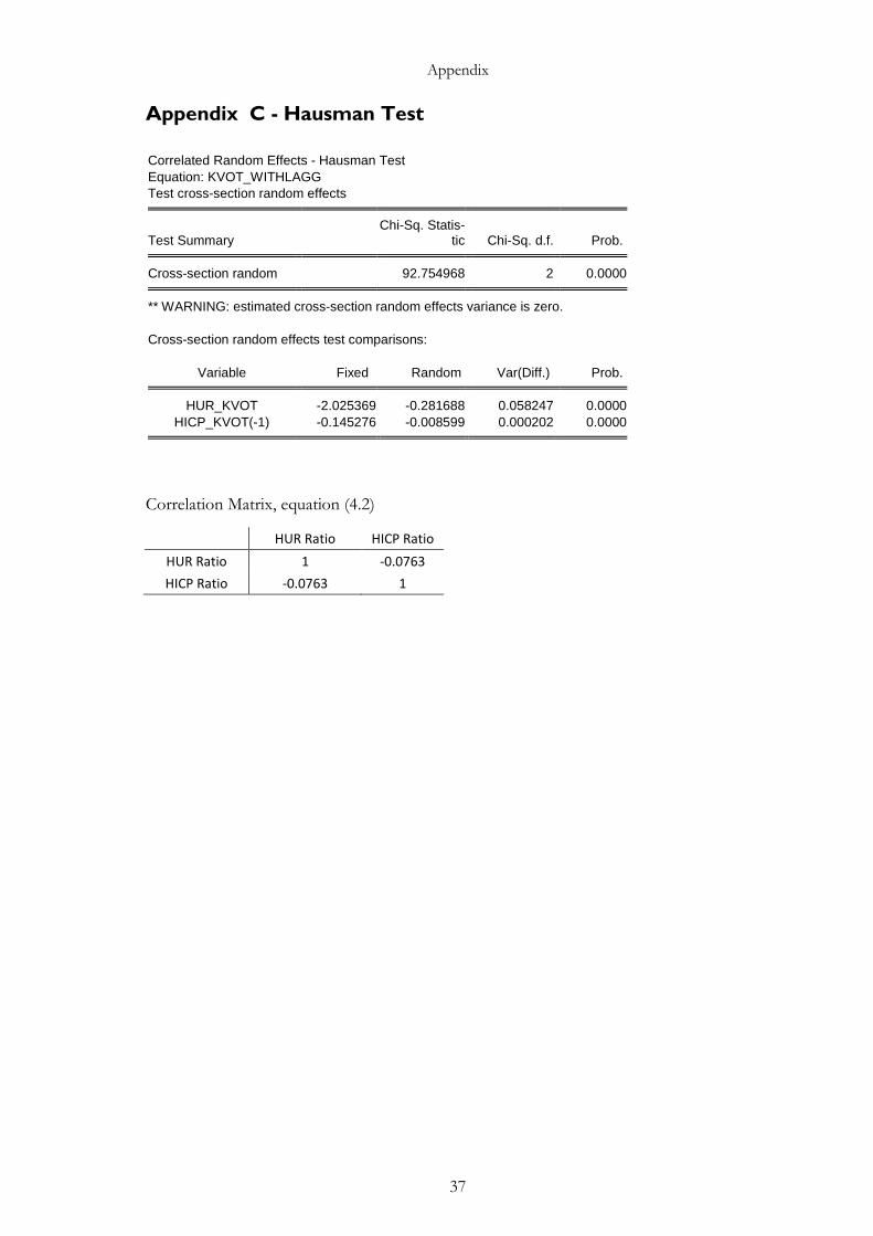
Appendix

37

Appendix C - Hausman Test

Correlated Random Effects - Hausman Test Equation: KVOT_WITHLAGG Test cross-section random effects

Test Summary Chi-Sq. Statis-

tic Chi-Sq. d.f. Prob. Cross-section random 92.754968 2 0.0000 ** WARNING: estimated cross-section random effects variance is zero.

Cross-section random effects test comparisons:

Variable Fixed Random Var(Diff.) Prob. HUR_KVOT -2.025369 -0.281688 0.058247 0.0000

HICP_KVOT(-1) -0.145276 -0.008599 0.000202 0.0000

Correlation Matrix, equation (4.2)

HUR Ratio HICP Ratio

HUR Ratio 1 -0.0763

HICP Ratio -0.0763 1

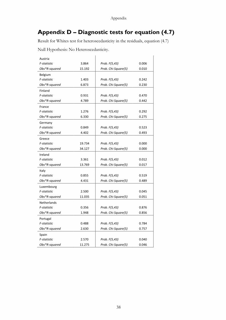
Appendix

38

Appendix D – Diagnostic tests for equation (4.7)

Result for Whites test for heteroscedasticity in the residuals, equation (4.7)

Null Hypothesis: No Heteroscedasticity.

Austria

F-statistic 3.864 Prob. F(5,43) 0.006

Obs*R-squared 15.192 Prob. Chi-Square(5) 0.010

Belgium

F-statistic 1.403 Prob. F(5,43) 0.242

Obs*R-squared 6.873 Prob. Chi-Square(5) 0.230

Finland

F-statistic 0.931 Prob. F(5,43) 0.470

Obs*R-squared 4.789 Prob. Chi-Square(5) 0.442

France

F-statistic 1.276 Prob. F(5,43) 0.292

Obs*R-squared 6.330 Prob. Chi-Square(5) 0.275

Germany

F-statistic 0.849 Prob. F(5,43) 0.523

Obs*R-squared 4.402 Prob. Chi-Square(5) 0.493

Greece

F-statistic 19.734 Prob. F(5,43) 0.000

Obs*R-squared 34.127 Prob. Chi-Square(5) 0.000

Ireland

F-statistic 3.361 Prob. F(5,43) 0.012

Obs*R-squared 13.769 Prob. Chi-Square(5) 0.017

Italy

F-statistic 0.855 Prob. F(5,43) 0.519

Obs*R-squared 4.431 Prob. Chi-Square(5) 0.489

Luxembourg

F-statistic 2.500 Prob. F(5,43) 0.045

Obs*R-squared 11.035 Prob. Chi-Square(5) 0.051

Netherlands

F-statistic 0.356 Prob. F(5,43) 0.876

Obs*R-squared 1.948 Prob. Chi-Square(5) 0.856

Portugal

F-statistic 0.488 Prob. F(5,43) 0.784

Obs*R-squared 2.630 Prob. Chi-Square(5) 0.757

Spain

F-statistic 2.570 Prob. F(5,43) 0.040

Obs*R-squared 11.275 Prob. Chi-Square(5) 0.046

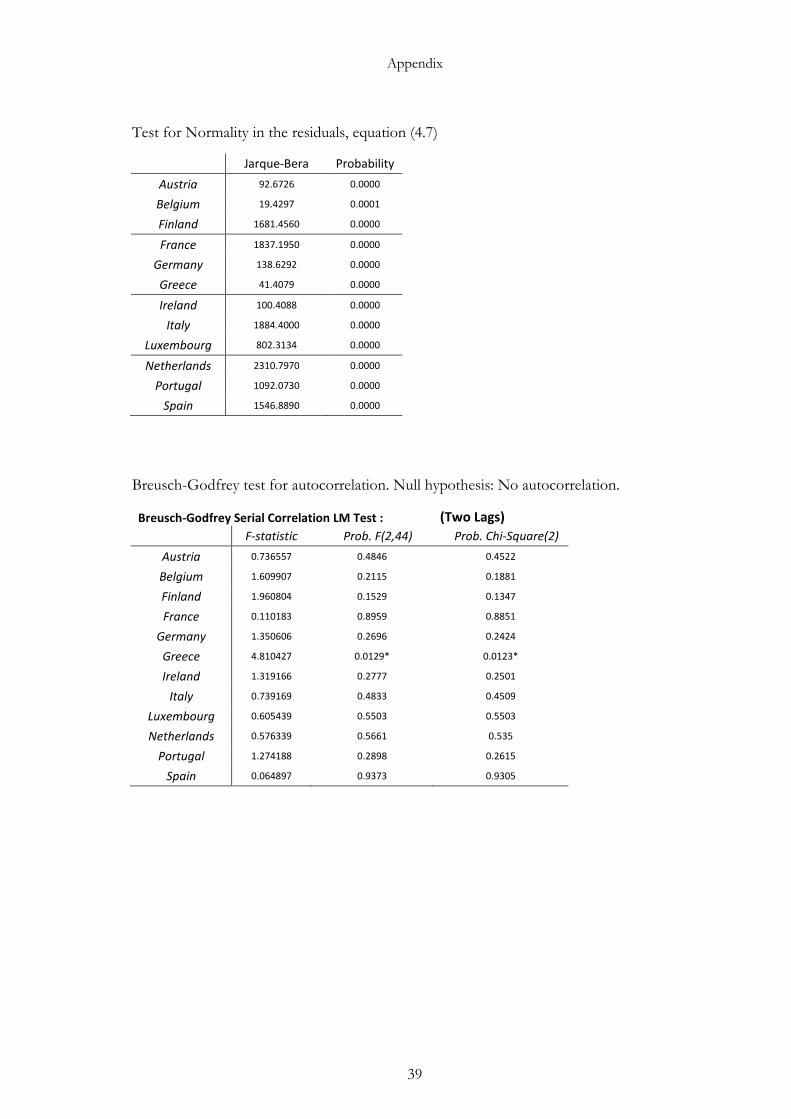
Appendix

39

Test for Normality in the residuals, equation (4.7)

Jarque-Bera Probability

Austria 92.6726 0.0000

Belgium 19.4297 0.0001

Finland 1681.4560 0.0000

France 1837.1950 0.0000

Germany 138.6292 0.0000

Greece 41.4079 0.0000

Ireland 100.4088 0.0000

Italy 1884.4000 0.0000

Luxembourg 802.3134 0.0000

Netherlands 2310.7970 0.0000

Portugal 1092.0730 0.0000

Spain 1546.8890 0.0000

Breusch-Godfrey test for autocorrelation. Null hypothesis: No autocorrelation.

Breusch-Godfrey Serial Correlation LM Test : (Two Lags)

F-statistic Prob. F(2,44) Prob. Chi-Square(2)

Austria 0.736557 0.4846 0.4522

Belgium 1.609907 0.2115 0.1881

Finland 1.960804 0.1529 0.1347

France 0.110183 0.8959 0.8851

Germany 1.350606 0.2696 0.2424

Greece 4.810427 0.0129* 0.0123*

Ireland 1.319166 0.2777 0.2501

Italy 0.739169 0.4833 0.4509

Luxembourg 0.605439 0.5503 0.5503

Netherlands 0.576339 0.5661 0.535

Portugal 1.274188 0.2898 0.2615

Spain 0.064897 0.9373 0.9305