diversity in cognitive ability enlarges mispricing in
TRANSCRIPT
HAL Id: halshs-01202088https://halshs.archives-ouvertes.fr/halshs-01202088v2
Preprint submitted on 24 Oct 2017
HAL is a multi-disciplinary open accessarchive for the deposit and dissemination of sci-entific research documents, whether they are pub-lished or not. The documents may come fromteaching and research institutions in France orabroad, or from public or private research centers.
L’archive ouverte pluridisciplinaire HAL, estdestinée au dépôt et à la diffusion de documentsscientifiques de niveau recherche, publiés ou non,émanant des établissements d’enseignement et derecherche français ou étrangers, des laboratoirespublics ou privés.
Diversity in Cognitive Ability Enlarges Mispricing inExperimental Asset Markets
Nobuyuki Hanaki, Eizo Akiyama, Yukihiko Funaki, Ryuichiro Ishikawa
To cite this version:Nobuyuki Hanaki, Eizo Akiyama, Yukihiko Funaki, Ryuichiro Ishikawa. Diversity in Cognitive AbilityEnlarges Mispricing in Experimental Asset Markets. 2017. �halshs-01202088v2�
Diversity in Cognitive Ability enlArges MispriCing in experiMentAl Asset MArkets
Documents de travail GREDEG GREDEG Working Papers Series
Nobuyuki HanakiEizo AkiyamaYukihiko FunakiRyuichiro Ishikawa
GREDEG WP No. 2017-08https://ideas.repec.org/s/gre/wpaper.html
Les opinions exprimées dans la série des Documents de travail GREDEG sont celles des auteurs et ne reflèlent pas nécessairement celles de l’institution. Les documents n’ont pas été soumis à un rapport formel et sont donc inclus dans cette série pour obtenir des commentaires et encourager la discussion. Les droits sur les documents appartiennent aux auteurs.
The views expressed in the GREDEG Working Paper Series are those of the author(s) and do not necessarily reflect those of the institution. The Working Papers have not undergone formal review and approval. Such papers are included in this series to elicit feedback and to encourage debate. Copyright belongs to the author(s).
Diversity in cognitive ability and mispricing in
experimental asset markets∗
Nobuyuki Hanaki† Eizo Akiyama‡ Yukihiko Funaki§ Ryuichiro Ishikawa¶
GREDEG Working Paper No. 2017–08
Abstract
Does diversity of cognitive ability among market participants increase mispricing?Does common knowledge of heterogeneity in relation to cognitive ability of marketparticipants further increase mispricing? We investigated these questions by measur-ing subjects’ cognitive ability and categorizing those above median ability as type ‘H’and those below median ability as type ‘L’. We then constructed three market types,each containing six traders: 6H, 6L, and 3H3L. Subjects were informed of their owncognitive type and, depending on the treatment, that of the others in their market.We found that heterogeneous markets (3H3L) generated significantly larger mispricingthan homogeneous markets (6H or 6L) regardless of whether subjects were informedabout the cognitive type of others in their market. Thus, diversity of cognitive abil-ity among market participants increased mispricing. However, common knowledge ofheterogeneity or homogeneity in the market did not have a significant additional effect.
Keywords: Cognitive ability, Heterogeneity, Mispricing, Experimental asset markets
JEL Code: C90, D84
∗This is a major revision (involving a completely new set of experiments) of the GREDEG Working Paper2015-29 entitled “Diversity in Cognitive Ability Enlarges Mispricing.” Misaki Miyaji, Ayano Nakagawa, andMakoto Soga provided invaluable help in organizing the experiments. Comments and suggestions from TeBao, Jurgen Huber, Daniel Kleinlercher, Fabrice Le Lec, Charles Noussair, Michael Razen, Eko Riyanto,Thomas Stockl, and seminar participants at CREM, Edinburgh, Glasgow, GRIPS, GREDEG, Hitotsubashi,Hokkaido, Innsbruck, Keio, Osaka, Waseda, Ritsumeikan, and Nanyang Technological University, as wellas participants at SEF 2015 (Nijmegen), CEF 2016 (Bordeaux), FUR 2016 (Warwick), and SEF NorthAmerica 2016 (Tuscan) are gratefully acknowledged. Jeremy Mercer performed an excellent proofread. Thisproject is partly financed by a JSPS-ANR bilateral research grant “BECOA” (ANR-11-FRJA-0002), ORA-Plus research project “BEAM” (ANR-15-ORAR-0004), financial aid from the Japan Center for EconomicResearch, and financial aid from the Japan Securities Scholarship Foundation. A part of this work wasconducted when Hanaki was affiliated with Aix-Marseille Universite (Aix-Marseille School of Economics).Hanaki thanks Aix-Marseille School of Economics for their support. The experiments reported in this paperhave been approved by the Institutional Review Board of the Faculty of Engineering, Information andSystems, University of Tsukuba (No. 2012R25).†Universite Cote d’Azur, CNRS, GREDEG. Corresponding author. GREDEG, 250 rue Albert Einstein,
06560 Valbonne, France. E-mail: [email protected]‡Faculty of Engineering, Information and Systems, University of Tsukuba. E-mail: [email protected]§School of Political Science and Economics, Waseda University. E-mail: [email protected]¶School of International Liberal Studies, Waseda University. E-mail: [email protected]
1
1 Introduction
Economic bubbles are often characterized by market euphoria and an inflow of new and
possibly naıve investors (Kindleberger and Aliber, 2005). Indeed, Lopez (2015) reports that
a non-negligible fraction of new investors in China’s stock market is unable to read, and for
a majority of these new investors, junior high school is the highest level of education they
have completed. Such an inflow of new investors can amplify heterogeneity among market
participants regarding their belief about future prices of the asset being traded, as well as
their naivety in terms of financial knowledge and trading behavior, and thus may increase
mispricing, as noted by Xiong and Yu (2011) in their study of “bubbles” in a subset of
China’s warrant market.
Furthermore, several theoretical works (Allen and Gale, 1992; Aggarwal and Wu, 2006;
Allen et al., 2006) build upon this idea and show how heterogeneity in terms of (strategic)
sophistication among traders can lead to significant mispricing. Allen and Gale (1992), for
example, show that sophisticated strategic traders try to generate an initial upward price
trend to influence the belief of naıve trend followers and later profit from their naıvete.
Recent experimental studies have demonstrated the relationship between the cognitive
abilities of subjects and mispricing in asset-market experiments a la Smith et al. (1988).1
Breaban and Noussair (2015) and Cueva and Rustichini (2015) show that the average cog-
nitive skill of subjects in the market is negatively correlated with the degree of mispricing
observed in the market. Cognitive skills are measured by the Cognitive Reflection Test
(CRT, Frederick, 2005) in the former and by the Raven’s progressive matrices (RPM) test
(see Raven, 2008, for an overview) and Race to X game (Gneezy et al., 2010; Dufwenberg
et al., 2010) in the latter. Corgnet et al. (2015) and Cueva and Rustichini (2015) demon-
strate that subjects with higher cognitive skills earn more than their counterparts with lower
cognitive skills.
These experimental findings are in line with findings from empirical studies based on
large-scale surveys that tend to report that people with high cognitive skills make better
financial decisions (see, for example, Korniotis and Kumar, 2010, for a survey of the empirical
1See Palan (2013) and Powell and Shestakova (2016) for recent surveys of the literature. However, thebody of literature is expanding very quickly, with many new papers being presented each year at the annualmeeting of the Society of Experimental Finance. See http://www.experimentalfinance.org/ for a list ofpapers presented at recent meetings.
2
literature).
However, the effect of interactions among traders with varying degrees of strategic so-
phistication has not been explicitly investigated to any great extent, either empirically or
experimentally. The abovementioned experimental studies only relate cognitive skills and
market outcomes ex post, and thus do not use cognitive skills as an experimental variable.2
An exception is the study by Bosch-Rosa et al. (2015), who investigate how the average
cognitive ability of market participants influences mispricing in an experimental market
by creating markets based explicitly on the subjects’ cognitive abilities measured ex ante.
Bosch-Rosa et al. (2015) first conduct an experimental session consisting of the CRT, guess-
ing games, and multiple rounds of the Race to 60 game to measure and create a composite
index of the cognitive abilities of their subjects. Then, they select subjects from the top
30% (“high sophistication”) and bottom 30% (“low sophistication”) of their subject pool ac-
cording to the index and conduct an asset-market experiment using markets consisting only
of high-sophistication subjects or those consisting only of low-sophistication subjects. They
report significant mispricing in the markets consisting only of low-sophistication subjects
but almost no mispricing in those consisting only of high-sophistication subjects.
These experimental and empirical studies lead us to speculate that the mispricing ob-
served in both experimental and real financial markets is primarily due to bad decision-
making by naıve market participants, rather than by interactions (both strategic and non-
strategic) among traders with varying degrees of cognitive sophistication. However, two
recent experimental studies by Cheung et al. (2014) and Akiyama et al. (2015) have demon-
strated that this might not be the whole story.
2There is an increasing number of experimental studies on games and individual decisions that usecognitive skills as an experimental variable. For example, in game theoretic settings, Gill and Prowse (2016)study a three-player p-beauty contest game by creating three types of groups based on the subjects’ relativecognitive ability: an all-high-cognitive-ability group, an all-low-cognitive-ability group, and a mixed group.They find that subjects with higher cognitive ability are faster at learning to choose numbers close to theNash equilibrium, and thus earn more. They also find that those with high cognitive ability respond tothe cognitive ability of their counterparts, while those with low cognitive ability do not. Another recentgame theoretic work is that of Proto et al. (2016). They study the evolution of cooperation in repeatedgames while varying the cognitive ability of groups and find that, although the initial levels of cooperationare similar, groups with high cognitive ability learn to achieve high or full cooperation, while cooperationdeclines in groups with low cognitive ability. Regarding studies on individual decision-making, Dohmen et al.(2010), in their study using a German sample, find that subjects with higher cognitive ability take morecalculated risks and are more patient. Oechssler et al. (2009) study the relationships between CRT scoresand various behavioral biases such as the conjunction fallacy and conservatism in updating probabilities, aswell as time and risk preferences. They find similar relationships between CRT scores and risk and timepreferences to those found by Dohmen et al. (2010), as well as a negative correlation between CRT scoresand the incidence of the two biases.
3
Cheung et al. (2014) investigate the effect of a lack of common knowledge in terms of
subjects’ understanding of the fundamental value (FV) of the asset being traded. They
train some of their subjects extensively about the FV of the asset before the experiment,
and then compare the degree of mispricing in three types of markets: (1) everyone is trained
and knows that everyone else is also trained, (2) everyone is trained but no one knows that
everyone else is also trained, and (3) no one is trained. The results show that the degree
of mispricing is small only when everyone is trained and it is common knowledge. When it
is not common knowledge that everyone is trained, the mispricing is as large as that in the
market where no one is trained.
Akiyama et al. (2015) investigate how the presence of uncertainty about the behavior of
others in the market influences long-term price forecasts by comparing the price forecasts in
two market environments: one in which one subject interacts with computer traders with
known behavior, and another in which subjects interact among themselves. They find that
the subjects’ initial long-term forecasts deviate further from FV in the former case than
in the latter. Furthermore, subjects with a perfect CRT score react more strongly to the
presence of uncertainty about the behavior of others in the market (where they interact
with other subjects) than those with lower CRT scores by forecasting future prices that
deviate further from the FV compared with the market without such uncertainty (where
they interact with computer traders with known behavior).
Because diversity (or heterogeneity) in cognitive ability among market participants can
be an important source of heterogeneous belief about future prices, as well as behavioral
uncertainty in cases where the heterogeneity is common knowledge, these two experimental
studies hint at the possibility that such diversity can indeed amplify the mispricing of the
asset being traded. Therefore, in this paper, we investigate whether heterogeneity in cognitive
ability among market participants increases mispricing. In addressing this question, we also
investigate the relationship between the average cognitive ability of market participants and
the degree of mispricing. Furthermore, we ask whether common knowledge of heterogeneity
(or homogeneity) in cognitive ability among market participants further increases mispricing.
The latter question is motivated by the theoretical literature on strategic manipulation cited
above. We conjecture that knowing that naive traders are present in the market creates
an opportunity for more sophisticated traders to manipulate prices, and thus increases
4
mispricing.
We approach these research questions by first measuring subjects’ cognitive ability using
a part of the advanced version of the RPM test,3 and then grouping subjects based on
their relative RPM test scores within an experimental session. That is, subjects with an
RPM score above the median are labeled H types and those with an RPM score below the
median are labeled L types. We consider three types of markets: those consisting solely
of H types, those consisting solely of L types, and those consisting of equal numbers of H
and L types. By comparing the outcomes of these three types of markets, we investigate
the influence not only of the average cognitive ability of market participants, but also of
diversity in cognitive ability on market outcomes. Furthermore, we investigate the impact
of subjects being informed about the composition of the market participants on market out-
comes by conducting experiments wherein the subjects either are or are not informed about
the composition of the market in which they participate. Our main aim is to investigate the
effect of heterogeneity of cognitive ability among market participants by creating markets
that mix both high- and low-sophistication subjects, which is an aspect that Bosch-Rosa
et al. (2015) do not address.
We found that heterogenous markets, i.e., markets consisting of an equal number of
H- and L-type subjects, showed a greater degree of mispricing than the two homogeneous
markets, i.e., those consisting solely of either H- or L-type subjects, regardless of whether the
composition of the market was ex ante known or otherwise. Our results showed that not only
the average cognitive ability of market participants but also their heterogeneity, regardless
of whether that heterogeneity is ex ante known or otherwise, increases mispricing. However,
we did not find any significant difference in terms of mispricing between treatments with and
without subjects being ex ante informed about the composition of the market. Thus, we did
not observe any significant additional effect of common knowledge of cognitive heterogeneity
on mispricing beyond the effect of the existence of cognitive heterogeneity.
3The RPM test measures what is called “fluid intelligence,” that is, “the capacity to think logically,analyze and solve novel problems, independent of background knowledge” (Mullainathan and Shafir, 2013,p. 48) and its score has been shown to be correlated to the degree of strategic sophistication, which ismeasured in terms of the number of wins in Race to 5, 10, and 15 games (Carpenter et al., 2013) or thedeviation from the equilibrium in a three-player p-beauty contest game (Gill and Prowse, 2016). “Fluidintelligence” should be distinguished from what is called “executive control.” The latter is the ability tocontrol one’s impulsive behavior or responses. Thus, the CRT score can be interpreted as a measure of one’sexecutive control, not their fluid intelligence.
5

2 Experiment
In each session involving 24 subjects, we first asked the subjects to complete a part of the
advanced version of the RPM test (24 questions to be answered in 15 minutes).4 We did
not tell our subjects why they were required to complete the test (which we termed a quiz
during the experiment), nor what kind of experiments would follow. Thus, our subjects were
unaware that their scores on the RPM test would be used to place them into different groups
in an asset market experiment. In accordance with standard practice in administering the
RPM test, we did not offer any monetary incentives to our subjects for answering as many
questions as possible correctly.
Following the RPM test, we divided our subjects into two types based on their scores
on the RPM test. Those above the median score were termed ‘H type’ and those below
the median score were termed ‘L type’. We then created three versions of a 20-period call
asset market with six traders in each market: in version one, all six traders were H type (6H
markets); in version two, all six traders were L type (6L markets); and in version three, there
were equal numbers of H and L types (3H3L markets). In one experimental session using
our 24 subjects, we created two 6H markets and two 6L markets, and in another session,
we created four 3H3L markets.5 In all of our treatments, we informed our subjects of their
own type (H or L), but not how many quiz questions they had answered correctly.
To investigate the effect of (1) the composition of the market participants (in terms
of their relative cognitive ability) and (2) the fact that the composition was known to the
market participants, we considered two information treatments. In half of our treatments, we
did not inform our subjects of the composition of their market (unknown composition), while
in the other half, we informed them of the composition (known composition). Therefore, in
the unknown composition treatment, subjects were only informed of their own type, H or
L, but not the type of the five other traders in their market.6 In the known composition
4The full advanced version of the RPM test consists of 48 questions to be answered in 30−40 minutes.We used all of the odd-numbered questions from the full test, retaining the original order to ensure that thequestions became progressively more difficult.
5Groups were created according to the rankings on the RPM test of the participants in that session. Inthe 24-subject 6H and 6L session, the first 6H market consisted of subjects with rankings of {1, 3, 5, 7, 9, 11}and the second consisted of subjects with rankings of {2, 4, 6, 8, 10, 12}, while the first 6L market consistedof subjects with rankings of {13, 15, 17, 19, 21, 23} and the second consisted of subjects with rankings of{14, 16, 18, 20, 22, 24}. For the 3H3L markets, we established four markets that consisted of subjects withrankings of {1, 5, 9, 13, 17, 21}, {2, 6, 10, 14, 18, 22}, {3, 7, 11, 15, 19, 23}, and {4, 8, 12, 16, 20, 24}. In caseswhere subjects had identical scores, rankings were assigned randomly.
6We informed our subjects in the unknown composition treatment as follows. At the beginning of the
6
treatment, if an H-type subject was in a 6H market, s/he was informed that s/he was H
type and all of the other five traders in the market were also H type. If an H-type subject
was in a 3H3L market, s/he was informed that s/he was H type and that the other five
traders consisted of two H-type traders and three L-type traders. Similarly, if an L-type
subject was in a 6L market, s/he was informed that s/he was L type and all of the other
five traders in the market were also L type.7
In all of the markets, traders are initially given four units of the asset and 1040 experi-
mental currency units (ECUs), which they can use to trade over 20 periods. Each unit of the
asset pays a dividend of 12 ECUs at the end of each period, which is added to traders’ cash
holdings and can be used for trading in future periods. After the final dividend payment
at the end of period 20, all of the assets lose their value. Under these conditions, the FV
of a unit of the asset during period t (t = 1, 2, ..., T ), FVt, is the sum of the remaining
dividend payments, that is, FVt = 12(21− t). For example, a unit of the asset has an initial
value of 240 ECUs. Thus, the value of the initial endowment is 2000 ECUs for all of the
market participants (1040 ECUs in initial currency plus 960 ECUs for the four units of the
asset). We have eliminated uncertainty in dividend payments to minimize the presence of
uncertainty beyond that caused by the behavior of market participants. Even with fixed
and known dividend payments, mispricing has been observed in these markets (Porter and
Smith, 1995; Akiyama et al., 2014, 2015).
We employ a call market mechanism, as in van Boening et al. (1993); Haruvy et al.
(2007); Akiyama et al. (2014, 2015), instead of a continuous double auction as used in many
asset-market experiment, we told them that “You have been divided into the top 12 scorers and the bottom12 scorers out of the 24 people who completed the quiz. Before starting the game, you will know what yourrank is, i.e., the top 12 or the bottom 12. The 24 people in the room are divided into four groups of six.”We displayed each subject’s type (H or L) on the first screen presented to them during the asset-marketexperiment.
7More specifically, we informed subjects in the known composition treatment as follows. (1) At thebeginning of the asset-market experiment, we stated, in the 6H and 6L treatments, that “You have beendivided into the top 12 scorers and the bottom 12 scorers out of the 24 people who completed the quiz.Before starting the game, you will know what your rank is, i.e., the top 12 or the bottom 12. The 24 peoplein the room have been divided into four groups of six. Two of the four groups consist of the top 12 scorersand the other two groups consist of the bottom 12 scorers.” In the case of the 3H3L markets, the lastsentence of the statement read, “Each of the four groups consists of three top scorers and three bottomscorers.” (2) At the end of the instruction, we repeated the same information. In the 6H or 6L treatments,we advised subjects that “There are six people in each market. All of those people are in this room. Eachgroup consists entirely of either the top scorers or the bottom scorers in the quiz. Your ranking, in either thetop or the bottom half, is shown on the first screen.” In the case of the 3H3L treatment, the third sentencewas “Each group consists of three people who scored in the top half and three who scored in the bottomhalf in the quiz.” See the Appendix for an English translation of the instructions, as well as examples of thefirst screen displayed in the asset-market experiment, in which the subjects’ type and group compositionwere displayed.
7
other studies. In our call market, in each period, each trader can submit at most one buy
order and one sell order.8 An order consists of a pair of values: a price and a quantity.
When submitting a buy order in period t, trader i must specify the maximum price, bit,
at which s/he is willing to buy a unit of the asset, and the maximum quantity, dit, s/he is
willing to buy at that price. In the same manner, when submitting a sell order in period t,
trader i must specify the minimum price, ait, at which s/he is willing to sell a unit of the
asset, and the maximum quantity, sit, s/he is willing to sell at that price. We attach three
constraints: the admissible price range, a budget constraint, and the relationship between
bit and ait in the case where a subject submits both buy and sell orders. The admissible
price range is set so that when dit ≥ 1 (sit ≥ 1), bit (ait) must be an integer between 1 and
2000, i.e., bit ∈ {1, 2, ..., 2000} (ait ∈ {1, 2, ..., 2000}). The budget constraint simply means
that neither borrowing of cash nor short selling of an asset is allowed.9 The final constraint
is that when a trader is submitting both buy and sell orders, i.e., dit ≥ 1 and sit ≥ 1, the
maximum buying price must not be greater than the minimum selling price, i.e., ait ≥ bit.
Once all of the traders in the market have submitted their orders, the price that clears the
market is calculated,10 and all transactions are processed at that price among traders who
submitted a maximum buying price no less than, or a minimum selling price no greater
than, the market clearing price.11
The entire experiment was computerized using z-Tree (Fischbacher, 2007). Each session
lasted for about one and a half hours, including a post-experiment questionnaire. We also
administered the CRT as a part of the post-experiment questionnaire, with no monetary
incentive for correct answers. On average, subjects earned 3000 yen (≈ 22 euros at the
average exchange rate prevailing during the period of the experiment), including a 1000-yen
participation fee. See the Appendix for an English translation of the instructions.
8Of course, a trader can choose not to submit any orders by specifying zero as the quantities to buy andsell. We imposed a 60-second, non-binding time limit for submitting orders. When the time limit is reached,the subjects are instructed via a flashing message in the upper right corner of their screen to submit theirorders as soon as possible.
9Thus, the budget constraint implies (i) dit × bit ≤ cash holding at the beginning of the period t, and (ii)sit ≤ units of asset on hand at the beginning of the period t.
10Following the previous experiments (Haruvy et al., 2007; Akiyama et al., 2014, 2015), when there areseveral such prices, the lowest one is chosen as the market clearing price. This is important to ensure thatthe price does not rise in the absence of transactions at the market clearing price.
11Any ties among the last accepted buy or sell orders are resolved randomly. It is possible that notransaction will take place given the computed market clearing price.
8
Table 1: Summary of treatments
Treatment No. of subjects No. of marketsUnknown composition, 6H 48 8Unknown composition, 6L 48 8
Unknown composition, 3H3L 48 8Known composition, 6H 72 12Known composition, 6L 72 12
Known composition, 3H3L 72 12
3 Results
The experiment was conducted at Waseda University in Tokyo, Japan between November
2014 and July 2016. A total of 360 subjects participated; 144 subjects in unknown compo-
sition treatments, of which 96 participated in 6H/6L sessions and 48 participated in 3H3L
sessions, and 216 subjects in known composition treatments, of which 144 participated in
6H/6L sessions and 72 participated in 3H3L sessions. Subjects were recruited from the main
university campus via emails and flyers. These subjects had never participated in a similar
experiment before, and each subject only participated in one session. Therefore, we had
eight markets for the unknown composition treatment and 12 markets for the known compo-
sition treatment, each market comprising six subjects. Table 1 summarizes the treatments
and the number of subjects participating in each treatment.
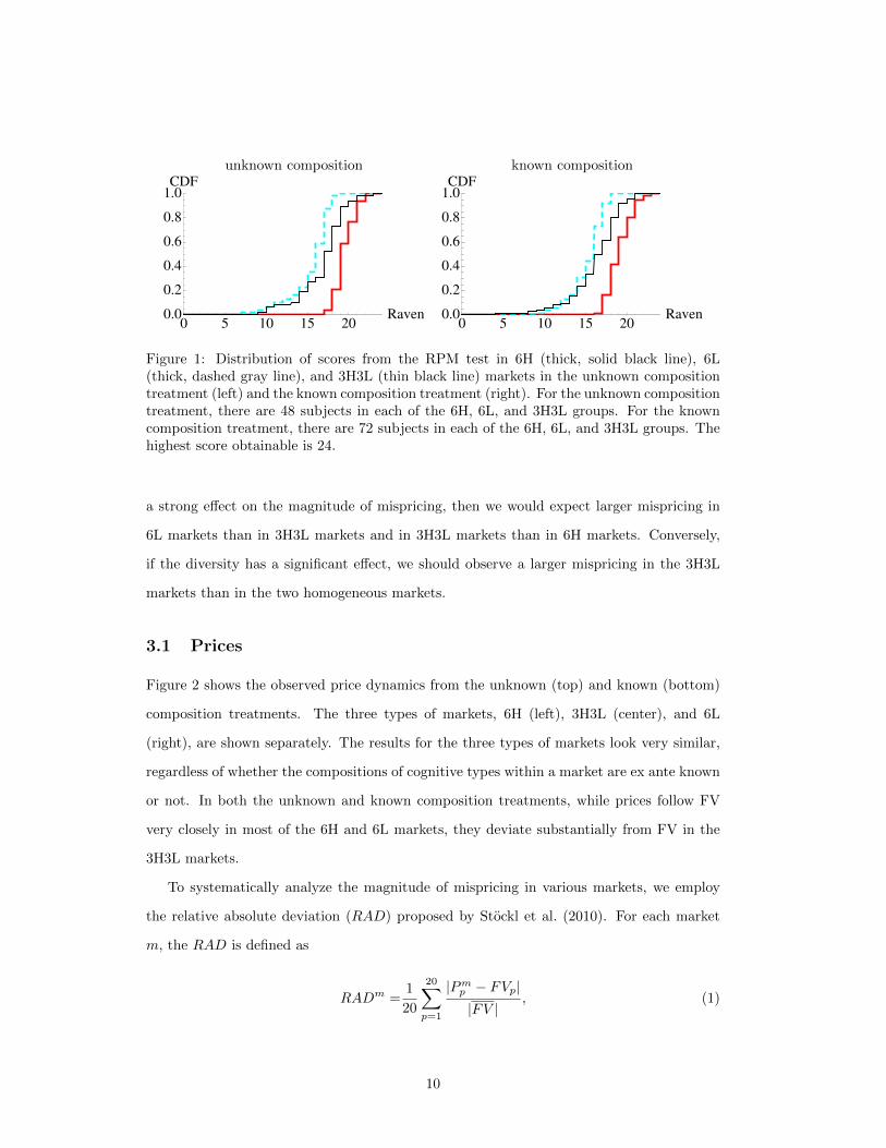
Figure 1 shows the empirical cumulative distributions of the scores from the RPM test
(RPM scores) for the participants in the unknown composition (left) and known composition
(right) treatments. In each panel, three types of markets are shown separately: 6H (thick,
solid red line), 6L (thick, dashed blue line), and 3H3L (thin black line). By construction,
the empirical cumulative distribution of the RPM scores is in the order 6L, 3H3L, and 6H
from left (lowest) to right (highest). The distribution of RPM scores between unknown
and known composition treatments are not statistically significantly different for each of the
market types (p-values are 0.123 for 6H markets, 0.592 for 6L markets, and 0.22 for 3H3L
markets according to a two-sample permutation test (PT), two-tailed).
The results from the previous studies mentioned in the Introduction suggest a negative
relationship between the average level of cognitive ability among traders and mispricing in
markets. If the diversity (or heterogeneity) of cognitive ability among traders does not have
9
unknown composition known composition
0 5 10 15 20Raven0.0
0.2
0.4
0.6
0.8
1.0CDF
0 5 10 15 20Raven0.0
0.2
0.4
0.6
0.8
1.0CDF
Figure 1: Distribution of scores from the RPM test in 6H (thick, solid black line), 6L(thick, dashed gray line), and 3H3L (thin black line) markets in the unknown compositiontreatment (left) and the known composition treatment (right). For the unknown compositiontreatment, there are 48 subjects in each of the 6H, 6L, and 3H3L groups. For the knowncomposition treatment, there are 72 subjects in each of the 6H, 6L, and 3H3L groups. Thehighest score obtainable is 24.
a strong effect on the magnitude of mispricing, then we would expect larger mispricing in
6L markets than in 3H3L markets and in 3H3L markets than in 6H markets. Conversely,
if the diversity has a significant effect, we should observe a larger mispricing in the 3H3L
markets than in the two homogeneous markets.
3.1 Prices
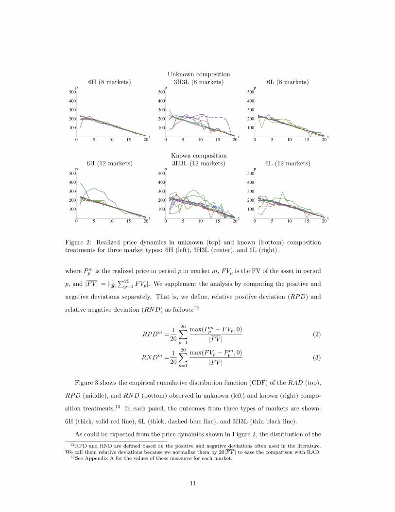
Figure 2 shows the observed price dynamics from the unknown (top) and known (bottom)
composition treatments. The three types of markets, 6H (left), 3H3L (center), and 6L
(right), are shown separately. The results for the three types of markets look very similar,
regardless of whether the compositions of cognitive types within a market are ex ante known
or not. In both the unknown and known composition treatments, while prices follow FV
very closely in most of the 6H and 6L markets, they deviate substantially from FV in the
3H3L markets.
To systematically analyze the magnitude of mispricing in various markets, we employ
the relative absolute deviation (RAD) proposed by Stockl et al. (2010). For each market
m, the RAD is defined as
RADm =1
20
20∑p=1
|Pmp − FVp||FV |
, (1)
10
Unknown composition6H (8 markets) 3H3L (8 markets) 6L (8 markets)
0 5 10 15 20t
100
200
300
400
500P
0 5 10 15 20t
100
200
300
400
500P
0 5 10 15 20t
100
200
300
400
500P
Known composition6H (12 markets) 3H3L (12 markets) 6L (12 markets)
0 5 10 15 20t
100
200
300
400
500P
0 5 10 15 20t
100
200
300
400
500P
0 5 10 15 20t
100
200
300
400
500P
Figure 2: Realized price dynamics in unknown (top) and known (bottom) compositiontreatments for three market types: 6H (left), 3H3L (center), and 6L (right).
where Pmp is the realized price in period p in market m, FVp is the FV of the asset in period
p, and |FV | = | 120∑20
p=1 FVp|. We supplement the analysis by computing the positive and
negative deviations separately. That is, we define, relative positive deviation (RPD) and
relative negative deviation (RND) as follows:12
RPDm =1
20
20∑p=1
max(Pmp − FVp, 0)
|FV |(2)
RNDm =1
20
20∑p=1
max(FVp − Pmp , 0)
|FV |. (3)
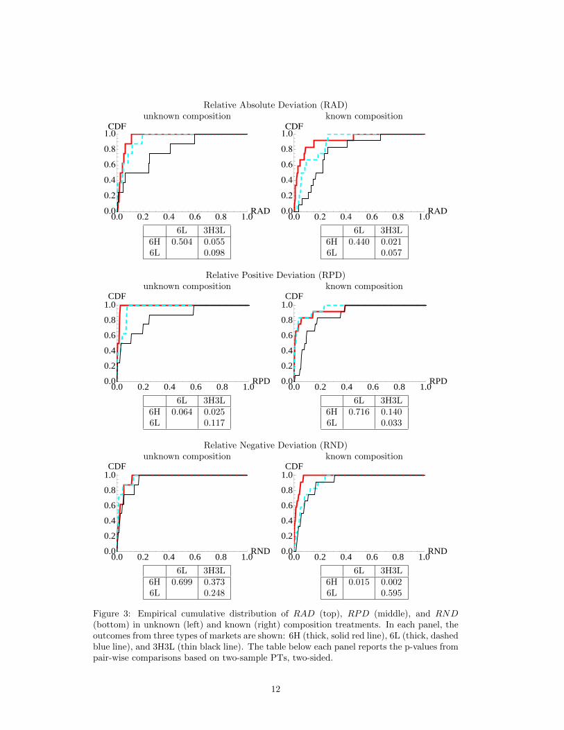
Figure 3 shows the empirical cumulative distribution function (CDF) of the RAD (top),
RPD (middle), and RND (bottom) observed in unknown (left) and known (right) compo-
sition treatments.13 In each panel, the outcomes from three types of markets are shown:
6H (thick, solid red line), 6L (thick, dashed blue line), and 3H3L (thin black line).
As could be expected from the price dynamics shown in Figure 2, the distribution of the
12RPD and RND are defined based on the positive and negative deviations often used in the literature.We call them relative deviations because we normalize them by 20|FV | to ease the comparison with RAD.
13See Appendix A for the values of these measures for each market.
11
Relative Absolute Deviation (RAD)unknown composition known composition
0.0 0.2 0.4 0.6 0.8 1.0RAD0.0
0.2
0.4
0.6
0.8
1.0CDF
0.0 0.2 0.4 0.6 0.8 1.0RAD0.0
0.2
0.4
0.6
0.8
1.0CDF
6L 3H3L6H 0.504 0.0556L 0.098
6L 3H3L6H 0.440 0.0216L 0.057
Relative Positive Deviation (RPD)unknown composition known composition
0.0 0.2 0.4 0.6 0.8 1.0RPD0.0
0.2
0.4
0.6
0.8
1.0CDF
0.0 0.2 0.4 0.6 0.8 1.0RPD0.0
0.2
0.4
0.6
0.8
1.0CDF
6L 3H3L6H 0.064 0.0256L 0.117
6L 3H3L6H 0.716 0.1406L 0.033
Relative Negative Deviation (RND)unknown composition known composition
0.0 0.2 0.4 0.6 0.8 1.0RND0.0
0.2
0.4
0.6
0.8
1.0CDF
0.0 0.2 0.4 0.6 0.8 1.0RND0.0
0.2
0.4
0.6
0.8
1.0CDF
6L 3H3L6H 0.699 0.3736L 0.248
6L 3H3L6H 0.015 0.0026L 0.595
Figure 3: Empirical cumulative distribution of RAD (top), RPD (middle), and RND(bottom) in unknown (left) and known (right) composition treatments. In each panel, theoutcomes from three types of markets are shown: 6H (thick, solid red line), 6L (thick, dashedblue line), and 3H3L (thin black line). The table below each panel reports the p-values frompair-wise comparisons based on two-sample PTs, two-sided.
12
RAD from the 3H3L markets lies to the right of those from the 6H and 6L markets in both
unknown and known composition treatments. The pair-wise comparisons show that the
RAD in the 3H3L markets is significantly greater than those in the 6H and 6L markets (p-
values are 0.055 for 6H vs 3H3L markets and 0.098 for 6L vs 3H3L markets in the unknown
composition treatment, and 0.021 for 6H vs 3H3L markets and 0.057 for 6L vs 3H3L markets
in the known composition treatment, according to two-sample PTs, two-tailed). The RAD
does not differ significantly between the two homogeneous markets, 6H and 6L (p-values are
0.504 and 0.440 for the unknown and known composition treatments, respectively, according
to two-sample PTs, two-tailed).
Similar results are obtained for the RPD, but not for the RND. The RPD from the
3H3L markets lies to the right of those from the 6H and 6L markets in both the known
and unknown composition treatments, although the RPDs are no longer statistically signif-
icantly different between the 3H3L and 6L markets in the unknown composition treatment
or between the 3H3L and 6H markets in the known composition treatment at the 10% level.
The distributions of the RNDs observed in the three types of markets in the unknown com-
position treatment are almost aligned. For the known composition treatment, the RND in
the 6H markets is significantly smaller than that in both the 6L and 3H3L markets. The
distributions of the RNDs in the latter two markets are aligned. This suggests that the
significantly larger mispricing in the 3H3L markets compared with that in the 6H and 6L
markets is mainly the result of positive deviations.
Is there a significant effect of ex ante common information about the composition of
cognitive types within markets on the degree of mispricing? Contrary to our expectations, we
did not find such an effect. For each market type, the RADs and RPDs are not significantly
different for the two information treatments (p-values are 0.629 for 6H, 0.175 for 6L, and
0.846 for 3H3L markets, two-sample PT, two-tailed for RAD. For RPD, they are 0.258,
0.947, and 0.788, for 6H, 6L, and 3H3L markets, respectively). The RND for the 6L markets
is significantly different at the 10% level (p=0.093, PT) for the two information treatments,
but not for the 6H and 3H3L markets (p=0.457 and p=0.318, respectively). Therefore,
informing the subjects about the composition of the market in terms of the cognitive type
(H or L) of other participants does not have a significant effect on the degree of mispricing.
The small mispricing in the 6L markets might seem surprising in light of the existing
13

literature that has demonstrated systematically larger mispricing for markets that consist
of subjects with low cognitive ability. However, it should be noted that our experiment is
much simpler than other studies in that there is no uncertainty regarding the amount of
the dividend payment. Furthermore, the cognitive ability of subjects in our 6L markets is
still high in relation to the overall pool of experimental subjects. One of the authors has
administered a shorter version of the advanced RPM test (16 questions to be answered in
10 minutes) in various experimental laboratories and found that, unsurprisingly, the distri-
butions of the scores vary greatly across laboratories. The distribution of scores obtained
by our subjects recruited at Waseda University is the highest among all subject pools for
which data are available. Thus, the low level of mispricing in the 6L markets is, in addition
to our simple structure regarding dividend payments, likely due to our particular subject
pool.
However, the larger mispricing observed in the 3H3L markets compared with the two
homogeneous markets (6H and 6L) is very surprising in light of the above remark about
the pool of subjects we are dealing with, as well as our simple dividend payment process.
Below, we provide further analyses with the aim of better understanding this result.
3.2 Trading volumes and volume-adjusted mispricing
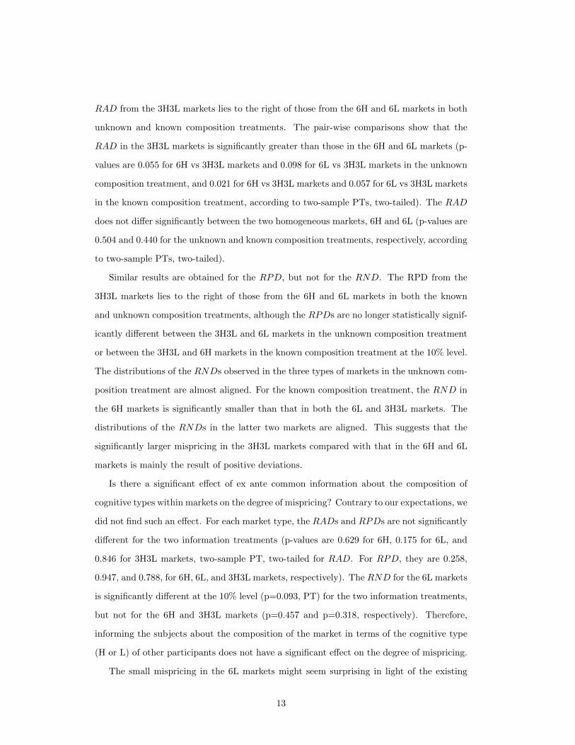
The top two panels in Figure 4 show the observed dynamics of trading volume from the
unknown (top) and known (middle) composition treatments. The three types of markets,
6H (left), 3H3L (center), and 6L (right), are shown separately for each treatment. While
the trading volumes seem to be higher in the 3H3L markets than in the 6H and 6L markets
for the unknown composition treatment, the opposite seems to be the case for the known
composition treatment. We also note that in many markets, there are periods with zero
transactions.14
The bottom panel in Figure 4 shows the empirical cumulative distribution of turnover,∑p Q
mp /24, where Qm
p is the realized trade volume in period p of market m. It can be seen
that there is no statistically significant difference across the three types of markets in the
two information treatments, except for the 6H and 3H3L markets in the known composition
treatment. Furthermore, except for the 3H3L markets, there are no statistically significant
14Our price determination procedure returns a price even in the absence of transactions.
14
Dynamics of volume: Unknown composition6H (8 markets) 3H3L (8 markets) 6L (8 markets)
0 5 10 15 20t
5
10
15
20
Q
0 5 10 15 20t
5
10
15
20
Q
0 5 10 15 20t
5
10
15
20
Q
Dynamics of volume: Known composition6H (12 markets) 3H3L (12 markets) 6L (12 markets)
0 5 10 15 20t
5
10
15
20
Q
0 5 10 15 20t
5
10
15
20
Q
0 5 10 15 20t
5
10
15
20
Q
Turnover: unknown composition Turnover: known composition
0.0 0.5 1.0 1.5 2.0 2.5 3.0TO0.0
0.2
0.4
0.6
0.8
1.0CDF
0.0 0.5 1.0 1.5 2.0 2.5 3.0TO0.0
0.2
0.4
0.6
0.8
1.0CDF
6L 3H3L6H 0.994 0.3696L 0.464
6L 3H3L6H 0.779 0.0886L 0.152
Figure 4: Top: realized trade volume dynamics in unknown (top) and known (bottom)composition treatments. Three types of markets are shown: 6H (left), 3H3L (center), and6L (right). Bottom: empirical cumulative distribution of turnover in unknown (left) andknown (right) composition treatments. In each panel, three market types are shown: 6H(thick, solid red line), 6L (thick, dashed blue line), and 3H3L (thin black line). The tablebelow each panel reports the p-values from pair-wise comparisons based on two-sample PTs,two-sided.
15
Unknown composition Known composition
0.0 0.2 0.4 0.6 0.8 1.0 1.2 1.4vRAD0.0
0.2
0.4
0.6
0.8
1.0CDF
0.0 0.2 0.4 0.6 0.8 1.0 1.2 1.4vRAD0.0
0.2
0.4
0.6
0.8
1.0CDF
6L 3H3L6H 0.871 0.1476L 0.109
6L 3H3L6H 0.357 0.0806L 0.290
Figure 5: Distribution of vRAD in unknown (left) and known (right) composition treat-ments. In each panel, three market types are shown: 6H (thick, solid red line), 6L (thick,dashed blue line), and 3H3L (thin black line). The table below each panel reports thep-values from pair-wise comparisons based on two-sample PTs, two-sided.
differences in turnover between the two information treatments (p-values are 0.367, 0.592,
and 0.095 for the 6H, 6L, and 3H3L markets, respectively).
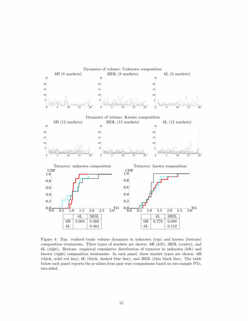
It is possible that the significantly larger mispricing we observed in the heterogeneous
markets (3H3L) compared with the homogeneous markets (6H and 6L) is the result of
mispricing that only occurred when the trading volume was zero or very low. If this is the
case, the straight measure of mispricing, RAD, that we have considered above overrepresents
the degree of mispricing. To address this potential problem, we define the volume-adjusted
RAD for market m, vRADm, as follows:
vRADm =1
20
20∑p=1
Qmp
( |Pmp − FVp||FV |
). (4)
Figure 5 shows the empirical cumulative distributions of vRAD in unknown (left) and
known (right) composition treatments. In each panel, three market types are shown: 6H
(thick, solid red line), 6L (thick, dashed blue line), and 3H3L (thin black line). However,
these distributions are ordered in a similar manner to those of RAD shown in Figure 3
above. For the unknown composition treatment, the distributions of vRAD for the two
homogeneous markets are almost aligned, while that for the 3H3L markets lies to the right
of them. For the known composition treatment, the distribution of vRAD for the 6H markets
lies to the left of that for the 6L markets, which in turn lies to the left of that for the 3H3L
16
markets. As in the case with RAD, there is no statistically significant difference in vRAD
between the two information treatments in each market type (p-values are 0.833 for 6H,
0.116 for 6L, and 0.728 for 3H3L markets based on two-sample PTs, two-tailed).
However, unlike the case of RADs, vRADs are no longer statistically significantly dif-
ferent between the heterogeneous markets and the homogeneous markets, except between
3H3L and 6H markets with known composition (p-values are 0.080 for 6H vs 3H3L markets,
0.290 for 6L vs 3H3L markets, and 0.357 for 6H vs 6L markets for the known composition
treatment, and 0.147 for 6H vs 3H3L markets, 0.109 for 6L vs 3H3L markets, and 0.871
for 6H vs 6L markets for the unknown composition treatment based on two-sample PTs,
two-tailed). This suggests that the mispricing in periods with zero or a low number of
transactions does indeed explain a part of the larger mispricing in the heterogeneous market
compared with the homogeneous market, but that is not the whole story.
Note, however, that if we pool the known and unknown composition treatments (because
there is no statistically significant difference between the two treatments in any of the three
types of markets), the vRADs for the 3H3L markets are significantly greater than those for
the 6H and 6L markets (p-values are 0.014 for 6H vs 3H3L markets, 0.043 for 6L vs 3H3L
markets, and 0.445 for 6H vs 6L markets).
3.3 Gender composition
In our analyses above, we have not controlled for the possible effects of gender composition
on mispricing. Eckel and Fullbrunn (2015) found that experimental asset markets with a
larger proportion of female subjects experienced smaller mispricing. Cueva and Rustichini
(2015) compared all-female, all-male, and mixed-gender markets and found that the mixed-
gender markets resulted in smaller mispricing than the other two types of markets. In this
subsection, we report the results of linear regression analyses investigating the relationship
between the cognitive ability of market participants and the degree of mispricing while
controlling for gender composition. Because we found no significant differences between
known and unknown composition treatments, we pooled the data from these two treatments
for the following analyses.
The dependent variables are the four mispricing measures we considered above: RAD,
RPD, RND, and vRAD. The independent variables are the mean and standard deviation
17
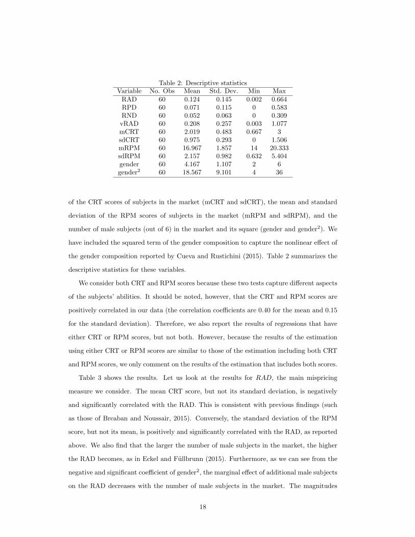
Table 2: Descriptive statisticsVariable No. Obs Mean Std. Dev. Min Max
RAD 60 0.124 0.145 0.002 0.664RPD 60 0.071 0.115 0 0.583RND 60 0.052 0.063 0 0.309vRAD 60 0.208 0.257 0.003 1.077mCRT 60 2.019 0.483 0.667 3sdCRT 60 0.975 0.293 0 1.506mRPM 60 16.967 1.857 14 20.333sdRPM 60 2.157 0.982 0.632 5.404gender 60 4.167 1.107 2 6gender2 60 18.567 9.101 4 36
of the CRT scores of subjects in the market (mCRT and sdCRT), the mean and standard
deviation of the RPM scores of subjects in the market (mRPM and sdRPM), and the
number of male subjects (out of 6) in the market and its square (gender and gender2). We
have included the squared term of the gender composition to capture the nonlinear effect of
the gender composition reported by Cueva and Rustichini (2015). Table 2 summarizes the
descriptive statistics for these variables.
We consider both CRT and RPM scores because these two tests capture different aspects
of the subjects’ abilities. It should be noted, however, that the CRT and RPM scores are
positively correlated in our data (the correlation coefficients are 0.40 for the mean and 0.15
for the standard deviation). Therefore, we also report the results of regressions that have
either CRT or RPM scores, but not both. However, because the results of the estimation
using either CRT or RPM scores are similar to those of the estimation including both CRT
and RPM scores, we only comment on the results of the estimation that includes both scores.
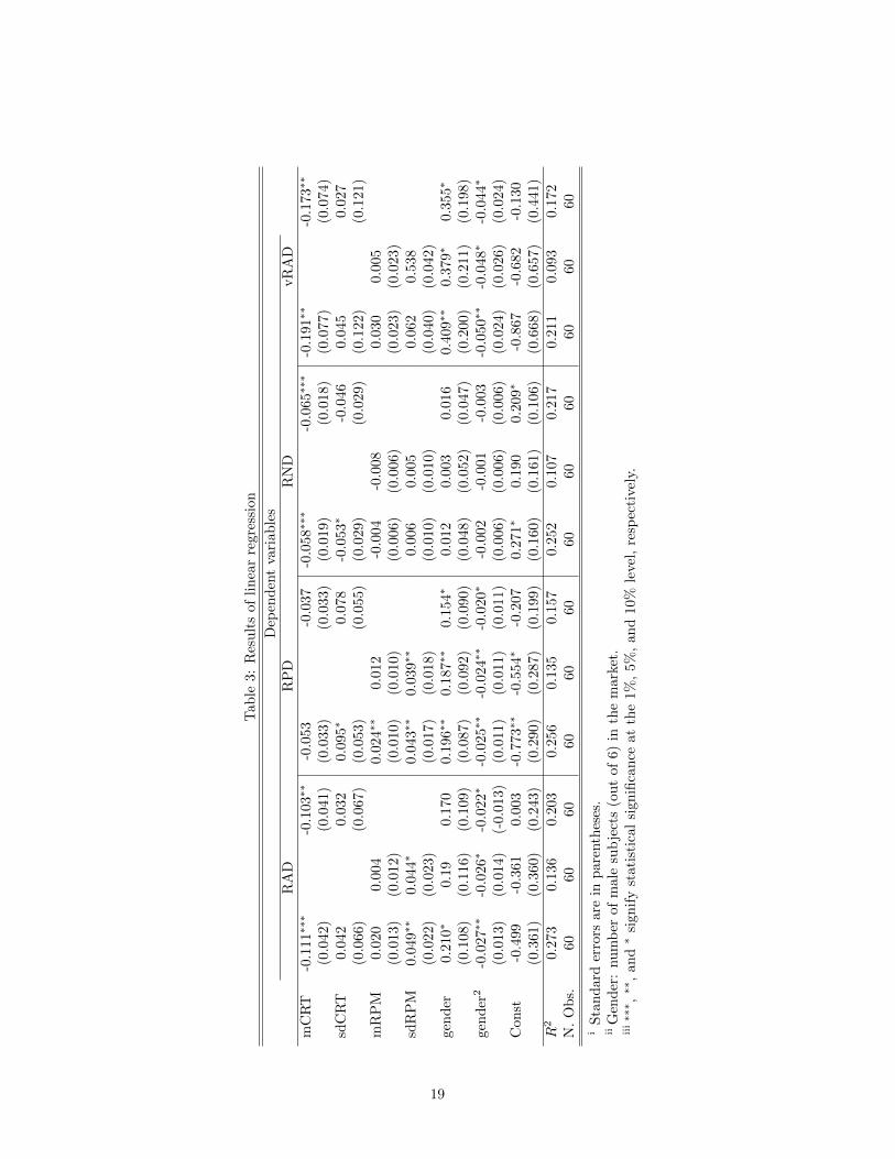
Table 3 shows the results. Let us look at the results for RAD, the main mispricing
measure we consider. The mean CRT score, but not its standard deviation, is negatively
and significantly correlated with the RAD. This is consistent with previous findings (such
as those of Breaban and Noussair, 2015). Conversely, the standard deviation of the RPM
score, but not its mean, is positively and significantly correlated with the RAD, as reported
above. We also find that the larger the number of male subjects in the market, the higher
the RAD becomes, as in Eckel and Fullbrunn (2015). Furthermore, as we can see from the
negative and significant coefficient of gender2, the marginal effect of additional male subjects
on the RAD decreases with the number of male subjects in the market. The magnitudes
18
Tab
le3:
Res
ult
sof
lin
ear
regre
ssio
n
Dep
end
ent
vari
ab
les
RA
DR
PD
RN
DvR
AD
mC
RT
-0.1
11∗∗∗
-0.1
03∗∗
-0.0
53
-0.0
37
-0.0
58∗∗∗
-0.0
65∗∗∗
-0.1
91∗∗
-0.1
73∗∗
(0.0
42)
(0.0
41)
(0.0
33)
(0.0
33)
(0.0
19)
(0.0
18)
(0.0
77)
(0.0
74)
sdC
RT
0.04
20.
032
0.095∗
0.0
78
-0.0
53∗
-0.0
46
0.0
45
0.0
27
(0.0
66)
(0.0
67)
(0.0
53)
(0.0
55)
(0.0
29)
(0.0
29)
(0.1
22)
(0.1
21)
mR
PM
0.02
00.
004
0.02
4∗∗
0.0
12
-0.0
04
-0.0
08
0.0
30
0.0
05
(0.0
13)
(0.0
12)
(0.0
10)
(0.0
10)
(0.0
06)
(0.0
06)
(0.0
23)
(0.0
23)
sdR
PM
0.04
9∗∗
0.04
4∗
0.04
3∗∗
0.0
39∗∗
0.0
06
0.0
05
0.0
62
0.5
38
(0.0
22)
(0.0
23)
(0.0
17)
(0.0
18)
(0.0
10)
(0.0
10)
(0.0
40)
(0.0
42)
gen
der
0.21
0∗
0.19
0.17
00.
196∗∗
0.1
87∗∗
0.1
54∗
0.0
12
0.0
03
0.0
16
0.4
09∗∗
0.3
79∗
0.3
55∗
(0.1
08)
(0.1
16)
(0.1
09)
(0.0
87)
(0.0
92)
(0.0
90)
(0.0
48)
(0.0
52)
(0.0
47)
(0.2
00)
(0.2
11)
(0.1
98)
gen
der
2-0
.027∗∗
-0.0
26∗
-0.0
22∗
-0.0
25∗∗
-0.0
24∗∗
-0.0
20∗
-0.0
02
-0.0
01
-0.0
03
-0.0
50∗∗
-0.0
48∗
-0.0
44∗
(0.0
13)
(0.0
14)
(-0.
013)
(0.0
11)
(0.0
11)
(0.0
11)
(0.0
06)
(0.0
06)
(0.0
06)
(0.0
24)
(0.0
26)
(0.0
24)
Con
st-0
.499
-0.3
610.
003
-0.7
73∗∗
-0.5
54∗
-0.2
07
0.2
71∗
0.1
90
0.2
09∗
-0.8
67
-0.6
82
-0.1
30
(0.3
61)
(0.3
60)
(0.2
43)
(0.2
90)
(0.2
87)
(0.1
99)
(0.1
60)
(0.1
61)
(0.1
06)
(0.6
68)
(0.6
57)
(0.4
41)
R2
0.27
30.
136
0.20
30.
256
0.1
35
0.1
57
0.2
52
0.1
07
0.2
17
0.2
11
0.0
93
0.1
72
N.
Ob
s.60
6060
6060
60
60
60
60
60
60
60
iS
tan
dar
der
rors
are
inp
aren
thes
es.
iiG
end
er:
nu
mb
erof
mal
esu
bje
cts
(out
of6)
inth
em
ark
et.
iii∗∗∗ ,∗∗
,an
d∗
sign
ify
stat
isti
cal
sign
ifica
nce
at
the
1%
,5%
,an
d10%
leve
l,re
spec
tivel
y.
19

of the estimated coefficient of gender and its squared term show that there is an inverse-U-
shaped relationship between the number of male subjects in the market and the extent of
mispricing, as in Cueva and Rustichini (2015).
The results are similar for the RPD, the differences from the results in relation to the
RAD being that the mean CRT score loses its statistical significance, while the mean RPM
scores and the standard deviation of CRT scores become statistically significant. The stan-
dard deviation of RPM scores remains positively significantly correlated with the RPD.15
Thus, even after controlling for the potential effects of gender composition, the heterogene-
ity in cognitive ability among market participants increases the mispricing, especially the
positive deviation in prices from FV.
The results are quite different for the RND. For the RND, either the mean or the
standard deviation of the RPM scores is statistically significant. Further, the gender com-
position (both the term and its square) is not statistically significant. However, the mean
CRT score is significantly negative in this regression.
Finally, for the (vRAD), while the mean CRT score remains statistically significantly
negative, both the mean and standard deviation of the RPM scores become statistically
insignificant once the gender composition is controlled for. The gender composition effect
remains statistically significant, with the same sign as in the case of the RAD.
3.4 Heterogeneity in trading behavior and mispricing
Why does heterogeneity in cognitive ability increase mispricing? We hypothesize that het-
erogeneity in cognitive ability results in heterogeneity in trading behavior, which results in
larger price variations and mispricing.
To capture the heterogeneity in trading behavior among market participants, we compute
the standard deviation of bids and asks submitted by market participants for each period
in each market, and take the average across 20 periods. Figure 6 shows the empirical
cumulative distributions of the within-market standard deviations of bids (left) and asks
(right). It can be seen from the left panel that within-market bid heterogeneity is largest in
the 3H3L markets and smallest in the 6H markets. As the table below the left panel shows,
15It is also interesting to note the significant positive coefficient of mRPM. However, we do not have avery clear interpretation of this result.
20
s.d. Bids s.d. Asks
0 20 40 60 80 100sdBid
0.2
0.4
0.6
0.8
1.0CDF
0 20 40 60 80 100sdAsk0.0
0.2
0.4
0.6
0.8
1.0CDF
6L 3H3L6H 0.020 < 0.0016L 0.078
6L 3H3L6H 0.863 0.8756L 0.976
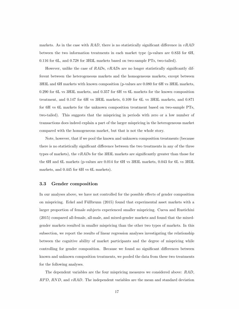
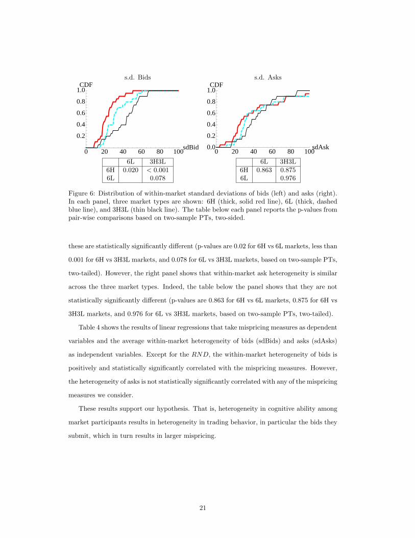
Figure 6: Distribution of within-market standard deviations of bids (left) and asks (right).In each panel, three market types are shown: 6H (thick, solid red line), 6L (thick, dashedblue line), and 3H3L (thin black line). The table below each panel reports the p-values frompair-wise comparisons based on two-sample PTs, two-sided.
these are statistically significantly different (p-values are 0.02 for 6H vs 6L markets, less than
0.001 for 6H vs 3H3L markets, and 0.078 for 6L vs 3H3L markets, based on two-sample PTs,
two-tailed). However, the right panel shows that within-market ask heterogeneity is similar
across the three market types. Indeed, the table below the panel shows that they are not
statistically significantly different (p-values are 0.863 for 6H vs 6L markets, 0.875 for 6H vs
3H3L markets, and 0.976 for 6L vs 3H3L markets, based on two-sample PTs, two-tailed).
Table 4 shows the results of linear regressions that take mispricing measures as dependent
variables and the average within-market heterogeneity of bids (sdBids) and asks (sdAsks)
as independent variables. Except for the RND, the within-market heterogeneity of bids is
positively and statistically significantly correlated with the mispricing measures. However,
the heterogeneity of asks is not statistically significantly correlated with any of the mispricing
measures we consider.
These results support our hypothesis. That is, heterogeneity in cognitive ability among
market participants results in heterogeneity in trading behavior, in particular the bids they
submit, which in turn results in larger mispricing.
21
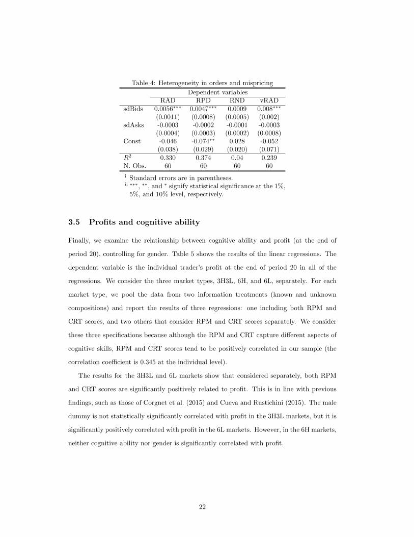
Table 4: Heterogeneity in orders and mispricing
Dependent variablesRAD RPD RND vRAD
sdBids 0.0056∗∗∗ 0.0047∗∗∗ 0.0009 0.008∗∗∗
(0.0011) (0.0008) (0.0005) (0.002)sdAsks -0.0003 -0.0002 -0.0001 -0.0003
(0.0004) (0.0003) (0.0002) (0.0008)Const -0.046 -0.074∗∗ 0.028 -0.052
(0.038) (0.029) (0.020) (0.071)R2 0.330 0.374 0.04 0.239N. Obs. 60 60 60 60
i Standard errors are in parentheses.ii ∗∗∗, ∗∗, and ∗ signify statistical significance at the 1%,
5%, and 10% level, respectively.
3.5 Profits and cognitive ability
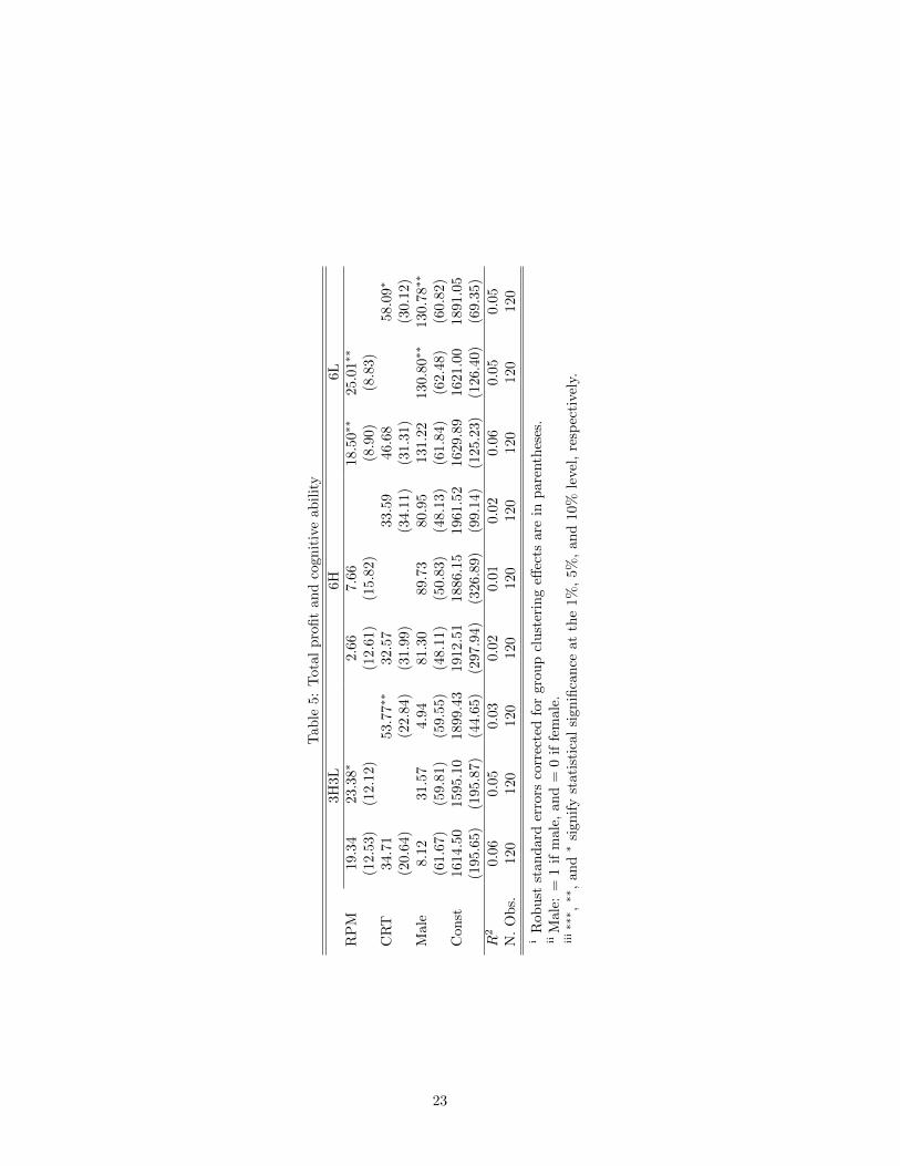
Finally, we examine the relationship between cognitive ability and profit (at the end of
period 20), controlling for gender. Table 5 shows the results of the linear regressions. The
dependent variable is the individual trader’s profit at the end of period 20 in all of the
regressions. We consider the three market types, 3H3L, 6H, and 6L, separately. For each
market type, we pool the data from two information treatments (known and unknown
compositions) and report the results of three regressions: one including both RPM and
CRT scores, and two others that consider RPM and CRT scores separately. We consider
these three specifications because although the RPM and CRT capture different aspects of
cognitive skills, RPM and CRT scores tend to be positively correlated in our sample (the
correlation coefficient is 0.345 at the individual level).
The results for the 3H3L and 6L markets show that considered separately, both RPM
and CRT scores are significantly positively related to profit. This is in line with previous
findings, such as those of Corgnet et al. (2015) and Cueva and Rustichini (2015). The male
dummy is not statistically significantly correlated with profit in the 3H3L markets, but it is
significantly positively correlated with profit in the 6L markets. However, in the 6H markets,
neither cognitive ability nor gender is significantly correlated with profit.
22
Tab
le5:
Tota
lp
rofi
tan
dco
gn
itiv
eab
ilit
y
3H3L
6H
6L
RP
M19
.34
23.3
8∗
2.6
67.6
618.5
0∗∗
25.0
1∗∗
(12.
53)
(12.
12)
(12.6
1)
(15.8
2)
(8.9
0)
(8.8
3)
CR
T34
.71
53.7
7∗∗
32.5
733.5
946.6
858.0
9∗
(20.
64)
(22.8
4)
(31.9
9)
(34.1
1)
(31.3
1)
(30.1
2)
Mal
e8.
1231
.57
4.9
481.3
089.7
380.9
5131.2
2130.8
0∗∗
130.7
8∗∗
(61.
67)
(59.
81)
(59.5
5)
(48.1
1)
(50.8
3)
(48.1
3)
(61.8
4)
(62.4
8)
(60.8
2)
Con
st161
4.50
1595
.10
1899.4
31912.5
11886.1
51961.5
21629.8
91621.0
01891.0
5(1
95.6
5)(1
95.8
7)(4
4.6
5)
(297.9
4)
(326.8
9)
(99.1
4)
(125.2
3)
(126.4
0)
(69.3
5)
R2
0.06
0.05
0.0
30.0
20.0
10.0
20.0
60.0
50.0
5N
.O
bs.
120
120
120
120
120
120
120
120
120
iR
obu
stst
and
ard
erro
rsco
rrec
ted
for
gro
up
clu
ster
ing
effec
tsare
inp
are
nth
eses
.ii
Mal
e:=
1if
mal
e,an
d=
0if
fem
ale
.iii∗∗∗ ,∗∗
,an
d∗
sign
ify
stat
isti
cal
sign
ifica
nce
at
the
1%
,5%
,an
d10%
leve
l,re
spec
tivel
y.
23
4 Summary and conclusion
How does the average cognitive ability among market participants, as well as their diversity,
influence mispricing in an experimental market? We investigated this question by first
measuring an aspect of the cognitive ability of our subjects using the RPM test, and then
constructing markets by grouping subjects based on their relative test scores. We defined
those subjects whose scores were above and below the median score as H type and L type,
respectively. We then considered three kinds of markets: those in which all six traders were
H type (6H), those in which all six traders were L type (6L), and those in which H and L
types were equally mixed (3H3L).
To investigate whether knowledge of the heterogeneity of cognitive ability among market
participants can have an additional effect on mispricing, we considered two information
treatments: the known composition treatment and the unknown composition treatment.
In both treatments, we informed our subjects of their own type (H or L). In the known
composition treatment, we also informed them of the types of the other five traders in their
market. Thus, for example, those in the 6H markets were informed that they were H type
and the other five traders in the same market were also H type. In the unknown composition
treatment, this information was not provided.
Contrary to what one may infer from the results of earlier experimental studies that
found a negative relationship between the average cognitive ability of subjects in a market
and the degree of mispricing, the degree of mispricing observed in the 3H3L markets was
significantly larger than that observed in the 6H and 6L markets in both the known and
unknown composition treatments. Thus, it is not only the average cognitive ability of traders
in the market but also the diversity in cognitive ability that matters when it comes to the
degree of mispricing. However, contrary to our expectations, we did not find any significant
additional effect of heterogeneity being ex ante known on the degree of mispricing.
We hypothesized that the reason for the larger mispricing in the 3H3L markets compared
with that in the 6H and 6L markets was the positive correlation between heterogeneity in
cognitive ability among market participants and heterogeneity in their trading behavior,
and that this heterogeneity in trading behavior generated larger mispricing. Our analysis
supports this hypothesis. The within-market heterogeneity of submitted bids was signifi-
24
cantly larger in the 3H3L markets than in the 6H or 6L markets, and this heterogeneity
was significantly positively correlated with mispricing measures. We believe that a more
in-depth analysis of heterogeneity in trading behavior dynamics can be a fruitful area for
future research. However, it may be useful to conduct experiments for this purpose under
continuous double auction conditions to enable more observations to be gathered about the
dynamics of trading behavior.
Recently, several researchers have investigated the effects of other types of heterogeneity
on mispricing in a similar experimental setup. Levine et al. (2014) report that knowledge
of ethnic diversity among market participants reduces the degree of mispricing. Their in-
terpretation of the data is that participants do not think critically about others’ decisions
in ethnically homogeneous markets, and thus tend to ride “bubbles” compared with partic-
ipants in ethnically diverse markets.
Eckel and Fullbrunn (2015) and Cueva and Rustichini (2015) study the effect of gen-
der composition on mispricing and disagree somewhat in their findings. While Eckel and
Fullbrunn (2015) find that all-male markets generate higher levels of mispricing than all-
female markets and the mispricing observed in mixed-gender markets falls between the two,
Cueva and Rustichini (2015) find that mispricing in mixed-gender markets is larger than
that in both all-male and all-female markets. Our regression result is in line with that of
Cueva and Rustichini (2015), in that while an increasing proportion of male participants
in a market increases the degree of mispricing, its marginal effect is negative, which results
in an inverted-U-shaped relationship between the proportion of male participants in the
market and the degree of mispricing.
Hefti et al. (2016) consider the effect of heterogeneity in relation to two distinct capa-
bilities: analytical capability (cognitive skills) and mentalizing capability (the theory of the
mind). They find that, consistent with their hypotheses, to be successful in asset-market
experiments, one has to have both high analytical capabilities and high mentalizing capabil-
ities because one’s success depends on understanding not only market fundamentals (which
requires analytical capability) but also the price dynamics resulting from the behavior of
other participants (which requires mentalizing capability). It will be very interesting to
undertake future research constructing various types of markets by grouping subjects based
on heterogeneity in various dimensions such as gender, ethnic identity, analytical capability,
25
and mentalizing capability to investigate how heterogeneities in these various dimensions
interact among themselves and determine aggregate market outcomes.
References
Aggarwal, R. K. and G. Wu (2006): “Stock Market Manipulations,” Journal of Busi-
ness, 79, 1915–1953.
Akiyama, E., N. Hanaki, and R. Ishikawa (2014): “How do experienced traders respond
to inflows of inexperienced traders? An experimental analysis,” Journal of Economic
Dynamics and Control, 45, 1–18.
——— (2015): “It is not just confusion! Strategic uncertainty in an experimental asset
market,” Economic Journal, forthcoming.
Allen, F. and D. Gale (1992): “Stock-Price Manipulation,” Review of Financial Studies,
5, 503–529.
Allen, F., S. Morris, and H. S. Shin (2006): “Beauty Contests and Iterated Expecta-
tions in Asset Markets,” The Review of Financial Studies, 19, 719–752.
Bosch-Rosa, C., T. Meissner, and A. Bosch-Domenech (2015): “Cognitive Bubbles,”
Mimeo, Berlin University of Technology.
Breaban, A. and C. N. Noussair (2015): “Trader characteristics and fundamental value
trajectories in an asset market experiment,” Journal of Behavioral and Experimental
Finance, 8, 1–17.
Carpenter, J., M. Graham, and J. Wolf (2013): “Cognitive ability and strategic
sophistication,” Games and Economic Behavior, 80, 115–130.
Cheung, S. L., M. Hedegaard, and S. Palan (2014): “To See is To Believe: Common
Expectations in Experimental Asset Markets,” European Economic Review, 66, 84–96.
Corgnet, B., R. H. Gonzalez, P. Kujal, and D. Porter (2015): “The Effect of
Earned vs. House Money on Price Bubble Formation in Experimental Asset Markets,”
Review of Finance, 19, 1455–1488.
26
Cueva, C. and A. Rustichini (2015): “Is financial instability male-driven? Gender
and cognitive skills in experimental asset markets,” Journal of Economic Behavior and
Organization, 119, 330–344.
Dohmen, T., A. Falk, D. Huffman, and U. Sunde (2010): “Are risk aversion and
impatience related to cognitive ability?” American Economic Review, 100, 1238–1260.
Dufwenberg, M., R. Sundaram, and D. J. Butler (2010): “Epiphany in the Game
of 21,” Journal of Economic Behavior and Organization, 75, 132–143.
Eckel, C. C. and S. C. Fullbrunn (2015): “Thar SHE Blows? Gender, competition,
and bubbles in experimental asset markets,” American Economic Review, 105, 906–920.
Fischbacher, U. (2007): “z-Tree: Zurich toolbox for ready-made economic experiments,”
Experimental Economics, 10, 171–178.
Frederick, S. (2005): “Cognitive reflection and decision making,” Journal of Economic
Perspectives, 19, 25–42.
Gill, D. and V. Prowse (2016): “Cognitive ability, character skills, and learning to play
equilibrium: A level-k analysis,” Journal of Political Economy, 124, 1619–1676.
Gneezy, U., A. Rustichini, and A. Vostroknutov (2010): “Experience and insight
in the Race game,” Journal of Economic Behavior and Organization, 144–155.
Haruvy, E., Y. Lahav, and C. N. Noussair (2007): “Traders’ Expectations in Asset
Markets: Experimental Evidence,” American Economics Review, 97, 1901–1920.
Hefti, A., S. Heinke, and F. Schneider (2016): “Mental Capabilities, Trading Styles,
and Asset Market Bubbles: Theory and Experiment,” Working Paper Series 234, Depart-
ment of Economics, University of Zurich.
Kindleberger, C. P. and R. Z. Aliber (2005): Manias, Panics, and Crashes. A History
of Financial Crises. 5th Edition, Hoboken, New Jersey: John Wiley & Sons, Inc.
Korniotis, G. M. and A. Kumar (2010): “Cognitive abilities and financial decisions,” in
Behavioral Finance: Investors, Corporations, and Markets, ed. by H. K. Baker and J. R.
Nofsinger, Hoboken, New Jersey: John Wiley & Sons, Inc., chap. 30, 559–576.
27
Levine, S. S., E. P. Apfelbaum, M. Bernard, V. L. Bartelt, E. J. Zajac, and
D. Stark (2014): “Ethinic diversity deflates price bubbles,” Proceedings of the National
Academies of Sciences, 111, 18524–18529.
Lopez, L. (2015): “6can’t read,” Business Insider.
Mullainathan, S. and E. Shafir (2013): Scarcity: Why Having Too Little Means So
Much, New York, NY: Times Books, Henry Holt and Company, LLC.
Oechssler, J., A. Roider, and P. W. Schmitz (2009): “Cognitive abilities and behav-
ioral biases,” Journal of Economic Behavior and Organization, 72, 147–152.
Palan, S. (2013): “A Review of bubbles and crashes in experimental asset markets,”
Journal of Economic Surveys, 27, 570–588.
Porter, D. P. and V. L. Smith (1995): “Futures contracting and dividend uncertainty
in experimental asset markets,” The Journal of Business, 68, 509–541.
Powell, O. and N. Shestakova (2016): “Experimental asset markets: A survey of recent
developments,” Journal of Behavioral and Experimental Finance, 12, 14–22.
Proto, E., A. Rustichini, and A. Sofianos (2016): “Intelligence, personality and gains
from cooperation in repeated interactions,” Workinng paper, University of Warwick.
Raven, J. (2008): “General introduction and overview: the raven progressive matrices
tests: their theoretical basis and measurement model,” in Uses and abuses of intelligence,
ed. by John and J. Raven, Edinburgh, Scotland: Competency Motivation Project, chap. 1,
17–68.
Smith, V. L., G. L. Suchanek, and A. W. Williams (1988): “Bubbles, Crashes, and
Endogenous Expectations in Experimental Spot Asset Markets,” Econometrica, 56, 1119–
1151.
Stockl, T., J. Huber, and M. Kirchler (2010): “Bubble measures in Experimental
Asset Markets,” Experimental Economics, 13, 284–298.
van Boening, M. V., A. W. Williams, and S. LaMaster (1993): “Price bubbles and
crashes in experimental call markets,” Economics Letters, 41, 179–185.
28

Xiong, W. and J. Yu (2011): “The Chinese warrants bubble,” American Economic Re-
view, 101, 2723–2753.
29
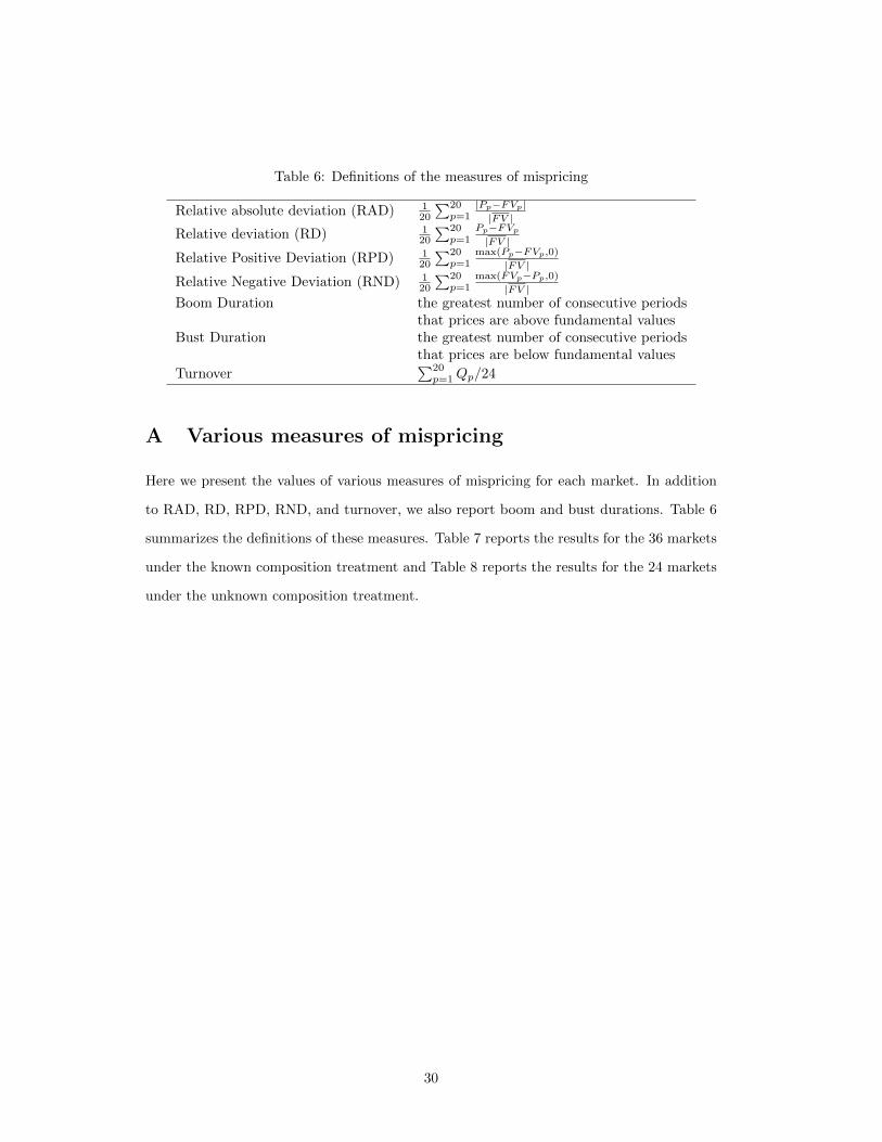
Table 6: Definitions of the measures of mispricing
Relative absolute deviation (RAD) 120
∑20p=1
|Pp−FVp||FV |
Relative deviation (RD) 120
∑20p=1
Pp−FVp
|FV |
Relative Positive Deviation (RPD) 120
∑20p=1
max(Pp−FVp,0)
|FV |
Relative Negative Deviation (RND) 120
∑20p=1
max(FVp−Pp,0)
|FV |Boom Duration the greatest number of consecutive periods
that prices are above fundamental valuesBust Duration the greatest number of consecutive periods
that prices are below fundamental values
Turnover∑20
p=1 Qp/24
A Various measures of mispricing
Here we present the values of various measures of mispricing for each market. In addition
to RAD, RD, RPD, RND, and turnover, we also report boom and bust durations. Table 6
summarizes the definitions of these measures. Table 7 reports the results for the 36 markets
under the known composition treatment and Table 8 reports the results for the 24 markets
under the unknown composition treatment.
30
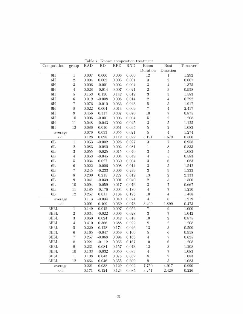
Table 7: Known composition treatmentComposition group RAD RD RPD RND Boom Bust Turnover
Duration Duration6H 1 0.007 0.006 0.006 0.000 12 1 1.2926H 2 0.004 0.002 0.003 0.001 3 2 0.6676H 3 0.006 -0.001 0.002 0.004 3 4 1.3756H 4 0.028 -0.014 0.007 0.021 2 3 0.9586H 5 0.153 0.130 0.142 0.012 3 3 1.5836H 6 0.019 -0.008 0.006 0.014 2 4 0.7926H 7 0.076 -0.010 0.033 0.043 5 5 1.9176H 8 0.022 0.004 0.013 0.009 7 4 2.4176H 9 0.456 0.317 0.387 0.070 10 7 0.8756H 10 0.006 -0.001 0.003 0.004 5 2 1.2086H 11 0.048 -0.043 0.002 0.045 3 5 1.1256H 12 0.086 0.016 0.051 0.035 5 2 1.083
average 0.076 0.033 0.055 0.021 5 4 1.274s.d. 0.128 0.098 0.112 0.022 3.191 1.679 0.500
6L 1 0.053 -0.002 0.026 0.027 3 7 0.9586L 2 0.083 -0.080 0.002 0.081 1 8 0.8336L 3 0.055 -0.025 0.015 0.040 3 5 1.0836L 4 0.053 -0.045 0.004 0.049 4 5 0.5836L 5 0.034 0.027 0.030 0.004 3 6 1.0836L 6 0.022 -0.006 0.008 0.014 3 5 1.5426L 7 0.245 -0.233 0.006 0.239 3 9 1.3336L 8 0.239 0.215 0.227 0.012 13 2 2.3336L 9 0.041 -0.039 0.001 0.040 2 5 1.5006L 10 0.094 -0.059 0.017 0.076 3 7 0.6676L 11 0.185 -0.176 0.004 0.180 4 7 1.2506L 12 0.257 0.011 0.134 0.123 10 4 1.458
average 0.113 -0.034 0.040 0.074 4 6 1.219s.d. 0.091 0.109 0.069 0.073 3.499 1.899 0.473
3H3L 1 0.149 0.045 0.097 0.052 7 9 1.0003H3L 2 0.034 -0.022 0.006 0.028 3 7 1.0423H3L 3 0.060 0.024 0.042 0.018 10 2 0.8753H3L 4 0.410 0.366 0.388 0.022 8 2 1.2083H3L 5 0.220 0.128 0.174 0.046 13 3 0.5003H3L 6 0.165 -0.047 0.059 0.106 5 6 0.9583H3L 7 0.257 -0.068 0.094 0.163 4 7 0.6253H3L 8 0.221 -0.112 0.055 0.167 10 6 1.2083H3L 9 0.231 0.084 0.157 0.073 12 3 1.2083H3L 10 0.133 -0.032 0.050 0.083 4 7 1.0833H3L 11 0.108 0.043 0.075 0.032 8 2 1.0833H3L 12 0.664 0.046 0.355 0.309 9 5 1.083
average 0.221 0.038 0.129 0.092 7.750 4.917 0.990s.d. 0.171 0.124 0.123 0.085 3.251 2.429 0.226
31
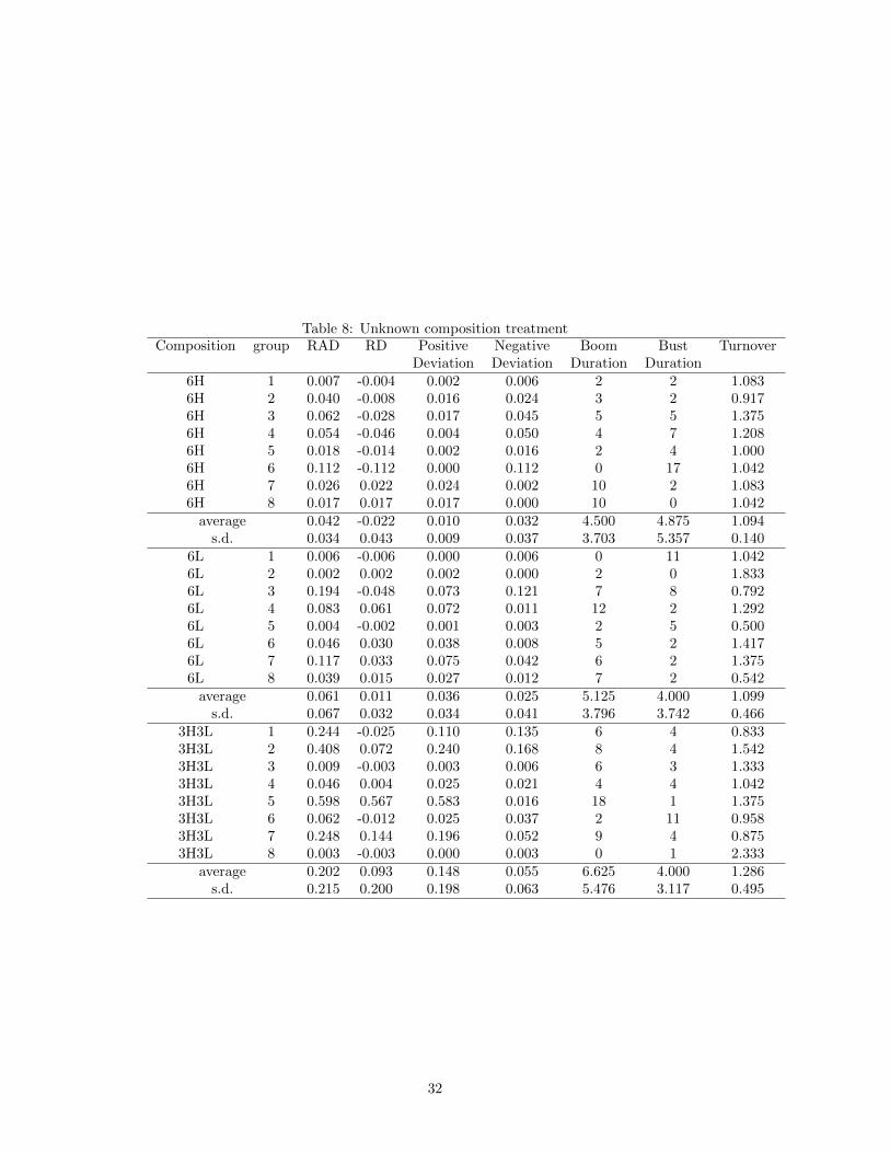
Table 8: Unknown composition treatmentComposition group RAD RD Positive Negative Boom Bust Turnover
Deviation Deviation Duration Duration6H 1 0.007 -0.004 0.002 0.006 2 2 1.0836H 2 0.040 -0.008 0.016 0.024 3 2 0.9176H 3 0.062 -0.028 0.017 0.045 5 5 1.3756H 4 0.054 -0.046 0.004 0.050 4 7 1.2086H 5 0.018 -0.014 0.002 0.016 2 4 1.0006H 6 0.112 -0.112 0.000 0.112 0 17 1.0426H 7 0.026 0.022 0.024 0.002 10 2 1.0836H 8 0.017 0.017 0.017 0.000 10 0 1.042
average 0.042 -0.022 0.010 0.032 4.500 4.875 1.094s.d. 0.034 0.043 0.009 0.037 3.703 5.357 0.140
6L 1 0.006 -0.006 0.000 0.006 0 11 1.0426L 2 0.002 0.002 0.002 0.000 2 0 1.8336L 3 0.194 -0.048 0.073 0.121 7 8 0.7926L 4 0.083 0.061 0.072 0.011 12 2 1.2926L 5 0.004 -0.002 0.001 0.003 2 5 0.5006L 6 0.046 0.030 0.038 0.008 5 2 1.4176L 7 0.117 0.033 0.075 0.042 6 2 1.3756L 8 0.039 0.015 0.027 0.012 7 2 0.542
average 0.061 0.011 0.036 0.025 5.125 4.000 1.099s.d. 0.067 0.032 0.034 0.041 3.796 3.742 0.466
3H3L 1 0.244 -0.025 0.110 0.135 6 4 0.8333H3L 2 0.408 0.072 0.240 0.168 8 4 1.5423H3L 3 0.009 -0.003 0.003 0.006 6 3 1.3333H3L 4 0.046 0.004 0.025 0.021 4 4 1.0423H3L 5 0.598 0.567 0.583 0.016 18 1 1.3753H3L 6 0.062 -0.012 0.025 0.037 2 11 0.9583H3L 7 0.248 0.144 0.196 0.052 9 4 0.8753H3L 8 0.003 -0.003 0.000 0.003 0 1 2.333
average 0.202 0.093 0.148 0.055 6.625 4.000 1.286s.d. 0.215 0.200 0.198 0.063 5.476 3.117 0.495
32

Appendix B
This Appendix contains English translation of the script used for the instruction videos. We have
distributed handouts based on the instruction videos that are shown to our subjects as well. The
handouts as well as the original instructions in Japanese are available from the authors upon request.
Please note that This is the common instruction of our experiments of 6H, 6L and 3H3L. For the
known-composition treatments, we announced the red-colored and blue-colored sentences
highlighted with [6H/6L] or [3H3L] for 6H/6L and 3H3L, respectively in addition to the
black-colored sentences. For the unknown-composition treatments, we announced only the
black-colored sentences.
Instructions for Today’s Experiment
Let’s start today’s experiment. We will explain it in the handout in front of you.
Please turn to the next page. First, you will be asked to take a quiz. After this quiz, the instructions for today’s game will be
explained to you. There will be a practice period for the game so that you may familiarize yourself
with the computer interface before the real experiment. Finally, we will ask you to respond to a
questionnaire and take quizzes. Your earnings will be paid in cash at the conclusion.
Your earnings will consist of a common participation fee of 500 yen, and the result of the game. The
questionnaire and quizzes will not impact your earnings. You will have a short bathroom break
before the game begins.
We will now explain the first quiz. This quiz consists of 24 questions to be answered within a 15
minute timeframe. For each question, you will view a set of pictures at the top of the screen that are
ordered according to a certain pattern. One picture is missing. Your task will be to guess the
underlying pattern, and then select the best suited replacement for the missing picture from among
the options shown at the bottom of the screen.
(The source of the picture used is Mullainathan and Shafir (2013, p.48). This sentence was not
shown to our subjects.)

Please turn to the next page. When the quiz begins, the following information will appear on the screen:
(1) This notes the time remaining. You have 900 seconds to answer as many of the 24 questions as
possible.
(2) This indicates the question number.
(3) This is the display of the question.
(4) This is where you will select your option from the corresponding choices found in the bottom
part of the picture in (3).
(5) You may request another question to an answer by entering that question number here. We will
explain this in detail in the following instructions.
Once you have determined the answer to a question, please select from the options shown on the
right side of the screen and click OK; the screen for the next question will appear. If you would like
to answer another question that is different from the one shown in the screen, please enter the
question number on the top left side of the screen and click GO. The screen for the question selected
will appear. You can return to the previous question by clicking the [Previous Q] button, or proceed
to the next question by clicking the [Next Q] button. If you would like to skip the present question,
please click the [Next Q] button without selecting any options. If you answer the same question
more than once, the computer will only record your last answer.
Please begin the quiz when the first question appears on the screen.

Instructions for the Stock Trading Experiment [Today’s experiment]
Today you will participate in a stock trading game in which you trade stocks in an artificial stock
market. Please listen to the instructions carefully and if you do not understand any part of an
instruction, ask for clarity by raising your hand. Moreover, if you have any questions during the
experiment, raise your hand and an instructor will come to you and answer your question.
Throughout the experiment, please respect the following rules:
1. Do not talk to the other participants during the experiment or the breaks.
ü This may affect the results of the experiment.
2. Use your mouse or keyboard only when instructed to do so by the instructor; otherwise, it may
cause a problem.
ü If any malfunction occurs, all participants will have to restart the game.
Please turn to the next page. [Outline of stock trading game]
You are divided into the top 12 scorers and the bottom 12 scorers of 24 people from the previous
quiz. Before starting the game, you will know which your rank is, the top or the bottom.
The 24 people in the room are divided into four groups, each of which consists of six people:
[6H/6L] Two of the four groups consist of the top scorers, and the other two groups consist of the
bottom scorers.
[3H3L] Each of four groups consists of three people in the top and three people in the bottom.
You play the stock trading game with other five people in the group you belong to.
[Objectives of the game]
Your objective in this game is to make as much profit as you can. We use Mark as the currency for
the experiment. At the end of the experiment, 1 Mark will be converted into 1 yen and paid out to
you. There are two ways of making a profit:
• First, you can realize a profit margin through buying and selling stocks.
• Second, you can earn dividends on your stock holdings.
Please turn to the next page. [Earning a profit margin]
You will be given four stocks + 1040 Marks at the beginning of the game. To earn a profit margin by
trading, you need to buy stocks at a lower price and sell these at a higher price. For example,
suppose you buy a stock for 100 Marks, and then the price of the stock increases to 120 Marks. If

you sell the stock, you will earn 120 (selling price) - 100 (purchase price) = 20 Marks profit. In
contrast, suppose you buy a stock for 100 Marks, and then the price of the stock decreases to 80
Marks. If you sell the stock, you will make 80 (selling price) - 100 (purchase price) = 20 Marks loss.
We will explain later how the prices are determined.
Now we will explain how to use the experimental program interface. We will also explain how to
earn a profit margin. Please do not perform any operations other than those which you are instructed
to carry out; otherwise, it may jeopardize our experiment.
Please double-click on the indicated icon on the computer screen.
[Order entry screen]
The following screen will appear, through which you can enter your orders for each time period.
(1) This shows the remaining time for entering your orders. The time limit to enter your order is 60
seconds. When the time has elapsed, a red warning message will flash at the top right corner of
your screen. A period ends once everyone has pressed “OK”; note that this could be within the
60 second time limit.
(2) This indicates your cash balance or the amount of money at your disposal; you may buy stocks
up to this amount.
(3) This shows the number of stocks you have. You may sell a maximum of this number of stocks.

(4) This is where you enter the maximum price you are willing to pay to buy a stock in this period.
You must enter a whole number between 1 and 2000.
(5) Here you need to enter the maximum number of stocks that you want to buy in this period. If
you do not want to purchase any stocks, enter 0. The product of (4) and (5) must be no greater
than your cash balance shown in (2). An error message will appear if (the number of stocks you
wish to buy) × (the maximum price you are prepared to pay for these) exceeds your cash
balance.
In practice, the price you actually pay for a stock may not be the same as the maximum price you are
willing to pay. This is because the market price is set based on all the orders placed by market
participants. If the market price is greater than the maximum you are willing to pay, your order will
not be processed. This will be further clarified at a later stage.
Please turn to the next page. (6) Here please enter the minimum price at which you would be prepared to sell your stocks in this
period. You must enter a whole number between 1 and 2000. The price you enter here should
not be greater than that given in (4).
(7) This is where you should enter the number of stocks you want to sell in this period. If you do
not want to sell any of your stocks, enter 0. The maximum number of stocks you can sell is the
number of stocks you hold, as shown in (3). If the number of stocks you want to sell exceeds
the number of stocks you hold, an error message will appear.
In practice, the price at which you sell a stock may not be the same as the minimum price at which
you are willing to sell. This is because the market price is set based on all the orders placed by
market participants. If the market price is lower than your minimum price, your order will not be
processed. This will be further clarified at a later stage.
(8) After entering appropriate values in (4)~(7), press the “OK” button. Once all market
participants have pressed this button, the current period ends.
(9) This table gives a history of the market prices. Thus, the cells after the current period are blank.
Before proceeding, the most important points in buying and selling stocks are summarized below.
• You can simultaneously place buy and sell orders, or you can place only a buy or a sell order. It is
also possible not to submit any orders at all.
• If you do not want to submit a buy order, please enter 0 as the quantity to buy. If you do not want
to submit a sell order, please enter 0 as the quantity to sell.
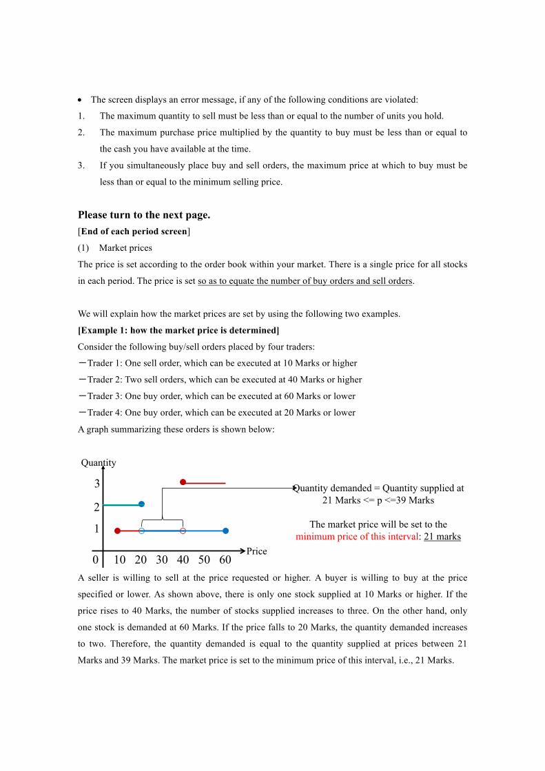
• The screen displays an error message, if any of the following conditions are violated:
1. The maximum quantity to sell must be less than or equal to the number of units you hold.
2. The maximum purchase price multiplied by the quantity to buy must be less than or equal to
the cash you have available at the time.
3. If you simultaneously place buy and sell orders, the maximum price at which to buy must be
less than or equal to the minimum selling price.
Please turn to the next page. [End of each period screen]
(1) Market prices
The price is set according to the order book within your market. There is a single price for all stocks
in each period. The price is set so as to equate the number of buy orders and sell orders.
We will explain how the market prices are set by using the following two examples.
[Example 1: how the market price is determined]
Consider the following buy/sell orders placed by four traders:
-Trader 1: One sell order, which can be executed at 10 Marks or higher
-Trader 2: Two sell orders, which can be executed at 40 Marks or higher
-Trader 3: One buy order, which can be executed at 60 Marks or lower
-Trader 4: One buy order, which can be executed at 20 Marks or lower
A graph summarizing these orders is shown below:
A seller is willing to sell at the price requested or higher. A buyer is willing to buy at the price
specified or lower. As shown above, there is only one stock supplied at 10 Marks or higher. If the
price rises to 40 Marks, the number of stocks supplied increases to three. On the other hand, only
one stock is demanded at 60 Marks. If the price falls to 20 Marks, the quantity demanded increases
to two. Therefore, the quantity demanded is equal to the quantity supplied at prices between 21
Marks and 39 Marks. The market price is set to the minimum price of this interval, i.e., 21 Marks.
Quantity demanded = Quantity supplied at 21 Marks <= p <=39 Marks
The market price will be set to the
minimum price of this interval: 21 marks Price�
Quantity�
3�
2
1�
0 10 20 30 40 50 60�
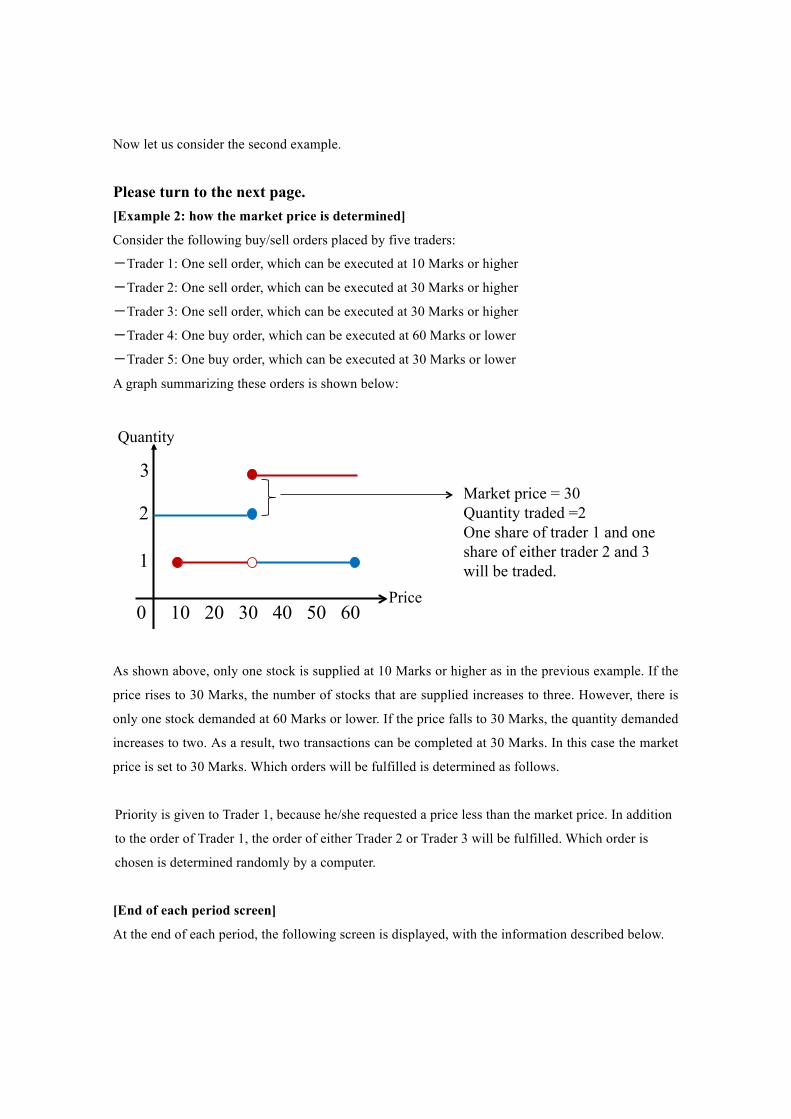
Now let us consider the second example.
Please turn to the next page. [Example 2: how the market price is determined]
Consider the following buy/sell orders placed by five traders:
-Trader 1: One sell order, which can be executed at 10 Marks or higher
-Trader 2: One sell order, which can be executed at 30 Marks or higher
-Trader 3: One sell order, which can be executed at 30 Marks or higher
-Trader 4: One buy order, which can be executed at 60 Marks or lower
-Trader 5: One buy order, which can be executed at 30 Marks or lower
A graph summarizing these orders is shown below:
As shown above, only one stock is supplied at 10 Marks or higher as in the previous example. If the
price rises to 30 Marks, the number of stocks that are supplied increases to three. However, there is
only one stock demanded at 60 Marks or lower. If the price falls to 30 Marks, the quantity demanded
increases to two. As a result, two transactions can be completed at 30 Marks. In this case the market
price is set to 30 Marks. Which orders will be fulfilled is determined as follows.
Priority is given to Trader 1, because he/she requested a price less than the market price. In addition
to the order of Trader 1, the order of either Trader 2 or Trader 3 will be fulfilled. Which order is
chosen is determined randomly by a computer.
[End of each period screen]
At the end of each period, the following screen is displayed, with the information described below.
Price�
Quantity�
3�
2�
1�
0 10 20 30 40 50 60�
Market price = 30 Quantity traded =2 One share of trader 1 and one share of either trader 2 and 3 will be traded.

(1) This shows the market price as explained previously.
(2) A positive value denotes the number of stocks you have purchased in the current period, while a
negative value denotes the number of stocks you have sold in the current period.
(3) This shows your cash holding after the transactions and dividend payments have been processed
for the current period.
(4) This is the number of stocks you currently hold.
(5) An explanation of Next Value is given on the next slide.
(6) The remaining time (maximum of 30 seconds) that this screen will be visible is displayed here.
After observing the information on the screen, press the “Continue” button (8). Once all of the
participants have pressed this button, the computer will display the next screen.
(7) By clicking this “Continue” button, you move to the next period.
Please turn to the next page. [Earning returns from dividends]
In the game, there are twenty periods in which you can submit your buy/sell orders and trade with
other traders in your market. You will also be offered a dividend of 12 Marks per stock based on the
number of stocks you have at the end of each period. Dividend income at the end of each period is
calculated as: 12 Marks × (number of stocks you hold).

[Next value]
As mentioned above, at the end of each period an amount is displayed as the “Next Value”. This
amount depicts the sum of the dividends per stock that will be offered in the remaining periods. For
example, consider Next Value at the end of the second period. There are 18 periods left. A dividend
of 12 Marks per stock will be offered 18 times. Thus, the Next Value is 12×18=216 Marks.
After period 20, a dividend is also paid according to your stock holdings. Your cash balance after
payment of the dividend for period 20 is the final amount you will earn in the game.
Turn to the next page to see a table of the Next Values. A copy of this table will be handed out
separately from the instructions. You should refer to this copy during the experiment as necessary.
Please turn to the next page. [Summary of ways to make a profit]
There are two ways of making a profit: (1) earning a profit margin, and (2) earning returns from
dividends. At the end of the experiment, 1 Mark will be converted into 1 Yen and paid out to you. In
addition to the aforementioned rewards, you will be offered 500 yen as a payment for participating
in the experiment.
[The instruction ends here]
Before stating the game, we will announce the following: Let’s start the game.
• There are six people in a market.
• All the people of the group are in this room. Each group consists of:
[6H/6L] only the top scorers or only the bottom scorers from the previous quiz.
[3H3L] three people in the top scorers and three people in the bottom scorers.
• Your rank, the top or the bottom, from the previous quiz is noted on the first screen.
• You will be given four stocks + 1040 Marks at the beginning of the game.
• After 20 periods, “You have completed the game” will appear on the screen. When this
appears, please click the continue button and wait for instructions.
Below we provide two examples of the screens used in known composition treatment informing
subjects regarding their relative rank based on the score of the quiz (top half or bottom half) and the
composition of group they belong to in the asset market experiment. The first one is for 6L and the
second on is for 3H3L.
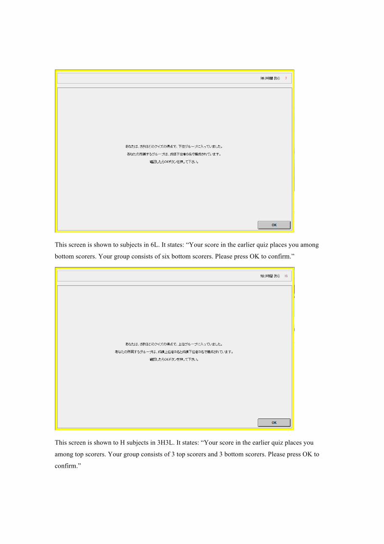
This screen is shown to subjects in 6L. It states: “Your score in the earlier quiz places you among
bottom scorers. Your group consists of six bottom scorers. Please press OK to confirm.”
This screen is shown to H subjects in 3H3L. It states: “Your score in the earlier quiz places you
among top scorers. Your group consists of 3 top scorers and 3 bottom scorers. Please press OK to
confirm.”

Documents De travail GreDeG parus en 2017GREDEG Working Papers Released in 2017
2017-01 Lauren Larrouy & Guilhem Lecouteux Mindreading and Endogenous Beliefs in Games2017-02 Cilem Selin Hazir, Flora Bellone & Cyrielle Gaglio Local Product Space and Firm Level Churning in Exported Products2017-03 Nicolas Brisset What Do We Learn from Market Design?2017-04 Lise Arena, Nathalie Oriol & Iryna Veryzhenko Exploring Stock Markets Crashes as Socio-Technical Failures2017-05 Iryna Veryzhenko, Etienne Harb, Waël Louhichi & Nathalie Oriol The Impact of the French Financial Transaction Tax on HFT Activities and Market Quality2017-06 Frédéric Marty La régulation du secteur des jeux entre Charybde et Scylla2017-07 Alexandru Monahov & Thomas Jobert Case Study of the Moldovan Bank Fraud: Is Early Intervention the Best Central Bank Strategy to Avoid Financial Crises?2017-08 Nobuyuki Hanaki, Eizo Akiyama, Yukihiko Funaki & Ryuichiro Ishikawa Diversity in Cognitive Ability Enlarges Mispricing in Experimental Asset Markets