documentos de economia y finanzas internacionales - … · during the period analyzed1, the...

DOCUMENTOS DE ECONOMIA YFINANZAS INTERNACIONALES

Asociación Española de Economía y Finanzas Internacionales

http://www.fedea.es/hojas/publicaciones.html

A PANEL COINTEGRATION APPROACH TO THE

ESTIMATION OF THE PESETA REAL EXNANGE RATE

Mariam Camarero

Cecilio Tamarit

November 2001

DEFI 01/08

A panel cointegration approach to theestimation of the peseta real exchange rate¤.

Mariam Camareroy

Jaume I University and FUNCAS

Cecilio TamaritUniversity of Valencia and FUNCAS

May 2001

Abstract

In this paper we estimate di¤erent speci…cations of a model for thedetermination of the bilateral real exchange rate of the peseta relativeto nine European Union members. The model is based on Meese andRogo¤ (1988) monetary approach as extended by MacDonald (1998).The applied econometric techniques are the recent panel cointegrationtests developed by Kao (1999), McCoskey and Kao (1998) and Pedroni(1999) for homogeneous and heterogeneous panels. The results arefavorable to a model containing relative productivities in tradables andnon-tradables and the real interest rate di¤erentials as explanatoryvariables.

Keywords: real exchange rate, European Monetary Union, panelcointegration

J.E.L. classi…cation: C33, F31.

¤We thank the …nancial support from the Fundación de las Cajas de Ahorros Confed-eradas (FUNCAS) and the Generalitat Valenciana research project GV99-135-8. MariamCamarero wants to acknowledge the funds provided by the project P1B98-21 from theJaume I University and Fundación Bancaja-Caixa Castelló. We also thank Suzanne Mc-Coskey and Chihwa Kao for some of the computer procedures to implement their tests.We are also indebted to Paco de Castro (Bank of Spain) and Román Arjona (OECD) fortheir help with the database. The article has also bene…ted from the comments of ananonymous referee. All remaining errors are ours.

yCorresponding author: Department of Economics. University Jaume I. Campus delRiu Sec. E-12071 Castellón (Spain). e-mail: [email protected].

1

1 Introduction.The aim of this paper is to study the main determinants of the Spanishpeseta real exchange rate during the ‡oat and the …rst years of EuropeanMonetary System (EMS) membership. The study of the real exchange rateis particularly relevant under the European Monetary Union (EMU), oncethe member countries have …xed their bilateral nominal exchange rates.

The peseta and the Spanish economy o¤er an interesting case study toanalyze the e¤ects of a process of opening to international competition ina context of regional integration. The Spanish experience can be relevantfor the assessment of the most adequate path to liberalization in emergingeconomies in the light of the European Union enlargement process.

Following the 1986 entry into the European Community, Spain dismantledthe majority of the restrictions on trade and on international capital ‡ows.The entry of foreign capital tended to appreciate the currency. Both domesticand foreign investment increased to accommodate the domestic market to thenew competitive conditions. A natural outcome of this opening process wouldbe the increase in productivity, mainly in the manufacturing sector, moreexposed to international competition. According to the Balassa-Samuelsone¤ect, this would cause an appreciation of the domestic currency.

During this same period, democracy in Spain introduced drastic changesin …scal policy, not only in the form of new income taxes and the VATimported from the European Community, but also with new orientations ofgovernment expenditure, that adopted an active and expansionary approach.

Finally, from 1986 (and specially since the 1989 entry in the EMS) theSpanish monetary authorities followed the so-called “competitive disin‡a-tion” strategy. In this framework, by keeping locked the nominal exchangerate, either the domestic prices are kept at the same (or lower) level as thecompetitors or a rise in the terms of trade causes a progressive loss of ex-ternal markets. This would provoke a more costly adjustment in terms ofrecession and, consequently, unemployment, but would …nally improve thecompetitiveness of the economy.

Bearing this strategy in mind, the Spanish authorities adopted, speciallyduring the period 1989-1992, a “hard peseta” policy in order to maintain thenominal exchange rate target. These measures also provoked a considerableappreciation of the real exchange rate of the peseta challenging, at the sametime, the whole strategy.

This paper investigates the factors, from the demand and the supply-sideof the economy that may have been in‡uential in the process of appreciationthat su¤ered the peseta during the eighties and the beginning of the nineties.Although there has been an increase in traded-goods productivity in Spain

2

during the period analyzed1, the Balassa-Samuelson e¤ect alone may notexplain all the peseta appreciation, so that the demand conditions shouldplay an important role in the Spanish economy. Hence, the study of thesefactors is of crucial importance for the future developments in the EMU,where another episode of real appreciation can be very dangerous for thecompetitive position of Spain, due to the absence of the nominal exchangerate as a policy instrument.

The empirical literature of real exchange rate determination has tradi-tionally obtained mixed evidence when using structural monetary models, sothat more eclectic formulations were also adopted in many empirical stud-ies. Recently, the traditional models have been revisited using cointegrationtechniques. However, the short spans of data available make it di¢cult toextract reliable conclusions. In this paper we have made an attempt to over-come these problems by applying new panel cointegration tests that allow usto extend the number of countries for a total of 20 years (from 1973 to 1992)in order to estimate the Spanish peseta bilateral real exchange rate relativeto 9 of its European Union partners.

The theoretical formulation adopted in this paper is based on MacDon-ald’s (1998) eclectic approach, that encompasses several structural modelstraditionally tested in the applied literature. This will permit to discrimi-nate between di¤erent models: from the Meese and Rogo¤ (1988) real interestdi¤erential model to the Rogo¤ (1992) intertemporal model based on pro-ductivity di¤erentials and relative public expenditure, and to the traditionalBalassa-Samuelson e¤ect.

The analysis will be performed with annual data for 10 European Unionmember countries for the period 1973-1992. Concerning the econometrictechniques, we use panel data cointegration methods, as proposed by Kao(1999), McCoskey and Kao (1998) and Pedroni (1999). These recent testscombine two approaches: …rst, the use of panel data that traditionally hasmeasured relationships between changes in exchange rates and changes inits determinants and, second, the use of cointegration techniques that mea-sures long-run relationships between the level of the exchange rate and thelevel of its determinants. The panel cointegration tests add, consequently,new insights to both the time series techniques and the cross-section studies,because previous cross-section analysis could not obtain long-run or equilib-rium models for the exchange rates, whereas the short spans of time-seriesdata available make di¢cult to extract reasonable estimates of the long-runcointegrating vectors2. This kind of tests may be useful for many cases inempirical work where there is a limited availability of data. Pooling thedata across individual members of a panel makes available more informationconcerning the cointegration hypothesis.

3

The paper is organized as follows: the second section reviews the theoret-ical and applied literature and presents the set of variables that may explainthe behavior of the peseta real exchange rate; the third section is devoted tothe discussion of the empirical results, and the fourth concludes.

2 Theoretical model: …nding the determinantsof the real exchange rate.

There is a wide academic agreement on the di¢culties commonly found inapplied work to model exchange rates. The monetary structural models ofthe seventies failed in the eighties when their forecasts were compared to asimple random walk model in the seminal paper of Meese and Rogo¤ (1983).A similar debate exists concerning the ful…llment of PPP. In both cases, neweconometric techniques, such as cointegration, have boosted a new generationof applied research in this …eld. However, the results are still not conclusiveand cannot give complete support to the traditional theories.

Trying to improve the results of the structural monetary models, Meeseand Rogo¤ (1988) studied the link between real exchange rates and real inter-est rate di¤erentials. Starting from a monetary model for the determinationof the real exchange rate, qt, this variable is de…ned as:

qt ´ et + p¤t ¡ pt (1)

where et is the logarithm of the domestic price of one unit of foreign currencyand pt and p¤t are the logarithms of domestic and foreign prices. Thus, whenthe real exchange rate increases, the domestic currency depreciates. Threeassumptions are made: …rst, that when a shock occurs, the real exchange ratereturns to its equilibrium value at a constant rate; second, that the long-runreal exchange rate, q̂t, is a non-stationary variable; …nally, that uncoveredreal interest rate parity is ful…lled:

Et(qt+k ¡ qt) = Rt ¡R¤t (2)

where Rt and R¤t are, respectively, the real domestic and foreign interest ratesfor an asset of maturity k:

Combining the three assumptions above, the real exchange rate can beexpressed in the following form:

qt = q̂t ¡ '(Rt ¡R¤t) (3)

where ' is a positive parameter larger than unity.

4

This leaves relatively open the question of which are the determinants ofq̂t, that is a non-stationary variable.

As Edison and Melick (1995) describe in their paper, the implementationof the empirical tests depends on the treatment of the expected real exchangerate derived from equation (3). The simplest model will assume that theexpected real exchange rate is constant3 , while the rest of the models will bespeci…ed using other determinants.

The second approach relaxes the assumption that the expected real ex-change rate is constant and try to explain it using additional variables. Thisapproach was …rst introduced by Hooper and Morton (1982) who modelledthe expected real exchange rate as a function of cumulated current account4.

An additional factor that has also been considered in the literature, to-gether with the previous determinants, is the productivity di¤erential5, con-sidered a major source of supply shocks a¤ecting the real exchange rate andalso a proxy variable for the Balassa-Samuelson e¤ect.

MacDonald (1998) follows a similar approach, dividing the real exchangerate determinants into two components: the real interest rate di¤erential anda set of fundamentals which include productivity di¤erentials, a demand sidebias, the e¤ect of relative …scal balances on the equilibrium real exchangerate, the private sector savings and the real price of oil.

Finally, Rogo¤ (1992), Obstfeld (1993) and Asea and Mendoza (1994)emphasize the role of …scal policy and other real variables (such as produc-tivity shocks, for example) in real exchange rate models, in contrast to themore traditional monetary approaches. Rogo¤ (1992) develops an intertem-poral model for exchange rate determination for the case of relatively closedcapital markets and factors that are not perfectly mobile across sectors.

Recently, the use of panel cointegration and unit root tests for panels ofcountries, such as in Chinn and Johnston (1996), Papell (1997), Anthony andMacDonald (1998), Cecchetti, Mark and Sonora (1998), Papell and Theodor-idis(1998), and MacDonald and Nagayasu (2000) have permitted to obtainmore encouraging results.

Therefore, in this paper, we will adopt an eclectic view closely related toMacDonald (1998) that includes the majority of the variables suggested inthe literature and we will estimate a model for the bilateral real exchangerate of the peseta relative versus a group of European Union partners usingpanel cointegration techniques.

MacDonald (1998) discusses a real exchange rate decomposition and de-…nes the real exchange rate in a similar fashion as in equation (1). He arrivesat the same expression that can be obtained from the Meese and Rogo¤(1988) monetary approach in equation (3). Thus, the actual equilibriumexchange rate has two components: the unobservable expectation of the ex-

5

change rate, q̂t; driven by the fundamentals and the real interest rate di¤er-ential, that may depend on other determinants.

Then, he further decomposes the real exchange rate in order to explainwhich are the group of fundamentals that may determine q̂t: He also proposesusing the cointegration framework to estimate the static relationship givenin expression (3).

Thus, a similar relationship to the one for the real exchange rate in equa-tion (1) may hold for the price of traded goods:

qTt ´ et + pT¤t ¡ pTt (4)

where a T superscript indicates that the variable is de…ned for traded goods.If the prices in (4) are composite terms, for qTt to be constant it has to beassumed that each of the goods prices which enters pTt has an equivalentcounterpart in pT¤t ; and the weights used to produce these composite pricelevels are the same.

Then, the general price indexes can be decomposed into traded and non-traded components as:

pt = (1 ¡ ®t)pTt +®tpNTt (5)

p¤t = (1¡ ®¤t)pT¤t + ®¤tp

NT¤t (6)

where the ®t denote the shares of nontradable goods sectors in the econ-omy, and are assumed to be time-varying, and NT denotes the non-tradedgoods. By substitution, MacDonald (1998) obtains an expression for thelong-run equilibrium real exchange rate, q̂t:

q̂t ´ qTt +®t(pTt ¡ pNTt ) ¡ ®¤t(pT

¤t ¡ pNT¤t ) (7)

Equation (7) permits to distinguish three potential sources of long-runreal exchange rate variability: …rst, nonconstancy of the real exchange ratefor traded goods, that may arise if the goods entering international trade areimperfect substitutes; second, movements in the relative prices of traded tonon-traded goods between the home and foreign country, due to productivitydi¤erentials in the traded goods sectors; …nally, di¤erences in the weightsused to construct the prices in the home and foreign country. However, theseweights will be considered constant, due to the di¢culties found to assessclearly their importance.

6

² The …rst factor considered by MacDonald (1998) relates to the relativeprice of traded to non-traded goods across countries, re‡ectedin the term (pTt ¡ pNTt )¡(pT¤t ¡pNT¤t ): The di¤erences may be a¤ectingthe relative price of non-traded goods, without necessarily a¤ecting therelative price of traded goods. He points out at two separate sets ofe¤ects. The …rst one would be the Balassa-Samuelson e¤ect, whilethe second one has to do with a demand-side bias towards non-tradedgoods.

According to the Balassa-Samuelson e¤ect, the nominal exchange ratemoves to ensure the relative price of traded goods is constant over time,so that qTt = c: However, productivity di¤erences in the production oftraded goods across countries can cause a bias into the overall exchangerate because productivity advances tend to concentrate in the tradedgoods sector. Then, if prices of goods are linked to wages, wages toproductivity and wages linked across industries, then the real exchangerate tends to appreciate for fast growing countries, even if the law ofone price holds for traded goods. Consequently, if the home countryis a fast growing economy, the term (pTt ¡ pNTt ) ¡ (pT¤t ¡ pNT¤t ) will benegative and this pushes q̂t below qTt :

The second e¤ect is related to the existence of a non-traded good biasin demand, that pushes the exchange rate away from its PPP levelde…ned using traded goods prices. If the income elasticity of demandfor non-traded goods is greater than unity, the relative price of non-traded goods will rise as income rises6. This e¤ect is reinforced by thefact that the share of government expenditure devoted to non-tradedgoods is larger than the share of private expenditure. Consequently,the demand bias will also tend to appreciate the real exchange rate.

² Despite the assumption made above in which qTt is constant, this factis not uncontroverted. In fact, the imperfect substitutability ofthe traded goods produced by industrial countries makes that theexisting price di¤erences may not be quickly arbitraged away. Accord-ing to MacDonald (1998), two factors may introduce variability in qTt :international di¤erences in savings and investment, and the real priceof oil.

Concerning the …rst factor, the relative price of non-traded goods is amajor determinant of the goods and nonfactor services component ofthe current account. The current account depends on the determinantsof national savings and investment, and the …scal balance is one keycomponent of national savings. Thus, private savings and the relative

7

…scal policies will in‡uence the equilibrium real exchange rate.

The literature on whether …scal policy consolidation strengthens orweakens the domestic currency is wide and has not solved the questionyet. In the traditional Mundell-Fleming model, a tightening of …scalpolicy increases national savings and, thus, lowers the domestic realinterest rate and depreciates the currency. In contrast, the portfoliobalance models and the asset market/balance of payments synthesismodel of Frenkel and Mussa (1988) consider that any interest earningson net foreign assets are o¤set by a corresponding trade imbalance.Hence, a permanent …scal consolidation will increase net foreign assetsand appreciate the long-run real exchange rate.

The other factor, private sector savings, tend to be very constant overtime. However, recent research, such as Masson et al (1993) suggestthat demographic factors may in‡uence di¤erences across countries inthe savings rate and, thus, a¤ect net foreign asset positions7.

Changes in the real price of oil can also have an e¤ect on the relativeprice of traded goods through their e¤ect on the terms of trade. Thisissue has already been used by Rogo¤ (1992) and by Amano and vanNorden (1998) who …nd that the real price of oil captures the majorityof the terms of trade shocks. For countries that are oil importers, thereal exchange rate would depreciate relative to oil producer countries8.

The eclectic model proposed by MacDonald encompasses, thus, other the-oretical models and empirical speci…cations widely used in the literature, asit has been summarized above. In particular, the intertemporal approachof Rogo¤ (1992) can be easily tested in this context.

² Rogo¤ (1992) model is based on the dynamic micro-foundation modelsof the real exchange rate. In contrast to the Balassa-Samuelson ap-proach, that considers that the characteristics of the individual’s util-ity function and the level of government consumption spending haveno e¤ect, he stresses the role of demand factors on the long-run behav-ior of real exchange rates. He considers that in open capital markets,and under imperfect factor mobility across sectors, agents can smooththeir consumption of tradables in the face of transitory traded goodsproductivity shocks. They cannot, however, smooth non-traded goodsproductivity shocks, normally caused by changes in government spend-ing, although if they are small traded-goods consumption smoothingwill lead to also smoothing the intra-temporal price of traded and non-traded goods. Thus, according to this model, productivity shocks as

8

well as changes in government spending will a¤ect the real exchangerate. However, he considers that only the second type of shocks mayhave permanent e¤ects. The critical issue that leads to predictions thatdo not support the traditional Balassa-Samuelson e¤ect is the existenceof imperfections in factor mobility across sectors. He …nds results fa-vorable to this approach for the case of Japan versus the German Markand the dollar.

Assuming that PPP holds for tradables, (so that as stated earlier qTt =c), Rogo¤ (1992) arrives to one expression of the type:

q̂t = ¡¡[(aTt ¡ a¤Tt)¡ ³N(aNt ¡ a¤Nt) + (³N ¡ 1)(gt ¡ g¤t ) + p0] (8)

where ¡ is a parameter related to the weights of the tradables andnon-tradables in the aggregate price index, (aTt ¡ a¤Tt) and (aNt ¡ a¤Nt)are the di¤erence in traded and non-traded goods productivity in thehome and foreign country, respectively, (gt¡g¤t ) is the di¤erence in realpublic expenditure to GDP between the two countries, ³N is the ratioof non-traded goods output to private non-traded goods consumptionand p0 represents the initial conditions from the intertemporal model.

This model also encompasses the Balassa-Samuelson model, if oneassumes that the parameter corresponding to government spending(³N ¡ 1) is zero.

Rogo¤ (1992) and Chinn (1997) use this expression to test the model,and the former also recommends to include the real price of oil toaccount for possible shifts in the terms of trade9.

Consequently, the models to be estimated in the paper will include com-binations of the following set of explanatory variables:

qt = f[(Rt ¡R¤t)(¡)

; (aT t ¡ a¤Tt)(¡)

; (aNt ¡ a¤Nt)(+)

; (gt ¡ g¤t )(¡=+)

]

where (Rt¡R¤t) is the real interest rate di¤erential, (aTt¡a¤Tt) and (aNt¡a¤Nt)the productivity di¤erentials in the traded and non-traded goods sectors, and(gt ¡ g¤t ) the di¤erence in the real public expenditure to GDP ratio.

To sum up, according to the expression above, an increase in the real in-terest rate di¤erential would cause the national currency to appreciate, fromthe assumptions of the monetary model summarized in equation (3): largerdomestic real interest rates will attract capitals and increase the demand forthe domestic currency.

9

Second, when domestic productivity in the traded goods sector increasesrelative to foreign productivity, there is a tendency of the domestic currencyto appreciate. Higher productivity in the tradables makes both labor andcapital more productive in that sector. Thus, the domestic output in thetraded sector also increases and the domestic …rms are able to reduce tradedprices. This will cause a reduction in the relative price of traded/non-tradedgoods and, as a result, the domestic currency appreciates in real terms.

In contrast, when the domestic productivity of non-tradables increasesrelative to foreign nontraded productivity, this induces workers to move fromthe traded to the more productive nontraded sector10, so that the domesticoutput of nontraded goods would increase. This makes it possible for thedomestic …rms to reduce the price of nontraded goods, so that the relativeprice of traded/non-traded goods will increase and the real exchange ratewould depreciate.

Finally, according to Rogo¤ (1992) public expenditure is biased towardsnon-traded goods, as it has been stated in the theoretical comments above.When the domestic real public expenditure to GDP is larger than the for-eign variable, the real exchange rate appreciates, due to the increase in non-tradables demand that causes the traded/non-traded price ratio to decrease.However, it should be also taken into account that a positive sign could alsobe found, according to Rogo¤ (1992) if public spending is not so clearly biasedtowards non-traded goods or, alternatively, if it is the traditional Mundell-Fleming model approach that works.

3 Empirical results.For the empirical analysis of the paper, the set of variables …nally chosen andcombined are the following:

rerit = f[drrit(¡)

; rprotrait(¡)

; rprontrait(+)

; dpexpit(+=¡)

] (9)

where rerit is the bilateral real exchange rate of the peseta based on CPIs;drrt is the real interest rate di¤erential, rprotrait and rprontrait are therelative productivity of the traded and non-traded goods in the domesticeconomy, respectively; and dpexpt is the di¤erential in real domestic publicexpenditure over GDP relative to the foreign country11.

We have considered 10 European Union countries, having excluded Lux-embourg, Greece, Ireland, Portugal and Finland due to problems of dataavailability. This permits us to obtain 9 relative variables, that give the …naldimension of the panel.

10

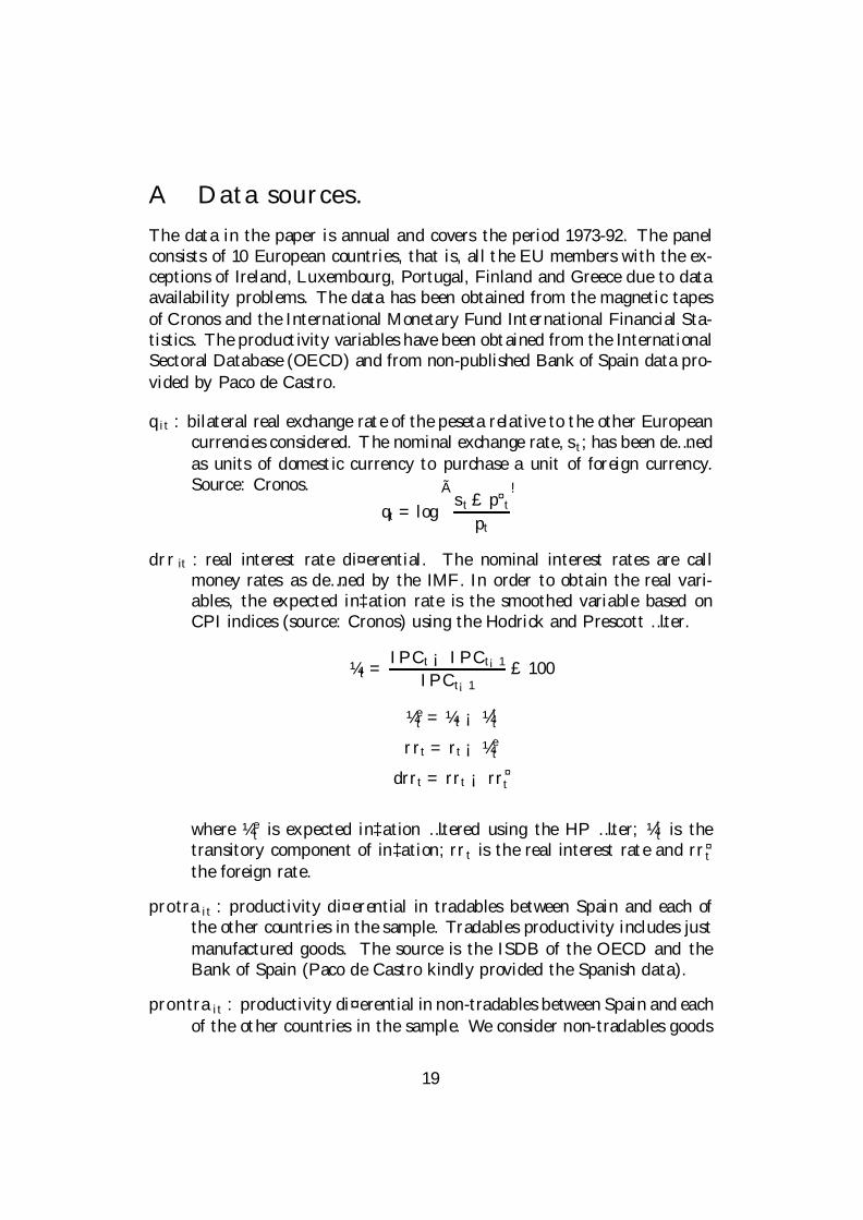
Previous to the study of the order of integration of the variables, we haveincluded in Figure 1 as an example the plots of the variables corresponding Insert

Figure1.

to the French case. From the observation of the graphs it can be derived thatthe relationships existing between the real exchange rate and its determinantsin the case of France closely follow what theory predicts.

There are some general trends that can be drawn from the graphicalinspection of the variables. First, the real exchange rate of the peseta ex-periences a progressive appreciation from the seventies, that became evensharper at the end of the eighties and beginning of the nineties to su¤er laterfour devaluations. Thus, the competitive position of the Spanish economyhas deteriorated continuously during the period analyzed. This deteriorationhas been only partially o¤set by the devaluations, although the ones in 1993and 1995 are beyond the sample period.

The time-path of traded-goods relative productivity is shown in the upperleft graph of Figure 1. The main pattern in tradables productivity di¤eren-tial with France is the steady growth of this variable that started at thebeginning of the eighties. Only at the end of the decade this di¤erentialslightly decreases. From the graph, its relation with the real exchange rateis generally negative for the period analyzed, although it may change at theend of the sample. In contrast, the lower left graph shows a very di¤erentpattern. The non-tradables productivity di¤erential seems to be positivelyrelated with the real exchange rate and no signi…cant changes in this behaviorcan be observed.

The upper right panel shows the time-path of the real interest rate dif-ferential and the dependent variable. In this case, the relation between thetwo series is negative, so that an increase in the real interest rate di¤erentialwould cause a real appreciation of the currency, as theory predicts.

Finally, in the lower right panel, the public expenditure di¤erential showsa positive slope. This trending behavior is due to the small size of the Spanishpublic sector at the beginning of the sample. Although public expenditurehas grown in all European countries, the Spanish one grew faster, due to itsinitial low level. It should be noted that the sharp increase experienced atthe end of the sample (versus France, in this case) is contemporaneous tothe real exchange rate appreciation of the end of the eighties. The negativerelationship observed in the graph would give support to the portfolio balanceinterpretation of the linkage between the two variables, as well as to thenegative relation postulated by the Rogo¤ (1992) model.

11

3.1 Panel cointegration.Previous to the cointegration analysis, the Kwiatkowski, Phillips, Smith andShin (1992) stationarity tests pointed at the non-stationarity of the vari-ables12.

In this section we apply various recent panel cointegration tests to themodel speci…ed in section 2. More speci…cally, the panel tests that have beenimplemented in this paper are: …rst, the DF and ADF-type tests proposedby Kao (1999) for the null hypothesis of no cointegration in homogeneousand heterogeneous panels; second, the panel cointegration test proposed byMcCoskey and Kao (1998) for the null of cointegration in heterogeneouspanels, based on Harris and Inder (1994) LM test developed for time series;…nally, we compare the results with the Pedroni (1999) heterogeneous paneland group tests13.

Due to the variety of explanatory variables that we have presented insection 2, we have proposed …ve di¤erent speci…cations that we test in thispaper, following the theoretical aspects discussed in the previous section:

M1: rerit = ®i+¯1irprotrait+¯2irprontrait (the Balassa-Samuelson model)

M2: rerit = ®i + ¯1irprotrait + ¯2irprontrait + ¯3idrrit (a partial version ofMacDonald’s model)

M3: rerit = ®i+¯1irprotrait+¯2irprontrait+¯3idpexpit (the Rogo¤ (1992)model)

M4: rerit = ®i + ¯1idrrit (the Meese and Rogo¤ (1988) model)

M5: rerit = ®i+¯1idpexpit (a restricted version of the Rogo¤ (1992) model)

The …rst model is a productivity-version14of the Balassa-Samuelson model,that is encompassed by models M2 and M3. The former is a speci…cationthat includes the Meese and Rogo¤ (1988) real interest di¤erential modeland the Balassa-Samuelson e¤ect, that are three of the variables proposedby MacDonald (1998). In the speci…cation M4 the simplest version of Meeseand Rogo¤ (1988), when the long-run real exchange rate is assumed to beconstant, is tested. Model M3 is the speci…cation presented in Rogo¤ (1992),whereas M5 is a restricted version of this model, where the productivitye¤ects are assumed not to be signi…cant.

These …ve models are tested for the 9 bilateral real exchange rates in thesample covering the period 1973-1992. In addition, for each model we will…rst assume that all the elements of the panel share the same slope para-meters. This implies that ¯11 = ¯12 = ::: = ¯19 = ¯1; the same restriction

12

would apply for the rest of the slope parameters in the …ve speci…cations.This is what we call the “homogeneous” model. If we relax this strong as-sumption and allow for the slope parameters to di¤er across the panel, wewill be testing the “heterogeneous” model. Consequently, we will presentboth cointegration tests and parameter estimates for the homogeneous andthe heterogeneous models. However, in the two types of models the interceptis allowed to be di¤erent for the cross-sections.

The ordering of the panel cointegration results is based on this duality. Intable 1 we …rst present the homogeneous Kao (1999) cointegration tests. Thenext table is devoted to the corresponding parameter estimates by OLS andbias corrected OLS. In table 3 we present the results of the panel and grouptests proposed by Pedroni (1999) for heterogeneous panels. Finally, tables4 and 5 contain the LM and ADF tests for cointegration in heterogeneouspanels for the …ve models speci…ed, table 6 presents some cointegration testsallowing for structural changes, and tables 7 to 10 the parameter estimatescorresponding to the …ve models.

3.1.1 Homogeneous panel cointegration tests and estimates.

The analysis of this section starts with the tests proposed by Kao (1999),based on the OLS residuals and assuming as the null hypothesis the absenceof cointegration. The DF ¤½ and the DF ¤t statistics are not dependent on thenuisance parameters, and are computed under the assumption of endogeneityof the regressors. Alternatively, he de…nes a bias-corrected serial correlationcoe¢cient estimate and, consequently, the bias-corrected test statistics andcalls themDF½ and DFt. Finally, he also proposes an ADF -type test for thenull of no cointegration. The results of applying these tests to the …ve modelspeci…cations are presented in table 1. For all the models and tests the null Insert

table1.

of no cointegration is rejected at 1%.Tables 2A and 2B show the OLS and bias corrected parameter estimates

Inserttables2Aand2B.

for all the speci…cations. The results of the two estimation techniques donot di¤er signi…cantly, with the exception of model M3. For the Balassa-Samuelson model presented …rst, that includes the two productivity di¤er-entials as explanatory variables, the parameters are highly signi…cant andexhibit the expected signs: negative for traded-goods productivity and pos-itive for the non-traded one. It should be noted, however, that the …rstparameter is larger in the bias-corrected estimates, whereas the second oneis smaller. Models M4 and M5 include as explanatory variables the real in-terest rate di¤erential and the relative public expenditure, respectively. Inother words, these two speci…cations include each one demand-side factor. Inthe two models and with the two estimators, the parameters have the correct

13

sign and are very signi…cant. Consequently, the four variables consideredseem to be adequate to explain the behavior of the real exchange rate duringthe period analyzed.

The two other speci…cations combine the productivity variables withdrr it (in model M2, the so-called MacDonald speci…cation) and with dp-expit (model M3, as in Rogo¤ (1992)). In the case of model M2, the homo-geneous speci…cation maintains the values of the coe¢cients’ estimates forthe productivity variables and the real interest rate di¤erential presents thecorrect sign. All the parameters are signi…cant both for the OLS and thebias-corrected estimates. The outcome is di¤erent in the case of model M3:the coe¢cient of government spending is negatively signed (being compati-ble with Rogo¤’s model and the portfolio approach) and signi…cant, whereasthe other two variables loose their explanatory power, specially in the biascorrected estimation.

As a conclusion, the M2 speci…cation seems to be, for the homogeneousmodel, the most representative of the relationships linking the real exchangerate and the supply and demand determinants. From this estimated relation,an increase in the traded-good sectors productivity in Spain relative to itscompetitors tends to appreciate the currency, whereas when this increaseoccurs in the non-traded good sectors, it follows a depreciation. Finally, fromthe demand-side, positive real interest rate di¤erentials cause an appreciationof the domestic currency.

3.1.2 Heterogeneous panel tests and estimates.

In this section we present the heterogeneous panel tests and estimates forthe …ve models speci…ed above using the Dynamic OLS (DOLS) estimationtechnique. The choice of this method relies on the Monte Carlo results of Kaoand Chiang (2000), who conclude that the OLS estimator has non-negligiblebias in …nite samples and the Fully Modi…ed (FMOLS) estimator does notimprove the results of the former in general. In contrast, the DOLS estimatorseems to be more promising for cointegrated panel regressions. The estimatedparameters are e¢cient and the t-statistics can be used for inference.

Pedroni (1999) proposed several tests for the null hypothesis of non-cointegration for panels with more than one regressor. We present in table3 the results of these tests for models M1, M2 and M3 (the models with two Insert

table3.

and three regressors) with intercepts but no trends, that is the speci…cationused here for the rest of the tests15. From the seven tests proposed by Pedroni(1999) four are called panel tests, that presume a common value for the unitroot coe¢cient, whereas the group tests allow for di¤erences in this parame-ter and give an additional source of potential heterogeneity. The tests are

14

di¤erent panel versions of the Phillips and Perron rho and t-statistic, as wellas panel versions of the ADF test. In fact, the parametric panel t-statisticis a panel cointegration version of the Levin and Lin (1993) panel unit roottest statistic, whereas the group equivalent is analogous to the Im, Pesaranand Shin (1997) group mean unit root statistic16 .

In a Monte Carlo experiment, Pedroni (1997) compares the performanceof the seven statistics in terms of size distortion and power, …nding …rst thatthe panel variance statistic was normally dominated by the other tests. Inaddition, the panel rho statistic exhibited the least distortions, whereas thegroup ADF had the worst and the group PP, panel PP and panel ADF fellin between. Concerning power and short samples (T=20, as in our case),the group ADF generally performs best, followed by the panel ADF and thepanel rho.

Bearing in mind these considerations, the results of the tests do notdi¤er signi…cantly between the three models analyzed. The null of non-cointegration is rejected at 1% for the three speci…cations using both thepanel and group ADF tests. However, it seems again that there is slightlymore support for model M2, that is, MacDonald’s extended version of Meeseand Rogo¤ (1988) model, than for the other two alternatives: the only testthat does not permit to reject the null for this model is the panel rho.

Tables 4 and 5 present the individual and panel LM and ADF tests for Inserttables4, 5and 6.

the heterogeneous case. It should be noted, before analyzing the results, thatin the …rst test the null hypothesis is cointegration, whereas in the ADF test,the null is absence of cointegration.

For the Balassa-Samuelson model (M1) the LM test by McCoskey andKao (1998) of the null of cointegration cannot be rejected either for theindividual countries or for the panel. The ADF test results, however, allowfor the rejection of the null at 5% for the panel, Austria and France, whereasthe cases of the Netherlands, Sweden and the UK are only rejected at 10%.For the rest, the absence of cointegration cannot be rejected. However, theMonte Carlo experiments reported by McCoskey and Kao (1999) point atthe larger power of the LM test if compared with other residual based testsfor cointegration in heterogeneous panels under the null of no cointegration(the average ADF test and Pedroni’s pooled tests).

This same pattern is present in models M2 and M3, where the LM tests,both individual and panel, support the cointegration hypothesis, whereas theevidence depends on the country for the ADF-type individual tests. However,the panel ADF tests reject in the two cases the null of no cointegration.

In contrast, the results for models M4 and M5, that only include demand-side variables, are less favorable to the existence of cointegration. The ADFindividual and panel tests do not permit to reject the absence of cointegra-

15

tion. The LM tests are more supportive of the cointegration hypothesis,although it is rejected for France and Italy in model M4.

Concerning the parameter estimates, we present the results for the …vemodels and the nine countries in tables 7 to 10. For model M1, the estimatedcoe¢cients for traded and non-traded relative productivity are presented intable 7. For the …rst variable, 7 out of 9 coe¢cients are signi…cant and 5 Insert

table7.

of them present the “correct” sign. For non-tradables, 4 are the signi…cantcoe¢cients, all of them positive, as the theory predicts. A similar patterncan be observed in table 8 for model M2. However, the number of signi…cant Insert

table8.

coe¢cients is now larger for the non-traded goods: 6 out of 9 and all of thempositive. Concerning the variable that has been added to this speci…cation,drr it, it is signi…cant for 6 countries and the coe¢cient is negative. Theparameter values are also very close to those obtained in the homogeneousestimation using OLS. Finally, in the speci…cation that includes the relativeproductivities and the public expenditure di¤erential (model M3 in table 9), Insert

table9.

there are only three signi…cant coe¢cients for the two productivities and onlyone for the …scal variable.

The other two model estimation results, presented in table 10, also sup- Inserttable10.

port the explanatory power of the two demand variables alone. In model M4,the real interest rate di¤erential is signi…cant in all the countries analyzedwith the only exception of Italy. In the case of dpexpit 5 out of 9 coe¢cientsare signi…cant, the exceptions being Sweden, Austria, Italy and the UK.

If we combine the test results and the estimated parameters, also theheterogeneous estimation seems to give support to model M2 as the mostcomplete and robust speci…cation from the …ve proposed17. In addition, itshould be emphasized that the parameters do not di¤er substantially acrossthe cross-sections, specially for the demand variables. This permits us toconclude that the performance of the real exchange rate of the peseta presentssimilar patterns for all the countries in the sample. Begum (2000) has foundsimilar parameter estimates for productivity di¤erentials in the case of theG-7 countries using the Johansen cointegration method.

3.2 Stability tests.As an additional test to the speci…cation …nally chosen (M2), we have appliedthe Gregory and Hansen (1996) tests for cointegration with regime changesthat have been computed for each individual country. The results are pre-sented in table 7, and should be interpreted together with the ADF testsresults in table 6 for the heterogeneous panel. Two tests and two modelshave been estimated: the ADF ¤ and the Z¤t tests in model C where thereis a change in the intercept, as well as in model C=T where a trend is also

16

present.According to Gregory and Hansen (1996), both the ADF and the ADF ¤

statistics test the null of no cointegration, so that rejection of the null usingany of them can be considered evidence in favor of cointegration and theexistence of a long-run relationship in the data. However, the ADF ¤ testshould be used more as a pre-test (previous to applying the conventionalones) than as speci…cation test. The Hansen (1992) is a better alternativefor speci…cation purposes, because the null hypothesis is the existence of ashift and the alternative is absence of this shift.

In addition, if the standard ADF statistic does not reject but the ADF ¤

does, this implies that structural change in the cointegrating vector may beimportant. Finally, if one …nds rejection from both tests, no inference aboutstructural change can be derived. The analysis should be complemented, inthis case, using the Hansen (1992) tests.

The results presented in table 7 point to the general rejection of thenull hypothesis of no-cointegration (if considered separately from the resultsof the individual ADF tests in table 6). In the case of Austria using thetwo speci…cations (models with intercept and with intercept and trend) andBelgium for model C, the null can only be rejected at 10%. In addition,the conventional results for model 2 (see the third column in table 6) do notallow the rejection of the null hypothesis. As Gregory and Hansen (1996)point out, rejection with any of the two tests would indicate the existence ofa long-run relation, and this is the general pattern observed in our results.

The empirical evidence found using theZ¤t is less favorable to the rejectionof the null hypothesis, with the exception of France, Sweden and the UK.

Therefore, if one considers the possibility of a structural change, thereis evidence of instabilities (as detected by the Gregory and Hansen (1996)statistics) that occur (according to the ADF¤ test results) at the end of theseventies or beginning of the eighties (being the exceptions France and Italy).Even if this was the case, the simultaneity of the majority of the instabilityepisodes would o¤set, at least partially, the economic consequences of possiblestructural changes.

4 Conclusions.In this paper we have studied the determinants behavior of the peseta realexchange rate in relation to 9 of its European partners for the period 1973-92, using panel cointegration tests. The theoretical formulation adopted inthis paper, based on MacDonald’s (1998) eclectic approach, has permittedto compare several structural models traditionally tested in the applied lit-

17

erature.The empirical methodology applied allows for di¤erent degrees of ‡exibil-

ity in the speci…cation of the long-run parameters linking the real exchangerate and its determinants. The panel results for the homogeneous modelsimpose the restriction of common slope coe¢cients for all the countries inthe sample, whereas the heterogeneous speci…cation allows for di¤erent esti-mates for every country. These two levels of results are crucial to discriminatebetween the models proposed.

To summarize the main empirical results, from models 1, 4 and 5, wecan derive that both supply and demand variables have been important inthe evolution of the peseta during the period studied. However, when com-bined, the speci…cation including the real interest rate di¤erential seems to bemore supported by the data than the one containing the di¤erence in publicexpenditure. Moreover, in the case of Spain, the two demand factors (con-tractionary monetary policy and expansionary …scal policy) appear to leadto an increase of real interest rates and to an appreciation of the currency.Thus, model 2, where only the real interest rate is included from the demand-side of the economy, along with the productivity variables, can be consideredthe most suitable one. These results can interpreted as giving support tothe Balassa-Samuelson model, although the non-tradables productivity dif-ferential is more signi…cant that its tradables equivalent. In addition, thehypotheses of Meese and Rogo¤ (1988) and Rogo¤ (1992) that stress theimportance of the demand-side of the economy for the determination of thereal exchange rate, is also supported by the data.

18

A Data sources.The data in the paper is annual and covers the period 1973-92. The panelconsists of 10 European countries, that is, all the EU members with the ex-ceptions of Ireland, Luxembourg, Portugal, Finland and Greece due to dataavailability problems. The data has been obtained from the magnetic tapesof Cronos and the International Monetary Fund International Financial Sta-tistics. The productivity variables have been obtained from the InternationalSectoral Database (OECD) and from non-published Bank of Spain data pro-vided by Paco de Castro.

q it : bilateral real exchange rate of the peseta relative to the other Europeancurrencies considered. The nominal exchange rate, s t; has been de…nedas units of domestic currency to purchase a unit of foreign currency.Source: Cronos.

qt = log

Ãst £ p¤tpt

!

drr it : real interest rate di¤erential. The nominal interest rates are callmoney rates as de…ned by the IMF. In order to obtain the real vari-ables, the expected in‡ation rate is the smoothed variable based onCPI indices (source: Cronos) using the Hodrick and Prescott …lter.

¼t =IPCt ¡ IPCt¡1

IPCt¡1£ 100

¼et = ¼t ¡ ¼ttrrt = rt ¡ ¼etdrrt = rrt ¡ rr¤t

where ¼et is expected in‡ation …ltered using the HP …lter; ¼tt is thetransitory component of in‡ation; rrt is the real interest rate and rr¤tthe foreign rate.

protra it : productivity di¤erential in tradables between Spain and each ofthe other countries in the sample. Tradables productivity includes justmanufactured goods. The source is the ISDB of the OECD and theBank of Spain (Paco de Castro kindly provided the Spanish data).

prontra it : productivity di¤erential in non-tradables between Spain and eachof the other countries in the sample. We consider non-tradables goods

19

all the sectors excluding manufacturing. The variable has been com-puted for each country as a weighted average where the weights dependon the relative importance of each sector in GDP.

dpexpit : public expenditure di¤erential. The government spending is cal-culated relative to GDP:

pext =pexntgdpnt

£ 100

where pexpnt is nominal public expenditure, whereas dpexpt = pext ¡pex¤t : The sources are IMF and Cronos.

20

Peseta/French Franc real exchange rateExplanatory variables

RERFR DLTRAFR

Rer and tradeables productivity

73 75 77 79 81 83 85 87 89 912.64

2.72

2.80

2.88

2.96

3.04

3.12

-0.05

0.00

0.05

0.10

0.15

0.20

0.25

0.30

RERFR DLNTRAFR

Rer and non-tradeables productivity

73 75 77 79 81 83 85 87 89 912.64

2.72

2.80

2.88

2.96

3.04

3.12

-0.060

-0.030

0.000

0.030

0.060

0.090

0.120

0.150

RERFR DRRFR

Rer and real interest rate differential

73 75 77 79 81 83 85 87 89 912.64

2.72

2.80

2.88

2.96

3.04

3.12

-12.5

-10.0

-7.5

-5.0

-2.5

0.0

2.5

5.0

RERFR DGFR

Rer and relative public expenditure

73 75 77 79 81 83 85 87 89 912.64

2.72

2.80

2.88

2.96

3.04

3.12

-6.5

-6.0

-5.5

-5.0

-4.5

-4.0

-3.5

-3.0

-2.5

-2.0

Figure 1:

B Graphs.

21

C Tables.Table 1

Homogeneous panel cointegration.Kao (1999) tests

Model speci…cations:

M1: rerit = ®i + ¯1rprotrait + ¯2rprontraitM2: rerit = ®i + ¯1rprotrait + ¯2rprontrait + ¯3drr it

M3: rerit = ®i + ¯1rprotrait + ¯2rprontrait + ¯3dpexpitM4: rerit = ®i + ¯1drrit

M5: rerit = ®i + ¯1dpexpit1973-1992

Test / Model M1 M2 M3 M4 M5DF½ -8.03¤¤¤ -10.29¤¤¤ -10.08¤¤¤ -9.08¤¤¤ -9.71¤¤¤

(0.00) (0.00) (0.00) (0.00) (0.00)DF t 3.64¤¤¤ 2.28¤¤ 2.44¤¤¤ 3.07¤¤¤ 2.67¤¤¤

(0.00) (0.01) (0.007) (0.001) (0.003)DF¤

½ -12.43¤¤¤ -15.75¤¤¤ -13.74¤¤¤ -14.96¤¤¤ -13.56¤¤¤

(0.00) (0.00) (0.00) (0.00) (0.00)DF¤

t -4.77¤¤¤ -5.89 -5.93 -5.09¤¤¤ -5.71¤¤¤

(0.00) (0.00) (0.00) (0.00) (0.00)ADF -3.97¤¤¤ -4.19¤¤¤ -5.43¤¤¤ -2.54¤¤¤ -5.09¤¤¤

(0.00) (0.00) (0.00) (0.005) (0.00)

Note: Two and three asterisks denote rejection of the null hypothesis ofno-cointegration at 5% and 1% respectively. The p-values are in parentheses.The test statistics are distributed as N(0,1).

22

Table 2A

Homogeneous panel OLS cointegration estimates

Dependent variable: rer it

Variables / Model M1 M2 M3 M4 M5rprotra -0.4848 -0.3561 -0.1437 — —

(-5.36) (-3.73) (-1.48)rprontra 0.4590 0.4586 0.2239 — —

(3.80) (3.91) (1.95)drr — -0.0074 — -0.0104 —

(-3.43) (-4.90)dpexp — — -0.0285 — -0.0335

(-6.51) — (-9.31)

TABLE 2B

Homogeneous panel OLS bias correctedcointegration estimates

Dependent variable: rer it

Variables / Model M1 M2 M3 M4 M5rprotra -0.6466 -0.4704 -0.1957 — —

(-4.37) (-3.73) (-1.51)rprontra 0.3234 0.3303 0.1035 — —

(2.04) (2.25) (0.75)drr — -0.0081 — -0.0130 —

(-3.33) (-4.74)dpexp — — -0.0341 — -0.0385

(-5.60) — (-6.82)

Note: t-values in parentheses. Signi…cant coe¢cients in bold.

23

Table 3

Pedroni (1999) cointegration testsfor heterogeneous panels.

Model with intercepts but without trends

Test/Model M1 M2 M3Panel variance test -1.42¤ -2.09¤¤¤ -1.35¤

(0.07) (0.01) (0.08)Panel ½ test -0.05 0.13 0.61

(0.47) (0.44) (0.26)Panel t-test (non-p.) -1.66¤¤ -2.17¤¤¤ -1.59¤¤

(0.04) (0.01) (0.05)Panel t-test (param.) -152.25¤¤¤ -208.19¤¤¤ -176.24¤¤¤

(0.00) (0.00) (0.00)Group ½ test 1.04 1.53¤ 2.13¤¤¤

(0.14) (0.06) (0.01)Group t-test (non-p.) -8.28 -9.65¤ -9.38

(0.11) (0.06) (0.11)Group t-test (param.) -4.02¤¤¤ -5.35¤¤¤ -4.98¤¤¤

(0.00) (0.00) (0.00)

Note: One, two and three asterisks denote rejection of the null hypothesisof non-cointegration at 10, 5 and 1% respectively.. All the tests have beennormalized, with the exception of the Group t-test in its non-parametricversion. The probabilities are in parentheses.

24

Table 4

Heterogeneous individual and panelLM cointegration tests results

1973-1992

Model M1 M2 M3 M4 M5Austria 0.025 0.008 0.009 0.079 0.044Belgium 0.109 0.004 0.006 0.046 0.039Denmark 0.057 0.013 0.016 0.062 0.111France 0.027 0.006 0.005 0.102 0.071Germany 0.021 0.006 0.009 0.338¤¤ 0.043Italy 0.051 0.005 0.018 0.326¤ 0.153Netherlands 0.022 0.007 0.010 0.134 0.071Sweden 0.034 0.006 0.005 0.134 0.123UK 0.009 0.004 0.005 0.209 0.140Panel test -2.86 -3.28 -3.24 -1.36 -2.23

Notes:(a) The tests and the models have been estimated using COINT 2.0 in

GAUSS 3.24 using the procedures provided by S. McCoskey and C. Kao.(b) The critical values at 1% (***), 5% (**), and 10% (*) for the LM

tests are the following: with one regressor, 0.549, 0.3202 and 0.233; with tworegressors, 0.372, 0.167, and 0.217; with three regressors, 0.275, 0.159 and0.120 (Harris and Inder, 1994). The critical value for the panel LM test is1.64.

25

Table 5

Heterogeneous individual and panelADF cointegration tests results

1973-1992

Model M1 M2 M3 M4 M5Austria -4.18¤¤ -4.71¤ -4.49¤ -3.51¤ -4.03¤¤

Belgium -2.07 -1.90 -3.33 -1.75 -3.07Denmark -3.25 -2.66 -3.26 -2.20 -3.11France -3.15 -3.53 -5.31¤¤¤ -2.82 -4.62¤¤¤

Germany -5.19¤¤¤ -3.96 -5.18¤¤¤ -1.17 -5.21¤¤¤

Italy -3.11 -3.11 -6.12¤¤¤ -1.63 -1.61Netherlands -3.85¤ -3.88 -4.32¤ -2.20 -3.92¤¤

Sweden -3.99¤ -3.91 -4.54¤¤ -0.60 -1.85UK -3.84¤ -4.37¤ -3.85 -2.10 -1.88Panel test -4.35¤¤ -4.20¤ -7.59¤¤¤ 1.74 -2.97

Notes:(a) The tests and the models have been estimated using COINT 2.0 in

GAUSS 3.24 using the procedures provided by S. McCoskey and C. Kao.(b) The lag order of the ADF tests is 1.(c) (b) The critical values at 1% (***), 5% (**), and 10% (*) for the

ADF tests are the following: with one regressor, -4.36, -3.80 and -3.51; withtwo regressors, -4.64, -4.15 and -3.84; with three regressors, -5.04, -4.48, and-4.19, and have been taken from Phillips and Ouliaris (1990).

26

Table 6Gregory and Hansen (1996) tests for a structural change

in the cointegration relationship

Model Model 2 (C) Model 3 (C/T)Country ADF¤ Tb Z¤t Tb ADF¤ Tb Z¤t Tb

Austria -5.03¤ 1982 -3.98 1978 -5.54¤ 1977 -4.62 1978(K=1)a (K=1)

Belgium -5.06¤ 1980 -5.07¤ 1979 -5.76¤¤ 1980 -4.30 1979(K=1) (K=1)

Denmark -6.27¤¤¤ 1978 -5.17¤ 1978 -6.24¤¤¤ 1978 -4.90 1978(K=1) (K=1)

France -6.36¤¤¤ 1987 -6.71¤¤¤ 1988 -6.61¤¤¤ 1984 -6.47¤¤¤ 1985(K=0) (K=2)

Germany -6.22¤¤¤ 1982 -4.33 1978 -5.70¤¤ 1982 -4.06 1978(K=1) (K=1)

Italy -5.37¤¤ 1989 -4.99 1989 -5.69¤¤ 1989 -5.28 1982(K=1) (K=1)

Netherlands -6.23¤¤¤ 1978 -4.96 1978 -6.16¤¤¤ 1978 -4.89 1978(K=1) (K=1)

Sweden -6.71¤¤¤ 1977 -7.05¤¤¤ 1977 -5.86¤¤ 1977 -6.04¤¤¤ 1977(K=0) (K=0)

UK -6.99¤¤¤ 1981 -7.29¤¤¤ 1979 -6.78¤¤¤ 1981 -6.94¤¤¤ 1980(K=2) (K=2)

Notes:(a) K stands for the number of lags in the AR for the ADF test.(b)The critical values have been obtained from Gregory and Hansen

(1996), table 1, and are for the case of three explanatory variables, -5.77,-5.28 and -5.02 at 1%, 5% and 10%, respectively in model 2 (C). For model 3(C/T), the critical values are -6.05, -5.57 and -5.33, at the same signi…cancelevels. Rejection of the null hypothesis is marked with asterisks.

(c) The GAUSS codes to compute the tests have been obtained from B.Hansen web-page.

27

TABLE 7

Panel cointegration.Individual DOLS parameter estimates

Model 1: 1973-92

Country intercepti rprotrai rprontraiAustria 2.096 0.168 2.428

(57.56) (0.18) (2.08)Belgium 1.004 -0.385 0.546

(6.57) (-0.18) (0.46)Denmark 2.795 -1.200 0.221

(31.61) (-2.65) (0.20)Germany 4.050 -0.820 4.308

(66.74) (-3.92) (3.16)France 3.013 -0.452 1.991

(152.38) (-3.67) (5.51)Italy -2.452 2.574 -0.125

(-37.09) (5.50) (-0.54)Netherlands 4.077 -2.739 1.459

(56.97) (-3.54) (2.09)Sweden 3.124 -1.034 0.504

(43.10) (-3.20) (1.55)UK 5.149 2.015 0.027

(140.68) (3.60) (0.07)

Note:(a) t-Students are reported in parentheses. Signi…cant coe¢cients in bold.

28

TABLE 8


Model 2. 1973-92

Country intercepti rprotrai rprontrai drr iAustria 2.092 3.769 -1.877 -0.031

(62.50) (1.56) (-0.58) (-1.35)Belgium 0.829 -0.334 1.072 -0.061

(21.38) (-0.72) (3.88) (-11.58)Denmark 2.405 0.552 1.948 -0.045

(13.71) (0.56) (1.75) (-2.09)Germany 3.822 0.367 3.651 -0.035

(83.73) (1.80) (5.81) (-5.77)France 2.935 -0.334 1.600 -0.014

(87.70) (-3.27) (4.36) (-2.00)Italy -2.517 2.372 0.127 0.007

(-40.56) (4.94) (0.61) (0.92)Netherlands 2.907 -0.200 2.596 -0.058

(22.49) (-0.11) (3.54) (-2.05)Sweden 2.907 -0.208 0.931 -0.035

(22.49) (-0.39) (2.77) (-2.58)UK 5.126 2.273 -0.129 0.009

(71.05) (2.19) (-0.25) (0.35)


29

Table 9


Model 3. 1973-92Country intercepti rprotrai rprontrai dpexpiAustria 2.161 -0.885 2.666 0.003

(4.95) (-0.28) (0.54) (0.03)Belgium 1.005 0.885 1.567 -0.030

(10.28) (0.55) (1.72) (-1.29)Denmark 2.721 -0.698 1.004 -0.001

(1.69) (-0.39) (0.43) (-0.01)Germany 3.497 0.451 2.227 -0.080

(6.18) (0.40) (0.77) (-1.20)France 2.353 0.270 0.007 -0.114

(3.46) (0.35) (0.00) (-0.97)Italy -2.437 3.364 -0.511 -0.052

(-12.48) (4.64) (-1.21) (-1.15)Netherlands 3.778 2.215 2.179 -0.046

(49.26) (4.22) (12.86) (-3.42)Sweden 3.579 -0.705 1.887 0.045

(14.05) (-2.48) (2.78) (2.11)UK 4.936 2.255 -0.388 -0.026

(6.05) (0.72) (-0.143) (-0.31)


30

TABLE 10


Model 4 and model 5.1973-92

MODEL M4 M5Country intercepti drr i intercept i dpexpit

Austria 2.097 -0.012 2.062 -0.026(86.66) (-2.03) (22.79) (-1.63)

Belgium 1.017 -0.045 1.107 -0.032(48.70) (-6.97) (16.72) (-3.08)

Denmark 2.722 -0.019 2.342 -0.038(97.76) (-3.60) (13.34) (-2.60)

Germany 4.040 -0.021 3.706 -0.060(155.31) (-3.36) (45.88) (-5.46)

France 2.903 -0.026 2.526 -0.084(126.17) (-2.61) (29.37) (-5.58)

Italy -2.491 -0.004 -2.461 0.006(-85.96) (-0.42) (-17.67) (0.09)

Netherlands 3.894 -0.033 3.936 -0.040(120.71) (-3.63) (73.52) (-5.64)

Sweden 2.894 -0.041 2.507 -0.035(142.27) (-6.09) (15.87) (-3.05)

UK 5.286 0.062 5.151 -0.020(208.32) (3.20) (32.97) (-0.93)


31

References[1] Amano, R.A. and S. van Norden “Oil prices and the rise and fall of the

US real exchange rate”, Journal of International Money and Finance 17(1998): 299-316.

[2] Anthony, M. and R. MacDonald “On the mean-reverting properties oftarget zone exchange rates: some evidence for the ERM”, EuropeanEconomic Review 42 (1998): 1493-1523.

[3] Asea, P. and E. Mendoza “Do long-run productivity di¤erentials explainlong-run real exchange rates?”, Review of International Economics 2(1994): 244-267.

[4] Baxter, M. “Real exchange rates and real interest di¤erentials. Havewe missed the business-cycle relationship?”, Journal of Monetary Eco-nomics 33 (1994): 5-37.

[5] Begum, J. “Real exchange rates and productivity: Closed-form solutionsand some empirical evidence”, International Monetary Fund WorkingPaper, WP/00/99 (2000).

[6] Campbell, J.Y. and R.H. Clarida “The dollar and real interest rates”,Carnegie-Rochester Conference Series on Public Policy, 24 (1987) ,A.Meltzer and K. Brunner (eds.), North Holland, Amsterdam.

[7] Campbell, J.Y. and P. Perron “Pitfalls and Opportunities: What Macro-economists Should Know about Unit Roots”, in O.J. Blanchard and S.Fischer (eds.), NBER Macroeconomics Annual 1991, The MIT Press(1991): 141-201.

[8] Cecchetti, S.G., N.C. Mark and R. Sonora “Price level convergenceamong United States Cities: lessons for the European Central Bank”,Oesterreichische Nationalbank Working Paper 32 (1998).

[9] Chiang, M. H. and C. Kao “Nonstationary Panel Time Series using NPT1.1. A User Guide”, Center for Policy Research, Syracuse University(2000).

[10] Chinn, M. “Paper pushers or paper money? Empirical assessment of…scal and monetary models of exchange rate determination”, Journal ofPolicy Modelling vol. 19 (1997): 51-78.

32

[11] Chinn, M. and L. Johnston “Real exchange rate levels, productivity anddemand shocks: evidence from a panel of 14 countries”, NBER WorkingPaper 5709 (1996).

[12] De Grauwe, P Teoría de la Integración Monetaria. Celeste Editores,Madrid (1994).

[13] De Gregorio, J. and H.C. Wolf “Terms of trade, productivity, and thereal exchange rate”, NBER Working Paper n. 4807 (1994).

[14] Edison, H.J. and W.R. Melick “Alternative approaches to real exchangerates and real interest rates: three up and three down”, InternationalFinance Discussion Papers, n. 518, Board of Governors of the FederalReserve System (1995).

[15] Edison, H.J. and B.D. Pauls “A re-assessment of the relationship be-tween real exchange rates and real interest rates: 1974-1990”, Journalof Monetary Economics 31 (1993): 165-87.

[16] Faruqee, H. “Lung-run determinants of the real exchange rate: A stock-‡ow perspective”, IMF Sta¤ Papers 42 (1995): 80-107.

[17] Frenkel, J. and J. Mussa “Exchange rates and the balance of payments”,in R. Jones and P. Kenen (eds.), Handbook of International Economics3 (1988). Amsterdam, North Holland.

[18] Gregory, A. W. and B.E. Hansen “Residual-based tests for cointegrationin models with regime shifts”, Journal of Econometrics 70 (1996), 99-126.

[19] Hansen, B.E. “Tests for parameter instability in regressions with I(1)processes”, Journal of Business and Economic Statistics 10 (1992): 321-335.

[20] Harris, D. and B. Inder “A test of the null hypothesis of cointegration”,in Nonstationary Time Series Analysis and Cointegration, Hargreaves,Colin P. Ed., Oxford University Press, New York (1994).

[21] Hooper, P. and J. Morton “Fluctuations in the dollar: a model of nom-inal and real exchange rate determination”, Journal of InternationalMoney and Finance 1 (1982), 39-56.

[22] Im, K., M.H. Pesaran and Y. Shin “Testing for unit roots in heteroge-neous panels”, Department of Applied Economics, University of Cam-bridge (1995).

33

[23] Kao, C. “Spurious regression and residual-based tests for cointegrationin panel data”, Journal of Econometrics 90 (1999): 1-44.

[24] Kao, C. and M.H. Chiang “On the estimation and inference of a cointe-grated regression in panel data”, Advances in Econometrics 15 (2000),forthcoming.

[25] Kwiatkowski, D., P.C.B. Phillips, P. Schimidt, and Y. Shin “Testingthe null hypothesis of stationarity against the alternative of a unit root:How sure are we that economic time series have a unit root?”, Journalof Econometrics 54 (1992): 159.78.

[26] Lane, P. R. and G.M. Milesi-Ferretti “The transfer problem revisited:Net foreign assets and real exchange rates”, CEPR International Macro-economics Discussion Papers, n. 2511 (July 2000).

[27] Levin, A. and C. Lin “Unit root tests in panel data: New results”,Discussion Paper 93-56, University of California, San Diego (December1993).

[28] MacDonald, R. “What determines real exchange rates? The long andthe short of it”, Journal of International Financial Markets, Institutionsand Money 8 (1998): 117-153.

[29] MacDonald, R. and J. Nagayasu “The long-run relationship betweenreal exchange rates and real interest di¤erentials: A panel study”, IMFSta¤ Papers 47 (2000): 116-128.

[30] Masson, P. J. Kremers and J. Horne “Net foreign assets and inter-national adjustments: the United States, Japan and Germany”, IMFWorking Paper 93/33 (1993).

[31] McCoskey, S. and C. Kao “A Monte Carlo comparison of tests for coin-tegration in panel data”, mimeo, Syracuse University (1998).

[32] McCoskey, S. and C. Kao “Comparing panel data cointegration testswith an application of the Twin De…cits problems”, working paper, Cen-ter for Policy Research, Syracuse University (1999).

[33] Meese, R. and K. Rogo¤ “The out-of-sample failure of empirical ex-change rate models: sampling error or misspeci…cation?” in Frenkel,J.A. (ed.), Exchange rates and International Macroeconomics (1983):67-105.

34

[34] Meese, R. and K. Rogo¤ “Was it real? The exchange rate-interest dif-ferential relation over the modern ‡oating-rate period”, The Journal ofFinance 43 (1988): 933-48.

[35] Obstfeld, M. “Model trending real exchange rates”, CIDER WorkingPaper C93-011, University of California at Berkeley (1993).

[36] Papell, D.H. “Searching for stationarity: Purchasing power parity underthe current ‡oat”, Journal of International Economics 43 (1997), 313-332.

[37] Papell, D.H. and H. Theodoridis “Increasing evidence of purchasingpower partiy over the current ‡oat”, Journal of Interantional Moneyand Finance 17 (1998): 41-50.

[38] Pedroni, P. “Panel Cointegration; Asymptotic and Finite Sample Prop-erties of Pooled Time Series Tests, with an Application to the PPPHypothesis: New Results”, working paper, Indiana University (April1997).

[39] Pedroni, P. “Critical Values for Cointegration Tests in HeterogeneousPanels with Multiple Regressors”, Oxford Bulletin of Economics andStatistics 61 (1999): 653-678.

[40] Phillips, P.C.B. and S. Ouliaris “Asymptotic properties of residual basedtests for cointegration”, Econometrica 58 (1990): 165-193.

[41] Raymond, J.L. and B. García-Greciano “El tipo de cambio real de lapeseta y productividad. Una visión de largo plazo”, Revista de EconomíaAplicada V (1997): 31-47.

[42] Rogo¤, K. “Traded goods consumption smoothing and the random walkbehaviour of the real exchange rate”, Bank of Japan Monetary and Eco-nomic Studies 10 (1992): 783-820.

[43] Strauss, J. “The cointegrating relationship between productivity, real ex-change rates and purchasing power parity”, Journal of Macroeconomics18 (1996): 299-313.

[44] Wu, J. L. “A re-examination of the exchange rate-interest di¤erentialrelationship: evidence from Germany and Japan”, Journal of Interna-tional Money and Finance 18 (1999): 319-336.

35

End notes1According to De Grauwe (1994), the average annual productivity growth ofmanufacturing in Spain during the eighties was 3.5%, compared to 2.5% inFrance, 3.0% in Germany and 4.2% in Italy.

2Raymon and García-Greciano (1997) have estimated a model for thepeseta real exchange rate using traditional panel methods.

3See, for example, Campbell and Clarida (1987), Meese and Rogo¤ (1988),Baxter (1994) and MacDonald and Nagayasu (2000).

4See Edison and Pauls (1993), Edison and Melick (1995) and Wu (1999).5Strauss (1996), De Gregorio and Wolf (1994) and Lane and Milesi-

Ferretti (2000) have studied this type of speci…cation.6That is, as income rises, the demand for services increases.7In the empirical part of the paper we will not consider this variable, that

turned out to be stationary.8Initially, we introduced the real oil prices in some of the speci…cations

presented later in the paper, but the variable was not signi…cant (or it wasbut only for one or two of the countries in the sample), so that it was …nallydiscarded.

9It has been assumed that the terms of trade are constant, so that theinclusion of the real price of oil permits to consider a possible source ofexogenous shocks in the model.

10If one accounts for the assumption of imperfect mobility across sectorsas in Rogo¤ (1992), this e¤ect would be weaker.

11See appendix A for further details about the de…nition of the variables.12These results have been omitted but are available from the authors upon

request.13The econometric procedures necessary to calculate the tests and esti-

mate the coe¢cients have been kindly provided by S. McCoskey and C. Kao.In addition, we have used the program NPT 1.1 (see Chiang and Kao, 2000).All computations have been made in GAUSS 3.24.

14This model can also be tested using relative prices of traded and non-traded goods.

15Two other speci…cations, without constant and with constant and trendhad been estimated, and are available upon request. The results did not di¤erfrom the ones presented in the text.

16See Pedroni (1999) for a detailed description of these statistics.17Problems related to data availability for the breakdown of traded and

non-traded goods productivity did not allow us to expand the sample periodbeyond 1992. However, in a previous version of the paper where we consid-ered aggregate productivity instead, the sample ended in 1997. The results

36

were also favorable to a speci…cation that included, as the main explana-tory variables, the real interest rate di¤erential and productivity di¤erentials.Thus, from this evidence, we think that this pattern in the behavior of thepeseta real exchange rate may have been mantained up to 1997.

37

documentos de economia y finanzas internacionales - … · during the period analyzed1, the...

Documents