Download - Climate Modeling

Climate ModelingClimate Modeling
Inez FungDept of Earth and Planetary Science
Dept of Environmental Science, Policy and Management
UC Berkeley

mass
energy
water vapor
momentum
)(
...),,,(
,...),(
)(
),(;
0)(
)(ˆ12
2
qonCondensatiEvapqutq
GHGCOqTfLW
aerosolscloudsfSW
TLHSHLWSWTutT
qTfRTp
ut
uFkgpuuutu
ℑ+−=∇•+∂∂
==
ℑ++++=∇•+∂∂
==
=•∇+∂∂
ℑ+++∇−=×Ω+∇•+∂∂
r
bbr
r
rrrrrr
ρρ
ρρ
ρ
Atmosphere
ℑ convective mixing

Ocean
momentum
mass
energy
salinity )()(
)(
),(;0
0
12
00
03
03
2
00
2222
sPEz
ssu
ts
TQTutT
sTfgzp
zw
u
Fpuuutu
ℑ+−Δ
=∇•+∂∂
ℑ+=∇•+∂∂
=+∂∂
−=
=∂∂
+•∇
++∇−=×Ω+∇•+∂∂
ρ
ρρ
τρ
r
r
r
rrrrrr

Earth’s Energy Balance, with GHG
COCO22, H, H22O, GHGO, GHG
Earth
70
95114
23
7
50 absorbed by sfc
Sun
30
20 absorbed by atm
100

Climate Processes
• Radiative transfer: solar & terrestrial
• phase transition of water
• Convective mixing• cloud microphysics• Evapotranspirat’n• Movement of heat
and water in soils

Climate Feedbacks
Warming
Decrease snow cover;Decrease reflectivity of surfaceIncrease absorption of solar energy
Increase cloud cover;Decrease absorption of solar energy
Evaporation from ocean,Increase water vapor in atmEnhance greenhouse effect

Observed Warming greatest at high
latitudes
Amplification of warming due to decrease of albedo (melting of snow and ice)

Will cloud cover increase or decrease with warming? [models: decrease; warm air can hold more moisture; +ve feedback]
A B + water vapor + longwave abs Warming
A C + water vapor + cloud cover + longwave abs - shortwave abs
275 280 285 290 295 3000
5
10
15
20
25
30
35
40
1 2 3 4 5 6
Temperature (K)
Sat
urat
ion
Vap
or P
ress
ure
(mb)
A
B
Cliquid
vapor

“Externally Forced” climate variability: Milankovitch Cycles (Orbital Variations)
Co-Variations of CO2 and Climate
100
150
200
250
300
0 50 100 150 200 250 300 350 400 450
Thousand Years Before Present
CO2 (ppmv)
-10
-5
0
5
10
Te
mp
era
t ur e
De
pa r
t ur e
(K
)
120,000 yr
Last Glacial Max

e.g.•El-Nino / Southern Oscillation
•Instability of the air-sea system in the equatorial pacific
•Irregular
•2-7 year
“Internal” Variability of the Climate System
1885
1995
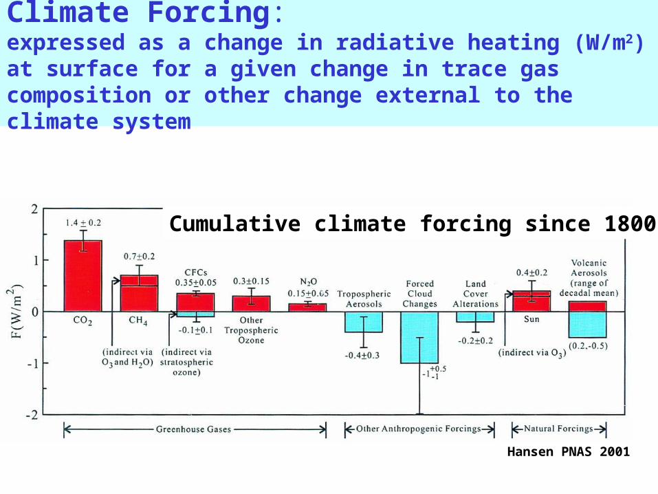
Climate Forcing: expressed as a change in radiative heating (W/m2) at surface for a given change in trace gas composition or other change external to the climate system
Hansen PNAS 2001
Cumulative climate forcing since 1800
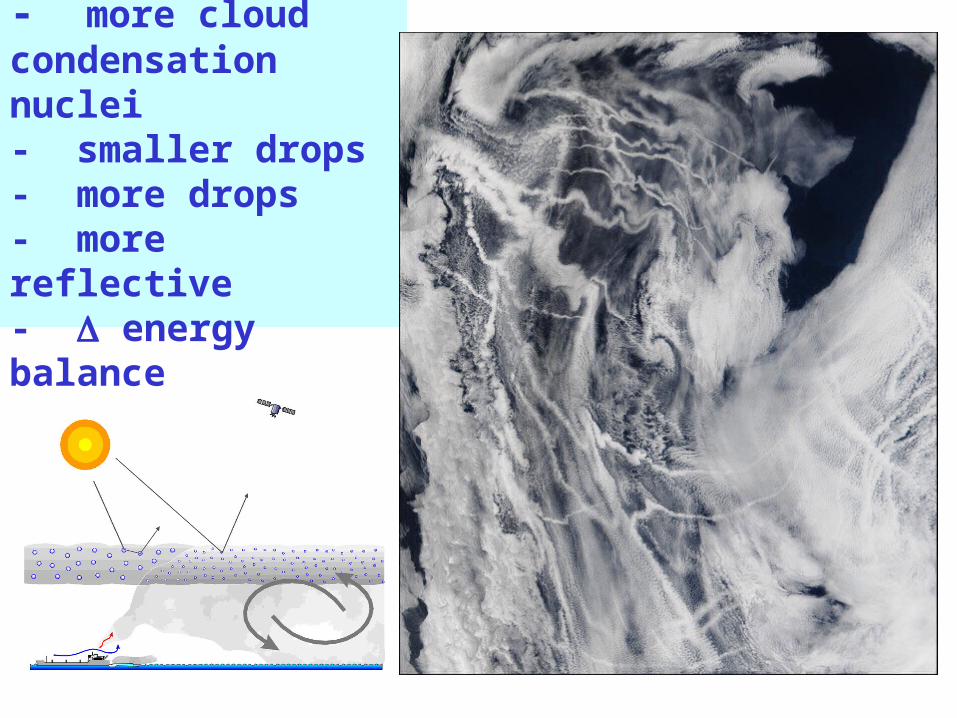
Ship Tracks:- more cloud condensation nuclei- smaller drops- more drops- more reflective- Δ energy balance

Numerical Weather Prediction ( ~ days)
Initial Conditions
t = 0 hr
Prediction t = 6 hr 12 18 24
1st Numerical Weather Prediction Experiment • Charney, Fjortoft and von Neumann (1950, Tellus) • Barotropic Vorticity Eqn • ENIAC computer (10 word memory) • 1 layer over N America
Now: Operational forecasts (model validation in ~days); require model + initial conditions (obs atm)

Seasonal Climate Prediction ( ~ months) ( El – Nino Southern Oscillation )
{ Initial Conditions}
Atm + Ocn t = 0
{Prediction}
t = 1 mo 2 3
• Coupled atmosphere-ocean instability• Require observations of initial states of both atm & ocean, esp. Equatorial Pacific• Cane & Zebiak ( 1986, 1987)• {Ensemble} of forecasts • Forecast statistics (mean & variance) – probability• Now – experimental forecasts (model testing in ~months)

Climate Models Capture Magnitude and Timing of Recent Warming
Meehl et al. 2006; Hansen et al. 2005

Published by AAAS
G. A. Meehl et al., Science 305, 994 -997 (2004)
Fig. 3. Height anomalies at 500 hPa (gpm) for the 1995 Chicago heat wave (anomalies for 13 to 14 July 1995 from July 1948 to 2003 as base period), from NCEP/NCAR
reanalysis data (A) and the 2003 Paris heat wave (anomalies for 1 to 13 August 2003 from August 1948 to 2003 as base period), from NCEP/NCAR reanalysis data (B)

Published by AAAS
G. A. Meehl et al., Science 305, 994 -997 (2004)
Fig. 4. Height anomalies at 500 hPa (gpm) for events that satisfy the heat wave criteria in the model in future climate (2080 to 2099) for grid points near Chicago (A)
and Paris (B), using the same base period as in Fig

21stC warming depends on CO2 increase
20thC stabilizn:CO2 constant at 380 ppmv for the 21stC
21thC “Business as usual”:CO2 increasing 380 to 680 ppmv
Meehl et al. (Science 2005)


