
ENGM 745 Forecasting for Business & Technology
Paula Jensen
South Dakota School of Mines and Technology, Rapid City
3rd Session 2/01/12: Chapter 3 Moving Averages and Exponential Smoothing
Agenda & New Assignment
ch3(1,5,8,11) Business Forecasting 6th Edition
J. Holton Wilson & Barry KeatingMcGraw-Hill

Moving Averages & Exponential Smoothing All basic methods based on
smoothing 1. Moving averages 2. Simple exponential smoothing 3. Holt's exponential smoothing 4. Winters' exponential smoothing 5. Adaptive-response-rate single
exponential smoothing

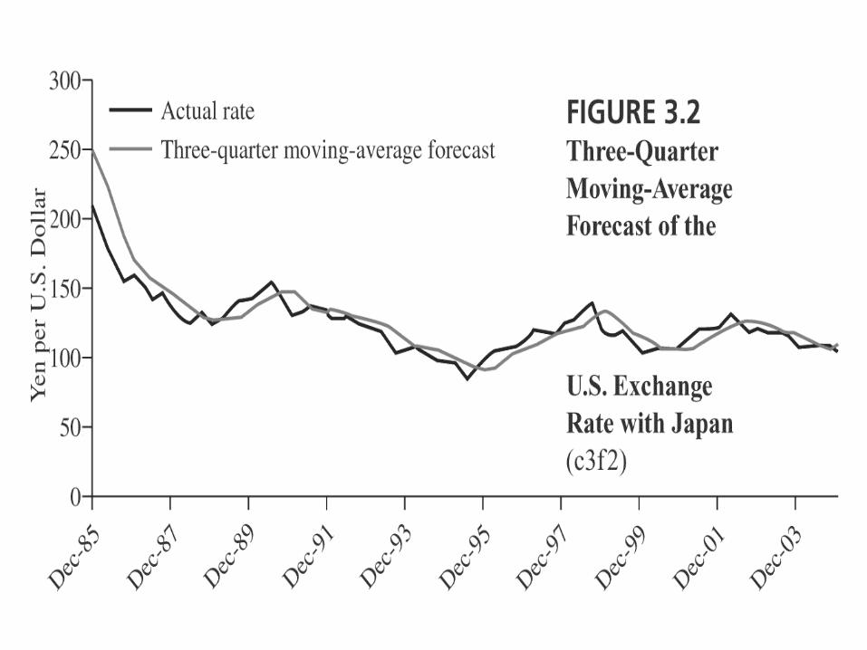
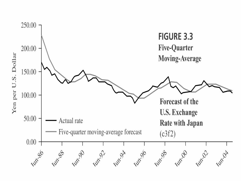
Moving Averages Ex. “Three Quarter Moving Average”
(1999Q1+1999Q2+1999Q3)/3 =Forecast for 1999Q4
Slutsky-Yule effect: Any moving average could appear to be acycle, because it is a serially correlated set of random numbers.
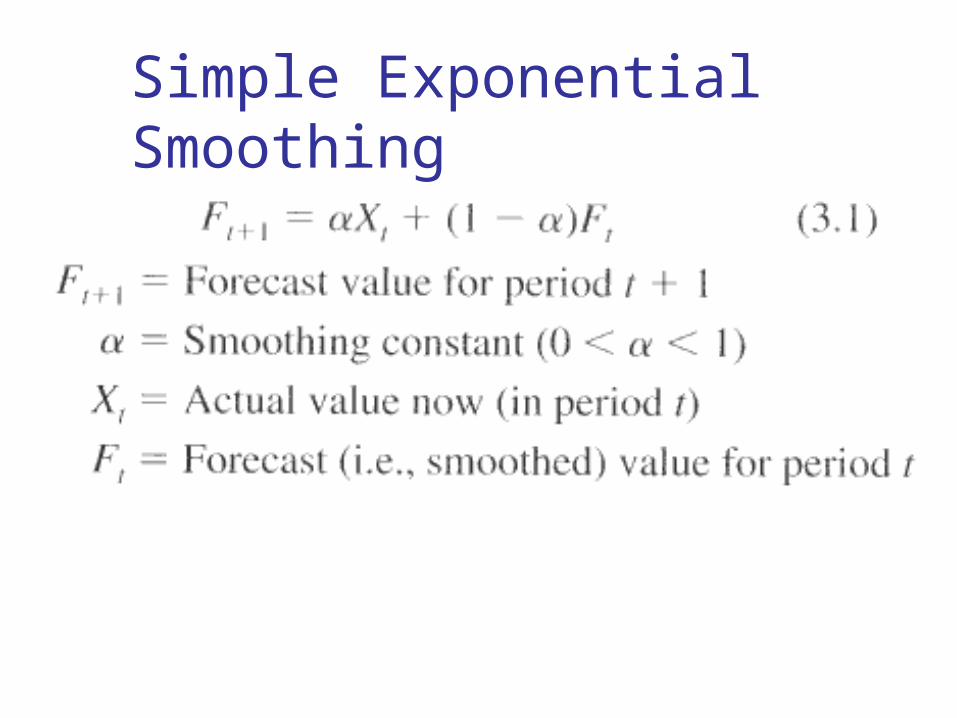
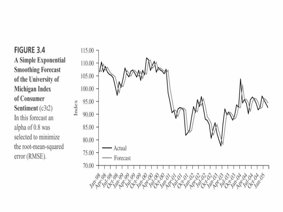
Simple Exponential Smoothing
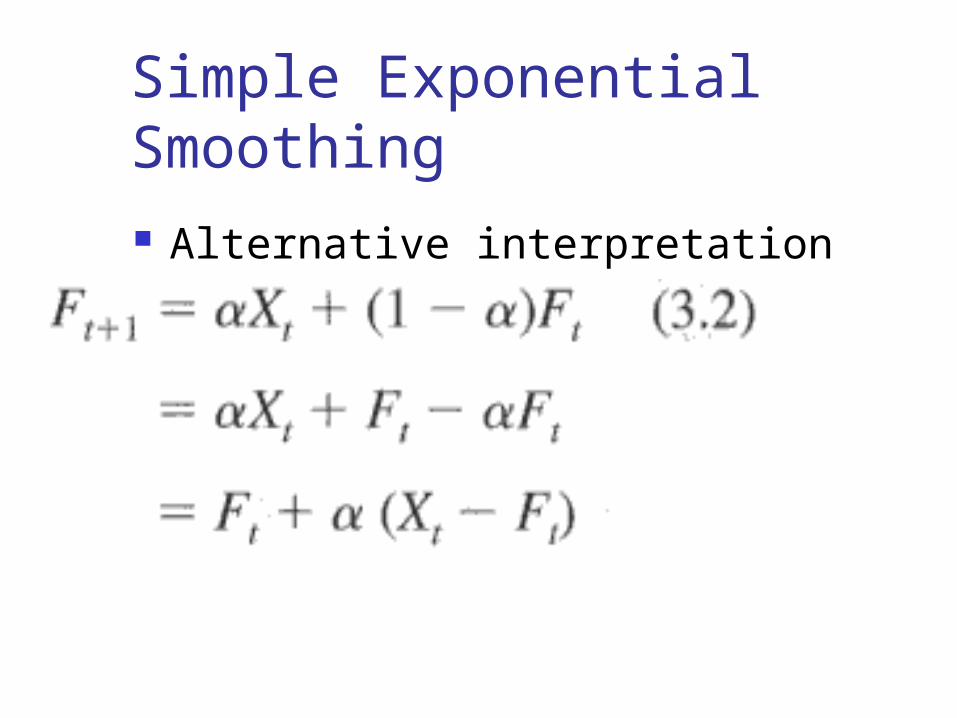
Simple Exponential Smoothing Alternative interpretation
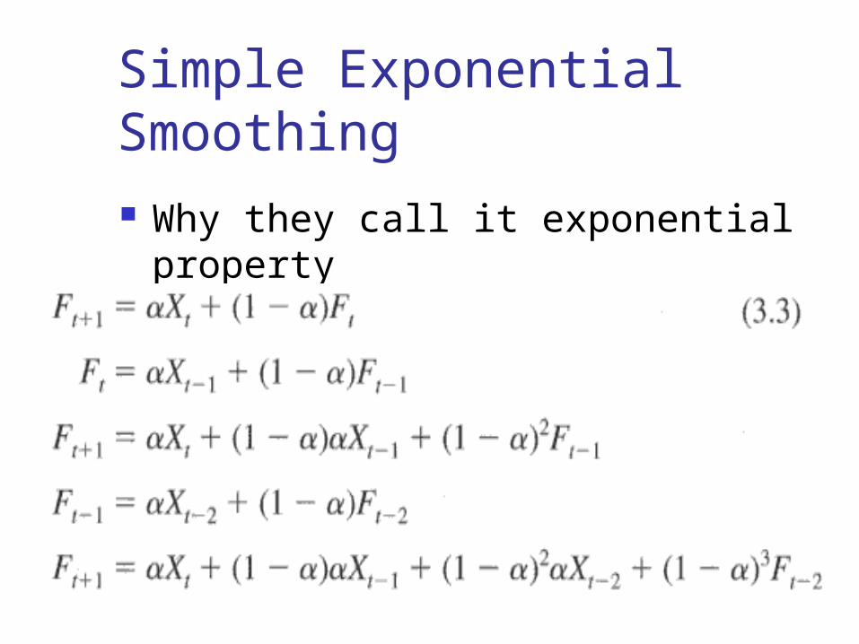
Simple Exponential Smoothing Why they call it exponential
property

Simple Exponential Smoothing Advantages
Simpler than other forms Requires limited data
Disdvantages Lags behind actual data No trend or seasonality

Holt's Exponential Smoothing(Double Holt in ForecastXTM)

ForecastXTM Conventions forSmoothing Constants
Alpha () =the simple smoothing constant
Gamma () =the trend smoothing constant
Beta () =the seasonality smoothing constant
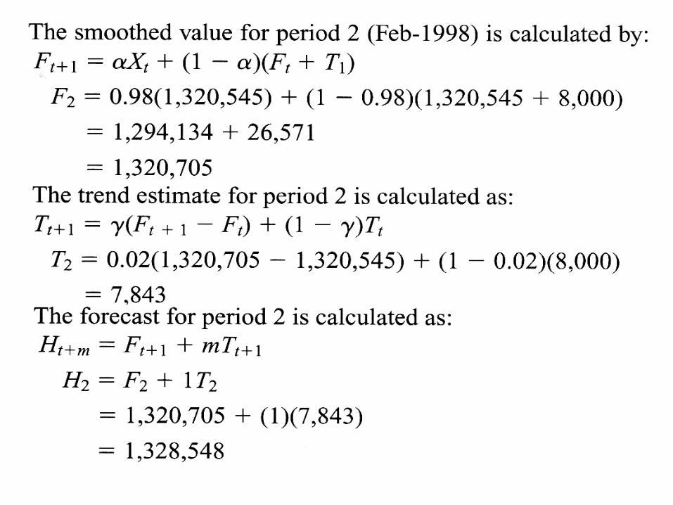
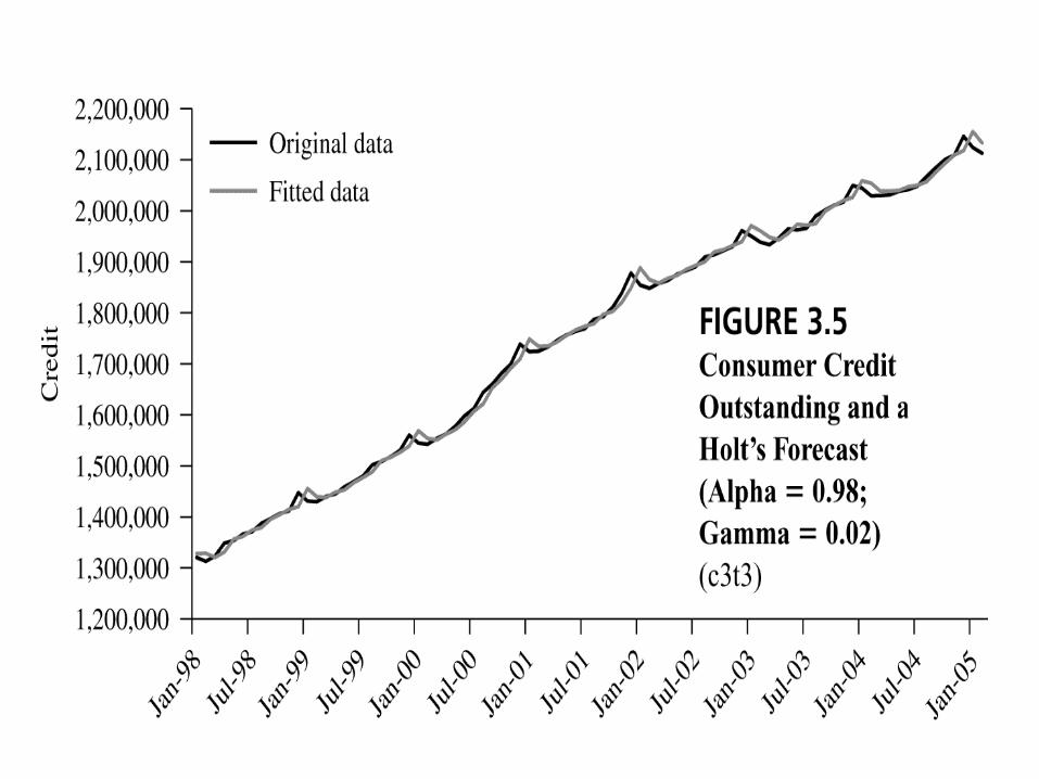
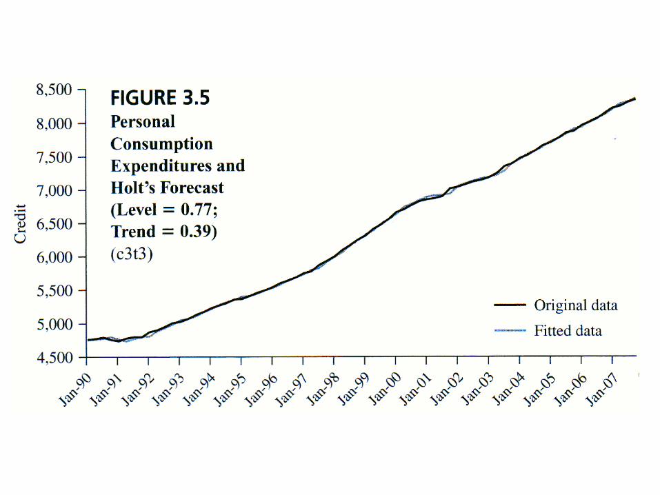

Holt's Exponential Smoothing ForecastX will pick the smoothing
constants to minimize RMSE Some trend, but no seasonality Call it linear trend smoothing
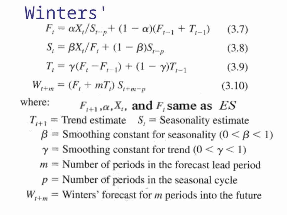
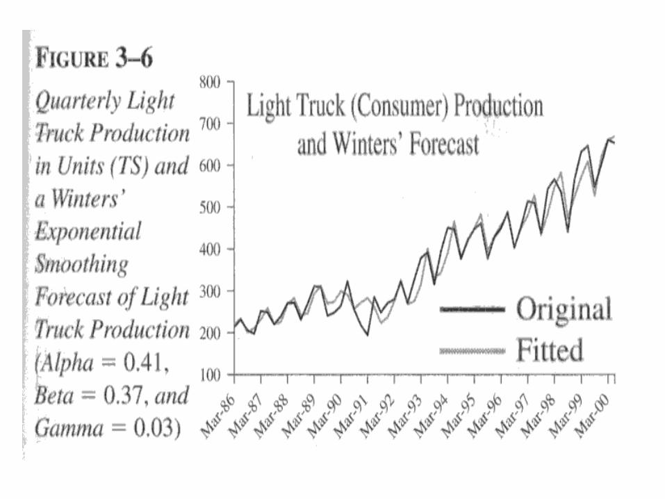
Winters'

Adaptive-Response-Rate Single Exponential Smoothing
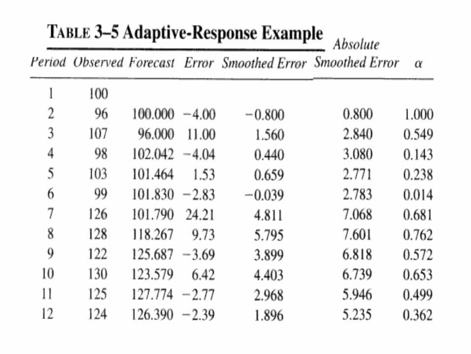

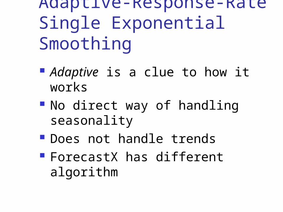
Adaptive-Response-Rate Single Exponential Smoothing Adaptive is a clue to how it works No direct way of handling
seasonality Does not handle trends ForecastX has different algorithm
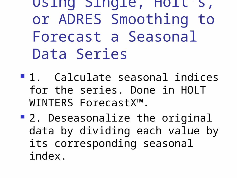
Using Single, Holt's, or ADRES Smoothing to Forecast a Seasonal Data Series
1. Calculate seasonal indices for the series. Done in HOLT WINTERS ForecastX™.
2. Deseasonalize the original data by dividing each value by its corresponding seasonal index.
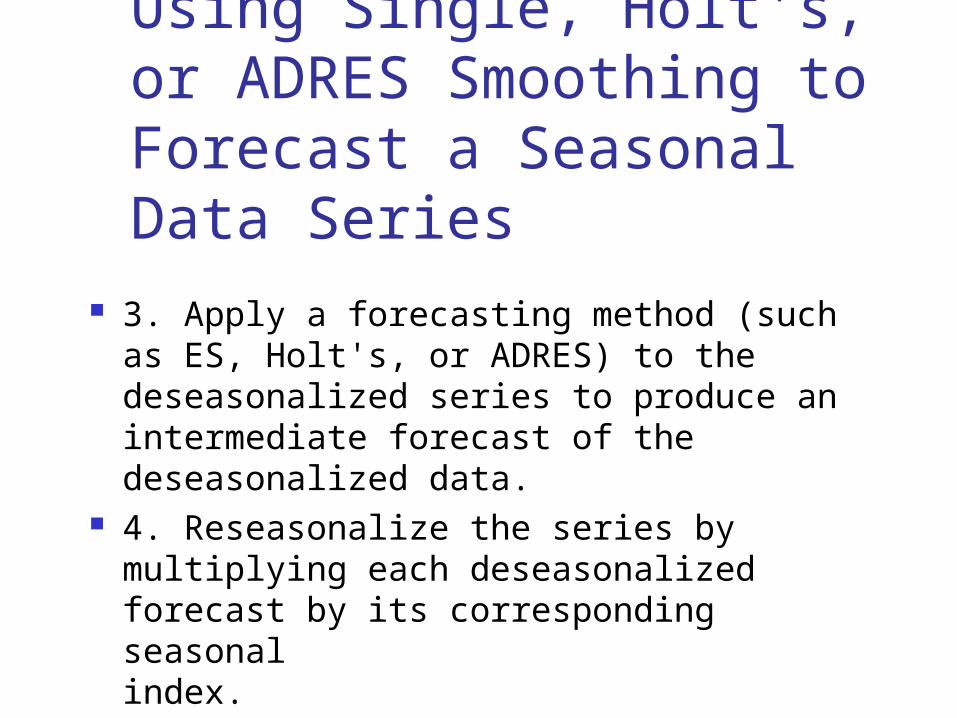
Using Single, Holt's, or ADRES Smoothing to Forecast a Seasonal Data Series
3. Apply a forecasting method (such as ES, Holt's, or ADRES) to the deseasonalized series to produce an intermediate forecast of the deseasonalized data.
4. Reseasonalize the series by multiplying each deseasonalized forecast by its corresponding seasonal index.

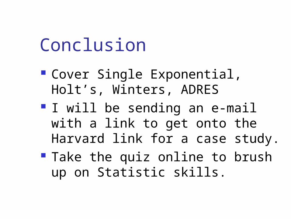
Conclusion Cover Single Exponential, Holt’s,
Winters, ADRES I will be sending an e-mail with a
link to get onto the Harvard link for a case study.
Take the quiz online to brush up on Statistic skills.


