11-0663_fig 04
Oaklan
d B
ay G oldsborough Cr e ek
Johns C ree k
Hood Canal
Skokomish Riv er
106
!(3
101
101
101
123°05'10'123°15'
47°20'
47°15'
Prepared in cooperation with the Washington State Department of Ecology
Hydrogeologic Framework of the Johns Creek Subbasin and Vicinity, Mason County, Washington
U.S. Department of the InteriorU.S. Geological Survey
Scientific Investigations Report 2011–5168

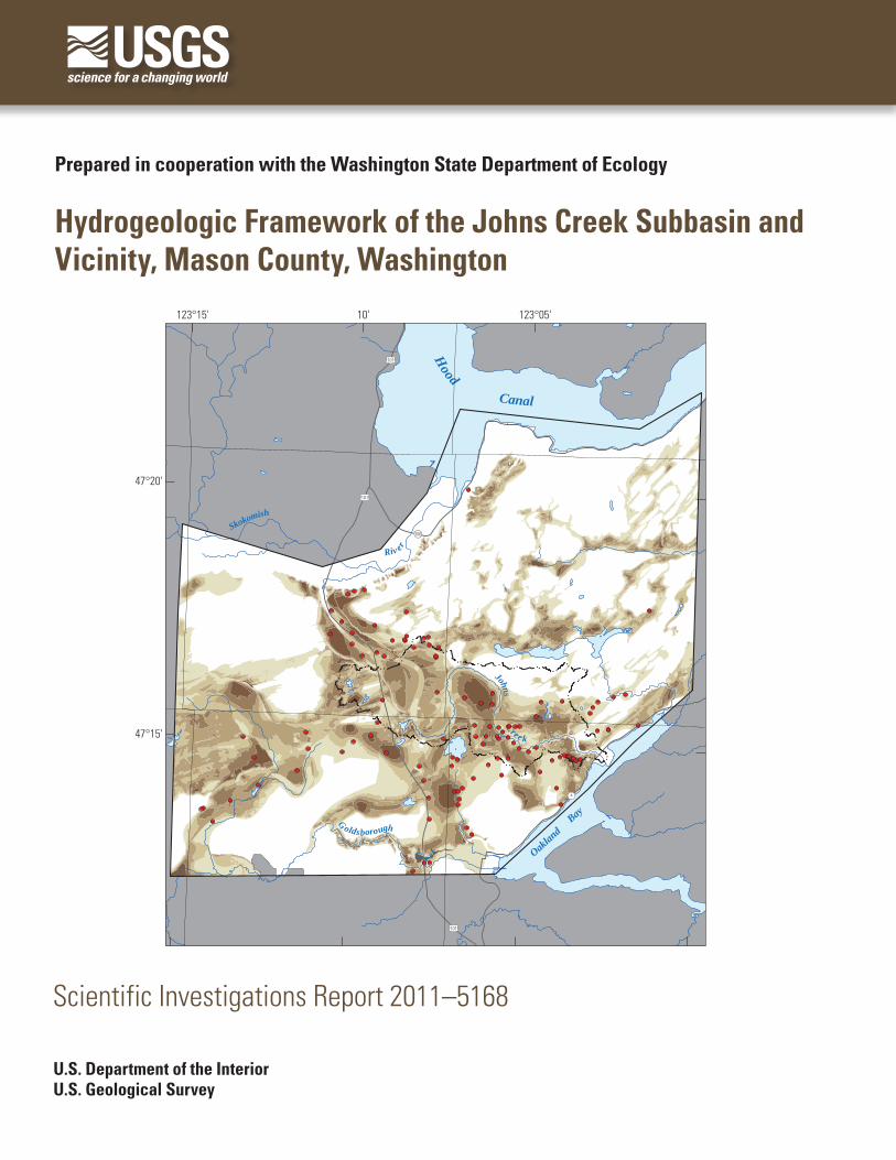
Cover: Representation of an aquifer extent and thickness map, Johns Creek subbasin and vicinity, Mason County, Washington
Hydrogeologic Framework of the Johns Creek Subbasin and Vicinity, Mason County, Washington
By Wendy B. Welch and Mark E. Savoca
Prepared in cooperation with the Washington State Department of Ecology
Scientific Investigations Report 2011–5168
U.S. Department of the InteriorU.S. Geological Survey

U.S. Department of the InteriorKEN SALAZAR, Secretary
U.S. Geological SurveyMarcia K. McNutt, Director
U.S. Geological Survey, Reston, Virginia: 2011
For more information on the USGS—the Federal source for science about the Earth, its natural and living resources, natural hazards, and the environment, visit http://www.usgs.gov or call 1–888–ASK–USGS.
For an overview of USGS information products, including maps, imagery, and publications, visit http://www.usgs.gov/pubprod
To order this and other USGS information products, visit http://store.usgs.gov
Any use of trade, product, or firm names is for descriptive purposes only and does not imply endorsement by the U.S. Government.
Although this report is in the public domain, permission must be secured from the individual copyright owners to reproduce any copyrighted materials contained within this report.
Suggested citation:Welch, W.B., and Savoca, M.E., 2011, Hydrogeologic framework of the Johns Creek subbasin and vicinity, Mason County, Washington: U.S. Geological Survey Scientific Investigations Report 2011–5168, 16 p., 1 pl.
iii
Contents
Abstract ...........................................................................................................................................................1Introduction.....................................................................................................................................................1
Purpose and Scope ..............................................................................................................................1Description of Study Area ...................................................................................................................1Geologic Setting ...................................................................................................................................3
Methods of Investigation .............................................................................................................................3Hydrogeologic Framework ...........................................................................................................................7Summary........................................................................................................................................................16Acknowledgments .......................................................................................................................................16References Cited..........................................................................................................................................16
Plate Plate 1. Map and hydrogeologic sections showing surficial hydrogeology, hydrogeologic
units, and locations of wells, Johns Creek subbasin and vicinity, Mason County, Washington.
Figures Figure 1. Map showing location of Johns Creek subbasin and vicinity, Mason County,
Washington ……………………………………………………………………… 2 Figure 2. Graphs showing residuals between hydrogeologic unit correlation altitudes
and altitudes of interpolated digital hydrogeologic surfaces for Johns Creek subbasin, Mason County, Washington …………………………………………… 6
Figure 3. Map showing extent and thickness of alluvial aquifer (AA) in Johns Creek subbasin and vicinity, Mason County, Washington ……………………………… 8
Figure 4. Map showing extent and thickness of upper aquifer (UA) in Johns Creek subbasin and vicinity, Mason County, Washington ……………………………… 9
Figure 5. Map showing extent and thickness of upper confining unit (UC) in Johns Creek subbasin and vicinity, Mason County, Washington ………………………… 11
Figure 6. Map showing extent and thickness of middle aquifer (MA) in Johns Creek subbasin and vicinity, Mason County, Washington ……………………………… 12
Figure 7. Map showing extent and thickness of lower confining unit (LC) in Johns Creek subbasin and vicinity, Mason County, Washington ………………………… 13
Figure 8. Map showing extent and thickness of lower aquifer (LA) in Johns Creek subbasin and vicinity, Mason County, Washington ……………………………… 14
Figure 9. Map showing extent and thickness of undifferentiated deposits (UD) in Johns Creek subbasin and vicinity, Mason County, Washington ………………… 15
Tables Table 1. Hydrogeologic units defined in this study and correlation with geologic and
hydrogeologic units defined by previous investigations ………………………… 4 Table 2. Statistics for the interpolated digital hydrogeologic surfaces …………………… 5
iv
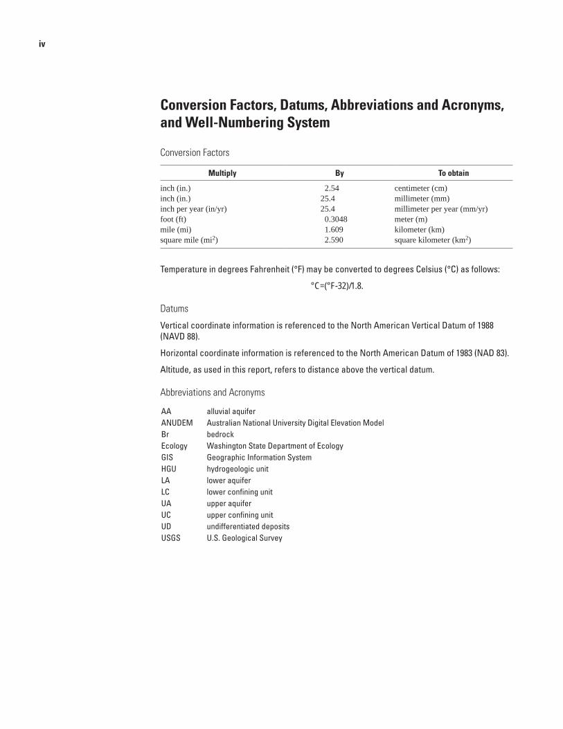
Conversion Factors, Datums, Abbreviations and Acronyms, and Well-Numbering System
Conversion Factors
Multiply By To obtain
inch (in.) 2.54 centimeter (cm)inch (in.) 25.4 millimeter (mm)inch per year (in/yr) 25.4 millimeter per year (mm/yr)foot (ft) 0.3048 meter (m)mile (mi) 1.609 kilometer (km)square mile (mi2) 2.590 square kilometer (km2)
Temperature in degrees Fahrenheit (°F) may be converted to degrees Celsius (°C) as follows:
°C=(°F-32)/1.8.
Datums
Vertical coordinate information is referenced to the North American Vertical Datum of 1988 (NAVD 88).
Horizontal coordinate information is referenced to the North American Datum of 1983 (NAD 83).
Altitude, as used in this report, refers to distance above the vertical datum.
Abbreviations and Acronyms
AA alluvial aquiferANUDEM Australian National University Digital Elevation ModelBr bedrockEcology Washington State Department of EcologyGIS Geographic Information SystemHGU hydrogeologic unitLA lower aquifer LC lower confining unitUA upper aquiferUC upper confining unitUD undifferentiated depositsUSGS U.S. Geological Survey
v
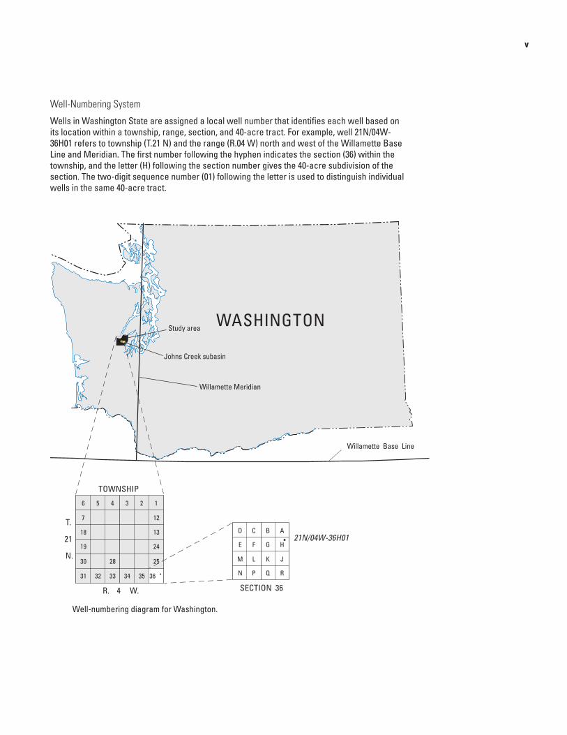
Well-Numbering System
Wells in Washington State are assigned a local well number that identifies each well based on its location within a township, range, section, and 40-acre tract. For example, well 21N/04W-36H01 refers to township (T.21 N) and the range (R.04 W) north and west of the Willamette Base Line and Meridian. The first number following the hyphen indicates the section (36) within the township, and the letter (H) following the section number gives the 40-acre subdivision of the section. The two-digit sequence number (01) following the letter is used to distinguish individual wells in the same 40-acre tract.
Well-numbering diagram for Washington.
watac0663_fig. well nunbering
Willamette Meridian
Willamette Base Line
WASHINGTONStudy area
Johns Creek subasin
SECTION 36
TOWNSHIP
21N/04W-36H01ABCD
E F G H
JKLM
N P Q R
R. 4 W.
T.
21
N.
123456
7 12
1318
19 24
252830
31 32 33 34 35 36

vi
This page intentionally left blank.
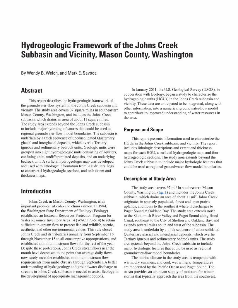
Hydrogeologic Framework of the Johns Creek Subbasin and Vicinity, Mason County, Washington
By Wendy B. Welch, and Mark E. Savoca
AbstractThis report describes the hydrogeologic framework of
the groundwater-flow system in the Johns Creek subbasin and vicinity. The study area covers 97 square miles in southeastern Mason County, Washington, and includes the Johns Creek subbasin, which drains an area of about 11 square miles. The study area extends beyond the Johns Creek subbasin to include major hydrologic features that could be used as regional groundwater-flow model boundaries. The subbasin is underlain by a thick sequence of unconsolidated Quaternary glacial and interglacial deposits, which overlie Tertiary igneous and sedimentary bedrock units. Geologic units were grouped into eight hydrogeologic units consisting of aquifers, confining units, undifferentiated deposits, and an underlying bedrock unit. A surficial hydrogeologic map was developed and used with lithologic information from 200 drillers’ logs to construct 4 hydrogeologic sections, and unit extent and thickness maps.
IntroductionJohns Creek in Mason County, Washington, is an
important producer of coho and chum salmon. In 1984, the Washington State Department of Ecology (Ecology) established an Instream Resources Protection Program for Water Resource Inventory Area 14 (WAC 173-514) to retain sufficient in-stream flow to protect fish and wildlife, scenic, aesthetic, and other environmental values. This rule closed Johns Creek and its tributaries annually from September 16 through November 15 to all consumptive appropriations, and established minimum instream flows for the rest of the year. Despite these protections, Johns Creek streamflows near the mouth have decreased to the point that average daily flows now rarely meet the established minimum instream flow requirements from mid-February through September. A better understanding of hydrogeology and groundwater discharge to streams in Johns Creek subbasin is needed to assist Ecology in the development of appropriate management options.
In January 2011, the U.S. Geological Survey (USGS), in cooperation with Ecology, began a study to characterize the hydrogeologic units (HGUs) in the Johns Creek subbasin and vicinity. These data are anticipated to be integrated, along with other information, into a numerical groundwater-flow model to contribute to improved understanding of water resources in the area.
Purpose and Scope
This report presents information used to characterize the HGUs in the Johns Creek subbasin, and vicinity. The report includes lithologic descriptions and extent and thickness maps for each HGU, a surficial hydrogeologic map, and four hydrogeologic sections. The study area extends beyond the Johns Creek subbasin to include major hydrologic features that could be used as regional groundwater-flow model boundaries.
Description of Study Area
The study area covers 97 mi2 in southeastern Mason County, Washington, (fig. 1) and includes the Johns Creek subbasin, which drains an area of about 11 mi2. Johns Creek originates in sparsely populated, forest and open prairie uplands, and flows to the southeast where it discharges to Puget Sound at Oakland Bay. The study area extends north to the Skokomish River Valley and Puget Sound along Hood Canal, southeast to the City of Shelton and Oakland Bay, and extends several miles south and west of the subbasin. The study area is underlain by a thick sequence of unconsolidated Quaternary glacial and interglacial deposits, which overlie Tertiary igneous and sedimentary bedrock units. The study area extends beyond the Johns Creek subbasin to include major hydrologic features that could be used as regional groundwater-flow model boundaries.
The marine climate in the study area is temperate with warm, dry summers, and cool, wet winters. Temperatures are moderated by the Pacific Ocean and Puget Sound. The ocean provides an abundant supply of moisture for winter storms that typically approach the area from the southwest.

2 Hydrogeologic Framework of the Johns Creek Subbasin and Vicinity, Mason County, Washington
11-0663_fig 01
EXPLANATIONStudy area boundary
Johns Creek subbasin
Base from U.S. Geological Survey digital data, 1:120,000Lambert Conformal Conic projection: State Plane Washington SouthNorth American Datum 1983
SheltonOak
land
Bay
CranberryLake
Lake Limerick
Island Lake
Goose Lake
Johns Lake
McT
agge
rt C
reek
North
F
ork
S
koko
mish R
iver
Purd
y Cr eek
Weaver Creek
Winter Creek
G oldsborough Cr e ek
North F ork
Sou
th
Fo
rk
Coffee Cree
k
Johns C ree k
Shelton Cr eek
Schumacher Creek
Cran berry Creek
Hammersley Inlet
Hood Canal
Skokomish Riv er
Mill Creek
106
!(3
101
101
101
123°05'10'123°15'
47°20'
47°15'
T22N
T21N
T20N
R. 04 W. R. 04 W.R. 03 W. R. 03 W. 0 1 2 3 4
0 4321 KILOMETERS
MILES
WASHINGTON
Figure location
PAC
IFIC
OCE
AN
Puge
t Sou
ndPu
get S
ound
Figure 1. Location of Johns Creek subbasin and vicinity, Mason County, Washington.

Methods of Investigation 3
The annual average precipitation (1971–2000) at Shelton (fig. 1) is 65.7 in/yr (National Oceanic and Atmospheric Administration, 2007). The distribution of precipitation varies throughout the year. Summers (June–August) typically are dry with an average total precipitation at Shelton of 4.0 in. Winters (December–February) are wetter than summers with an average total precipitation of 29.4 in. The average monthly temperature (1971–2000) at Shelton ranges from about 39 °F in December to about 65 °F in August (National Oceanic and Atmospheric Administration, 2007).
Geologic Setting
The summary of major geologic events in the study area is based on the work of Easterbrook (1969), Molenaar and Noble (1970), Schasse and others (2003), and Polenz and others (2010). Tectonic forces related to subduction of oceanic crust beneath the western coast of North America resulted in uplift and accretion of Eocene igneous and sedimentary rocks along the continental margin. These deformed rocks form the bedrock beneath the study area in southeastern Mason County. The Puget Lobe of the Cordilleran ice sheet advanced into the study area several times during the Pleistocene Epoch. The most recent period of glaciation, the Vashon Stade of Fraser glaciation, began about 17,000 years ago when the continental ice sheet in Canada expanded, and the Puget Lobe advanced southward, eventually covering the entire Puget Sound basin before halting and retreating. Unconsolidated deposits of glacial and interglacial origin are present throughout the study area and typically range in thickness from 600 to more than 1,000 ft. A typical glacial sequence progresses from advance outwash, to till, to recessional outwash. Fluvial, lacustrine, bog, and marsh depositional environments were common during interglacial periods.
Methods of Investigation The HGUs in the Johns Creek subbasin and vicinity
were defined using previously published geologic maps, well records with drillers’ logs available from Ecology, and previous investigations by Molenaar and Noble (1970) and Northwest Land and Water, Inc. (2005). The surficial hydrogeologic map for the study area (pl. 1; scale 1:40,000) was produced by merging available digital surficial geologic maps (Logan 2003; scale 1:100,000; Schasse and others, 2003, scale 1:24,000; Polenz and others, 2010, scale 1:24,000.)
Thirty-six geologic units delineated on these source maps were grouped into 8 HGUs based on similarities in lithology (grain size and sorting), hydrologic characteristics, and relative stratigraphic position (table 1).
Well records that document the drilling (drillers’ log description of borehole lithology) and construction were compiled from the Ecology database to identify potential wells for use in this study. Candidate wells were selected based on their spatial distribution, depth of the well, and availability of a complete well record with drillers’ log. The goal was to obtain an even distribution of wells throughout the study area; however, this was not possible for the entire study area because of a lack of wells in less populated areas. Because there was no field inventory of wells conducted for this study, locations of wells were obtained from records of previous investigations, well addresses from drillers’ logs, and locations in quarter-quarter sections recorded in the Ecology database.
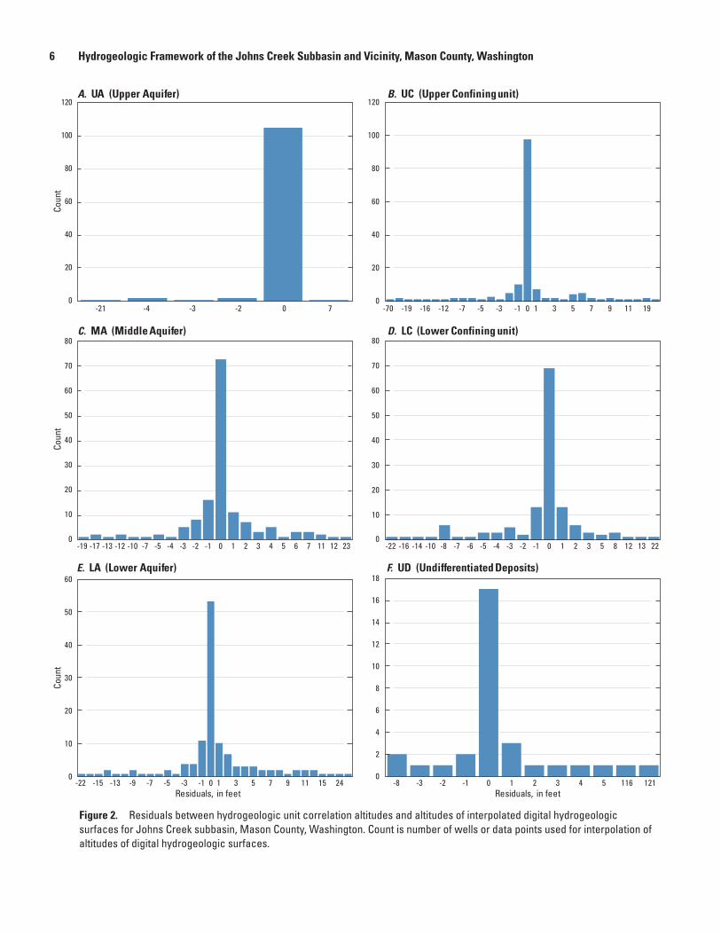
The surficial hydrogeologic map and lithologic data from 200 drillers’ logs were used to construct several hydrogeologic sections using A-Prime Software’s CrossView™ for ArcGIS® to identify and correlate the HGUs in the subsurface. Four representative hydrogeologic sections are shown in plate 1. HGUs were assigned to the various lithologic layers depicted in each well log based on lithology (grain size and sorting), hydrologic characteristics (aquifer or confining unit), and relative stratigraphic position. HGU assignments were used to delineate the extent of each unit throughout the study area. The altitude of the top surface of a unit was interpolated in a GIS at a 50 ft interpolation grid cell size, using a method based on the Australian National University Digital Elevation Model (ANUDEM) procedure developed by Hutchinson (1989). HGU top surfaces were constrained to a LiDAR-derived land surface digital elevation model (DEM) at locations where the units cropped out. If part of the top surface of a unit was interpolated above the top of an overlying unit then minimum thickness values for the overlying unit were used in the calculations to adjust the altitude of the top of the underlying unit where needed. Unit thickness maps were created by using the GIS to calculate the difference between the top of a unit and the interpolated top of the underlying unit(s). Residuals were calculated as the difference between the unit surface altitudes assigned for a specific well log and unit altitudes of the interpolated digital hydrogeologic surfaces at the location of the well. Statistics on the residuals were determined for each HGU, excluding the alluvial aquifer (AA), to provide a quantitative comparison between the specific well log data and the interpolated surfaces for the entire study area (table 2; fig 2). Residuals commonly were within ±1 ft for all HGUs.

4 Hydrogeologic Framework of the Johns Creek Subbasin and Vicinity, Mason County, WashingtonTa
ble
1.
Hydr
ogeo
logi
c un
its d
efin
ed in
this
stu
dy a
nd c
orre
latio
n w
ith g
eolo
gic
and
hydr
ogeo
logi
c un
its d
efin
ed b
y pr
evio
us in
vest
igat
ions
.
Peri
od
Epoc
hH
ydro
geol
ogic
uni
ts
defin
ed in
this
stu
dyLi
thol
ogy
Geo
logi
c un
its
in L
ogan
(2
003)
Geo
logi
c un
its in
Sc
hass
e an
d ot
hers
(200
3);
Pole
nz a
nd o
ther
s (2
010)
Hyd
roge
olog
ic u
nits
in
Nor
thw
est L
and
and
Wat
er (2
005)
Quaternary
Hol
ocen
e A
A –
Allu
vial
Aqu
ifer
rece
nt a
lluvi
al d
epos
itsG
rave
l, sa
nd, a
nd si
lt; c
lay
and
peat
Qa
Qa,
1 Qp,
Qf,
Qa(
m),
1 Qaf
, 1 Q
mw,
1 Qls
, Qm
, Qoa
, Qb,
af
, ml
Not
del
inea
ted
Pleistocene
UA
– U
pper
Aqu
ifer
rece
ssio
nal o
utw
ash
depo
sits
Sand
and
gra
vel;
lens
es o
f cla
y, si
lt,
and
fine
sand
Qgo
, Qap
o, Q
gdQ
gd,
Qgi
c, Q
gog,
Qgo
, Qgo
s, 1 Q
gik,
Qge
, 1 Qm
w, Q
gol,
1 Qgo
f, 1 Q
af, 1 Q
pU
nit A
UC
– U
pper
Con
finin
g un
it
glac
ial t
ill d
epos
its
Uns
orte
d an
d co
mpa
cted
cla
y, si
lt, sa
nd,
and
grav
el; l
ense
s of s
and
and
grav
elQ
gtQ
gt, Q
gta,
1 Qp,
Qgo
l, Q
ml
Uni
ts B
and
C
MA
– M
iddl
e Aqu
ifer
adva
nce
outw
ash
depo
sits
Sand
, gra
vel,
and
silt;
occ
asio
nal
lens
es o
f cla
y Q
gaQ
ga, Q
po, Q
pg(o
), 1 Q
gik
1 Qgo
f, 1 Q
mw,
1 Qls
, Qap
dU
nit D
LC –
Low
er C
onfin
ing
unit
glac
iola
cust
rine
and
inte
rgla
cial
se
dim
ents
Cla
y an
d si
lt; so
me
till;
occa
sion
al
peat
and
woo
dQ
c(k)
Qpu
(op)
, Qpf
, 1 Qgi
k, 1 Q
lsU
nit E
LA –
Low
er A
quife
r ou
twas
h, ti
ll, a
nd g
laci
olac
ustri
ne
depo
sits
Sand
and
gra
vel,
silt
and
clay
; som
e til
l
Qgp
Qpg
o, Q
pg, Q
pd, Q
pt
Uni
t FU
D –
Und
iffer
entia
ted
Dep
osits
un
diffe
rent
iate
d gl
acia
l and
in
terg
laci
al se
dim
ents
Alte
rnat
ing
laye
rs o
f cla
y an
d si
lt,
sand
and
gra
vel
2 Qu
Terti
ary
Eoce
neB
r – B
edro
ck
igne
ous a
nd se
dim
enta
ry ro
cks
Volc
anic
and
sedi
men
tary
rock
Ev(c
)2 E
v(c)
Bed
rock
1 Thi
n (le
ss th
an 1
0 fe
et) a
nd (o
r) d
isco
ntin
uous
geo
logi
c un
its (P
olen
z an
d ot
hers
, 201
0) in
ass
ocia
tion
with
aqu
ifer a
nd c
onfin
ing
hydr
ogeo
logi
c un
its a
t lan
d su
rfac
e.
2 Geo
logi
c un
its d
elin
eate
d on
ly in
Sch
asse
and
oth
ers (
2003
); no
equ
ival
ent g
eolo
gic
units
del
inea
ted
in P
olen
z an
d ot
hers
(201
0).
Methods of Investigation 5
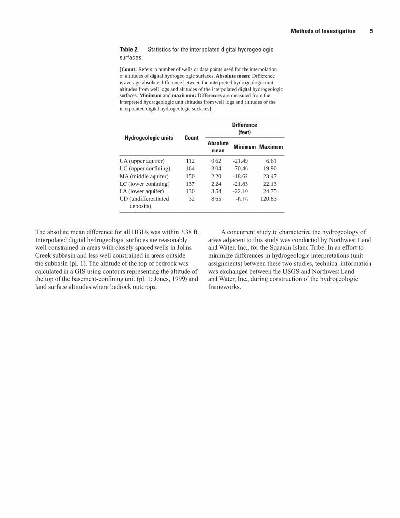
Table 2. Statistics for the interpolated digital hydrogeologic surfaces.
[Count: Refers to number of wells or data points used for the interpolation of altitudes of digital hydrogeologic surfaces. Absolute mean: Difference is average absolute difference between the interpreted hydrogeologic unit altitudes from well logs and altitudes of the interpolated digital hydrogeologic surfaces. Minimum and maximum: Differences are measured from the interpreted hydrogeologic unit altitudes from well logs and altitudes of the interpolated digital hydrogeologic surfaces]
Hydrogeologic units Count
Difference (feet)
Absolute mean
Minimum Maximum
UA (upper aquifer) 112 0.62 -21.49 6.61UC (upper confining) 164 3.04 -70.46 19.90MA (middle aquifer) 150 2.20 -18.62 23.47LC (lower confining) 137 2.24 -21.83 22.13LA (lower aquifer) 130 3.54 -22.10 24.75UD (undifferentiated
deposits)32 8.65 -8.16 120.83
The absolute mean difference for all HGUs was within 3.38 ft. Interpolated digital hydrogeologic surfaces are reasonably well constrained in areas with closely spaced wells in Johns Creek subbasin and less well constrained in areas outside the subbasin (pl. 1). The altitude of the top of bedrock was calculated in a GIS using contours representing the altitude of the top of the basement-confining unit (pl. 1; Jones, 1999) and land surface altitudes where bedrock outcrops.
A concurrent study to characterize the hydrogeology of areas adjacent to this study was conducted by Northwest Land and Water, Inc., for the Squaxin Island Tribe. In an effort to minimize differences in hydrogeologic interpretations (unit assignments) between these two studies, technical information was exchanged between the USGS and Northwest Land and Water, Inc., during construction of the hydrogeologic frameworks.
6 Hydrogeologic Framework of the Johns Creek Subbasin and Vicinity, Mason County, Washington
11-0663_fig 02
0
20
40
60
80
100
120
0
20
40
60
80
100
120
0
10
20
30
40
50
60
70
80
0
10
20
30
40
50
60
70
80
0
10
20
30
40
50
60
0
2
4
6
8
10
12
14
16
18
-21 -4 -3 -2 0 7
A. UA (Upper Aquifer) B. UC (Upper Confining unit)
C. MA (Middle Aquifer) D. LC (Lower Confining unit)
E. LA (Lower Aquifer) F. UD (Undifferentiated Deposits)
-70 -19 -16 -12 -7 -5 -3 -1 10 3 5 7 9 11 19
-19 -17 -13 -12 -10 -7 -5 -4 -3 -2 -1 0 1 2 3 4 5 6 7 11 12 23 -22 -16 -14 -10 -8 -7 -6 -5 -4 -3 -2 -1 0 1 2 3 5 8 12 13 22
-22 -15 -13 -9 -7 -5 -3 -1 10 3 5 7 9 11 15 24Residuals, in feet
Coun
tCo
unt
Coun
t
Residuals, in feet-8 -3 -2 -1 0 1 2 3 4 5 116 121
Figure 2. Residuals between hydrogeologic unit correlation altitudes and altitudes of interpolated digital hydrogeologic surfaces for Johns Creek subbasin, Mason County, Washington. Count is number of wells or data points used for interpolation of altitudes of digital hydrogeologic surfaces.
Hydrogeologic Framework 7
Hydrogeologic FrameworkThe hydrogeologic framework defines the physical,
lithologic, and hydrologic characteristics of the HGUs that compose the groundwater system in the study area. An understanding of these characteristics is important in determining the occurrence, movement, and availability of groundwater in aquifers within Johns Creek subbasin, and the exchange of water between the aquifers and creeks.
Geologic units were grouped into HGUs, consisting of aquifers and confining units (table 1) based on similarities in lithology (grain size and sorting), hydrologic characteristics, and relative stratigraphic position. The HGUs defined in this study (table 1) are based on units previously defined by Northwest Land and Water, Inc. (2005) in the study area. Differences between units defined in this study and those previously defined by Northwest Land and Water, Inc. (2005) include the: (1) addition of an alluvial aquifer unit, (2) combination of the B and C confining units into an upper confining unit (UC), and (3) division of unit F into a lower aquifer unit (LC) and undifferentiated deposits (UD).
An aquifer is saturated geologic material that is sufficiently permeable to yield water in significant quantities to a well or spring, whereas a confining unit has low permeability that restricts the movement of groundwater and limits the usefulness of the unit as a water source. Unconfined and confined conditions are present in aquifers in Johns Creek subbasin and affect the movement and storage of groundwater. Unconfined conditions occur when the upper surface of the saturated zone (water table) is at atmospheric pressure and the water table is free to rise and decline, filling and draining pore space, respectively, in response to changes in groundwater recharge and discharge. Confined conditions occur when groundwater pressure exceeds atmospheric pressure due to the presence of a less permeable overlying unit that constrains the thickness of the saturated zone. Changes in fluid pressure or head under confined conditions in response to groundwater recharge and discharge are governed by the compressibilities of the fluid and the skeletal matrix of the unit and do not result in filling or draining pore space.
Glacial deposits are generally heterogeneous, and although a glacial aquifer may be composed primarily of sand or gravel, it may locally contain varying amounts of clay or silt. Similarly, a confining layer composed predominantly of silt or clay may contain local lenses of coarser-grained material. Aquifers in the study area consist primarily of recent alluvium and glacial outwash, but may include coarse-grained interglacial deposits. The confining units consist primarily of glacial till, glaciolacustrine deposits, and fine-grained interglacial deposits. Unconsolidated glacial and interglacial aquifer and confining units are underlain by low-permeability Tertiary bedrock units, described as the basement-confining unit in Jones (1999). Eight HGUs are recognized in the study area (table 1, pl. 1) and their lithologic and hydrologic characteristics are described below.
Alluvial Aquifer (AA) – The alluvial aquifer is present at land surface throughout the Skokomish River Valley, along parts of Johns Creek and other local creeks, and in discontinuous or isolated bodies in marsh areas and depressions in upland areas (pl. 1). The aquifer also is projected under Hood Canal at the mouth of the Skokomish River based on unit top altitudes and bathymetry (pl. 1). The aquifer consists of alluvial gravel, sand, and silt, with clay and peat deposits. The thickness of the alluvial aquifer ranges from 5 to 229 ft with an average thickness of 17 ft (fig. 3). Groundwater in this aquifer generally is unconfined; however, confined conditions may occur locally beneath clay deposits.
Upper Aquifer (UA) – The upper aquifer is present at land surface throughout much of central and western parts of the study area, in discontinuous or isolated bodies within depressions in upland areas, and beneath alluvial aquifer deposits along parts of Johns and Goldsborough Creeks (pl. 1). The upper aquifer primarily is composed of Vashon recessional outwash deposits of the Fraser Glaciation and consists of sand and gravel, with lenses of clay, silt, and fine sand deposited by large melt-water streams formed during the northward retreat of the Puget Lobe. The thickness of the upper aquifer ranges from 5 to 255 ft with an average thickness of 34 ft (fig. 4). Groundwater in this aquifer generally is unconfined; however, confined conditions may occur locally beneath clay deposits.

8 Hydrogeologic Framework of the Johns Creek Subbasin and Vicinity, Mason County, Washington
11-0663_fig 03
EXPLANATION
Study area boundary
Johns Creek subbasin 5 to 16
17 to 31
32 to 52
53 to 110
111 to 229
Bedrock outcrop
Well—Used to determine extent and thickness ofAlluvial Aquifer (AA)—See plate 1
Extent and thickness ofAlluvial Aquifer (AA), in feet
Base from U.S. Geological Survey digital data, 1:120,000Lambert Conformal Conic projection: State Plane Washington SouthNorth American Datum 1983
Oaklan
d B
ay G oldsborough Cr e ek
Johns C ree k
Hood Canal
Skokomish Riv er
106
!(3
101
101
101
123°05'10'123°15'
47°20'
47°15'
T22N
T21N
T20N
R. 04 W. R. 04 W.R. 03 W. R. 03 W. 0 1 2 3 4
0 4321 KILOMETERS
MILES
Figure 3. Extent and thickness of alluvial aquifer (AA) in Johns Creek subbasin and vicinity, Mason County, Washington.

Hydrogeologic Framework 9
11-0663_fig 04
EXPLANATION
Study area boundary
Johns Creek subbasin 5 to 20
21 to 36
37 to 52
53 to 72
73 to 255
Bedrock outcrop
Well—Used to determine extent and thickness of
Upper Aquifer (UA)—See plate 1
Extent and thickness ofUpper Aquifer (UA), in feet
Base from U.S. Geological Survey digital data, 1:120,000Lambert Conformal Conic projection: State Plane Washington SouthNorth American Datum 1983
Oaklan
d B
ay G oldsborough Cr e ek
Johns C ree k
Hood Canal
Skokomish Riv er
106
!(3
101
101
101
123°05'10'123°15'
47°20'
47°15'
T22N
T21N
T20N
R. 04 W. R. 04 W.R. 03 W. R. 03 W. 0 1 2 3 4
0 4321 KILOMETERS
MILES
Figure 4. Extent and thickness of upper aquifer (UA) in Johns Creek subbasin and vicinity, Mason County, Washington.

10 Hydrogeologic Framework of the Johns Creek Subbasin and Vicinity, Mason County, Washington
Upper Confining unit (UC) – The upper confining unit is present in the subsurface throughout most of the study area (fig. 5), with numerous surficial exposures in upland areas (pl. 1). This low-permeability unit primarily is composed of Vashon till and consists of unsorted and compacted clay, silt, sand, and gravel, with locally occurring lenses of sand and gravel capable of providing water for domestic use. The thickness of the upper confining unit ranges from 5 to 359 ft with an average thickness of 57 ft (fig. 5).
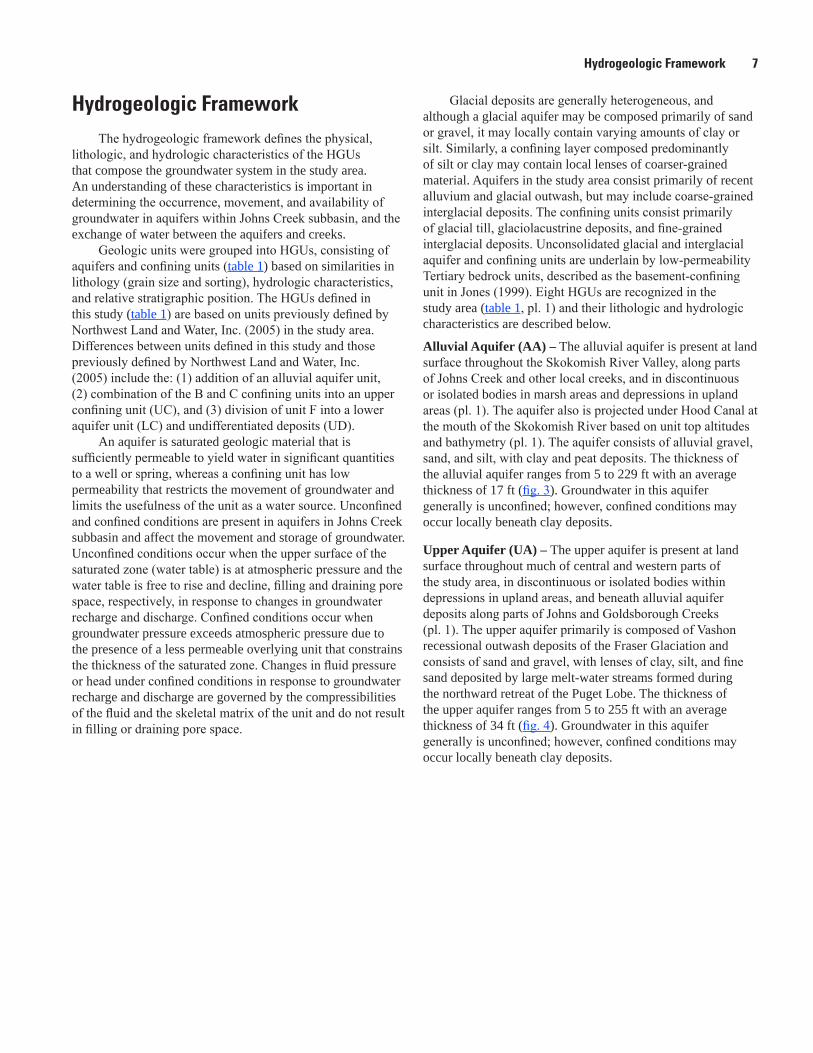
Middle Aquifer (MA) – The middle aquifer is present in the subsurface throughout most of the study area (fig. 6). Surficial exposures of the middle aquifer are limited to areas along the bluffs of the Skokomish River Valley and Puget Sound, bluffs along Goldsborough Creek near Oakland Bay, and isolated bodies within depressions in upland areas (pl. 1). The middle aquifer primarily is composed of Vashon advance outwash and consists of sand, gravel, and silt, with occasional lenses of clay. The thickness of the middle aquifer averages about 62 ft, but varies spatially from a thin veneer to about 150 ft (fig. 6) In two areas with low data density, the thickness exceeds 200 ft. Groundwater in this aquifer generally is confined by the overlying upper confining unit; however, unconfined conditions may occur locally where the aquifer is not fully saturated or is exposed at the surface.
Lower Confining unit (LC) – The lower confining unit is present in the subsurface throughout most of the study area (fig. 7). Surficial exposures of the lower confining unit are limited to areas along the bluffs of the Skokomish River Valley and Puget Sound and along a deep incision of Goldsborough Creek west of Shelton (pl. 1). Exposures of the lower confining unit are projected beneath Oakland Bay based on unit top altitudes and bathymetry. This low-permeability unit is primarily composed of pre-Vashon glaciolacustrine and interglacial sediments and consists of clay and silt, with some till and occasional deposits of peat and wood. The average thickness of the lower confining unit is 106 ft but locally exceeds 350 ft in areas with low data density (fig. 7).
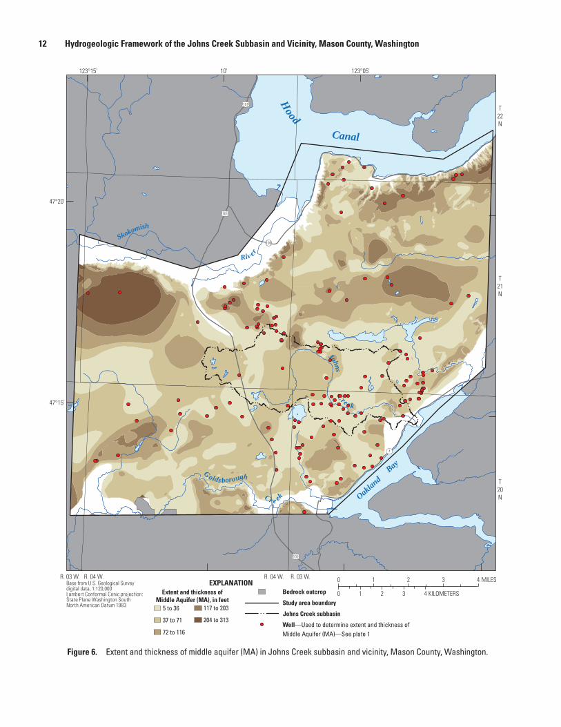
Lower Aquifer unit (LA) – The lower aquifer unit is present in the subsurface throughout most of the study area (fig. 8), and is not present at land surface except where it is projected beneath Hood Canal based on unit top altitudes and bathymetry (pl. 1). The aquifer is primarily composed of pre-Vashon outwash deposits and consists of sand and gravel, silt and clay, with some till deposits. The thickness of the lower aquifer typically ranges from 5 to 200 ft with an average thickness of 105 ft (fig. 8). Groundwater in this aquifer generally is confined by the overlying lower confining unit.
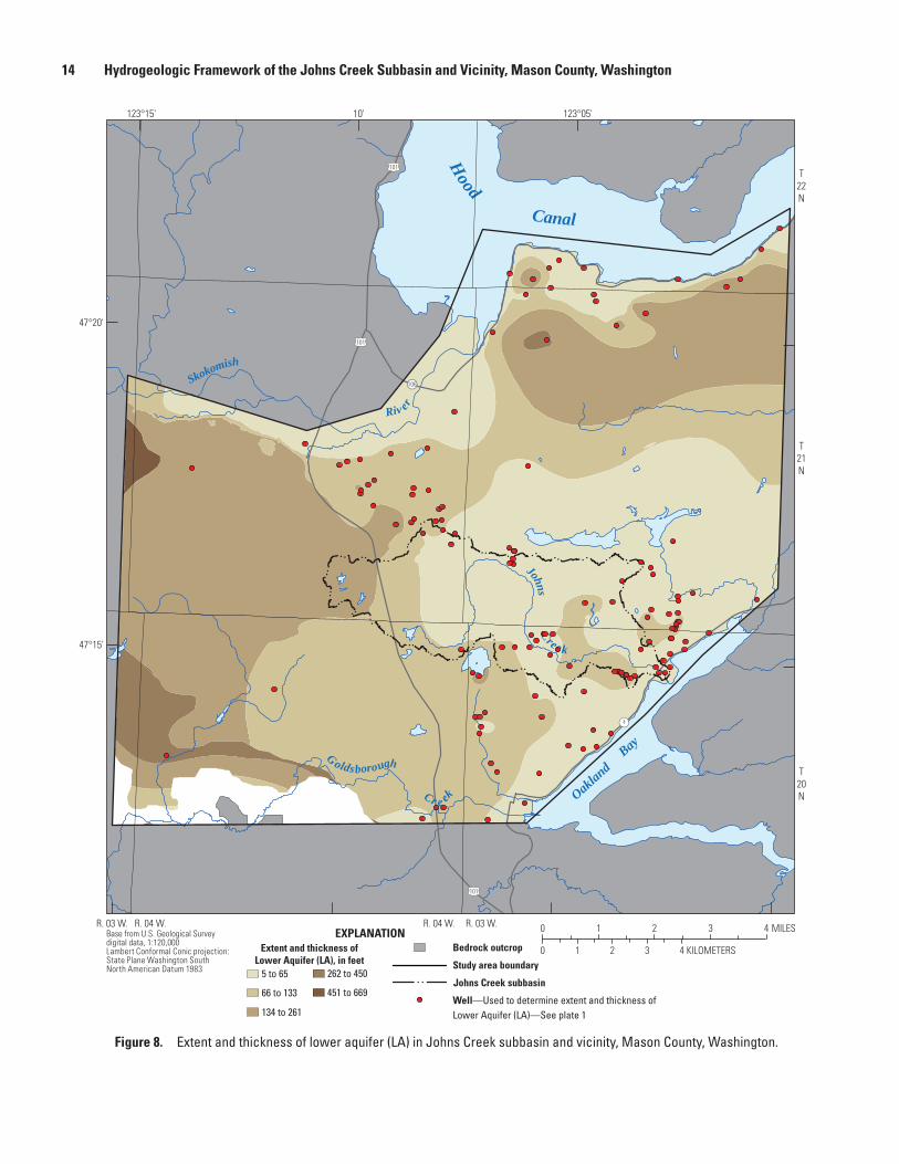
Undifferentiated Deposits (UD) – Undifferentiated deposits are present in the subsurface throughout most of the study area (fig. 9), and are not present at land surface except where it is projected beneath Hood Canal based on unit top elevations and bathymetry (pl. 1). Undifferentiated deposits are composed of pre-Vashon glacial and interglacial sediments and consist of alternating layers of clay and silt, and sand and gravel. The thickness of undifferentiated deposits was computed by subtracting the top of bedrock from the top of the undifferentiated unit (fig. 9). Groundwater in the undifferentiated deposits is likely confined by overlying layers of clay and silt.
Bedrock (Br) – Bedrock outcrops are limited to a few places along the southwestern margin of the study area (pl. 1). This low-permeability unit consists of Tertiary extrusive (basalt) and intrusive (diabase and gabbro) igneous and sedimentary (siltstone and sandstone) rocks.

Hydrogeologic Framework 11
11-0663_fig 05
5 to 30
31 to 56
57 to 83
84 to 115
116 to 359
Extent and thickness of UpperConfining unit (UC), in feet
EXPLANATION
Study area boundary
Johns Creek subbasin
Bedrock outcrop
Well—Used to determine extent and thickness ofUpper Confining unit (UC)—See plate 1
Base from U.S. Geological Survey digital data, 1:120,000Lambert Conformal Conic projection: State Plane Washington SouthNorth American Datum 1983
Oaklan
d B
ay G oldsborough Cr e ek
Johns C ree k
Hood Canal
Skokomish Riv er
106
!(3
101
101
101
123°05'10'123°15'
47°20'
47°15'
T22N
T21N
T20N
R. 04 W. R. 04 W.R. 03 W. R. 03 W. 0 1 2 3 4
0 4321 KILOMETERS
MILES
Figure 5. Extent and thickness of upper confining unit (UC) in Johns Creek subbasin and vicinity, Mason County, Washington.
12 Hydrogeologic Framework of the Johns Creek Subbasin and Vicinity, Mason County, Washington
11-0663_fig 06
5 to 36
37 to 71
72 to 116
117 to 203
204 to 313
Extent and thickness ofMiddle Aquifer (MA), in feet
EXPLANATION
Study area boundary
Johns Creek subbasin
Bedrock outcrop
Well—Used to determine extent and thickness ofMiddle Aquifer (MA)—See plate 1
Base from U.S. Geological Survey digital data, 1:120,000Lambert Conformal Conic projection: State Plane Washington SouthNorth American Datum 1983
Oaklan
d B
ay G oldsborough Cr e ek
Johns C ree k
Hood Canal
Skokomish Riv er106
!(3
101
101
101
123°05'10'123°15'
47°20'
47°15'
T22N
T21N
T20N
R. 04 W. R. 04 W.R. 03 W. R. 03 W. 0 1 2 3 4
0 4321 KILOMETERS
MILES
Figure 6. Extent and thickness of middle aquifer (MA) in Johns Creek subbasin and vicinity, Mason County, Washington.

Hydrogeologic Framework 13
11-0663_fig 07
5 to 63
64 to 139
140 to 226
227 to 378
379 to 675
Extent and thickness of LowerConfining unit (LC), in feet
EXPLANATION
Study area boundary
Johns Creek subbasin
Bedrock outcrop
Well—Used to determine extent and thickness ofLower Confining unit (LC)—See plate 1
Base from U.S. Geological Survey digital data, 1:120,000Lambert Conformal Conic projection: State Plane Washington SouthNorth American Datum 1983
Oaklan
d B
ay G oldsborough Cr e ek
Johns C ree k
Hood Canal
Skokomish Riv er
106
!(3
101
101
101
123°05'10'123°15'
47°20'
47°15'
T22N
T21N
T20N
R. 04 W. R. 04 W.R. 03 W. R. 03 W. 0 1 2 3 4
0 4321 KILOMETERS
MILES
Figure 7. Extent and thickness of lower confining unit (LC) in Johns Creek subbasin and vicinity, Mason County, Washington.
14 Hydrogeologic Framework of the Johns Creek Subbasin and Vicinity, Mason County, Washington
11-0663_fig 08
5 to 65
66 to 133
134 to 261
262 to 450
451 to 669
Extent and thickness ofLower Aquifer (LA), in feet
EXPLANATION
Study area boundary
Johns Creek subbasin
Bedrock outcrop
Well—Used to determine extent and thickness ofLower Aquifer (LA)—See plate 1
Base from U.S. Geological Survey digital data, 1:120,000Lambert Conformal Conic projection: State Plane Washington SouthNorth American Datum 1983
Oaklan
d B
ay G oldsborough Cr e ek
Johns C ree k
Hood Canal
Skokomish Riv er
106
!(3
101
101
101
123°05'10'123°15'
47°20'
47°15'
T22N
T21N
T20N
R. 04 W. R. 04 W.R. 03 W. R. 03 W. 0 1 2 3 4
0 4321 KILOMETERS
MILES
Figure 8. Extent and thickness of lower aquifer (LA) in Johns Creek subbasin and vicinity, Mason County, Washington.
Hydrogeologic Framework 15
11-0663_fig 09
141 to 431
432 to 603
604 to 736
737 to 872
873 to 1,033
Extent and thickness ofUndifferentiated Deposits (UD), in feet
EXPLANATION
Study area boundary
Johns Creek subbasin
Bedrock outcrop
Well—Used to determine extent and thickness ofUndifferentiated Deposits (UD)—See plate 1
Base from U.S. Geological Survey digital data, 1:120,000Lambert Conformal Conic projection: State Plane Washington SouthNorth American Datum 1983
Oaklan
d B
ay G oldsborough Cr e ek
Johns C ree k
Hood Canal
Skokomish Riv er
106
!(3
101
101
101
123°05'10'123°15'
47°20'
47°15'
T22N
T21N
T20N
R. 04 W. R. 04 W.R. 03 W. R. 03 W. 0 1 2 3 4
0 4321 KILOMETERS
MILES
Figure 9. Extent and thickness of undifferentiated deposits (UD) in Johns Creek subbasin and vicinity, Mason County, Washington.

16 Hydrogeologic Framework of the Johns Creek Subbasin and Vicinity, Mason County, Washington
SummaryJohns Creek in Mason County, Washington, is an
important producer of coho and chum salmon. In 1984, the Washington State Department of Ecology established an Instream Resources Protection Program for Water Resource Inventory Area 14 (WAC 173-514) to retain sufficient in-stream flow to protect fish and wildlife, scenic, aesthetic, and other environmental values. This rule closed Johns Creek and its tributaries to all consumptive appropriations annually from September 16 through November 15, and established minimum instream flows for the rest of the year. Despite these protections, Johns Creek streamflows near the mouth have decreased causing average daily flows to rarely meet the established minimum instream flow requirements from mid-February through September. Data collected to characterize hydrogeologic units (HGUs) in the Johns Creek subbasin and vicinity in a study by the U.S. Geological Survey in cooperation with the Washington State Department of Ecology will be integrated, along with other information, into a numerical flow model to contribute to an improved understanding of water resources in Johns Creek Subbasin.
The study area covers 97 square miles in southeastern Mason County, Washington, and includes the Johns Creek subbasin, which drains an area of about 11 square miles. Johns Creek originates in sparsely populated, forest and open prairie uplands, and flows to the southeast where it discharges to Puget Sound at Oakland Bay. The subbasin is underlain by a thick sequence of unconsolidated Quaternary glacial and interglacial deposits, which overlie Tertiary igneous and sedimentary bedrock units.
Geologic units were grouped into eight HGUs consisting of aquifers, confining units, and an underlying bedrock unit. In the study area, aquifers consist primarily of recent alluvium and glacial outwash, but also may include coarse-grained interglacial deposits. The confining units consist primarily of glacial till, glaciolacustrine deposits, and fine-grained interglacial deposits. A surficial hydrogeologic map was developed and used with lithologic information from 200 drillers’ logs to construct 4 hydrogeologic sections, and unit extent and thickness maps.
AcknowledgmentsThe authors wish to thank Northwest Land and Water,
Inc., for providing hydrogeologic information from a previous investigation that included Johns Creek subbasin. The authors also wish to thank the Washington State Department of Ecology for providing technical guidance during this study and the Washington Department of Natural Resources, Division of Geology and Earth Resources for providing digital geodatabases of the surficial geology.
References Cited
Easterbrook, D.J., 1969, Pleistocene chronology of the Puget Low-land and San Juan Islands, Washington: Geological Society of America Bulletin, v. 80, no. 11, p. 2273-2286.
Hutchinson, M.F., 1989, A new method for gridding elevation and streamline data with automatic removal of pits: Journal of Hydrology, v. 106, p. 211-232.
Jones, M.A., 1999, Geologic framework for the Puget Sound aquifer system, Washington and British Columbia: U.S. Geological Survey Professional Paper 1424-C, 31 p., 18 pls., scales 1:500,000 and 1:100,000.
Logan, R.L., 2003, Geologic map of the Shelton 1:100,000 quadrangle, Washington: Washington Division of Geology and Earth Resources, Open File Report 2003-15, 1 sheet, scale 1:100,000.
Molenaar, Dee, and Noble, J.B., 1970, Geology and related ground-water occurrence, southeastern Mason County, Washington: Washington Department of Water Resources Water Survey Bulletin no. 29, 145 p.
National Oceanic and Atmospheric Administration, 2007, Climatological data, annual summary, Washington, 2007: Asheville, N.C., National Climatic Data Center, v. 111, no. 13, 30 p.
Northwest Land and Water, Inc., 2005, Final WRIA 14 / Kennedy-Goldsborough watershed phase II hydrogeologic investigation—Submitted to the WRIA 14 Planning Unit under grants G0300042 and G0000107, 34 p.
Polenz, Michael, Czajkowski, J.L., Legorreta Paulin, Gabriel, Contreras, T.A., Miller, B.A., Martin, M.E., Walsh, T.J., Logan, R.L., Carson, R.J., Johnson, C.N., Skov, R.H., Mahan, S.A., and Cohan, C.R., 2010, Geologic map of the Skokomish Valley and Union 7.5-minute quadrangles, Mason County, Washington: Washington Division of Geology and Earth Resources Open File Report 2010-3, 21 p., 1 sheet, scale 1:24,000.
Schasse, H.W., Logan, R.L., Polenz, Michael, and Walsh, T.J., 2003, Geologic map of the Shelton 7.5-minute quadrangle, Mason and Thurston Counties, Washington: Washington Division of Geology and Earth Resources Open File Report 2003-24, 1 sheet, scale 1:24,000.

Publishing support provided by the U.S. Geological SurveyPublishing Network, Tacoma Publishing Service Center
For more information concerning the research in this report, contact the Director, Washington Water Science Center
U.S. Geological Survey 934 Broadway, Suite 300 Tacoma, Washington 98402 http://wa.water.usgs.gov
Welch and Savoca—
Hydrogeologic Fram
ework of the Johns Creek Subbasin and Vicinity, M
ason County, Washington—
Scientific Investigations Report 2011–5168


