draft¨ur molekularbiologen - mdy.univie.ac.at · mathematik und statistik fdraft ¨ur...

DR

AFT

Mathematik und Statistik fur Molekularbiologen

Taylorreihen, Funktionen mehrerer Veranderlicher

Stefan Boresch

[email protected], http://www.mdy.univie.ac.at/en/sbhome.htmlMolecular Dynamics and Biomolecular Simulation Group,

Institut fur Theoretische Chemie und Molekulare Strukturbiologie,Universitat Wien, Wahringerstraße 17, 1090 Wien, Austria

14. November 2008

ENTWURF

DR

AFTCopyright (c) 2003, 2004 Stefan Boresch

Permission is granted to copy, distribute and/or modify this document under the terms ofthe GNU Free Documentation License, Version 1.2 or any later version published by the FreeSoftware Foundation; with no Invariant Sections, no Front-Cover Texts, and no Back-CoverTexts. A copy of the license is included in the section entitled “GNU Free DocumentationLicense”.

Although every reasonable effort has been made to incorporate accurate and useful informationinto this booklet, the copyright holder makes no representation about the suitability of thisbook or the information therein for any purpose. It is provided “as is” without expressed orimplied warranty. In particular, the copyright holder declines to be liable in any way shoulderrors result from the use of the examples and the information given here in practical work.

DR

AFT

Inhaltsverzeichnis

6 Taylorreihen, Potenzreihen 3

7 Funktionen mehrerer Veranderlicher 11

DR

AFT

Stefan Boresch Kap. 6.1

6 Taylorreihen, Potenzreihen

6.1 Herleitung und Definition

Wir beginnen mit einem Beispiel und betrachten folgendes, ins Unendliche fortgesetzte Poly-nom:

p(x) = 1 + x +x2

1 · 2 +x3

1 · 2 · 3 +x4

1 · 2 · 3 · 4 + . . .

Als nachstes berechnen wir die Ableitung

p′(x) = 0 + 1 +2x

1 · 2 +3x2

1 · 2 · 3 +4x3

1 · 2 · 3 · 4 + . . .

Kurzt und vereinfacht man, so sieht man, daß

p′(x) = 1 + x +x2

1 · 2 +x3

1 · 2 · 3 + . . . = p(x)

gilt. Das Polynom p(x) hat daher die gleiche Eigenschaft wie die Exponentialfunktion, fur dieja ebenfalls gilt, daß (ex)′ = ex. Das Verhalten von p(x) suggeriert, ob nicht die ersten Termenaherungsweise zur Berechnung von ex herangezogen werden konnen. Ein paar numerischeExperimente sind in der folgenden Tabelle zusammengefaßt:

x ex 1 + . . . +x3

3!1 + . . . +

x6

6!1 + . . . +

x17

17!−3.0 0.04979 −2.00000 0.36250 0.04979

0.1 1.10517 1.10517 1.10517 1.105171.1 3.00417 2.92683 3.00372 3.004175.2 181.272 43.1547 132.763 181.271

Die Eintrage in der obigen Tabelle zeigen, daß das unendliche Polynom p(x) tatsachlich zurnumerischen Berechnung der Exponentialfunktion verwendet werden kann, wenngleich in Ab-hangigkeit vom Argument x rasch recht viele Terme fur eine akzeptable Genauigkeit notwendigsind.

Eine Zwischenbemerkung zur Nomenklatur. p(x) des obigen Beispiels ist nicht nur (einins Unendliche fortgesetztes) Polynom, sondern auch ein Beispiel einer (unendlichen) Reihe(einer sogenannten Potenzreihe). Eine Reihe ist der mathematische Terminus technicus fur eineSumme, deren Glieder bestimmten Gesetzmaßigkeiten gehorchen. Im p(x) Beispiel ist das n-teGlied der Reihe (und somit der Summe bzw. des Polynoms) durch xn/n! gegeben.

Polynome sind eine “angenehme” Klasse von Funktionen, sie sind leicht (und effizient) zuberechnen (Hornerschema), leicht zu differenzieren und zu integrieren. Das einfuhrende Beispiellasst weiters vermuten, daß “unendliche” Polynome dazu verwendet werden konn(t)en, beliebigeFunktionen darzustellen bzw. indem man nur endlich viele Terme verwendet diese anzunahern.Ein allgemeines Polynom hat die Form

P (x) = a0 + a1x + a2x2 + a3x

3 + . . .

3

DR

AFT


Ganz offensichtlich bestimmt die Wahl der Koeffizienten a0, a1 usw. die Eigenschaften von P (x).In unserem Beispiel mit der Exponentialfunktion sind a0 = 1, a1 = 1, a2 = 1/2, a3 = 1/(1·2·3) =1/3!, und allgemein an = 1/n!. (Das Rufzeichen bedeutet die Fakultat, n! = 1 · 2 · 3 · . . . · n.)

Um die folgenden Ableitungen so allgemein wie moglich zu halten, verwenden wir eine nochallgemeinere Form des Polynoms

P ((x − x0)) = a0 + a1(x − x0) + a2(x − x0)2 + a3(x − x0)

3 + . . . ,

dies entspricht einer Verschiebung des Ursprungs um x0. Wir wollen im folgenden zeigen,daß Funktionen tatsachlich als Polynome dargestellt werden konnen, vorausgesetzt wir ken-nen Funktionswerte und Ableitungswerte an einem bestimmten Punkt x0.

f(x) = A + B (x − x0) + C (x − x0)2 + D (x − x0)

3 + E (x − x0)4 + . . . (1)

Die Frage ist nur, wie man die Koeffizienten A, B usw. bestimmt, sodaß Gl. 1 zutrifft. Ausf(x0) = A folgt A = f(x0). Dazu differenzieren wir mehrmals

f ′(x) = B + 2 C(x − x0) + 3 D(x − x0)2 + 4 E(x − x0)

3 + . . .f ′′(x) = 2 C + 3 · 2 D(x − x0) + 4 · 3 · 2 E(x − x0)

2 + . . .f ′′′(x) = 3 · 2 D + 4 · 3 · 2 E(x− x0) + . . .

usw.

Kennt man jetzt (wie vorausgesetzt) die Werte der Ableitung an der Stelle x0, d.h., f ′(x0),f ′′(x0), f ′′′(x0) usw., so findet man sofort

B = f ′(x0) =f ′(x0)

1!

C =f ′′(x0)

2 · 1 =f ′′(x0)

2!

D =f ′′′(x0)

3 · 2 · 1 =f ′′′(x0)

3!

usw.

Man bezeichnet eine Reihendarstellung der Form

f(x) = f(x0)+f ′(x0)

1!(x−x0)+

f ′′(x0)

2!(x−x0)

2+f ′′′(x0)

3!(x−x0)

3+. . .+f (n)(x0)

n!(x−x0)

n+. . .

(2)als Taylorentwicklung (Taylorreihe) der Funktion f(x) um den (Entwicklungs)Punkt x0. DenSpezialfall x0 = 0, der auf

f(x) = f(0) +f ′(0)

1!x +

f ′′(0)

2!x2 +

f ′′′(0)

3!x3 + . . . +

f (n)(0)

n!xn + . . . (3)

fuhrt, bezeichnet man auch als MacLaurinreihe (-darstellung) der Funktion f(x).

Bevor wir die Frage beantworten, ob diese Darstellung moglich (“erlaubt”) ist, berechnenwir sie ganz einfach fur ein paar Beispiele. Gesucht ist jeweils die Reihendarstellung um denangegebenen Entwicklungspunkt.

4

DR

AFT


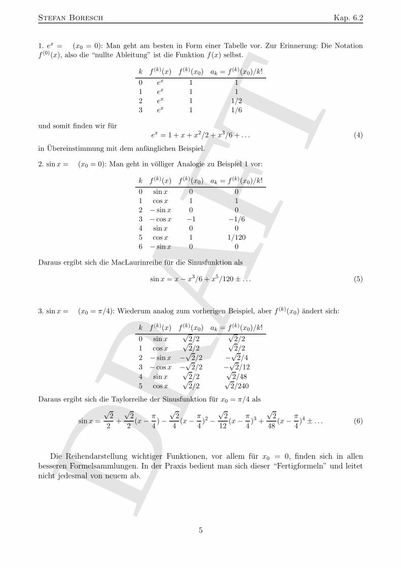
1. ex = (x0 = 0): Man geht am besten in Form einer Tabelle vor. Zur Erinnerung: Die Notationf (0)(x), also die “nullte Ableitung” ist die Funktion f(x) selbst.

k f (k)(x) f (k)(x0) ak = f (k)(x0)/k!

0 ex 1 11 ex 1 12 ex 1 1/23 ex 1 1/6

und somit finden wir furex = 1 + x + x2/2 + x3/6 + . . . (4)

in Ubereinstimmung mit dem anfanglichen Beispiel.

2. sin x = (x0 = 0): Man geht in volliger Analogie zu Beispiel 1 vor:

k f (k)(x) f (k)(x0) ak = f (k)(x0)/k!

0 sin x 0 01 cos x 1 12 − sin x 0 03 − cos x −1 −1/64 sin x 0 05 cos x 1 1/1206 − sin x 0 0

Daraus ergibt sich die MacLaurinreihe fur die Sinusfunktion als

sin x = x − x3/6 + x5/120 ± . . . (5)

3. sin x = (x0 = π/4): Wiederum analog zum vorherigen Beispiel, aber f (k)(x0) andert sich:

k f (k)(x) f (k)(x0) ak = f (k)(x0)/k!

0 sin x√

2/2√

2/2

1 cos x√

2/2√

2/2

2 − sin x −√

2/2 −√

2/4

3 − cos x −√

2/2 −√

2/12

4 sin x√

2/2√

2/48

5 cos x√

2/2√

2/240

Daraus ergibt sich die Taylorreihe der Sinusfunktion fur x0 = π/4 als

sin x =

√2

2+

√2

2(x − π

4) −

√2

4(x − π

4)2 −

√2

12(x − π

4)3 +

√2

48(x − π

4)4 ± . . . (6)

Die Reihendarstellung wichtiger Funktionen, vor allem fur x0 = 0, finden sich in allenbesseren Formelsammlungen. In der Praxis bedient man sich dieser “Fertigformeln” und leitetnicht jedesmal von neuem ab.

5

DR

AFT


6.2 Anmerkungen zum Gultigkeitsbereich

Taylor- und MacLaurinreihen sind nutzliche Werkzeuge, und Sie konnen davon ausgehen, daßGln. 2 bzw. 3 ihre Berechtigung haben. Allerdings ist eine Taylorentwicklung um einen Punktx0 nicht immer fur beliebige Werte von x gultig. Um den Gultigkeitsbereich von Taylorreihenzu bestimmen, muß man sich mit dem Konvergenzverhalten der Reihe beschaftigen, wir habenhierfur nicht genug Zeit, und es sei nicht verheimlicht, daß derartige Untersuchungen nichtimmer einfach sind. Es wurde schon erwahnt, daß wichtige Taylor- und v.a. MacLaurinreihenin Formelsammlungen zu finden sind. Diese Tabellen enthalten immer den Gultigkeitsbereichder jeweiligen Reihe in Form des sogenannten Konvergenzradius. Anwendung einer Taylorreihefur Werte von x außerhalb des Gultigkeitsbereichs der Darstellung ist eine “Todsunde” — einederartige Rechnung (Anwendung) ist schlichtweg Unsinn (ahnlich einer Division durch Null)!Schlagen wir in einer Formelsammlung nach, z.B. [Bartsch S. 195ff]. Wir finden z.B. auf S. 175unten die MacLaurinreihe der Funktion

f(x) = (1 ± x)1/2 = 1 ± 1

2x − 1 · 1

2 · 4x2 ± 1 · 1 · 32 · 4 · 6x3 . . .

plus der Angabe, daß diese Darstellung fur |x| ≤ 1 anwendbar ist. Gleich darunter finden wirdie Reihe fur

f(x) = (1 ± x)−1 = 1 ∓ x + x2 ∓ x3 . . . ,

diese Reihe ist allerdings nur fur |x| < 1 gultig.1 Diese beiden Reihen sind Beispiele von MacLau-rinreihen, die nur innerhalb eines bestimmten Konvergenzradius gultig sind. Es gibt allerdingsviele Funktionen, u.a. ex, sin x und cos x deren Reihendarstellungen fur alle x ∈ R verwendbarist.

Abschließend sei noch angemerkt, daß fur die meisten Funktionen praferentiell die MacLau-rinreihe verwendet wird (also Entwicklung um x0 = 0). Die große Ausnahme ist der Logarith-mus, der an der Stelle 0 nicht definiert ist. Fur ln x verwendet man daher z.B. die Taylorreihean der Stelle x0 = 1 [Bartsch S. 196]

ln x = (x − 1) − (x − 1)2

2+

(x − 1)3

3. . . 0 < x ≤ 2.

6.3 Rechnen mit Potenzreichen

Taylorreihen (MacLaurinreihen) sind Spezialfalle von unendlichen Potenzreihen2 der allgemei-nen Form

A + B (x−x0)+ C (x−x0)2 + . . . = a0 + a1 (x−x0)+ a2 (x−x0)

2 + . . . =∞∑

i=0

ai (x− x0)i. (7)

Solange eine Potenzreihe absolut konvergent ist, darf Sie in vielfaltiger Weise manipuliert wer-den. Diese Voraussetzung, auf die wir hier nicht weiter eingehen konnen, ist automatisch erfullt,

1Es sind diese kleinen Feinheiten (Unterschied zw. |x| ≤ 1 und |x| < 1), die die Bestimmung von Konver-genzradien nichttrivial machen.

2Dies schlagt sich auch unglucklicherweise in Formelsammlungen nieder: Die Definition von Taylor- undMacLaurinreihen finden Sie meist im Kapitel “Differentialrechnung”, Tabellen mit speziellen (MacLaurin) Rei-hen und sonstige Informationen hingegen im Abschnitt “Potenzreihen”.

6

DR

AFT


wenn wir Potenzreihen nur innerhalb ihres Konvergenzradius verwenden. Derartige Manipula-tionen sind u.a. ein wichtiges Hilfsmittel zur raschen Gewinnung von Taylor- und MacLaurinrei-hen als mittels der Definition Gl. 2 moglich ware. In manchen Fallen stellt diese Vorgehensweisesogar den einzig praktikablen Weg dar.3

Der folgende Uberblick beschrankt sich der Einfachheit halber auf MacLaurinreihen, oderallgemeiner Potenzreihen der Form:

A + B x + C x2 + . . . = a0 + a1 x + a2 x2 + . . . =

∞∑

i=0

ai xi. (8)

1) Zwei Potenzreichen werden addiert bzw. subtrahiert, indem man die einzelnen Gliederaddiert (subtrahiert). Es gilt

(a0 + a1x + a2x2 + . . .) + (b0 + b1x + b2x

2 + . . .) = (a0 + b0) + (a1 + b1)x + (a1 + b1)x2 + . . . (9)

bzw.∞∑

i=0

aixi +

∞∑

i=0

bixi =

∞∑

i=0

(ai + bi)xi.

An dieser Stelle gleich eine Anmerkung: Die Wichtigkeit des Konvergenzradius wurde im vor-herigen Abschnitt betont. Wie sieht es mit dem Gultigkeitsbereich einer Potenzreihe (MacLau-rinreihe) aus, die sich aus zwei Potenzreihen wie z.B. in Gl. 9 zusammensetzt? Im Prinzip mußder Konvergenzradius der resultierenden Reihe erneut untersucht werden. Wir beschranken unshier auf folgende “Faustregel”: Der kleinere Konvergenzradius “gewinnt”, d.h., der Konver-genzradius der resultierenden Reihe kann nicht großer sein als der kleinere der Ausgangsreihen.Diese Faustregel ist die obere Grenze des resultierenden Konvergenzradius, dieser kann (z.B.bei verschachtelten Funktionen, s.u.) auch kleiner sein.

Als Anwendung beweisen wir die Eulersche Formel eix = cos x + i sin x: Die Reihen fur ex (Gl. 4)und sinx (Gl. 5) haben wir bereits abgeleitet, die Reihe cos x = 1 − x2/2 + x4/24 ± . . . entnehmenwir der Formelsammlung (z.B. [Bartsch S. 196]. Mit Gl. 4 und t = ix erhalt man ausgehend von derlinken Seite der Eulerschen Formel

eix = et = 1 + t +t2

2+

t3

6+

t4

24+

t5

120+ . . . = 1 + ix +

(ix)2

2+

(ix)3

6+

(ix)4

24+

(ix)5

120+ . . . =

= 1 + ix − x2

2− i

x3

6+

x4

24+ i

x5

120+ . . . = 1 − x2

2+

x4

24+ . . .

︸︷︷︸

cos x

+i(x − x3

6+

x5

120︸︷︷︸

sin x

)= cos x + i sin x

Damit ist die Eulersche Formel bewiesen (oder zumindestens plausibel gemacht — fur einen exak-

ten Beweis mussten wir zeigen, daß die Differentiationsregeln fur die imaginare Zahl ix unverandert

bleiben)

2) Absolut konvergente Potenzreihen konnen gliedweise multipliziert werden. In der Praxis

3Um zu sehen was gemeint ist, versuchen Sie die ersten vier nichtverschwindenden Terme der MacLaurinreihefur f(x) = sin(x2) zu bestimmen.

7

DR

AFT


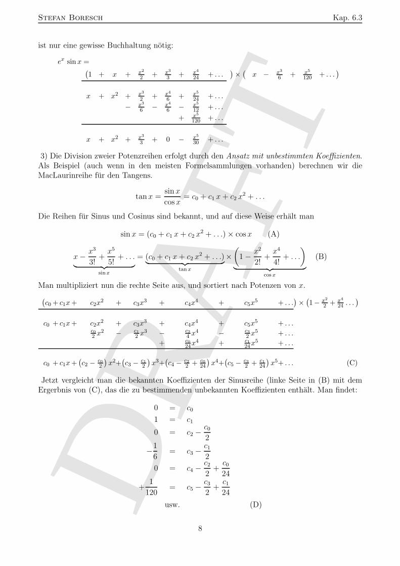
ist nur eine gewisse Buchhaltung notig:

ex sin x =(1 + x + x2

2 + x3

3 + x4

24 + . . .)×

(x − x3

6 + x5

120 + . . .)

x + x2 + x3

2 + x4

6 + x5

24 + . . .

− x3

6 − x4

6 − x5

12 + . . .

+ x5

120 + . . .

x + x2 + x3

3 + 0 − x5

30 + . . .

3) Die Division zweier Potenzreihen erfolgt durch den Ansatz mit unbestimmten Koeffizienten.Als Beispiel (auch wenn in den meisten Formelsammlungen vorhanden) berechnen wir dieMacLaurinreihe fur den Tangens.

tanx =sin x

cos x= c0 + c1 x + c2 x2 + . . .

Die Reihen fur Sinus und Cosinus sind bekannt, und auf diese Weise erhalt man

sin x = (c0 + c1 x + c2 x2 + . . .) × cos x (A)

x − x3

3!+

x5

5!+ . . .

︸︷︷︸

sinx

= (c0 + c1 x + c2 x2 + . . .)︸︷︷︸

tan x

×(

1 − x2

2!+

x4

4!+ . . .

)

︸︷︷︸

cos x

(B)

Man multipliziert nun die rechte Seite aus, und sortiert nach Potenzen von x.

(c0 + c1x + c2x

2 + c3x3 + c4x

4 + c5x5 + . . .

)×

(1− x2

2 + x4

24 . . .)

c0 + c1x + c2x2 + c3x

3 + c4x4 + c5x

5 + . . .c02 x2 − c1

2 x3 − c24 x4 − c3

2 x5 + . . .

+ c024x4 + c1

24x5 + . . .

c0 + c1x +(c2 − c0

2

)x2+

(c3 − c1

2

)x3+

(c4 − c2

2 + c024

)x4+

(c5 − c3

2 + c124

)x5+ . . . (C)

Jetzt vergleicht man die bekannten Koeffizienten der Sinusreihe (linke Seite in (B) mit demErgerbnis von (C), das die zu bestimmenden unbekannten Koeffizienten enthalt. Man findet:

0 = c0

1 = c1

0 = c2 −c0

2

−1

6= c3 −

c1

2

0 = c4 −c2

2+

c0

24

+1

120= c5 −

c3

2+

c1

24

usw. (D)

8

DR

AFT


Daraus erhalt man nach kurzer Rechnung die Koeffizienten und somit die MacLaurinreihe furden Tangens,

tan x = x +1

3x3 +

2

15x5 + . . .

(Dies ist ein Fall, wo der Konvergenzradius der resultierenden Reihe “deutlich” kleiner ist alsder der Ausgangsreihen — obwohl die Reihen fur Sinus und Cosinus fur alle x ∈ R gultig sind,ist der Konvergenzradius des Tangens |x| < π/2.4

4) Die vielleicht nutzlichste Regel in Hinblick auf die Gewinnung neuer MacLaurinreihenbetrifft verknupfte Funktionen, wir illustrieren dies an einem einfachen Beispiel: Gesucht seidie MacLaurinreihenentwicklung von f(x) = sin(x2). Man schreibt jetzt u = x2 und beginntmit der Reihenentwicklung von sin u (Formelsammlung):

sin u = u − u3

3!+

u5

5!− u7

7!± . . .

In diese Reihe setzt man jetzt mit u = x2 ein, und erhalt muhelos

sin(x2) = x2 − x6

3!+

x10

5!− x14

7!± . . .

Der Ausdruck fur u muß kein Ausdruck mit nur endlich vielen Gliedern sein, wie in obigen Beispiel.Z.B. fur f(x) = esinx startet man mit

eu = 1 + u +u2

2+

u3

3!+ . . .

und setzt dann auf der rechten Seite fur u = sin x = x−x3/3!+x5/5!± . . . ein. Die Vereinfachung des

resultierenden Ausdrucks wird allerdings rasch ziemlich muhsam.

5) Absolut konvergente Potenzreihen durfen gliedweise differenziert und integriert werden.Aus der Formelsammlung ([Bartsch S. 195]) entnehmen wir

1

1 − x= 1 + x + x2 + x3 + . . . |x| < 1

Durch Differenzieren der linken und rechten Seite finden wir sofort die Potenzreihendarstellungvon (1 − x)−2

1

(1 − x)2= 1 + 2x + 3x2 + . . . |x| < 1

mit gleichem Konvergenzradius.

Im Kapitel uber Integration haben wir festgestellt, daß wir Funktionen wie ex2, sin(x2) und

cos(x2) keine Stammfunktionen finden konnen, obwohl diese existieren mussen. Die Potenz-reihendarstellungen (MacLaurinreihen) dieser Stammfunktionen kann man jedoch sofort durchgliedweise Integration erhalten. Gesucht sei z.B.

∫

dx ex2

4Dies ist naturlich nicht wirklich uberraschend, denn fur x = ±π/2 wird der Nenner 0!

9

DR

AFT


Wir bestimmen zunachst die MacLaurinreihe fur ex2. Mit u = x2 finden wir

ex2

= eu = 1 + u +u2

2+

u3

3!+ . . . = 1 + x2 +

x4

2+

6

3!+ . . .

und daraus sofort∫

dx ex2

=

∫

dx (1 + x2 +x4

2+

x6

3!+ . . .) = x +

x3

3+

x5

10+

x7

42+ . . .

6.4 Zur Verwendung von Taylorreihen

Taylorreihen vermitteln einerseits einen Einblick, was sogenannte transzendentale Funktionen(ex, sin x usw.) eigentlich sind bzw. wie man Sie im Prinzip (naherungsweise5) berechnen konnte.Weiters tauchen Taylorreihen immer wieder in physikalischen, chemischen oder mathematischenHerleitungen auf, ohne daß dies speziell erwahnt wird. Besonders “beliebt” sind in diesemZusammenhang die lineare Naherung, d.h.,

f(x) ≈ f(x0) + (x − x0)f′(x0),

sowie die quadratische Naherung, d.h.,

f(x) ≈ f(x0) + (x − x0)f′(x0) +

(x − x0)2

2f ′′(x0).

Letztere wird besonders dann verwendet, wenn f ′(x0) = 0. “Mutiert” in einer Herleitung z.B.ein ex “fur kleine x” in 1 + x, so wurden die beiden ersten Glieder der MacLaurinreihe derExponentialfunktion verwendet. Ahnliche Nahrerungen (immer nur gultig fur “kleine x”) sindz.B. sin x ≈ x, 1/(1 + x) ≈ 1 − x usw. (siehe auch z.B. [Bartsch S. 198]).

Taylorreihen lassen sich auch zur Grenzwertberechnung verwenden. Dies ist besonders dann nutz-lich, wenn man im Zuge der Grenzwertberechnung auf unbestimmte Ausdrucke der Form 0

0 oder ∞

∞

stoßt. Beispiel:

limx→0

1 − cos 2x

e3x − 1 − 3x= lim

x→0

1 −(

1 − 4x2

2 + 16x4

24 . . .)

(

1 + 3x + 9x2

2 . . .)

− 1 − 3x=

= lim x → 0x2

(2 − 16

24x2 . . .)

x2(

92 + 27

6 x . . .) =

4

9

Alternativ kann man naturlich auch die l’Hopitalsche Regel anwenden: Stoßt man bei einer Grenz-wertberechnung auf einen unbestimmten Ausdruck 0

0 oder ∞

∞, so kann differenziert man Zahler und

Nenner so lange bis der Grenzwert berechnet werden kann oder klar ist, daß der Grenzwert nichtexistiert. Fur das obige Beispiel

limx→0

0︷︸︸︷

1 − cos 2x

e3x − 1 − 3x︸︷︷︸

0

= limx→0

0︷︸︸︷

2 sin 2x

3e3x − 3︸︷︷︸

0

= limx→0

4 cos x

9e3x=

4

9.

5Naherungsweise deshalb, weil Sie immer nur endlich viele Terme berechnen konnen. In der numerischenMathematik kennt man viele Tricks um die Konvergenz von Reihen zu beschleunigen. Mit beinahe an Sicherheitgrenzender Wahrscheinlichkeit verwendet Ihr Taschenrechnerkeine Taylorreihen, um Sinus, Cosinus usw. zuberechnen, das Prinzip verdeutlichen sie aber nicht schlecht.

10

DR

AFT


Die Grenzwertberechnung mittels Taylorreihen wird im Vergleich zur l’Hopitalschen Regel um so

effizienter, je ofter man bei letzterer Zahler und Nenner differenzieren muß.

7 Anmerkungen zu Funktionen mehrerer Veranderlicher

Funktionen einer Veranderlichen, also unser “gewohntes” f(x), sind in den Naturwissenschafteneher die Ausnahme denn die Regel. Es sei nochmals an das ideale Gasgesetz erinnert,

pV = nRT,

aus dem sich jede der vier Veranderlichen, Druck p, Volumen V , Molmenge n und TemperaturT , jeweils als Funktion der drei anderen Variablen ausdrucken laßt, z.B.

p = p(V, n, T ) =nRT

V

usw. Ein weiteres Beispiel ist die molekularmechanische Beschreibung von Biomolekulen. EinProtein besteht aus N Atomen. Jedes dieser Atome hat eine Position im Raum, (xi, yi, zi). DieGesamtenergie E des Proteins ist eine Funktion aller Atomkoordinaten, d.h.,

E = E(x1, y1, z1, x2, y2, z2, . . . , xN , yN , zN)

ist eine Funktion von 3N Variablen, wobei N einige Hundert bis einige Tausend betragt.

-2 -1 0 1 2

-2

-1

0

1

2

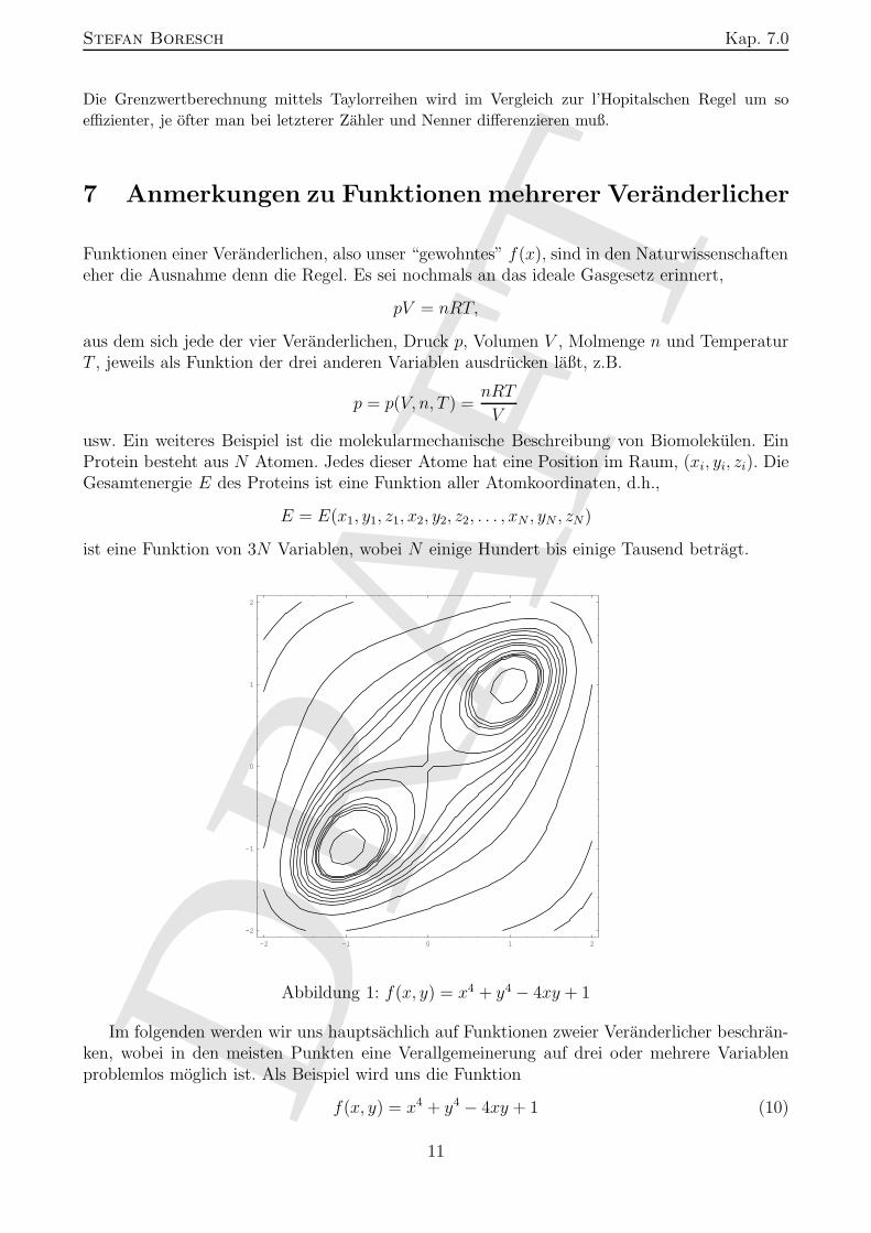
Abbildung 1: f(x, y) = x4 + y4 − 4xy + 1

Im folgenden werden wir uns hauptsachlich auf Funktionen zweier Veranderlicher beschran-ken, wobei in den meisten Punkten eine Verallgemeinerung auf drei oder mehrere Variablenproblemlos moglich ist. Als Beispiel wird uns die Funktion

f(x, y) = x4 + y4 − 4xy + 1 (10)

11

DR

AFT


dienen. Funktionswerte berechnet man fur ein Wertepaar (x, y) durch Einsetzen in die Funkti-onsgleichung. In unserem Beispiel ist daher f(0, 0) = 1, f(1, 2) = 14 + 24 − 4 × 1 × 2 + 1 = 10,f(−1, 1) = 7 usw. Wahrend das Ausrechnen von Funktionswerten kein Problem ist, ist die gra-phische Darstellung eine etwas großere Herausforderung. Fur zwei Veranderliche kann man denFunktionswert f(x, y) als z-Wert in einem dreidimensionalen kartesischen Koordinatensystemdarstellen. Dies ist zwar optisch recht ansprechend, wird aber rasch unubersichtlich. Eine zweiteMoglichkeit besteht in der Verwendung von Kontour- oder Hohenschichtlinien. Ahnlich wie ineiner Landkarte die Punkte gleicher Hohe durch Linien verbunden werden, stellt man die Funk-tion durch Linien gleicher Funktionswerte dar. Fur unsere Beispielsfunktion ist dies in Fig. 1illustriert. Derartige Plots mussen wie Landkarten interpretiert werden. Man sieht also, daß bei(−1,−1) und (1, 1) Maxima (“Gipfel”) oder Minima (“Tal”) vorliegen, und daß bei (0, 0) einUbergang (“Sattel”) zwischen diesen beiden Extremstellen vorliegt. Das systematische Findenvon Maxima und Minima werden wir in Abschnitt 7.3 behandeln.

Ein wichtiger Unterschied zwischen Funktionen zweier Veranderlicher und Funktionen vonmehr als zwei Veranderlichen besteht darin, daß in letzterem Fall keine einfache graphischeDarstellung mehr moglich ist.

Bei Funktionen in einer Veranderlichen haben wir uns recht detailliert mit der Definitions-menge und der Frage der Stetigkeit auseinandergesetzt. Die Prinzipien, die wir dort gefundenhaben, behalten auch fur mehrdimensionale Funktionen ihre Gultigkeit. Aus der Definitions-menge sind alle jene Punkte (Variablenpaare, -tripel usw.) auszuschließen, die auf eine verboteneOperation fuhren wurden oder den Funktionswert komplex machen wurden. Z.B. fur die Funk-tion f(x, y, z) = x+y

zmussen alle (x, y, z)-Tripel mit z = 0 ausgeschlossen werden, um eine

Division durch Null zu vermeiden. Der Begriff der Stetigkeit laßt sich anschaulich immer nocham besten durch das Adjektiv “glatt” charakterisieren. So ist z.B. die Funktion

f(x, y) =

{

x + y x 6= 0 und y 6= 0,

5 x = y = 0

im Punkt (0, 0) unstetig, da die Funktion den Wert f(x → 0, y → 0) → 0 anstrebt, im Punktselbst aber auf f(0, 0) = 5 springt. In dieser Betrachtung ist naturlich wieder ein Grenzwertverborgen. Zu Grenzwerten nur so viel: Prinzipiell andert sich nichts gegenuber Grenzwertenfur Funktionen einer Veranderlichen. Die Existenz eines Grenzwerts im mehrdimensionalen Fallbedingt jedoch zusatzlich, daß derselbe Wert angenommen wird, unabhangig von der Richtungaus der man sich dem fraglichen Punkt nahert. So strebt im obigen Beispiel der Funktionswertgegen 0, egal ob man zuerst x → 0 gegen Null und dann y → 0 gegen 0 gehen laßt, oderumgekehrt, usw. Da dieser Grenzwert limx→0

y→0[x+y] = 0 nicht mit dem Funktionswert in diesem

Punkt f(0, 0) = 5 ubereinstimmt, ist die Funktion in diesem Punkt jedoch nicht stetig.

7.1 Partielle Ableitungen

Untersucht man Funktionen mehrerer Veranderlicher ohne Plan, so wird man leicht “schwind-lig”. Der einfachste systematische Ansatz besteht darin, sich immer auf eine Variable zu konzen-trieren, und die andere(n) Variable(n) konstant zu halten. Dies entspricht der experimentellenPraxis. Ist man an einer Reaktionsgeschwindigkeit als Funktion der Konzentration interessiert,so wird man alle anderen Bedingungen (Variablen), insbesondere die Temperatur konstant zu

12

DR

AFT


halten trachten. Will man hingegen die Reaktionsgeschwindigkeit als Funktion der Temperaturmessen, so wird man immer mit den selben (Start)konzentrationen arbeiten.

Betrachten wir als Beispiel unsere Funktion Gl. 10 und setzen einmal x = a und einmaly = b, wobei a und b beliebige Konstanten ∈ R seien (fur diese Beispielsfunktion gibt es keinerleiEinschrankungen der Definitionsmenge).

f(x = a, y) = f1(y) = a4 + y4 − 4ay + 1f(x, y = b) = f2(x) = x4 + b4 − 4bx + 1

Wir erhalten zwei gewohnliche eindimensionale Funktionen f1(y), f2(x), die jetzt ganz normalnach der jeweiligen Variablen x bzw. y abgeleitet werden konnen:

f ′

1(y) = 4y3 − 4a = f ′(x = a, y)

f ′

2(x) = 4x3 − 4b = f ′(x, y = b)

Die jeweils letzte Identitat auf der rechten Seite soll andeuten, daß es sich bei f ′

1(y) auch um dieAbleitung von f(x, y) nach y handelt, wenn der x-Wert bei x = a festhalten wird, und analogfur f ′

2(x).

Es sei nochmals betont, daß wir keinerlei Einschrankungen bezuglich a und b gemacht haben.In diesem Sinn kann man a und b wieder durch x und y ersetzen, soferne man vereinbart, daßfur die Durchfuhrung der Ableitung diese jeweils nichtinteressierenden Variablen x = a ∈ R,y = b ∈ R als konstant betrachtet werden. Diese Vorgehensweise fuhrt auf das Konzept derpartiellen Ableitung. Die partiellen Ableitungen in unserem Beispiel (Gl. 10 lauten daher:

∂f(x, y)

∂x= 4x3 − 4y = fx(x, y) = fx

∂f(x, y)

∂y= 4y3 − 4x = fy(x, y) = fy

Gegenuber den normalen Ableitungen andert sich die Notation etwas. In der LeibnizschenSchreibweise ersatzt man das d in d

dxdurch das stilisierte ∂ und schreibt (fur die partielle Ab-

leitung nach x) ∂∂x

, und an Stelle des ′ in f ′ schreibt man als Subskript die Variable, nach derabgeleitet wird, z.B. fy. Die praktische Rechenregel lautet: Man betrachte die nichtinteressie-rende Variable (die nichtinteressierenden Variablen) als Konstante, und leite ansonsten ganzgewohnlich ab.

Im eindimensionalen Fall war die Interpretation der Ableitung die Rate der Anderung vonf(x) als Funktion von x. Die partielle Ableitung nach z.B. x einer Funktion f(x, y, z, . . .) kannals die Rate der Anderung von f(x, y, z, . . .) in Abhangigkeit von x bei konstantem y, z usw.aufgefasst werden. Etwas formaler laßt sich das durch folgende Definitionen (fur den zweidi-mensionalen Fall) ausrucken:

∂f(x, y)

∂x= lim

∆x→0

f(x + ∆x, y) − f(x, y)

∆x

∂f(x, y)

∂y= lim

∆y→0

f(x, y + ∆y) − f(x, y)

∆y(11)

13

DR

AFT


7.2 Hohere partielle Ableitungen — Satz von Schwarz

Wir haben eben fur unsere Beispielsfunktion Gl. 10, f(x, y) = x4 + y4 − 4xy + 1, die partiellenAbleitungen

fx = 4x3 − 4y fy = 4y3 − 4x

berechnet. Nachdem diese wiederum Funktionen von x und y sind, kann man weiter (partiell)ableiten, und findet

fxx =∂2f

∂x2= 12x2

fyy =∂2f

∂y2= 12y2

die zweiten partiellen Ableitung nach x bzw. y. Man kann aber naturlich auch fx nach y ableiten,d.h.

∂

∂yfx =

∂

∂y

(∂f

∂x

)

=∂2f

∂x∂y= fxy = −4.

Man spricht von der gemischten partiellen Ableitung, wobei zuerst nach x, dann nach y abge-leitet wurde. Es ist naturlich genauso moglich, fy nach x abzuleiten,

∂

∂xfy =

∂

∂x

(∂f

∂y

)

=∂2f

∂y∂x= fyx = −4.

Diese gemischten partiellen Ableitungen sind etwas fundamental Neues, was es im eindimen-sionalen Fall nicht gab und geben konnte. Fur die partiellen Ableitungen gilt jetzt folgenderwichtiger Zusammenhang (in der deutschen Literatur als Satz von Schwarz, in der englischen Li-teratur als Clairaut’s Theorem bezeichnet): Besitzt f(x, y) im Innern eines gewissen Bereichs,a < x < b, c < y < d, stetige Ableitungen fxy und fyx, so sind diese Ableitungen in alleninneren Punkten des Bereichs gleich, d.h. es gilt

fxy = fyx, a < x < b, c < y < d (12)

Mit anderen Worten, das Resultat der Differentiation hangt (unter den oben genannten Voraus-setzungen) nicht von der Reihenfolge ab, in der die (partiellen) Differentiationen durchgefuhrtwerden. Diese Ergebnis gilt auch fur hohere Ableitungen als auch fur Funktionen mit mehr alszwei Veranderlichen, so gilt z.B. fur die Funktion f(x, y, z, t)

fxxyzt = fytzxx = ftzyxx = . . .usw.

Beispiel: Fur f(x, y) = e2x−y

y findet man (die Details bleiben Ihnen uberlassen!)

fx =2e2x−y

yfy = −e2x−y(y + 1)

y2.

Eine kurze Rechnung zeigt jetzt, daß

fxy =y 2e2x−y(−1) − 1 · 2e2x−y

y2= fyx = −y + 1

y22e2x−y

14

DR

AFT


7.3 Stationare Punkte fur Funktionen zweier Veranderlicher

Eine Hauptanwendung der Differentialrechnung in einer Veranderlichen war die Bestimmungvon Minima, Maxima und Wendepunkte von Funktionen, d.h., von Punkten einer Funktionan denen sich das Verhalten der Funktion andert. Wir wollen derartige Untersuchungen jetztauch fur Funktionen zweier Veranderlicher durchfuhren, und kurz auch auf Funktionen mitmehr als zwei Veranderlichen eingehen. Maxima, Minima, und die sogenannten Sattelpunkte(die “Wendepunkte” im mehrdimensionalen Fall) bezeichnet man auch als stationarer Punkte.

Eine Funktion f(x, y) habe im Punkt (a, b) ein Maximum (Minimum). Dann gilt in einergewissen Umgebung um (a, b), daß

∆f = f(a + ∆x, b + ∆y) − f(a, b)

{

≤ 0 (Maximum)

≥ 0 (Minimum)

(Dies folgt ganz allgemein aus den Eigenschaften eines Maximums oder Minimus ohne jeglicheDifferentialrechnung). Gewinnt man jetzt wie im Abschnitt 7.1 aus f(x, y) wieder zwei eindi-mensionale Hilfsfunktionen f1(x, b) und f2(a, y), (wobei jetzt a und b die x- bzw. y− Werte desPunkts (a, b) sind, in denen f(x, y) ein Maximum (Minimum) annimmt), so muß ganz sichergelten, daß

f1(x, b) hat fur x = a ein Maximum (Minimum), d.h. df1(x,b)dx

∣∣∣x=a

= 0

f2(a, y) hat fur y = b ein Maximum (Minimum), d.h. df2(a,y)dy

∣∣∣y=b

= 0

Ubersetzt man dies wieder in die Sprache der partiellen Ableitungen, so findet man als notwendi-ges Kriterium fur die Existenz eines Maximums oder Minimums, daß die partiellen Ableitungensimultan verschwinden mussen, d.h.

fx(x, y) = 0

fy(x, y) = 0 (13)

Dieses Ergebnis laßt sich sofort auf Funktionen mehrerer Veranderlicher verallgemeinern. Dienotwendige Bedingungen fur das Vorhandensein stationarer Punkte einer Funktion f(x, y, z, . . .)ist das simultane Verschwinden aller ihrer ersten partiellen Ableitungen

fx(x, y, z, . . .) = 0

fy(x, y, z, . . .) = 0

fz(x, y, z, . . .) = 0

usw.

Kriterium Gl. 13 ist ein notwendiges, aber kein hinreichendes Kriterium fur ein Maximumoder ein Minimum einer Funktion f(x, y). Wir mussen zunachst ausschließen, daß es sich nichtum einen “Wendepunkt” (den man im mehrdimensionalen Fall Sattelpunkt nennt) handelt,und weiters mussen wir noch zwischen Maxima und Minima unterscheiden. Wir uberlegenuns zunachst in Analogie zum eindimensionalen Fall ein paar Spezialfalle, danach geben wir(ohne Beweis) die allgemeine Regel an. (i) Bei Funktionen einer Veranderlichen ist Vorsicht

15

DR

AFT


geboten, wenn an einem Punkt x0 sowohl erste als auch zweite Ableitung verschwinden, d.h.wenn f ′(x0) = f ′′(x0) = 0 gilt. Auch fur Funktionen zweier Veranderlicher gilt: Verschwindetzumindestens eine der reinen zweiten partiellen Ableitungen fxx bzw. fyy an einem Punkt(x0, y0), so handelt es sich bei diesem Punkt fur gewohnlich nicht um eine Extremstelle undspezielle Tests sind notig. (ii) Im Eindimensionalen gibt das Vorzeichen der zweiten Ableitungan einer Kanditatenstelle Auskunft daruber, ob es sich bei dieser Stelle um ein Maximum oderMinimum handelt. Analoges gilt fur Funktionen zweier Veranderlicher. Je nach Vorzeichen vonfxx bzw. fyy im Kandidatenpunkt (x0, y0) handelt es sich um ein Maximum (fxx < 0 undfyy < 0) oder ein Minimum (fxx > 0 und fyy > 0). Insbesondere aber muß das Vorzeichender zweiten Ableitungen ubereinstimmen, sonst ist (x0, y0) mit Sicherheit keine Extremstelle,sondern ein Sattelpunkt.

Nach diesen Vorbemerkungen kommen wir jetzt zur allgemeinen Regel. Man betrachtet (furjede Kanditatenstelle (x0,i, y0,i)) eine Große ∆ (oder D), die sogenannte Diskriminante:

∆(x, y) = fxx fyy − (fxy)2 (14)

Ist an einer Kanditatenstelle (x0,i, y0,i) die Diskriminante ∆(x0,i, y0,i) > 0, so handelt es sichum eine Extremstelle und das Vorzeichen der zweiten Ableitung bestimmt (vgl. (ii) im vorigenAbsatz), ob es sich um ein Maximum (fxx(x0,i, y0,i) < 0) oder ein Minimum (fxx(x0,i, y0,i) > 0)handelt. Gilt hingegen ∆(x0,i, y0,i) < 0, so handelt es sich um einen Sattelpunkt. Tritt schließlichder Fall ∆ = 0 ein, so muß die Entscheidung zwischen Maximum, Minimum oder Sattelpunktmit anderen, hier nicht behandelbaren Methoden getroffen werden. Wenn Sie sich die Vorzei-chenregeln fur ∆ durch den Kopf gehen lassen, so sehen Sie, daß die allgemeine Regel unsereSpezialfalle (i) und (ii) miteinschließt.

Eine Verallgemeinerung der eben aufgestellten Regel zur Unterscheidung zwischen Minima,Maxima und Sattelpunkten fur Funktionen von mehr als zwei Variabeln ist außerst muhsam.In der Praxis bestimmt man meist die Kanditatenstelle(n) und vergewissert sich durch Stich-proben, ob es sich um ein Maximum oder ein Minimum handelt.

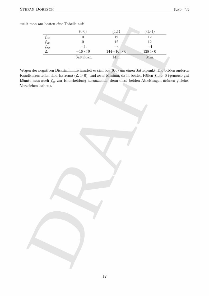
Beispiel: Gesucht sind die stationaren Punkte der Funktion Gl. 10, f(x, y) = x4 + y4 − 4xy + 1. Wirkennen bereits alle benotigten Ableitungen: fx = 4x3 − 4y, fy = 4y3 − 4x, fxx = 12x2, fyy = 12y2,fxy = fyx = −4. Gemaß Kriterium Gl. 13 benotigen wir zunachst die Losung des Gleichungssystems:

fx = 4x3 − 4y = 0 (I)

fy = 4y3 − 4x = 0 (II)

Es folgt z.B. aus (I) y = x3. Einsetzen in (II) fuhrt auf

x9 − x = x(x8 − 1) = 0 (*)

Gl. (*) hat die Losungen x1 = 0, x2 = +1 und x3 = −1. Daraus ergeben sich mit y = x3 die dazugehori-gen y-Werte y1 = 0, y2 = +1 und y3 = −1. Die Kanditatenstellen (Losungen des Gleichungssystems(I), (II)) sind also (0, 0), (1, 1) und (−1,−1).

Fur diese Kanditatenstellen ist jetzt das Verhalten von ∆ (Gl. 14) zu untersuchen. In der Praxis

16

DR

AFT


stellt man am besten eine Tabelle auf:

(0,0) (1,1) (-1,-1)

fxx 0 12 12fyy 0 12 12fxy −4 −4 −4∆ −16 < 0 144−16 > 0 128 > 0

Sattelpkt. Min. Min.

Wegen der negativen Diskriminante handelt es sich bei (0, 0) um einen Sattelpunkt. Die beiden anderen

Kanditatenstellen sind Extrema (∆ > 0), und zwar Minima, da in beiden Fallen fxx > 0 (genauso gut

konnte man auch fyy zur Entscheidung heranziehen, denn diese beiden Ableitungen mussen gleiches

Vorzeichen haben).

17

DR

AFT

Verwendete Literatur

• E. Steiner “The Chemistry Maths Book”, Oxford Science, Oxford, New York 1996.

• H. G. Zachmann “Mathematik fur Chemiker”, 4. Auflage, Verlag Chemie, Weinheim, DeerfieldBeach, Basel 1981.

• W. I. Smirnow “Lehrbuch der hoheren Mathematik”, Teil I, 16. Auflage, Verlag Harri Deusch,Frankfurt, 1971.

Auflistung von Anderungen — “revision history”

Dezember 2003/Janner 2004 Erste Rohfassung.

GNU Free Documentation License

GNU Free Documentation LicenseVersion 1.2, November 2002

Copyright (C) 2000,2001,2002 Free Software Foundation, Inc.59 Temple Place, Suite 330, Boston, MA 02111-1307 USA

Everyone is permitted to copy and distribute verbatim copiesof this license document, but changing it is not allowed.

0. PREAMBLE

The purpose of this License is to make a manual, textbook, or other functional and useful document “free” in the sense of freedom: to assureeveryone the effective freedom to copy and redistribute it, with or without modifying it, either commercially or noncommercially. Secondarily, thisLicense preserves for the author and publisher a way to get credit for their work, while not being considered responsible for modifications made byothers.

This License is a kind of “copyleft”, which means that derivative works of the document must themselves be free in the same sense. It complementsthe GNU General Public License, which is a copyleft license designed for free software.

We have designed this License in order to use it for manuals for free software, because free software needs free documentation: a free programshould come with manuals providing the same freedoms that the software does. But this License is not limited to software manuals; it can be used forany textual work, regardless of subject matter or whether it is published as a printed book. We recommend this License principally for works whosepurpose is instruction or reference.

1. APPLICABILITY AND DEFINITIONS

This License applies to any manual or other work, in any medium, that contains a notice placed by the copyright holder saying it can be distributedunder the terms of this License. Such a notice grants a world-wide, royalty-free license, unlimited in duration, to use that work under the conditionsstated herein. The “”Document”, below, refers to any such manual or work. Any member of the public is a licensee, and is addressed as “you”. Youaccept the license if you copy, modify or distribute the work in a way requiring permission under copyright law.

A “Modified Version” of the Document means any work containing the Document or a portion of it, either copied verbatim, or with modificationsand/or translated into another language.

A “Secondary Section” is a named appendix or a front-matter section of the Document that deals exclusively with the relationship of the publishersor authors of the Document to the Document’s overall subject (or to related matters) and contains nothing that could fall directly within that overallsubject. (Thus, if the Document is in part a textbook of mathematics, a Secondary Section may not explain any mathematics.) The relationship could bea matter of historical connection with the subject or with related matters, or of legal, commercial, philosophical, ethical or political position regardingthem.

The “Invariant Sections” are certain Secondary Sections whose titles are designated, as being those of Invariant Sections, in the notice that saysthat the Document is released under this License. If a section does not fit the above definition of Secondary then it is not allowed to be designated asInvariant. The Document may contain zero Invariant Sections. If the Document does not identify any Invariant Sections then there are none.

The “Cover Texts” are certain short passages of text that are listed, as Front-Cover Texts or Back-Cover Texts, in the notice that says that theDocument is released under this License. A Front-Cover Text may be at most 5 words, and a Back-Cover Text may be at most 25 words.

A “Transparent” copy of the Document means a machine-readable copy, represented in a format whose specification is available to the generalpublic, that is suitable for revising the document straightforwardly with generic text editors or (for images composed of pixels) generic paint programsor (for drawings) some widely available drawing editor, and that is suitable for input to text formatters or for automatic translation to a variety offormats suitable for input to text formatters. A copy made in an otherwise Transparent file format whose markup, or absence of markup, has beenarranged to thwart or discourage subsequent modification by readers is not Transparent. An image format is not Transparent if used for any substantialamount of text. A copy that is not “Transparent” is called “Opaque”.

Examples of suitable formats for Transparent copies include plain ASCII without markup, Texinfo input format, LaTeX input format, SGMLor XML using a publicly available DTD, and standard-conforming simple HTML, PostScript or PDF designed for human modification. Examples oftransparent image formats include PNG, XCF and JPG. Opaque formats include proprietary formats that can be read and edited only by proprietaryword processors, SGML or XML for which the DTD and/or processing tools are not generally available, and the machine-generated HTML, PostScriptor PDF produced by some word processors for output purposes only.

The “Title Page” means, for a printed book, the title page itself, plus such following pages as are needed to hold, legibly, the material this Licenserequires to appear in the title page. For works in formats which do not have any title page as such, “Title Page” means the text near the most prominentappearance of the work’s title, preceding the beginning of the body of the text.

A section “Entitled XYZ” means a named subunit of the Document whose title either is precisely XYZ or contains XYZ in parentheses following textthat translates XYZ in another language. (Here XYZ stands for a specific section name mentioned below, such as “Acknowledgements”, “Dedications”,

18

DR

AFT

“Endorsements”, or “History”.) To “Preserve the Title” of such a section when you modify the Document means that it remains a section “EntitledXYZ” according to this definition.

The Document may include Warranty Disclaimers next to the notice which states that this License applies to the Document. These WarrantyDisclaimers are considered to be included by reference in this License, but only as regards disclaiming warranties: any other implication that theseWarranty Disclaimers may have is void and has no effect on the meaning of this License.

2. VERBATIM COPYING

You may copy and distribute the Document in any medium, either commercially or noncommercially, provided that this License, the copyrightnotices, and the license notice saying this License applies to the Document are reproduced in all copies, and that you add no other conditions whatsoeverto those of this License. You may not use technical measures to obstruct or control the reading or further copying of the copies you make or distribute.However, you may accept compensation in exchange for copies. If you distribute a large enough number of copies you must also follow the conditionsin section 3.

You may also lend copies, under the same conditions stated above, and you may publicly display copies.

3. COPYING IN QUANTITY

If you publish printed copies (or copies in media that commonly have printed covers) of the Document, numbering more than 100, and theDocument’s license notice requires Cover Texts, you must enclose the copies in covers that carry, clearly and legibly, all these Cover Texts: Front-CoverTexts on the front cover, and Back-Cover Texts on the back cover. Both covers must also clearly and legibly identify you as the publisher of thesecopies. The front cover must present the full title with all words of the title equally prominent and visible. You may add other material on the coversin addition. Copying with changes limited to the covers, as long as they preserve the title of the Document and satisfy these conditions, can be treatedas verbatim copying in other respects.

If the required texts for either cover are too voluminous to fit legibly, you should put the first ones listed (as many as fit reasonably) on the actualcover, and continue the rest onto adjacent pages.

If you publish or distribute Opaque copies of the Document numbering more than 100, you must either include a machine-readable Transparentcopy along with each Opaque copy, or state in or with each Opaque copy a computer-network location from which the general network-using publichas access to download using public-standard network protocols a complete Transparent copy of the Document, free of added material. If you use thelatter option, you must take reasonably prudent steps, when you begin distribution of Opaque copies in quantity, to ensure that this Transparent copywill remain thus accessible at the stated location until at least one year after the last time you distribute an Opaque copy (directly or through youragents or retailers) of that edition to the public.

It is requested, but not required, that you contact the authors of the Document well before redistributing any large number of copies, to givethem a chance to provide you with an updated version of the Document.

4. MODIFICATIONS

You may copy and distribute a Modified Version of the Document under the conditions of sections 2 and 3 above, provided that you release theModified Version under precisely this License, with the Modified Version filling the role of the Document, thus licensing distribution and modificationof the Modified Version to whoever possesses a copy of it. In addition, you must do these things in the Modified Version:

A. Use in the Title Page (and on the covers, if any) a title distinct from that of the Document, and from those of previous versions (which should,if there were any, be listed in the History section of the Document). You may use the same title as a previous version if the original publisher of thatversion gives permission.

B. List on the Title Page, as authors, one or more persons or entities responsible for authorship of the modifications in the Modified Version,together with at least five of the principal authors of the Document (all of its principal authors, if it has fewer than five), unless they release you fromthis requirement.

C. State on the Title page the name of the publisher of the Modified Version, as the publisher.

D. Preserve all the copyright notices of the Document.

E. Add an appropriate copyright notice for your modifications adjacent to the other copyright notices.

F. Include, immediately after the copyright notices, a license notice giving the public permission to use the Modified Version under the terms ofthis License, in the form shown in the Addendum below.

G. Preserve in that license notice the full lists of Invariant Sections and required Cover Texts given in the Document’s license notice.

H. Include an unaltered copy of this License.

I. Preserve the section Entitled “History”, Preserve its Title, and add to it an item stating at least the title, year, new authors, and publisher ofthe Modified Version as given on the Title Page. If there is no section Entitled “History” in the Document, create one stating the title, year, authors,and publisher of the Document as given on its Title Page, then add an item describing the Modified Version as stated in the previous sentence.

J. Preserve the network location, if any, given in the Document for public access to a Transparent copy of the Document, and likewise the networklocations given in the Document for previous versions it was based on. These may be placed in the “History” section. You may omit a network locationfor a work that was published at least four years before the Document itself, or if the original publisher of the version it refers to gives permission.

K. For any section Entitled “Acknowledgements” or “Dedications”, Preserve the Title of the section, and preserve in the section all the substanceand tone of each of the contributor acknowledgements and/or dedications given therein.

L. Preserve all the Invariant Sections of the Document, unaltered in their text and in their titles. Section numbers or the equivalent are notconsidered part of the section titles.

M. Delete any section Entitled “Endorsements”. Such a section may not be included in the Modified Version.

N. Do not retitle any existing section to be Entitled “Endorsements” or to conflict in title with any Invariant Section.

O. Preserve any Warranty Disclaimers.

If the Modified Version includes new front-matter sections or appendices that qualify as Secondary Sections and contain no material copied fromthe Document, you may at your option designate some or all of these sections as invariant. To do this, add their titles to the list of Invariant Sectionsin the Modified Version’s license notice. These titles must be distinct from any other section titles.

You may add a section Entitled “Endorsements”, provided it contains nothing but endorsements of your Modified Version by various parties–forexample, statements of peer review or that the text has been approved by an organization as the authoritative definition of a standard.

You may add a passage of up to five words as a Front-Cover Text, and a passage of up to 25 words as a Back-Cover Text, to the end of the list ofCover Texts in the Modified Version. Only one passage of Front-Cover Text and one of Back-Cover Text may be added by (or through arrangementsmade by) any one entity. If the Document already includes a cover text for the same cover, previously added by you or by arrangement made by the

19

DR

AFT

same entity you are acting on behalf of, you may not add another; but you may replace the old one, on explicit permission from the previous publisherthat added the old one.

The author(s) and publisher(s) of the Document do not by this License give permission to use their names for publicity for or to assert or implyendorsement of any Modified Version.

5. COMBINING DOCUMENTS

You may combine the Document with other documents released under this License, under the terms defined in section 4 above for modifiedversions, provided that you include in the combination all of the Invariant Sections of all of the original documents, unmodified, and list them all asInvariant Sections of your combined work in its license notice, and that you preserve all their Warranty Disclaimers.

The combined work need only contain one copy of this License, and multiple identical Invariant Sections may be replaced with a single copy. Ifthere are multiple Invariant Sections with the same name but different contents, make the title of each such section unique by adding at the end ofit, in parentheses, the name of the original author or publisher of that section if known, or else a unique number. Make the same adjustment to thesection titles in the list of Invariant Sections in the license notice of the combined work.

In the combination, you must combine any sections Entitled “History” in the various original documents, forming one section Entitled “Hi-story”; likewise combine any sections Entitled “Acknowledgements”, and any sections Entitled “Dedications”. You must delete all sections Entitled“Endorsements”.

6. COLLECTIONS OF DOCUMENTS

You may make a collection consisting of the Document and other documents released under this License, and replace the individual copies of thisLicense in the various documents with a single copy that is included in the collection, provided that you follow the rules of this License for verbatimcopying of each of the documents in all other respects.

You may extract a single document from such a collection, and distribute it individually under this License, provided you insert a copy of thisLicense into the extracted document, and follow this License in all other respects regarding verbatim copying of that document.

7. AGGREGATION WITH INDEPENDENT WORKS

A compilation of the Document or its derivatives with other separate and independent documents or works, in or on a volume of a storage ordistribution medium, is called an “aggregate” if the copyright resulting from the compilation is not used to limit the legal rights of the compilation’susers beyond what the individual works permit. When the Document is included an aggregate, this License does not apply to the other works in theaggregate which are not themselves derivative works of the Document.

If the Cover Text requirement of section 3 is applicable to these copies of the Document, then if the Document is less than one half of the entireaggregate, the Document’s Cover Texts may be placed on covers that bracket the Document within the aggregate, or the electronic equivalent of coversif the Document is in electronic form. Otherwise they must appear on printed covers that bracket the whole aggregate.

8. TRANSLATION

Translation is considered a kind of modification, so you may distribute translations of the Document under the terms of section 4. ReplacingInvariant Sections with translations requires special permission from their copyright holders, but you may include translations of some or all InvariantSections in addition to the original versions of these Invariant Sections. You may include a translation of this License, and all the license notices inthe Document, and any Warrany Disclaimers, provided that you also include the original English version of this License and the original versions ofthose notices and disclaimers. In case of a disagreement between the translation and the original version of this License or a notice or disclaimer, theoriginal version will prevail.

If a section in the Document is Entitled “Acknowledgements”, “Dedications”, or “History”, the requirement (section 4) to Preserve its Title(section 1) will typically require changing the actual title.

9. TERMINATION

You may not copy, modify, sublicense, or distribute the Document except as expressly provided for under this License. Any other attempt tocopy, modify, sublicense or distribute the Document is void, and will automatically terminate your rights under this License. However, parties whohave received copies, or rights, from you under this License will not have their licenses terminated so long as such parties remain in full compliance.

10. FUTURE REVISIONS OF THIS LICENSE

The Free Software Foundation may publish new, revised versions of the GNU Free Documentation License from time to time. Such new versionswill be similar in spirit to the present version, but may differ in detail to address new problems or concerns. See http://www.gnu.org/copyleft/.

Each version of the License is given a distinguishing version number. If the Document specifies that a particular numbered version of this License“or any later version” applies to it, you have the option of following the terms and conditions either of that specified version or of any later versionthat has been published (not as a draft) by the Free Software Foundation. If the Document does not specify a version number of this License, you maychoose any version ever published (not as a draft) by the Free Software Foundation.

ADDENDUM: How to use this License for your documents

To use this License in a document you have written, include a copy of the License in the document and put the following copyright and licensenotices just after the title page:

Copyright (c) YEAR YOUR NAME. Permission is granted to copy, distribute and/or modify this document under the terms of the GNU Free Docu-mentation License, Version 1.2 or any later version published by the Free Software Foundation; with no Invariant Sections, no Front-Cover Texts, and noBack-Cover Texts. A copy of the license is included in the section entitled “GNU Free Documentation License”.

If you have Invariant Sections, Front-Cover Texts and Back-Cover Texts, replace the “with...Texts.” line with this:

with the Invariant Sections being LIST THEIR TITLES, with the Front-Cover Texts being LIST, and with the Back-Cover Texts being LIST.

If you have Invariant Sections without Cover Texts, or some other combination of the three, merge those two alternatives to suit the situation.

If your document contains nontrivial examples of program code, we recommend releasing these examples in parallel under your choice of freesoftware license, such as the GNU General Public License, to permit their use in free software.

20

draft¨ur molekularbiologen - mdy.univie.ac.at · mathematik und statistik fdraft ¨ur...

Documents