droplet routing simulation for digital microfluidic biochip
TRANSCRIPT
Droplet Routing Simulation for Digital Microfluidic Biochip
Thesis submitted in partial fulfillment of the Requirement for the degree
of Master Of Technology
in Computer Science and Engineering
2008
By
Dipak Kumar Behera 03CS3012
Under the supervision of Prof. Indranil Sengupta
DEPARTMENT OF COMPUTER SCIENCE AND ENGINEERING INDIAN INSTITUTE OF TECHNOLOGY
KHARAGPUR – 721302 INDIA

Department of Computer Science and Engineering
Indian Institute of Technology
Kharagpur – 721302
CERTIFICATE This is to certify that the thesis titled “Droplet Routing Simulation for Digital
Microfluidic Biochip” submitted by Dipak Kumar Behera (03CS3018), in partial
fulfillment for the requirement of the award of the degree of Master Of Technology in
Computer Science and Engineering at Indian Institute Of Technology, Kharagpur, during
the academic session 2007 – 2008 is a bonafide record of the project work carried out by
him under my supervision and guidance.
Date:
Prof. Indranil Sengupta Department of Computer Science and Engineering
Indian Institute of Technology Kharagpur – 721302
Department of Computer Science and Engineering
Indian Institute of Technology
Kharagpur – 721302
CERTIFICATE OF EXAMINATION
This is to certify that we have examined the thesis entitled “Droplet Routing Simulation
for Digital Microfluidic Biochip” submitted by Dipak Kumar Behera (03CS3018), a
student of the department of Computer Science and Engineering. We hereby accord our
approval of it as a study carried out and presented in a manner required for its acceptance
in partial fulfillment for the Master of Technology Degree for which it has been
submitted. This approval does not necessarily endorse or accept every statement made,
opinion expressed or conclusion drawn as recorded in the thesis. It only signifies the
acceptance of the thesis for the purpose for which it is submitted.
Examiners: Supervisor:

Acknowledgement I express my sincere gratitude to supervisor, respected Prof. Indranil Sengupta, under
whose esteemed guidance and supervision, this work has been completed. This project
work would have been impossible to carry out without his motivation and support
throughout.
I am grateful to the Software lab. Of the Department of Computer Science and
Engineering, IIT Kharagpur for providing an excellent environment for carrying out the
project work.
Dipak Kumar Behera 03CS3018
IIT Kharagpur
Abstract
Microfluidics based biochips are used for different clinical diagnosis, massive parallel
DNA sequencing, automated drug discovery and real time bio-molecular recognition.
Mainly two types of microfluidics based biochips are used these days. They are
continuous-flow based and droplet based microfluidic biochips. Continuous flow based
microfluidic biochips uses permanently etched micro-channels, micro-pumps, micro-
valves to carry out different fluidic processes like mixing, splitting, transportation etc.
This type of chips provides poor reconfigurability and fault tolerance. In contrast to this,
droplet based microfluidic biochips provides high reconfigurability and fault tolerance.
The droplet based microfluidic biochips uses the principle of electrowetting to carry out
droplet actuation. Architectural level synthesis of this kind of chips can be carried out
from the sequencing graph of the biological assay protocols. The result obtained from
this is used to find out the module placement.
In this thesis, given the assay operations schedule and placement information for
multiplexed in-vitro diagnostics of human physiological fluids, different droplet routes
are determined. Then the droplet movement is simulated using a tool developed in Java.
CONTENTS 1. Introduction
2. Biochip and Microfluidic Technology
2.1 DNA Chips (Microarray)
2.2 Continuous-Flow Microfluidics
2.3 Digital (Droplet-based) Microfluidics
3. Wetting and Electrowetting
3.1 Wetting on Surfaces
3.2 Electrowetting
4. Digital Microfluidic Biochip
4.1 Basic Fluidic Operations
5. Architectural Level Synthesis of Digital Biochips
5.1 Sequencing Graph Model
5.1.1 Sequencing Graph for Multiplexed in-vitro Diagnostics on Human
Physiological fluid
6. Module Placement
7. The Droplet Routing
7.1. Objective function
7.2. Fluidic Constraints
7.3. Timing Constraints
7.4. Problem decomposition
8. Routing Method
8.1. Phase I: M-shortest routes
8.1.1. Two-pin nets
8.1.2. Three-pin nets
8.2. Phase II: random selection
8.3. FCRC and droplet motion modification
9. Droplet Routing Simulation
9.1. Simulation Snaps
10. Conclusion
11.References
1. Introduction
In recent years microfluidics based biochips have become popular for biochemical
analysis. These miniaturized microfluidics based biochips can perform enzymatic
analysis (e.g. glucose, lactate, and pyruvate assays of human physiological fluids like
saliva, urine etc.), massive parallel DNA analysis, automated drug discovery and toxicity
monitoring. These biochips can be termed as lab-on-a-chip as it replaces highly repetitive
laboratory tasks by replacing cumbrous lab equipments with composite micro-system.
The advantage of such biochips over huge and heavy systems is that they provide design
flexibility, higher sensitivity and are of smaller size and lower cost. They enable the
control of micro- or nano-liters of fluids, thus reducing sample size, reagents volume and
power consumption.
There are two techniques by which fluid flow in the microfluidic biochips can be
controlled. One is continuous fluid flow carried out by using micro-pumps, micro-valves
and micro-channels. The other one, an efficient approach, is to manipulate liquids as
discrete droplets. The droplet based technique is referred as “digital microfluidics”. In
this approach, each droplet is controlled independently and each cell in the microfluidic
array has the same structure. This technique is advantageous over the continuous flow
systems because it provides dynamic re-configurability. During the execution of a
bioassay a set of cells can be reconfigured dynamically to change their functional
behavior.
In [3] the architectural level synthesis is described. The architectural synthesis is similar
to a structural RTL model in electronic CAD. First, the behavioral model for a set of
bioassays protocol is manually created. Then the behavioral description is mapped to a
microfluidic biochip and an optimized schedule for bioassay operations, the binding of
assay operations to resources is generated. The geometrical level synthesis, the layout of
the biochip consisting of the configuration of the microfluidic array, locations of
reservoirs and dispensing ports, and other geometric details is discussed in [4].

The droplet routing is an important job in biochip physical design. Droplet routing
problem is to find out droplet paths between modules, and between modules and on-chip
reservoirs. Because of the dynamic re-configurability of modules it is highly likely that
two droplet routes will share cells on the microfluidic array at different time intervals. So,
the droplet routing in microfluidic biochip is different than VLSI wire routing.
The project aims at the development of a simulation tool for droplet routing of a clinical
diagnostic procedure, known as multiplexed in-vitro diagnostic on human physiological
fluids. Given, the scheduling of different bioassay operations and physical lay out
information, the droplet routes are found using the procedure described in later sections
and then the movement of droplets between different modules at different time intervals
is simulated using a tool developed in Java language.
The organization of the remainder of the thesis is as follows. Section 2 discusses about
the different types of biochips technology used for biological operations. In section 3, the
principle of electro wetting is discussed. Section 4 discusses about the digital
microfluidic biochip. Section 5 discusses about the sequencing graph of bioassay
protocols and architectural level synthesis of digital microfluidic biochip. Section 6
describes how module placement problem is reduced from 3D packing problem to a
series of 2D packing problem. Section 7 addresses droplet routing problem. In section 8 a
two phase routing algorithm is discussed. Section 9 gives the droplet routing simulation
results for multiplexed in-vitro diagnostics for human physiological fluids like urine,
plasma and serum. Finally, conclusion and future work is given in section 10.
2. Biochip and Microfluidic Technology A biochip is a collection of miniaturized test sites (microarrays) arranged on a solid
substrate that permits many tests to be performed at the same time in order to achieve
higher throughput and speed.
2.1 DNA Chips (Microarray) The first generation biochips were based on the concepts of DNA microarray. The DNA
microarray is a piece of glass, plastic or silicon substrate on which pieces of DNA are
affixed in a microscopic array. These DNA segments act as probes. DNA probes helps in
detecting genetic sequences of a biological sample simultaneously. Similar to the
concepts of DNA micro array, a protein array is a very small scaled array, where large
quantities of capture agents (like monoclonal antibodies) are affixed on the chip surface.
These capture agents act as detectors and helps in determining the presence and/or
amount of proteins in biological samples, e.g., blood. GeneChip ® DNAarray from
Affymetrix, DNA microarray from Infineon AG, NanoChip ® microarray from Nanogen
are few DNA microarray technique based biochips available on the market.
A major disadvantage of DNA and protein arrays is that once these chips are synthesized
they are neither configurable nor scalable. Moreover, there is no facility to carry out
sample preparation in this kind of biochips.
Then comes the next generation biochips based on microfluidics. Microfluidics
technology can be used to integrate all necessary functions for biochemical analysis onto
one chip, i.e., microfluidic assay operations, detection and also the sample pretreatment
and preparation can be done using the same chip. There are two kinds of microfluidic
biochips available; continuous flow biochips and droplet based microfluidic biochips.
2.2 Continuous-Flow Microfluidics As the name suggests, these technologies are based on the manipulation of continuous
liquid flow through micro-fabricated channels. External pressure sources, integrated
mechanical micropumps, integrated mechanical micropumps, or electrokinetic
mechanisms are used for the actuation of liquid flow.
Continuous flow chips are useful in carrying out simple biochemical applications which
require less complicated fluid manipulation. But when the applications are more complex
and require high degree of flexibility and complicated fluid manipulation, continuous
flow chips become unsuitable. The fluid flow in a micro channel is governed by
parameters like pressure, fluid resistance and electric field. These parameters vary along
the flow path making the fluid flow at any one location dependent on the properties of the
entire system. So it becomes very difficult to integrate and scale these kinds of
microfluidic chips.
The re-configurability in this type of chips is very poor because of the permanent etching
of the microstructures. Because of the low re-configurability the fault tolerance capability
is very low.
The next generation microfluidic chips are based on droplet based microfluidics and is
described in the next section.
2.3 Digital (Droplet-based) Microfluidics Instead of continuous flow of liquid, here the liquids are divided into discrete and
independently controllable droplets. The droplet based microfluidic chips are open
systems in contrast to closed-channel continuous flow systems.
There are two kinds of electrical methods; Dielectrophoresis (DEP) and electro-wetting-
on-dielectric (EWOD) are used for droplet actuation. DEP uses high frequency ac
voltages while EWOD uses dc voltages to carry out droplet actuation. With the help of
electro-hydrodynamics forces both the techniques provide high droplet speeds with
relatively simple geometries. Liquid DEP actuation is defined as the attraction of
polarizable liquid masses into the regions of higher electric-field intensity, as shown in
Figure – 1. In DEP based microfluidics, patterned electrodes are placed on a planar
substrate. The electrodes are coated with a thin dielectric layer. The electrodes are
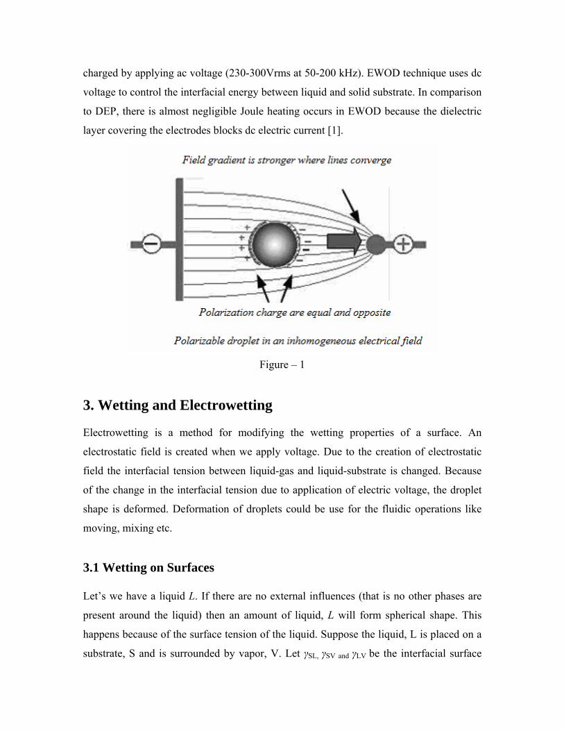
charged by applying ac voltage (230-300Vrms at 50-200 kHz). EWOD technique uses dc
voltage to control the interfacial energy between liquid and solid substrate. In comparison
to DEP, there is almost negligible Joule heating occurs in EWOD because the dielectric
layer covering the electrodes blocks dc electric current [1].
Figure – 1
3. Wetting and Electrowetting Electrowetting is a method for modifying the wetting properties of a surface. An
electrostatic field is created when we apply voltage. Due to the creation of electrostatic
field the interfacial tension between liquid-gas and liquid-substrate is changed. Because
of the change in the interfacial tension due to application of electric voltage, the droplet
shape is deformed. Deformation of droplets could be use for the fluidic operations like
moving, mixing etc.
3.1 Wetting on Surfaces Let’s we have a liquid L. If there are no external influences (that is no other phases are
present around the liquid) then an amount of liquid, L will form spherical shape. This
happens because of the surface tension of the liquid. Suppose the liquid, L is placed on a
substrate, S and is surrounded by vapor, V. Let γSL, γSV and γLV be the interfacial surface
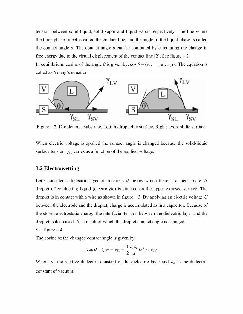
tension between solid-liquid, solid-vapor and liquid vapor respectively. The line where
the three phases meet is called the contact line, and the angle of the liquid phase is called
the contact angle θ. The contact angle θ can be computed by calculating the change in
free energy due to the virtual displacement of the contact line [2]. See figure – 2.
In equilibrium, cosine of the angle θ is given by, cos θ = (γSV − γSL ) / γLV. The equation is
called as Young’s equation.
Figure – 2: Droplet on a substrate. Left: hydrophobic surface. Right: hydrophilic surface.
When electric voltage is applied the contact angle is changed because the solid-liquid
surface tension, γSL varies as a function of the applied voltage.
3.2 Electrowetting Let’s consider a dielectric layer of thickness d, below which there is a metal plate. A
droplet of conducting liquid (electrolyte) is situated on the upper exposed surface. The
droplet is in contact with a wire as shown in figure – 3. By applying an electric voltage U
between the electrode and the droplet, charge is accumulated as in a capacitor. Because of
the stored electrostatic energy, the interfacial tension between the dielectric layer and the
droplet is decreased. As a result of which the droplet contact angle is changed.
See figure – 4.
The cosine of the changed contact angle is given by,
cos θ = (γSV − γSL + 2012
r Ud
ε ε ) / γLV
Where rε the relative dielectric constant of the dielectric layer and 0ε is the dielectric
constant of vacuum.
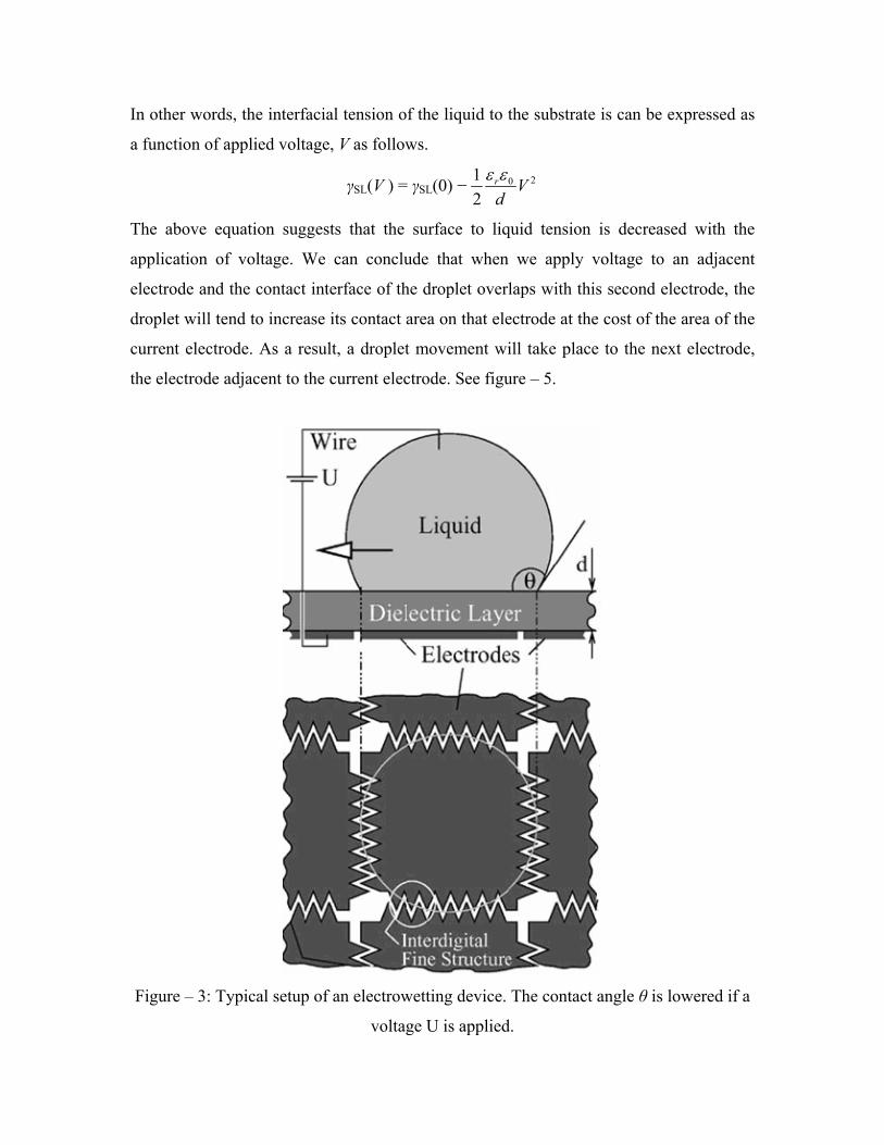
In other words, the interfacial tension of the liquid to the substrate is can be expressed as
a function of applied voltage, V as follows.
γSL(V ) = γSL(0) − 2012
r Vd
ε ε
The above equation suggests that the surface to liquid tension is decreased with the
application of voltage. We can conclude that when we apply voltage to an adjacent
electrode and the contact interface of the droplet overlaps with this second electrode, the
droplet will tend to increase its contact area on that electrode at the cost of the area of the
current electrode. As a result, a droplet movement will take place to the next electrode,
the electrode adjacent to the current electrode. See figure – 5.
Figure – 3: Typical setup of an electrowetting device. The contact angle θ is lowered if a
voltage U is applied.
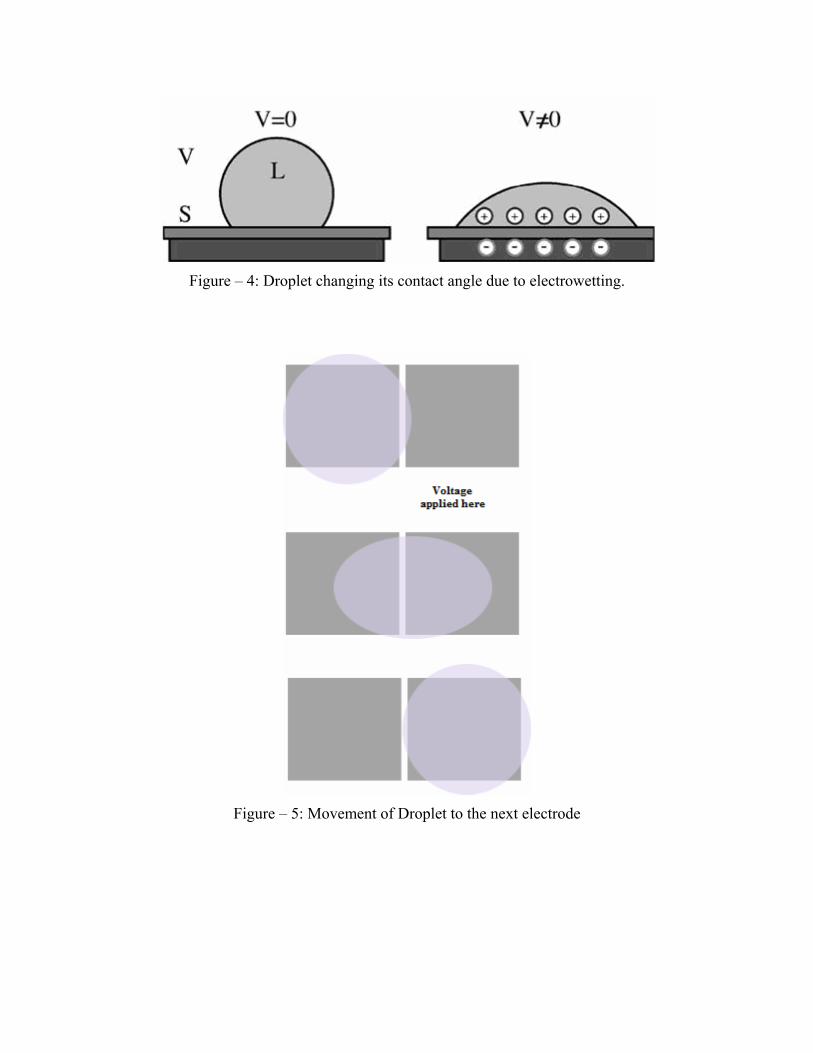
Figure – 4: Droplet changing its contact angle due to electrowetting.
Figure – 5: Movement of Droplet to the next electrode
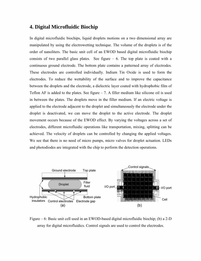
4. Digital Microfluidic Biochip In digital microfluidic biochips, liquid droplets motions on a two dimensional array are
manipulated by using the electrowetting technique. The volume of the droplets is of the
order of nanoliters. The basic unit cell of an EWOD based digital microfluidic biochip
consists of two parallel glass plates. See figure – 6. The top plate is coated with a
continuous ground electrode. The bottom plate contains a patterned array of electrodes.
These electrodes are controlled individually. Indium Tin Oxide is used to form the
electrodes. To reduce the wettability of the surface and to improve the capacitance
between the droplets and the electrode, a dielectric layer coated with hydrophobic film of
Teflon AF is added to the plates. See figure – 7. A filler medium like silicone oil is used
in between the plates. The droplets move in the filler medium. If an electric voltage is
applied to the electrode adjacent to the droplet and simultaneously the electrode under the
droplet is deactivated, we can move the droplet to the active electrode. The droplet
movement occurs because of the EWOD effect. By varying the voltages across a set of
electrodes, different microfluidic operations like transportation, mixing, splitting can be
achieved. The velocity of droplets can be controlled by changing the applied voltages.
We see that there is no need of micro pumps, micro valves for droplet actuation. LEDs
and photodiodes are integrated with the chip to perform the detection operations.
Figure – 6: Basic unit cell used in an EWOD-based digital microfluidic biochip; (b) a 2-D
array for digital microfluidics. Control signals are used to control the electrodes.
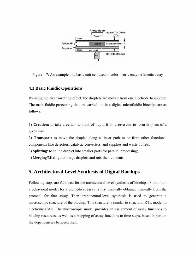
Figure – 7: An example of a basic unit cell used in colorimetric enzyme-kinetic assay
4.1 Basic Fluidic Operations By using the electrowetting effect, the droplets are moved from one electrode to another.
The main fluidic processing that are carried out in a digital microfluidic biochips are as
follows:
1) Creation: to take a certain amount of liquid from a reservoir to form droplets of a
given size.
2) Transport: to move the droplet along a linear path to or from other functional
components like detectors, catalytic converters, and supplies and waste outlets;
3) Splitting: to split a droplet into smaller parts for parallel processing;
4) Merging/Mixing: to merge droplets and mix their contents.
5. Architectural Level Synthesis of Digital Biochips Following steps are followed for the architectural level synthesis of biochips. First of all,
a behavioral model for a biomedical assay is first manually obtained manually from the
protocol for that assay. Then architectural-level synthesis is used to generate a
macroscopic structure of the biochip. This structure is similar to structural RTL model in
electronic CAD. The macroscopic model provides an assignment of assay functions to
biochip resources, as well as a mapping of assay functions to time-steps, based in part on
the dependencies between them.

The architectural-level synthesis for microfluidics-based biochips can be viewed as the
problem of scheduling assay functions and binding them to a given number of resources
so as to maximize parallelism, thereby decreasing response time.
5.1 Sequencing Graph Model The sequencing graph model is a directed acyclic graph G (V, E) where V are the nodes
of the graph and E are the edges of the graph. Each node of the graph represents a
biomedical assay operation (like dispensing, mixing, detection, dilution etc.) and each
edge between nodes represents the dependencies between the operations. Let V1
represents operation1 and V2 represents operation2. If operation2 is dependent on
operation1 then we put a directed edge from V1 to V2. There are two nodes; a source node
and sink node which represent no operations. These nodes are NOP nodes. Each node is
associated with a weight which represents the time required for the completion of that
operation. The source and the sink nodes have zero weight.
Different types of assay operations are:
1. Input Operation: These operations consists of the generation of the droplets of
samples (Si, i =1. ..,m ) or reagents (Ri, i =1, ..., n) from the on-chip reservoir,
which are then dispensed into the microfluidic array. The assumption for this
operation is that the weights of the all input nodes have the same weight. That is
the time required for generating and dispensing of different types of samples and
reagents are same.
2. Mixing Operations: In order to perform the required enzymatic assay, droplets of
samples need to be mixed with droplets of reagents on the microfluidic array. The
assumption for this operation is that the mixing of a sample with different
reagents takes the same amount of time since the reagents are extremely diluted
by buffer fluids like water.
3. Detection Operations: After mixing, the results of biomedical assay are detected
using an integrated LED-photodiode setup. Here it is assumed that the detection
time is determined by the type of enzymatic assay operation.

4. Dilution Operation: Reagents are mixed with the buffer fluid to produce the
diluted reagents.
In the next segment multiplexed in-vitro diagnostics on human physiological fluids is
described and its sequencing graph is shown in figure – 8 [5].
5.1.1 Sequencing Graph for Multiplexed in-vitro Diagnostics on Human Physiological fluid Many medical diagnoses require the measurement of glucose, lactate, pyruvate etc. in
human physiological fluids like urine, plasma and serum. The in-vitro diagnostics is of
great importance for metabolic disorders. Different colorimetric enzyme-kinetic assays
like glucose assay, pyruvate assay have been separately demonstrated by using
microfluidic biochips. By using the similar enzymatic reactions and different reagents,
these assay operations can be integrated to form a multiplexed in-vitro diagnostics on
different human physiological fluids, which can be performed concurrently on a
microfluidic biochip.
Figure – 8: Sequencing graph model of assay example
[3] describes an Integer Linear Programming model and heuristics approach for obtaining
an optimal schedule under resource constraints of the assay operations.

6. Module Placement Placement is one of the important physical design problems for digital microfluidics-
based biochips. After the schedule of bioassay operation, a set of microfluidic modules,
and the binding of bioassay operations to modules is obtained from architectural
synthesis, module placement determines the geometrical locations of each module on the
microfluidic array in order to optimize some design metrics.
The most promising advantage of digital microfluidic biochip is about its dynamic re-
configurability during the run time. That is these chips allow he placement of different
modules on the same location during different time intervals. Thus, the placement of
modules on the microfluidic array can be modeled as a 3-D packing problem. Each
microfluidic module is represented by a 3-D box, the base of which denotes the
rectangular area of the module and the height denotes the time-span of its operation. The
microfluidic biochip placement can now be viewed as the problem of packing these
boxes to minimize the total base area, while avoiding overlaps.
Figure – 9: Reduction of 3D problem to a modified 2D problem
This 3D packing problem can be reduced to a modified 2D placement problem as
follows. The starting time of each module operation is known from the schedule obtained
from architectural level synthesis. Therefore we know the position of modules in the time
axis. The horizontal cuts with the 3-D boxes correspond to the configurations of the
microfluidic array at different point in time.
For example, in Figure 9, the cut t = t1 corresponds to a 2-D placement shown in Figure
9(b), and the cut t = t2 corresponds to another configuration in Figure 9(c). The
configurations of the microfluidic array during different time intervals can be combined
together to form a modified 2-D placement shown in Figure 9(c).
Now several cutting planes (2D configurations) are generated at time t = Si. The Si
represents the starting time of module i’s operation. The placement of modules present on
each cutting planes can be solved as 2D packing problem. Thus, instead of a 3-D packing
problem, we only need to consider a modified 2-D placement consisting of several 2-D
configurations in different time spans.
[4] presents a simulated annealing based algorithm for solving module placement
problem. In addition, it also takes the fault tolerance of the chip into account while
finding the module placement.
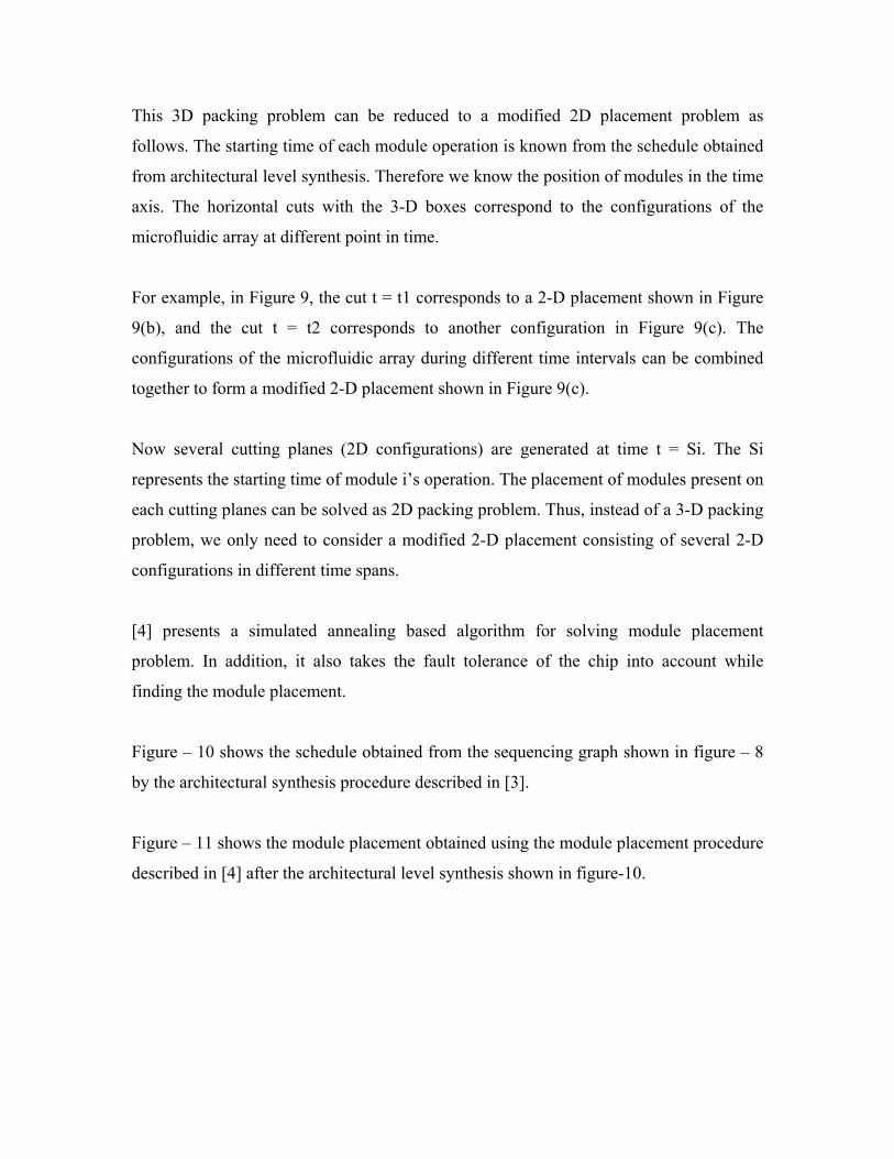
Figure – 10 shows the schedule obtained from the sequencing graph shown in figure – 8
by the architectural synthesis procedure described in [3].
Figure – 11 shows the module placement obtained using the module placement procedure
described in [4] after the architectural level synthesis shown in figure-10.
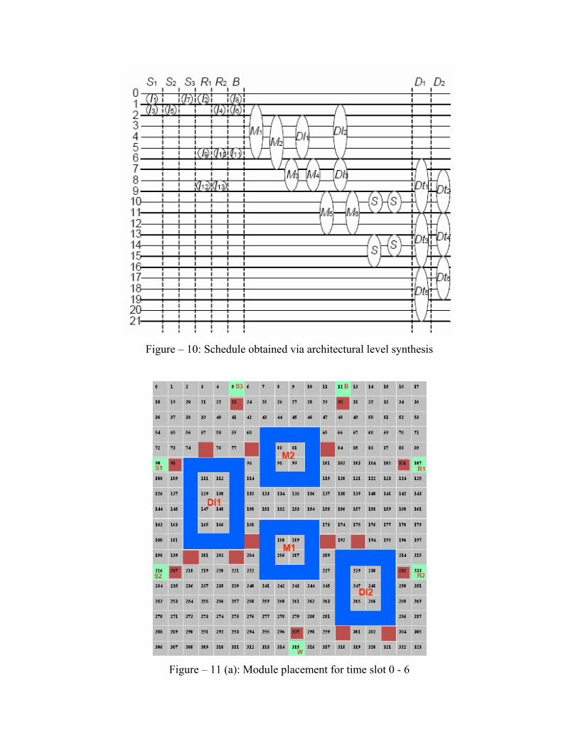
Figure – 10: Schedule obtained via architectural level synthesis
Figure – 11 (a): Module placement for time slot 0 - 6

Figure – 11 (b): Module placement for time slot 6 – 9
Figure – 11 (c): Module placement for time slot > 9
7. The Droplet Routing 7.1. Objective function The objective of routing problem in microfluidic chips is to find out the path from one
module to the other using minimum possible basic cells. To accommodate fault tolerance,
i.e. when a primary cell fails to perform bioassay, spare cells are used as primary cells to
complete the assay operations. So if the number of cells used during routing is minimized
(i.e., droplet route length is minimized) we can be left with more spare cells to
accommodate fault tolerance. This is very important in safety critical systems, which are
governed by biochips, because these types of systems require high fault tolerance.
For the routing purpose we require the net informations. A net is defined as the droplet
route between pins of different modules. The fluidic ports on the boundary of each
module represent pins of that module. The pin assignment is done during the placement
phase. So once we get the information about nets we can apply the routing algorithm to
find out the droplet routes. In the case of digital microfluidic biochips we can model nets
as 2-pin nets or 3-pin nets. A fluidic route on which a single droplet is transported
between pins of two different modules can be modeled as 2-pin net. To carry out mixing
operation two droplets traverse towards a mixer module. During the traversal, these
droplets can merge with each other. we need to model such fluidic routes using 3- pin
nets, instead of two individual 2-pin nets.
7.2. Fluidic Constraints The accidental mixing of droplets during transportation is avoided except when the two
droplets are required to merge during mixing operations. So it is always required to keep
a safe distance between any two droplets on the chip. Also during the routing of droplets
it should always be ascertained that there is no conflict between droplet routes and assay
operations. Thus, droplet routing is needed to be isolated from active modules. For the
isolation from modules, each module is associated with a segregation region which is
wrapped around the functional regions of the modules.
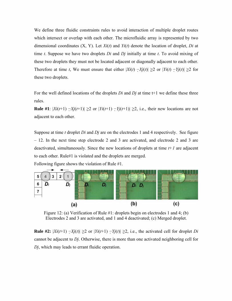
We define three fluidic constraints rules to avoid interaction of multiple droplet routes
which intersect or overlap with each other. The microfluidic array is represented by two
dimensional coordinates (X, Y). Let Xi(t) and Yi(t) denote the location of droplet, Di at
time t. Suppose we have two droplets Di and Dj initially at time t. To avoid mixing of
these two droplets they must not be located adjacent or diagonally adjacent to each other.
Therefore at time t, We must ensure that either |Xi(t) −Xj(t)| ≥2 or |Yi(t) −Yj(t)| ≥2 for
these two droplets.
For the well defined locations of the droplets Di and Dj at time t+1 we define these three
rules.
Rule #1: |Xi(t+1) −Xj(t+1)| ≥2 or |Yi(t+1) −Yj(t+1)| ≥2, i.e., their new locations are not
adjacent to each other.
Suppose at time t droplet Di and Dj are on the electrodes 1 and 4 respectively. See figure
– 12. In the next time step electrode 2 and 3 are activated, and electrode 2 and 3 are
deactivated, simultaneously. Since the new locations of droplets at time t+1 are adjacent
to each other. Rule#1 is violated and the droplets are merged.
Following figure shows the violation of Rule #1.
Figure 12: (a) Verification of Rule #1: droplets begin on electrodes 1 and 4; (b) Electrodes 2 and 3 are activated, and 1 and 4 deactivated; (c) Merged droplet.
Rule #2: |Xi(t+1) −Xj(t)| ≥2 or |Yi(t+1) −Yj(t)| ≥2, i.e., the activated cell for droplet Di
cannot be adjacent to Dj. Otherwise, there is more than one activated neighboring cell for
Dj, which may leads to errant fluidic operation.

Rule #3: |Xi(t) −Xj(t+1)| ≥2 or |Yi(t) −Yj(t+1)| ≥2. Similar to Rule #2.
Note that Rule #1 can be considered as the static fluidic constraint, whereas Rule #2 and
Rule #3 are dynamic fluidic constraints.
Suppose initially droplets Di and Dj are on the electrodes 4 and 7. See figure – 13. In the
next time step electrodes 3 and 6 are activated, and 4 and 7 deactivated. We can see
Rule#3 is violated for droplet Di because it is adjacent to electrode 3 and also diagonally
adjacent to electrode 6.
Following figure shows violation of Rule #3. The rule is violated for droplet Di
Figure - 13: (a) Experimental verification of Rule #3: droplets begin on electrodes 4 and
7; (b) Electrodes 3 and 6 are activated, and 4 and 7 deactivated; (c) Merged droplet.
Moreover, these fluidic constraint rules are not only used for rule checking, but they can
also provide guidelines to modify droplet motion (e.g., force some droplets to remain
stationary in a time-slot) to avoid constraint violation if necessary; the details of such a
strategy are discussed in the section 8.3. 7.3. Timing Constraints There is one more important constraint on droplet routing. This constraint is about upper
limit on droplet transportation time between two modules. In [3], which describes about
architectural level synthesis of microfluidic biochip, it is assumed that since the droplet
movement is very fast compared to assay operation (mixing, detection, etc.) times the
droplet routing time is not considered while computing a scheduling for assay operations.
So it must be ensured that the droplet routing delay does not exceed beyond a particular
value say, 10% of a time slot used in the scheduling. Otherwise, the schedule obtained
would no longer be valid. This timing constraint is similar to the interconnect delay
constraints in VLSI routing that require each wire net (or critical path) to meet its timing
budget. Note that since a droplet may be held at a location in some time slots during its
route, the delay for each droplet route is not identical to the route length. The delay for a
droplet route therefore consists of the transport time as well as the idle time.
7.4. Problem decomposition Digital microfluidics based biochips are dynamically reconfigurable. So during the
module placement phase a series of 2-D placement configurations are obtained in
different time spans instead of a single 2-D placement in classical VLSI design [4].
In this way, the droplet routing problem is divided into a series of sub-problems. In each
sub-problem, the nets to be routed between different modules are determined first. Only
the microfluidic modules that are active during this time interval are considered as
obstacles in droplet routing. Next suitable routes for these nets are found. These sub-
problems are solved sequentially to obtain a complete solution for droplet routing.
8. Routing Method The inputs to the algorithm are a list of nets to be routed in each sub-problem. The
droplet routing algorithm consists of two stages.
8.1. Phase I: M-shortest routes In this phase, M alternative routes for each net are generated. The maze routing algorithm
can be applied to find out the routes.
8.1.1. Two-pin nets. The shortest route problem for 2-pin nets is equivalent to the single-pair shortest path
problem.
8.1.2. Three-pin nets We use 3-pin nets to model the routes along which two droplets are transported towards a
microfluidic module (e.g., a mixer); the droplets can mix together during their
transportation. The shortest-route problem for such nets is equivalent to the Steiner
Minimum Tree (SMT) problem.
Out of these M alternative routes those which fail timing delay constraint check (TDCC)
are discarded.
8.2. Phase II: random selection In the second phase of the algorithm, a single route from the Mi alternatives for each net
i is selected, where i∈ {1, 2, …N} and N is the number of nets. Note that Mi ≤M since
some routes that violate the timing constraint have already been eliminated. A random
selection approach is then used to select ik for each net i, where ik represents the k-th
alternative route for net i, and k ∈{1, 2, …, Mi}. A desirable feature of this random
method is that it avoids the net-routing order dependence problem.
The set of selected routes are evaluated on the basis of number of cells used in routing.
The cost function C = number of cells used in routing. Then once again we check the
constraint upon selected routes. If it fails fluid constraint rule check (FCRC) (including
droplet motion modification discussed in Section 8.3) or TDCC, we assign a large
penalty value Pt to this set of routes, so that these routes are not selected. Otherwise, we
set Pt = 0 for those that satisfy all constraints.
After an adequate number of random selection runs, we select the set of routes with the
minimum cost value C and Pt = 0 as the output of the routing algorithm.
8.3. FCRC and droplet motion modification Assume that two droplet routes (i.e., Pi and Pj) have been obtained. To adhere to fluidic
constraint rules, we need to check these two droplets Di and Dj in each time slot. Even if
a rule violation is found, the droplet motion can still be modified (i.e., force a droplet to
stay in the current cell instead of moving) to override the violation; see Table 1. If the
modification fails (as in last the row of Table 1), the corresponding routing paths are no
more feasible.
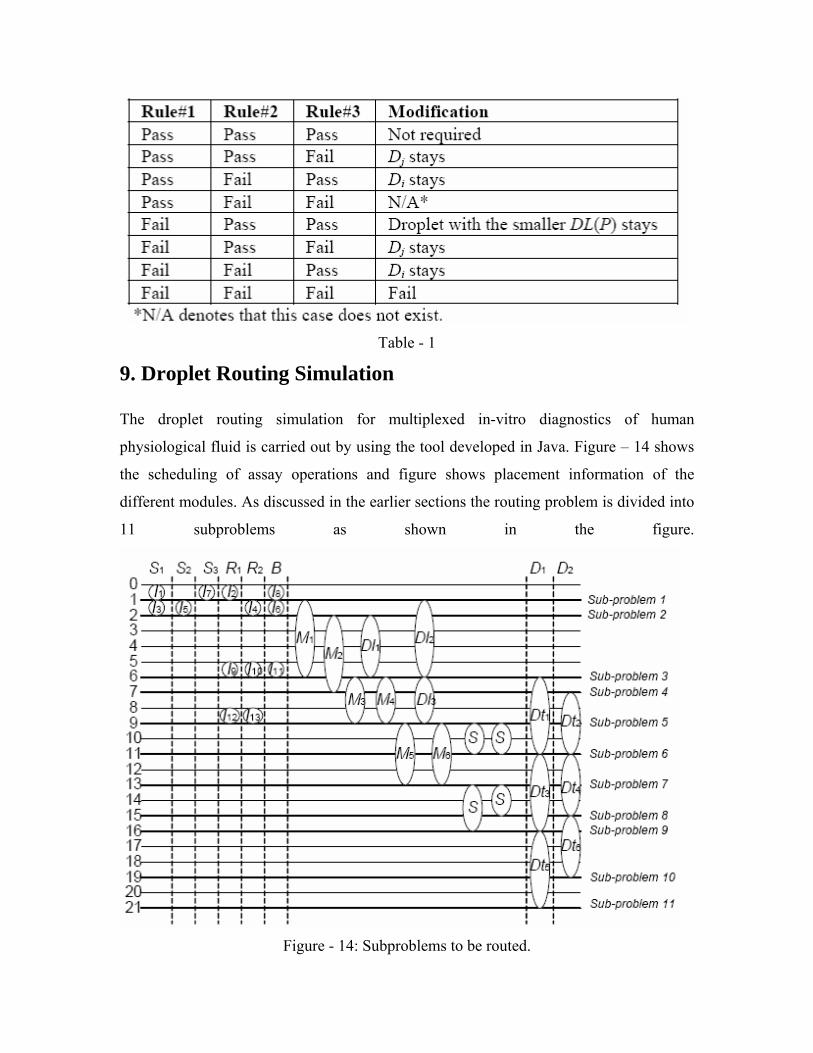
Table - 1
9. Droplet Routing Simulation The droplet routing simulation for multiplexed in-vitro diagnostics of human
physiological fluid is carried out by using the tool developed in Java. Figure – 14 shows
the scheduling of assay operations and figure shows placement information of the
different modules. As discussed in the earlier sections the routing problem is divided into
11 subproblems as shown in the figure.
Figure - 14: Subproblems to be routed.
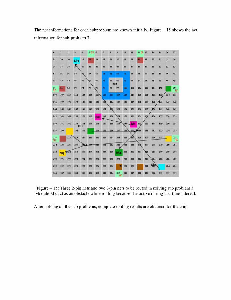
The net informations for each subproblem are known initially. Figure – 15 shows the net
information for sub-problem 3.
Figure – 15: Three 2-pin nets and two 3-pin nets to be routed in solving sub problem 3. Module M2 act as an obstacle while routing because it is active during that time interval.
After solving all the sub problems, complete routing results are obtained for the chip.
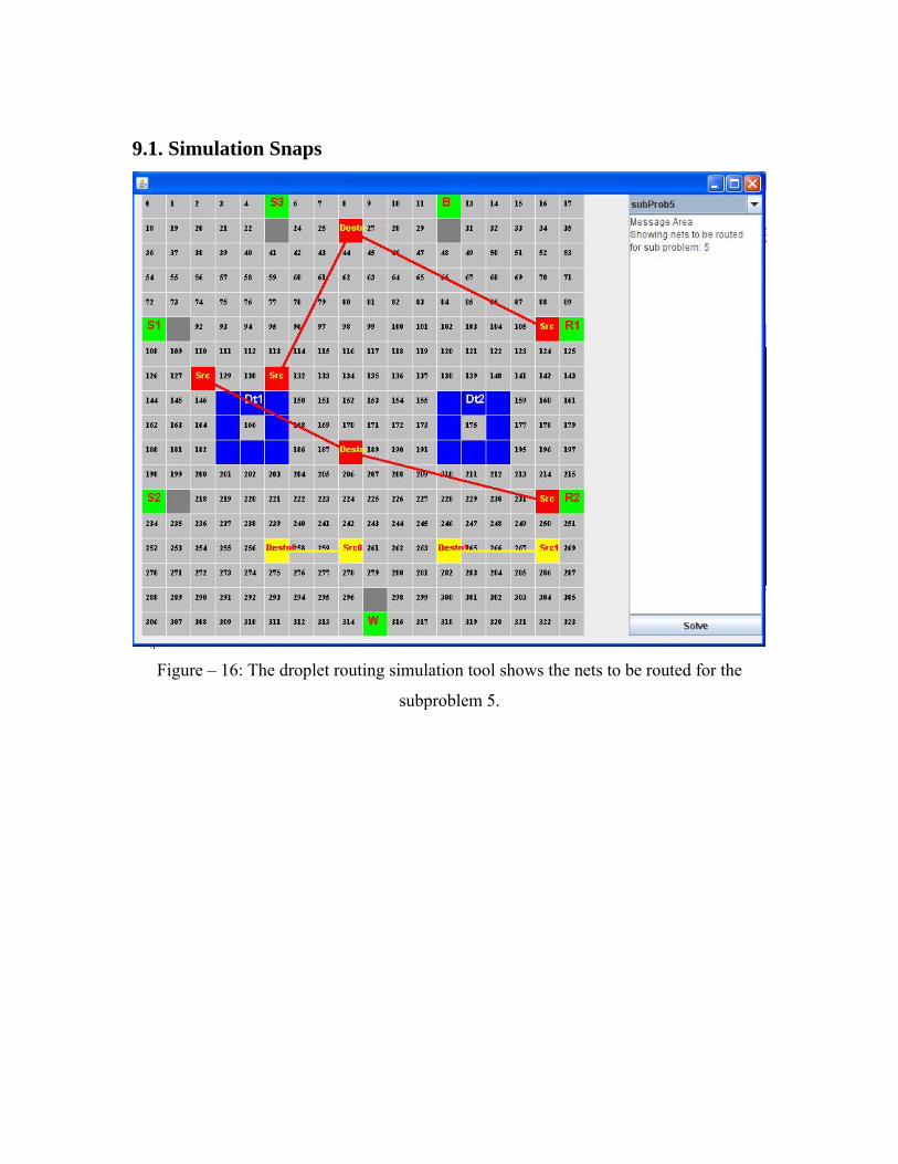
9.1. Simulation Snaps
Figure – 16: The droplet routing simulation tool shows the nets to be routed for the
subproblem 5.
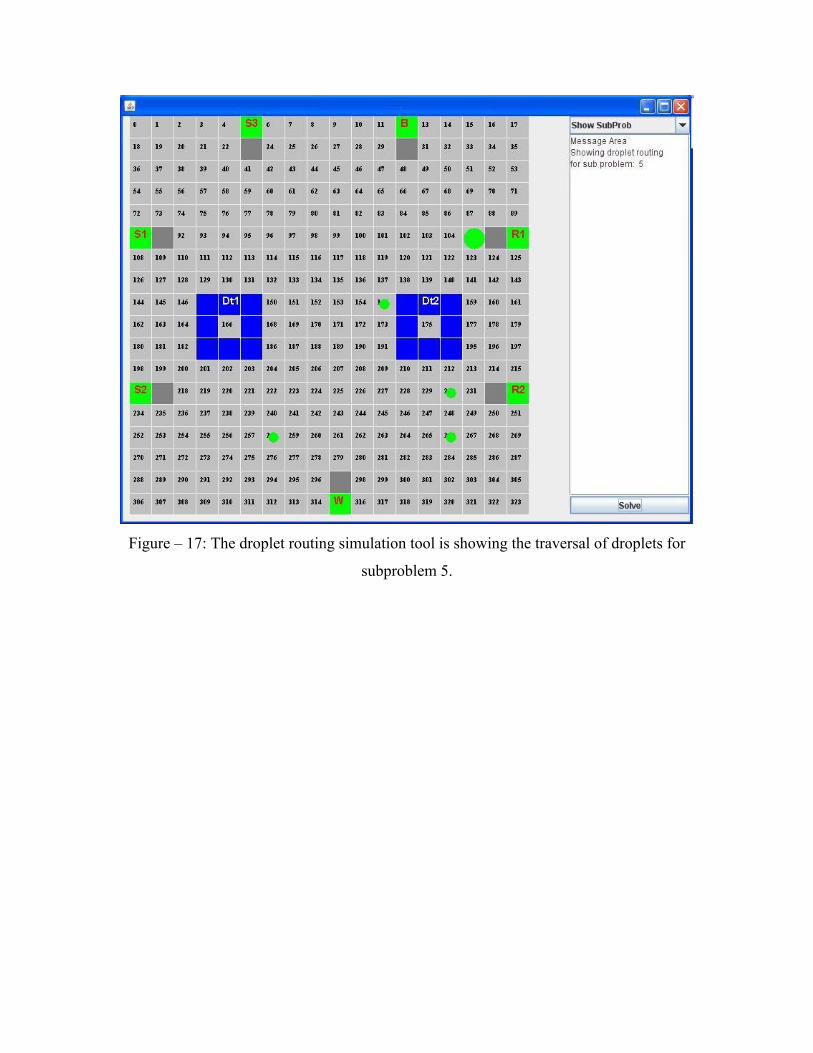
Figure – 17: The droplet routing simulation tool is showing the traversal of droplets for
subproblem 5.
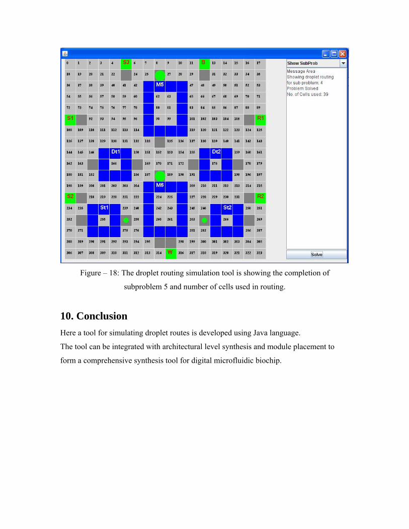
Figure – 18: The droplet routing simulation tool is showing the completion of
subproblem 5 and number of cells used in routing.
10. Conclusion Here a tool for simulating droplet routes is developed using Java language.
The tool can be integrated with architectural level synthesis and module placement to
form a comprehensive synthesis tool for digital microfluidic biochip.
11. References [1] Fei Su, Krishnendu Chakrabarty, Richard B. Fair.”Microfluidics-Based Biochips: Technology Issues, Implementation Platforms, and Design-Automation Challenges “ IEEE TRANSACTIONS ON COMPUTER-AIDED DESIGN OF INTEGRATED CIRCUITS AND SYSTEMS, VOL. 25, NO. 2, FEBRUARY 2006 [2] Jan Lienemann, Andreas Greiner, and Jan G. Korvink “Modeling, Simulation, and Optimization of Electrowetting” - IEEE TRANSACTIONS ON COMPUTER-AIDED DESIGN OF INTEGRATED CIRCUITS AND SYSTEMS, VOL. 25, NO. 2, FEBRUARY 2006. page 236 – 238. [3] F. Su and K. Chakrabarty, “Architectural-level synthesis of digital microfluidics-based biochips” [4] F. Su and K. Chakrabarty, “Design of fault-tolerant and dynamically-reconfigurable microfluidic biochips” [5] Fei Su, William Hwang and Krishnendu Chakrabarty, “Droplet Routing in the Synthesis of Digital Microfluidic Biochips.” [6] F. Su and, K. Chakrabarty et al. “Concurrent Testing of Digital Microfluidics-Based Biochips”, ACM Transactions on Design Automation of Electronic Systems, Vol. 11, No. 2, April 2006, pages 444 – 445.