dynamic interactions between interest-rate and credit...

Dynamic Interactions Between Interest-Rate and Credit Risk:Theory and Evidence on the Credit Default Swap Term Structure∗

REN-RAW CHEN1, XIAOLIN CHENG2, LIUREN WU3

1Graduate School of Business, Fordham University;2 Morgan Stanley;3Zicklin School of Business, Baruch

College, City University of New York

Abstract. This paper examines the interaction between default risk and interest-rate risk in determining the

term structure of credit default swap spreads at different industry sectors and credit rating classes. The paper

starts with a parsimonious three-factor interest-rate dynamic term structure and projects the credit spread at

each industry sector and rating class to these interest-rate factors while also allowing the projection residual

dynamics to depend on the level of the interest-rate factors. Estimation shows that credit risk exhibits

intricate dynamic interactions with the interest-rate factors.

JEL Classification:E43, G12, G13, C51.

Keywords:Credit default swap; credit risk; term structure; interest-rate risk; maximum likelihood estima-

tion.

∗We thank Bernard Dumas (the editor), an anonymous referee, Jennie Bai, Lasse Pedersen, Mike Long, Jiang Wang, and seminarparticipants at Rutgers University, Baruch College, Fitch, Moody’s KMV, and the 13th Annual Conference on Pacific BasinFinance,Economics, and Accounting at Rutgers for helpful comments.Send correspondence to Liuren Wu, Department of Economics andFinance, Zicklin School of Business, Baruch College, City University of New York, One Bernard Baruch Way, Box B10-225, NewYork, NY 10010, telephone: (646) 312-3509, fax: (646) 312-3451. E-mail: [email protected].

1

1. Introduction

It is important to understand how credit risk interacts withinterest-rate risk in determining the term struc-

ture of credit spreads on different reference entities. Nevertheless, limited data availability has severely

hindered the understanding. Since defaults are rare eventsthat often lead to termination or restructuring of

the underlying reference entity, researchers need to rely heavily on cross-sectional averaging across different

entities over a long history to obtain any reasonable estimates of statistical default probabilities. Although

corporate bond prices contain useful information on the default probability and the pricing of credit risk,

the information is often mingled with the pricing of interest-rate risk and other factors such as liquidity and

tax.1

The development in the credit derivatives market provides an excellent opportunity for a better under-

standing of the dynamics and pricing of credit risk, its interactions with interest-rate risks, and their impacts

on the term structure of credit spreads. The most widely traded credit derivative is in the form of credit

default swap (CDS), an over-the-counter contract that provides protection against credit risk. The protection

buyer pays a fixed premium, often termed as the “CDS spread,” to the seller for a period of time. If a pre-

specified credit event occurs, the protection buyer stops the premium payment and receives compensation

from the protection seller. A credit event can be the bankruptcy of the reference entity, or default of a bond

or other debt issued by the reference entity. If no credit event occurs during the term of the swap, the pro-

tection buyer continues to pay the premium until maturity. The CDS spreads are commonly set at inception

to match the present values of the credit protection and premium payment so that no upfront payments are

necessary.2

With a large data set on CDS spread quotes, this paper performs a joint analysis on the term structure

of interest rates and credit spreads, with a focus on the dynamic interactions between the two sources of

risk. The data set includes daily CDS spread quotes on hundreds of corporate companies and across six

fixed maturities from one to ten years for each company. We classify the reference companies along two

dimensions: (i) industry sectors and (ii) credit ratings. We also download from Bloomberg the eurodollar

libor and swap rates of matching maturities and sample periods. Through model development and estima-

tion, we address the following fundamental questions regarding credit risk and its dynamic interactions with

1Many researchers strive to identify and distinguish the different components of corporate bond yields. Prominent examplesinclude Fisher (1959), Jones, Mason, and Rosenfeld (1984),Longstaff and Schwartz (1995), Duffie and Singleton (1997),Duf-fee (1999), Elton, Gruber, Agrawal, and Mann (2001), Pierre, Goldstein, and Martin (2001), Delianedis and Geske (2001), Liu,Longstaff, and Mandell (2006), Eom, Helwege, and Huang (2004), Huang and Huang (2003), Collin-Dufresne, Goldstein, andHelwege (2003), Ericsson and Renault (2006), and Longstaff, Mithal, and Neis (2005).

2The CDS market is undergoing structural and contractual reforms. To reduce counterparty risk, the market is moving towardcentral clearing. To facilitate netting, the market is alsomoving toward contract specifications with upfront payments and fixedpremium coupons of either 100 or 500 basis points. The data wehave are CDS spreads that result in zero upfront payments.

1

interest-rate risk:

• How many factors govern the term structure of credit spreads?

• How do the credit-risk factors interact with interest-ratefactors?

• How do the credit-risk dynamics and pricing differ across industry sectors and credit rating classes?

To address these questions, we develop a class of dynamic term structure models of interest-rate risk and

credit risk. First, we model the term structure of the benchmark libor and swap rates using three interest-

rate factors. Second, we assume that the default arrival intensities at each industry sector and credit rating

class are governed by either one or two dynamic factors. To capture the dynamic interactions between the

market-wide interest-rate risk and the specific credit riskat each industry sector and credit rating class, we

project the instantaneous credit spread of each classified group onto the interest-rate factors and further allow

the dynamics of the projection residuals to depend on the interest-rate factors. Through this specification,

changes in the interest-rate factors affect both contemporaneous and subsequent changes in the credit-risk

factors.

We estimate the models in a two-step sequential procedure. In the first step, we estimate the interest-

rate factor dynamics using the benchmark libor and swap rates. In the second step, we take the interest-

rate factors estimated from the first step as given, and estimate the credit-risk dynamics for each industry

sector and credit rating class using the average CDS spreadsfor that sector and rating class across different

maturities. At each step, we cast the models into a state-space form, obtain forecasts on the conditional mean

and variance of observed series using a nonlinear filtering technique, and build the likelihood function on

the forecasting errors of the observed series, assuming that the forecasting errors are normally distributed.

We estimate the model parameters by maximizing the likelihood functions.

Estimation shows that one credit-risk factor can price the moderate-maturity CDS spreads well, but the

performance deteriorates toward both ends of the credit spread curve. By contrast, two credit-risk factors can

price the whole term structure of credit spreads well. Our estimation also shows that firms in different indus-

try sectors and credit rating classes exhibit different credit-risk dynamics. Nevertheless, in all cases, credit

risk shows intricate dynamic interactions with the interest-rate factors. Interest-rate factors both impact the

credit spread contemporaneously, and affect subsequent changes in the credit-risk factors.

Our projection-based one-way interaction specification and our two-step sequential estimation procedure

provide a viable channel for analyzing the dynamic interactions between market-wide risk factors on the one

hand and industry/rating-specific risks on the other. To understand potential two-way interactions between

2

interest-rate risk and market-wide aggregate credit risk,we also consider an alternative two-way interactive

dynamics and identify the two-way interaction through joint estimation of the interest-rate and the market-

average CDS term structures. The joint estimation shows that the aggregate credit condition of the market

can also influence the monetary policy and hence the benchmark interest-rate curve. In particular, worsening

of the credit condition, represented by widening of averagecredit spreads, especially at long maturities,

tends to lead to future easing in monetary policy and accordingly lowering of the current forward interest-

rate curve. On the other hand, positive shocks to the short-term interest rate narrow the credit spread at

long maturities, whereas positive shocks to long-term interest rates widen the credit spreads. These results

highlight the intricate interactions between the two markets.

Understanding the dynamic interactions between interest rates and credit spreads has been a perennial

topic in the literature as it has important implications forcredit risk modeling. Early studies have often

identified a negative relation between credit spreads and short-term interest rates (Duffee (1998)). To be

consistent with this finding, many studies, e.g., Feldhutter and Lando (2008), Fruhwirth, Schneider, and

Sogner (2010), and Driessen (2005), directly incorporatea negative loading of the instantaneous interest rate

into the credit spread specification.3 Compared to such practices, we explicitly recognize the fact that the

instantaneous interest rate itself is driven by multiple risk factors, and that these different factors may have

different impacts on the credit spreads (Wu and Zhang (2008)). Accordingly, we allow the instantaneous

interest rate and credit spreads to depend on a common set of interest-rate factors with their different loadings

directly estimated from the term structure of libor/swap rates and CDS spreads. We further allow the credit-

risk factors to interact dynamically with the benchmark interest-rate factors. Thus, our modeling of the

interactions between interest rates and credit spreads goes far beyond what has been done in the literature.

Our work constitutes the first comprehensive analysis of thejoint term structure of interest rates and

credit spreads using the CDS data. In other related studies,Skinner and Diaz (2003) analyze CDS prices

from September 1997 to February 1999 for 31 CDS contracts. They compare the pricing results of the Duffie

and Singleton (1999) and Jarrow and Turnbull (1995) models.Blanco, Brennan, and Marsh (2005) compare

the CDS spreads with credit spreads derived from corporate bond yields and find that overall the two sources

of spreads match each other well. When the two sources of spreads deviate from each other, they find that

CDS spreads have a clear lead in price discovery. Longstaff,Mithal, and Neis (2005) regard the CDS spreads

as purely due to credit risk and use the CDS spreads as a benchmark to identify the liquidity component of

3In proposing models for pricing interest-rate derivatives, Brigo and Alfonsi (2005) allow instantaneous correlationbetween thetwo Brownian motions driving the interest rate and the default arrival rate, and analyze numerically the effect of this correlation oncalibration and pricing. Schneider, Sogner, and Veza (2010) analyze the loss given default and jumps in default risk using corporateCDS data, but they assume independence between interest rate and default risk.

3

corporate yield spreads. They find that a major portion of thecorporate spread is due to credit risk. Hull,

Predescu, and White (2004) examine the relation between theCDS spreads and announcements by rating

agencies. Zhang (2008) uses sovereign CDS to study the case of Argentine default. Carr and Wu (2007)

model and estimate the dynamic interaction between sovereign CDS spreads and currency options. Cremers,

Driessen, Maenhout, and Weinbaum (2008) and Carr and Wu (2010, 2011) analyze the link between CDS

spreads and stock option prices.

The remainder of the paper is organized as follows. Section 2describes the data set and documents the

stylized evidence on the CDS spreads that motivates our theoretical efforts in Section 3, where we develop

the dynamic term structure models that allow intricate dynamic interactions between interest-rate risk and

credit risk. Section 4 describes our model estimation strategy. Section 5 discusses the estimation results.

Section 6 explores potential two-way interactions betweeninterest rates and market-average CDS spreads.

Section 8 concludes.

2. Data and Evidence

We obtain daily CDS spread quotes from an investment bank at six fixed time-to-maturities at one, two,

three, five, seven, and ten years from May 21, 2003 to October 8, 2007, spanning 1,142 business days. For

each firm, the data set also contains an expected recovery rate estimate at each date. We obtain the credit

rating information on each reference company from Standard& Poors, and the sector information from

Reuters.

At each date, we divide the CDS data into four groups based on (i) two broad industry classifications:

financial and corporate, and (ii) two broad credit rating groups: A (including A+ and A-) and BBB (including

BBB+ and BBB-). Companies without credit rating information or with ratings above A or below BBB are

excluded. For each group and at each maturity, we compute a weighted average CDS value, where the

weight is computed based on the deviation of each quote from the median value. To reduce the impact of

potential outliers, we set the weight to zero when a quote is 1.28 standard deviations away from the median.

This criterion excludes about 10% of the quotes on each side of the spectrum. The particular choice of the

weighting function and the truncation criterion are chosenbased on the analysis of the data behavior and the

stability of the resulting series. The number of quotes included in each average varies from a minimum of

four quotes to a maximum of 299. The number of firms in our data set increases over time. Accordingly, the

number of quotes included in the average also increases overtime. The number of firms averages at 47 for

financial firms with A rating, 43 for financial firms with BBB rating, 106 for corporate with A rating, and

4

204 for corporate with BBB rating.

Figure 1 plots the time series of the average CDS spreads at each industry sector and credit rating class.

The six lines in each panel correspond to the six time series at different maturities, with the solid line

denoting the one-year CDS series, the dash-dotted line denoting the 10-year CDS series, and the dashed

lines for the intermediate maturities. In all four panels, the solid line for the one-year CDS series always

stays at the bottom of the six lines whereas the dash-dotted line for the 10-year CDS series always stays at

the top of the six lines, showing that the CDS term structure is always upward sloping during our sample

period. The time series in Figure 1 show stronger co-movements across different maturities within the same

panel (i.e., within the same industry sector and rating class) than co-movements across different panels.

[Figure 1 about here.]

Table I reports the summary statistics of the average CDS spreads under each industry sector and credit

rating classification. The mean spreads are higher at longermaturities for all groups, generating an upward-

sloping mean term structure. Within each industry sector and at each fixed maturity, the mean spreads are

higher for BBB firms than for A firms. Within each credit ratingclass, the mean spreads are slightly higher

for financial firms than for non-financial firms.

[Table I about here.]

The standard deviations of the spreads show an upward sloping term structure for the financial sector and

the A rating class, but the term structure is either downwardsloping or hump-shaped for other groups. The

skewness and excess kurtosis estimates are mostly small. The daily autocorrelation estimates are between

0.98 and 0.99, indicating that the CDS spreads are highly persistent. The last row in each panel reports the

summary statistics on the expected recovery rates, which average close to 40%, with small time variation.

To estimate the benchmark interest-rate dynamics, we obtain eurodollar libor and swap rates from

Bloomberg that match the maturity and sample period of the CDS data. Figure 2 plot the time series of

the interest-rate series, with the solid line denoting the 12-month libor, the dash-dotted line denoting the

10-year swap rate, and the dashed lines denoting swap rates with maturities from two to seven years. The

interest rates show a steeply upward sloping term structureat the beginning of the sample but the term struc-

ture becomes flat since 2006, with the 12-month libor being close to or even higher than the 10-year swap

rate.


5

Table II reports the summary statistics of the six interest-rate series. The interest rates average between

3.73% to 4.93%, with an average upward sloping term structure. The standard deviation estimates are

downward sloping from 1.6 for the 12-month libor to 0.45 for the 10-year swap rate. The skewness and

excess kurtosis estimates are small. The daily autocorrelation estimates range from 0.988 to 0.998, showing

extremely high persistence for these time series.

[Table II about here.]

3. Modeling the Dynamic Interactions between Interest Rateand Credit Risk

We value the CDS contracts under the framework of Duffie and Singleton (1999) and Duffie, Pedersen, and

Singleton (2003). Following the current industry standard, we define the benchmark instantaneous interest

ratert based on the eurodollar libor and swap rates.4 Libor and swap rates contain a credit risk component.

Using them as benchmarks, the estimated credit risk from CDSquotes can be regarded as relative credit

risk.

Let (Ω,F ,(F t)t≥0,Q) be a complete stochastic basis andQ be a risk-neutral probability measure, under

which the time-t fair value of a benchmark zero-coupon bond with maturityτ relates to the instantaneous

benchmark interest rate by,

P(t,τ) = Et

[

exp

(

−∫ t+τ

trudu

)]

, (1)

whereEt [·] denotes the expectation operator under the risk-neutral measureQ conditional on the time-t

filtration F t .

To value a CDS contract, letλit to denote the intensity of a Poisson process that governs thedefault of

a reference entityi. By modeling the dynamics of the Poisson intensitiesλi and their dynamic interactions

with the benchmark interest rates, we determine the term structure of the CDS spreads for entityi. Let

Si(t,τ) denote the premium rate that a protection buyer should pay onreference entityi for a maturity of

τ years to make the CDS contract worth zero at timet. Under the simplifying assumption of continuous

payment, the time-t present value of the premium leg of the contract is given by,

Premium(t,τ) = Et

[

Si(t,τ)∫ τ

0exp

(

−∫ t+s

t(ru+λi

u)du

)

ds

]

, (2)

4Historically, researchers often use Treasury yields to define the instantaneous interest rate and the benchmark yield curve.Houweling and Vorst (2005) perform daily calibration of reduced-form models using credit default swap spreads and find thateurodollar swap rates are better suited than the Treasury yields in defining the benchmark yield curve.

6

and the present value of the protection leg is,

Protection(t,τ) = Et

[

wi(t,τ)∫ τ

0λi

t+sexp

(

−∫ t+s

t(ru+λi

u)du

)

ds

]

, (3)

wherewi(t,τ) denotes the time-t expected loss rate upon default on reference entityi over the horizonτ. By

setting the present values of the two legs equal, one can solve for the CDS spread as,

Si(t,τ) =Et

[

wi(t,τ)∫ τ

0 λit+sexp

(

−∫ t+st (ru+λi

u)du)

ds]

Et[∫ τ

0 exp(

−∫ t+st (ru+λi

u)du)

ds] , (4)

which can be regarded as the weighted average of the expecteddefault loss. In model estimation, we

discretize the above equation according to quarterly premium payment intervals.

Under this framework, the benchmark libor and swap rate curve is determined by the dynamics of the

instantaneous benchmark interest rater. The CDS spreads of a certain reference entity are determined by

the joint dynamics of the instantaneous interest rater and the default arrival rateλi . We specify the two sets

of dynamics in the following subsections.

3.1. BENCHMARK INTEREST-RATE DYNAMICS AND THE TERM STRUCTURE

To enhance model identification, we model the benchmark instantaneous interest-rate dynamics with a par-

simonious dimension-invariant cascade structure developed by Calvet, Fisher, and Wu (2010). We apply a

three-factor structure and specify the factor dynamics under the statistical measureP as,

dx1,t = κrs2κ (x2,t −x1,t)dt+σrdW1

t ,

dx2,t = κrsκ (x3,t −x2,t)dt+σrdW2t ,

dx3,t = κr (θr −x3,t)dt+σrdW3t .

(5)

We set the instantaneous interest rate to the highest frequency componentrt = x1,t , which mean reverts to

a lower frequency stochastic factorx2,t , which mean revert to an even lower frequency factorx3,t , which

reverts to a constant meanθr . The cascade structure naturally ranks the three interest-rate factors in terms of

their relative frequency, which is distributed according to a power law scaling on the mean-reversion speeds,

with sκ > 1 denoting the scaling coefficient. For parsimony, we followCalvet, Fisher, and Wu (2010) in

assuming independent and identically distributed factor innovations and using one parameterσr to capture

the instantaneous risk level, withE[dWit dW j

t ] = 0 for all i 6= j. We further assume that the market prices on

all three Brownian risks are identical and constant atγr . With these assumptions, the interest rate statistical

dynamics and term structure behavior are captured by merelyfive free parameters(κr ,sκ,θr ,σr ,γr).

7

In matrix notation, we can write the statistical dynamics for the interest-rate factorsXt ≡ [x1,t ,x2,t ,x3,t ]⊤

as,

dXt = κX (θr −Xt)dt+σrdWt , (6)

where the mean-reversion matrix is block diagonal,

κX =

κrs2κ −κrs2

κ 0

0 κrsκ −κrsκ

0 0 κr

, (7)

and all three factors have the same long-run meanθr . Given the constant market price assumption, the factor

dynamics under the risk-neutral measureQ are given by,

dXt = (CX −κXXt)dt+σrdWQt , (8)

where the mean-reversion matrix remains the same and the constant vectorCX is given by,

CX =[

−γrσr ,−γrσr ,κrθr − γrσ2r

]⊤. (9)

Under the above specifications, the time-t model value of the zero-coupon bond with time-to-maturityτ

is exponential affine in the current level of the state vector, Xt ,

P(Xt ,τ) = exp(

−a(τ)−b(τ)⊤Xt

)

, (10)

where the coefficients solve the ordinary differential equations,

b′ (τ) = br −κ⊤Xb(τ) , (11)

a′ (τ) = b(τ)⊤CX − 12

b(τ)⊤b(τ)σ2r , (12)

starting atb(τ) = 0 anda(τ) = 0, with br = [1,0,0]⊤. The ordinary differential equations can be solved

analytically (Calvet, Fisher, and Wu (2010)).

Given the solutions to the zero-coupon bonds, the model values for the libor and swap rates can be

8

computed as,

LIBOR(Xt,τ) =100

τ

(

1P(Xt,τ)

−1

)

, SWAP(Xt ,τ) = 100h× 1−P(Xt,τ)∑hτ

i=1 P(Xt , i/h), (13)

whereτ denotes the time-to-maturity andh denotes the number of payments in each year for the swap

contract. The day-count convention for libor is actual/360, starting two business days forward. For the U.S.

dollar swap rates that we use, the number of payments is twiceper year,h= 2, and the day-count convention

is 30/360.

Historically, the spreads between libor and the corresponding overnight interest rate (OIS) swap rate are

negligible as they average just about 10 basis points. The industry standard is to build one integrated interest-

rate curve from quotes on all libor and swap rates. Quotes on eurodollar futures are sometimes also used to

smooth the curve at intermediate maturities. During the 2007 financial crisis, the libor-OIS spread widened

dramatically to as high as 3.5 percentage points. Swaps withdifferent floating leg libor references often

trade at significantly different levels, prompting the practice of building multiple interest-rate curves, with

each curve corresponding to one libor tenor (Mercurio (2010a,b)). In this paper, we retain the simplifying

assumption that there is one interest-rate curve underlying all libor and swap rates.

Our interest-rate dynamics specification belongs to the general three-factor Gaussian-affine class of dy-

namic term structure models, discussed more generally in Duffie and Kan (1996), Duffee (2002), and Dai

and Singleton (2000, 2002). Gaussin-affine models are very tractable and can readily be linked to vector

autoregressive (VAR) specifications in discrete time (e.g., Joslin, Singleton, and Zhu (2011)). We choose

to apply strong structures to the dynamics for several reasons. First, the cascade interest-rate dynamics

naturally rank the interest-rate factors according to their mean-reversion speeds, with the first factor cap-

turing the highest frequency shocks and the last factor capturing shocks of the lowest frequency. Factor

rotation is a common issue in general linear-Gaussian specifications, making the factor identification and

interpretation difficult. The cascade structure that we adopt completely removes factor rotation and greatly

enhances the economic interpretation of these factors. Second, the dimension-invariant assumptions allow

us to use merely five parameters to model the interest-rate dynamics regardless of how many factors we

incorporate into the system. The extreme parsimony of the specification allows us to identify the model

parameters with strong statistical significance. Identification is a strong concern when estimating dynamics

on highly persistent time series, such as interest rates andcredit spreads (Duffee and Stanton (2008)). The

parsimonious dimension-invariant structure provides a structural approach in mitigating the identification

issues, especially when one needs to estimate high-dimensional models. Third, empirical analysis in Calvet,

9

Fisher, and Wu (2010) shows that the interest-rate data support the power-law scaling assumption across

different frequencies. Thus, the specification achieves parsimony and dimension invariance while matching

the observed behaviors of the data.

In reality, the pricing performance of a term structure model is mainly dictated by the number of factors

than by the number of parameters. An ideal model should have as many factors as needed to match the data

behavior while using as few free parameters as possible to enhance identification. The cascade dimension-

invariant specification represents a new class of models that move toward this direction.

Empirically, Bikbov and Chernov (2004) show that all three-factor affine models generate similar per-

formance in fitting the interest-rate term structure. In theAppendix, we also estimate a general three-factor

Gaussian affine specification with 19 free parameters. The estimation results show that the pricing perfor-

mance of this general specification is similar to the pricingperformance of our parsimonious specification,

as both models generate near perfect fitting to the observed interest-rate term structure.

3.2. CREDIT RISK DYNAMICS AND THE TERM STRUCTURE OFCDS SPREADS

To model the default arrival rate underlying each industry sector and credit rating classi, we first project the

arrival rateλt onto the interest-rate factorsXt ,5

λt = β⊤Xt +yt , (14)

whereβ denotes the instantaneous response of the default arrival rate to the three interest-rate factors, andyt

denotes the projection residual, capturing the credit riskcomponent that is contemporaneously orthogonal

to the interest-rate factors.

Although yt is contemporaneously orthogonal to the interest-rate factors by projection principles, the

two can still interact dynamically. We consider a two-factor structure for the credit risk while allowing such

dynamic interactions with the interest-rate factors. Under the statistical measureP, we specify the credit-risk

factor dynamics as,

dy1,t = κy,1 (y2,t −y1,t)dt+∑3j=1κ j

yx,1 (x j+1,t −x j,t)dt+σydW4t ,

dy2,t = κy,2 (θy−y2,t)dt+∑3j=1κ j

yx,2 (x j+1,t −x j,t)dt+σydW5t , x4 = θr ,

(15)

where the credit risk follows a two-factor cascade structure asyt = y1,t mean reverts to a slower component

y2,t , which reverts to a constant meanθy, with κy,1 > κy,2. Furthermore, the three interest-rate factors enter

5When no confusion shall occur, we suppress the industry sector/rating class referencei to reduce notation clustering.

10

the drifts of the two credit-risk factors to capture the dynamic interactions, withκyx,1 capturing how the

deviation of each interest-rate factor from its lower-frequency trend predicts future movements in the first,

higher-frequency credit risk factoryt , andκyx,2 capturing the prediction of the three interest-rate factors on

the lower-frequency credit-risk factory2,t . For parsimony, we assume independent and identically distributed

credit risk Brownian innovations and useσy to capture the risk magnitude while extending the independence

assumptionE[dWit dW j

t ] = 0 for all i 6= j. We further assume constant and identical market price for the two

credit Brownian risksγy. Thus, under the risk-neutral measureQ, the drift of each of the two factors will be

adjusted by−γyσy.

Existing studies often capture the interaction between interest rates and credit spreads through a direct

loading of the instantaneous default rate on the instantaneous interest rate (e.g., Feldhutter and Lando (2008)

and Fruhwirth, Schneider, and Sogner (2010)),

λt = brt +yt , (16)

whereb is often set negative given the empirical evidence (Duffee (1998)). By contrast, our specification

in (14) recognizes the fact that different frequency components of the interest-rate movements can have

different impacts on the term structure of credit spreads. Furthermore, Equation (15) incorporates another

layer of dynamic interaction absent from existing specifications in the literature. Together, our specifications

allow the interest-rate factors to both impact the default arrival rate contemporaneously through the loading

coefficientsβ and affect subsequent changes in the credit-risk factors through the interaction coefficients

κyx. For model estimation, we consider both the two-factor specification in (15) and a one-factor special

case by settingy2,t = θy.

We can write the joint risk-neutral dynamics of the interest-rate and credit risk factors in matrix form as,

Zt ≡ x j,t3j=1,yk,t2

k=1,

dZt = (C−κZt)dt+√

ΣdWQt , (17)

where the constant vector is given byC = [C⊤X ,−γyσy,κy,2θy− γyσy]

⊤, the covariance matrixΣ is diagonal

with the first three diagonal elements beingσ2r and the remaining two diagonal elements beingσ2

y, and the

11

mean-reverting matrixκ is given by

κ =

κrs2κ −κs2

κ 0 0 0

0 κrsκ −κrsκ 0 0

0 0 κr 0 0

κ1yx,1 κ2

yx,1−κ1yx,1 κ3

yx,1−κ2yx,1 κy,1 −κy,1

κ1yx,2 κ2

yx,2−κ1yx,2 κ3

yx,2−κ2yx,2 0 κy,2

. (18)

With this compact matrix notation, the present value of the premium leg of the CDS contract becomes,

Premium(Zt ,τ) = Et

[

S(Zt ,τ)∫ τ

0exp

(

−∫ t+s

t(b⊤Z Zu)du

)

ds

]

, (19)

with bZ = [(br +β)⊤,1,0]⊤. The solution is exponential affine in the state vectorZt ,

Premium(Zt ,τ) = S(Zt ,τ)∫ τ

0exp

(

−a(s)−b(s)⊤Zt

)

ds, (20)

where the coefficientsa(s) andb(s) are determined by the following ordinary differential equations:

a′(s) = b(s)⊤C− 12

b(s)⊤Σb(s), b′(s) = bZ −κ⊤b(s), (21)

subject to the boundary conditionsa(0) = 0 andb(0) = 0.

The present value of the protection leg becomes,

Protection(Zt ,τ) = Et

[

w(t,τ)∫ τ

0

(

d⊤Z Zt+s

)

exp

(

−∫ t+s

t(b⊤Z Zu)du

)

ds

]

, (22)

with dZ = [β⊤,1,0]⊤. The solution is,

Protection(Zt ,τ) = w(t,τ)∫ τ

0

(

c(s)+d(s)⊤Zt

)

exp(

−a(s)−b(s)⊤Zt

)

ds, (23)

where the coefficients[a(s),b(s)] are determined by the ordinary differential equations in (21) and the coef-

ficients[c(s),d(s)] are determined by the following ordinary differential equations:

c′(s) = d(s)⊤θ−b(t)⊤σd(s), d′(s) =−κ⊤d(s), (24)

12

with c(0) = 0 andd(0) = dZ. The CDS spread can then be solved by equating the values of the two legs,

S(Zt ,τ) =w(t,τ)

∫ τ0

(

c(s)+d(s)⊤Zt)

exp(

−a(s)−b(s)⊤Zt)

ds∫ τ0 exp(−a(s)−b(s)⊤Zt)ds

. (25)

4. Estimation Strategy

We estimate the dynamics of benchmark interest-rate risk and credit risk in two consecutive steps, all using

a quasi-maximum likelihood method. At each step, we cast themodels into a state-space form, obtain fore-

casts on the conditional mean and variance of observed interest rates and credit default swap spreads using

a nonlinear filtering technique, and build the likelihood function on the forecasting errors of the observed

series, assuming that the forecasting errors are normally distributed. The model parameters are estimated by

maximizing the likelihood function.

In the first step, we estimate the interest-rate factor dynamics using libor and swap rates. In the

state-space form, we regard the interest-rate factors (X) as the unobservable states and specify the state-

propagation equation using an Euler approximation of the statistical dynamics of the interest-rate factors in

equation (5):

Xt = AX +ΦXXt−1+√

QXεxt, (26)

whereεxt denotes a three-dimensional i.i.d. standard normal innovation vector andΦX = exp(−κX∆t),

AX = (I −ΦX)eθr , andQX = I∆tσ2r , with I denoting an identity matrix,e denoting a vector of ones, and

∆t = 1/252 denoting the daily frequency. The measurement equations are constructed based on the observed

libor and swap rates, assuming additive, normally-distributed measurement errors,

mt =

LIBOR(Xt, i)

SWAP(Xt , j)

+et , cov(et ) = R ,i = 12 months,

j = 2,3,5,7,10 years.(27)

In the second step, we take the estimated interest-rate factor dynamics in the first step as given, and esti-

mate the credit-risk factor dynamics (Y) at each industry sector and credit rating class using the six average

credit default swap spread series for each group. The state-propagation equation is an Euler approximation

of statistical dynamics of the credit-risk factors,

Yt = AY +ΦYYt−1+κyxXt−1∆t +√

QYεzt, (28)

with ΦY = exp(−κY∆t), κY = [κy,1,−κy,1;0,κy,2], AY = (I −ΦY)eθy, andQY = I∆tσ2y. The measurement

13

equations are defined on the CDS spreads at the six maturities,

mt = Si(Zt ,τ)+et , cov(et) = R ,τ = 1,2,3,5,7,10 years, (29)

wherei = 1,2,3,4 denotes theith industry sector and credit rating class. We repeat this step eight times, for

both one and two credit risk factors and for each of two industry sectors and two credit rating classes.

Given the definition of the state-propagation equation and measurement equations at each step, we use

an extended version of the Kalman filter to filter out the mean and covariance matrix of the state variables

conditional on the observed series, and construct the predictive mean and covariance matrix of the observed

series based on the filtered state variables. Then, we define the daily log likelihood function assuming

normal forecasting errors on the observed series:

lt(Θ) =−12

log∣

∣Vt

∣

∣− 12

(

(mt −mt)⊤ (

Vt)−1

(mt −mt))

, (30)

wheremandV denote the conditional mean and variance forecasts on the measurement series, respectively.

The model parameters,Θ, are estimated by maximizing the sum of the daily log likelihood values,

Θ ≡ argmaxΘL (Θ,mtN

t=1), with L (Θ,mtNt=1) =

N

∑t=1

lt(Θ), (31)

whereN = 1,142 denotes the number of observations for each series. For each step, we assume that the

measurement errors on each series are independent and identically distributed.

5. Term Structure of Interest Rates and Credit Spreads

First, we discuss the estimated dynamics and the term structure behavior of the benchmark interest rates.

Then, we analyze how the interest-rate factors interact with the default risk to determine the CDS term

structure behavior in each industry sector and rating class.

5.1. DYNAMICS AND TERM STRUCTURE OF BENCHMARK INTEREST RATES

Table III reports the summary statistics of the pricing errors on the libor and swap rates from the three-factor

cascade term structure model. Using three factors to explain six interest-rate time series, the model is able

to achieve a near-perfect fitting on the interest-rate term structures. The mean pricing errors average close

to zero, and the standard deviation of the pricing errors average just about one basis point. Over the whole

14

sample of 1,142 days, the largest pricing error is merely 7.55 basis points on the two-year swap rate. The last

column of Table III reports the explained variation on each series, defined as one minus the ratio of pricing

error variance to the variance of the original data series. The explained variation averages at 99.98%.

[Table III about here.]

The near-perfect fitting of the term structure model provides a solid starting point for pricing the credit

default swaps in the next step. As shown in the pricing relation in (4), mispricing in interest rates can

potentially generate distortions in the pricing of the credit default swaps. Therefore, it is important to start

with a near-perfect pricing on the benchmark interest rate to avoid distortions on the estimated credit-risk

dynamics.

Table IV reports the estimates and the standard errors (in parentheses) on the five parameters that govern

the dynamics and term structure of the benchmark libor and swap rates. Due to the extreme parsimony of the

specification, all five parameters are estimated with high statistical significance. The mean-reversion speed

of the lowest-frequency interest-rate factor isκr = 0.0788. The reciprocal of the mean-reversion speed has

the unit of time (in years). The longer the time, the slower the mean reversion is. This lowest frequency

component corresponds to a frequency cycle of 1/0.0788= 12.7 years. The power scaling coefficient

between the different mean-reversion speeds is estimated at sκ = 5.0316, implying mean-reversion speeds

of 0.3963 and 1.9941 for the two higher frequencies, respectively. Thus, the highest frequency corresponds

to a cycle of half a year whereas the middle frequency corresponds to a cycle of 2.5 years. Intuitively, these

different frequency components control the interest-ratebehavior at different segments of the yield curve.

[Table IV about here.]

To better understand the effects of the different frequencycomponents on the yield curve, it is useful to

write the instantaneous forward rate curve as a function of the three frequency components,

f (Xt ,τ)≡−∂ lnP(Xt ,τ)∂τ

= a′(τ)+b′(τ)⊤Xt, (32)

which follows from the bond pricing solution in (10). The loading coefficientsb′(τ) = e−κ⊤X τbr capture

the contemporaneous responses of the instantaneous forward rate curve to the three interest-rate frequency

components. The response function of the forward rate curveis purely determined by the mean-reversion

matrix of the interest-rate factors (κX) and the linkage between the short rate and the factors (br ). Figure 3

plots the contemporaneous response function computed based on the coefficient estimates. The solid line

15

denotes the loading of the highest frequency componentx1,t , which starts at one at zero maturity as we set

the instantaneous interest rate to this component,rt = x1,t , but the loading declines quickly as the forward

rate maturity increases. The dashed line denotes the loading of the intermediate frequency componentx2,t ,

which shows a hump shape that peaks around one-year maturity. The dash-dotted line depicts the loading of

the lowest frequency componentx3,t on the forward rate curve, which also shows a humped shape andpeaks

around 5.6 years. Under the cascade structure, Calvet, Fisher, and Wu (2010) show that the loading patterns

are hump-shaped for all but the highest frequency component, with the humps peaking at longer maturities

for slower frequency components.


Table IV reports a long-run mean estimate for the short rate at 1.57%, and an instantaneous volatility

for the three risk factors at 1.61%. The market price of risk is estimated to be negative atγr = −0.2372,

which contributes to the observed upward sloping mean term structure. In the absence of a risk premium,

the convexity effect drags the long-term rate lower than theshort-term rate on average. A negative market

price helps to overcome the convexity effect to generate theupward sloping mean yield curve observed in

the data.

5.2. DEFAULT ARRIVAL DYNAMICS AND THE TERM STRUCTURE OF CREDIT SPREADS

We estimate two models for the CDS term structure at each industry sector and rating class, one with one

credit-risk factor, and the other allowing two credit-riskfactors, where the first factory1,t mean reverts to a

lower-frequency stochastic tendencyy2,t . Tables V reports the summary statistics of the pricing errors on the

CDS spreads at each sector and rating class and for each model. The model with one credit-risk factor can

price the intermediate maturity CDS spread reasonably well, as the explained variation for the three-year

CDS ranges from 96% to 97%, but the model performance deteriorates at the two ends of the CDS curve.

On average, the explained variation ranges from 85.91% for the Financial/BBB classification to 92.59% for

the Financial/A classification.

[Table V about here.]

The specification with two credit-risk factors allows separate variations for the instantaneous default

arrival rate and its long-term tendency, and accordingly, separate variations for the short- and long-term

CDS spreads. As a result, the two-factor model can price the CDS term structure well at both short and long

maturities. The lowest explained variation is over 95% and the highest explained variation is over 99%. The

16

performance comparison suggests that it is important to allow separate variations for short- and long-term

CDS spreads to accommodate both the level and the slope changes in the CDS term structure.

Tables VI and VII report the parameter estimates and standard errors on the dynamics of the default

arrival rate and its interactions with the interest-rate factors for each industry sector and credit rating class.

Tables VI reports the estimates for the one-factor credit-risk specification. Tables VII reports the estimates

for the two-factor credit-risk specification. The estimates in the two tables reveal intricate dynamic inter-

actions between the credit-risk factors and the interest-rate factors. The threeβ coefficients measure the

contemporaneous response of the default arrival rate to thethree frequency components in the interest-rate

movements, whereas theκxy matrix captures the predictive power of interest-rate factors on the default-

risk factors. Under the one-factor credit-risk specification, the most significant contemporaneous response

comes from the highest-frequency interest-rate factor (β1), whereas the most significant predictive impact

comes from the lowest-frequency long-term trend in the interest-rate movement (κ3yx).

[Table VI about here.]

Under the two-factor credit-risk specification, where the short- and long-term CDS spreads are allowed

to vary separately, the interactions become more complicated, and more contemporaneous loading coeffi-

cients become statistically significant. For the predictive coefficientsκyx, the high-frequency interest-rate

factor predicts the high-frequency credit risk factor better asκ1yx,1 has more significant estimates than does

κ1yx,2. By contrast, the low-frequency interest-rate factor predicts the low-frequency credit-risk factor better

asκ3yx,2 has more significant elements than doesκ3

yx,1.

[Table VII about here.]

Early studies have identified negative contemporaneous relations between credit spreads and short-term

interest rates. Tables VI and VII show that the loading coefficient estimatesβ often show different signs for

the three interest-rate factors and that the signs can switch depending on the number of credit-risk factors.

The estimates on the predictive matrixκxy also vary depending on the particular frequency components

and the industry sector/credit rating classification. Thus, a simple instantaneous loading on the short rate

represents an over simplification.

When we allow two credit-risk factors, the higher-frequency component has a mean-reversion speed

estimateκy,1 between 0.13 to 0.27, corresponding to a cycle of 4-8 years. By contrast, the mean-reversion

speed estimates for the lower-frequency component are close to zero, suggesting near random walk behavior

for the stochastic trend of the default arrival rate. The low-mean reversion speed, coupled with the negative

17

market price of credit risk estimates for all industry sectors and rating classes, contributes to the steeply

upward sloping CDS term structure observed in the data.

The instantaneous volatility estimates are fairly stable across different industry sector and rating classes,

and the long-run mean estimates for the default arrival rateθy are lower for the A rating class than for the

BBB rating class, reflecting the average CDS level difference between the two rating classes.

To understand how the different interest-rate and credit-risk factors interact with one another to influ-

ence the credit spread term structure, we can look into the behavior of the loading coefficientsd(s) in the

CDS spread solution in (25). The coefficients can be interpreted as the contemporaneous response of the

forward default arrival rate curve to the interest-rate andcredit-risk factorsZt . Figure 4 plots the loading

coefficients for the four industry sector and credit rating classifications. The panels on the left hand side

capture the contributions from the interest-rate factors,whereas the panels on the right hand size capture the

contributions from the two credit-risk factors. Each row corresponds to one industry sector and credit rating

classification. To make the responses to the interest-rate and credit-risk factors comparable, we multiply

the first three elements of the coefficientsd(s) by σr ×10000 and the last two elements byσy×10000, so

that each line represents the response (in basis points) of the forward default arrival rate to one standard

deviation shock from each factor. In each panel, the frequencies decline from the solid line to the dashed

line and then to the dash-dotted line.


The plots on the left hand side show that interest-rate movements can have significant contributions to

the credit spread term structure. The exact shape of the response function, however, varies across different

industry sector and credit rating classifications. A positive interest-rate shock can induce either narrowing or

widening of the credit spread, depending on where the interest-rate shock comes from (in terms of interest-

rate maturity) and where the credit spread is measured (in terms of both the credit spread maturity and the

industry sector and credit rating classification).

On the other hand, the responses of the credit spreads to the credit-risk factors are all positive and the

term structure of the response is mainly determined by the relative persistence of the two credit-risk factors.

The responses to the high-frequency credit-risk componentstart at a positive level by design and decline

exponentially with increasing maturity. By contrast, the responses to the stochastic trend in the credit risk

start at zero and increase gradually as the maturity increases.

18

6. Two-way Dynamic Interactions and Joint Estimation

To capture the interactions between market-wide interest-rate movements and credit-spread variations at

each industry sector and credit rating class, we first project the credit spread of each classification onto the

interest-rate factors and then allow the dynamics of the orthogonalized credit-risk factors to depend on the

interest-rate factors. This one-way interaction specification allows separate estimation of the benchmark

interest-rate term structure from the estimation of the credit spread term structure for different industry

sectors and credit rating classes. The sequential procedure can be readily applied to CDS term structures on

individual reference companies.

Nevertheless, it is reasonable to think that monetary policies and therefore the term structure of the

benchmark interest rates can also respond to the aggregate credit condition of the market. To capture such

consideration, one needs to incorporate two-way dynamic interactions between the interest-rate factors and

systematic, market-wide credit-risk variations.

To analyze the two-way dynamic interactions, we first average CDS spreads across all four industry

sector and credit rating classes to obtain a market-wide CDSterm structure. Then, we allow two-way

interactions between the benchmark interest-rate factorsand the default arrival rates underlying this market-

wide credit spread movements. We maintain the same contemporaneous projection,

rt = x1,t , λt = β⊤xt +y1,t ,

but allow two-way dynamic interactions between the interest-rate factors and the credit risk factors,

dxj,t = κrs(3− j)κ (x j+1,t −x j,t)dt+

2

∑i=1

κ jxy,i (yi+1,t −yi,t)dt+σrdW j

t , j = 1,2,3, (33)

dyi,t = κy,i (yi+1,t −yi,t)dt+3

∑j=1

κ jyx,i (x j+1,t −x j,t)dt+σydW4

t , i = 1,2, (34)

with x4 = θr andy3 = θy. In the above specification,κxy captures the prediction of the two credit-risk factors

on the three interest-rate factors whereasκyx capture the prediction of the three interest-rate factors on the

two credit-risk factors. In matrix notation, we can write the factor dynamics,Zt ≡ x j,t3j=1,yk,t2

k=1,

under the statistical measureP as,

dZt = κ(θ−Zt)dt+√

ΣdWt , (35)

where the long-run mean vectorθ= [θr ,θr ,θr ,θy,θy]⊤ and the diagonal covariance matrixΣ= 〈σ2

r ,σ2r ,σ2

r ,σ2y,σ2

y〉

19

remain the same as before. The new mean-reverting matrix becomes,

κ =

κrs2κ −κs2

κ 0 κ1xy,1 κ1

xy,2−κ1xy,1

0 κrsκ −κrsκ κ2xy,1 κ2

xy,2−κ2xy,1

0 0 κr κ3xy,1 κ3

xy,2−κ3xy,1

κ1yx,1 κ2

yx,1−κ1yx,1 κ3

yx,1−κ2yx,1 κy,1 −κy,1

κ1yx,2 κ2

yx,2−κ1yx,2 κ3

yx,2−κ2yx,2 0 κy,2

. (36)

By maintaining the same market price of risk assumption, we can write the risk-neutral factor dynamics as,

dZt = (C−κZt)dt+√

ΣdWQt , (37)

where the constant term in the risk-neutral drift is given by,

C=

κ1xy,2θy− γrσr

κ2xy,2θy− γrσr

κ3xy,2θy+κrθr − γrσr

κ3yx,1θr − γyσy

κ3yx,2θr +κy,2θy− γyσy

. (38)

The bond pricing and CDS valuation take similar forms and thecoefficients solve analogous ordinary dif-

ferential equations, only with variations in the elements of the matrixκ and the vectorC.

With the two-way interactions, we estimate the interest-rate and credit-risk dynamics jointly using libor

and swap rates as well as the average CDS spreads. In this case, the state propagation is constructed based

on an Euler approximation of the statistical factor dynamics in (35) and the measurement equations include

both the six libor and swap rate series and the six average CDSspread series. Table VIII reports the summary

statistics of the pricing errors on the interest rates and CDS spreads from the joint estimation. The five-factor

model explains all interest-rate series over 99.9%, with anaverage of 99.98%. The model explains all CDS

spread series over 96%, with an average of 98.58%. By allowing two-way interactions, the performance

on the benchmark interest rates becomes slightly better than the original three-factor specification. The

performance on the CDS spreads is also better than the performance from the two-stage estimation on each

of the four industry sector and credit rating classifications.

[Table VIII about here.]

20

Table IX reports the model parameter estimates and standarderrors from this joint estimation. Incorpo-

rating two-way interactions leads to some rotations of the factors. As a result, the frequencies of the interest-

rate factors spread further apart with the scaling coefficient becoming three times as large atsκ = 16.839

and the lowest frequency component becoming even more persistent atκr = 0.0067, corresponding to a fre-

quency cycle of 150 years. On the other hand, the frequenciesof the two credit-risk factors become closer to

each other, with the mean-reversion speeds at 0.18 and 0.16, respectively. Through further cross-sectional

averaging, the instantaneous volatility estimate for the credit-risk factors becomes lower atσy = 0.0006,

while the instantaneous volatility for the interest-rate factors becomes larger atσr = 0.0206. The estimates

for the market prices of both interest-rate risks and creditrisks remain negative.

[Table IX about here.]

The last panel in Table IX reports the parameters that governthe dynamic interactions between the

interest-rate and credit-risk factors. Contemporaneously, the highest frequency component of the interest-

rate movement loads positively on the default rate, but the two lower frequency interest-rate factors load

negatively on the default rate. Predictively, the two credit-risk factors generate significant predictions on

the interest rate movements at both the short and the long term, more so at the short term. The interest-rate

factors, especially the intermediate frequency component, also predict strongly on the movements of the two

credit-risk factors. Therefore, the estimates suggest intricate dynamic interactions between the interest-rate

and the credit-risk markets.

To see how the interest-rate and credit-risk factors affectthe benchmark interest-rate term structure,

Figure 5 plots the contemporaneous responses of the instantaneous forward interest rate curve to the five

interest-rate and credit risk factors. The three lines in the left panel plot the responses to the three interest-

rate factors. The two lines in the right panel plot the responses to the two credit-risk factors. In each panel,

the frequency declines from the solid line, to the dashed line, and then to the dash-dotted line. Again, to

make the responses comparable for the two sets of factors, wemultiply the first three elements ofb′(τ) by

σr ×10000 and multiply the last two elements ofb′(τ) by σy×10000 so that each line represents the forward

interest-rate curve response in basis points to one standard deviation movements in each of the five factors.

In the left panel, the highest frequency interest-rate factor starts atσr at zero maturity by design and declines

rapidly as the forward rate maturity increases. However, through interactions with the credit-risk dynamics,

the response reaches a bottom at 1.96-year maturity and starts to go up again after that. The responses to the

other two frequency components both start at zero by design,and generate hump-shaped term structures for

the response, which peak at 1.35 and 4.58 years, respectively. In the right panel, the two credit-risk factors

21

have zero contribution to the instantaneous interest rate,but non-zero contribution to forward rates at other

maturities. Due to the dynamic interactions, the contributions start positively, but then become negative at

longer maturities, more so for the lower-frequency credit-risk factor. The response functions suggest that a

systematic widening of credit spreads and hence a worseningof the credit condition in the market, especially

at longer terms, tend to be associated with subsequent easing in monetary policy and hence lowering of the

forward rates.


To see how the interest-rate and credit-risk factors affectthe average credit spread term structure, Fig-

ure 6 plots the contemporaneous responses of the forward default arrival rate curve to the five interest-rate

and credit risk factors. Similar to the layout in Figure 5, the three lines in the left panel plot the responses

to the three interest-rate factors, and the two lines in the right panel plot the responses to the two credit-risk

factors. In each panel, the frequency declines from the solid line, to the dashed line, and then to the dash-

dotted line. Again, to market the responses comparable for the two sets of factors, we multiply the first three

elements ofd(s) by σr ×10000 and multiply the last two elements ofd(s) by σy×10000 so that each line

represents the forward default rate response in basis points to one standard deviation movements in each of

the five factors.


In the left panel, the loadings of the three interest-rate factors at zero credit-spread maturity are deter-

mined by the estimates of the contemporaneous coefficientβ. At longer maturities, the dynamic interactions

also play a role. Overall, the credit spread curve responds negatively to the high-frequency and hence short-

term interest-rate shocks, but positively to the low-frequency and hence long-term forward rate shocks.

In the right panel, the loadings of the two credit-risk factors on the credit spread term structure are largely

governed by the mean-reversion speeds of each risk factor. The loading to the high-frequency factor (solid

line) starts atσy by design and declines monotonically as maturity increases. The loading to the stochastic

tendency (dashed line) starts at zero and shows a hump-shaped term structure that peaks at 5.3 years.

7. Sub-sample Analysis

To gauge the stability of the dynamic interactions between the interest rate and credit markets, we perform

estimation on sub-samples of the data. We divide the sample into two equal-length periods, with the first

22

sample from May 21, 2003 to July 28, 2005, and the second sample from July 29, 2005 to October 8, 2007.

Each sub-sample spans 571 business days. In this analysis, we focus on the joint estimation of the two-

way interaction specified in Section 6. From the time-seriesplots in Figures 1 and 2, we observe distinct

behaviors for both interest rates and credit spreads duringthe two sub-sample periods. During the first half

of the sample, the interest-rate term structure is steep andthe short-term interest rate is trending upward

while the long-term rate stays within a narrower band. The CDS spreads have a declining trend. During the

second half, the interest-rate term structure is much more flat and the rates move within a much narrower

range. On the other hand, the CDS spreads have a steeper term structure but experience less intertemporal

movements.

Table X reports the parameter estimates during the two sub-sample periods. The different interest-rate

and CDS behaviors during the two sub-samples lead to different parameter estimates. The estimate forσy

in the second half is about half as much as the estimate for thefirst half, reflecting the smaller intertemporal

CDS movements in the second half. On the other hand, the second-half estimates for the mean-reversion

speeds are smaller, and the estimate for the market price of credit risk is larger to accommodate the steeper

CDS term structure. The opposite is true for the interest-rate term structure, as the second-half estimate for

the market price estimate is smaller in line with the flatter interest-rate term structure in the second half. The

estimates for the interactive coefficients also show variations over the two sample periods.

[Table X about here.]

To see how the parameter variations affect the response functions, Figure 7 plots the responses of the

forward interest-rate curve to one standard deviation shocks in each of the five factors. The top two panels

denote the response functions estimated from the first half of the sample, whereas the bottom two panels plot

the response functions estimated from the second half. While there are quantitative differences, the patterns

of the response functions also show strong similarities across the two sample periods. The responses to

the three interest-rate factors are largely driven by theircorresponding mean-reversion speeds, as we have

observed from Figure 5 based on the full-sample estimation.The responses to the two credit-risk factors

start at zero, but become negative at long maturities, more so for the stochastic trend factor, under both time

periods.


Figure 8 plots the responses of the forward default arrival rate to one standard deviation shocks in each

of the five factors based on parameter estimates from the two sub-sample periods. Again, despite variations

23

in parameter estimates, the general patterns of the interactions are similar across the two sub-samples. The

responses to the two credit-risk factors are mainly dictated by their respective mean-reversion speeds. The

responses to the highest-frequency interest-rate factor are largely negative at both sample periods, whereas

the responses to the lowest-frequency interest-rate factor are mostly positive.


8. Conclusion

Exploiting information in the credit default swap term structure, we study how default risk interacts with

interest-rate risk to determine the term structure of credit spreads. To analyze the interaction between

market-wide interest-rate movements and industry/ratingspecific credit-spread changes, we project the

credit spreads onto the interest-rate factors and further allow the projection residuals to interact dynamically

with the interest-rate factors. As a result, interest-ratefactors not only affect contemporaneous credit-spread

movements, but also predict future credit-risk dynamics. In line with this one-way interaction, we propose

a sequential estimation procedure, in which the first step identifies the dynamics of the benchmark interest-

rate factors and the following steps identify the dynamics of the default arrival rate for each industry sector

and credit rating class. This procedure can be readily applied to CDS term structure analysis on individual

reference companies. On the other hand, to analyze potential two-way interactions between the interest-rate

term structure and market-wide credit conditions, we also propose a joint identification procedure for the in-

terest rates and market-average CDS spreads that can accommodate two-way dynamic interactions between

interest-rate and credit-risk factors.

The estimation results show that the two markets present intricate dynamic interactions. Different fre-

quency components in the interest-rate movements impact the CDS term structure differently at different

industry sectors and credit-rating classes. When we analyze the two-way interactions between interest rates

and market-average CDS spreads, we find that the aggregate credit condition of the market can also influ-

ence the monetary policy and hence the benchmark interest-rate curve. In particular, worsening of the credit

condition, represented by a widening of credit spreads, especially at long maturities, tends to lead to future

easing in monetary policy and accordingly lowering of the current forward interest rate curve. On the other

hand, positive shocks to the instantaneous interest rate narrow the credit spread at long maturities, whereas

positive shocks to long-term interest rates widen the credit spreads. These results highlight the intricate

interactions between the two markets.

24

Appendix: Performance Comparison to a General Gaussian Affine Model

Our term structure model is an extremely parsimonious specification that belongs to the general Gaussian-

affine class. Compared to a general, unrestricted specification, we apply structural constraints that com-

pletely remove factor rotation and make the factors economically meaningful as they are ranked by the

frequencies of the shocks. The extreme parsimony also allows us to identify the parameters with strong sta-

tistical significance, thus mitigating the commonly experienced identification issues. As shown by Bikbov

and Chernov (2004), the pricing performances of most three-factor affine models are similar. We expect our

structural constraints to improve model identification andfactor interpretability while without deteriorating

the pricing performance on the interest rate term structure.

To verify this expectation, we estimate a general three-factor Gaussian affine specification in this ap-

pendix. LetXt ∈ R3 denote the three-dimensional state vector. We specify the instantaneous interest rate

r(Xt) as a general affine function of the state vector,

r(Xt) = ar +b⊤r Xt . (39)

We further specify the factor dynamics as following a general Ornstein-Uhlenbeck process under the statis-

tical measureP,

dXt =−κXtdt+dWt . (40)

We allow an affine market price of risk as in Duffee (2002),

γ(Xt) = λ1+λ2Xt . (41)

For identification, we normalize the state vector to have a zero long-run statistical mean and an identity

instantaneous covariance matrix, we restrict the affine loading coefficient to be positivebr ≥ 0, and we

further restrict the mean-reverting matrixκ and the market price matrixλ2 to be lower triangular. The model

has 19 free parameters compared to five in our specification.

Under the general specification, the value for zero-coupon bonds retains the exponential-affine form of

equation (10), where the affine coefficients satisfy the following ordinary differential equations,

a′(τ) = ar −b(τ)⊤λ1−b(τ)⊤b(τ)/2, b′(τ) = br − (κ+λ2)⊤b(τ), (42)

starting ata(0) = 0 andb(0) = 0.

25

We estimate the general specification on the same set of liborand swap rates over the same sample

period. Table XI reports the parameter estimates on the general Gaussian-affine model. The maximized

log likelihood is 20,475, higher than the maximized log likelihood from our parsimonious specification at

20,450. Given the large amount of observation (1142 days), the likelihood ratio difference is statistically

significant. Nevertheless, when we compute the summary statistics on the pricing errors from this gen-

eral specification, as shown in Table XII, the pricing performance is very much the same as that from our

parsimonious specification in Table III. The average fittingerror is actually slightly larger for the general

specification. The indistinguishable pricing performancecomes from two main reasons. First, the pricing

performance is mainly determined by the number of factors, which are allowed to vary with the interest

rates, rather than the number of parameters, which are fixed over the whole sample period. The two models

have the same number of factors, but only differ in number of parameters. Second, the restricted model

already generates near-perfect fitting (see Table III), theextra parameters cannot possibly add much as a

result.

26

References

Bikbov, R., and Chernov, M. (2004) Term structure and volatility: Lessons from the eurodollar markets,

Working paper, Columbia University.

Blanco, R., Brennan, S., and Marsh, I. W. (2005) An empiricalanalysis of the dynamic relationship between

investment-grade bonds and credit default swaps,Journal of Finance60(5), 2255–2281.

Brigo, D., and Alfonsi, A. (2005) Credit default swaps calibration and option pricing with the ssrd stochastic

intensity and interest-rate model,Finance and Stochastics9(1), 29–42.

Calvet, L. E., Fisher, A. J., and Wu, L. (2010) Multifrequency cascade interest rate dynamics and dimension-

invariant term structures, Working paper, HEC Paris and University of British Columbia and Baruch

College.

Carr, P., and Wu, L. (2007) Theory and evidence on the dynamicinteractions between sovereign credit

default swaps and currency options,Journal of Banking and Finance31(8), 2383–2403.

Carr, P., and Wu, L. (2010) Stock options and credit default swaps: A joint framework for valuation and

estimation,Journal of Financial Econometrics8(4), 409–449.

Carr, P., and Wu, L. (2011) A simple robust link between american puts and credit protection,Review of

Financial Studies24(2), 473–505.

Collin-Dufresne, P., Goldstein, R. S., and Helwege, J. (2003) Is credit event risk priced? Modeling contagion

via the updating of beliefs, Working paper, Washington University St. Louis.

Cremers, M., Driessen, J., Maenhout, P. J., and Weinbaum, D.(2008) Individual stock options and credit

spreads,Journal of Banking and Finance32(12), 2706–2715.

Dai, Q., and Singleton, K. (2000) Specification analysis of affine term structure models,Journal of Finance

55(5), 1943–1978.

Dai, Q., and Singleton, K. (2002) Expectation puzzles, time-varying risk premia, and affine models of the

term structure,Journal of Financial Economics63(3), 415–441.

Delianedis, G., and Geske, R. (2001) The components of corporate credit spreads: Default, recovery, tax,

jumps, liquidity, and market factors, Working paper, UCLA.

27

Driessen, J. (2005) Is default event risk priced in corporate bonds?,Review of Financial Studies18(1),

165–195.

Duffee, G. R. (1998) The relation between Treasury yields and corporate bond yield spreads,Journal of

Finance53(6), 2225–2241.

Duffee, G. R. (1999) Estimating the price of default risk,Review of Financial Studies12(1), 197–226.

Duffee, G. R. (2002) Term premia and interest rate forecastsin affine models,Journal of Finance57(1),

405–443.

Duffee, G. R., and Stanton, R. H. (2008) Evidence on simulation inference for near unit-root processes with

implications for term structure estimation,Journal of Financial Econometrics6(1), 108–142.

Duffie, D., and Kan, R. (1996) A yield-factor model of interest rates,Mathematical Finance6(4), 379–406.

Duffie, D., Pedersen, L. H., and Singleton, K. (2003) Modeling sovereign yield spreads: A case study of

Russian debt,Journal of Finance58(1), 119–160.

Duffie, D., and Singleton, K. (1997) An econometric model of the term structure of interest rate swap yields,

Journal of Finance52(4), 1287–1322.

Duffie, D., and Singleton, K. (1999) Modeling term structureof defaultable bonds,Review of Financial

Studies12(3), 687–720.

Elton, E. J., Gruber, M. J., Agrawal, D., and Mann, C. (2001) Explaining the rate spread on corporate bonds,


Eom, Y. H., Helwege, J., and Huang, J.-z. (2004) Structural models of corporate bond pricing: An empirical

analysis,Review of Financial Studies17(2), 499–544.

Ericsson, J., and Renault, O. (2006) Liquidity and credit risk,Journal of Finance61(5), 2219–2250.

Feldhutter, P., and Lando, D. (2008) Decomposing swap spreads,Journal of Financial Economics88(2),

375–405.

Fisher, L. (1959) Determinants of the risk premiums on corporate bonds,Journal of Political Economy

67(3), 217–237.

Fruhwirth, M., Schneider, P., and Sogner, L. (2010) The risk microstructure of corporate bonds: A case

study from the German corporate bond market,European Financial Management16(4), 658–685.

28

Houweling, P., and Vorst, T. (2005) Pricing default swaps: Empirical evidence,Journal of International

Money and Finance24(8), 1200–1225.

Huang, J.-z., and Huang, M. (2003) How much of the corporate-Treasury yield spread is due to credit risk?,

Working paper, Penn State University.

Hull, J., Predescu, M., and White, A. (2004) The relationship between credit default swap spreads, bond

yields, and credit rating announcements,Journal of Banking and Finance28(11), 2789–2811.

Jarrow, R. A., and Turnbull, S. M. (1995) Pricing derivatives on financial securities subject to credit risk,


Jones, E. P., Mason, S. P., and Rosenfeld, E. (1984) Contingent claim analysis of corporate capital structures:

An empirical investigation,Journal of Finance39(3), 611–625.

Joslin, S., Singleton, K. J., and Zhu, H. (2011) A new perspective on gaussian dynamic term structure

models,Review of Financial Studiesforthcoming.

Liu, J., Longstaff, F. A., and Mandell, R. E. (2006) The market price of credit risk: An empirical analysis of

interest rate swap spreads,Journal of Business79(5), 2337–2360.

Longstaff, F. A., Mithal, S., and Neis, E. (2005) Corporate yield spreads: Default risk or liquidity? New

evidence from the credit-default swap market,Journal of Finance60(5), 2213–2253.

Longstaff, F. A., and Schwartz, E. S. (1995) A simple approach to valuing risky fixed and floating rate debt,


Mercurio, F. (2010) A libor market model with a stochastic basis,Risk2010(12), 96–101.

Mercurio, F. (2010) Modern libor market models: Using different curves for projecting rates and for dis-

counting,International Journal of Theoretical and Applied Finance13(1), 113–137.

Pierre, Goldstein, R. S., and Martin, J. S. (2001) The determinants of credit spread changes,Journal of

Finance56(6), 2177–2207.

Schneider, P., Sogner, L., and Veza, T. (2010) The economic role of jumps and recovery rates in the market

for corporate default risk,Journal of Financial and Quantitative Analysis45(6), 1517–1547.

Skinner, F. S., and Diaz, A. (2003) An empirical study of credit default swaps,Journal of Fixed Income

13(1), 28–38.

29

Wu, L., and Zhang, F. X. (2008) A no-arbitrage analysis of economic determinants of the credit spread term

structure,Management Science54(6), 1160–1175.

Zhang, F. X. (2008) Market expectations and default risk premium in credit default swap prices: A study of

argentine default,Journal of Fixed Income18(1), 37–55.

30

Table I.Summary statistics of credit default swap spreads

Entries report the summary statistics of the average CDS spreads in basis points at four industry sectorand credit rating classifications. The statistics include the sample average (Mean), standard deviation (Std),skewness (Skew), excess kurtosis (Kurtosis), and daily autocorrelation (Auto). The last row in each panelreports the summary statistics of the expected recovery rate. Data are daily from May 21, 2003 to October8, 2007, 1,142 observations for each series.

Maturity Mean Std Skew Kurtosis Auto

Sector: Financial; Rating: A1 11.96 6.35 1.28 1.25 0.9842 15.96 6.81 0.97 0.16 0.9903 20.02 7.18 0.87 -0.03 0.9915 28.42 8.15 0.57 -0.54 0.9937 33.84 8.40 0.51 -0.50 0.99010 41.62 9.21 0.25 -0.59 0.989R 39.48 0.85 0.42 1.78 0.967

Sector: Corporate; Rating: A1 9.19 5.20 0.97 -0.48 0.9952 12.57 5.34 0.90 -0.42 0.9963 15.85 5.10 0.81 -0.26 0.9955 23.17 4.20 0.28 -0.38 0.9947 29.15 3.67 0.15 -0.55 0.99010 36.83 3.83 0.39 -0.25 0.984R 39.54 0.77 0.80 1.86 0.978

Sector: Financial; Rating: BBB1 18.57 9.76 1.13 0.40 0.9932 24.89 8.91 1.11 0.81 0.9933 32.14 8.73 0.85 0.54 0.9935 47.33 8.53 0.90 0.88 0.9897 54.68 7.75 0.74 0.48 0.98710 64.07 8.25 1.03 1.85 0.982R 39.58 1.11 0.99 1.83 0.983

Sector: Corporate; Rating: BBB1 18.53 11.59 1.16 0.09 0.9942 24.25 10.98 1.10 0.04 0.9943 30.86 10.98 1.17 0.48 0.9945 44.16 8.90 1.17 0.94 0.9927 52.60 6.75 0.69 0.21 0.98910 62.78 6.05 0.27 -0.04 0.987R 39.58 0.82 0.56 1.98 0.978

31

Table II.Summary statistics of libor and swap rates

Entries report the summary statistics of the eurodollar libor at one-year maturity and swap rates at two, three,five, seven, and ten years. Mean, Std, Skew, Kurtosis, and Auto denote the sample estimates of the mean,standard deviation, skewness, excess kurtosis, and the first-order daily utocorrelation, respectively. Data aredaily from May 21, 2003 to October 8, 2007, 1,142 observations for each series.

Maturity Mean Std Skew Kurtosis Auto

1 3.73 1.60 -0.37 -1.46 0.9982 3.95 1.29 -0.46 -1.23 0.9973 4.15 1.06 -0.48 -1.02 0.9965 4.47 0.75 -0.44 -0.58 0.9947 4.70 0.58 -0.39 -0.18 0.99210 4.93 0.45 -0.32 0.19 0.988

32

Table III. Summary statistics of pricing errors on the libor and swap rates

Entries report the summary statistics of the pricing errorson the eurodollar libor and swap rates underthe three-factor cascade term structure model. We define thepricing error as the difference between theobserved interest-rate quotes and the model-implied fair values, in basis points. The columns titled Mean,Std, Auto, Max, and VR denote, respectively, the sample mean, the standard deviation, the first-order dailyautocorrelation, the maximum absolute error, and the explained percentage variance, defined as one minusthe ratio of pricing error variance to interest-rate variance, in percentages.

Maturity Mean Std Auto Max VR

1 -0.02 1.15 -0.06 4.43 99.992 0.20 1.57 0.53 7.55 99.993 -0.31 0.90 0.54 3.89 99.995 0.22 1.27 0.87 7.29 99.977 -0.05 0.77 0.87 3.02 99.9810 -0.02 1.21 0.89 4.40 99.92Average 0.00 1.14 0.60 5.10 99.98

Table IV.Parameter estimates on the cascade interest-rate term structure

Entries report the estimates and the standard errors (in parentheses) of the five parameters that determine thedynamics and term structure of the benchmark libor and swap interest rates.

Parameter κr sκ θr σr γr

Estimates 0.0788 5.0316 0.0157 0.0161 −0.2372Std Err ( 0.0013 ) ( 0.0875 ) ( 0.0011 ) ( 0.0001 ) ( 0.0060 )

33

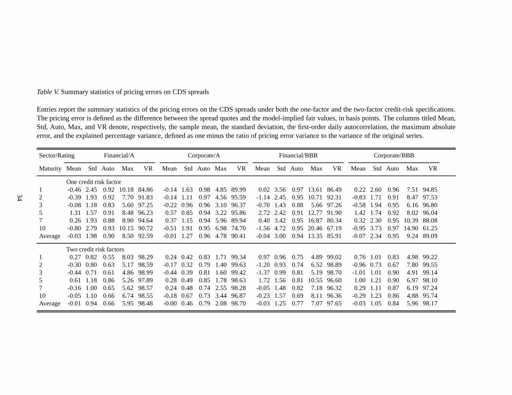
Table V.Summary statistics of pricing errors on CDS spreads

Entries report the summary statistics of the pricing errorson the CDS spreads under both the one-factor and the two-factor credit-risk specifications.The pricing error is defined as the difference between the spread quotes and the model-implied fair values, in basis points. The columns titled Mean,Std, Auto, Max, and VR denote, respectively, the sample mean, the standard deviation, the first-order daily autocorrelation, the maximum absoluteerror, and the explained percentage variance, defined as oneminus the ratio of pricing error variance to the variance of the original series.

Sector/Rating Financial/A Corporate/A Financial/BBB Corporate/BBB

Maturity Mean Std Auto Max VR Mean Std Auto Max VR Mean Std AutoMax VR Mean Std Auto Max VR

One credit risk factor1 -0.46 2.45 0.92 10.18 84.86 -0.14 1.63 0.98 4.85 89.99 0.02 3.56 0.97 13.61 86.49 0.22 2.60 0.96 7.51 94.852 -0.39 1.93 0.92 7.70 91.83 -0.14 1.11 0.97 4.56 95.59 -1.14 2.45 0.95 10.71 92.31 -0.83 1.71 0.91 8.47 97.533 -0.08 1.18 0.83 5.60 97.25 -0.22 0.96 0.96 3.10 96.37 -0.70 1.43 0.88 5.66 97.26 -0.58 1.94 0.95 6.16 96.805 1.31 1.57 0.91 8.48 96.23 0.57 0.85 0.94 3.22 95.86 2.72 2.420.91 12.77 91.90 1.42 1.74 0.92 8.02 96.047 0.26 1.93 0.88 8.90 94.64 0.37 1.15 0.94 5.96 89.94 0.40 3.420.95 16.87 80.34 0.32 2.30 0.95 10.39 88.0810 -0.80 2.79 0.93 10.15 90.72 -0.51 1.91 0.95 6.98 74.70 -1.56 4.72 0.95 20.46 67.19 -0.95 3.73 0.97 14.90 61.25Average -0.03 1.98 0.90 8.50 92.59 -0.01 1.27 0.96 4.78 90.41-0.04 3.00 0.94 13.35 85.91 -0.07 2.34 0.95 9.24 89.09

Two credit risk factors1 0.27 0.82 0.55 8.03 98.29 0.24 0.42 0.83 1.71 99.34 0.97 0.960.75 4.89 99.02 0.76 1.01 0.83 4.98 99.222 -0.30 0.80 0.63 5.17 98.59 -0.17 0.32 0.79 1.40 99.63 -1.20 0.93 0.74 6.52 98.89 -0.96 0.73 0.67 7.80 99.553 -0.44 0.71 0.61 4.86 98.99 -0.44 0.39 0.81 1.60 99.42 -1.37 0.99 0.81 5.19 98.70 -1.01 1.01 0.90 4.91 99.145 0.61 1.18 0.86 5.26 97.89 0.28 0.49 0.85 1.78 98.63 1.72 1.560.81 10.55 96.60 1.00 1.21 0.90 6.97 98.107 -0.16 1.00 0.65 5.62 98.57 0.24 0.48 0.74 2.55 98.28 -0.05 1.48 0.82 7.18 96.32 0.29 1.11 0.87 6.19 97.2410 -0.05 1.10 0.66 6.74 98.55 -0.18 0.67 0.73 3.44 96.87 -0.231.57 0.69 8.11 96.36 -0.29 1.23 0.86 4.88 95.74Average -0.01 0.94 0.66 5.95 98.48 -0.00 0.46 0.79 2.08 98.70-0.03 1.25 0.77 7.07 97.65 -0.03 1.05 0.84 5.96 98.17

34

Table VI.One-factor default arrival dynamics and the term structureof credit spreads

Entries report the parameter estimates and the standard errors (in parentheses) that determine the one-factordefault arrival dynamics and the term structure of credit spreads. Estimation is based on CDS spreads ateach of the four industry and credit rating classes with quasi-maximum likelihood method.

Parameters Financial-A Corporate-A Financial-BBB Corporate-BBB

β1 0.0341 ( 0.0097 ) -0.0607 ( 0.0070 ) -0.0198 ( 0.0138 ) -0.0572( 0.0086 )β2 -0.0117 ( 0.0088 ) 0.0109 ( 0.0062 ) 0.0009 ( 0.0150 ) -0.0159 (0.0106 )β3 0.0275 ( 0.0072 ) 0.0324 ( 0.0059 ) 0.0032 ( 0.0153 ) -0.0012 ( 0.0108 )κ1

yx -0.0063 ( 0.0178 ) 0.0279 ( 0.0133 ) -0.0016 ( 0.0260 ) -0.0442( 0.0156 )κ2

yx 0.0034 ( 0.0036 ) -0.0056 ( 0.0022 ) -0.0119 ( 0.0034 ) -0.0066( 0.0025 )κ3

yx 0.0091 ( 0.0007 ) 0.0062 ( 0.0004 ) 0.0218 ( 0.0028 ) -0.0040 ( 0.0020 )κy 0.0000 ( 0.0022 ) 0.0186 ( 0.0019 ) 0.1161 ( 0.0050 ) 0.1173 ( 0.0028 )σy 0.0012 ( 0.0000 ) 0.0007 ( 0.0000 ) 0.0017 ( 0.0001 ) 0.0015 ( 0.0001 )θy 0.0031 ( 0.0006 ) 0.0028 ( 0.0003 ) 0.0064 ( 0.0008 ) 0.0090 ( 0.0006 )γy -1.1642 ( 0.0839 ) -2.1864 ( 0.1611 ) -1.7724 ( 0.1356 ) -1.5849 ( 0.1100 )

Table VII.Two-factor default arrival dynamics and the term structureof credit spreads

Entries report the parameter estimates and and the standarderrors (in parentheses) that determine the two-factor default arrival dynamics and the term structure of credit spreads. Estimation is based on CDS spreadsat each of the four industry and credit rating classes with quasi-maximum likelihood method.

Parameters Financial-A Corporate-A Financial-BBB Corporate-BBB

β1 -0.0253 ( 0.0122 ) 0.0123 ( 0.0054 ) 0.0330 ( 0.0183 ) 0.0759 ( 0.0135 )β2 0.0772 ( 0.0098 ) -0.0392 ( 0.0053 ) 0.0325 ( 0.0184 ) -0.0293 (0.0138 )β3 -0.0346 ( 0.0091 ) 0.0007 ( 0.0052 ) -0.0110 ( 0.0154 ) -0.0004( 0.0095 )κ1

yx,1 -0.0594 ( 0.0172 ) 0.0532 ( 0.0087 ) -0.0448 ( 0.0317 ) 0.0031 (0.0237 )κ1

yx,2 0.0565 ( 0.0174 ) -0.0370 ( 0.0123 ) 0.0007 ( 0.0336 ) -0.0177 (0.0340 )κ2

yx,1 0.0166 ( 0.0048 ) 0.0205 ( 0.0030 ) 0.0088 ( 0.0062 ) 0.0220 ( 0.0051 )κ2

yx,2 0.0143 ( 0.0032 ) -0.0225 ( 0.0020 ) 0.0455 ( 0.0065 ) 0.0013 ( 0.0057 )κ3

yx,1 -0.0000 ( 0.0092 ) -0.0111 ( 0.0038 ) -0.0018 ( 0.0093 ) -0.0009 ( 0.0068 )κ3

yx,2 0.0068 ( 0.0017 ) -0.0012 ( 0.0014 ) 0.0232 ( 0.0041 ) 0.0113 ( 0.0041 )κy,1 0.2691 ( 0.0126 ) 0.2390 ( 0.0113 ) 0.1789 ( 0.0114 ) 0.1333 ( 0.0081 )κy,2 0.0000 ( 0.0045 ) 0.0630 ( 0.0061 ) 0.0237 ( 0.0089 ) 0.0077 ( 0.0074 )σy 0.0020 ( 0.0001 ) 0.0011 ( 0.0000 ) 0.0025 ( 0.0001 ) 0.0019 ( 0.0001 )θy 0.0048 ( 0.0005 ) 0.0032 ( 0.0003 ) 0.0070 ( 0.0008 ) 0.0084 ( 0.0005 )γy -0.5178 ( 0.0350 ) -1.0273 ( 0.0482 ) -0.3327 ( 0.0457 ) -0.3857 ( 0.0507 )

35

Table VIII.Summary statistics of pricing errors on libor, swap, and CDSspreads from joint estimation

Entries report the summary statistics of the pricing errorson the eurodollar libor, swap rates, and the averagecds spreads under a joint five-factor interest-rate and credit-spread model. We define the pricing error as thedifference between the observed time series and the model-implied fair values, in basis points. The columnstitled Mean, Std, Auto, Max, and VR denote, respectively, the sample mean, the standard deviation, the first-order daily autocorrelation, the maximum absolute error, and the explained percentage variance, defined asone minus the ratio of pricing error variance to the varianceof the original series, in percentages.

Libor/swap rates CDS spreads

Maturity Mean Std Auto Max VR Mean Std Auto Max VR

1 -0.01 0.65 0.04 2.46 100.00 0.24 0.56 0.76 2.79 99.452 0.20 1.34 0.60 6.03 99.99 -0.55 0.44 0.69 4.07 99.643 -0.28 0.73 0.68 3.47 100.00 -0.60 0.50 0.73 3.24 99.535 0.20 1.24 0.87 6.14 99.97 0.81 0.65 0.84 2.95 98.897 -0.06 0.65 0.83 2.68 99.99 -0.25 0.79 0.85 3.72 97.4610 -0.03 1.18 0.89 3.87 99.93 0.05 0.91 0.82 3.65 96.69Average 0.00 0.96 0.65 4.11 99.98 -0.05 0.64 0.78 3.40 98.61

Table IX.Joint dynamics of interest rate and credit risks

Entries report the parameter estimates and standard errors(in parentheses) that determine the joint dynamicsand term structure of the benchmark libor interest rates andthe aggregate CDS spreads. Estimation is basedon five interest rate series( 12-month libor and swap rates oftwo, three, five, seven, and ten years) and fiveCDS spread series at one,two, three, five, seven andten years.

Rates κr sκ θr σr γr

0.0067 16.8289 0.0571 0.0206 -0.4239( 0.0011 ) ( 1.4434 ) ( 0.0009 ) ( 0.0005 ) ( 0.0237 )

Credit κy,1 κy,2 θy σy γy

0.1813 0.1647 0.0031 0.0006 -0.7858( 0.0164 ) ( 0.0275 ) ( 0.0002 ) ( 0.0000 ) ( 0.0459 )

Interactions β κyx,1 κyx,2 κxy,1 κxy,2

0.0599 -0.0227 0.0410 -4.4772 -10.0956( 0.0059 ) ( 0.0046 ) ( 0.0016 ) ( 0.6935 ) ( 2.4083 )-0.0136 0.0341 -0.0142 2.5033 8.2421

( 0.0063 ) ( 0.0017 ) ( 0.0002 ) ( 0.1976 ) ( 0.5183 )0.0023 0.0147 0.0147 0.9713 -2.5709

( 0.0029 ) ( 0.0014 ) ( 0.0014 ) ( 0.1674 ) ( 0.5491 )

36

Table X.Sub-sampel parameter estimates on the joint dynamics of interest rate and credit risks

Entries report the sub-sample parameter estimates and standard errors (in parentheses) that determine the joint dynamics and term structure of thebenchmark libor interest rates and aggregate CDS spreads.

Sample May 2003 – July 2005 July 2005 – October 2007

Rates κr sκ θr σr γr κr sκ θr σr γr

0.0069 15.3572 0.0559 0.0182 -0.3739 0.0060 17.9024 0.11110.0226 -0.3618( 0.0029 ) ( 3.3414 ) ( 0.0022 ) ( 0.0010 ) ( 0.0436 ) ( 0.0007 ) ( 1.1247 ) ( 0.0051 ) ( 0.0006 ) ( 0.0398 )

Credit κy,1 κy,2 θy σy γy κy,1 κy,2 θy σy γy

0.1214 0.0003 0.0016 0.0008 -0.7041 0.0557 0.0000 0.0000 0.0004 -1.3197( 0.0228 ) ( 0.0553 ) ( 0.0004 ) ( 0.0001 ) ( 0.1610 ) ( 0.0143 ) ( 0.0137 ) ( 0.0004 ) ( 0.0000 ) ( 0.1564 )

Interactions β κyx,1 κyx,2 κxy,1 κxy,2 β κyx,1 κyx,2 κxy,1 κxy,2

-0.0230 0.0142 0.0275 -5.5422 -18.6046 0.0435 0.0216 0.0401 -4.1610 -5.0398( 0.0085 ) ( 0.0064 ) ( 0.0036 ) ( 0.9138 ) ( 3.4997 ) ( 0.0095 ) ( 0.0065 ) ( 0.0017 ) ( 0.4804 ) ( 1.4270 )

0.0142 0.0256 -0.0139 1.9579 6.0498 -0.0522 0.0269 -0.00572.2132 7.6024( 0.0106 ) ( 0.0016 ) ( 0.0007 ) ( 0.3803 ) ( 0.6548 ) ( 0.0082 ) ( 0.0009 ) ( 0.0001 ) ( 0.1180 ) ( 0.3520 )

0.0144 0.0064 0.0064 0.0484 -3.4561 -0.0027 0.0122 0.0122 1.0296 -7.9298( 0.0057 ) ( 0.0035 ) ( 0.0035 ) ( 0.2638 ) ( 0.8591 ) ( 0.0027 ) ( 0.0009 ) ( 0.0009 ) ( 0.2444 ) ( 0.8190 )

37

Table XI.Parameter estimates on the general Gaussian-affine specification

Entries report parameter estimates and standard errors (inparentheses) on a general three-factor Gaussian-affine specification on the term structure of interest rates.

κ κ+λ2 br λ1 ar

0.657 0 0(0.049) − −0.075 0.031 0(0.077) (0.002) −−0.335 −1.856 1.108(0.081 (0.078 (0.068)

0.102 0 0(0.004) − −−0.534 0.392 0(0.024) (0.006) −−1.001 −1.706 1.301(0.045 (0.054 (0.024)

0.0000(0.0000)0.0000(0.0000)0.0076(0.0002)

−0.279(0.005)−0.438(0.031)−1.467(0.061)

[

0.0012(0.0001)

]

Table XII. Summary statistics of pricing errors on the libor and swap rates from the general three-factorGaussian affine specification

Entries report the summary statistics of the pricing errorson the eurodollar libor and swap rates under thegeneral three-factor Gaussian affine specification. We define the pricing error as the difference betweenthe observed interest-rate quotes and the model-implied fair values in basis points. The columns titledMean, Std, Auto, Max, and VR denote, respectively, the sample mean, the standard deviation, the first-orderautocorrelation, the maximum absolute error, and the explained percentage variance, defined as one minusthe ratio of pricing error variance to interest-rate variance, in percentages.

Maturity Mean Std Auto Max VR

1 0.05 1.63 0.00 6.37 99.992 0.21 1.95 0.55 8.99 99.983 -0.30 1.14 0.50 6.02 99.995 0.19 1.33 0.87 7.62 99.977 -0.10 0.89 0.86 4.29 99.9810 0.04 1.34 0.85 4.49 99.91Average 0.01 1.38 0.61 6.30 99.97

38

Financial/A Financial/BBB

04 05 06 070

10

20

30

40

50

60

70

80

90

100

CD

S, B

ps

04 05 06 070

10

20

30

40

50

60

70

80

90

100

CD

S, B

ps

Corporate/A Corporate/BBB

04 05 06 070

10

20

30

40

50

60

70

80

90

100

CD

S, B

ps

04 05 06 070

10

20

30

40

50

60

70

80

90

100

CD

S, B

ps

Figure 1.Time series of average CDS spreads.Each panel represents one industry sector and one rating class. The six lines in each panel plot the time-series of the average quotes on CDS spreads at six fixed maturities. The solid lines represent the one-yearCDS series and the dash-dotted lines represent the 10-year CDS series. CDS series at intermediate maturitiesare in dashed lines.

39

04 05 06 070

1

2

3

4

5

6

Libo

r/swa

p, %

Figure 2.Time series of libor and swap rates.Lines plot the time series of the eurodollar libor and swap rates. The solid line denotes the 12-month liborseries, the dashed-dotted line denotes the 10-year swap rate series, and the remaining dashed line denoteswap rates with maturities from two to seven years.

40

1 2 3 4 5 6 7 8 9 10

0.1

0.2

0.3

0.4

0.5

0.6

0.7

0.8

0.9

Maturity, Years

Fact

or L

oadi

ng, %

Figure 3.Contemporaneous response of the forward rate curve to different frequency components.The three lines denote the contemporaneous response of the instantaneous forward rate curve to the threefrequency components in the benchmark interest-rate movements. The solid line denotes the response to thehighest frequency. The dashed line denotes the response to the intermediate frequency. The dash-dotted linedenotes the response to the lowest frequency.

41

Interest-rate factors Credit-risk factorsFinancial/A

1 2 3 4 5 6 7 8 9 10

−4

−2

0

2

4

6

8

10

12

Maturity, Years

Facto

r Loa

ding,

Bps

1 2 3 4 5 6 7 8 9 10

2

4

6

8

10

12

14

16

18

20

Maturity, Years

Facto

r Loa

ding,

Bps

Corporate/A

1 2 3 4 5 6 7 8 9 10−6

−5

−4

−3

−2

−1

0

1

2

3

Maturity, Years

Facto

r Loa

ding,

Bps

1 2 3 4 5 6 7 8 9 10

1

2

3

4

5

6

7

8

9

10

Maturity, Years

Facto

r Loa

ding,

Bps

Financial/BBB

1 2 3 4 5 6 7 8 9 10−12

−10

−8

−6

−4

−2

0

2

4

6

Maturity, Years

Facto

r Loa

ding,

Bps

1 2 3 4 5 6 7 8 9 10

5

10

15

20

25

Maturity, Years

Facto

r Loa

ding,

Bps

Corporate/BBB

1 2 3 4 5 6 7 8 9 10

−4

−2

0

2

4

6

8

10

12

Maturity, Years

Facto

r Loa

ding,

Bps

1 2 3 4 5 6 7 8 9 10

2

4

6

8

10

12

14

16

18

Maturity, Years

Facto

r Loa

ding,

Bps

Figure 4.Credit spread responses to one standard deviation moves in the interest-rate and credit-risk factors.Panels on the left side denote the contemporaneous responseof the forward default rate to one standarddeviation shocks from the three interest-rate factors. Panels on the right side denote the response of theforward default rate to one standard deviation moves from the two credit-risk factors. Within each panel,the frequencies of the factors decline from the solid line tothe dashed line and then to the dash-dotted line.

42

Interest-rate factors Credit-risk factors

1 2 3 4 5 6 7 8 9 10

20

40

60

80

100

120

140

160

180

200

Maturity, Years

Fact

or L

oadi

ng, B

ps

1 2 3 4 5 6 7 8 9 10

−50

−40

−30

−20

−10

0

Maturity, Years

Fact

or L

oadi

ng, B

ps

Figure 5.Contemporaneous responses of forward interest-rate curveto interest-rate and credit risk shocks.The three lines in the left panel plot the responses of the instantaneous forward rate curve to one standarddeviation movements in the three interest-rate factors. The two lines in the right panel plot the responses toone standard deviation movements in the two credit-risk factors. In each panel, the frequency declines fromthe solid line, to the dashed line, and then to the dash-dotted line.

43

Interest-rate factors Credit-risk factors

1 2 3 4 5 6 7 8 9 10−4

−2

0

2

4

6

8

10

12

Maturity, Years

Fact

or L

oadi

ng

1 2 3 4 5 6 7 8 9 10

−3

−2

−1

0

1

2

3

4

5

6

Maturity, Years

Fact

or L

oadi

ng

Figure 6.Contemporaneous responses of forward default rate to interest-rate and credit risk shocks.The three lines in the left panel plot the responses of the forward default rate to one standard deviationmovements in the three interest-rate factors. The two linesin the right panel plot the responses to onestandard deviation movements in the two credit-risk factors. In each panel, the frequency declines from thesolid line, to the dashed line, and then to the dash-dotted line.

44

Interest-rate factors Credit-risk factorsMay 2003 – July 2005

1 2 3 4 5 6 7 8 9 100

20

40

60

80

100

120

140

160

180

Maturity, Years

Fact

or L

oadi

ng, B

ps

1 2 3 4 5 6 7 8 9 10−40

−30

−20

−10

0

10

20

30

Maturity, Years

Fact

or L

oadi

ng, B

ps

July 2005 – October 2007

1 2 3 4 5 6 7 8 9 10

20

40

60

80

100

120

140

160

180

200

220

Maturity, Years

Fact

or L

oadi

ng, B

ps

1 2 3 4 5 6 7 8 9 10−35

−30

−25

−20

−15

−10

−5

0

Maturity, Years

Fact

or L

oadi

ng, B

ps

Figure 7. Contemporaneous responses of forward interest-rate curveto interest-rate and credit risk shocksat different sample periods.The left panels plot the responses of the instantaneous forward rate curve to one standard deviation move-ments in the three interest-rate factors. The right panels plot the responses to one standard deviation move-ments in the two credit-risk factors. In each panel, the frequency declines from the solid line, to the dashedline, and then to the dash-dotted line.

45

Interest-rate factors Credit-risk factorsMay 2003 – July 2005

1 2 3 4 5 6 7 8 9 10

−6

−4

−2

0

2

4

6

8

10

12

14

Maturity, Years

Fact

or L

oadi

ng

1 2 3 4 5 6 7 8 9 10−1

0

1

2

3

4

5

6

7

8

9

Maturity, Years

Fact

or L

oadi

ng

July 2005 – October 2007

1 2 3 4 5 6 7 8 9 10−15

−10

−5

0

5

10

15

Maturity, Years

Fact

or L

oadi

ng

1 2 3 4 5 6 7 8 9 10−4

−2

0

2

4

6

8

10

12

14

Maturity, Years

Fact

or L

oadi

ng

Figure 8. Contemporaneous responses of forward default rate to interest-rate and credit risk shocks atdifferent sample periods.The left panels plot the responses of the forward default rate to one standard deviation movements in thethree interest-rate factors. The right panels plot the responses to one standard deviation movements in thetwo credit-risk factors. In each panel, the frequency declines from the solid line, to the dashed line, and thento the dash-dotted line.

46

dynamic interactions between interest-rate and credit...

Documents