dynamic scheduling of multiproduct pipelines with...
TRANSCRIPT
A
sdmkueuwmts©
K
1
ltwlsblotbgttt
0d
Available online at www.sciencedirect.com
Computers and Chemical Engineering 32 (2008) 728–753
Dynamic scheduling of multiproduct pipelineswith multiple delivery due dates
Diego C. Cafaro, Jaime Cerda ∗INTEC (UNL - CONICET), Guemes 3450, 3000 Santa Fe, Argentina
Received 13 June 2006; received in revised form 27 February 2007; accepted 1 March 2007Available online 12 March 2007
bstract
Scheduling product batches in pipelines is a very complex task with many constraints to be considered. Several papers have been published on theubject during the last decade. Most of them are based on large-size MILP discrete time scheduling models whose computational efficiency greatlyiminishes for rather long time horizons. Recently, an MILP continuous problem representation in both time and volume providing better schedules atuch lower computational cost has been published. However, all model-based scheduling techniques were applied to examples assuming a static mar-
et environment, a short single-period time horizon and a unique due-date for all deliveries at the horizon end. In contrast, pipeline operators generallyse a monthly planning horizon divided into a number of equal-length periods and a cyclic scheduling strategy to fulfill terminal demands at periodnds. Moreover, the rerouting of shipments and time-dependent product requirements at distribution terminals force the scheduler to continuouslypdate pipeline operations. To address such big challenges facing the pipeline industry, this work presents an efficient MILP continuous-time frame-
ork for the dynamic scheduling of pipelines over a multiperiod moving horizon. At the completion time of the current period, the planning horizonoves forward and the re-scheduling process based on updated problem data is triggered again over the new horizon. Pumping runs may extend overwo or more periods and a different sequence of batches may be injected at each one. The approach has successfully solved a real-world pipelinecheduling problem involving the transportation of four products to five destinations over a rolling horizon always comprising four 1-week periods.
2007 Elsevier Ltd. All rights reserved.
ILP a
cbosodsactb2a
eywords: Multiproduct pipeline; Dynamic scheduling; Multiple due dates; M
. Introduction
Pipelines are the safest and least expensive way to deliverarge quantities of energy products from refineries to distributionerminals but at the same time the slowest form of transportationith speeds of 3–8 mph. Pipeline low costs mostly result from
ittle product damage along the trip, substantial economies ofcale, no need for containers moving with the cargo and noackhauls (Trench, 2001). In addition, the cargo movement isess affected by traffic and weather conditions compared withther modes of transportation. Nearly 68% of the intercityon-miles of crude oil and refined products in the US are handledy pipelines. The transportation of refined petroleum productsenerally combines a long-distance delivery by pipeline from
he refinery to distribution terminals followed by a truck journeyo local markets. Moreover, a single delivery from a refineryo a distant distribution terminal may require multiple pipeline∗ Corresponding author. Tel.: +54 342 4559175; fax: +54 342 4550944.E-mail address: [email protected] (J. Cerda).
pspsspo
098-1354/$ – see front matter © 2007 Elsevier Ltd. All rights reserved.oi:10.1016/j.compchemeng.2007.03.002
pproach
arriers. Liquid products are propelled through pipelinesy centrifugal pumps which are sited at pumping stations,ne at the origin and the others distributed along the pipelineeparated by a distance varying from 20 to 100 miles, dependingn the topography and the capacity requirement. Petroleumerivatives are inserted in the line one after another without anyeparation device between batches. If two consecutive productsre dissimilar, such as gasoline and jet fuel, a hybrid productalled transmix is created by intermixing at the interface. Theransmix must be separated and stored in a small holding tankefore sending back to the refinery for reprocessing (Hull,005). Pipelines are generally owned by a number of companiesnd most of them are common carriers transporting petroleumroducts from different refiners. A pipeline network can haveeveral entry and exit points and the interchange of refinedroducts between two common carrier pipelines may occur at
hared terminals. In this paper, the multiperiod scheduling of aingle unidirectional pipeline system involving a unique entryoint at the origin and several exit points as many as the numberf distribution terminals along the line is studied.
D.C. Cafaro, J. Cerda / Computers and Chemical Engineering 32 (2008) 728–753 729
Nomenclature
SetsI chronologically arranged batches (Iold ∪ Inew)Inew new batches to be injected during the time horizonIold old batches inside the pipeline at the start of the
time horizonJ distribution terminals along the pipelineJp distribution terminals demanding product pP refined petroleum productsR scheduled production runs at the oil refineryT time periods of the planning horizonTHF hard frozen periods on the planning horizonTSF soft frozen periods on the planning horizon
Parametersar, br starting/finishing time of the refinery production
run rcbp,j,t unit backorder penalty cost to tardily meet a
requirement due at period tcfp,p′ unit reprocessing cost of interface material involv-
ing products p and p′cidp,j unit inventory holding cost for product p at depot
jcirp unit inventory holding cost for product p in refin-
ery tankscpp,j unit normal pumping cost to deliver product p
from the refinery to depot jddt upper extreme of period tdemp,j,t overall demand of product p to be satisfied at
depot j before due date ddt
Dmax maximum delivery size from a batch to a distri-bution terminal
Foi current upper pipeline coordinate of old batch i
hf number of hard-frozen time periodshmax horizon lengthht time period lengthhwmax maximum working time(IDmax)p,j maximum allowed inventory level for product
p at depot j(IDmin)p,j minimum allowed inventory level for product p
at depot jIFp,p′ volume of interface between batches containing
products p and p′IRo
p initial inventory of product p in refinery tanks(IRmax)p maximum allowed refinery inventory level for
product p(IRmin)p minimum allowed refinery inventory level for
product pk current time periodlmin, lmax minimum/maximum length of a new batch injec-
tionN number of time periods in the rolling horizonNS/CSp,j,t sizes of new/cancelled nominations for product
p due at period t in terminal jPHmax accumulated daily peak hours
Qmax maximum injection sizesr size of the refinery production run rsf number of soft-frozen time periodsvb pumping ratesvmp,j maximum supply rate of product p to the local
market from depot jvpr production rate for run rWo
i current volume of old batch iρ unit-time penalty cost for operating during peak-
hour intervalsσj volumetric coordinate of depot j from the head
terminalτp,p′ changeover time between injections of products
p and p′
Continuous variablesBp,j,t backorder of product p for depot j due at period t
to meet at period t + 1Ci, Li completion time/length of pumping run i ∈ Inew
D(i′)i,j volume of batch i diverted to depot j while inject-
ing batch i′
DM(i′)p,j amount of product p sent to local market j during
the time interval [Ci′−1, Ci′ ]
DP(i′)i,p,j amount of product p supplied by batch i to depot
j ∈ Jp during [Ci′ − Li′ , Ci′ ]
F(i′)i upper coordinate of batch i from the origin at time
Ci′
ID(i′)p,j inventory of product p in depot j at the end of
pumping run i′IRF(i′)
p inventory of product p in refinery at the end ofpumping run i′
IRS(i′)p inventory of product p in refinery at the start of
pumping run i′PH peak-hour usageQi initial size of the new batch iQPi,p volume of product p injected in the pipeline while
pumping batch iSLi,r production output from run r ∈ R available in
refinery tanks at time Ci
SUi,r production output from run r ∈ R available inrefinery tanks at time (Ci − Li)
W(i′)i size of batch i at time Ci′
WIFi,p,p′ interface volume between batches i and (i − 1)containing products p and p′
Binary variableswi,t denoting that the injection of batch i ends within
time period t
x(i′)i,j denoting that a portion of batch i can be trans-
ferred to depot j while injecting i′yi,p denoting that batch i contains product pzli,r denoting that injection i ends after the refinery
production run r has started
730 D.C. Cafaro, J. Cerda / Computers and Chem
1p
uiFtatbhGnsiicooespuodaciiopra
ratAtfd
tcamtanopbvMifnptd
1
p(lastoabapsn2Icntajts
zui,r denoting that injection i begins after the refineryproduction run r has ended
.1. Batch scheduling and dispatching in multiproductipeline systems
The scheduling of pipelines transporting petroleum prod-cts from a single refinery to multiple destinations has receivedncreasing attention among researchers in the last decade (seeig. 1). Usually, customers contact the pipeline carrier to place
heir transport orders or “nominations” for the next month. Oncecustomer nominates to a particular pipeline and the nomina-
ion has been accepted, the customer must make the batch toe shipped available in the pipeline origin at the right time andave sufficient storage capacity to receive it at the destination.enerally, batch movements in a particular month must be nomi-ated by the 25th of the previous month. Afterwards, the pipelinecheduler develops a detailed hourly schedule of pipeline activ-ties over a monthly horizon. To do that, the scheduling horizons first divided into a number of cycles or periods with a typicalycle length of 7, 10 or 14 days, i.e. a multiperiod horizon. More-ver, a customer nomination is partitioned into as many portionsf equal size as the number of cycles or periods per month, andach portion is due at the end of a cycle. In other words, a cycliccheduling approach is usually applied by assuming the sameroduct demand profile at every period. Once a complete prod-ct sequence has been shipped during a cycle, a second identicalne is started (Sheppard, 1984). If a pipeline operates on a 14-ay cycle, the shipper must provide storage capacity to receivebatch that will cover his demands for 14 days. With a 7-day
ycle, the customer only needs half as much tankage, but thenterface volume will duplicate. Therefore, the storage capac-ty to be provided by the customer is reduced at the expensef increased interface reprocessing costs. If nominations exceedumping capacity, schedulers must decide which nominations toeduce through the so-called “apportionment” process by usingpportionment rules (Hull, 2005).
The pipeline schedule is executed by dispatchers whoemotely perform loading, transportation and unloading oper-tions in a fully automated way through computers all fromhe control room. By using the Supervisory Control and Data
cquisition system (SCADA) estimating batch arrival times toerminals and batch sizes from the information given by inter-ace detectors, dispatchers can trace batches along the line andivert them to one or more terminal tankages. In this manner,
Fig. 1. A single unidirectional multiproduct pipeline system.
ldncatFdapst
ical Engineering 32 (2008) 728–753
hey continually monitor each batch to ensure that the physicalonnection to tankage or other pipelines is open when the batchrrives to the stated terminal (Rabinow, 2004). The entire lineust be stopped when a customer cannot receive his shipment at
he stated destination because of insufficient tankage capacity orny other practical inconvenience. Similarly to real-life termi-al operations, a good problem representation should be capablef tracing batches while flowing inside the pipeline in order torecisely establish (i) the earliest time at which the delivery of aatch to the stated terminal can be started and (ii) the time inter-al during which the batch has access to the terminal tankage.oreover, terminals usually have a few tanks just used to facil-
tate loading/unloading operations rather than being employedor long-term storage. Therefore, a key issue for efficient termi-al operations is the coordination among incoming and outgoingroduct flows to/from every tank. Product stock-outs at the headerminal or overloading conditions at other depots oblige theispatcher to temporarily stop the line.
.2. Previous contributions and new challenges
Two different types of scheduling methodologies have beenroposed in the literature: knowledge-based search techniquesSasikumar, Prakash, Patil, & Ramani, 1997) and mixed-integerinear mathematical programming (MILP) formulations. Allpproaches assume a single-period planning horizon and thepecification of a unique due-date for all product demands athe different depots, i.e. just at the horizon end. Dependingn whether or not the pipeline volume and the time horizonre both discretized, model-based scheduling methods cane grouped into two classes: discrete and continuous MILPpproaches. Most of the proposed optimization models not onlyartitioned the horizon into time intervals of equal or unequalizes but also the pipeline volume is divided into a significantumber of single-product packs (Magatao, Arruda, & Neves,004; Neiro & Pinto, 2004; Rejowski & Pinto, 2003, 2004).n contrast, Cafaro and Cerda (2004) developed a novel MILPontinuous formulation that requires neither time discretizationor pipeline division. In comparison with heuristic searchechniques, one of the major drawbacks of the optimizationpproaches is the use of rather short time horizons comprisingust a few days to limit the size of the mathematical model. Inhis way, the solution time remains reasonable and the optimalolution can be efficiently found.
One of the challenges on pipeline operation is to meetarge product demands from every depot along the pipeline atifferent due-dates over rather long planning horizons. Sinceew transportation requests are placed by customers as time pro-eeds, the information on the problem is indeed time-dependentnd the pipeline schedule should be periodically updated. Addi-ional “nominations” may arrive at any time within the month.urthermore, some old nominations can be cancelled or theirestinations could be changed by the shippers while the batches
re already in transit. The pipeline scheduler is not only alanner but also a revisor of plans since it is necessary to updatechedules to meet shipper requirements in a profitable way forhe carrier. Rerouting of shipments is said to be a fact of life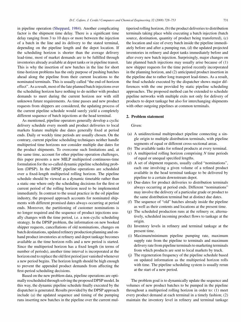
Chem
ifdodtliTtanetdurtd
dmecmtttflosaciimenassbhaSnhatfi
mtdir
ttstaialnittfappw
2
D.C. Cafaro, J. Cerda / Computers and
n pipeline operation (Sheppard, 1984). Another complicatingactor is the shipment time delay. There is a significant timeelay ranging from 3 to 10 days or more between the injectionf a batch in the line and its delivery to the stated terminal,epending on the pipeline length and the depot location. Ifhe scheduling horizon is shorter than the average deliveryead-time, most of market demands are to be fulfilled throughnventories already available at depot tanks or in pipeline transit.his is why the insertion of new batches in the line for short
ime-horizon problems has the only purpose of pushing batcheshead along the pipeline from their current locations to theominated terminals. This is usually called “the end-of-horizonffect”. As a result, most of the late planned batch injections overhe scheduling horizon have nothing to do neither with productemands to meet during the current horizon nor with stillnknown future requirements. As time passes and new productequests from shippers are considered, the updating process ofhe current pipeline schedule would surely yield a completelyifferent sequence of batch injections at the head terminal.
As mentioned, pipeline operators generally develop a cyclicelivery schedule every month and product deliveries to localarkets feature multiple due dates generally fixed at period
nds. Daily or weekly time periods are usually chosen. On theontrary, current pipeline scheduling techniques neither handleultiperiod time horizons nor consider multiple due dates for
he product shipments. To overcome such limitations and, athe same time, account for other pipeline operation challenges,his paper presents a new MILP multiperiod continuous-timeormulation for the so-called dynamic pipeline scheduling prob-em (DPSP). In the DPSP, pipeline operations are scheduledver a fixed-length multiperiod rolling horizon. The pipelinechedule should be viewed as a dynamic timetable rather thanstatic one where only the scheduling decisions for the first or
urrent period of the rolling horizon need to be implementedmmediately. In contrast to the usual practice in the oil pipelinendustry, the proposed approach accounts for nominated ship-
ents with different promised dates always occurring at periodnds. Moreover, the partitioning of customer nominations iso longer required and the sequence of product injections usu-lly changes with the time period, i.e. a non-cyclic schedulingtrategy. In the DPSP problem, the information on new bookedhipper requests, cancellations of old nominations, changes onatch destinations, updated refinery production planning and on-and product inventories at refinery and depot tankage becomesvailable as the time horizon rolls and a new period is started.ince the multiperiod horizon has a fixed length (in terms ofumber of periods), another time interval is incorporated at theorizon end to replace the old first period just vanished whenevernew period begins. The horizon length should be high enough
o prevent the appended product demands from affecting therst-period scheduling decisions.
Based on the new problem data, pipeline operations are opti-ally rescheduled through solving the proposed DPSP model. In
his way, the dynamic pipeline schedule finally executed by theispatcher is generated. Results provided by the DPSP approachnclude (a) the updated sequence and timing of the pumpinguns inserting new batches in the pipeline over the current mul-
vtem
ical Engineering 32 (2008) 728–753 731
iperiod rolling horizon, (b) the product deliveries to distributionerminals taking place while executing a batch injection (batchource, destination, quantity of product being transferred), (c)he location and size of every batch inside the pipeline immedi-tely before and after a pumping run, (d) the updated projectednventories in refinery and depot tanks immediately before andfter every new batch injection. Surprisingly, major changes onate planned batch injections may usually arise because of (1)ew shipper requests for the time period recently incorporatedn the planning horizon, and (2) anticipated product insertion inhe pipeline due to rather long transport lead-times. As a result,he final schedule executed by the dispatcher shows major dif-erences with the one provided by static pipeline schedulingpproaches. The proposed method can be extended to scheduleipeline networks with multiple exits not only for delivery ofroducts to depot tankage but also for interchanging shipmentsith other outgoing pipelines at common terminals.
. Problem statement
Given:
(a) A unidirectional multiproduct pipeline connecting a sin-gle origin to multiple distribution terminals, with pipelinesegments of equal or different cross-sectional areas.
(b) The available tanks for refined products at every terminal.(c) A multiperiod rolling horizon comprising N time periods
of equal or unequal specified lengths.(d) A set of shipment requests, usually called “nominations”,
each one involving a given volume of a refined productavailable in the head terminal tankage to be delivered bypipeline to a certain downstream depot.
(e) Due-dates for product deliveries to distribution terminalsalways occurring at period ends. Different “nominations”may involve the delivery of a particular grade or product tothe same distribution terminal but at distinct due dates.
(f) The sequence of “old” batches already inside the pipelineas well as their contents and locations at the present time.
(g) The scheduled production runs at the refinery or, alterna-tively, scheduled incoming product flows to tankage at theorigin.
(h) Inventory levels in refinery and terminal tankage at thepresent time.
(i) Maximum/minimum pipeline pumping rate, maximumsupply rate from the pipeline to terminals and maximumdelivery rate from pipeline terminals to marketing terminalsfrom which products are sent to local markets by truck.
(j) The regeneration frequency of the pipeline schedule basedon updated information as the multiperiod horizon rollswith time. The pipeline scheduling system is usually rerunat the start of a new period.
The problem goal is to dynamically update the sequence and
olumes of new product batches to be pumped in the pipelinehroughout a multiperiod rolling horizon in order to: (1) meetvery product demand at each terminal in a timely fashion; (2)aintain the inventory level in refinery and terminal tankage
7 Chem
wetTps
3
(
(
(
(
(
4
uo((ttitpfantpeirlt
32 D.C. Cafaro, J. Cerda / Computers and
ithin the permissible ranges; (3) trace the size and location ofvery batch in pipeline transit; (4) minimize the sum of pumping,ransition, down-time, backorder and inventory carrying costs.he pipeline schedule should indicate the amount and type ofroduct to be pumped, the batch pumping rate as well as thetarting and completion time of every batch injection.
. Model assumptions
(1) A single multiproduct transmission pipeline with unidirec-tional flow, conveying refined petroleum products from arefinery to several downstream terminals is considered.
(2) The pipeline remains completely full of products at anytime. By assuming liquid incompressibility, the only wayto get a volume of product out of the line at a downstreamterminal is by injecting an equal volume at the origin.
(3) The pipeline operates in fungible mode. If individualbatches of the same grade or product from different ship-pers meet common specifications, they can be mixed intoa consolidated or fungible batch and sent through thepipeline as a single batch.
(4) Each fungible batch can be allocated to two or more ter-minals. As new product batches are injected, a portion ofa batch flowing through the pipeline can be diverted tothe assigned terminal while the remainder will continuemoving to more distant points, i.e. the so-called batch“stripping” operation.
(5) The individual batches flowing together on a fungible batchcan be dynamically allocated to distribution terminals; i.e.allocation of batches to terminals can be modified duringthe rescheduling process. Dynamic allocation is requiredbecause a batch while in transit along the line can be tradedto another shipper at a different destination.
(6) A product request at some distribution terminal can besatisfied by diverting material from more than one fungiblebatch.
(7) Product batches are sequentially pumped into the pipelineat turbulent flow to retard mixing.
(8) The transmix or contamination volume between a partic-ular pair of refined products is supposed to be a knownconstant, independent of the scheduled batch movements.The transmix is kept into the line until it reaches the farthestterminal where it is stored and rerouted to the refinery. Oth-erwise, the interface would be automatically regenerated,thus increasing transition costs.
(9) A portion of a batch can be delivered to a terminal onlyif (a) the batch has arrived to the point on the line wherethe physical connection to the terminal tankage is avail-able and (b) a tank in the terminal is ready to store thebatch. If a terminal cannot receive a shipment of prod-uct because of insufficient capacity in the assigned tank,then the entire line must be stopped until the problem is
solved.10) The unit pumping cost is a known constant that varies withthe product and the stated destination but it is independentof the pump rate.
htti
ical Engineering 32 (2008) 728–753
11) The maximum supply rate of refined products to refinerytanks from scheduled production runs is always lesser thanthe lowest pipeline pumping rate. If several refiners makeuse of the pipeline, the product batches to be shipped areassumed to be available at the head terminal tankage at thestart time of the batch injections. In the examples involvinga single refinery, the maximum production rate is about500 m3/h, whereas the minimum pump rate into a 20 in.pipeline is over 800 m3/h.
12) A non-cycling pipeline schedule strategy over a multi-period rolling horizon is applied. Therefore, the sequenceof product shipments to be executed by the dispatcher mayvary from one to the next period.
13) The present time is the beginning of the most immediateperiod of the current rolling horizon, i.e. the first period.The planned product shipments for the first period of thetime horizon (the action period) are not subject to changesduring the periodic scheduling review. New transportationrequests can be accepted just for late periods. First-periodshipments are the only ones executed by the dispatcher. Theimplementation of planned shipments for a later periodmust wait until it becomes the first period of the rollinghorizon.
14) Since it may take over 1 or 2 weeks to move a batchfrom the origin to the assigned terminal (the delivery lead-time), the horizon length must exceed the largest deliverylead-time. Otherwise, batches will be put in the pipelineduring the action period without knowing their exactdestinations.
. Major model variables and constraints
The mathematical formulation for the dynamic multiprod-ct pipeline scheduling problem (DPSP) is defined in termsf four major sets: (a) the old and new fungible batchesi ∈ I = Iold ∪ Inew), (b) the pipeline distribution terminals (j ∈ J),c) the refined petroleum products to be delivered (p ∈ P) fromhe refinery to terminals along the line and (d) the time periodsaking part of the multiperiod rolling horizon (t ∈ T). Old batches∈ Iold are those already in transit along the line at the presentime, while new fungibles batches i ∈ Inew are planned to beumped in the pipeline at future periods. Moreover, the problemormulation will assume that the set I has been chronologicallyrranged beforehand with the old batches i ∈ Iold preceding theew batches i ∈ Inew. Therefore, the first entry in Iold is the far-hest old batch from the origin while the last entry is the batchut in the pipeline more recently. On the other hand, the firstlement of Inew corresponds to the first batch to be injected dur-ng the current horizon while the last one is the latest pumpingun being planned. Then, the insertion of a new batch i in theine should start after ending the injection of batch (i − 1). Sincehe number of pumping runs to be executed throughout the time
orizon is unknown beforehand but lower than |Inew|, some ofhe later entries of Inew are never executed, i.e. they stand for fic-itious new batches. Some criteria for choosing |Inew| are givenn Section 6.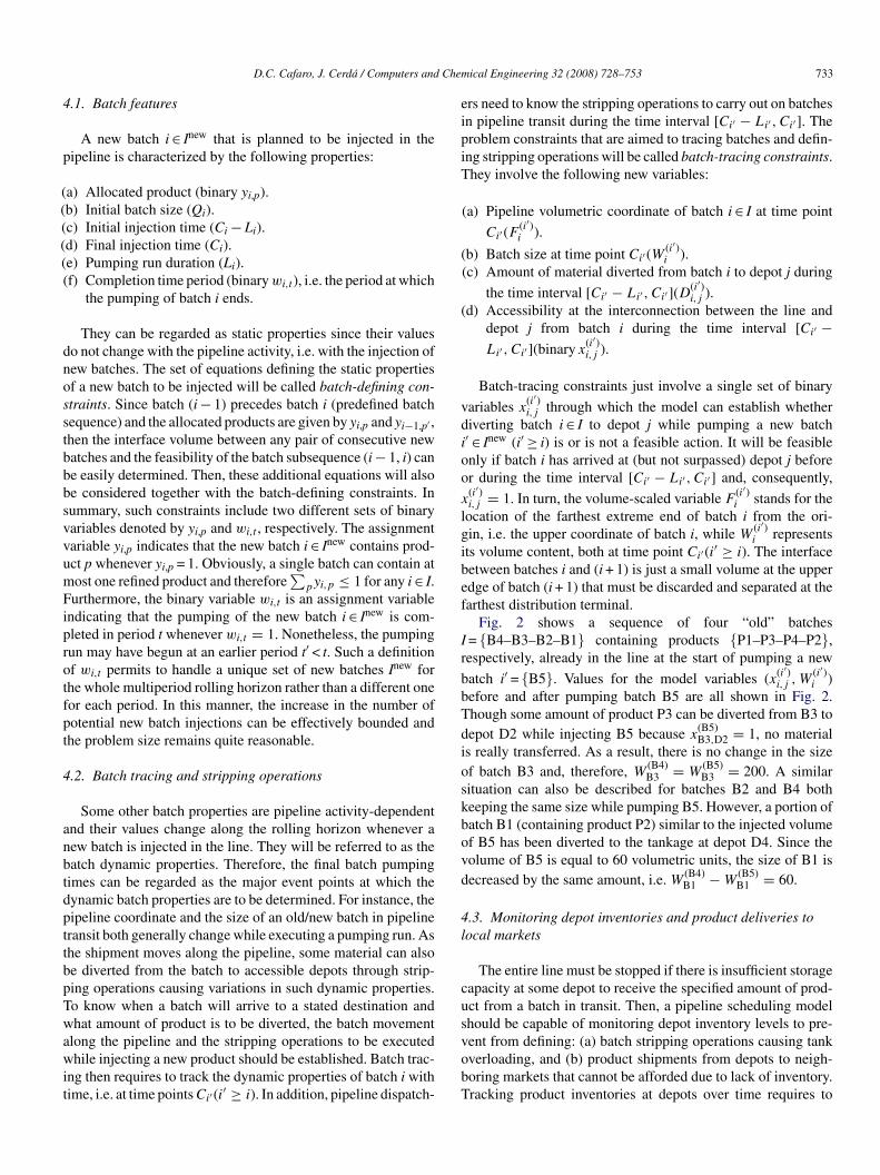
Chem
4
p
((((((
dnosstbbbsvvumFiprotfpt
4
anbtdpttbpTwawit
eipiT
(
(
vdioo
x
lgibef
Ir
bbTdioskbovd
4l
cus
D.C. Cafaro, J. Cerda / Computers and
.1. Batch features
A new batch i ∈ Inew that is planned to be injected in theipeline is characterized by the following properties:
a) Allocated product (binary yi,p).b) Initial batch size (Qi).c) Initial injection time (Ci − Li).d) Final injection time (Ci).e) Pumping run duration (Li).f) Completion time period (binary wi,t), i.e. the period at which
the pumping of batch i ends.
They can be regarded as static properties since their valueso not change with the pipeline activity, i.e. with the injection ofew batches. The set of equations defining the static propertiesf a new batch to be injected will be called batch-defining con-traints. Since batch (i − 1) precedes batch i (predefined batchequence) and the allocated products are given by yi,p and yi−1,p′ ,hen the interface volume between any pair of consecutive newatches and the feasibility of the batch subsequence (i − 1, i) cane easily determined. Then, these additional equations will alsoe considered together with the batch-defining constraints. Inummary, such constraints include two different sets of binaryariables denoted by yi,p and wi,t , respectively. The assignmentariable yi,p indicates that the new batch i ∈ Inew contains prod-ct p whenever yi,p = 1. Obviously, a single batch can contain atost one refined product and therefore
∑pyi,p ≤ 1 for any i ∈ I.
urthermore, the binary variable wi,t is an assignment variablendicating that the pumping of the new batch i ∈ Inew is com-leted in period t whenever wi,t = 1. Nonetheless, the pumpingun may have begun at an earlier period t′ < t. Such a definitionf wi,t permits to handle a unique set of new batches Inew forhe whole multiperiod rolling horizon rather than a different oneor each period. In this manner, the increase in the number ofotential new batch injections can be effectively bounded andhe problem size remains quite reasonable.
.2. Batch tracing and stripping operations
Some other batch properties are pipeline activity-dependentnd their values change along the rolling horizon whenever aew batch is injected in the line. They will be referred to as theatch dynamic properties. Therefore, the final batch pumpingimes can be regarded as the major event points at which theynamic batch properties are to be determined. For instance, theipeline coordinate and the size of an old/new batch in pipelineransit both generally change while executing a pumping run. Ashe shipment moves along the pipeline, some material can alsoe diverted from the batch to accessible depots through strip-ing operations causing variations in such dynamic properties.o know when a batch will arrive to a stated destination andhat amount of product is to be diverted, the batch movement
long the pipeline and the stripping operations to be executedhile injecting a new product should be established. Batch trac-
ng then requires to track the dynamic properties of batch i withime, i.e. at time points Ci′ (i′ ≥ i). In addition, pipeline dispatch-
vobT
ical Engineering 32 (2008) 728–753 733
rs need to know the stripping operations to carry out on batchesn pipeline transit during the time interval [Ci′ − Li′ , Ci′ ]. Theroblem constraints that are aimed to tracing batches and defin-ng stripping operations will be called batch-tracing constraints.hey involve the following new variables:
(a) Pipeline volumetric coordinate of batch i ∈ I at time point
Ci′ (F(i′)i ).
b) Batch size at time point Ci′ (W(i′)i ).
(c) Amount of material diverted from batch i to depot j during
the time interval [Ci′ − Li′ , Ci′ ](D(i′)i,j ).
d) Accessibility at the interconnection between the line anddepot j from batch i during the time interval [Ci′ −Li′ , Ci′ ](binary x
(i′)i,j ).
Batch-tracing constraints just involve a single set of binary
ariables x(i′)i,j through which the model can establish whether
iverting batch i ∈ I to depot j while pumping a new batch′ ∈ Inew (i′ ≥ i) is or is not a feasible action. It will be feasiblenly if batch i has arrived at (but not surpassed) depot j beforer during the time interval [Ci′ − Li′ , Ci′ ] and, consequently,(i′)i,j = 1. In turn, the volume-scaled variable F
(i′)i stands for the
ocation of the farthest extreme end of batch i from the ori-in, i.e. the upper coordinate of batch i, while W
(i′)i represents
ts volume content, both at time point Ci′ (i′ ≥ i). The interfaceetween batches i and (i + 1) is just a small volume at the upperdge of batch (i + 1) that must be discarded and separated at thearthest distribution terminal.
Fig. 2 shows a sequence of four “old” batches= {B4–B3–B2–B1} containing products {P1–P3–P4–P2},espectively, already in the line at the start of pumping a new
atch i′ = {B5}. Values for the model variables (x(i′)i,j , W
(i′)i )
efore and after pumping batch B5 are all shown in Fig. 2.hough some amount of product P3 can be diverted from B3 toepot D2 while injecting B5 because x
(B5)B3,D2 = 1, no material
s really transferred. As a result, there is no change in the sizef batch B3 and, therefore, W
(B4)B3 = W
(B5)B3 = 200. A similar
ituation can also be described for batches B2 and B4 botheeping the same size while pumping B5. However, a portion ofatch B1 (containing product P2) similar to the injected volumef B5 has been diverted to the tankage at depot D4. Since theolume of B5 is equal to 60 volumetric units, the size of B1 isecreased by the same amount, i.e. W
(B4)B1 − W
(B5)B1 = 60.
.3. Monitoring depot inventories and product deliveries toocal markets
The entire line must be stopped if there is insufficient storageapacity at some depot to receive the specified amount of prod-ct from a batch in transit. Then, a pipeline scheduling modelhould be capable of monitoring depot inventory levels to pre-
ent from defining: (a) batch stripping operations causing tankverloading, and (b) product shipments from depots to neigh-oring markets that cannot be afforded due to lack of inventory.racking product inventories at depots over time requires to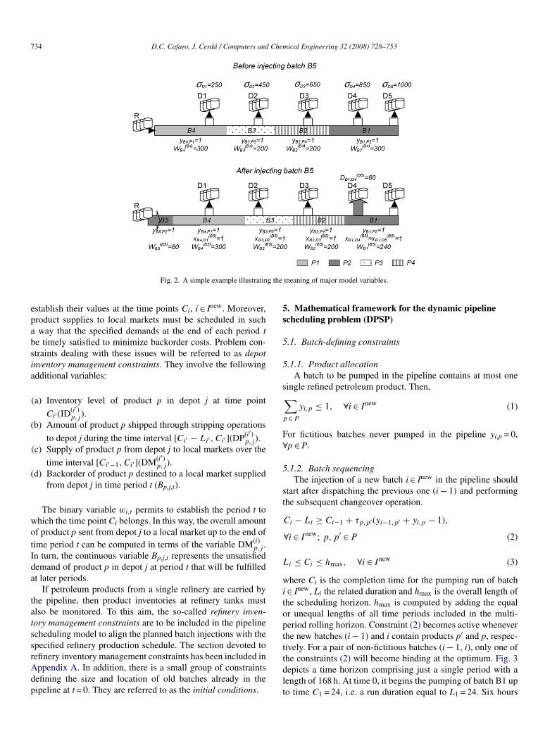
734 D.C. Cafaro, J. Cerda / Computers and Chemical Engineering 32 (2008) 728–753
g the
epabsia
(
(
wotIda
tatssrAdp
5s
5
5
s
p
F∀
5
st
L
witoptt
Fig. 2. A simple example illustratin
stablish their values at the time points Ci, i ∈ Inew. Moreover,roduct supplies to local markets must be scheduled in suchway that the specified demands at the end of each period t
e timely satisfied to minimize backorder costs. Problem con-traints dealing with these issues will be referred to as depotnventory management constraints. They involve the followingdditional variables:
(a) Inventory level of product p in depot j at time point
Ci′ (ID(i′)p,j).
b) Amount of product p shipped through stripping operations
to depot j during the time interval [Ci′ − Li′ , Ci′ ](DP(i′)p,j).
(c) Supply of product p from depot j to local markets over the
time interval [Ci′−1, Ci′ ](DM(i′)p,j).
d) Backorder of product p destined to a local market suppliedfrom depot j in time period t (Bp,j,t).
The binary variable wi,t permits to establish the period t tohich the time point Ci belongs. In this way, the overall amountf product p sent from depot j to a local market up to the end ofime period t can be computed in terms of the variable DM(i)
p,j .n turn, the continuous variable Bp,j,t represents the unsatisfiedemand of product p in depot j at period t that will be fulfilledt later periods.
If petroleum products from a single refinery are carried byhe pipeline, then product inventories at refinery tanks mustlso be monitored. To this aim, the so-called refinery inven-ory management constraints are to be included in the pipelinecheduling model to align the planned batch injections with thepecified refinery production schedule. The section devoted to
efinery inventory management constraints has been included inppendix A. In addition, there is a small group of constraintsefining the size and location of old batches already in theipeline at t = 0. They are referred to as the initial conditions.tdlt
meaning of major model variables.
. Mathematical framework for the dynamic pipelinecheduling problem (DPSP)
.1. Batch-defining constraints
.1.1. Product allocationA batch to be pumped in the pipeline contains at most one
ingle refined petroleum product. Then,∑∈ P
yi,p ≤ 1, ∀i ∈ Inew (1)
or fictitious batches never pumped in the pipeline yi,p = 0,p ∈ P.
.1.2. Batch sequencingThe injection of a new batch i ∈ Inew in the pipeline should
tart after dispatching the previous one (i − 1) and performinghe subsequent changeover operation.
Ci − Li ≥ Ci−1 + τp,p′ (yi−1,p′ + yi,p − 1),
∀i ∈ Inew; p, p′ ∈ P (2)
i ≤ Ci ≤ hmax, ∀i ∈ Inew (3)
here Ci is the completion time for the pumping run of batch∈ Inew, Li the related duration and hmax is the overall length ofhe scheduling horizon. hmax is computed by adding the equalr unequal lengths of all time periods included in the multi-eriod rolling horizon. Constraint (2) becomes active wheneverhe new batches (i − 1) and i contain products p′ and p, respec-ively. For a pair of non-fictitious batches (i − 1, i), only one of
he constraints (2) will become binding at the optimum. Fig. 3epicts a time horizon comprising just a single period with aength of 168 h. At time 0, it begins the pumping of batch B1 upo time C1 = 24, i.e. a run duration equal to L1 = 24. Six hours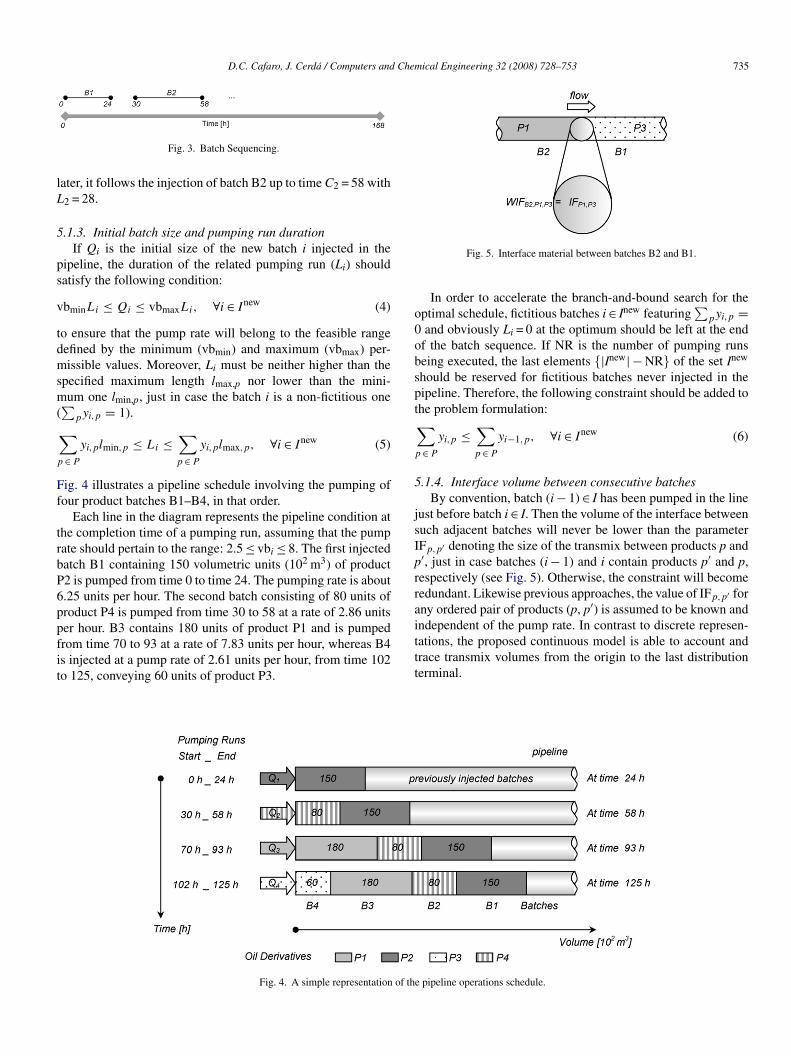
D.C. Cafaro, J. Cerda / Computers and Chemical Engineering 32 (2008) 728–753 735
lL
5
ps
v
tdmsm(
p
Ff
trbP6ppfit
o0obspt
p
5
jsIprra
Fig. 3. Batch Sequencing.
ater, it follows the injection of batch B2 up to time C2 = 58 with2 = 28.
.1.3. Initial batch size and pumping run durationIf Qi is the initial size of the new batch i injected in the
ipeline, the duration of the related pumping run (Li) shouldatisfy the following condition:
bminLi ≤ Qi ≤ vbmaxLi, ∀i ∈ Inew (4)
o ensure that the pump rate will belong to the feasible rangeefined by the minimum (vbmin) and maximum (vbmax) per-issible values. Moreover, Li must be neither higher than the
pecified maximum length lmax,p nor lower than the mini-um one lmin,p, just in case the batch i is a non-fictitious one∑
pyi,p = 1).∑∈ P
yi,plmin,p ≤ Li ≤∑p ∈ P
yi,plmax,p, ∀i ∈ Inew (5)
ig. 4 illustrates a pipeline schedule involving the pumping ofour product batches B1–B4, in that order.
Each line in the diagram represents the pipeline condition athe completion time of a pumping run, assuming that the pumpate should pertain to the range: 2.5 ≤ vbi ≤ 8. The first injectedatch B1 containing 150 volumetric units (102 m3) of product2 is pumped from time 0 to time 24. The pumping rate is about.25 units per hour. The second batch consisting of 80 units ofroduct P4 is pumped from time 30 to 58 at a rate of 2.86 units
er hour. B3 contains 180 units of product P1 and is pumpedrom time 70 to 93 at a rate of 7.83 units per hour, whereas B4s injected at a pump rate of 2.61 units per hour, from time 102o 125, conveying 60 units of product P3.ittt
Fig. 4. A simple representation of the
Fig. 5. Interface material between batches B2 and B1.
In order to accelerate the branch-and-bound search for theptimal schedule, fictitious batches i ∈ Inew featuring
∑pyi,p =
and obviously Li = 0 at the optimum should be left at the endf the batch sequence. If NR is the number of pumping runseing executed, the last elements {|Inew| − NR} of the set Inew
hould be reserved for fictitious batches never injected in theipeline. Therefore, the following constraint should be added tohe problem formulation:∑∈ P
yi,p ≤∑p ∈ P
yi−1,p, ∀i ∈ Inew (6)
.1.4. Interface volume between consecutive batchesBy convention, batch (i − 1) ∈ I has been pumped in the line
ust before batch i ∈ I. Then the volume of the interface betweenuch adjacent batches will never be lower than the parameterFp,p′ denoting the size of the transmix between products p and′, just in case batches (i − 1) and i contain products p′ and p,espectively (see Fig. 5). Otherwise, the constraint will becomeedundant. Likewise previous approaches, the value of IFp,p′ forny ordered pair of products (p, p′) is assumed to be known and
ndependent of the pump rate. In contrast to discrete represen-ations, the proposed continuous model is able to account andrace transmix volumes from the origin to the last distributionerminal.pipeline operations schedule.
7 Chem
W
∀BwbtsriTd2aas
5
uspf
y
5
amttprvahipnuc
i
5b
mzupodbp
vb
cC
t
spad
tctitdpt
t
cc
C
C
ONfit
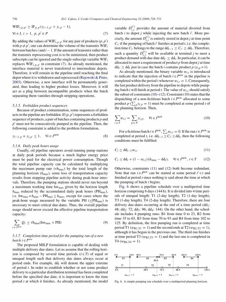
hoTd4ut1palthough it has begun in the previous one. The third run finishesat time period T3 (wB3,T3 = 1) and the last one is completed inT4 (wB4,T4 = 1).
36 D.C. Cafaro, J. Cerda / Computers and
IFi,p,p′ ≥ IFp,p′ (yi−1,p′ + yi,p − 1),
i ∈ I, i > 1, p, p′ ∈ P (7)
y adding the values of WIFi,p,p′ for any pair of products (p, p′)ith p = p′, one can determine the volume of the transmix WIFi
etween batches i and i − 1. If the amount of transmix rather thanhe transmix reprocessing cost is to be minimized, then productubscripts can be ignored and the single-subscript variable WIFi
eplaces WIFi,p,p′ in constraint (7). As already mentioned, thenterface material is never transferred to intermediate depots.herefore, it will remain in the pipeline until reaching the finalepot where it is withdrawn and reprocessed (Rejowski & Pinto,003). Otherwise, a new interface will be permanently gener-ted, thus leading to higher product losses. Moreover, it willct as a plug between incompatible products when the batcheparating them vanishes through stripping operations.
.1.5. Forbidden product sequencesBecause of product contamination, some sequences of prod-
cts in the pipeline are forbidden. If (p, p′) represents a forbiddenequence of products, a pair of batches containing products p and′ must not be consecutively pumped in the pipeline. Then, theollowing constraint is added to the problem formulation,
i−1,p + yi,p′ ≤ 1, ∀i ∈ Inew (8)
.1.6. Daily peak hours usageUsually, oil pipeline operators avoid running pump stations
t daily peak periods because a much higher energy priceust be paid for the electrical power consumption. Though
he total pipeline capacity can be calculated by multiplyinghe maximum pump rate (vbmax) by the total length of thelanning horizon (hmax), some loss of transportation capacityesults from stopping pipeline activity during peak-hour inter-als. Therefore, the pumping stations should never run beyondmaximum working time hwmax given by the horizon length
max reduced by the accumulated daily peak hours (PHmax),.e. hwmax = hmax − PHmax ≤ hmax, except for cases where theeak-hour usage measured by the variable PH (≤PHmax) isecessary to meet critical due-dates. Thus, the overall pipelinesage should never exceed the effective pipeline transportationapacity:∑∈ Inew
Qi ≤ vbmax(hwmax + PH) (9)
.1.7. Completion time period for the pumping run of a newatch i ∈ Inew
The proposed MILP formulation is capable of dealing withultiple delivery due-dates. Let us assume that the rolling hori-
on is composed by several time periods (t ∈ T) of equal ornequal length such that delivery due dates always occur ateriod ends. For example, ddt will denote the upper extreme
f period t. In order to establish whether or not some productelivery to a particular distribution terminal has been completedefore the specified due date, it is important to know the timeeriod t at which it finishes. As already mentioned, the model Fical Engineering 32 (2008) 728–753
ariable D(i′)i,j provides the amount of material diverted from
atch i to depot j while injecting the new batch i′. More pre-
isely, the amount D(i′)i,j is entirely stored in depot j at time point
i′ if the pumping of batch i′ finishes at period t, i.e. the comple-ion time Ci′ belongs to the range ddt−1 ≤ Ci′ ≤ ddt . Therefore,
uch a quantity D(i′)i,j will be available at terminal j to meet a
roduct demand with due date ddt′ ≥ ddt . In particular, it can bellocated to meet a requirement of product p from depot j at timedt′ ≥ ddt just in case the batch i contains product p (yi,p = 1).
As already mentioned, the binary variable wi,t is introducedo indicate that the injection of batch i ∈ Inew in the pipeline isompleted within the period t whenever wi,t = 1. Consequently,he last product delivery from the pipeline to depots while pump-ng batch i will finish at period t. The value of wi,t should satisfyhe subset of constraints (10)–(12). Constraint (10) states that theispatching of a non-fictitious batch i ∈ Inew allocated to someroduct p (
∑pyi,p = 1) must be completed at some period t of
he planning horizon. Then,
∑∈ T
wi,t =∑p ∈ P
yi,p, ∀i ∈ Inew (10)
For a fictitious batch i ∈ Inew,∑
twi,t = 0. If the run i ∈ Inew isompleted at period t, i.e. ddt−1 ≤ Ci′ ≤ ddt, then the followingonditions must be fulfilled:
i ≥ ddt−1wi,t (11)
i ≤ ddt + (1 − wi,t) (hmax − ddt), ∀i ∈ Inew, t ∈ T (12)
therwise, constraints (11) and (12) both become redundant.ote that run i ∈ Inew can be started at some period t′ < t andnished at period t since nothing is said about the time at which
he pumping of batch i begins.Fig. 6 shows a pipeline schedule over a multiperiod time
orizon comprising 6 days (144 h). It is divided into 4 time peri-ds of unequal length: T1 (2-day length), T2 (1-day length),3 (1-day length), T4 (2-day length). Therefore, there are fourelivery due-dates occurring at the end of a time period (dd1:8; dd2: 72; dd3: 96; dd4: 144). On the other hand, the sched-le includes 4 pumping runs: B1 from time 0 to 23, B2 fromime 35 to 65, B3 from time 70 to 93 and B4 from time 102 to25. By definition, the first pumping run is completed at timeeriod T1 (wB1,T1 = 1) and the second ends at T2 (wB2,T2 = 1),
ig. 6. A simple pumping run schedule over a multiperiod planning horizon.
Chemical Engineering 32 (2008) 728–753 737
5
5C
iC
b
(
s
pbb(
F
F
dlim
F
CutF
5w
csfdt
Q
Ctpd
A
u
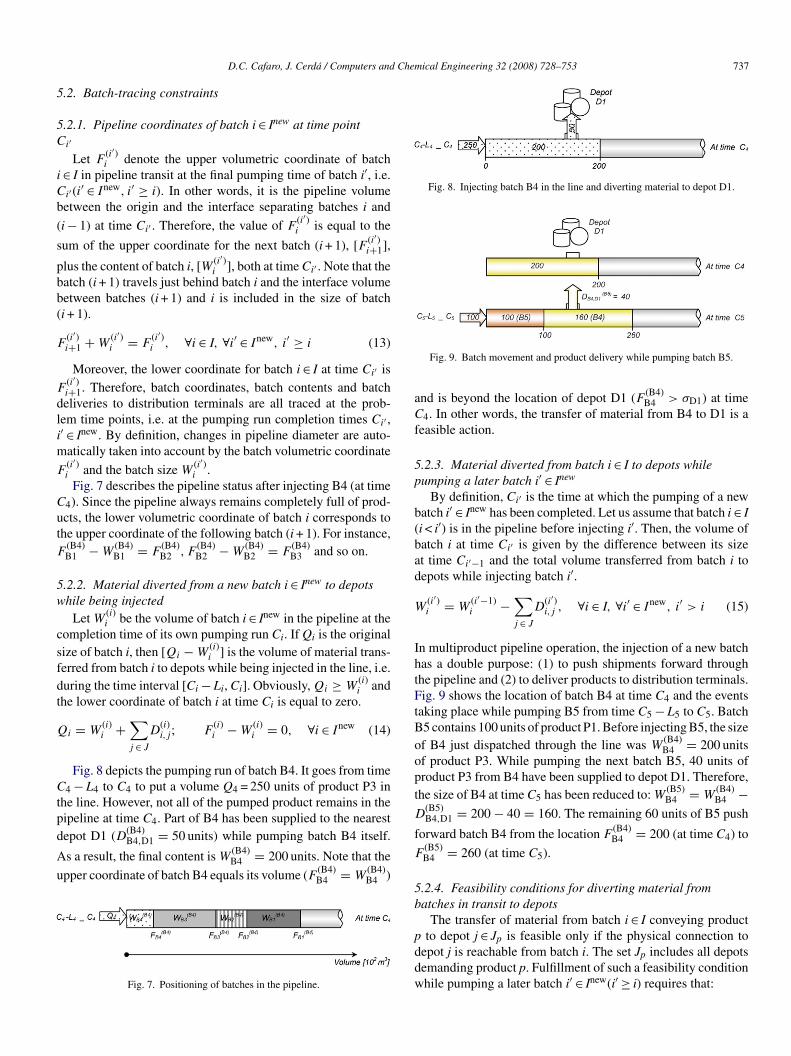
Fig. 8. Injecting batch B4 in the line and diverting material to depot D1.
aCf
5p
b(bad
W
IhtFtBoopt
D
D.C. Cafaro, J. Cerda / Computers and
.2. Batch-tracing constraints
.2.1. Pipeline coordinates of batch i ∈ Inew at time pointi′
Let F(i′)i denote the upper volumetric coordinate of batch
∈ I in pipeline transit at the final pumping time of batch i′, i.e.i′ (i′ ∈ Inew, i′ ≥ i). In other words, it is the pipeline volumeetween the origin and the interface separating batches i and
i − 1) at time Ci′ . Therefore, the value of F(i′)i is equal to the
um of the upper coordinate for the next batch (i + 1), [F (i′)i+1],
lus the content of batch i, [W (i′)i ], both at time Ci′ . Note that the
atch (i + 1) travels just behind batch i and the interface volumeetween batches (i + 1) and i is included in the size of batchi + 1).
(i′)i+1 + W
(i′)i = F
(i′)i , ∀i ∈ I, ∀i′ ∈ Inew, i′ ≥ i (13)
Moreover, the lower coordinate for batch i ∈ I at time Ci′ is(i′)i+1. Therefore, batch coordinates, batch contents and batcheliveries to distribution terminals are all traced at the prob-em time points, i.e. at the pumping run completion times Ci′ ,′ ∈ Inew. By definition, changes in pipeline diameter are auto-
atically taken into account by the batch volumetric coordinate(i′)i and the batch size W
(i′)i .
Fig. 7 describes the pipeline status after injecting B4 (at time4). Since the pipeline always remains completely full of prod-cts, the lower volumetric coordinate of batch i corresponds tohe upper coordinate of the following batch (i + 1). For instance,
(B4)B1 − W
(B4)B1 = F
(B4)B2 , F
(B4)B2 − W
(B4)B2 = F
(B4)B3 and so on.
.2.2. Material diverted from a new batch i ∈ Inew to depotshile being injected
Let W(i)i be the volume of batch i ∈ Inew in the pipeline at the
ompletion time of its own pumping run Ci. If Qi is the originalize of batch i, then [Qi − W
(i)i ] is the volume of material trans-
erred from batch i to depots while being injected in the line, i.e.uring the time interval [Ci − Li, Ci]. Obviously, Qi ≥ W
(i)i and
he lower coordinate of batch i at time Ci is equal to zero.
i = W(i)i +
∑j ∈ J
D(i)i,j; F
(i)i − W
(i)i = 0, ∀i ∈ Inew (14)
Fig. 8 depicts the pumping run of batch B4. It goes from time4 − L4 to C4 to put a volume Q4 = 250 units of product P3 in
he line. However, not all of the pumped product remains in theipeline at time C4. Part of B4 has been supplied to the nearest
epot D1 (D(B4)B4,D1 = 50 units) while pumping batch B4 itself.
s a result, the final content is W(B4)B4 = 200 units. Note that the
pper coordinate of batch B4 equals its volume (F (B4)B4 = W
(B4)B4 )
Fig. 7. Positioning of batches in the pipeline.
f
F
5b
pddw
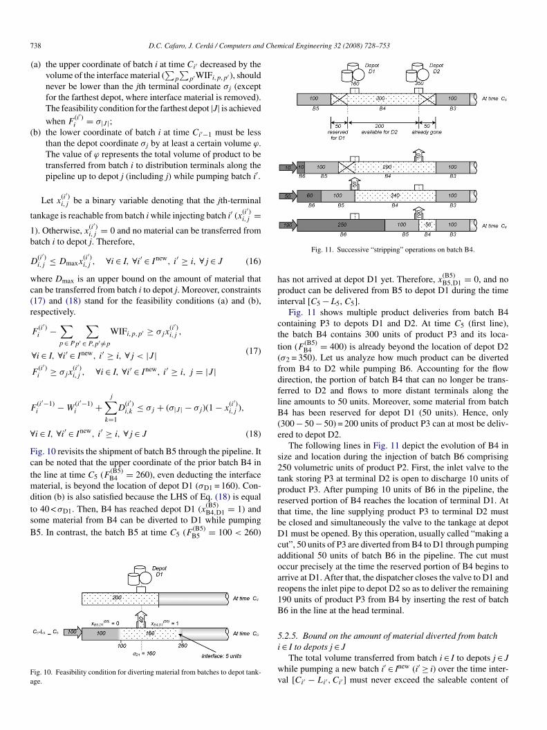
Fig. 9. Batch movement and product delivery while pumping batch B5.
nd is beyond the location of depot D1 (F (B4)B4 > σD1) at time
4. In other words, the transfer of material from B4 to D1 is aeasible action.
.2.3. Material diverted from batch i ∈ I to depots whileumping a later batch i′ ∈ Inew
By definition, Ci′ is the time at which the pumping of a newatch i′ ∈ Inew has been completed. Let us assume that batch i ∈ Ii < i′) is in the pipeline before injecting i′. Then, the volume ofatch i at time Ci′ is given by the difference between its sizet time Ci′−1 and the total volume transferred from batch i toepots while injecting batch i′.
(i′)i = W
(i′−1)i −
∑j ∈ J
D(i′)i,j , ∀i ∈ I, ∀i′ ∈ Inew, i′ > i (15)
n multiproduct pipeline operation, the injection of a new batchas a double purpose: (1) to push shipments forward throughhe pipeline and (2) to deliver products to distribution terminals.ig. 9 shows the location of batch B4 at time C4 and the events
aking place while pumping B5 from time C5 − L5 to C5. Batch5 contains 100 units of product P1. Before injecting B5, the sizef B4 just dispatched through the line was W
(B4)B4 = 200 units
f product P3. While pumping the next batch B5, 40 units ofroduct P3 from B4 have been supplied to depot D1. Therefore,he size of B4 at time C5 has been reduced to: W
(B5)B4 = W
(B4)B4 −
(B5)B4,D1 = 200 − 40 = 160. The remaining 60 units of B5 push
orward batch B4 from the location F(B4)B4 = 200 (at time C4) to
(B5)B4 = 260 (at time C5).
.2.4. Feasibility conditions for diverting material fromatches in transit to depots
The transfer of material from batch i ∈ I conveying productto depot j ∈ Jp is feasible only if the physical connection to
epot j is reachable from batch i. The set Jp includes all depotsemanding product p. Fulfillment of such a feasibility conditionhile pumping a later batch i′ ∈ Inew(i′ ≥ i) requires that:
7 Chemical Engineering 32 (2008) 728–753
(
t
1b
D
wc(r
F
∀FctmdtsB
Fa
hpi
ctt(fdflB(e
s2tp
38 D.C. Cafaro, J. Cerda / Computers and
(a) the upper coordinate of batch i at time Ci′ decreased by thevolume of the interface material (
∑p
∑p′WIFi,p,p′ ), should
never be lower than the jth terminal coordinate σj (exceptfor the farthest depot, where interface material is removed).The feasibility condition for the farthest depot |J| is achieved
when F(i′)i = σ|J |;
b) the lower coordinate of batch i at time Ci′−1 must be lessthan the depot coordinate σj by at least a certain volume ϕ.The value of ϕ represents the total volume of product to betransferred from batch i to distribution terminals along thepipeline up to depot j (including j) while pumping batch i′.
Let x(i′)i,j be a binary variable denoting that the jth-terminal
ankage is reachable from batch i while injecting batch i′ (x(i′)i,j =
). Otherwise, x(i′)i,j = 0 and no material can be transferred from
atch i to depot j. Therefore,
(i′)i,j ≤ Dmaxx
(i′)i,j , ∀i ∈ I, ∀i′ ∈ Inew, i′ ≥ i, ∀j ∈ J (16)
here Dmax is an upper bound on the amount of material thatan be transferred from batch i to depot j. Moreover, constraints17) and (18) stand for the feasibility conditions (a) and (b),espectively.
F(i′)i −
∑p ∈ P
∑p′ ∈ P,p′ =p
WIFi,p,p′ ≥ σjx(i′)i,j ,
∀i ∈ I, ∀i′ ∈ Inew, i′ ≥ i, ∀j < |J |F
(i′)i ≥ σjx
(i′)i,j , ∀i ∈ I, ∀i′ ∈ Inew, i′ ≥ i, j = |J |
(17)
(i′−1)i − W
(i′−1)i +
j∑k=1
D(i′)i,k ≤ σj + (σ|J | − σj)(1 − x
(i′)i,j ),
i ∈ I, ∀i′ ∈ Inew, i′ ≥ i, ∀j ∈ J (18)
ig. 10 revisits the shipment of batch B5 through the pipeline. Itan be noted that the upper coordinate of the prior batch B4 inhe line at time C5 (F (B5)
B4 = 260), even deducting the interfaceaterial, is beyond the location of depot D1 (σD1 = 160). Con-
ition (b) is also satisfied because the LHS of Eq. (18) is equalo 40 < σD1. Then, B4 has reached depot D1 (x(B5)
B4,D1 = 1) andome material from B4 can be diverted to D1 while pumping5. In contrast, the batch B5 at time C5 (F (B5)
B5 = 100 < 260)
ig. 10. Feasibility condition for diverting material from batches to depot tank-ge.
rtbDcaoar1B
5i
wv
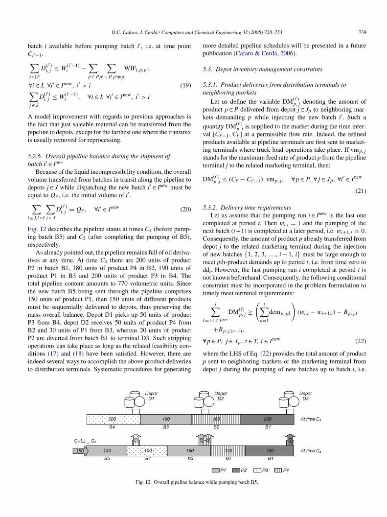
Fig. 11. Successive “stripping” operations on batch B4.
as not arrived at depot D1 yet. Therefore, x(B5)B5,D1 = 0, and no
roduct can be delivered from B5 to depot D1 during the timenterval [C5 − L5, C5].
Fig. 11 shows multiple product deliveries from batch B4ontaining P3 to depots D1 and D2. At time C5 (first line),he batch B4 contains 300 units of product P3 and its loca-ion (F (B5)
B4 = 400) is already beyond the location of depot D2σ2 = 350). Let us analyze how much product can be divertedrom B4 to D2 while pumping B6. Accounting for the flowirection, the portion of batch B4 that can no longer be trans-erred to D2 and flows to more distant terminals along theine amounts to 50 units. Moreover, some material from batch4 has been reserved for depot D1 (50 units). Hence, only
300 − 50 − 50) = 200 units of product P3 can at most be deliv-red to depot D2.
The following lines in Fig. 11 depict the evolution of B4 inize and location during the injection of batch B6 comprising50 volumetric units of product P2. First, the inlet valve to theank storing P3 at terminal D2 is open to discharge 10 units ofroduct P3. After pumping 10 units of B6 in the pipeline, theeserved portion of B4 reaches the location of terminal D1. Athat time, the line supplying product P3 to terminal D2 muste closed and simultaneously the valve to the tankage at depot1 must be opened. By this operation, usually called “making a
ut”, 50 units of P3 are diverted from B4 to D1 through pumpingdditional 50 units of batch B6 in the pipeline. The cut mustccur precisely at the time the reserved portion of B4 begins torrive at D1. After that, the dispatcher closes the valve to D1 andeopens the inlet pipe to depot D2 so as to deliver the remaining90 units of product P3 from B4 by inserting the rest of batch6 in the line at the head terminal.
.2.5. Bound on the amount of material diverted from batch
∈ I to depots j ∈ JThe total volume transferred from batch i ∈ I to depots j ∈ Jhile pumping a new batch i′ ∈ Inew (i′ ≥ i) over the time inter-al [Ci′ − Li′ , Ci′ ] must never exceed the saleable content of
Chem
bC
Atpi
5b
vde
i
Fir
tPptt1mmPBPodit
mp
5
5n
pk
qvpist
D
5
cnCdomdnct
�
D.C. Cafaro, J. Cerda / Computers and
atch i available before pumping batch i′, i.e. at time pointi′−1.∑
j<|J |D
(i′)i,j ≤ W
(i′−1)i −
∑p ∈ P
∑p′ ∈ P,p′ =p
WIFi,p,p′ ,
∀i ∈ I, ∀i′ ∈ Inew, i′ > i∑j ∈ J
D(i′)i,j ≤ W
(i′−1)i , ∀i ∈ I, ∀i′ ∈ Inew, i′ > i
(19)
model improvement with regards to previous approaches ishe fact that just saleable material can be transferred from theipeline to depots, except for the farthest one where the transmixs usually removed for reprocessing.
.2.6. Overall pipeline balance during the shipment ofatch i′ ∈ Inew
Because of the liquid incompressibility condition, the overallolume transferred from batches in transit along the pipeline toepots j ∈ J while dispatching the new batch i′ ∈ Inew must bequal to Qi′ , i.e. the initial volume of i′.∑∈ I,i≤i′
∑j ∈ J
D(i′)i,j = Qi′ , ∀i′ ∈ Inew (20)
ig. 12 describes the pipeline status at times C4 (before pump-ng batch B5) and C5 (after completing the pumping of B5),espectively.
As already pointed out, the pipeline remains full of oil deriva-ives at any time. At time C4 there are 200 units of product2 in batch B1, 180 units of product P4 in B2, 190 units ofroduct P1 in B3 and 200 units of product P3 in B4. Theotal pipeline content amounts to 770 volumetric units. Sincehe new batch B5 being sent through the pipeline comprises50 units of product P1, then 150 units of different productsust be sequentially delivered to depots, thus preserving theass overall balance. Depot D1 picks up 50 units of product3 from B4, depot D2 receives 50 units of product P4 from2 and 30 units of P1 from B3, whereas 20 units of product2 are diverted from batch B1 to terminal D3. Such stripping
perations can take place as long as the related feasibility con-itions (17) and (18) have been satisfied. However, there arendeed several ways to accomplish the above product deliverieso distribution terminals. Systematic procedures for generating∀wpd
Fig. 12. Overall pipeline balance
ical Engineering 32 (2008) 728–753 739
ore detailed pipeline schedules will be presented in a futureublication (Cafaro & Cerda, 2006).
.3. Depot inventory management constraints
.3.1. Product deliveries from distribution terminals toeighboring markets
Let us define the variable DM(i′)p,j denoting the amount of
roduct p ∈ P delivered from depot j ∈ Jp to neighboring mar-ets demanding p while injecting the new batch i′. Such a
uantity DM(i′)p,j is supplied to the market during the time inter-
al [Ci′−1, Ci′ ] at a permissible flow rate. Indeed, the refinedroducts available at pipeline terminals are first sent to market-ng terminals where truck load operations take place. If vmp,j
tands for the maximum feed rate of product p from the pipelineerminal j to the related marketing terminal, then:
M(i′)p,j ≤ (Ci′ − Ci′−1) vmp,j, ∀p ∈ P, ∀j ∈ Jp, ∀i′ ∈ Inew
(21)
.3.2. Delivery time requirementsLet us assume that the pumping run i ∈ Inew is the last one
ompleted at period t. Then wi,t = 1 and the pumping of theext batch (i + 1) is completed at a later period, i.e. wi+1,t = 0.onsequently, the amount of product p already transferred fromepot j to the related marketing terminal during the injectionf new batches {1, 2, 3, . . ., i − 1, i} must be large enough toeet pth-product demands up to period t, i.e. from time zero to
dt. However, the last pumping run i completed at period t isot known beforehand. Consequently, the following conditionalonstraint must be incorporated in the problem formulation toimely meet terminal requirements:
i∑=1 � ∈ Inew
DM(�)p,j ≥
(t∑
k=1
demp,j,k
)(wi,t − wi+1,t) − Bp,j,t
+Bp,j,(t−1),
new
p ∈ P, j ∈ Jp, t ∈ T, i ∈ I (22)here the LHS of Eq. (22) provides the total amount of productsent to neighboring markets or the marketing terminal from
epot j during the pumping of new batches up to batch i, i.e.
while pumping batch B5.
7 Chem
wtdotitrdpf
aIpzpoFappt
i
Ffi((pCbwowBT
twpasotitt
5
ainsaeiimdlp
40 D.C. Cafaro, J. Cerda / Computers and
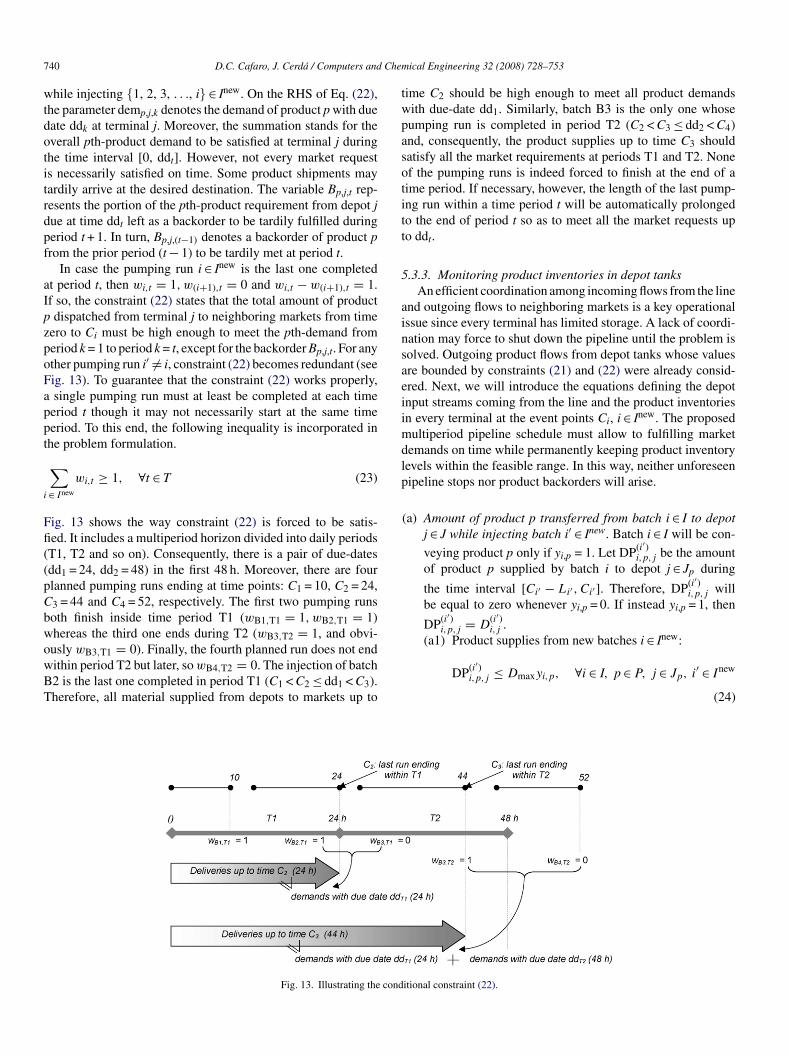
hile injecting {1, 2, 3, . . ., i}∈ Inew. On the RHS of Eq. (22),he parameter demp,j,k denotes the demand of product p with dueate ddk at terminal j. Moreover, the summation stands for theverall pth-product demand to be satisfied at terminal j duringhe time interval [0, ddt]. However, not every market requests necessarily satisfied on time. Some product shipments mayardily arrive at the desired destination. The variable Bp,j,t rep-esents the portion of the pth-product requirement from depot jue at time ddt left as a backorder to be tardily fulfilled duringeriod t + 1. In turn, Bp,j,(t−1) denotes a backorder of product prom the prior period (t − 1) to be tardily met at period t.
In case the pumping run i ∈ Inew is the last one completedt period t, then wi,t = 1, w(i+1),t = 0 and wi,t − w(i+1),t = 1.f so, the constraint (22) states that the total amount of productdispatched from terminal j to neighboring markets from time
ero to Ci must be high enough to meet the pth-demand fromeriod k = 1 to period k = t, except for the backorder Bp,j,t. For anyther pumping run i′ = i, constraint (22) becomes redundant (seeig. 13). To guarantee that the constraint (22) works properly,single pumping run must at least be completed at each time
eriod t though it may not necessarily start at the same timeeriod. To this end, the following inequality is incorporated inhe problem formulation.
∑∈ Inew
wi,t ≥ 1, ∀t ∈ T (23)
ig. 13 shows the way constraint (22) is forced to be satis-ed. It includes a multiperiod horizon divided into daily periodsT1, T2 and so on). Consequently, there is a pair of due-datesdd1 = 24, dd2 = 48) in the first 48 h. Moreover, there are fourlanned pumping runs ending at time points: C1 = 10, C2 = 24,3 = 44 and C4 = 52, respectively. The first two pumping runsoth finish inside time period T1 (wB1,T1 = 1, wB2,T1 = 1)hereas the third one ends during T2 (wB3,T2 = 1, and obvi-
usly wB3,T1 = 0). Finally, the fourth planned run does not endithin period T2 but later, so wB4,T2 = 0. The injection of batch2 is the last one completed in period T1 (C1 < C2 ≤ dd1 < C3).herefore, all material supplied from depots to markets up toFig. 13. Illustrating the cond
ical Engineering 32 (2008) 728–753
ime C2 should be high enough to meet all product demandsith due-date dd1. Similarly, batch B3 is the only one whoseumping run is completed in period T2 (C2 < C3 ≤ dd2 < C4)nd, consequently, the product supplies up to time C3 shouldatisfy all the market requirements at periods T1 and T2. Nonef the pumping runs is indeed forced to finish at the end of aime period. If necessary, however, the length of the last pump-ng run within a time period t will be automatically prolongedo the end of period t so as to meet all the market requests upo ddt.
.3.3. Monitoring product inventories in depot tanksAn efficient coordination among incoming flows from the line
nd outgoing flows to neighboring markets is a key operationalssue since every terminal has limited storage. A lack of coordi-ation may force to shut down the pipeline until the problem isolved. Outgoing product flows from depot tanks whose valuesre bounded by constraints (21) and (22) were already consid-red. Next, we will introduce the equations defining the depotnput streams coming from the line and the product inventoriesn every terminal at the event points Ci, i ∈ Inew. The proposed
ultiperiod pipeline schedule must allow to fulfilling marketemands on time while permanently keeping product inventoryevels within the feasible range. In this way, neither unforeseenipeline stops nor product backorders will arise.
(a) Amount of product p transferred from batch i ∈ I to depotj ∈ J while injecting batch i′ ∈ Inew. Batch i ∈ I will be con-
veying product p only if yi,p = 1. Let DP(i′)i,p,j be the amount
of product p supplied by batch i to depot j ∈ Jp during
the time interval [Ci′ − Li′ , Ci′ ]. Therefore, DP(i′)i,p,j will
be equal to zero whenever yi,p = 0. If instead yi,p = 1, then
DP(i′)i,p,j = D
(i′)i,j .
new
(a1) Product supplies from new batches i ∈ I :DP(i′)i,p,j ≤ Dmaxyi,p, ∀i ∈ I, p ∈ P, j ∈ Jp, i′ ∈ Inew
(24)
itional constraint (22).
Chem
(
I
∀
(
∀
5
tdnhtooS
F
W
5
iproo
o
M
wuiatStoumct
ftpd
tdbtWacabacur
D.C. Cafaro, J. Cerda / Computers and
∑p ∈ P
DP(i′)i,p,j = D
(i′)i,j , ∀i ∈ I, j ∈ Jp, i′ ∈ Inew (25)
(a2) Product supplies from old batches i ∈ Iold:
DP(i′)i,p,j = D
(i′)i,j , ∀i ∈ Iold
p , p ∈ P, j ∈ Jp, i′ ∈ Inew
(26)
where Ioldp comprises every “old” batch involving
product p.b) Inventory feasible range. The inventory level of product p in
depot j ∈ Jp at time point Ci′ is computed through Eq. (27)by adding the stock available at time Ci′−1 to the amount
(∑
iDP(i′)i,p,j) provided by batches i ∈ I conveying product p,
and simultaneously subtracting deliveries of product p fromdepot j to local markets or the related marketing terminal
(DM(i′)p,j). Since the value of ID(i′)
p,j should always remainwithin the feasible range defined by the specified maxi-mum and minimum inventory levels, then the constraints(28) should also be satisfied.
D(i′)p,j = ID(i′−1)
p,j +∑
i ∈ I,i≤i′DP(i′)
i,p,j − DM(i′)p,j,
p ∈ P, j ∈ Jp, i′ ∈ Inew (27)
IDmin)p,j ≤ ID(i′)p,j ≤ (IDmax)p,j,
p ∈ P, j ∈ Jp, i′ ∈ Inew (28)
.4. Initial conditions
Old batches i ∈ Iold already in the pipeline at the start ofhe scheduling horizon have been chronologically arranged byecreasing Fo
i , where Foi stands for the upper pipeline coordi-
ate of batch i ∈ Iold at the initial time. Since the old batch (i − 1)as been injected right before the old batch i, then it will be far-her from the origin: Fo
i−1 > Foi . Moreover, the current volume
f any old batch i (Woi , i ∈ Iold) and the product to which each
ne was assigned are all problem data, generally given by theCADA remote system. Thus,
(i′−1)i = Fo
i , ∀i ∈ Iold, i′ = first(Inew) (29)
(i′−1)i = Wo
i , ∀i ∈ Iold, i′ = first(Inew) (30)
.5. Problem objective function
The problem goal is to minimize the total pipeline operat-ng cost including (i) the pumping cost, at daily normal and
eak hours, (ii) the cost of reprocessing the interface mate-ial between consecutive batches, (iii) the cost of product back-rders being tardily delivered to their destinations, (iv) the costf underutilizing pipeline transportation capacity and (v) the cost6
p
ical Engineering 32 (2008) 728–753 741
f holding product inventory in refinery and depot tanks.
in z =∑p ∈ P
∑j ∈ J
(cpp,j
∑i ∈ I
∑i′ ∈ Inew
DP(i′)i,p,j
)+ ρ PH
+∑
p′ ∈ P,p′ =p
∑i ∈ I,i>1
cfp,p′WIFi,p,p′
+∑p ∈ P
∑j ∈ J
∑t ∈ T
cbp,j,tBp,j,t
+ cu
(hwmax + PH −
∑i ∈ Inew
Li
)
+ 1
|Inew|∑p ∈ P
⎡⎣∑
j ∈ Jp
cidp,j
( ∑i′ ∈ Inew
ID(i′)p,j
)
+ cirp
( ∑i′ ∈ Inew
IRS(i′)p
)](31)
here cpp,j stands for the cost of pumping a unit volume of prod-ct p from the oil refinery to destination j during normal-hourntervals. The parameter cfp,p′ is the cost for reprocessing a unitmount of interface p − p′. In turn, ρ is the unit-time penalty costo be paid for operating the pipeline during peak-hour intervals.ince the pipeline usually remains idle during high-energy cost
ime intervals, the energy penalty cost term is often zero at theptimum. Furthermore, the parameter cbp,j,t corresponds to thenit backorder penalty cost to tardily meet some product require-ent due at period t during the next time period (t + 1). The unit
ost cu penalizes the pipeline underutilization capacity given inerms of the pipeline idle time.
Moreover, the last RHS term provides an approximate valueor the inventory carrying cost at distribution centers and refineryanks based on an estimation of the average inventory for eachroduct. A characteristic value of the pth-product inventory inepot j over the time interval [Ci′−1, Ci′ ] is the one available at
he end time Ci′ , i.e. ID(i′)p,j . An average pth-product inventory in
epot j over the whole scheduling horizon can be approximatedy adding the product stock estimates at the end of every poten-ial batch injection i′ ∈ Inew and dividing the result by |Inew|.
hen no element of Inew stands for a fictitious batch, a goodverage inventory estimation is found. The inventory carryingost for each product p ∈ P is approximated by multiplying theverage inventory at every depot j ∈ Jp demanding product py the inventory unit cost cidp,j, and summing the results forll depots. Finally, an estimation of the overall depot inventoryost is obtained by adding the inventory cost for every prod-ct. A similar computational scheme is followed to estimate theefinery inventory carrying costs.
. Updating the multiperiod pipeline schedule
There are two major reasons for a periodical review of theipeline operations schedule:
742 D.C. Cafaro, J. Cerda / Computers and Chemical Engineering 32 (2008) 728–753
hedul
(
(
tssa
6
b
(
h = 168 h (1 week) for every period t. Delivery due dates
Fig. 14. Pipeline sc
1) New shipper nominations are received during the dispatch-ing of scheduled shipments. Such further nominations mustusually be delivered to the stated terminals at later periodsof the current planning horizon, and they shall be insertedin the pipeline with some anticipation.
2) A significant batch transportation lead-time, especially forshipments destined to the farthest distribution terminals. Asa result, some consolidated batches scheduled for pump-ing at later periods of the current rolling horizon have theonly purpose of pushing forward the batches already in thepipeline towards their stated destinations. Since they arerequired to meet yet unknown product demands due at timeperiods beyond the current horizon, the material insertedin the pipeline by those planned batches has nothing to dowith future terminal requirements. Generally, long pump-ing runs are last scheduled. As the time horizon rolls, thoselarge batches are gradually replaced by a sequence of shorter
pumping runs through the periodic rescheduling process.Such smaller planned batches are mostly aimed at fulfillingrecent shipper requests due at the last period of the new timehorizon.e update algorithm.
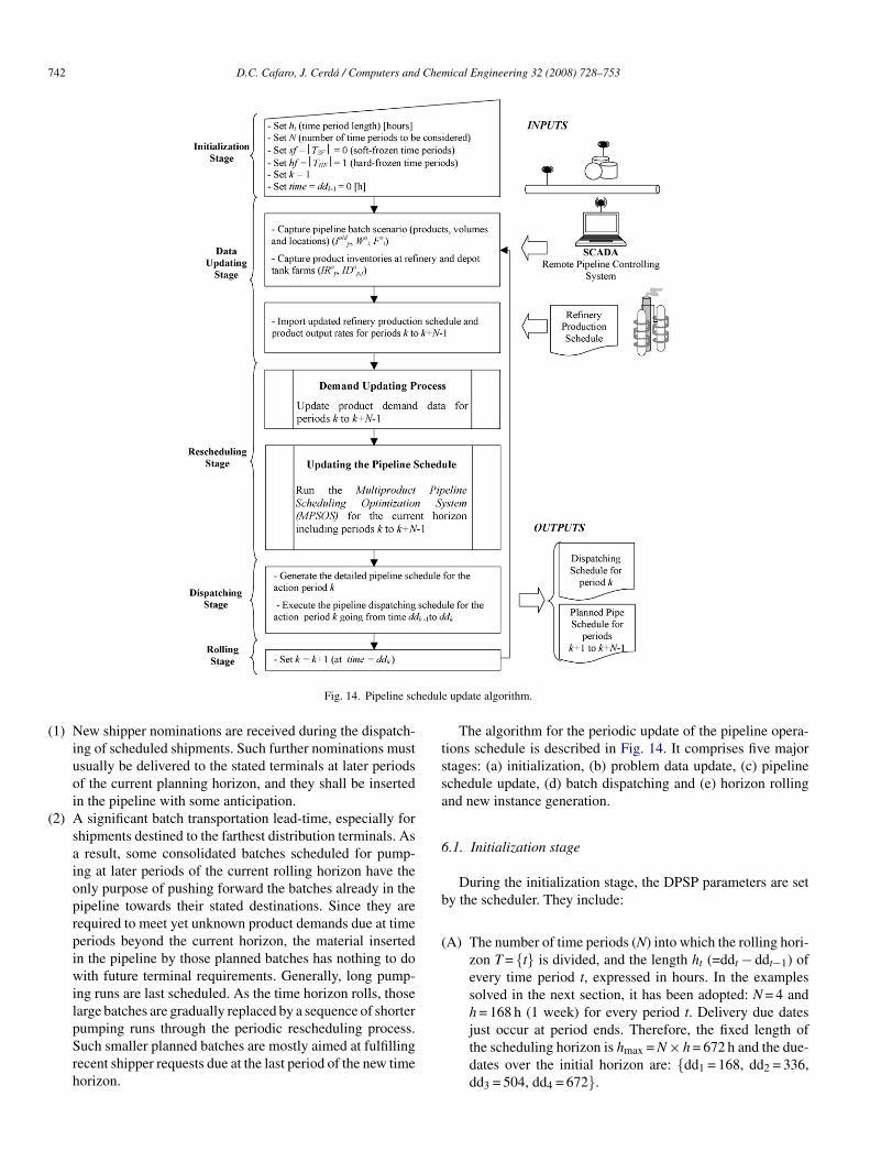
The algorithm for the periodic update of the pipeline opera-ions schedule is described in Fig. 14. It comprises five majortages: (a) initialization, (b) problem data update, (c) pipelinechedule update, (d) batch dispatching and (e) horizon rollingnd new instance generation.
.1. Initialization stage
During the initialization stage, the DPSP parameters are sety the scheduler. They include:
A) The number of time periods (N) into which the rolling hori-zon T = {t} is divided, and the length ht (=ddt − ddt−1) ofevery time period t, expressed in hours. In the examplessolved in the next section, it has been adopted: N = 4 and
just occur at period ends. Therefore, the fixed length ofthe scheduling horizon is hmax = N × h = 672 h and the due-dates over the initial horizon are: {dd1 = 168, dd2 = 336,dd3 = 504, dd4 = 672}.
Chem
(
(
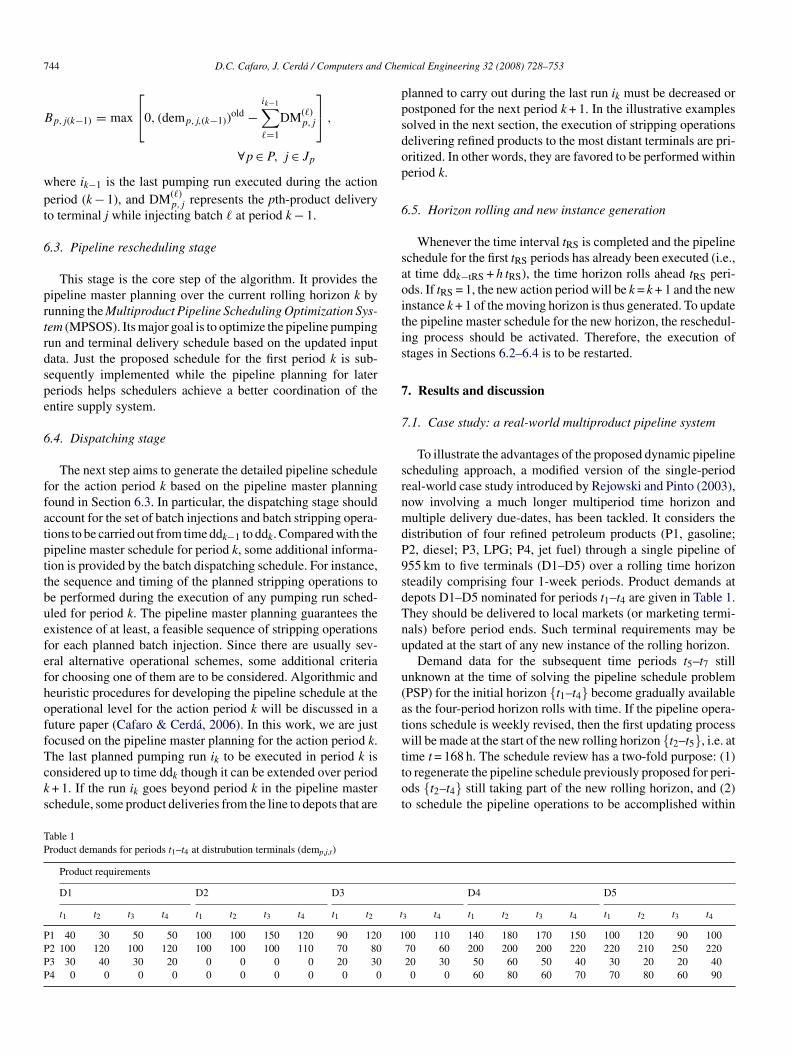
(
6
sipT
(
(
b
•
•
wtojock
D.C. Cafaro, J. Cerda / Computers and
(B) The number of different refined petroleum products tobe shipped from the refinery to the stated destinations,i.e. |P|.
(C) The number of consolidated new batches i ∈ Inew to bepumped in the pipeline along the multiperiod time horizon,i.e. the cardinality of the set Inew. The value of |Inew| is usu-ally set equal to: |Inew| = (N × |P|)/n, where n = 2.0 − 3.5. Ifthe adopted value for |Inew| is not large enough, the DPSPfeasible region may not include the true optimal sched-ule or, at worst, may be empty. Whenever the number ofnon-fictitious pumping runs NR at the optimum is equal to|Inew| or the DPSP is infeasible, the value of |Inew| must beincreased by one. After that, the DPSP is to be solved againuntil no improvement in the value of the objective functionis achieved.
D) The permissible ranges for product inventories at refin-ery and depot tankage (IRmin/IRmax, IDmin/IDmax), pipelinepump rates (vbmin/vbmax) and sent-to-market delivery rates(vmmax).
(E) The different types of pipeline operating unit costs arisingin the objective function as well as the product–productinterface size matrix.
(F) The time interval between two consecutive reviews of thepipeline schedule (tRS). This schedule regeneration fre-quency is expressed in time periods. In the examples solvedin this paper, tRS = 1 and the pipeline rescheduling processis executed at the start of every time period. Fig. 14 alsoassumes tRS = 1.
G) The subset of hard-frozen time periods THF ⊂ T, usuallyincluding the first-period of the new rolling horizon, wherethe planned pipeline operations must remain unchangedeven during the periodic pipeline rescheduling process. Inpractice, the regeneration frequency is generally equal to thenumber of hard frozen periods (tRS = |THF|). The illustrativeexamples solved in the next section and Fig. 14 assumetRS = |THF| = 1.
H) The subset of soft-frozen time periods TSF ⊂ T, usuallyincluding one or two periods immediately after the firstone, over which the sequence of planned product injectionscannot be modified. However, their pumping run lengthsmay be changed. In the examples solved in the next section:TSF = Ø.
(I) The subset of non-frozen time periods TNF = T −THF − TSF, where the pipeline schedule can be completelyreviewed.
(J) The first-period of the current moving horizon. Let us callit period k. The action period k will be used to identify thecorresponding instance of the moving horizon as it rollsover time. Set k = 1 for the initial horizon.
.2. Data updating stage
When the rescheduling process is activated or the pipeline
chedule for the initial horizon is to be generated, the next stages to update the input data for the current horizon k. Usually, theipeline schedule for the previous time horizon k − 1 is available.his stage involves the following steps:A
ical Engineering 32 (2008) 728–753 743
A) Capture the pipeline current status from the SCADA remotesystem to establish the sequence of batches in transit (Iold),i.e. batch naming (i), product (pi), size (Wo
i ) and location(Fo
i ). The SCADA remote system is usually available inevery multiproduct pipeline network.
(B) Pick up product inventory levels at refinery and terminaltank farms (IRo
p, IDop,j) at the start of the current horizon k
from the SCADA system, i.e. at time ddk−1.(C) Import the updated refinery production schedule and prod-
uct output rates for periods k to k + N − 1, i.e. fromtime = ddk−1 to time = ddk−1 + hmax. In most cases, therefinery production schedule is previously defined basedon crude oil inventories, product expected demands andavailable production capacity.
D) Update product demands at distribution terminals, includ-ing old demands not yet satisfied and new/cancelledshipments received while executing the pipeline sched-ule for the action period of the previous horizon (k − 1).To update terminal demands demp,j,t it must be taken intoaccount:(1) product deliveries to terminals accomplished during
period (k − 1) in advance of the promised time periodt > k − 1, ADp,j,t;
(2) product deliveries with due date ddk−1 that were notsatisfied during period k − 1 (backorders) and must befulfilled on the next action period k, Bp,j,(k−1).
Therefore, the updated terminal demands demp,j,t are giveny:
- For time period t = k,
demp,j,t = (demp,j,t)old + NSp,j,t − CSp,j,t
+ Bp,j,t−1 − ADp,j,t, ∀p ∈ P, j ∈ Jp
For time periods k + 1 ≤ t ≤ k + N − 2,
demp,j,t = (demp,j,t)old + NSp,j,t − CSp,j,t − ADp,j,t,
∀p ∈ P, j ∈ Jp
For time period t = k + N − 1 just incorporated in the rollinghorizon,
demp,j,t = NSp,j,t, ∀p ∈ P, j ∈ Jp
here (demp,j,t)old denotes terminal demand data available atime ddk−1 and the parameters NSp,j,t/CSp,j,t stand for the sizesf new/cancelled pth-product shipment nominations for terminaland period t received during period k − 1. Moreover, the sizesf anticipated product deliveries ADp,j,t and backorders Bp,j,k−1an be computed from the batch dispatching schedule for period− 1 through the following equations,⎡ ⎤
Dp,j,t = max⎣0,ik−1∑�=1
DM(�)p,j −
t∑n=k−1
(demp,j,n)old⎦ ,
∀p ∈ P, j ∈ Jp, t = k, . . . , k + N − 1
7 Chem
B
wpt
6
prtrdspe
6
ffatpttbuefefhoffTcks
ppsdop
6
saoitis
7
7
srnmdP9sdTnu
u(atw
TP
PPPP
44 D.C. Cafaro, J. Cerda / Computers and
p,j(k−1) = max
⎡⎣0, (demp,j,(k−1))
old −ik−1∑�=1
DM(�)p,j
⎤⎦ ,
∀p ∈ P, j ∈ Jp
here ik−1 is the last pumping run executed during the actioneriod (k − 1), and DM(�)
p,j represents the pth-product deliveryo terminal j while injecting batch � at period k − 1.
.3. Pipeline rescheduling stage
This stage is the core step of the algorithm. It provides theipeline master planning over the current rolling horizon k byunning the Multiproduct Pipeline Scheduling Optimization Sys-em (MPSOS). Its major goal is to optimize the pipeline pumpingun and terminal delivery schedule based on the updated inputata. Just the proposed schedule for the first period k is sub-equently implemented while the pipeline planning for latereriods helps schedulers achieve a better coordination of thentire supply system.
.4. Dispatching stage
The next step aims to generate the detailed pipeline scheduleor the action period k based on the pipeline master planningound in Section 6.3. In particular, the dispatching stage shouldccount for the set of batch injections and batch stripping opera-ions to be carried out from time ddk−1 to ddk. Compared with theipeline master schedule for period k, some additional informa-ion is provided by the batch dispatching schedule. For instance,he sequence and timing of the planned stripping operations toe performed during the execution of any pumping run sched-led for period k. The pipeline master planning guarantees thexistence of at least, a feasible sequence of stripping operationsor each planned batch injection. Since there are usually sev-ral alternative operational schemes, some additional criteriaor choosing one of them are to be considered. Algorithmic andeuristic procedures for developing the pipeline schedule at theperational level for the action period k will be discussed in auture paper (Cafaro & Cerda, 2006). In this work, we are justocused on the pipeline master planning for the action period k.
he last planned pumping run ik to be executed in period k isonsidered up to time ddk though it can be extended over period+ 1. If the run ik goes beyond period k in the pipeline masterchedule, some product deliveries from the line to depots that arettot
able 1roduct demands for periods t1–t4 at distrubution terminals (demp,j,t)
Product requirements
D1 D2 D3
t1 t2 t3 t4 t1 t2 t3 t4 t1 t2 t
1 40 30 50 50 100 100 150 120 90 120 12 100 120 100 120 100 100 100 110 70 803 30 40 30 20 0 0 0 0 20 304 0 0 0 0 0 0 0 0 0 0
ical Engineering 32 (2008) 728–753
lanned to carry out during the last run ik must be decreased orostponed for the next period k + 1. In the illustrative examplesolved in the next section, the execution of stripping operationselivering refined products to the most distant terminals are pri-ritized. In other words, they are favored to be performed withineriod k.
.5. Horizon rolling and new instance generation
Whenever the time interval tRS is completed and the pipelinechedule for the first tRS periods has already been executed (i.e.,t time ddk−tRS + h tRS), the time horizon rolls ahead tRS peri-ds. If tRS = 1, the new action period will be k = k + 1 and the newnstance k + 1 of the moving horizon is thus generated. To updatehe pipeline master schedule for the new horizon, the reschedul-ng process should be activated. Therefore, the execution oftages in Sections 6.2–6.4 is to be restarted.
. Results and discussion
.1. Case study: a real-world multiproduct pipeline system
To illustrate the advantages of the proposed dynamic pipelinecheduling approach, a modified version of the single-periodeal-world case study introduced by Rejowski and Pinto (2003),ow involving a much longer multiperiod time horizon andultiple delivery due-dates, has been tackled. It considers the
istribution of four refined petroleum products (P1, gasoline;2, diesel; P3, LPG; P4, jet fuel) through a single pipeline of55 km to five terminals (D1–D5) over a rolling time horizonteadily comprising four 1-week periods. Product demands atepots D1–D5 nominated for periods t1–t4 are given in Table 1.hey should be delivered to local markets (or marketing termi-als) before period ends. Such terminal requirements may bepdated at the start of any new instance of the rolling horizon.
Demand data for the subsequent time periods t5–t7 stillnknown at the time of solving the pipeline schedule problemPSP) for the initial horizon {t1–t4} become gradually availables the four-period horizon rolls with time. If the pipeline opera-ions schedule is weekly revised, then the first updating processill be made at the start of the new rolling horizon {t2–t5}, i.e. at
ime t = 168 h. The schedule review has a two-fold purpose: (1)o regenerate the pipeline schedule previously proposed for peri-ds {t2–t4} still taking part of the new rolling horizon, and (2)o schedule the pipeline operations to be accomplished within
D4 D5
3 t4 t1 t2 t3 t4 t1 t2 t3 t4
00 110 140 180 170 150 100 120 90 10070 60 200 200 200 220 220 210 250 22020 30 50 60 50 40 30 20 20 40
0 0 60 80 60 70 70 80 60 90
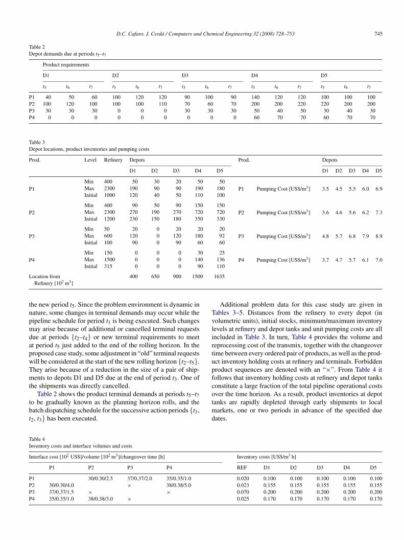
D.C. Cafaro, J. Cerda / Computers and Chemical Engineering 32 (2008) 728–753 745
Table 2Depot demands due at periods t5–t7
Product requirements
D1 D2 D3 D4 D5
t5 t6 t7 t5 t6 t7 t5 t6 t7 t5 t6 t7 t5 t6 t7
P1 40 50 60 100 120 120 90 100 90 140 120 120 100 100 100P2 100 120 100 100 100 110 70 60 70 200 200 220 220 200 200P3 30 30 30 0 0 0 30 30 30 50 40 50 30 40 30P4 0 0 0 0 0 0 0 0 0 60 70 70 60 70 70
Table 3Depot locations, product inventories and pumping costs
Prod. Level Refinery Depots Prod. Depots
D1 D2 D3 D4 D5 D1 D2 D3 D4 D5
P1Min 400 50 30 20 50 50
P1 Pumping Cost [US$/m3] 3.5 4.5 5.5 6.0 6.9Max 2300 190 90 90 190 180Initial 1000 120 40 50 110 100
P2Min 400 90 50 90 150 150
P2 Pumping Cost [US$/m3] 3.6 4.6 5.6 6.2 7.3Max 2300 270 190 270 720 720Initial 1200 230 150 180 350 330
P3Min 50 20 0 20 20 20
P3 Pumping Cost [US$/m3] 4.8 5.7 6.8 7.9 8.9Max 600 120 0 120 180 92Initial 100 90 0 90 60 60
P4Min 150 0 0 0 30 25
P4 Pumping Cost [US$/m3] 3.7 4.7 5.7 6.1 7.0Max 1500 0 0 0 140 136Initial 315 0 0 0 90 110
L 0
tnpmdapwTmt
tbt
Tvlirtupfc
TI
I
PPPP
ocation fromRefinery [102 m3]
400 650 900 150
he new period t5. Since the problem environment is dynamic inature, some changes in terminal demands may occur while theipeline schedule for period t1 is being executed. Such changesay arise because of additional or cancelled terminal requests
ue at periods {t2–t4} or new terminal requirements to meett period t5 just added to the end of the rolling horizon. In theroposed case study, some adjustment in “old” terminal requestsill be considered at the start of the new rolling horizon {t2–t5}.hey arise because of a reduction in the size of a pair of ship-ents to depots D1 and D5 due at the end of period t3. One of
he shipments was directly cancelled.
Table 2 shows the product terminal demands at periods t5–t7o be gradually known as the planning horizon rolls, and theatch dispatching schedule for the successive action periods {t1,
2, t3} has been executed.
otmd
able 4nventory costs and interface volumes and costs
nterface cost [102 US$]/volume [102 m3]/changeover time [h]
P1 P2 P3 P4
1 30/0.30/2.5 37/0.37/2.0 35/0.35/1.02 30/0.30/4.0 × 38/0.38/5.03 37/0.37/1.5 × ×4 35/0.35/1.0 38/0.38/3.0 ×
1635
Additional problem data for this case study are given inables 3–5. Distances from the refinery to every depot (inolumetric units), initial stocks, minimum/maximum inventoryevels at refinery and depot tanks and unit pumping costs are allncluded in Table 3. In turn, Table 4 provides the volume andeprocessing cost of the transmix, together with the changeoverime between every ordered pair of products, as well as the prod-ct inventory holding costs at refinery and terminals. Forbiddenroduct sequences are denoted with an “×”. From Table 4 itollows that inventory holding costs at refinery and depot tanksonstitute a large fraction of the total pipeline operational costs
ver the time horizon. As a result, product inventories at depotanks are rapidly depleted through early shipments to localarkets, one or two periods in advance of the specified dueates.
Inventory costs [US$/m3 h]
REF D1 D2 D3 D4 D5
0.020 0.100 0.100 0.100 0.100 0.1000.023 0.155 0.155 0.155 0.155 0.1550.070 0.200 0.200 0.200 0.200 0.2000.025 0.170 0.170 0.170 0.170 0.170
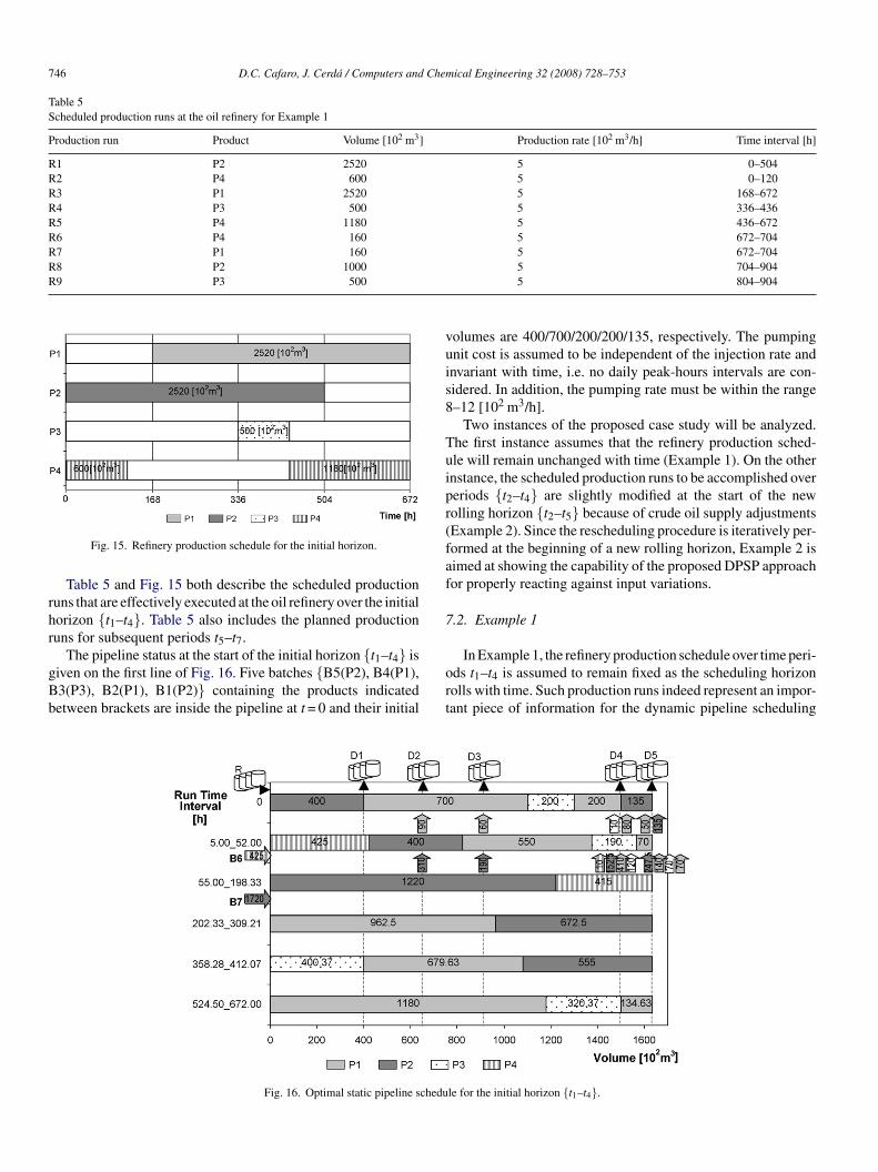
746 D.C. Cafaro, J. Cerda / Computers and Chemical Engineering 32 (2008) 728–753
Table 5Scheduled production runs at the oil refinery for Example 1
Production run Product Volume [102 m3] Production rate [102 m3/h] Time interval [h]
R1 P2 2520 5 0–504R2 P4 600 5 0–120R3 P1 2520 5 168–672R4 P3 500 5 336–436R5 P4 1180 5 436–672R6 P4 160 5 672–704R7 P1 160 5 672–704R8 P2 1000R9 P3 500
rhr
gBb
vuis8
Tuipr(faf
7
Fig. 15. Refinery production schedule for the initial horizon.
Table 5 and Fig. 15 both describe the scheduled productionuns that are effectively executed at the oil refinery over the initialorizon {t1–t4}. Table 5 also includes the planned productionuns for subsequent periods t5–t7.
The pipeline status at the start of the initial horizon {t1–t4} isiven on the first line of Fig. 16. Five batches {B5(P2), B4(P1),3(P3), B2(P1), B1(P2)} containing the products indicatedetween brackets are inside the pipeline at t = 0 and their initial
ort
Fig. 16. Optimal static pipeline schedu
5 704–9045 804–904
olumes are 400/700/200/200/135, respectively. The pumpingnit cost is assumed to be independent of the injection rate andnvariant with time, i.e. no daily peak-hours intervals are con-idered. In addition, the pumping rate must be within the range–12 [102 m3/h].
Two instances of the proposed case study will be analyzed.he first instance assumes that the refinery production sched-le will remain unchanged with time (Example 1). On the othernstance, the scheduled production runs to be accomplished overeriods {t2–t4} are slightly modified at the start of the newolling horizon {t2–t5} because of crude oil supply adjustmentsExample 2). Since the rescheduling procedure is iteratively per-ormed at the beginning of a new rolling horizon, Example 2 isimed at showing the capability of the proposed DPSP approachor properly reacting against input variations.
.2. Example 1
In Example 1, the refinery production schedule over time peri-ds t1–t4 is assumed to remain fixed as the scheduling horizonolls with time. Such production runs indeed represent an impor-ant piece of information for the dynamic pipeline scheduling
le for the initial horizon {t1–t4}.
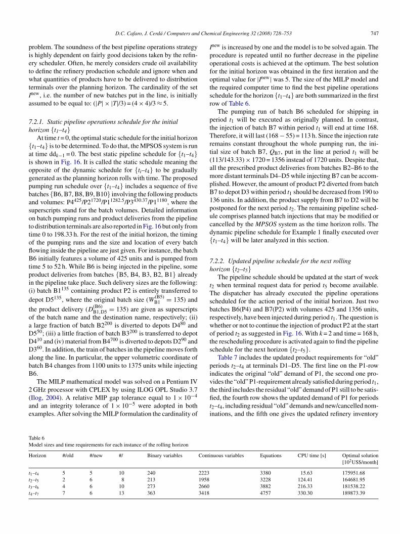
Chem
pietwtIa
7h
{aiogpbasottoflBtpi(d
toaDDDabB
2(ae
Ipofotsr
ptTrt(ampB1pucd{
7h
tTsbrwots
piv
TM
H
tttt
D.C. Cafaro, J. Cerda / Computers and
roblem. The soundness of the best pipeline operations strategys highly dependent on fairly good decisions taken by the refin-ry scheduler. Often, he merely considers crude oil availabilityo define the refinery production schedule and ignore when andhat quantities of products have to be delivered to distribution
erminals over the planning horizon. The cardinality of the setnew, i.e. the number of new batches put in the line, is initiallyssumed to be equal to: (|P| × |T|/3) = (4 × 4)/3 ≈ 5.
.2.1. Static pipeline operations schedule for the initialorizon {t1–t4}
At time t = 0, the optimal static schedule for the initial horizont1–t4} is to be determined. To do that, the MPSOS system is runt time ddk−1 = 0. The best static pipeline schedule for {t1–t4}s shown in Fig. 16. It is called the static schedule meaning thepposite of the dynamic schedule for {ti–t4} to be graduallyenerated as the planning horizon rolls with time. The proposedumping run schedule over {t1–t4} includes a sequence of fiveatches {B6, B7, B8, B9, B10} involving the following productsnd volumes: P4425/P21720/P11282.5/P3430.37/P11180, where theuperscripts stand for the batch volumes. Detailed informationn batch pumping runs and product deliveries from the pipelineo distribution terminals are also reported in Fig. 16 but only fromime 0 to 198.33 h. For the rest of the initial horizon, the timingf the pumping runs and the size and location of every batchowing inside the pipeline are just given. For instance, the batch6 initially features a volume of 425 units and is pumped from
ime 5 to 52 h. While B6 is being injected in the pipeline, someroduct deliveries from batches {B5, B4, B3, B2, B1} alreadyn the pipeline take place. Such delivery sizes are the following:i) batch B1135 containing product P2 is entirely transferred toepot D5135, where the original batch size (W (B5)
B1 = 135) and
he product delivery (D(B6)B1,D5 = 135) are given as superscripts
f the batch name and the destination name, respectively; (ii)large fraction of batch B2200 is diverted to depots D480 and550; (iii) a little fraction of batch B3200 is transferred to depot410 and (iv) material from B4700 is diverted to depots D290 and360. In addition, the train of batches in the pipeline moves forth
long the line. In particular, the upper volumetric coordinate ofatch B4 changes from 1100 units to 1375 units while injecting6.
The MILP mathematical model was solved on a Pentium IV
GHz processor with CPLEX by using ILOG OPL Studio 3.7Ilog, 2004). A relative MIP gap tolerance equal to 1 × 10⁻⁴
nd an integrity tolerance of 1 × 10⁻⁵ were adopted in bothxamples. After solving the MILP formulation the cardinality of
tfiti
able 6odel sizes and time requirements for each instance of the rolling horizon
orizon #/old #/new #/ Binary variables Conti
1–t4 5 5 10 240 2223
2–t5 2 6 8 213 1958
3–t6 4 6 10 273 2660
4–t7 7 6 13 363 3418
ical Engineering 32 (2008) 728–753 747
new is increased by one and the model is to be solved again. Therocedure is repeated until no further decrease in the pipelineperational costs is achieved at the optimum. The best solutionor the initial horizon was obtained in the first iteration and theptimal value for |Inew| was 5. The size of the MILP model andhe required computer time to find the best pipeline operationschedule for the horizon {t1–t4} are both summarized in the firstow of Table 6.
The pumping run of batch B6 scheduled for shipping ineriod t1 will be executed as originally planned. In contrast,he injection of batch B7 within period t1 will end at time 168.herefore, it will last (168 − 55) = 113 h. Since the injection rate
emains constant throughout the whole pumping run, the ini-ial size of batch B7, QB7, put in the line at period t1 will be113/143.33) × 1720 = 1356 instead of 1720 units. Despite that,ll the prescribed product deliveries from batches B2–B6 to theore distant terminals D4–D5 while injecting B7 can be accom-
lished. However, the amount of product P2 diverted from batch7 to depot D3 within period t1 should be decreased from 190 to36 units. In addition, the product supply from B7 to D2 will beostponed for the next period t2. The remaining pipeline sched-le comprises planned batch injections that may be modified orancelled by the MPSOS system as the time horizon rolls. Theynamic pipeline schedule for Example 1 finally executed overt1–t4} will be later analyzed in this section.
.2.2. Updated pipeline schedule for the next rollingorizon {t2–t5}
The pipeline schedule should be updated at the start of week2 when terminal request data for period t5 become available.he dispatcher has already executed the pipeline operationscheduled for the action period of the initial horizon. Just twoatches B6(P4) and B7(P2) with volumes 425 and 1356 units,espectively, have been injected during period t1. The question ishether or not to continue the injection of product P2 at the startf period t2 as suggested in Fig. 16. With k = 2 and time = 168 h,he rescheduling procedure is activated again to find the pipelinechedule for the next horizon {t2–t5}.
Table 7 includes the updated product requirements for “old”eriods t2–t4 at terminals D1–D5. The first line on the P1-rowndicates the original “old” demand of P1, the second one pro-ides the “old” P1-requirement already satisfied during period t1,
he third includes the residual “old” demand of P1 still to be satis-ed, the fourth row shows the updated demand of P1 for periods2–t4, including residual “old” demands and new/cancelled nom-nations, and the fifth one gives the updated refinery inventory
nuous variables Equations CPU time [s] Optimal solution[102US$/month]
3380 15.63 175951.683228 124.41 164681.953882 216.33 181538.224757 330.30 189873.39
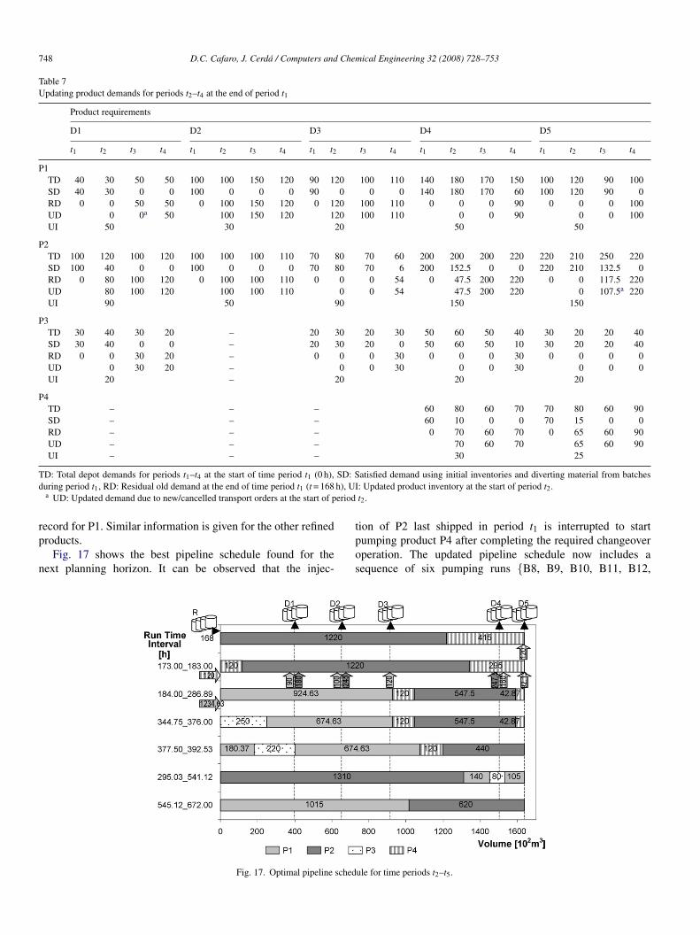
748 D.C. Cafaro, J. Cerda / Computers and Chemical Engineering 32 (2008) 728–753
Table 7Updating product demands for periods t2–t4 at the end of period t1
Product requirements
D1 D2 D3 D4 D5
t1 t2 t3 t4 t1 t2 t3 t4 t1 t2 t3 t4 t1 t2 t3 t4 t1 t2 t3 t4
P1TD 40 30 50 50 100 100 150 120 90 120 100 110 140 180 170 150 100 120 90 100SD 40 30 0 0 100 0 0 0 90 0 0 0 140 180 170 60 100 120 90 0RD 0 0 50 50 0 100 150 120 0 120 100 110 0 0 0 90 0 0 0 100UD 0 0a 50 100 150 120 120 100 110 0 0 90 0 0 100UI 50 30 20 50 50
P2TD 100 120 100 120 100 100 100 110 70 80 70 60 200 200 200 220 220 210 250 220SD 100 40 0 0 100 0 0 0 70 80 70 6 200 152.5 0 0 220 210 132.5 0RD 0 80 100 120 0 100 100 110 0 0 0 54 0 47.5 200 220 0 0 117.5 220UD 80 100 120 100 100 110 0 0 54 47.5 200 220 0 107.5a 220UI 90 50 90 150 150
P3TD 30 40 30 20 – 20 30 20 30 50 60 50 40 30 20 20 40SD 30 40 0 0 – 20 30 20 0 50 60 50 10 30 20 20 40RD 0 0 30 20 – 0 0 0 30 0 0 0 30 0 0 0 0UD 0 30 20 – 0 0 30 0 0 30 0 0 0UI 20 – 20 20 20
P4TD – – – 60 80 60 70 70 80 60 90SD – – – 60 10 0 0 70 15 0 0RD – – – 0 70 60 70 0 65 60 90UD – – – 70 60 70 65 60 90UI – – – 30 25
T SD: Sd h), UI
eriod
rp
n
D: Total depot demands for periods t1–t4 at the start of time period t1 (0 h),uring period t1, RD: Residual old demand at the end of time period t1 (t = 168a UD: Updated demand due to new/cancelled transport orders at the start of p
ecord for P1. Similar information is given for the other refinedroducts.
Fig. 17 shows the best pipeline schedule found for theext planning horizon. It can be observed that the injec-
tpos
Fig. 17. Optimal pipeline sched
atisfied demand using initial inventories and diverting material from batches: Updated product inventory at the start of period t2.t2.
ion of P2 last shipped in period t1 is interrupted to startumping product P4 after completing the required changeoverperation. The updated pipeline schedule now includes aequence of six pumping runs {B8, B9, B10, B11, B12,
ule for time periods t2–t5.
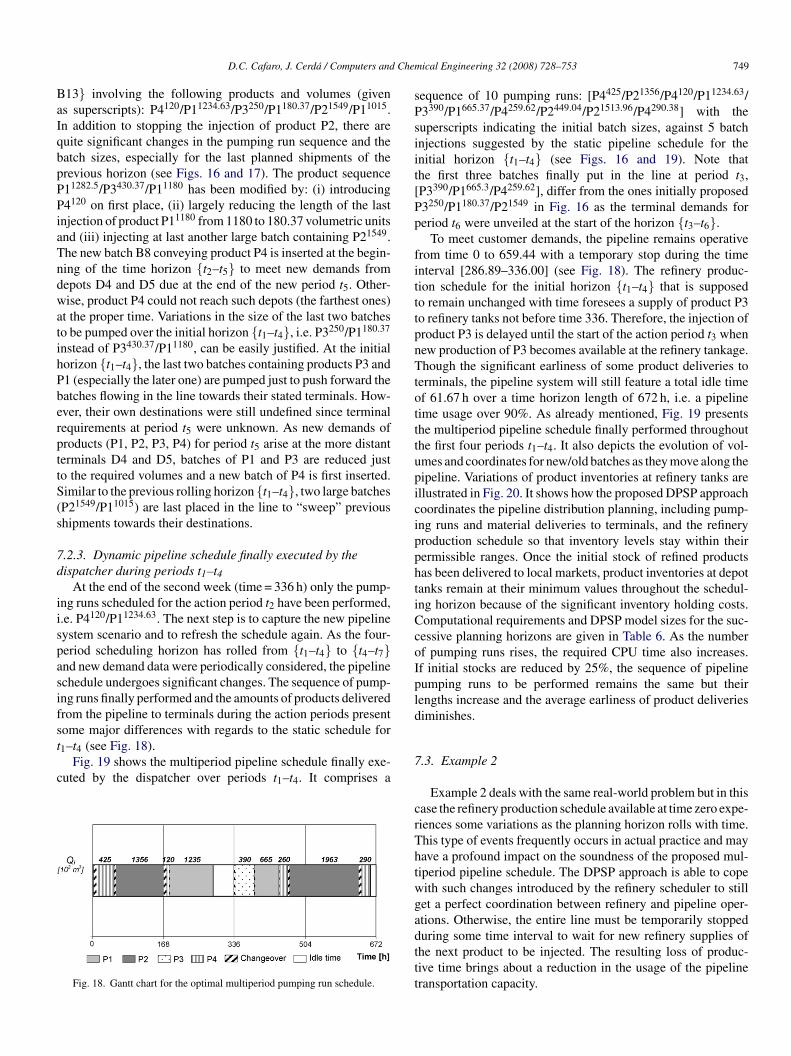
Chem
BaIqbpPPiaTndwatihPberpttS(s
7d
iispasifst
c
sPsiit[Pp
fitttpnTtotttupicipphtiCcoIpld
D.C. Cafaro, J. Cerda / Computers and
13} involving the following products and volumes (givens superscripts): P4120/P11234.63/P3250/P1180.37/P21549/P11015.n addition to stopping the injection of product P2, there areuite significant changes in the pumping run sequence and theatch sizes, especially for the last planned shipments of therevious horizon (see Figs. 16 and 17). The product sequence11282.5/P3430.37/P11180 has been modified by: (i) introducing4120 on first place, (ii) largely reducing the length of the last
njection of product P11180 from 1180 to 180.37 volumetric unitsnd (iii) injecting at last another large batch containing P21549.he new batch B8 conveying product P4 is inserted at the begin-ing of the time horizon {t2–t5} to meet new demands fromepots D4 and D5 due at the end of the new period t5. Other-ise, product P4 could not reach such depots (the farthest ones)
t the proper time. Variations in the size of the last two batcheso be pumped over the initial horizon {t1–t4}, i.e. P3250/P1180.37
nstead of P3430.37/P11180, can be easily justified. At the initialorizon {t1–t4}, the last two batches containing products P3 and1 (especially the later one) are pumped just to push forward theatches flowing in the line towards their stated terminals. How-ver, their own destinations were still undefined since terminalequirements at period t5 were unknown. As new demands ofroducts (P1, P2, P3, P4) for period t5 arise at the more distanterminals D4 and D5, batches of P1 and P3 are reduced justo the required volumes and a new batch of P4 is first inserted.imilar to the previous rolling horizon {t1–t4}, two large batchesP21549/P11015) are last placed in the line to “sweep” previoushipments towards their destinations.
.2.3. Dynamic pipeline schedule finally executed by theispatcher during periods t1–t4
At the end of the second week (time = 336 h) only the pump-ng runs scheduled for the action period t2 have been performed,.e. P4120/P11234.63. The next step is to capture the new pipelineystem scenario and to refresh the schedule again. As the four-eriod scheduling horizon has rolled from {t1–t4} to {t4–t7}nd new demand data were periodically considered, the pipelinechedule undergoes significant changes. The sequence of pump-ng runs finally performed and the amounts of products deliveredrom the pipeline to terminals during the action periods present
ome major differences with regards to the static schedule for1–t4 (see Fig. 18).Fig. 19 shows the multiperiod pipeline schedule finally exe-uted by the dispatcher over periods t1–t4. It comprises a
Fig. 18. Gantt chart for the optimal multiperiod pumping run schedule.
7
crThtwgadttt
ical Engineering 32 (2008) 728–753 749
equence of 10 pumping runs: [P4425/P21356/P4120/P11234.63/3390/P1665.37/P4259.62/P2449.04/P21513.96/P4290.38] with theuperscripts indicating the initial batch sizes, against 5 batchnjections suggested by the static pipeline schedule for thenitial horizon {t1–t4} (see Figs. 16 and 19). Note thathe first three batches finally put in the line at period t3,P3390/P1665.3/P4259.62], differ from the ones initially proposed3250/P1180.37/P21549 in Fig. 16 as the terminal demands foreriod t6 were unveiled at the start of the horizon {t3–t6}.
To meet customer demands, the pipeline remains operativerom time 0 to 659.44 with a temporary stop during the timenterval [286.89–336.00] (see Fig. 18). The refinery produc-ion schedule for the initial horizon {t1–t4} that is supposedo remain unchanged with time foresees a supply of product P3o refinery tanks not before time 336. Therefore, the injection ofroduct P3 is delayed until the start of the action period t3 whenew production of P3 becomes available at the refinery tankage.hough the significant earliness of some product deliveries to
erminals, the pipeline system will still feature a total idle timef 61.67 h over a time horizon length of 672 h, i.e. a pipelineime usage over 90%. As already mentioned, Fig. 19 presentshe multiperiod pipeline schedule finally performed throughouthe first four periods t1–t4. It also depicts the evolution of vol-mes and coordinates for new/old batches as they move along theipeline. Variations of product inventories at refinery tanks arellustrated in Fig. 20. It shows how the proposed DPSP approachoordinates the pipeline distribution planning, including pump-ng runs and material deliveries to terminals, and the refineryroduction schedule so that inventory levels stay within theirermissible ranges. Once the initial stock of refined productsas been delivered to local markets, product inventories at depotanks remain at their minimum values throughout the schedul-ng horizon because of the significant inventory holding costs.omputational requirements and DPSP model sizes for the suc-essive planning horizons are given in Table 6. As the numberf pumping runs rises, the required CPU time also increases.f initial stocks are reduced by 25%, the sequence of pipelineumping runs to be performed remains the same but theirengths increase and the average earliness of product deliveriesiminishes.
.3. Example 2
Example 2 deals with the same real-world problem but in thisase the refinery production schedule available at time zero expe-iences some variations as the planning horizon rolls with time.his type of events frequently occurs in actual practice and mayave a profound impact on the soundness of the proposed mul-iperiod pipeline schedule. The DPSP approach is able to copeith such changes introduced by the refinery scheduler to stillet a perfect coordination between refinery and pipeline oper-
tions. Otherwise, the entire line must be temporarily stoppeduring some time interval to wait for new refinery supplies ofhe next product to be injected. The resulting loss of produc-ive time brings about a reduction in the usage of the pipelineransportation capacity.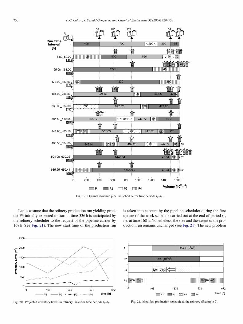
750 D.C. Cafaro, J. Cerda / Computers and Chemical Engineering 32 (2008) 728–753
line s
ut1
F
i
Fig. 19. Optimal dynamic pipe
Let us assume that the refinery production run yielding prod-
ct P3 initially expected to start at time 336 h is anticipated byhe refinery scheduler to the request of the pipeline carrier by68 h (see Fig. 21). The new start time of the production runig. 20. Projected inventory levels in refinery tanks for time periods t1–t4.
uid
chedule for time periods t1–t4.
s taken into account by the pipeline scheduler during the first
pdate of the work schedule carried out at the end of period t1,.e. at time 168 h. Nonetheless, the size and the extent of the pro-uction run remains unchanged (see Fig. 21). The new problemFig. 21. Modified production schedule at the refinery (Example 2).
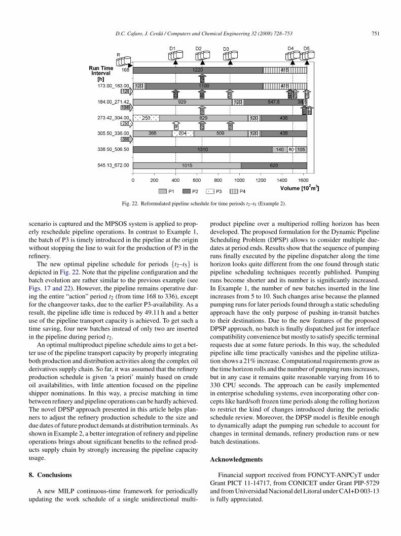
D.C. Cafaro, J. Cerda / Computers and Chemical Engineering 32 (2008) 728–753 751
dule
setwr
dbFifruti
tbdposbTndsouu
8
u
pdSdrhprIipatDcrpttb3ictstcb
A
Fig. 22. Reformulated pipeline sche
cenario is captured and the MPSOS system is applied to prop-rly reschedule pipeline operations. In contrast to Example 1,he batch of P3 is timely introduced in the pipeline at the originithout stopping the line to wait for the production of P3 in the
efinery.The new optimal pipeline schedule for periods {t2–t5} is
epicted in Fig. 22. Note that the pipeline configuration and theatch evolution are rather similar to the previous example (seeigs. 17 and 22). However, the pipeline remains operative dur-
ng the entire “action” period t2 (from time 168 to 336), exceptor the changeover tasks, due to the earlier P3-availability. As aesult, the pipeline idle time is reduced by 49.11 h and a betterse of the pipeline transport capacity is achieved. To get such aime saving, four new batches instead of only two are insertedn the pipeline during period t2.
An optimal multiproduct pipeline schedule aims to get a bet-er use of the pipeline transport capacity by properly integratingoth production and distribution activities along the complex oilerivatives supply chain. So far, it was assumed that the refineryroduction schedule is given ‘a priori’ mainly based on crudeil availabilities, with little attention focused on the pipelinehipper nominations. In this way, a precise matching in timeetween refinery and pipeline operations can be hardly achieved.he novel DPSP approach presented in this article helps plan-ers to adjust the refinery production schedule to the size andue dates of future product demands at distribution terminals. Ashown in Example 2, a better integration of refinery and pipelineperations brings about significant benefits to the refined prod-cts supply chain by strongly increasing the pipeline capacitysage.
. Conclusions
A new MILP continuous-time framework for periodicallypdating the work schedule of a single unidirectional multi-
Gai
for time periods t2–t5 (Example 2).
roduct pipeline over a multiperiod rolling horizon has beeneveloped. The proposed formulation for the Dynamic Pipelinecheduling Problem (DPSP) allows to consider multiple due-ates at period ends. Results show that the sequence of pumpinguns finally executed by the pipeline dispatcher along the timeorizon looks quite different from the one found through staticipeline scheduling techniques recently published. Pumpinguns become shorter and its number is significantly increased.n Example 1, the number of new batches inserted in the linencreases from 5 to 10. Such changes arise because the plannedumping runs for later periods found through a static schedulingpproach have the only purpose of pushing in-transit batcheso their destinations. Due to the new features of the proposedPSP approach, no batch is finally dispatched just for interface
ompatibility convenience but mostly to satisfy specific terminalequests due at some future periods. In this way, the scheduledipeline idle time practically vanishes and the pipeline utiliza-ion shows a 21% increase. Computational requirements grow ashe time horizon rolls and the number of pumping runs increases,ut in any case it remains quite reasonable varying from 16 to30 CPU seconds. The approach can be easily implementedn enterprise scheduling systems, even incorporating other con-epts like hard/soft frozen time periods along the rolling horizono restrict the kind of changes introduced during the periodicchedule review. Moreover, the DPSP model is flexible enougho dynamically adapt the pumping run schedule to account forhanges in terminal demands, refinery production runs or newatch destinations.
cknowledgments
Financial support received from FONCYT-ANPCyT underrant PICT 11-14717, from CONICET under Grant PIP-5729
nd from Universidad Nacional del Litoral under CAI+D 003-13s fully appreciated.
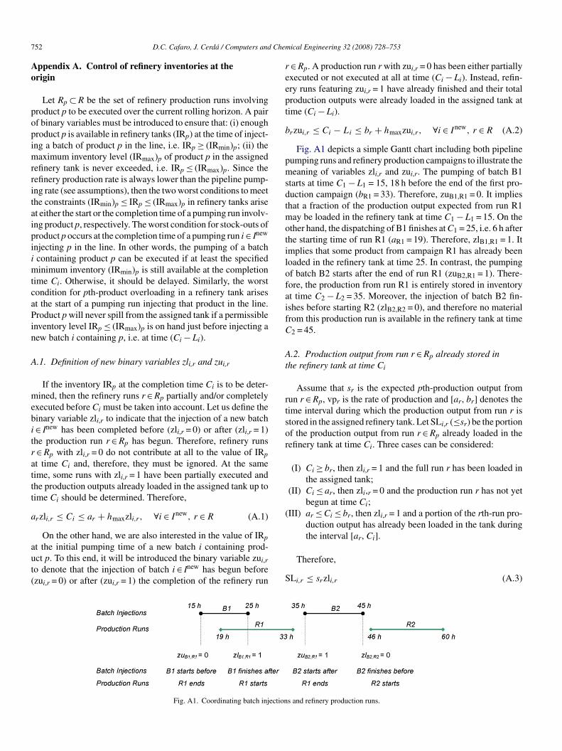
7 Chem
Ao
popimrritaipiimtcaPin
A
mebitrattt
a
aut(
reept
b
pmsdtmotilofaifC
At
rtsor
(
52 D.C. Cafaro, J. Cerda / Computers and
ppendix A. Control of refinery inventories at therigin
Let Rp ⊂ R be the set of refinery production runs involvingroduct p to be executed over the current rolling horizon. A pairf binary variables must be introduced to ensure that: (i) enoughroduct p is available in refinery tanks (IRp) at the time of inject-ng a batch of product p in the line, i.e. IRp ≥ (IRmin)p; (ii) the
aximum inventory level (IRmax)p of product p in the assignedefinery tank is never exceeded, i.e. IRp ≤ (IRmax)p. Since theefinery production rate is always lower than the pipeline pump-ng rate (see assumptions), then the two worst conditions to meethe constraints (IRmin)p ≤ IRp ≤ (IRmax)p in refinery tanks ariset either the start or the completion time of a pumping run involv-ng product p, respectively. The worst condition for stock-outs ofroduct p occurs at the completion time of a pumping run i ∈ Inew
njecting p in the line. In other words, the pumping of a batchcontaining product p can be executed if at least the specifiedinimum inventory (IRmin)p is still available at the completion
ime Ci. Otherwise, it should be delayed. Similarly, the worstondition for pth-product overloading in a refinery tank arisest the start of a pumping run injecting that product in the line.roduct p will never spill from the assigned tank if a permissible
nventory level IRp ≤ (IRmax)p is on hand just before injecting aew batch i containing p, i.e. at time (Ci − Li).
.1. Definition of new binary variables zli,r and zui,r
If the inventory IRp at the completion time Ci is to be deter-ined, then the refinery runs r ∈ Rp partially and/or completely
xecuted before Ci must be taken into account. Let us define theinary variable zli,r to indicate that the injection of a new batch∈ Inew has been completed before (zli,r = 0) or after (zli,r = 1)he production run r ∈ Rp has begun. Therefore, refinery runs∈ Rp with zli,r = 0 do not contribute at all to the value of IRp
t time Ci and, therefore, they must be ignored. At the sameime, some runs with zli,r = 1 have been partially executed andhe production outputs already loaded in the assigned tank up toime Ci should be determined. Therefore,
rzli,r ≤ Ci ≤ ar + hmaxzli,r, ∀i ∈ Inew, r ∈ R (A.1)
On the other hand, we are also interested in the value of IRp
t the initial pumping time of a new batch i containing prod-ct p. To this end, it will be introduced the binary variable zui,ro denote that the injection of batch i ∈ Inew has begun beforezui,r = 0) or after (zui,r = 1) the completion of the refinery run S
Fig. A1. Coordinating batch injection
ical Engineering 32 (2008) 728–753
∈ Rp. A production run r with zui,r = 0 has been either partiallyxecuted or not executed at all at time (Ci − Li). Instead, refin-ry runs featuring zui,r = 1 have already finished and their totalroduction outputs were already loaded in the assigned tank atime (Ci − Li).
rzui,r ≤ Ci − Li ≤ br + hmaxzui,r, ∀i ∈ Inew, r ∈ R (A.2)
Fig. A1 depicts a simple Gantt chart including both pipelineumping runs and refinery production campaigns to illustrate theeaning of variables zli,r and zui,r. The pumping of batch B1
tarts at time C1 − L1 = 15, 18 h before the end of the first pro-uction campaign (bR1 = 33). Therefore, zuB1,R1 = 0. It implieshat a fraction of the production output expected from run R1
ay be loaded in the refinery tank at time C1 − L1 = 15. On thether hand, the dispatching of B1 finishes at C1 = 25, i.e. 6 h afterhe starting time of run R1 (aR1 = 19). Therefore, zlB1,R1 = 1. Itmplies that some product from campaign R1 has already beenoaded in the refinery tank at time 25. In contrast, the pumpingf batch B2 starts after the end of run R1 (zuB2,R1 = 1). There-ore, the production from run R1 is entirely stored in inventoryt time C2 − L2 = 35. Moreover, the injection of batch B2 fin-shes before starting R2 (zlB2,R2 = 0), and therefore no materialrom this production run is available in the refinery tank at time2 = 45.
.2. Production output from run r ∈ Rp already stored inhe refinery tank at time Ci
Assume that sr is the expected pth-production output fromun r ∈ Rp, vpr is the rate of production and [ar, br] denotes theime interval during which the production output from run r istored in the assigned refinery tank. Let SLi,r (≤sr) be the portionf the production output from run r ∈ Rp already loaded in theefinery tank at time Ci. Three cases can be considered:
(I) Ci ≥ br, then zli,r = 1 and the full run r has been loaded inthe assigned tank;
(II) Ci ≤ ar, then zli,r = 0 and the production run r has not yetbegun at time Ci;
III) ar ≤ Ci ≤ br, then zli,r = 1 and a portion of the rth-run pro-duction output has already been loaded in the tank duringthe interval [ar, Ci].
Therefore,
Li,r ≤ srzli,r (A.3)
s and refinery production runs.
Chem
S
St
At
a(c
(
S
otsva(Oadt
Ao
feppimp
r
w(etoipabs
Q
p
w
R
C
C
H
IM
N
R
R
R
S
D.C. Cafaro, J. Cerda / Computers and
Li,r ≤ vpr(Ci − arzli,r), ∀i ∈ Inew, r ∈ R (A.4)
Constraint (A.3) is binding for cases (I) and (II). In this way,Li,r = sr for case (I) and SLi,r = 0 for case (II). In turn, the equa-
ion (A.4) becomes active for case (III) and SLi,r = vpr(Ci − ar).
.3. Production output from run r ∈ Rp already loaded inhe refinery tank at time (Ci − Li)
Let SUi,r denote the amount of product p from run r ∈ Rp
lready loaded in the refinery tank at the starting timeCi − Li) of a new pumping run i ∈ Inew. Two cases can beonsidered:
(I) (Ci − Li) ≥ br, then zui,r = 1 and the whole production runr is already stored in the refinery tank at time (Ci − Li);
II) (Ci − Li) < br, then zui,r = 0 and either a portion of or thewhole production run r is still to be loaded in the assignedtank at time (Ci − Li).
Therefore,
Ui,r ≥ srzui,r (A.5)
SUi,r ≥ vpr[(Ci − Li) − ar − hmaxzui,r), ∀i ∈ Inew, r ∈ R
(A.6)
Since the worst condition for overloading in refinery tanksccurs at the start of a pumping run and the amount SUi,r con-ributes to the value of IRp, the model will tend to make SUi,r asmall as possible. This is why lower bounds are defined for thealue of SUi,r through constraints (A.5) and (A.6). If zui,r = 1nd run r has been entirely loaded in the refinery tank at timeCi − Li), then Eq. (A.5) prevents from reducing SUi,r below sr.therwise, constraint (A.5) becomes redundant. In case zui,r = 0
nd ar < Ci − Li < br, constraint (A.6) would force SUi,r to neverrop below vpr[(Ci − Li) − ar]. If zui,r = 1, constraint (A.6) turnso be redundant.
.4. Testing worst conditions for product shortages andverloadings
As explained before, the inventory level for product p isorced to never falling below the minimum level (IRmin)p at thend of every pumping run i ∈ Inew, i.e. IRF(i)
p . In addition, theth-inventory level is required to never exceed the maximum
ermissible level (IRmax)p at the starting time of a new pump-ng run i ∈ Inew, i.e. IRS(i)p . Therefore, the following constraintsust be included in the problem formulation to guarantee that the
th-product inventory level in the assigned refinery tank always
S
T
ical Engineering 32 (2008) 728–753 753
emains within the specified feasible range [(IRmin)p, (IRmax)p].
IRF(i)p = IRo
p +∑
r ∈ Rp
SLi,r −∑
i′ ∈ Inew,i′≤i
QPi′,p ≥ (IRmin)p,
∀i ∈ Inew, p ∈ P (A.7)
IRS(i)p = IRo
p +∑
r ∈ Rp
SUi,r −∑
i′ ∈ Inew,i′<i
QPi′,p ≤ (IRmax)p,
∀i ∈ Inew, p ∈ P (A.8)
here IRop stands for the initial inventory of product p. Constraint
A.7) accounts for pth-product supplies to inventory from refin-ry runs r ∈ Rp starting before time Ci. In addition, it considershe product withdrawals from refinery tanks related to batchesf product p injected in the pipeline up to Ci. Constraint (A.8)s similar to (A.7) but the referenced time point is now the startoint of a pumping run (Ci − Li) rather than Ci. Note that themount of product p injected in the line QPi′,p equals zero ifatch i′ does not contain p. Otherwise, it is equal to the initialize of batch i′ (Qi′ ). Therefore,
Pi,p ≤ Qmaxyi,p, ∀i ∈ Inew, p ∈ P (A.9)∑∈ P
QPi,p = Qi, ∀i ∈ Inew (A.10)
here Qmax stands for the maximum permissible injection size.
eferences
afaro, D. C., & Cerda, J. (2004). Computers and Chemical Engineering, 28,2053–2068.
afaro, D. C., & Cerda, J. (2006). Proceedings of XXII Interamerican Congressof Chemical Engineering.
ull, B. (2005). Oil pipeline markets and operations. Journal of the Transporta-tion Research Forum, 44, 111–125.
LOG OPL Studio 3.7 User’s Manual (2004). ILOG S.A: France.agatao, L., Arruda, L. V. R., & Neves, F., Jr. (2004). Computers and Chemical
Engineering, 28, 171–185.eiro, S. M. S., & Pinto, J. M. (2004). Computers and Chemical Engineering,
28, 871–896.abinow, R. A. (2004). The liquid pipeline industry in the United States, where
it’s been, where it’s going. Association of Oil Pipelines, (April).ejowski, R., & Pinto, J. M. (2003). Computers and Chemical Engineering, 27,
1229–1246.ejowski, R., & Pinto, J. M. (2004). Computers and Chemical Engineering, 28,
1511–1528.asikumar, M., Prakash, P. R., Patil, S. M., & Ramani, S. (1997). Knowledge-
Based Systems, 10, 169–175.
heppard, N. (1984). Introduction to the oil pipeline industry (3rd ed.). Austin,TX: University of Texas.rench, Ch. J. (2001). How pipelines make the oil market work—Their networks,
operation, and regulation. New York: Allegro Energy Group, Associationof Oil Pipe Lines., pp. 1–20 (December).