Dynamics and Stability of Variable-Length, Vertically-Traveling,Heavy Cables: Application to Tethered Aerostats

Dipayan Mukherjee,∗ Ishan Sharma,† and Shakti S. Gupta‡

Indian Institute of Technology Kanpur, Kanpur 208 016, Uttar Pradesh, India

DOI: 10.2514/1.C034931

The dynamics and stability of variable-length vertically traveling, heavy cables with an end load are investigated.

Such cables act as tethers in aerostat systems. The cable is modeled as a heavy string undergoing small, planar

vibrationswhile attached to a rigid, spherical aerostat.Aerodynamic andbuoyancy forces act only on the aerostat. An

asymptotic analysis for slow deployment rates provides excellent leading-order approximation to the dynamics,

which is also obtained from finite element simulations. Stability of the aerostat system is then investigated

computationally by considering the linear stability of the systemwhen it is perturbed from its nominal dynamical state

at any given time. It is found that, when an aerostat ascends, the cable always goes unstable after a certain time

through a divergence instability. In contrast, flutter instability is found in the cable during the aerostat’s descent.

These stability analyses help in thedevelopment of deployment charts that relate themaximumachievable elevation to

deployment rate. Such deployment charts can help in parameter selection for efficient aerostat deployment. The

dynamics of the aerostat in the presence of spatiotemporally varying aerodynamic forces are also studied

computationally. The paper concludeswith two case studies of aerostat deployment that demonstrate the utility of the

current analysis.

Nomenclature

A = cross-sectional area of the cable, m2

a, ~a = dimensional (ms−2) and nondimensionalacceleration of ascent/descent

�E, �EP, �EK = nondimensional total, potential, and kineticenergies associated with the system

Fb = buoyancy force on the aerostat, N�F = nondimensional net buoyancy force on the

aerostath = nondimensional elevation of the aerostatL, l = dimensional (m) and nondimensional

lengths of the cableM��t�, G��t�,K��t� = n × n global mass, gyroscopic, and stiff-

ness matrices of the systemm, ~m = dimensional (kg) and nondimensional

masses of the aerostatq��t� = n × 1 nodal displacements of the cableqend = end-tip (aerostat) deflectionq̂i = n × 1, ith eigenvector of the system at �t

equal to t̂r = radius the aerostat, mt, �t = dimensional (s) and nondimensional times�t� = nondimensional critical time after which

the system goes unstablev, ~v = dimensional (ms−1) and nondimensional

rates of ascent/descentx = position of a point on the cable, my�x; t�, ~y�ζ; t� = transverse deflections of the cable, mζ = position of a point on the aerostat in the

mapped domain; x∕Lη�ζ; �t� = nondimensional transverse deflection

λi = ith eigenvalue of the system at �t equal to t̂ρ = density of the cable, kg∕m−3

I. Introduction

A XIALLY translating continua with varying lengths gives riseto rich dynamics [1–7] and has important engineering and

aerospace applications. For example, vertically traveling heavycables that lengthen or shorten find applications as tethers of high-altitude balloons (aerostats); see, e.g., the work of Aglietti [8].Tethered aerostat systems have been studied by Jones and Krausman[9], Lambert and Nahon [10], Kang and Lee [11], Hembree andSlegers [12], and Mi and Gottlieb [13]. In all these studies. the focuswas on the deployed state when the tether’s length was fixed.Furthermore, all except Mi and Gottlieb [13] took the tether as acomposition of discrete elements, and they did not model it as acontinuum. Although the dynamics of variable-length tetheredsatellite systems was investigated by Mankala and Agrawal [14,15],no points weremade by the authors on the instability in such systems.In this paper, we investigate the dynamics and stability of variable-length vertically translating, heavy cables and apply it to study thedynamics and stability of ascending/descending tethered aerostats.Figure 1a shows a sketch of the aerostat system.Initial investigations on the spaghetti problem (i.e., an oscillating

cable that is shortening in length) were carried out by Carrier [1].Subsequently, Mansfield and Simmonds [2] investigated the dynamicsof a lengthening cable, issuing from an orifice, which the authorstermeda reversed spaghetti problem.Pesce [16] developed avariationalframework for the variable mass systems and investigated an exampleof the deployment of a heavy cable from a reel. The dynamics of ahorizontally deploying cable attached to an end mass has been studiedby Crellin et al. [17]. In all these works, the primary goal was toinvestigate the evolution of the spatial configuration of the tether intime, whereas no investigation on the instability has been reported. Thedynamics of axially lengthening/shortening beams and cables has beenstudied by Zhu and Ni [18] and Terumichi et al. [5] for application toelevator systems, and by Stylianou and Tabarrok [3] andGosselin et al.[6] in the context of extruding beams. A more involved geometricallynonlinear formulation of axially lengthening/shortening geometricallyexact beams was provided by Vu-Quoc and Li [19].Axially translating continua are susceptible to instabilities [6,20–22].

Instability in beams of periodically varying lengths has been studied byElmaraghy and Tabarrok [23], Zajaczkowski and Lipiński [24], andHyun andYoo [25]. In contrast, the change in the length of the tether ofan ascending/descending aerostat is monotonic. This monotonicity in

Received 23 January 2018; revision received 19 May 2018; accepted forpublication 21 May 2018; published online 12 September 2018. Copyright© 2018 by Ishan Sharma. Published by the American Institute of Aeronauticsand Astronautics, Inc., with permission. All requests for copying andpermission to reprint should be submitted to CCC at www.copyright.com;employ the ISSN 0021-8669 (print) or 1533-3868 (online) to initiate yourrequest. See also AIAA Rights and Permissions www.aiaa.org/randp.

*Masters Student, Department ofMechanical Engineering,Mechanics andApplied Mathematics Group; dipayan.me2010@gmail.com.

†Professor, Department ofMechanical Engineering,Mechanics and AppliedMathematics Group; ishans@iitk.ac.in (Corresponding Author).

‡Associate Professor, Department of Mechanical Engineering, Mechanicsand Applied Mathematics Group; ssgupta@iitk.ac.in.

68

JOURNAL OF AIRCRAFT

Vol. 56, No. 1, January–February 2019

Dow

nloa

ded

by I

ND

IAN

IN

STIT

UT

E O

F T

EC

HN

OL

OG

Y o

n O

ctob

er 2

7, 2

019

| http

://ar

c.ai

aa.o

rg |

DO

I: 1

0.25

14/1

.C03

4931

the variation of the cable’s length necessitates a quasi-static eigenvalueanalysis of the system, as employed by Stylianou and Tabarrok [4] andGosselin et al. [6]. Nawrotzki and Eller [26] used the quasi-staticeigenvalue analysis to investigate stability of nonlinear structures. Zhuand Ni [18] studied the stability of lengthening/shortening elevatorcables in light of evolution of the total mechanical energy of thesystem. However, it was shown by Yang and Mote [27] and Ziegler([28] pp. 36-40) that the evolution of energy could not be a measure ofthe stability of a dynamical system in the presence of gyroscopic terms,which typically arise in the study of travelling cables.Our mathematical model is as follows. We model the cable as a

tensioned, heavy string of varying length and the aerostat as a rigidsphere. As a first step, we restrict ourselves to small oscillations in aplane. Aerodynamic and buoyancy effects are considered on theaerostat alone. Our aerodynamic model, based on work by Tchen[29], Corrsin and Lumley [30], and Maxey and Riley [31], includesthe effects of the flow’s pressure gradient, Stokes drag, and addedmass, but it ignores vortex shedding. We analyze the dynamics ofthe aerostat system, both through an asymptotic analysis of areduced-order model and by a finite element analysis. The stability ofthe aerostat system during deployment is found to depend cruciallyon the stability of the lengthening/shortening cable (tether). Thisstability is investigated computationally following the quasi-staticlinear stability analysis mentioned previously. We find that allascending aerostats are susceptible to divergence instabilities,which limits the maximum elevation that can be achieved in terms ofits deployment rate. Descending aerostats, on the other hand,go unstable through a flutter instability. We note that we do notincorporate structural damping in the cable at present, and this leadsto a more conservative description of instability.This paper is organized as follows. In Sec. II, we derive the

equations ofmotion for ascending/descending aerostat systems usingboth linear momentum balance and variational principle. Asymptoticapproximations are employed to investigate the vibrations of aslowly ascending/descending aerostat system in Sec. III. Divergenceinstability in ascending aerostats is then demonstrated in Sec. IV.This instability is then investigated through an eigenvalue analysis.Instability in descending aerostats is studied in Sec. V. We theninvestigate the forced vibration of ascending/descending aerostatsystems under steady, temporally nonuniform air flow in Sec. VI.Finally, in Sec. VII, we conclude with two case studies of ascendingaerostats that demonstrate how we may use our results.

II. Equations of Motion

In this section, we summarize the equations of motion for a

lengthening/shortening cable, modeling it as a heavy, inextensible

string of varying length; the details of the derivation are in the

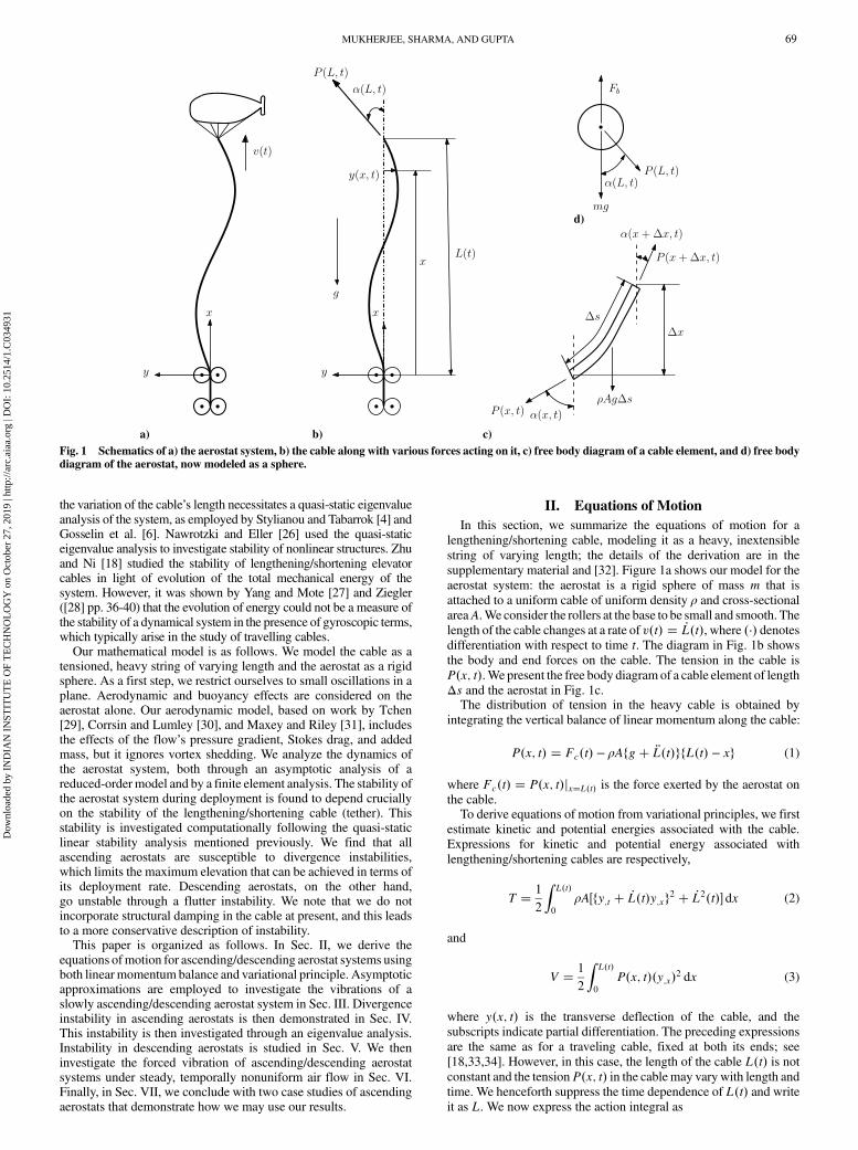
supplementary material and [32]. Figure 1a shows our model for the

aerostat system: the aerostat is a rigid sphere of mass m that is

attached to a uniform cable of uniform density ρ and cross-sectionalareaA.We consider the rollers at the base to be small and smooth. The

length of the cable changes at a rate of v�t� � _L�t�, where �⋅� denotesdifferentiation with respect to time t. The diagram in Fig. 1b shows

the body and end forces on the cable. The tension in the cable is

P�x; t�.We present the free body diagram of a cable element of length

Δs and the aerostat in Fig. 1c.The distribution of tension in the heavy cable is obtained by

integrating the vertical balance of linear momentum along the cable:

P�x; t� � Fc�t� − ρAfg� �L�t�gfL�t� − xg (1)

where Fc�t� � P�x; t�jx�L�t� is the force exerted by the aerostat on

the cable.To derive equations of motion from variational principles, we first

estimate kinetic and potential energies associated with the cable.

Expressions for kinetic and potential energy associated with

lengthening/shortening cables are respectively,

T � 1

2

ZL�t�

0

ρA�fy;t � _L�t�y;xg2 � _L2�t�� dx (2)

and

V � 1

2

ZL�t�

0

P�x; t��y;x�2 dx (3)

where y�x; t� is the transverse deflection of the cable, and the

subscripts indicate partial differentiation. The preceding expressions

are the same as for a traveling cable, fixed at both its ends; see

[18,33,34]. However, in this case, the length of the cable L�t� is notconstant and the tensionP�x; t� in the cable may vary with length and

time. We henceforth suppress the time dependence of L�t� and writeit as L. We now express the action integral as

c)

d)

b)a)Fig. 1 Schematics of a) the aerostat system, b) the cable along with various forces acting on it, c) free body diagram of a cable element, and d) free bodydiagram of the aerostat, now modeled as a sphere.

MUKHERJEE, SHARMA, AND GUPTA 69

Dow

nloa

ded

by I

ND

IAN

IN

STIT

UT

E O

F T

EC

HN

OL

OG

Y o

n O

ctob

er 2

7, 2

019

| http

://ar

c.ai

aa.o

rg |

DO

I: 1

0.25

14/1

.C03

4931

Zt2

t1

�δT − δV� dt � 0 (4)

where δ�⋅� is the variational operator.We note that the spatial domainof integration is changing with time. A direct attempt to deriveequations of motion from this may invite additional complexity. Toovercome this problem, we perform a change of variable [19,35]. Wetake ζ � x∕L such that 0 ≤ ζ ≤ 1. The transverse displacementbecomes ~y�ζ; t� � y�x; t�. Derivatives transform as

y;x � ~y;ζ∂ζ∂x

� ~y;ζL

; and y;t � ~y;t � ~y;ζ∂ζ∂t

� ~y;t − ~y;ζζ _L

L

The modified expressions for kinetic and potential energy are then

T � 1

2

Z1

0

ρAL

��~y;t � �1 − ζ� ~y;ζ

_L

L

�2

� _L2

�dζ (5)

and

V � 1

2

Z1

0

�Fc�t�L

− ρAfg� �L�t�g�1 − ζ��~y2;ζ dζ (6)

whereFc�t� � P�L; t� is the applied force at the free end of the cable.Substituting the preceding in Eq. (4) and integrating the result byparts, we obtain the governing equation for the aerostat system (seethe supplementary material for details):

ρAL ~y;tt�2ρA�1−ζ� _L ~y;ζt�ρA�1−ζ� �L ~y;ζ�ρA∂∂ζ

��1−ζ�2

�L2

L~y;ζ

�

� ∂∂ζ

��Fc

L−ρA�g� �L��1−ζ�

�~y;ζ

�(7)

and the geometric boundary condition at the roller (lower) end:

~y � 0 at ζ � 0 (8)

To obtain the natural boundary condition at the upper end of thecable and the expression for the force Fc on the cable, we balancevertical and horizontal forces on the aerostat attached to the cable atx � L; see Fig. 1d. We obtain, respectively,

Fc�t� � Fb −m�g� �L� ≕ F −m �L (9a)

and

m�y;tt�2y;xt _L�y;xx _L2�y;x �L��Fc�t�y;x � 0 at x�L (9b)

whereFb is the buoyancy force on the aerostat. Combining these twoequations and expressing in terms of ζ � x∕L yields

m

�~y;tt −

�L

L~y;ζ

�� F

L~y;ζ � 0 at ζ � 1 (10)

which represents the natural boundary condition for the system at theupper end of ζ � 1. We nondimensionalize Eq. (7) to find

lη;�t �t � 2�1 − ζ�_lη;ζ�t � �1 − ζ��lη;ζ �∂∂ζ

��1 − ζ�2

_l2

lη;ζ

�

� ∂∂ζ

��1

l− ~m

�l

l−�1

~F� �l

��1 − ζ�gη;ζ

�(11)

where the nondimensional deflection

η�ζ; �t� � ~y�ζ; t�∕L0

is defined in terms of initial length L0 of the cable, and thenondimensional time is

�t � t1

L0

������F

ρA

s

whereas the total derivative with respect to �t is again denoted by �⋅�,the nondimensional length of the cable is l��t� � L∕L0, the

nondimensional external force is ~F � F∕ρAgL0, and the nondimen-sional mass of the aerostat is ~m � m∕ρAL0. We define the

nondimensional velocity ~v � _l � _L������������ρA∕F

p, where

������������F∕ρA

pis the

speed of travelling waves in a string kept at a constant tension F.Finally, we define a nondimensional acceleration of

~a � �l � �LρA∕F. The boundary conditions [Eqs. (8) and (10)] arenondimensionalized as

η � 0 at ζ � 0 (12a)

and

~m

�η;�t �t −

�l

lη;ζ

�� 1

lη;ζ � 0 at ζ � 1 (12b)

The transverse vibrations of the lengthening/shortening cable aregoverned by the partial differential equation [Eq. (11)] alongwith theboundary conditions [Eq. (10)].Wemake two comments. The system does not preserve energy due

to a continuous supply/depletion of mass at the cable’s lower end.Thus, the system is non-Hamiltonian. We also note the presence ofthe gyroscopic term η;ξ�t in Eq. (11), which affects the stability of thesystem but does not contribute to the system’s kinetic energy. Thus,an energetic stability analysis will be incomplete because it willoverlook the role of such gyroscopic terms; see, e.g., the work ofZiegler ([28] pp. 36–40).

III. Slowly Lengthening/Shortening Cables

It is possible to make significant progress through the analysis of areduced-order model when the cable’s lengthening/shortening rate issmall. To develop a reduced-order model of the system, we expressthe deflection η�ζ; �t� as

η�ζ; �t� �Xni�0

Wi�ζ�qi��t�

whereWi�ζ� is the ith mode of vibration that satisfies the geometricboundary condition [Eq. (12a)], and qi��t� is the temporal evolution ofthemode. A reduced-order model is obtained by considering only thefirst mode, which is taken to be

W�ζ� � sin

�π

2ζ

�(13)

We replace the preceding approximation in the weighted residualform associated with Eq. (11) and the natural boundary condition[Eq. (12b)], and we follow Galerkin’s method; see the work ofHagedorn and Dasgupta ([36] pp. 47–49). Projection onto thefirst mode leads to a single-degree-of-freedom approximation ofEq. (11), viz.,

�2 ~m� l� �q��t�� _l _q��t���χ �l� κ

��l

l� 4

_l2

l2

�� α

l� β

_l2

l� γ

�q��t� � 0

(14)

where

α � π2

4; β � −

�1

2� π2

12

�; γ � −

1

~F

�π2

8� 1

2

�;

κ � −π2

4~m and χ �

�1

2−π2

8

�(15)

70 MUKHERJEE, SHARMA, AND GUPTA

Dow

nloa

ded

by I

ND

IAN

IN

STIT

UT

E O

F T

EC

HN

OL

OG

Y o

n O

ctob

er 2

7, 2

019

| http

://ar

c.ai

aa.o

rg |

DO

I: 1

0.25

14/1

.C03

4931

Wenow investigate the single-degree-of-freedommodel [Eq. (14)]through asymptotics.

A. Asymptotic Analysis

The time scale of transverse vibrations may be estimated from thefrequency of the first mode of a cable of fixed lengthL, and this yields

2L∕������������F∕ρA

p([36] pp. 47–49). This time scale, however, changes with

the cable’s length on a time scale L∕v associated with the deploymentrate v of the cable. For typical aerostat systems, the ratio of these two

time scales is v∕������������F∕ρA

p≪ 1, so that fast transverse vibrations are

modified slowly by the deployment rate. Indeed, for usual deployment

rates of v � 1.0–1.2 ms−1 [37,38] and representative values of

F�≈350 kN� and ρA�≈3.75 kg∕m−1�, we find that v∕ ������������F∕ρA

plies in

the range 0.002–0.005. We thus expect the system’s dynamics todisplay “slow” and “fast” time scales associated with, respectively, its

axial lengthening/shortening and its transverse vibrations.Given the preceding discussion, we express time as

�t � T � τ�O�ϵ2� (16)

where T � O��t�, τ � ϵ�t is the slow time scale; and 0 < ϵ ≪ 1 is asmall parameter introduced to aid the perturbation analysis. By our

assumption, l�T; τ� � l�τ�. It is shown in [32] that a regular multiplescale perturbation method fails for nonautonomous systems likeEq. (14). This drawback of the multiple scale method may beovercome through the Wentzel–Kramers–Brillouin (WKB) method;

see ([39] pp. 556–559) or ([40] pp. 127–129). In the WKB method,we assume q to be of the form

q � q�T�; τ; ϵ�

where T� ≠ T is a modified fast time, defined as T� � ϕ�τ�∕ϵ; thefunction ϕ�τ�will be defined later. The choice of ϕ�τ�must ensure aperiodic solution of q in T� so that q�T�; τ; ϵ� � q�2π � T�; τ; ϵ�.Employing the definitions of T� and τ and treating them asindependent quantities, the chain rule yields

d�⋅�d�t

� ∂ϕ�τ�∂τ

∂�⋅�∂T� � ϵ

∂�⋅�∂τ

(17a)

and

d2�⋅�d�t2

��∂ϕ�τ�∂τ

�2 ∂2�⋅�∂T�2�ϵ

�2∂ϕ�τ�∂τ

∂2�⋅�∂T�∂τ

�∂2ϕ�τ�∂τ2

∂�⋅�∂T�

��ϵ2

∂2�⋅�∂τ2

(17b)

Expanding temporal derivatives in Eq. (14) as shown earlier andcollecting O�1� terms, we obtain�

∂ϕ�τ�∂τ

�2 ∂2q0�T�; τ�

∂T�2 � ψ�τ�2q0�T�; τ� � 0 (18)

where

ψ�τ� ��

α

l�τ�f2 ~m� l�τ�g �γ

2 ~m� l�τ���1∕2�

We now define

ϕ�τ� �Z

τ

0

ψ�τ� dτ

so that ∂ϕ�τ�∕∂τ � ψ�τ�, and this simplifies Eq. (18).With this, the general solution of Eq. (18) is obtained as

q0�T�; τ� � A0�τ�eiT� � �A0�τ�e−iT�

To obtain A0�τ�, we collect O�ϵ� terms from Eq. (14) after

expanding its temporal derivatives through Eq. (12) to find

∂2q1�T�;τ�∂T�2 �q1�T�;τ�� 2

ψ�τ�∂2q0�T�;τ�

∂T�∂τ� 1

ψ�τ�2∂ψ�τ�∂τ

∂q0�T�;τ�∂T�

� 1

ψ�τ�f2 ~m� l�τ�gdl�τ�dτ

∂q0�T�;τ�∂T� �0 (19)

To obtain periodic solutions, we collect secular terms (coefficients

of eiT�) in Eq. (19) and equate them to zero. This yields the equation

dA0�τ�dτ

� 1

2ψ�τ�dψ�τ�dτ

A0�τ��1

2�2 ~m� l�τ��dl�τ�dτ

A0�τ�� 0 (20)

for A0�τ�, for which the solution is

A0�τ� �a0����������������������������������

ψ�τ�f2 ~m� l�τ�gp � a0�������������������������������������������������fα∕l�τ�� γgf2 ~m� l�τ�g4p (21)

where the constant a0 is fixed by initial conditions. The preceding

represents the evolution of the amplitude as a function of slow time τ.Finally, the leading-order solution is

q0��t� � q0�T�; τ; ϵ� � A0�τ� cosT� � A0�τ� cos�ϕ�τ�ϵ

�(22)

Substituting ϕ�τ� in the preceding equation yields

q0�T; τ� � A0�τ� cos��

1

τ

Zτ

0

ψ�τ� dτ�T

�� A0�τ� cosf �ψ�τ�Tg

(23)

where

�ψ�τ� � 1

τ

Zτ

0

ψ�τ� dτ

is the leading-order estimate of the first natural frequency. In Eq. (23),

the slowly varying amplitude A0�τ� forms the envelope of the fast

oscillations represented by the cosine term.We now approximate the energy associated with the assumed

mode [Eq. (13)].

B. Energy Associated with the First Mode

The total energy of axially lengthening/shortening cables does not

remain constant in time becausewe are constantly adding/subtracting

mass from the system. Thus, we expect the energy associatedwith the

first mode [Eq. (13)] to vary with time.The leading-order approximation of the total nondimensional

energy associated with the first mode [Eq. (13)] is

~E�τ� � 1

4

�α

l�τ� � γg

�A20�τ� �O�ϵ� (24)

where the nondimensional energy is ~E � E∕FL0, the constantsα andγ are given by Eq. (15), and A0 is obtained from Eq. (22).

Equation (24) is derived in the supplementarymaterial and from [32].

We now compare our approximations A0�τ�, �ψ�τ�, and ~E�τ� withdirect numerical solutions.

C. Comparison with Full Finite Element Solution

We now compare our reduced-order analysis with solutions found

using a finite element (FE) analysis for which the details are available

in the Appendix. In our FE and reduced-order analysis, we use the

design parameters employed for the aerostat system, which were

studied by Aglietti et al. [41] and Aglietti [8]. The parameters are

shown in Table 1. We will consider the temporal evolutions of the

envelope of the amplitude A0�τ� and the natural frequency �ψ�τ�corresponding to the first approximated mode and the energy E�τ�associated with this mode.

MUKHERJEE, SHARMA, AND GUPTA 71

Dow

nloa

ded

by I

ND

IAN

IN

STIT

UT

E O

F T

EC

HN

OL

OG

Y o

n O

ctob

er 2

7, 2

019

| http

://ar

c.ai

aa.o

rg |

DO

I: 1

0.25

14/1

.C03

4931

We begin with the envelope A0�τ� of oscillation. We investigate

two examples here. First, we consider a cable that lengthens and

shortens at a constant rate of ~v � 5 × 10−4; the results are shown inFigs. 2a and 2b, respectively. Next, in Figs. 2c and 2d, we consider,

respectively, a cable that lengthens and shortens from rest at aconstant acceleration of ~a � 5 × 10−7. Our results qualitatively

match those of Zhu and Ni [18], whose boundary conditions were,

however, different.Evolutions of the first natural frequency obtained from FE

computation [corresponding to the first mode of Eq. (A5)] and from

the asymptotic analysis of the reduced-order model are presented inFig. 3. We note that the change in frequency of the single-mode

approximation [Eq. (23)] matches the FE solution qualitatively. Thedeviations are because the first mode shape of the system, as obtained

from FE computations, is not the same as our assumed mode shape

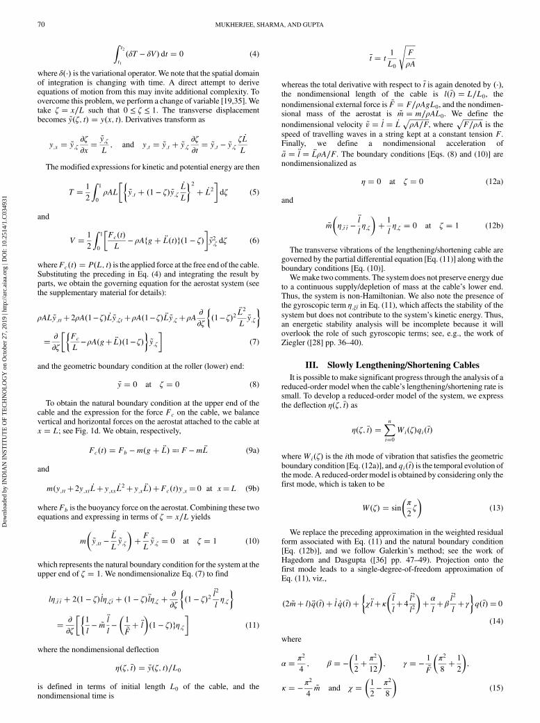
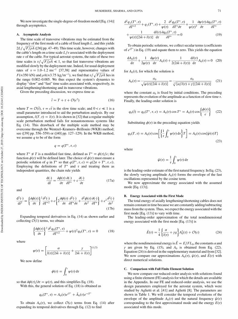
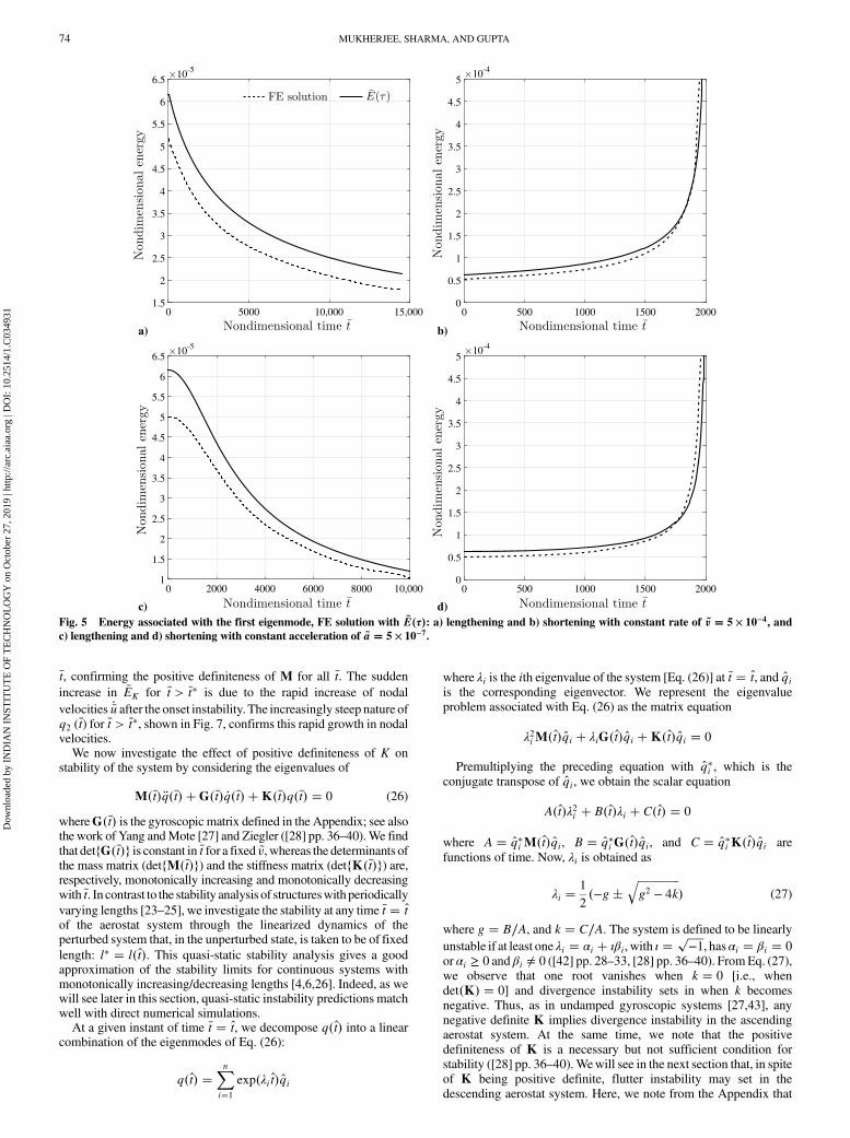
[Eq. (13)]; cf. Fig. 4.We present the evolution of energy associated with the first

eigenmode obtained from FE computations for various lengthening/

shortening rates in Fig. 5. Initially, the cable is deformed into theshape of the first eigenmode of a cablewith a constant length of l � 1,which is the initial length of the lengthening/shortening cable. The

initial configuration of the cable is shownwith a dashed line in Fig. 4.We also show the evolution of energy E�τ� obtained from theasymptotic analysis in the same figure. Our approximation for energyE�τ� again matches qualitatively with the energy associated with thefirst eigenmode of Eq. (A5). The departure from an exact match maybe explained as in the case of natural frequency.We see in Fig. 5 that the total energy of oscillations decreases for a

lengthening cable and grows to infinity as the length tends to zero fora shortening cable. A stability analysis of axially lengthening andshortening cables, based on the evolution of total energy in time, waspresented by Zhu and Ni [18]. These authors assume that the systemis unstable if the total energy associated with the perturbed cableincreases with time. Thus, axially shortening cables are claimed to beinherently unstable. However, there is no obvious reason for anenergetic stability criterion to indicate Lyapunov stability in thecurrent non-Hamiltonian system that has gyroscopic terms; see, e.g.,the works of Yang and Mote [27] and Ziegler ([28] pp. 36–40).Therefore, in the next section, we will investigate stability through aspectral analysis.

IV. Instability in Ascending Aerostats

In the previous section, we discussed the dynamics of a heavycable, for which its rate of lengthening/shortening is slow. We nowconsider the dynamics of the aerostat system for faster rates of ascent.Our FE computations, using parameters given in Table 1, show that,at a constant rate of ascent ~v � 0.0175, displacements of the lower

nodes start increasing rapidly after �t > 9.7 × 105; see Figs. 6a and 6b.

Additionally, for �t > ×105, the nodal displacements no longer remainoscillatory. Figures 6c and 6d show that, as time elapses, the upper

Table 1 Designparameters for the aerostat system

Parameter Value

Tether mass per unit length ρA 3.750 kg∕m−1

Aerostat mass� payload m 15,000 kgBuoyancy force Fb 500 kNAerostat radius r 30 m

a) b)

c) d)

,

,

,

Fig. 2 Time series response, FE solution withA0�τ�: a) lengthening and b) shortening cable with constant rate of ~v � 5 × 10−4, and c) lengthening and

d) shortening cable with constant acceleration of ~a � 5 × 10−7.

72 MUKHERJEE, SHARMA, AND GUPTA

Dow

nloa

ded

by I

ND

IAN

IN

STIT

UT

E O

F T

EC

HN

OL

OG

Y o

n O

ctob

er 2

7, 2

019

| http

://ar

c.ai

aa.o

rg |

DO

I: 1

0.25

14/1

.C03

4931

nodes gradually begin rapid and aperiodic motion. We willsubsequently identify this rapid increase of nodal deflections asinstability of ascending cables. Note that the jaggedness at the bottomof the cable is random, and it increases with the number of finiteelements. This is because the poststability behavior of the cablecannot be captured by the model, and thus the individual nodaldisplacements randomly approach infinity as the instability sets in.Figure 6 shows that instability first sets in at the lowest free

computational node (node 2) of the cable and then propagates

upward. Thus, we plot the deflection q2��t� of node 2 against �t toinvestigate how the ascending rate ~v affects the critical time �t � �t�;after which, the cable becomes unstable.The variation of q2 with �t for different constant rates ~v is shown in

Fig. 7.We see that, after a certain �t � �t�, q2 ceases to oscillate about amean. Instead, q2 increases rapidly for �t ≥ �t�, thereby destabilizing

the system. Figure 7 also shows that �t� reduces with increasing �v.Additionally, we observe that, at the onset of instability, the total

energy associated with the aerostat system �E becomes negative and

rapidly approaches −∞ as �t > �t�; see insets in Fig. 7. To understandwhy �E → −∞ for �t > �t�, we write the total energy as

�E � 1

2_qTM _q� 1

2qTKq (25)

where M and K are the global mass and stiffness matrices,respectively; and q and _q are the nodal displacement and velocitycolumn vectors, respectively. See the Appendix for details. The first

term in the preceding equation represents the kinetic energy �EK,

whereas the second term is the potential energy �EP of the system.

Now, for �E to be negative, either �EK, �EP, or both must be negative.From the Appendix, we find thatM is a diagonal matrix consisting ofstrictly nonnegative and real elements. Thus, M is positive definite

for all �t and �EK cannot be negative for any _q. Thus, it must be that �EP

becomes negative for �t ≥ �t�, which in turn implies thatK no longerremains positive definite after �t ≥ �t�.These observations are now validated by FE computations in

Fig. 8, which reports the variations of �E, �EK , and �EP with �t. Figure 8shows that �EP becomes negative before �E does, and it eventually

forces �E to become negative.We note that �EK remains positive for all

,,

,

c) d)

b)a)

Fig. 3 Evolution of the first natural frequency, FE solution with �ψ�τ�: a) lengthening and b) shortening cable with constant rate of ~v � 5 × 10−4, andc) lengthening and d) shortening cable with a constant acceleration of ~a � 5 × 10−7.

Fig. 4 Comparison of the shape of the first eigenmode of a cable in theζ � x∕L domain obtained from FE computations (dashed line) with the

single-mode approximation [Eq. (13)] (solid line).

MUKHERJEE, SHARMA, AND GUPTA 73

Dow

nloa

ded

by I

ND

IAN

IN

STIT

UT

E O

F T

EC

HN

OL

OG

Y o

n O

ctob

er 2

7, 2

019

| http

://ar

c.ai

aa.o

rg |

DO

I: 1

0.25

14/1

.C03

4931

�t, confirming the positive definiteness of M for all �t. The sudden

increase in �EK for �t > �t� is due to the rapid increase of nodal

velocities _�u after the onset instability. The increasingly steep nature ofq2 (�t) for �t > �t�, shown in Fig. 7, confirms this rapid growth in nodalvelocities.We now investigate the effect of positive definiteness of K on

stability of the system by considering the eigenvalues of

M��t� �q��t� �G��t� _q��t� �K��t�q��t� � 0 (26)

whereG��t� is the gyroscopic matrix defined in the Appendix; see alsothework of Yang andMote [27] and Ziegler ([28] pp. 36–40).We findthatdetfG��t�g is constant in �t for a fixed ~v, whereas the determinants ofthe mass matrix (detfM��t�g) and the stiffness matrix (detfK��t�g) are,respectively, monotonically increasing and monotonically decreasingwith �t. In contrast to the stability analysis of structureswithperiodicallyvarying lengths [23–25], we investigate the stability at any time �t � t̂of the aerostat system through the linearized dynamics of theperturbed system that, in the unperturbed state, is taken to be of fixed

length: l� � l�t̂�. This quasi-static stability analysis gives a goodapproximation of the stability limits for continuous systems withmonotonically increasing/decreasing lengths [4,6,26]. Indeed, as wewill see later in this section, quasi-static instability predictions matchwell with direct numerical simulations.At a given instant of time �t � t̂, we decompose q�t̂� into a linear

combination of the eigenmodes of Eq. (26):

q�t̂� �Xni�1

exp�λi t̂�q̂i

where λi is the ith eigenvalue of the system [Eq. (26)] at �t � t̂, and q̂iis the corresponding eigenvector. We represent the eigenvalueproblem associated with Eq. (26) as the matrix equation

λ2iM�t̂�q̂i � λiG�t̂�q̂i �K�t̂�q̂i � 0

Premultiplying the preceding equation with q̂�i , which is the

conjugate transpose of q̂i, we obtain the scalar equation

A�t̂�λ2i � B�t̂�λi � C�t̂� � 0

where A � q̂�i M�t̂�q̂i, B � q̂�i G�t̂�q̂i, and C � q̂�i K�t̂�q̂i are

functions of time. Now, λi is obtained as

λi �1

2�−g

����������������g2 − 4k

q� (27)

where g � B∕A, and k � C∕A. The system is defined to be linearly

unstable if at least one λi � αi � ιβi, with ι �������−1

p, hasαi � βi � 0

or αi ≥ 0 and βi ≠ 0 ([42] pp. 28–33, [28] pp. 36–40). FromEq. (27),we observe that one root vanishes when k � 0 [i.e., whendet�K� � 0] and divergence instability sets in when k becomesnegative. Thus, as in undamped gyroscopic systems [27,43], anynegative definite K implies divergence instability in the ascendingaerostat system. At the same time, we note that the positivedefiniteness of K is a necessary but not sufficient condition forstability ([28] pp. 36–40).Wewill see in the next section that, in spiteof K being positive definite, flutter instability may set in thedescending aerostat system. Here, we note from the Appendix that

,

, ,

a) b)

c) d)Fig. 5 Energy associated with the first eigenmode, FE solution with �E�τ�: a) lengthening and b) shortening with constant rate of ~v � 5 × 10−4, andc) lengthening and d) shortening with constant acceleration of ~a � 5 × 10−7.

74 MUKHERJEE, SHARMA, AND GUPTA

Dow

nloa

ded

by I

ND

IAN

IN

STIT

UT

E O

F T

EC

HN

OL

OG

Y o

n O

ctob

er 2

7, 2

019

| http

://ar

c.ai

aa.o

rg |

DO

I: 1

0.25

14/1

.C03

4931

det�G� < 0, which results in g < 0 for a descending aerostat system.

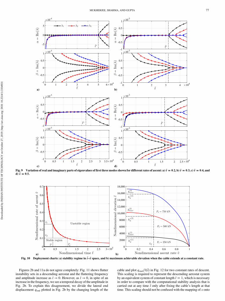
We now compare our remarks for λi with computations.We plot the evolution of the first three eigenvalues of Eq. (26) with

�t for different but constant rates of ascent in Fig. 9. Here, we observethat divergence instability sets in when λ1 � 0 at �t � �t�, which is

defined in Fig. 7. Thus, the critical time �t � �t� found in Fig. 7 indeeddefines the stability boundary for ascending aerostat systems for a

given ~v. Hence, the motion, observed in Figs. 6a–6d, is due to

divergence instability, which is now explained by employing a linear

stability analysis.The preceding analysis motivates us to develop deployment charts

for ascending aerostats. Figure 10a shows stable and unstable

operational regimes. This boundary separating two regimes is

obtained by noting the time t� at which the cable ascending at �vt firstbecomes unstable. Conversely, �vt is the minimum rate of ascent at

which instability will initiate at t�. Similarly, at a particular rate of

ascent (say, ~vd) we may find the critical time �t�d beyond which the

ascending aerostat is unstable.Figure 10b shows another deployment chart for the critical

elevation h�d that may be achieved in a stable manner at a given

constant rate of ascent ~vd. Figure 10b shows that, to achieve

maximum elevation, the deployment of the aerostat should be done

quasi statically, i.e., with j ~vdj ≪ 1. However, this is not practical.A possible alternative is to select a finite ~vd and augment the

buoyancy force Fb instead. As shown in Fig. 10b, the maximum

allowable elevation of the aerostat is greater at higher values of the net

upward pull F � Fb −mg; cf. Eq. (9a). The latter may be achieved

by expanding thevolumeof the aerostat. If the rate of deployment and

the desired elevation is given, we may select an optimal F from

Fig. 10b. We note from Fig. 10b that the overall maximum elevationachievable hmax is seenwhen the ascent rate is vanishingly small. Theelevation hmax is regulated by the length of the cable at which thetension P�0; t� at the bottom of the cable first becomes zero and,consequently, the aerostat system becomes unstable. At this time, theupward buoyancy force Fb balances the combined weight of theaerostat and the cable. This may be understood by noting that, whenP�0; t� vanishes, the resulting stiffness of the cable becomes zerolocally, and hence K becomes singular. We emphasize that, atnonzero rates of deployment, that vanishing of the base tension is notthe cause for the instability that regulates the maximum achievableelevation.Finally, the rate of deployment of aerostats may not be kept

constant during deployment. In Sec. VI, we investigate the case ofnonconstant deployment rates.

V. Instability in Descending Aerostats

It was shown in Figs. 3b, 3d, 4b, and 4d that the first naturalfrequency of the oscillation and total energy of a descending aerostatsystem approach infinity as the cable’s length l → 0. We nowinvestigate the stability of the aerostat system as it descends at aconstant rate by considering the evolution of the eigenvaluesof Eq. (26).Consider first the structure of thematricesM,G, andK in Eq. (26),

which is given in the Appendix. We observe that, for _l < 0,gyroscopic matrix G no longer remains positive definite. Thus, gbecomes negative in Eq. (27), resulting in a positive real part in theeigenvalues λi, i.e., the λi always have a αi > 0 with βi ≠ 0. This,

c) t = 10.5 × 105 d) t = 11.0 × 105

a) t = 8 × 105 b) t = 9.9 × 105

Fig. 6 Deflected shapes of the cable at different time instants while ascending at a constant rate of ~v � 0.0175.

MUKHERJEE, SHARMA, AND GUPTA 75

Dow

nloa

ded

by I

ND

IAN

IN

STIT

UT

E O

F T

EC

HN

OL

OG

Y o

n O

ctob

er 2

7, 2

019

| http

://ar

c.ai

aa.o

rg |

DO

I: 1

0.25

14/1

.C03

4931

in turn, introduces flutter instability in the system [27]. Thisobservation is confirmed by the evolution in Fig. 11 of λ1, λ2, and λ3found from FE computations. Figure 11 shows that λi (i � 1; 2; 3)always have αi > 0 and βi ≠ 0. Themagnitude of αi initially remains

very small. However, as l → 0, α2 and α3 grow to infinity. This is

because det�M� → 0 as l → 0 so thatM eventually becomes singular

at l � 0. Interestingly, α1 0 for all l�t� because of the presence of aheavy, lumped mass (the aerostat) at the end of the cable, which

causes α1 ≪ α2; α3; see the supplementary material for details.

Figures 11a and 11b also show that the βi increase with lowering land, eventually, grow to infinity as l → 0 and M becomes singular.The increase in βi is in agreement with the asymptotic analysis ofFig. 2b, in which we se high-frequency oscillations as l → 0.Physically, we may interpret a cable of l ≪ 1 as a system with veryhigh stiffness; indeed, we note from the Appendix that every elementofK ∝ 1∕l. Thus, analogous to a single-degree-of-freedom system,the aerostat system with high stiffness will have large natural

frequencies, which are proportional to the eigenvalues of��������������M−1K

p.

a) b)

c) d)Fig. 7 Evolutions of deflection of node 2 and total nondimensional energy �E (inset) in time for different rates of ascent: a) ~v � 0.2, b) ~v � 0.3, c) ~v � 0.4,and d) ~v � 0.5.

a) b)Fig. 8 Evolutions of total nondimensional energy �E, kinetic energy �EK and potential energy �EP with time for different rates of ascending: a) ~v � 0.2 andb) ~v � 0.3.

76 MUKHERJEE, SHARMA, AND GUPTA

Dow

nloa

ded

by I

ND

IAN

IN

STIT

UT

E O

F T

EC

HN

OL

OG

Y o

n O

ctob

er 2

7, 2

019

| http

://ar

c.ai

aa.o

rg |

DO

I: 1

0.25

14/1

.C03

4931

Figures 2b and 11a do not agree completely: Fig. 11 shows flutterinstability sets in a descending aerostat and the fluttering frequency

and amplitude increase as l → 0. However, as l → 0, in spite of an

increase in the frequency, we see a temporal decay of the amplitude inFig. 2b. To explain this disagreement, we divide the lateral end

displacement qend plotted in Fig. 2b by the changing length of the

cable and plot qend∕l��t� in Fig. 12 for two constant rates of descent.This scaling is required to represent the descending aerostat system

by an equivalent system of constant length l � 1, which is necessaryin order to compare with the computational stability analysis that iscarried out at any time �t only after fixing the cable’s length at that

time. This scaling should not be confused with the mapping of x onto

,

,

,

,

,

a) b)Fig. 10 Deployment charts: a) stability regime in �t– ~v space, and b) maximum achievable elevation when the cable extends at a constant rate.

a) b)

c) d)Fig. 9 Variation of real and imaginary parts of eigenvalues of first threemodes shown for different rates of ascent: a) ~v � 0.2, b) ~v � 0.3, c) ~v � 0.4, andd) ~v � 0.5.

MUKHERJEE, SHARMA, AND GUPTA 77

Dow

nloa

ded

by I

ND

IAN

IN

STIT

UT

E O

F T

EC

HN

OL

OG

Y o

n O

ctob

er 2

7, 2

019

| http

://ar

c.ai

aa.o

rg |

DO

I: 1

0.25

14/1

.C03

4931

ζ in Sec. II, which was introduced to map the aerostat system withchanging lengths onto a unit length. The lateral displacement y�x; t�,however, was scaled by the initial length L0 in Sec. II. Once we scaleq2 of Fig. 2b by l��t�, we do observe a flutter instability in thedescending aerostat in Fig. 12, which confirms the predictions inFig. 11, which were made on the basis of the system’s eigenvalues.Finally, increasing flutter as l → 0 is similar to what is observed in

shortening pendulums [44–46], in which the amplitude of oscillationsblows up as l → 0, and consequently the small amplitude assumptionceases to hold. Instability in shortening cables was explained on thebasis of the temporal evolution of total energy by Zhu and Ni [18]. Incontrast, we have followed a spectral analysis ([42] pp. 28–33) that, asdiscussed at the end of Sec. II, is the correct way to investigateinstability in non-Hamiltonian gyroscopic systems (Yang and Mote[27] and Ziegler [28] pp. 36–40). From a practical standpoint, to avoidfluttering, the tether of the aerostat must have a finite length evenwhenit is retracted to its lowest position. Moreover, retraction must be donewith intermediate breaks; during which, the perturbations of the cablecan be damped out by viscous air drag.We now move on to investigate the effect of air flow on the

dynamics of the cable.

VI. Forced Vibration

So far, we have not incorporated external forces (e.g., from airdrag) into our analysis.We now investigate the forced response of thesystem. We begin by introducing a model for aerodynamic forces.

A. Aerodynamic Forces

Consider a lengthening/shortening cable that is attached to an

aerostat, which is modeled as a rigid sphere. For simplicity, we

consider air drag only on the aerostat and not on the cable. This is

acceptable as a first approximation because we expect the drag on the

cable to be much smaller as compared to that on the aerostat. A model

for the dynamics of a rigid sphere (aerostat) submerged completely in a

Newtonian fluid (air) is as follows [29–31]:

mdVi

dt� mf

�DuiDt

− νΔui�Y�t�

−1

2mf

d

dt�Vi�t� − ui�Y�t�; t��

− 6πrμ�Vi�t� − ui�Y�t�; t�� � �m −mf�gi � F�e�i (28)

where the operator D�⋅�∕Dt is defined as

D�⋅�iDt

� ∂�⋅�i∂t

� ∂�⋅�i∂xj

�⋅�j

and the subscripts i and j represent different components of a vector;Δis the Laplacian operator; mf is the mass of air displaced by the

aerostat; ν and μ are kinematic and dynamic viscosities of air,

respectively; r is the radius of the aerostat with its center located at aposition Y�t� and moving at a velocity V; and u is the velocity of air.

The termmf�Dui∕Dt − νΔui� on the right-hand side of Eq. (28) is dueto the pressure gradient imposed by the air flow. The second term

,

a) b)Fig. 12 Temporal evolution of the perturbedmotion of the aerostat relative to its changing length for two constant descending rates: a) ~v � −0.0001 andb) ~v � −0.001.

,

a) b)Fig. 11 Variation of real and imaginary parts of the eigenvalues of the first three modes, shown for two different rates of descent: a) ~v � −0.0001 andb) ~v � −0.001.

78 MUKHERJEE, SHARMA, AND GUPTA

Dow

nloa

ded

by I

ND

IAN

IN

STIT

UT

E O

F T

EC

HN

OL

OG

Y o

n O

ctob

er 2

7, 2

019

| http

://ar

c.ai

aa.o

rg |

DO

I: 1

0.25

14/1

.C03

4931

0.5mfd�Vi�t� − ui�Y�t�; t��∕dt

is the added mass on the aerostat. The next three terms represent,

respectively, the viscous Stokes drag, buoyancy, and (nonaerody-

namic) external force F�e� due to, in our case, the cable.We consider only horizontal air flow for which the speedmay vary

vertically and with time. As μair is about 10−5 kg∕�m−1 ⋅ s−1�, we

take air to be inviscid. Because aerodynamic forces act only on the

aerostat, the only change in the equations of motion will be in the

boundary condition at ζ � 1 [i.e., Eq. (10)] that, after non-dimensionalizing (as in Sec. II), becomes

~m

�η;�t �t � 2

_l

l�1 − ζ�η;ζ�t �

_l2

l2�1 − ζ�2η;ζζ − ζ

�l

lη;ζ

�

� 1

lη;ζ � ~mf

�~u;�t �

~u

l~u;ζ

�−1

2~mf

�η;�t �t

� 2_l

l�1 − ζ�η;ζ�t �

_l2

l2f�1� ζ2�η;ζg;ζ � �1 − ζ�

�l

lη;ζ − ~u;�t

�(29)

a) b)Fig. 13 Representations of a) steadyvelocity profile of air, andb) end-tip displacement of cable. The aerostat is ascending at a constant rate of ~v � 0.0025.

a) b)

c) d)

Fig. 14 Representations of a) variation of first three natural frequencies of the system with time, b) the time series response of end-tip displacement,c) variation of total energy, d) frequency domain response of the system.

MUKHERJEE, SHARMA, AND GUPTA 79

Dow

nloa

ded

by I

ND

IAN

IN

STIT

UT

E O

F T

EC

HN

OL

OG

Y o

n O

ctob

er 2

7, 2

019

| http

://ar

c.ai

aa.o

rg |

DO

I: 1

0.25

14/1

.C03

4931

where ~u is the nondimensional velocity of air: ~u � u������������ρA∕F

p, and

~mf � mf∕L0ρA is the nondimensional mass of the air displaced by

the aerostat. In the preceding equation, we identified V and Y�t� inEq. (28) with, respectively, ~y;tt and ζ � 1. We now investigate the

effect of aerodynamic forces on the aerostat. Note that we ignore

changes in the tension in the cable due to its lateral deflection. This is

because of the very small inclination of the cable with the vertical

(≈1.5 deg) as obtained from computations with practical aerostat

data under wind load; see Fig. 13. The computation scheme is as

discussed in the Appendix, but it now includes the modified

boundary condition [Eq. (29)].

B. Results

In this section,we assume the density of air (ρair � 1.205 kg∕m−3)

remains constant with the altitude. We first consider a steady air flow

profile, shown in Fig. 13a. The flow profile is obtained from the air

flow data provided by Badesha and Bunn [47]. This air flow exerts

drag on the aerostat. The temporal response for an ascending aerostat

with a constant of ~v � 0.0025 is shown in Fig. 13b. The response issimilar to that observed during free vibration, except that the mean of

the oscillation shifts in the direction of air flow.

We now consider an air flow that is uniform in space but for which

the amplitude changes with time as ~u��t� � 0.1 sin� ~ωf �t�. The cableextends at a constant rate of ~v � 0.0025. As the aerostat ascends, thenatural frequencies of the system decrease. The temporal variations

of the first three natural frequencies ~ω1, ~ω2, and ~ω3 of the system are

depicted in Fig. 14a.We note from Fig. 14a that therewill always be a

time �t� after which one of the natural frequencies of the system will

match ~ωf. As an example, we take ~ωf � 0.0075 and note the

corresponding �t� from Fig. 14a at which ~ωf equals ~ω1. As shown in

Fig. 14b, the system resonates when �t � �t�. Figure 14c confirms thatthere is a sudden change in the total energy of the system at �t � �t�.However, the aerostat’s displacement qend cannot grow continuouslybecause the natural frequency of the system shifts away from ~ωf

when time goes beyond �t�. Finally, the frequency domain response ofthe system is shown in Fig. 14d. The surface shown in Fig. 14d is theenvelope of qend for various excitation frequencies ~ωf. We note that

large-amplitude vibrations occur in the range of 0 < ~ωf < 0.03. Our

computations predict that, when ~ωf ≥ 0.03, vibration amplitudes are

not very large because they are driven by resonant interactions withthe second or higher modes of the system. Figure 14d matchesqualitatively with the experimental results of Yamamoto et al. [48],who investigated forced vibration of a lengthening/shortening cablethat was fixed at its ends.Next, we investigate the frequency domain response of a

descending aerostat. The aerostat system is taken to be retracting at aconstant rate of ~v � 0.0025. We note from Fig. 15a that the firstnatural frequency slowly grows from ~ω1 � 0.08. Therefore, weexpect resonance when ~ωf ≥ 0.08. We again define time �t� in

Fig. 15a as the time at which ~ω1 � ~ωf. We set ~ωf � 0.1 and obtain

the time domain response for end deflection and velocity; seeFig. 15b.We observe from Fig. 15b that the amplitude begins to growat �t � �t�. As before, the amplitude cannot grow continuously as thefirst natural frequency of the system shifts from ~ωf. The total energy

of a shortening cable is seen to increase with time for reasonsdiscussed in Sec. III. We find from Fig. 15c that energy now growseven more rapidly due to resonance. Finally, the frequency domainresponse of the system is depicted in Fig. 15d. We note thatamplitudes do not grow for excitation frequencies beyond 0.3. Itsuggests that resonance in a shortening cable is significant only for~ωf near its first natural frequency ~ω1. Figure 15d is also in a good

c) d)

a) b)

Fig. 15 Representations of a) variation of first three natural frequencies of the system in time, b) time series response of end-tip displacement, c) variationof total energy, and d) frequency domain response of the system.

80 MUKHERJEE, SHARMA, AND GUPTA

Dow

nloa

ded

by I

ND

IAN

IN

STIT

UT

E O

F T

EC

HN

OL

OG

Y o

n O

ctob

er 2

7, 2

019

| http

://ar

c.ai

aa.o

rg |

DO

I: 1

0.25

14/1

.C03

4931

qualitative match with the experimentally obtained frequencydomain response of a shortening cable that has both of its endsfixed [48].We end this section with two comments. The waviness in the

energy plots of Figs. 14c and 15c is due to the periodicity in theaerodynamic forcing. Thewaviness in the surface plots Figs. 14d and15d is due to the waviness in the envelope of the amplitudes, asextracted directly from the simulations. Waviness in the frequencydomain response was also observed in the experiments on forcedvibrations of lengthening/shortening cables by Yamamoto et al. [48].

VII. Case Studies

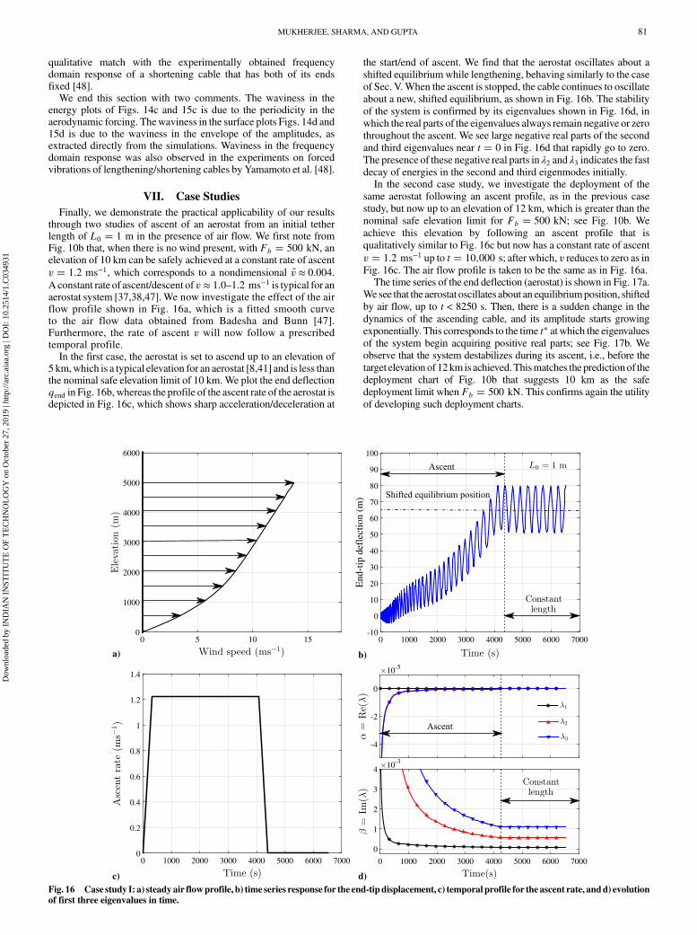
Finally, we demonstrate the practical applicability of our resultsthrough two studies of ascent of an aerostat from an initial tetherlength of L0 � 1 m in the presence of air flow. We first note fromFig. 10b that, when there is no wind present, with Fb � 500 kN, anelevation of 10 km can be safely achieved at a constant rate of ascent

v � 1.2 ms−1, which corresponds to a nondimensional ~v ≈ 0.004.

A constant rate of ascent/descent of v ≈ 1.0–1.2 ms−1 is typical for anaerostat system [37,38,47].We now investigate the effect of the airflow profile shown in Fig. 16a, which is a fitted smooth curveto the air flow data obtained from Badesha and Bunn [47].Furthermore, the rate of ascent v will now follow a prescribedtemporal profile.In the first case, the aerostat is set to ascend up to an elevation of

5 km,which is a typical elevation for an aerostat [8,41] and is less thanthe nominal safe elevation limit of 10 km. We plot the end deflectionqend in Fig. 16b,whereas the profile of the ascent rate of the aerostat isdepicted in Fig. 16c, which shows sharp acceleration/deceleration at

the start/end of ascent. We find that the aerostat oscillates about a

shifted equilibrium while lengthening, behaving similarly to the case

of Sec. V.When the ascent is stopped, the cable continues to oscillate

about a new, shifted equilibrium, as shown in Fig. 16b. The stability

of the system is confirmed by its eigenvalues shown in Fig. 16d, in

which the real parts of the eigenvalues always remain negative or zero

throughout the ascent. We see large negative real parts of the second

and third eigenvalues near t � 0 in Fig. 16d that rapidly go to zero.

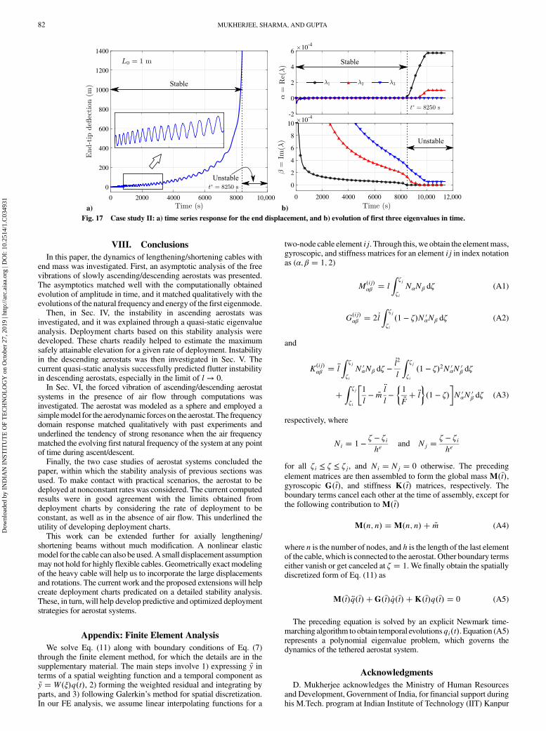
The presence of these negative real parts in λ2 and λ3 indicates the fastdecay of energies in the second and third eigenmodes initially.In the second case study, we investigate the deployment of the

same aerostat following an ascent profile, as in the previous case

study, but now up to an elevation of 12 km, which is greater than the

nominal safe elevation limit for Fb � 500 kN; see Fig. 10b. We

achieve this elevation by following an ascent profile that is

qualitatively similar to Fig. 16c but now has a constant rate of ascent

v � 1.2 ms−1 up to t � 10;000 s; after which, v reduces to zero as inFig. 16c. The air flow profile is taken to be the same as in Fig. 16a.The time series of the end deflection (aerostat) is shown in Fig. 17a.

We see that the aerostat oscillates about an equilibriumposition, shifted

by air flow, up to t < 8250 s. Then, there is a sudden change in the

dynamics of the ascending cable, and its amplitude starts growing

exponentially. This corresponds to the time t� atwhich the eigenvaluesof the system begin acquiring positive real parts; see Fig. 17b. We

observe that the system destabilizes during its ascent, i.e., before the

target elevation of 12km is achieved.Thismatches the predictionof the

deployment chart of Fig. 10b that suggests 10 km as the safe

deployment limit when Fb � 500 kN. This confirms again the utility

of developing such deployment charts.

a) b)

c) d)Fig. 16 Case study I: a) steady air flowprofile, b) time series response for the end-tip displacement, c) temporal profile for the ascent rate, andd) evolutionof first three eigenvalues in time.

MUKHERJEE, SHARMA, AND GUPTA 81

Dow

nloa

ded

by I

ND

IAN

IN

STIT

UT

E O

F T

EC

HN

OL

OG

Y o

n O

ctob

er 2

7, 2

019

| http

://ar

c.ai

aa.o

rg |

DO

I: 1

0.25

14/1

.C03

4931

VIII. Conclusions

In this paper, the dynamics of lengthening/shortening cables withend mass was investigated. First, an asymptotic analysis of the freevibrations of slowly ascending/descending aerostats was presented.The asymptotics matched well with the computationally obtainedevolution of amplitude in time, and it matched qualitatively with theevolutions of the natural frequency and energy of the first eigenmode.Then, in Sec. IV, the instability in ascending aerostats was

investigated, and it was explained through a quasi-static eigenvalueanalysis. Deployment charts based on this stability analysis weredeveloped. These charts readily helped to estimate the maximumsafely attainable elevation for a given rate of deployment. Instabilityin the descending aerostats was then investigated in Sec. V. Thecurrent quasi-static analysis successfully predicted flutter instabilityin descending aerostats, especially in the limit of l → 0.In Sec. VI, the forced vibration of ascending/descending aerostat

systems in the presence of air flow through computations wasinvestigated. The aerostat was modeled as a sphere and employed asimplemodel for the aerodynamic forces on the aerostat.The frequencydomain response matched qualitatively with past experiments andunderlined the tendency of strong resonance when the air frequencymatched the evolving first natural frequency of the system at any pointof time during ascent/descent.Finally, the two case studies of aerostat systems concluded the

paper, within which the stability analysis of previous sections wasused. To make contact with practical scenarios, the aerostat to bedeployed at nonconstant rates was considered. The current computedresults were in good agreement with the limits obtained fromdeployment charts by considering the rate of deployment to beconstant, as well as in the absence of air flow. This underlined theutility of developing deployment charts.This work can be extended further for axially lengthening/

shortening beams without much modification. A nonlinear elasticmodel for the cable can also be used.A small displacement assumptionmay not hold for highly flexible cables. Geometrically exact modelingof the heavy cable will help us to incorporate the large displacementsand rotations. The current work and the proposed extensions will helpcreate deployment charts predicated on a detailed stability analysis.These, in turn, will help develop predictive and optimized deploymentstrategies for aerostat systems.

Appendix: Finite Element Analysis

We solve Eq. (11) along with boundary conditions of Eq. (7)through the finite element method, for which the details are in thesupplementary material. The main steps involve 1) expressing ~y interms of a spatial weighting function and a temporal component as~y � W�ξ�q�t�, 2) forming the weighted residual and integrating byparts, and 3) following Galerkin’s method for spatial discretization.In our FE analysis, we assume linear interpolating functions for a

two-node cable element ij. Through this,we obtain the elementmass,gyroscopic, and stiffness matrices for an element ij in index notationas (α; β � 1; 2)

M�ij�αβ � l

Zζj

ζi

NαNβ dζ (A1)

G�ij�αβ � 2_l

Zζj

ζi

�1 − ζ�N 0αNβ dζ (A2)

and

K�ij�αβ � �l

Zζj

ζi

N 0αNβ dζ −

_l2

l

Zζj

ζi

�1 − ζ�2N 0αN

0β dζ

�Z

ζj

ζi

�1

l− ~m

�l

l−�1

~F� �l

��1 − ζ�

�N 0

αN0β dζ (A3)

respectively, where

Ni � 1 −ζ − ζihe

and Nj �ζ − ζihe

for all ζi ≤ ζ ≤ ζj, and Ni � Nj � 0 otherwise. The preceding

element matrices are then assembled to form the global mass M��t�,gyroscopic G��t�, and stiffness K��t� matrices, respectively. Theboundary terms cancel each other at the time of assembly, except forthe following contribution to M��t�

M�n; n� � M�n; n� � ~m (A4)

where n is the number of nodes, and h is the length of the last elementof the cable, which is connected to the aerostat. Other boundary termseither vanish or get canceled at ζ � 1. We finally obtain the spatiallydiscretized form of Eq. (11) as

M��t� �q��t� �G��t� _q��t� �K��t�q��t� � 0 (A5)

The preceding equation is solved by an explicit Newmark time-marching algorithm toobtain temporal evolutionsqi�t�. Equation (A5)represents a polynomial eigenvalue problem, which governs thedynamics of the tethered aerostat system.

Acknowledgments

D. Mukherjee acknowledges the Ministry of Human Resourcesand Development, Government of India, for financial support duringhis M.Tech. program at Indian Institute of Technology (IIT) Kanpur

a) b)Fig. 17 Case study II: a) time series response for the end displacement, and b) evolution of first three eigenvalues in time.

82 MUKHERJEE, SHARMA, AND GUPTA

Dow

nloa

ded

by I

ND

IAN

IN

STIT

UT

E O

F T

EC

HN

OL

OG

Y o

n O

ctob

er 2

7, 2

019

| http

://ar

c.ai

aa.o

rg |

DO

I: 1

0.25

14/1

.C03

4931

when this research was conducted. We are grateful to C. Venkatesanof Aerospace Engineering, IIT Kanpur, for encouraging us to take upthis research and for insightful evaluations. We would like to thankAbhinav Dehadrai of Mechanical Engineering, IIT Kanpur, forhelpful discussions. Finally, we would like to thank an anonymousreferee for critical comments that greatly improved this work.

References

[1] Carrier, G. F., “The Spaghetti Problem,” American Mathematical

Monthly, Vol. 56, No. 10, 1949, pp. 669–672.doi:10.2307/2305560

[2] Mansfield, L., and Simmonds, J. G., “The Reverse Spaghetti Problem:Drooping Motion of an Elastica Issuing from a Horizontal Guide,”Journal of Applied Mechanics, Vol. 54, No. 1, 1987, pp. 147–150.doi:10.1115/1.3172949

[3] Stylianou,M., and Tabarrok, B., “Finite Element Analysis of an AxiallyMoving Beam, Part I: Time Integration,” Journal of Sound and

Vibration, Vol. 178, No. 4, 1994, pp. 433–453.doi:10.1006/jsvi.1994.1497

[4] Stylianou,M., and Tabarrok, B., “Finite Element Analysis of an AxiallyMoving Beam, Part II: Stability Analysis,” Journal of Sound and

Vibration, Vol. 178, No. 4, 1994, pp. 455–481.doi:10.1006/jsvi.1994.1498

[5] Terumichi,Y.,Ohtsuka,M.,Yoshizawa,M., Fukawa,Y., andTsujioka,Y.,“Nonstationary Vibrations of a String with Time-Varying Length and aMass-Spring Attached at the Lower End,” Nonlinear Dynamics, Vol. 12,No. 1, 1997, pp. 39–55.doi:10.1023/A:1008224224462

[6] Gosselin, F., Paidoussis, M., and Misra, A., “Stability of a Deploying/Extruding Beam in Dense Fluid,” Journal of Sound and Vibration,Vol. 299, No. 1, 2007, pp. 123–142.doi:10.1016/j.jsv.2006.06.050

[7] Kawaguti, K., Terumichi, Y., Takehara, S., Kaczmarczyk, S., andSogabe,K., “The Study of the TetherMotionwith Time-VaryingLengthUsing the Absolute Nodal Coordinate Formulation with MultipleNonlinear Time Scales,” Journal of System Design and Dynamics,Vol. 1, No. 3, 2007, pp. 491–500.doi:10.1299/jsdd.1.491

[8] Aglietti, G., “Dynamic Response of a High-Altitude Tethered BalloonSystem,” Journal of Aircraft, Vol. 46, No. 6, 2009, pp. 2032–2040.doi:10.2514/1.43332

[9] Jones, S., and Krausman, J., “Nonlinear Dynamic Simulation of aTetheredAerostat,” Journal of Aircraft, Vol. 19,No. 8, 1982, pp. 679–686.doi:10.2514/3.57449

[10] Lambert, C., andNahon,M., “StabilityAnalysis of aTetheredAerostat,”Journal of Aircraft, Vol. 40, No. 4, 2003, pp. 705–715.doi:10.2514/2.3149

[11] Kang, W., and Lee, I., “Analysis of Tethered Aerostat Response underAtmospheric Turbulence Considering Nonlinear Cable Dynamics,”Journal of Aircraft, Vol. 46, No. 1, 2009, pp. 343–348.doi:10.2514/1.38599

[12] Hembree, B., and Slegers, N., “Tethered Aerostat Modeling Using anEfficient Recursive Rigid-Body Dynamics Approach,” Journal of

Aircraft, Vol. 48, No. 2, 2011, pp. 623–632.doi:10.2514/1.C031179

[13] Mi, L., and Gottlieb, O., “Nonlinear Dynamics and Internal Resonancesof a Planar Multi-Tethered Spherical Aerostat in Modulated Flow,”Meccanica, Vol. 51, No. 11, 2016, pp. 2689–2712.doi:10.1007/s11012-016-0486-z

[14] Mankala, K. K., and Agrawal, S. K., “Dynamic Modeling andSimulation of Satellite Tethered Systems,” Journal of Vibration and

Acoustics, Vol. 127, No. 2, 2005, pp. 144–156.doi:10.1115/1.1891811

[15] Mankala, K. K., and Agrawal, S. K., “Dynamic Modeling of SatelliteTether Systems Using Newton’s Laws and Hamilton’s Principle,”Journal of Vibration and Acoustics, Vol. 130, No. 1, 2008, Paper014501.doi:10.1115/1.2776342

[16] Pesce, C. P., “The Application of Lagrange Equations to MechanicalSystems with Mass Explicitly Dependent on Position,” Journal of

Applied Mechanics, Vol. 70, No. 5, 2003, pp. 751–756.doi:10.1115/1.1601249

[17] Crellin, E. B., Janssens, F., Poelaert, D., Steiner,W., and Troger, H., “OnBalance and Variational Formulations of the Equation of Motion of aBody Deploying Along a Cable,” Journal of Applied Mechanics,Vol. 64, No. 2, 1997, pp. 369–374.doi:10.1115/1.2787316

[18] Zhu,W., and Ni, J., “Energetics and Stability of TranslatingMedia withan Arbitrarily Varying Length,” Journal of Vibration and Acoustics,

Vol. 122, No. 3, 2000, pp. 295–304.

doi:10.1115/1.1303003[19] Vu-Quoc, L., and Li, S., “Dynamics of Sliding Geometrically-Exact

Beams: Large Angle Maneuver and Parametric Resonance,” Computer

Methods in AppliedMechanics and Engineering, Vol. 120, No. 1, 1995,

pp. 65–118.

doi:10.1016/0045-7825(94)00051-N[20] Chung, J., Han, C., and Yi, K., “Vibration of an Axially Moving

String with Geometric Non-Linearity and Translating Acceleration,”

Journal of Sound and Vibration, Vol. 240, No. 4, 2001,

pp. 733–746.

doi:10.1006/jsvi.2000.3241[21] Parker, R., “Supercritical SpeedStability of the Trivial Equilibriumof an

Axially-MovingString on anElastic Foundation,” Journal of Sound and

Vibration, Vol. 221, No. 2, 1999, pp. 205–219.

doi:10.1006/jsvi.1998.1936[22] Wickert, J., and Mote, C., “Classical Vibration Analysis of Axially

Moving Continua,” Journal of AppliedMechanics, Vol. 57, No. 3, 1990,pp. 738–744.doi:10.1115/1.2897085

[23] Elmaraghy, R., and Tabarrok, B., “On the Dynamic Stability of anAxially Oscillating Beam,” Journal of the Franklin Institute, Vol. 300,No. 1, 1975, pp. 25–39.doi:10.1016/0016-0032(75)90185-4

[24] Zajaczkowski, J., and Lipiński, J., “Instability of the Motion of a Beamof Periodically Varying Length,” Journal of Sound and Vibration,Vol. 63, No. 1, 1979, pp. 9–18.doi:10.1016/0022-460X(79)90373-0

[25] Hyun, S., and Yoo, H., “Dynamic Modelling and Stability Analysis ofAxiallyOscillatingCantilever Beams,” Journal of Sound andVibration,Vol. 228, No. 3, 1999, pp. 543–558.doi:10.1006/jsvi.1999.2427

[26] Nawrotzki, P., and Eller, C., “Numerical Stability Analysis in StructuralDynamics,”ComputerMethods in AppliedMechanics andEngineering,Vol. 189, No. 3, 2000, pp. 915–929.doi:10.1016/S0045-7825(99)00407-7

[27] Yang, S.-M., and Mote, C., “Stability of Non-Conservative LinearDiscrete Gyroscopic Systems,” Journal of Sound and Vibration,Vol. 147, No. 3, 1991, pp. 453–464.doi:10.1016/0022-460X(91)90493-4

[28] Ziegler, H., Principles of Structural Stability, Vol. 35, BirkhäuserBoston, Cambridge, MA, 2013, pp. 36–40.doi:10.1007/978-3-0348-5912-7

[29] Tchen, C.-M., “Mean Value and Correlation Problems Connectedwith the Motion of Small Particles Suspended in a Turbulent Fluid,”Ph.D. Thesis, Delft Univ. of Technology, Delft, The Netherlands,1947.

[30] Corrsin, S., and Lumley, J., “On the Equation of Motion for a Particle inTurbulent Fluid,” Applied Scientific Research, Vol. 6, No. 2, 1956,

pp. 114–116.

doi:10.1007/BF03185030[31] Maxey, M. R., and Riley, J. J., “Equation of Motion for a Small Rigid

Sphere in a Nonuniform Flow,” Physics of Fluids, Vol. 26, No. 4, 1983,

pp. 883–889.

doi:10.1063/1.864230[32] Mukherjee, D., “Dynamics and Stability of Lengthening and Shortening

Heavy Cables with EndMass,”M.S. Thesis, Indian Inst. of Technology

Kanpur, India, 2016.[33] Miranker, W. L., “The Wave Equation in a Medium in Motion,”

IBM Journal of Research and Development, Vol. 4, No. 1, 1960,

pp. 36–42.

doi:10.1147/rd.41.0036[34] Renshaw, A. A., Rahn, C. D., Wickert, J. A., and Mote, C. D., “Energy

and Conserved Functionals for Axially Moving Materials,” Journal of

Vibration and Acoustics, Vol. 120, No. 2, 1998, p. 634.

doi:10.1115/1.2893875[35] Roy, A., and Chatterjee, A., “Vibrations of a Beam in Variable Contact

with a Flat Surface,” Journal of Vibration and Acoustics, Vol. 131,

No. 4, 2009, Paper 041010.

doi:10.1115/1.3086930[36] Hagedorn, P., and Dasgupta, A., Vibrations and Waves in Continuous

Mechanical Systems, Wiley, New York, 2007, pp. 47–49.[37] Reed, H., and Sechrist, J., “Tethered Aerostats—Technology Improve-

ments,” 2nd Lighter Than Air Systems Technology Conference, Lighter-

Than-Air Conferences, AIAA Paper 1977-1184, 1977.

doi:10.2514/6.1977-1184

MUKHERJEE, SHARMA, AND GUPTA 83

Dow

nloa

ded

by I

ND

IAN

IN

STIT

UT

E O

F T

EC

HN

OL

OG

Y o

n O

ctob

er 2

7, 2

019

| http

://ar

c.ai

aa.o

rg |

DO

I: 1

0.25

14/1

.C03

4931

[38] Badesha, S. S., Euler, A. J., and Schroeder, L., “Very High AltitudeTethered Balloon Trajectory Simulation,” AIAA Atmospheric Flight

Mechanics Conference, AIAA Paper 1996-3440, 1996.doi:10.2514/6.1996-3440

[39] Bender, C. M., and Orszag, S. A., Advanced Mathematical Methods for

Scientists and Engineers, Springer Science and Business Media,New York, 1978, pp. 556–559.doi:10.1007/978-1-4757-3069-2

[40] Hinch, E. J., Perturbation Methods, Cambridge Univ. Press, New York,1991, pp. 127–129.

[41] Aglietti, G., Markvart, T., Tatnall, A., and Walker, S., “Solar PowerGeneration Using High Altitude Platforms Feasibility and Viability,”Progress in Photovoltaics: Research and Applications, Vol. 16, No. 4,2008, pp. 349–359.doi:10.1002/pip.v16:4

[42] LaSalle, J. P., and Lefschetz, S., Stability by Liapunov’s Direct Method:

With Applications, Vol. 4, Academic Press, New York, 1961.[43] Huseyin, K., Hagedorn, P., and Teschner,W., “On the Stability of Linear

Conservative Gyroscopic Systems,” Zeitschrift für Angewandte

Mathematik und Physik, Vol. 34, No. 6, 1983, pp. 807–815.doi:10.1007/BF00949057

[44] Brearley, M. N., “The Simple Pendulum with Uniformly ChangingString Length,” Proceedings of the Edinburgh Mathematical Society,Vol. 15, No. 1, 1966, pp. 61–66.doi:10.1017/s0013091500013365

[45] Ross, D. K., “The Behaviour of a Simple Pendulum with UniformlyShortening String Length,” International Journal of Non-Linear

Mechanics, Vol. 14, No. 3, 1979, pp. 175–182.doi:10.1016/0020-7462(79)90034-9

[46] Asadi-Zeydabadi, M., “Bessel Function and Damped Simple HarmonicMotion,” Journal of Applied Mathematics and Physics, Vol. 2, No. 4,2014, pp. 26–34.doi:10.4236/jamp.2014.24004

[47] Badesha, S. S., and Bunn, J. C., “Dynamic Simulation of High AltitudeTethered Balloon System Subject to Thunderstorm Windfield,” AIAA

Atmospheric Flight Mechanics Conference, AIAA Paper 2002-4614,2002.doi:10.2514/6.2002-4614

[48] Yamamoto, T., Yasuda, K., and Kato, M., “Vibrations of a String withTime-Variable Length,” Bulletin of Japan Society of Mechanical

Engineers, Vol. 21, No. 162, 1978, pp. 1677–1684.doi:10.1299/jsme1958.21.1677

84 MUKHERJEE, SHARMA, AND GUPTA

Dow

nloa

ded

by I

ND

IAN

IN

STIT

UT

E O

F T

EC

HN

OL

OG

Y o

n O

ctob

er 2

7, 2

019

| http

://ar

c.ai

aa.o

rg |

DO

I: 1

0.25

14/1

.C03

4931