dynamics of nitrogen-fixing cyanobacteria with heterocysts

Marine and Freshwater Research 2020, 71, 644–658 © CSIRO 2020 https://doi.org/10.1071/MF18361

of 35

Supplementary material

Dynamics of nitrogen-fixing cyanobacteria with heterocysts: a stoichiometric model

James P. GroverA,G, J. Thad ScottB,C, Daniel L. RoelkeD,E, and Bryan W. BrooksB,F

AUniversity of Texas at Arlington, Biology Department, Box 19498, Arlington, TX 76019, USA.

BBaylor University, Center for Reservoir and Aquatic Systems Research, One Bear Place 97178,

Waco, TX 76798, USA.

CBaylor University, Biology Department, One Bear Place 97388, Waco, TX 76798, USA.

DTexas A&M University, Wildlife and Fisheries Sciences Department, 2258 TAMUS, 556 John

Kimbrough Boulevarde, College Station, TX 77843-2258, USA.

ETexas A&M University, Oceanography Department, College Station, TX 77843, USA.

FBaylor University, Environmental Science Department, One Bear Place 97266, Waco, TX 76798,

USA.

GCorresponding author. Email: [email protected]

Sensitivity analysis for toxins production model

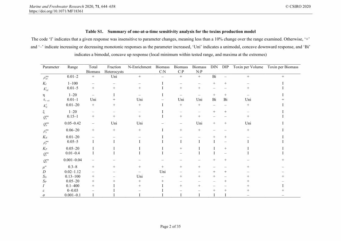
Table S1 summarises results of the one-at-a-time sensitivity analysis for the toxins production model.

Responses apart from toxins concentrations agreed with those previously found for the base model.

Variation in the two parameters governing toxins production (ε and σ) had interactive effects on toxins

concentrations (Fig. S1). Other predicted responses showed no strong interactions and displayed the

same responses found in the one-at-a-time sensitivity analysis.


of 35

Table S1. Summary of one-at-a-time sensitivity analysis for the toxins production model

The code ‘I’ indicates that a given response was insensitive to parameter changes, meaning less than a 10% change over the range examined. Otherwise, ‘+’

and ‘–’ indicate increasing or decreasing monotonic responses as the parameter increased, ‘Uni’ indicates a unimodal, concave downward response, and ‘Bi’

indicates a bimodal, concave up response (local minimum within tested range, and maxima at the extremes)

Parameter Range Total Biomass

Fraction Heterocysts

N-Enrichment Biomass C:N

Biomass C:P

Biomass N:P

DIN DIP Toxin per Volume Toxin per Biomass

maxNFρ 0.01–2 + Uni + – + + Bi – + +

KI 1–100 – – – I – – + + – I iNFK 0.01–5 + + + I + + – – + I

η 1–20 – I – I – – + + – I V Hk → 0.01–1 Uni + Uni – Uni Uni Bi Bi Uni +

IHK 0.01–20 + + + I + + – – + I

ξ 1–20 – – – I – – + + – I maxNQ 0.15–1 + + + I + + – – + I

minNQ 0.05–0.42 – Uni Uni – – Uni + + Uni I

maxNρ 0.06–20 + + + I + + – – + I

KN 0.01–20 – – – I – – + + – I maxPρ 0.05–5 I I I I I I I – I I

KP 0.05–20 I I I I + I I + I I maxPQ 0.01–0.4 I I I I – I I – I I

minPQ 0.001–0.04 – – – – – – + + – +

μ∞ 0.3–8 + + + + + + – – + – D 0.02–1.12 – – – Uni – – + + – – SN 0.13–100 + – Uni – + + + – + + SP 0.05–20 + + + + – – – + + – I 0.1–400 + I + I + + – – + I ε 0–0.03 – I – I – – + + + + σ 0.001–0.1 I I I I I I I I – –


of 35

Fig. S1. Concentrations of toxins v. the toxins production coefficient (ε, day–1) and toxins stoichiometry (σ,

μmol N μmol toxin–1): (a) Concentration per unit volume (μg L–1); (b) Concentration per unit biomass (μg mg

DW–1).

MATLAB scripts

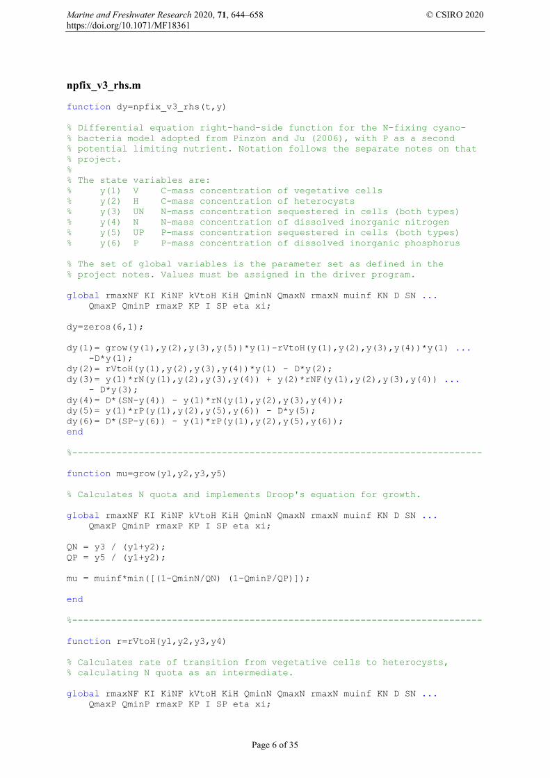
All scripts used a common function encoding equation system (6) for use with the MATLAB solvers

for ordinary differential equation. Scripts for the toxins production model additionally encode Eqn 7

and 8. For the base model, the file npfix_v3_rhs.m has one main function with four sub-functions that

encode the physiological rate functions μ(QN,QP), rV→H(QN,N), rNF(QN,I,N), rN(N,QN), rP(N,QP).

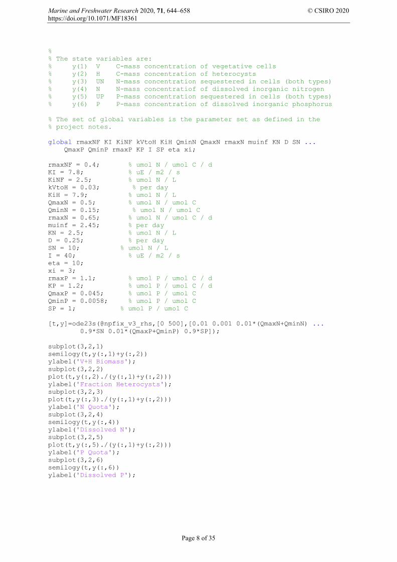
Driver scripts calling the solver ode23s and the npfix_v3_rhs function file were written to accomplish

various simulation tasks for the study. The script npfix_driver.m performs a single run of the model.

The script npfix_oat_driver.m performs a one-at-a-time sensitivity analysis with multiple runs. General

parameter assignments are made first, then particular lines of code must be rewritten to select one

parameter to vary, and its bounds. Simulations are then obtained for thirty linearly spaced values, and

summary plots are constructed for the output.

(a)

(b)


of 35

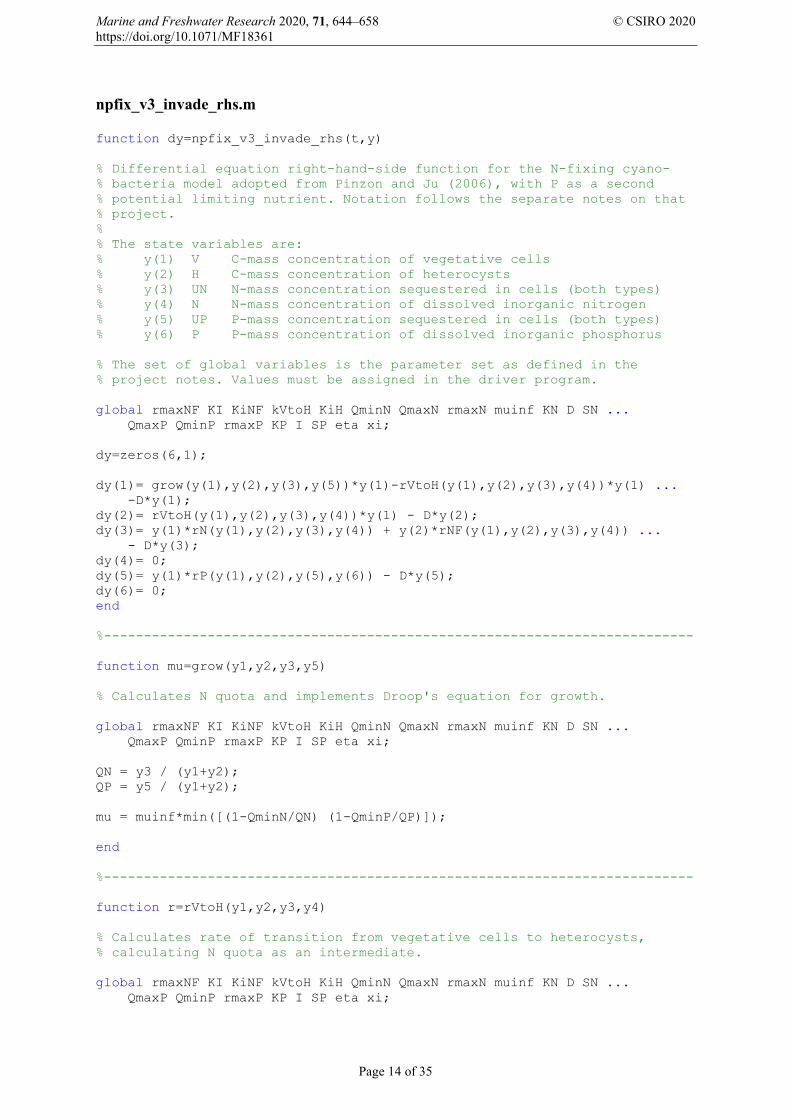
The script npfix_pip_driver.m constructs one pairwise-invasion-plot. General parameter assignments

are made first, then a grid of resident and invader (mutant) values of the parameter kV→H is defined. For

each of these values, resident dynamics are simulated for 1,000 days. Using results from these

simulations, an invasion phase of 50 days proceeds using the kV→H value for the mutant. This invasion

simulation uses a modified version of the npfix_v3_rhs function, the file npfix_v3_invade_rhs.m, in

which the derivatives for N and P dynamics are set to zero, so that the concentrations of DIN and DIP

remain at the equilibrium values determined by the resident’s phenotype. The last two time intervals

reported by the ode23s solver are then used to calculate the net growth rate of the mutant population.

Positive rates are plotted as black pixels on the pairwise-invasion-plot graph.

For the toxins production model, the file npfixtox_rhs.m has one main function that encodes the base

model and its functions along with Eqn 7 and 8. Driver scripts calling the solver ode23s and the

npfixtox_rhs function file were written to accomplish various simulation tasks for the study.

The script npfixtox_driver.m performs a single run of the model. The script npfixtox_oat_driver.m

performs a one-at-a-time sensitivity analysis with multiple runs. General parameter assignments are

made first, then particular lines of code must be rewritten to select one parameter to vary, and its bounds.

Simulations are then obtained for thirty linearly spaced values, and summary plots are constructed for

the output.

The script npfixtox_esgrid_driver.m obtains the output used to construct predictions in relation to

the toxins parameters ε and σ, producing the graphs shown in Fig. S1. General parameter assignments

are made first, and a grid of 30 × 30 linearly spaced values of ε and σ is created. Then 900 simulations

run and results are graphed.

The script npfixtox_supply_driver.m obtains the output used to construct the graphs shown in Fig. 6.

General parameter assignments are made first, and a grid of 31 × 31 linearly spaced values of SN and SP

is created. Then 961 simulations run for the array of supply points. In using this program to construct

the results reported, the lowest of the 31 assigned supply values for DIN and DIP often produced extinct

populations (and some attendant numerical artefacts). Results from these supply points were discarded,

leaving the 30 × 30 grid reported in the main text. After trimming away these points, the program plots

results. Fig. 5d was made manually from saved results.

The script npfixtox_rand_driver.m obtains the output used to construct the graphs shown in Fig. 6a–

d. Triangular distributions are made for each parameter are made first and then a loop is executed

making parameter assignments by generating random numbers from these distributions. After random

parameter assignments at the beginning of this loop, there is a check to see whether the parameter maxNQ

is at least twice maxNQ . If not, another parameter set is assigned with new random numbers. A simulation

executes if parameter values are acceptable. After this simulation, results are accepted if: (1) the change


of 35

in total biomass during the last time step reported by the ode23s solver is sufficiently small, indicating

convergence to equilibrium; (2) total biomass at the end of the run is large enough to be consistent with

a persistent population; and (3) the proportion of biomass represented by heterocysts is < 25%. When

results are not acceptable by this criterion, the loop is repeated with a new random parameter set. The

loop is repeated until 1000 acceptable results are obtained. The script npfixtox_randenv_driver.m

obtains the output used to construct the graphs shown in Fig. 6e–h. It is identical to

npfixtox_rand_driver.m, which randomises all parameter assignments, except that after making random

assignments all parameters are overwritten by default values, except for the environmental parameters

D, I, SN, and SP. In this way, only the latter parameters are assigned at random. However, both scripts

for random parameter assignments make the same number of calls to the random number generator, so

that when the same seed is used for the generator, the scripts use the same sequence of random numbers

for parameter assignments.


of 35

npfix_v3_rhs.m function dy=npfix_v3_rhs(t,y) % Differential equation right-hand-side function for the N-fixing cyano- % bacteria model adopted from Pinzon and Ju (2006), with P as a second % potential limiting nutrient. Notation follows the separate notes on that % project. % % The state variables are: % y(1) V C-mass concentration of vegetative cells % y(2) H C-mass concentration of heterocysts % y(3) UN N-mass concentration sequestered in cells (both types) % y(4) N N-mass concentration of dissolved inorganic nitrogen % y(5) UP P-mass concentration sequestered in cells (both types) % y(6) P P-mass concentration of dissolved inorganic phosphorus % The set of global variables is the parameter set as defined in the % project notes. Values must be assigned in the driver program. global rmaxNF KI KiNF kVtoH KiH QminN QmaxN rmaxN muinf KN D SN ... QmaxP QminP rmaxP KP I SP eta xi; dy=zeros(6,1); dy(1)= grow(y(1),y(2),y(3),y(5))*y(1)-rVtoH(y(1),y(2),y(3),y(4))*y(1) ... -D*y(1); dy(2)= rVtoH(y(1),y(2),y(3),y(4))*y(1) - D*y(2); dy(3)= y(1)*rN(y(1),y(2),y(3),y(4)) + y(2)*rNF(y(1),y(2),y(3),y(4)) ... - D*y(3); dy(4)= D*(SN-y(4)) - y(1)*rN(y(1),y(2),y(3),y(4)); dy(5)= y(1)*rP(y(1),y(2),y(5),y(6)) - D*y(5); dy(6)= D*(SP-y(6)) - y(1)*rP(y(1),y(2),y(5),y(6)); end %-------------------------------------------------------------------------- function mu=grow(y1,y2,y3,y5) % Calculates N quota and implements Droop's equation for growth. global rmaxNF KI KiNF kVtoH KiH QminN QmaxN rmaxN muinf KN D SN ... QmaxP QminP rmaxP KP I SP eta xi; QN = y3 / (y1+y2); QP = y5 / (y1+y2); mu = muinf*min([(1-QminN/QN) (1-QminP/QP)]); end %-------------------------------------------------------------------------- function r=rVtoH(y1,y2,y3,y4) % Calculates rate of transition from vegetative cells to heterocysts, % calculating N quota as an intermediate. global rmaxNF KI KiNF kVtoH KiH QminN QmaxN rmaxN muinf KN D SN ... QmaxP QminP rmaxP KP I SP eta xi;


of 35

QN = y3 / (y1+y2); r = kVtoH*((QmaxN-QN)/(QmaxN-QminN))^xi*(KiH/(KiH+y4)); end %-------------------------------------------------------------------------- function r=rN(y1,y2,y3,y4) % Calculates N uptake rate using Thingstad's formula. global rmaxNF KI KiNF kVtoH KiH QminN QmaxN rmaxN muinf KN D SN ... QmaxP QminP rmaxP KP I SP eta xi; QN = y3 / (y1+y2); r = rmaxN*((QmaxN-QN)/(QmaxN-QminN))*(y4/(KN+y4)); end %-------------------------------------------------------------------------- function r=rNF(y1,y2,y3,y4) % Calculates rate of N-fixation. global rmaxNF KI KiNF kVtoH KiH QminN QmaxN rmaxN muinf KN D SN ... QmaxP QminP rmaxP KP I SP eta xi; QN = y3 / (y1+y2); r = rmaxNF*((QmaxN-QN)/(QmaxN-QminN))^eta*(I/(KI+I))*(KiNF/(KiNF+y4)); end %-------------------------------------------------------------------------- function r=rP(y1,y2,y5,y6) % Calculates N uptake rate using Thingstad's formula. global rmaxNF KI KiNF kVtoH KiH QminN QmaxN rmaxN muinf KN D SN ... QmaxP QminP rmaxP KP I SP eta xi; QP = y5 / (y1+y2); r = rmaxP*((QmaxP-QP)/(QmaxP-QminP))*(y6/(KP+y6)); end %-------------------------------------------------------------------------- npfix_driver.m close all; clear all; % Differential equation driver for the N-fixing cyano- % bacteria model adopted from Pinzon and Ju (2006). % Notation follows the separate notes on that project.


of 35

% % The state variables are: % y(1) V C-mass concentration of vegetative cells % y(2) H C-mass concentration of heterocysts % y(3) UN N-mass concentration sequestered in cells (both types) % y(4) N N-mass concentratiof of dissolved inorganic nitrogen % y(5) UP P-mass concentration sequestered in cells (both types) % y(6) P P-mass concentration of dissolved inorganic phosphorus % The set of global variables is the parameter set as defined in the % project notes. global rmaxNF KI KiNF kVtoH KiH QminN QmaxN rmaxN muinf KN D SN ... QmaxP QminP rmaxP KP I SP eta xi; rmaxNF = 0.4; % umol N / umol C / d KI = 7.8; % uE / m2 / s KiNF = 2.5; % umol N / L kVtoH = 0.03; % per day KiH = 7.9; % umol N / L QmaxN = 0.5; % umol N / umol C QminN = 0.15; % umol N / umol C rmaxN = 0.65; % umol N / umol C / d muinf = 2.45; % per day KN = 2.5; % umol N / L D = 0.25; % per day SN = 10; % umol N / L I = 40; % uE / m2 / s eta = 10; xi = 3; rmaxP = 1.1; % umol P / umol C / d KP = 1.2; % umol P / umol C / d QmaxP = 0.045; % umol P / umol C QminP = 0.0058; % umol P / umol C SP = 1; % umol P / umol C [t,y]=ode23s(@npfix_v3_rhs,[0 500],[0.01 0.001 0.01*(QmaxN+QminN) ... 0.9*SN 0.01*(QmaxP+QminP) 0.9*SP]); subplot(3,2,1) semilogy(t,y(:,1)+y(:,2)) ylabel('V+H Biomass'); subplot(3,2,2) plot(t,y(:,2)./(y(:,1)+y(:,2))) ylabel('Fraction Heterocysts'); subplot(3,2,3) plot(t,y(:,3)./(y(:,1)+y(:,2))) ylabel('N Quota'); subplot(3,2,4) semilogy(t,y(:,4)) ylabel('Dissolved N'); subplot(3,2,5) plot(t,y(:,5)./(y(:,1)+y(:,2))) ylabel('P Quota'); subplot(3,2,6) semilogy(t,y(:,6)) ylabel('Dissolved P');


of 35

npfix_oat_driver.m

close all; clear all; % Differential equation driver for the N-fixing cyano- % bacteria model adopted from Pinzon and Ju (2006). % Notation follows the separate notes on that project. % % The state variables are: % y(1) V C-mass concentration of vegetative cells % y(2) H C-mass concentration of heterocysts % y(3) UN N-mass concentration sequestered in cells (both types) % y(4) N N-mass concentratiof of dissolved inorganic nitrogen % y(5) UP P-mass concentration sequestered in cells (both types) % y(6) P P-mass concentration of dissolved inorganic phosphorus % The set of global variables is the parameter set as defined in the % project notes. % The driver implements a one-at-a-time sensitivity analysis % for a selected parameter. Particular lines of code must be % rewritten to do this. global rmaxNF KI KiNF kVtoH KiH QminN QmaxN rmaxN muinf KN D SN ... QmaxP QminP rmaxP KP I SP eta xi; rmaxNF = 0.4; % umol N / umol C / d KI = 7.8; % uE / m2 / s KiNF = 2.5; % umol N / L kVtoH = 0.03; % per day KiH = 7.9; % umol N / L QmaxN = 0.5; % umol N / umol C QminN = 0.15; % umol N / umol C rmaxN = 0.65; % umol N / umol C / d muinf = 2.45; % per day KN = 2.5; % umol N / L D = 0.25; % per day SN = 10.0; % umol N / L I = 40; % uE / m2 / s eta = 10; xi = 3; rmaxP = 1.1; % umol P / umol C / d KP = 1.2; % umol P / umol C / d QmaxP = 0.045; % umol P / umol C QminP = 0.0058; % umol P / umol C SP = 1.0; % umol P / umol C parmlo = 0.13; % Rewrite this line as needed parmhi = 100; % Rewrite this line as needed parm = linspace(parmlo,parmhi,30); V = zeros(1,30); H = zeros(1,30); UN = zeros(1,30); N = zeros(1,30); UP = zeros(1,30); P = zeros(1,30); Total = zeros(1,30); FHet = zeros(1,30);


of 35

CtoN = zeros(1,30); CtoP = zeros(1,30); NtoP = zeros(1,30); NEnrich = zeros(1,30); Change = zeros(1,30); for i=1:30 SN = parm(i); % Rewrite this line as needed [t,y]=ode23s(@npfix_v3_rhs,[0 1000],[0.01 0.01 0.01*(QmaxN+QminN) ... 0.9*SN 0.01*(QmaxP+QminP) 0.9*SP]); last = size(t); last = last(1); V(i) = y(last,1); H(i) = y(last,2); UN(i) = y(last,3); N(i) = y(last,4); UP(i) = y(last,5); P(i) = y(last,6); Total(i) = V(i)+H(i); FHet(i) = H(i)/(V(i)+H(i)); CtoN(i) = Total(i)/UN(i); CtoP(i) = Total(i)/UP(i); NtoP(i) = UN(i)/UP(i); NEnrich(i) = (UN(i)+N(i))/SN; PrevTotal = y(last-1,1)+y(last-1,2); Change(i) = (log(Total(i))-log(PrevTotal))/(t(last)-t(last-1)); end figure(1) subplot(3,3,1) plot(parm,Total) ylabel('Total Biomass'); subplot(3,3,2) plot(parm,FHet) ylabel('Fraction H'); subplot(3,3,3) plot(parm,NEnrich) ylabel('N Enrichment'); subplot(3,3,4) plot(parm,UN) ylabel('Biomass N'); subplot(3,3,5) plot(parm,UP) ylabel('Biomass P'); subplot(3,3,6) plot(parm,Change) ylabel('Rate of Change'); subplot(3,3,7) plot(parm,CtoN) ylabel('Population C:N'); subplot(3,3,8) plot(parm,CtoP) ylabel('Population C:P'); xlabel('SN'); % Rewrite this line as needed subplot(3,3,9) plot(parm,NtoP) ylabel('Population N:P'); figure(2) subplot(2,1,1) plot(parm,N)


of 35

ylabel('Dissolved N'); subplot(2,1,2) plot(parm,P) ylabel('Dissolved P'); xlabel('SN'); % Rewrite this line as needed


of 35

npfix_pip_driver.m

close all; clear all; % Differential equation driver for the N-fixing cyano- % bacteria model adopted from Pinzon and Ju (2006). % Notation follows the separate notes on that project. % % The state variables are: % y(1) V C-mass concentration of vegetative cells % y(2) H C-mass concentration of heterocysts % y(3) UN N-mass concentration sequestered in cells (both types) % y(4) N N-mass concentratiof of dissolved inorganic nitrogen % y(5) UP P-mass concentration sequestered in cells (both types) % y(6) P P-mass concentration of dissolved inorganic phosphorus % The set of global variables is the parameter set as defined in the % project notes. % The driver creates a pairwise-invasion-plot for a parameter representing % a trait of N-fixing cyanobacteria. An array of resident and invader % traits are tested to build up the PIP. For each point the establishment- % invasion protocol of the single invasion scenario driver is used. % Rates of invasion (fitness) are calculated from the last and last-2 % biomass data points. These and the associated time intervals are % recorded. global rmaxNF KI KiNF kVtoH KiH QminN QmaxN rmaxN muinf KN D SN ... QmaxP QminP rmaxP KP I SP eta xi; rmaxNF = 0.4; % umol N / umol C / d KI = 7.8; % uE / m2 / s KiNF = 2.5; % umol N / L kVtoH = 0.03; % per day KiH = 7.9; % umol N / L QmaxN = 0.5; % umol N / umol C QminN = 0.15; % umol N / umol C rmaxN = 0.65; % umol N / umol C / d muinf = 2.45; % per day KN = 2.5; % umol N / L D = 0.25; % per day I = 40; % uE / m2 / s eta = 10; xi = 3; rmaxP = 1.1; % umol P / umol C / d KP = 1.2; % umol P / umol C / d QmaxP = 0.045; % umol P / umol C QminP = 0.0058; % umol P / umol C SN = 100; % umol N / L SP = 10; % umol P / umol C GridSize = 50; count=0; Rate = zeros(GridSize); Time = zeros(GridSize); ResTrait = linspace(0,0.15,GridSize); InvTrait = linspace(0,0.15,GridSize);


of 35

for i=1:GridSize for j=1:GridSize kVtoH = ResTrait(i); [t,y]=ode23s(@npfix_v3_rhs,[0 1000],[0.01 0.001 ... 0.01*(QminN+QmaxN) 0.9*SN 0.01*(QminP+QmaxP) 0.9*SP]); last = size(t); last = last(1); N = y(last,4); P = y(last,6); kVtoH = InvTrait(j); [t,y]=ode23s(@npfix_v3_invade_rhs,[0 50],[0.01 0.001 ... 0.01*(QminN+QmaxN) N 0.01*(QminP+QmaxP) P]); last = size(t); last = last(1); Time(i,j) = t(last)-t(last-2); Rate(i,j) = (log(y(last,1)+y(last,2)) - log(y(last-2,1)+ ... y(last-2,2)))/Time(i,j); if Rate(i,j) > 0 figure(1) plot(ResTrait(i),InvTrait(j),'ks','MarkerFaceColor','k') hold on end count=count+1 end end figure(1) axis square xlabel('Resident Trait') ylabel('Invader Trait') TimeRange = [min(min(Time)) max(max(Time))]


of 35

npfix_v3_invade_rhs.m

function dy=npfix_v3_invade_rhs(t,y) % Differential equation right-hand-side function for the N-fixing cyano- % bacteria model adopted from Pinzon and Ju (2006), with P as a second % potential limiting nutrient. Notation follows the separate notes on that % project. % % The state variables are: % y(1) V C-mass concentration of vegetative cells % y(2) H C-mass concentration of heterocysts % y(3) UN N-mass concentration sequestered in cells (both types) % y(4) N N-mass concentration of dissolved inorganic nitrogen % y(5) UP P-mass concentration sequestered in cells (both types) % y(6) P P-mass concentration of dissolved inorganic phosphorus % The set of global variables is the parameter set as defined in the % project notes. Values must be assigned in the driver program. global rmaxNF KI KiNF kVtoH KiH QminN QmaxN rmaxN muinf KN D SN ... QmaxP QminP rmaxP KP I SP eta xi; dy=zeros(6,1); dy(1)= grow(y(1),y(2),y(3),y(5))*y(1)-rVtoH(y(1),y(2),y(3),y(4))*y(1) ... -D*y(1); dy(2)= rVtoH(y(1),y(2),y(3),y(4))*y(1) - D*y(2); dy(3)= y(1)*rN(y(1),y(2),y(3),y(4)) + y(2)*rNF(y(1),y(2),y(3),y(4)) ... - D*y(3); dy(4)= 0; dy(5)= y(1)*rP(y(1),y(2),y(5),y(6)) - D*y(5); dy(6)= 0; end %-------------------------------------------------------------------------- function mu=grow(y1,y2,y3,y5) % Calculates N quota and implements Droop's equation for growth. global rmaxNF KI KiNF kVtoH KiH QminN QmaxN rmaxN muinf KN D SN ... QmaxP QminP rmaxP KP I SP eta xi; QN = y3 / (y1+y2); QP = y5 / (y1+y2); mu = muinf*min([(1-QminN/QN) (1-QminP/QP)]); end %-------------------------------------------------------------------------- function r=rVtoH(y1,y2,y3,y4) % Calculates rate of transition from vegetative cells to heterocysts, % calculating N quota as an intermediate. global rmaxNF KI KiNF kVtoH KiH QminN QmaxN rmaxN muinf KN D SN ... QmaxP QminP rmaxP KP I SP eta xi;


of 35

QN = y3 / (y1+y2); r = kVtoH*((QmaxN-QN)/(QmaxN-QminN))^xi*(KiH/(KiH+y4)); end %-------------------------------------------------------------------------- function r=rN(y1,y2,y3,y4) % Calculates N uptake rate using Thingstad's formula. global rmaxNF KI KiNF kVtoH KiH QminN QmaxN rmaxN muinf KN D SN ... QmaxP QminP rmaxP KP I SP eta xi; QN = y3 / (y1+y2); r = rmaxN*((QmaxN-QN)/(QmaxN-QminN))*(y4/(KN+y4)); end %-------------------------------------------------------------------------- function r=rNF(y1,y2,y3,y4) % Calculates rate of N-fixation. global rmaxNF KI KiNF kVtoH KiH QminN QmaxN rmaxN muinf KN D SN ... QmaxP QminP rmaxP KP I SP eta xi; QN = y3 / (y1+y2); r = rmaxNF*((QmaxN-QN)/(QmaxN-QminN))^eta*(I/(KI+I))*(KiNF/(KiNF+y4)); end %-------------------------------------------------------------------------- function r=rP(y1,y2,y5,y6) % Calculates N uptake rate using Thingstad's formula. global rmaxNF KI KiNF kVtoH KiH QminN QmaxN rmaxN muinf KN D SN ... QmaxP QminP rmaxP KP I SP eta xi; QP = y5 / (y1+y2); r = rmaxP*((QmaxP-QP)/(QmaxP-QminP))*(y6/(KP+y6)); end %-------------------------------------------------------------------------- npfixtox_rhs.m

function dy=npfixtox_rhs(t,y) % Differential equation right-hand-side function for the N-fixing cyano- % bacteria model adopted from Pinzon and Ju (2006), with P as a second % potential limiting nutrient. Toxin production is added to previous % model versions. Notation follows the separate notes on the project. %


of 35

% The state variables are: % y(1) V C-mass concentration of vegetative cells % y(2) H C-mass concentration of heterocysts % y(3) UN N-mass concentration sequestered in cells (both types) % y(4) N N-mass concentration of dissolved inorganic nitrogen % y(5) UP P-mass concentration sequestered in cells (both types) % y(6) P P-mass concentration of dissolved inorganic phosphorus % y(7) C mass concentration of toxin % The set of global variables is the parameter set as defined in the % project notes. Values must be assigned in the driver program. global rmaxNF KI KiNF kVtoH KiH QminN QmaxN rmaxN muinf KN D SN ... QmaxP QminP rmaxP KP I SP eta xi epsilon sigma; dy=zeros(7,1); dy(1)= grow(y(1),y(2),y(3),y(5))*y(1)-rVtoH(y(1),y(2),y(3),y(4))*y(1) ... -D*y(1); dy(2)= rVtoH(y(1),y(2),y(3),y(4))*y(1) - D*y(2); dy(3)= y(1)*rN(y(1),y(2),y(3),y(4)) + y(2)*rNF(y(1),y(2),y(3),y(4)) ... - (D+epsilon)*y(3); dy(4)= D*(SN-y(4)) - y(1)*rN(y(1),y(2),y(3),y(4)); dy(5)= y(1)*rP(y(1),y(2),y(5),y(6)) - D*y(5); dy(6)= D*(SP-y(6)) - y(1)*rP(y(1),y(2),y(5),y(6)); dy(7)= epsilon*y(3)/sigma-D*y(7); end %-------------------------------------------------------------------------- function mu=grow(y1,y2,y3,y5) % Calculates N quota and implements Droop's equation for growth. global rmaxNF KI KiNF kVtoH KiH QminN QmaxN rmaxN muinf KN D SN ... QmaxP QminP rmaxP KP I SP eta xi; QN = y3 / (y1+y2); QP = y5 / (y1+y2); mu = muinf*min([(1-QminN/QN) (1-QminP/QP)]); end %-------------------------------------------------------------------------- function r=rVtoH(y1,y2,y3,y4) % Calculates rate of transition from vegetative cells to heterocysts, % calculating N quota as an intermediate. global rmaxNF KI KiNF kVtoH KiH QminN QmaxN rmaxN muinf KN D SN ... QmaxP QminP rmaxP KP I SP eta xi; QN = y3 / (y1+y2); r = kVtoH*((QmaxN-QN)/(QmaxN-QminN))^xi*(KiH/(KiH+y4)); end


of 35

%-------------------------------------------------------------------------- function r=rN(y1,y2,y3,y4) % Calculates N uptake rate using Thingstad's formula. global rmaxNF KI KiNF kVtoH KiH QminN QmaxN rmaxN muinf KN D SN ... QmaxP QminP rmaxP KP I SP eta xi; QN = y3 / (y1+y2); r = rmaxN*((QmaxN-QN)/(QmaxN-QminN))*(y4/(KN+y4)); end %-------------------------------------------------------------------------- function r=rNF(y1,y2,y3,y4) % Calculates rate of N-fixation. global rmaxNF KI KiNF kVtoH KiH QminN QmaxN rmaxN muinf KN D SN ... QmaxP QminP rmaxP KP I SP eta xi; QN = y3 / (y1+y2); r = rmaxNF*((QmaxN-QN)/(QmaxN-QminN))^eta*(I/(KI+I))*(KiNF/(KiNF+y4)); end %-------------------------------------------------------------------------- function r=rP(y1,y2,y5,y6) % Calculates N uptake rate using Thingstad's formula. global rmaxNF KI KiNF kVtoH KiH QminN QmaxN rmaxN muinf KN D SN ... QmaxP QminP rmaxP KP I SP eta xi; QP = y5 / (y1+y2); r = rmaxP*((QmaxP-QP)/(QmaxP-QminP))*(y6/(KP+y6)); end %--------------------------------------------------------------------------


of 35

npfixtox_driver.m close all; clear all; % Differential equation driver for the N-fixing cyano- % bacteria model adopted from Pinzon and Ju (2006). Toxin production is % added to previous model versions. Notation follows the separate notes % on the project. % % The state variables are: % y(1) V C-mass concentration of vegetative cells % y(2) H C-mass concentration of heterocysts % y(3) UN N-mass concentration sequestered in cells (both types) % y(4) N N-mass concentratiof of dissolved inorganic nitrogen % y(5) UP P-mass concentration sequestered in cells (both types) % y(6) P P-mass concentration of dissolved inorganic phosphorus % y(7) C mass concentration of toxin % The set of global variables is the parameter set as defined in the % project notes. global rmaxNF KI KiNF kVtoH KiH QminN QmaxN rmaxN muinf KN D SN ... QmaxP QminP rmaxP KP I SP eta xi epsilon sigma; rmaxNF = 0.4; % umol N / umol C / d KI = 7.8; % uE / m2 / s KiNF = 2.5; % umol N / L kVtoH = 0.03; % per day KiH = 7.9; % umol N / L QmaxN = 0.5; % umol N / umol C QminN = 0.15; % umol N / umol C rmaxN = 0.65; % umol N / umol C / d muinf = 2.45; % per day KN = 2.5; % umol N / L D = 0.25; % per day SN = 10; % umol N / L I = 40; % uE / m2 / s eta = 10; xi = 3; rmaxP = 1.1; % umol P / umol C / d KP = 1.2; % umol P / umol C / d QmaxP = 0.045; % umol P / umol C QminP = 0.0058; % umol P / umol C SP = 1; % umol P / umol C epsilon = 0.002; % per day sigma = 0.023; % umol N / ug toxin [t,y]=ode23s(@npfixtox_rhs,[0 500],[0.01 0.001 0.01*(QmaxN+QminN) ... 0.9*SN 0.01*(QmaxP+QminP) 0.9*SP 0]); subplot(3,3,1) semilogy(t,y(:,1)+y(:,2)) ylabel('V+H Biomass'); subplot(3,3,2) plot(t,y(:,2)./(y(:,1)+y(:,2))) ylabel('Fraction H'); subplot(3,3,3) plot(t,y(:,3)./(y(:,1)+y(:,2))) ylabel('N Quota'); subplot(3,3,4)


of 35

semilogy(t,y(:,4)) ylabel('Dissolved N'); subplot(3,3,5) plot(t,y(:,5)./(y(:,1)+y(:,2))) ylabel('P Quota'); subplot(3,3,6) semilogy(t,y(:,6)) ylabel('Dissolved P'); % This plot shows toxin concentration as ug toxin / L subplot(3,3,7) semilogy(t,y(:,7)) ylabel('Toxin'); % This plot shows toxin concentration as ug toxin / mg DW subplot(3,3,8) semilogy( t,y(:,7)*1000*0.5 ./ ((y(:,1)+y(:,2))*12) ) ylabel('Toxin (ug / mg DW)');


of 35

npfixtox_oat_driver.m close all; clear all; % Differential equation driver for the N-fixing cyano- % bacteria model adopted from Pinzon and Ju (2006). Toxin production is % added to previous model versions. Notation follows the separate notes % on the project. % % The state variables are: % y(1) V C-mass concentration of vegetative cells % y(2) H C-mass concentration of heterocysts % y(3) UN N-mass concentration sequestered in cells (both types) % y(4) N N-mass concentratiof of dissolved inorganic nitrogen % y(5) UP P-mass concentration sequestered in cells (both types) % y(6) P P-mass concentration of dissolved inorganic phosphorus % y(7) C mass concentration of toxin % The set of global variables is the parameter set as defined in the % project notes. % The driver implements a one-at-a-time sensitivity analysis % for a selected parameter. Particular lines of code must be % rewritten to do this. global rmaxNF KI KiNF kVtoH KiH QminN QmaxN rmaxN muinf KN D SN ... QmaxP QminP rmaxP KP I SP eta xi epsilon sigma; rmaxNF = 0.4; % umol N / umol C / d KI = 7.8; % uE / m2 / s KiNF = 2.5; % umol N / L kVtoH = 0.03; % per day KiH = 7.9; % umol N / L QmaxN = 0.5; % umol N / umol C QminN = 0.15; % umol N / umol C rmaxN = 0.65; % umol N / umol C / d muinf = 2.45; % per day KN = 2.5; % umol N / L D = 0.25; % per day SN = 10.0; % umol N / L I = 40; % uE / m2 / s eta = 10; xi = 3; rmaxP = 1.1; % umol P / umol C / d KP = 1.2; % umol P / umol C / d QmaxP = 0.045; % umol P / umol C QminP = 0.0058; % umol P / umol C SP = 1.0; % umol P / umol C epsilon = 0.002; % per day sigma = 0.023; % umol N / ug toxin parmlo = 0.001; % Rewrite this line as needed parmhi = 0.1; % Rewrite this line as needed parm = linspace(parmlo,parmhi,30); V = zeros(1,30); H = zeros(1,30); UN = zeros(1,30); N = zeros(1,30);


of 35

UP = zeros(1,30); P = zeros(1,30); Total = zeros(1,30); FHet = zeros(1,30); CtoN = zeros(1,30); CtoP = zeros(1,30); NtoP = zeros(1,30); NEnrich = zeros(1,30); Change = zeros(1,30); for i=1:30 sigma = parm(i); % Rewrite this line as needed [t,y]=ode23s(@npfixtox_rhs,[0 1000],[0.01 0.01 0.01*(QmaxN+QminN) ... 0.9*SN 0.01*(QmaxP+QminP) 0.9*SP 0]); last = size(t); last = last(1); V(i) = y(last,1); H(i) = y(last,2); UN(i) = y(last,3); N(i) = y(last,4); UP(i) = y(last,5); P(i) = y(last,6); C(i) = y(last,7); Total(i) = V(i)+H(i); FHet(i) = H(i)/(V(i)+H(i)); CtoN(i) = Total(i)/UN(i); CtoP(i) = Total(i)/UP(i); NtoP(i) = UN(i)/UP(i); NEnrich(i) = (UN(i)+N(i))/SN; ToxDW(i) = C(i)*1000*0.5/(12*Total(i)); % Toxin ug per mg Dry Weight ToxN(i) = C(i)*sigma/UN(i); % Toxin N as fraction of cell N PrevTotal = y(last-1,1)+y(last-1,2); Change(i) = (log(Total(i))-log(PrevTotal))/(t(last)-t(last-1)); end figure(1) subplot(2,3,1) plot(parm,Total) ylabel('Total Biomass'); subplot(2,3,2) plot(parm,FHet) ylabel('Fraction H'); subplot(2,3,3) plot(parm,Change) ylabel('Rate of Change'); subplot(2,3,4) plot(parm,NEnrich) ylabel('N Enrichment'); subplot(2,3,5) plot(parm,N) ylabel('DIN'); xlabel('sigma'); % Rewrite this line as needed subplot(2,3,6) plot(parm,P) ylabel('DIP'); figure(2) subplot(2,3,1) plot(parm,CtoN) ylabel('Population C:N'); subplot(2,3,2)


of 35

plot(parm,CtoP) ylabel('Population C:P'); subplot(2,3,3) plot(parm,NtoP) ylabel('Population N:P'); subplot(2,3,4) plot(parm,C) ylabel('Toxin per L'); subplot(2,3,5) plot(parm,ToxDW) ylabel('Toxin per DW'); xlabel('sigma'); % Rewrite this line as needed subplot(2,3,6) plot(parm,ToxN) ylabel('Toxin Cell N');


of 35

npfixtox_esgrid_driver close all; clear all; % Differential equation driver for the N-fixing cyano- % bacteria model adopted from Pinzon and Ju (2006). Toxin production is % added to previous model versions. Notation follows the separate notes % on the project. % % The state variables are: % y(1) V C-mass concentration of vegetative cells % y(2) H C-mass concentration of heterocysts % y(3) UN N-mass concentration sequestered in cells (both types) % y(4) N N-mass concentratiof of dissolved inorganic nitrogen % y(5) UP P-mass concentration sequestered in cells (both types) % y(6) P P-mass concentration of dissolved inorganic phosphorus % y(7) C mass concentration of toxin % The set of global variables is the parameter set as defined in the % project notes. % The driver implements runs over a grid of the parameters epsilon % and sigma, which govern toxin production and properties. global rmaxNF KI KiNF kVtoH KiH QminN QmaxN rmaxN muinf KN D SN ... QmaxP QminP rmaxP KP I SP eta xi epsilon sigma; rmaxNF = 0.4; % umol N / umol C / d KI = 7.8; % uE / m2 / s KiNF = 2.5; % umol N / L kVtoH = 0.03; % per day KiH = 7.9; % umol N / L QmaxN = 0.5; % umol N / umol C QminN = 0.15; % umol N / umol C rmaxN = 0.65; % umol N / umol C / d muinf = 2.45; % per day KN = 2.5; % umol N / L D = 0.25; % per day SN = 10.0; % umol N / L I = 40; % uE / m2 / s eta = 10; xi = 3; rmaxP = 1.1; % umol P / umol C / d KP = 1.2; % umol P / umol C / d QmaxP = 0.045; % umol P / umol C QminP = 0.0058; % umol P / umol C SP = 1.0; % umol P / umol C epsilon = 0.002; % per day sigma = 0.023; % umol N / ug toxin EpsilonGrid = zeros(30); SigmaGrid = zeros(30); V = zeros(30); H = zeros(30); UN = zeros(30); N = zeros(30); UP = zeros(30); P = zeros(30); C = zeros(30); Total = zeros(30);


of 35

FHet = zeros(30); QN = zeros(30); QP = zeros(30); CtoN = zeros(30); CtoP = zeros(30); NtoP = zeros(30); NEnrich = zeros(30); ToxDW = zeros(30); ToxN = zeros(30); Change = zeros(30); count = 0; EpsilonLo = 0; EpsilonHi = 0.01; SigmaLo = 0.006; SigmaHi = 0.023; EpsilonAxis = linspace(EpsilonLo,EpsilonHi,30); SigmaAxis = linspace(SigmaLo,SigmaHi,30); for i=1:30 for j=1:30 epsilon = EpsilonAxis(i); sigma = SigmaAxis(j); [t,y]=ode23s(@npfixtox_rhs,[0 1000],[0.01 0.01 0.01*(QmaxN+QminN) ... 0.9*SN 0.01*(QmaxP+QminP) 0.9*SP 0]); last = size(t); last = last(1); EpsilonGrid(i,j) = epsilon; SigmaGrid(i,j) = sigma; V(i,j) = y(last,1); H(i,j) = y(last,2); UN(i,j) = y(last,3); N(i,j) = y(last,4); UP(i,j) = y(last,5); P(i,j) = y(last,6); C(i,j) = y(last,7); Total(i,j) = V(i,j)+H(i,j); FHet(i,j) = H(i,j)/(V(i,j)+H(i,j)); QN(i,j) = (UN(i,j)/Total(i,j)-QminN)/(QmaxN-QminN); QP(i,j) = (UP(i,j)/Total(i,j)-QminP)/(QmaxP-QminP); CtoN(i,j) = Total(i,j)/UN(i,j); CtoP(i,j) = Total(i,j)/UP(i,j); NtoP(i,j) = UN(i,j)/UP(i,j); NEnrich(i,j) = (UN(i,j)+N(i,j))/SN; ToxDW(i,j) = C(i,j)*1000*0.5/(12*Total(i,j)); ToxN(i,j) = C(i,j)*sigma/UN(i,j); PrevTotal = y(last-1,1)+y(last-1,2); Change(i,j) = (log(Total(i,j))-log(PrevTotal))/(t(last)-t(last-1)); count = count+1; count end end figure(1) surf(SigmaAxis,EpsilonAxis,Total) ylabel('epsilon') xlabel('sigma') zlabel('Total Biomass') figure(2)


of 35

surf(SigmaAxis,EpsilonAxis,FHet) ylabel('epsilon') xlabel('sigma') zlabel('Fraction H') figure(3) surf(SigmaAxis,EpsilonAxis,CtoN) ylabel('epsilon') xlabel('sigma') zlabel('Biomass C:N') figure(4) surf(SigmaAxis,EpsilonAxis,CtoP) ylabel('epsilon') xlabel('sigma') zlabel('Biomass C:P') figure(5) surf(SigmaAxis,EpsilonAxis,NtoP) ylabel('epsilon') xlabel('sigma') zlabel('Biomass N:P') figure(6) surf(SigmaAxis,EpsilonAxis,NEnrich) ylabel('epsilon') xlabel('sigma') zlabel('NEnrichment') figure(7) surf(SigmaAxis,EpsilonAxis,C) ylabel('epsilon') xlabel('sigma') zlabel('Toxin per Liter') figure(8) surf(SigmaAxis,EpsilonAxis,ToxDW) ylabel('epsilon') xlabel('sigma') zlabel('Toxin per Biomass') figure(9) surf(SigmaAxis,EpsilonAxis,ToxN) ylabel('epsilon') xlabel('sigma') zlabel('Toxin Cell N')


of 35

npfixtox_supply_driver

close all; clear all; % Differential equation driver for the N-fixing cyano- % bacteria model adopted from Pinzon and Ju (2006). Toxin production is % added to previous model versions. Notation follows the separate notes % on the project. % % The state variables are: % y(1) V C-mass concentration of vegetative cells % y(2) H C-mass concentration of heterocysts % y(3) UN N-mass concentration sequestered in cells (both types) % y(4) N N-mass concentratiof of dissolved inorganic nitrogen % y(5) UP P-mass concentration sequestered in cells (both types) % y(6) P P-mass concentration of dissolved inorganic phosphorus % y(7) C mass concentration of toxin % The set of global variables is the parameter set as defined in the % project notes. % The driver implements a grid of supply points for % the model. global rmaxNF KI KiNF kVtoH KiH QminN QmaxN rmaxN muinf KN D SN ... QmaxP QminP rmaxP KP I SP eta xi epsilon sigma; rmaxNF = 0.4; % umol N / umol C / d KI = 7.8; % uE / m2 / s KiNF = 2.5; % umol N / L kVtoH = 0.03; % per day KiH = 7.9; % umol N / L QmaxN = 0.5; % umol N / umol C QminN = 0.15; % umol N / umol C rmaxN = 0.65; % umol N / umol C / d muinf = 2.45; % per day KN = 2.5; % umol N / L D = 0.25; % per day SN = 10.0; % umol N / L I = 40; % uE / m2 / s eta = 10; xi = 3; rmaxP = 1.1; % umol P / umol C / d KP = 1.2; % umol P / umol C / d QmaxP = 0.045; % umol P / umol C QminP = 0.0058; % umol P / umol C SP = 1.0; % umol P / umol C epsilon = 0.002; % per day sigma = 0.023; % umol N / ug toxin NSupply = zeros(31); PSupply = zeros(31); V = zeros(31); H = zeros(31); UN = zeros(31); N = zeros(31); UP = zeros(31); P = zeros(31); C = zeros(31); Total = zeros(31);


of 35

FHet = zeros(31); QN = zeros(31); QP = zeros(31); CtoN = zeros(31); CtoP = zeros(31); NtoP = zeros(31); NEnrich = zeros(31); ToxDW = zeros(31); ToxN = zeros(31); Change = zeros(31); count = 0; NSupplylo = 0; NSupplyhi = 100; PSupplylo = 0.00001; PSupplyhi = 10; Naxis = linspace(NSupplylo,NSupplyhi,31); Paxis = linspace(PSupplylo,PSupplyhi,31); for i=1:31 for j=1:31 SN = Naxis(i); SP = Paxis(j); [t,y]=ode23s(@npfixtox_rhs,[0 1000],[0.01 0.01 0.01*(QmaxN+QminN) ... 0.9*SN 0.01*(QmaxP+QminP) 0.9*SP 0]); last = size(t); last = last(1); NSupply(i,j) = SN; PSupply(i,j) = SP; V(i,j) = y(last,1); H(i,j) = y(last,2); UN(i,j) = y(last,3); N(i,j) = y(last,4); UP(i,j) = y(last,5); P(i,j) = y(last,6); C(i,j) = y(last,7); Total(i,j) = V(i,j)+H(i,j); FHet(i,j) = H(i,j)/(V(i,j)+H(i,j)); QN(i,j) = (UN(i,j)/Total(i,j)-QminN)/(QmaxN-QminN); QP(i,j) = (UP(i,j)/Total(i,j)-QminP)/(QmaxP-QminP); CtoN(i,j) = Total(i,j)/UN(i,j); CtoP(i,j) = Total(i,j)/UP(i,j); NtoP(i,j) = UN(i,j)/UP(i,j); NEnrich(i,j) = (UN(i,j)+N(i,j))/SN; ToxDW(i,j) = C(i,j)*1000*0.5/(12*Total(i,j)); ToxN(i,j) = C(i,j)*sigma/UN(i,j); PrevTotal = y(last-1,1)+y(last-1,2); Change(i,j) = (log(Total(i,j))-log(PrevTotal))/(t(last)-t(last-1)); count = count+1; count end end PTrim = P; PTrim(:,1)=[]; PTrim(1,:)=[]; NTrim=N; NTrim(:,1)=[]; NTrim(1,:)=[]; figure(1)


of 35

loglog(NTrim,PTrim,'k.') xlabel('N') ylabel('P') figure(2) surf(Paxis,Naxis,Total) xlabel('P Supply (\mumol P Liter^-^1)') ylabel('N Supply (\mumol N Liter^-^1)') zlabel('Total Biomass (\mumol C Liter^-^1)') axis([0 10 0 100 0 1500 0 1500]) FHTrim=FHet; FHTrim(:,1)=[]; FHTrim(1,:)=[]; PAxTrim=Paxis; PAxTrim(1)=[]; NAxTrim=Naxis; NAxTrim(1)=[]; figure(3) surf(PAxTrim,NAxTrim,FHTrim) xlabel('P Supply') ylabel('N Supply') zlabel('Fraction Heterocysts') axis([0 10 0 100 0 0.25 0 0.25]) CtoNTrim=CtoN; CtoNTrim(:,1)=[]; CtoNTrim(1,:)=[]; figure(4) surf(PAxTrim,NAxTrim,CtoNTrim) xlabel('P Supply') ylabel('N Supply') zlabel('Biomass C:N') axis([0 10 0 100 2 6 2 6]) CtoPTrim=CtoP; CtoPTrim(:,1)=[]; CtoPTrim(1,:)=[]; figure(5) surf(PAxTrim,NAxTrim,CtoPTrim) xlabel('P Supply') ylabel('N Supply') zlabel('Biomass C:P') axis([0 10 0 100 0 180 0 180]) NtoPTrim=NtoP; NtoPTrim(:,1)=[]; NtoPTrim(1,:)=[]; figure(6) surf(PAxTrim,NAxTrim,NtoPTrim) xlabel('P Supply') ylabel('N Supply') zlabel('Biomass N:P') axis([0 10 0 100 0 90 0 90]) NETrim=NEnrich; NETrim(:,1)=[]; NETrim(1,:)=[]; figure(7) surf(PAxTrim,NAxTrim,NETrim) xlabel('P Supply')


of 35

ylabel('N Supply') zlabel('N Enrichment') axis([0 10 0 100 1 1.8 1 1.8]) figure(8) for i=1:30 for j=1:30 PImpact=[PSupply(i,j) P(i,j)]; NImpact=[NSupply(i,j) N(i,j)]; plot(NImpact,PImpact) hold on end end xlabel('N Supply') ylabel('P Supply') CTrim=C; CTrim(:,1)=[]; CTrim(1,:)=[]; figure(9) surf(PAxTrim,NAxTrim,CTrim) xlabel('P Supply (\mumol P Liter^-^1)') ylabel('N Supply(\mumol N Liter^-^1)') zlabel('Toxin per Volume (\mug Liter^-^1)') ToxDWTrim=ToxDW; ToxDWTrim(:,1)=[]; ToxDWTrim(1,:)=[]; figure(10) surf(PAxTrim,NAxTrim,ToxDWTrim) xlabel('P Supply (\mumol P Liter^-^1)') ylabel('N Supply(\mumol N Liter^-^1)') zlabel('Toxin per Biomass (\mug mg DW^-^1)') ToxNTrim=ToxN; ToxNTrim(:,1)=[]; ToxNTrim(1,:)=[]; figure(11) surf(PAxTrim,NAxTrim,ToxNTrim) xlabel('P Supply') ylabel('N Supply') zlabel('Toxin Cell N') axis([0 10 0 100 0 0.01 0 0.01]) npfixtox_rand_driver.m close all; clear all; % Differential equation driver for the N-fixing cyano- % bacteria model adopted from Pinzon and Ju (2006). Toxin production is % added to previous model versions. Notation follows the separate notes % on the project. % % The state variables are: % y(1) V C-mass concentration of vegetative cells % y(2) H C-mass concentration of heterocysts % y(3) UN N-mass concentration sequestered in cells (both types) % y(4) N N-mass concentratiof of dissolved inorganic nitrogen % y(5) UP P-mass concentration sequestered in cells (both types) % y(6) P P-mass concentration of dissolved inorganic phosphorus


of 35

% y(7) C mass concentration of toxin % The set of global variables is the parameter set as defined in the % project notes. % The driver implements random parameter assignments for all parameters. % The goal is to see how well total biomass and biomass N:P ratio % predict toxin concentrations per unit volume and per unib biomass. % Variable definitions and dimensions follow previous work. global rmaxNF KI KiNF kVtoH KiH QminN QmaxN rmaxN muinf KN D SN ... QmaxP QminP rmaxP KP I SP eta xi epsilon sigma; % Set up triangular probability distributions. s = 1001; rng(s); rmaxNFdist = makedist('Triangular','a',0.01,'b',0.4,'c',2); KIdist = makedist('Triangular','a',1,'b',7.8,'c',100); KiNFdist = makedist('Triangular','a',0.01,'b',2.5,'c',5); kVtoHdist = makedist('Triangular','a',0.01,'b',0.03,'c',0.1); KiHdist = makedist('Triangular','a',0.01,'b',7.9,'c',20); QmaxNdist = makedist('Triangular','a',0.15,'b',0.5,'c',1); QminNdist = makedist('Triangular','a',0.05,'b',0.15,'c',0.42); rmaxNdist = makedist('Triangular','a',0.06,'b',0.65,'c',20); muinfdist = makedist('Triangular','a',0.3,'b',2.45,'c',8); KNdist = makedist('Triangular','a',0.01,'b',2.5,'c',20); Ddist = makedist('Triangular','a',0.05,'b',0.25,'c',1); SNdist = makedist('Triangular','a',0.13,'b',10,'c',100); Idist = makedist('Triangular','a',0.1,'b',40,'c',400); etadist = makedist('Triangular','a',1,'b',10,'c',20); xidist = makedist('Triangular','a',1,'b',3,'c',20); rmaxPdist = makedist('Triangular','a',0.05,'b',1.1,'c',5); KPdist = makedist('Triangular','a',0.05,'b',1.2,'c',20); QmaxPdist = makedist('Triangular','a',0.01,'b',0.045,'c',0.4); QminPdist = makedist('Triangular','a',0.001,'b',0.0058,'c',0.04); SPdist = makedist('Triangular','a',0.05,'b',1,'c',20); epsilondist = makedist('Triangular','a',0,'b',0.002,'c',0.01); sigmadist = makedist('Triangular','a',0.006,'b',0.023,'c',0.023); countmax = 1000; %Number of result to obtain count = 1; tried = 0; % Initialize arrays to save results Total = zeros(1,countmax); NtoP = zeros(1,countmax); ToxVol = zeros(1,countmax); ToxDW = zeros(1,countmax); while count <= countmax rmaxNF = random(rmaxNFdist); KI = random(KIdist); KiNF = random(KiNFdist); kVtoH = random(kVtoHdist); KiH = random(KiHdist); QmaxN = random(QmaxNdist);


of 35

QminN = random(QminNdist); rmaxN = random(rmaxNdist); muinf = random(muinfdist); KN = random(KNdist); D = random(Ddist); SN = random(SNdist); I = random(Idist); eta = random(etadist); xi = random(xidist); rmaxP = random(rmaxPdist); KP = random(KPdist); QmaxP = random(QmaxPdist); QminP = random(QminPdist); SP = random(SPdist); epsilon = random(epsilondist); sigma = random(sigmadist); % Execute a simulation only if the quota bounds are acceptable. if (QmaxN > QminN*2) && (QmaxP > QminP*2) [t,y]=ode23s(@npfixtox_rhs,[0 1000],[0.01 0.01 0.01*(QmaxN+QminN)... 0.9*SN 0.01*(QmaxP+QminP) 0.9*SP 0]); tried = tried + 1 last = size(t); last = last(1); V = y(last,1); H = y(last,2); UN = y(last,3); UP = y(last,5); C = y(last,7); PrevTotal = y(last-1,1)+y(last-1,2); Change = (log(V+H)-log(PrevTotal))/(t(last)-t(last-1)); if (abs(Change)<1e-6) && (V+H>10) && (H/(V+H)<0.25) % Run was acceptable, record results Total(count) = V+H; NtoP(count) = UN/UP; ToxVol(count) = C; ToxDW(count) = C*1000*0.5/(12*(V+H)); % Advance counter count = count + 1 end end end figure(1) loglog(Total,ToxVol,'.k') xlabel('Total Biomass (\mumol C Liter^-^1)') ylabel('Toxins per Volume (\mug Liter^-^1)') figure(2) loglog(Total,ToxDW,'.k') xlabel('Total Biomass (\mumol C Liter^-^1)') ylabel('Toxins per Biomass (\mug mg DW^-^1)')


of 35

figure(3) loglog(NtoP,ToxVol,'.k') xlabel('Biomass N:P (molar)') ylabel('Toxins per Volume (\mug Liter^-^1)') figure(4) loglog(NtoP,ToxDW,'.k') xlabel('Biomass N:P (molar)') ylabel('Toxins per Biomass (\mug mg DW^-^1)')


of 35

npfixtox_randenv_driver.m

close all; clear all; % Differential equation driver for the N-fixing cyano- % bacteria model adopted from Pinzon and Ju (2006). Toxin production is % added to previous model versions. Notation follows the separate notes % on the project. % % The state variables are: % y(1) V C-mass concentration of vegetative cells % y(2) H C-mass concentration of heterocysts % y(3) UN N-mass concentration sequestered in cells (both types) % y(4) N N-mass concentratiof of dissolved inorganic nitrogen % y(5) UP P-mass concentration sequestered in cells (both types) % y(6) P P-mass concentration of dissolved inorganic phosphorus % y(7) C mass concentration of toxin % The set of global variables is the parameter set as defined in the % project notes. % The driver implements random parameter assignments for the % "environmental" parameters. The goal is to see how well total biomass % and biomass N:P ratio predict toxin concentrations per unit volume and % per unib biomass. All parameters are randomized first, as in the first % random parameter script written. Then, the "biological" parameters % are over-written with the default, deterministic assignments. Doing so % enables performing the same random assignments as to first script used % for environmental parameters, by using the same random number seed. % As a result, random assignments apply only to parameters D, I, SN, and % SP. Variable definitions and dimensions follow previous work. global rmaxNF KI KiNF kVtoH KiH QminN QmaxN rmaxN muinf KN D SN ... QmaxP QminP rmaxP KP I SP eta xi epsilon sigma; % Set up triangular probability distributions. s = 1001; rng(s); rmaxNFdist = makedist('Triangular','a',0.01,'b',0.4,'c',2); KIdist = makedist('Triangular','a',1,'b',7.8,'c',100); KiNFdist = makedist('Triangular','a',0.01,'b',2.5,'c',5); kVtoHdist = makedist('Triangular','a',0.01,'b',0.03,'c',0.1); KiHdist = makedist('Triangular','a',0.01,'b',7.9,'c',20); QmaxNdist = makedist('Triangular','a',0.15,'b',0.5,'c',1); QminNdist = makedist('Triangular','a',0.05,'b',0.15,'c',0.42); rmaxNdist = makedist('Triangular','a',0.06,'b',0.65,'c',20); muinfdist = makedist('Triangular','a',0.3,'b',2.45,'c',8); KNdist = makedist('Triangular','a',0.01,'b',2.5,'c',20); Ddist = makedist('Triangular','a',0.05,'b',0.25,'c',1); SNdist = makedist('Triangular','a',0.13,'b',10,'c',100); Idist = makedist('Triangular','a',0.1,'b',40,'c',400); etadist = makedist('Triangular','a',1,'b',10,'c',20); xidist = makedist('Triangular','a',1,'b',3,'c',20); rmaxPdist = makedist('Triangular','a',0.05,'b',1.1,'c',5); KPdist = makedist('Triangular','a',0.05,'b',1.2,'c',20); QmaxPdist = makedist('Triangular','a',0.01,'b',0.045,'c',0.4); QminPdist = makedist('Triangular','a',0.001,'b',0.0058,'c',0.04); SPdist = makedist('Triangular','a',0.05,'b',1,'c',20);


of 35

epsilondist = makedist('Triangular','a',0,'b',0.002,'c',0.01); sigmadist = makedist('Triangular','a',0.006,'b',0.023,'c',0.023); countmax = 1000; %Number of result to obtain count = 1; tried = 0; % Initialize arrays to save results Total = zeros(1,countmax); NtoP = zeros(1,countmax); ToxVol = zeros(1,countmax); ToxDW = zeros(1,countmax); while count <= countmax rmaxNF = random(rmaxNFdist); KI = random(KIdist); KiNF = random(KiNFdist); kVtoH = random(kVtoHdist); KiH = random(KiHdist); QmaxN = random(QmaxNdist); QminN = random(QminNdist); rmaxN = random(rmaxNdist); muinf = random(muinfdist); KN = random(KNdist); D = random(Ddist); SN = random(SNdist); I = random(Idist); eta = random(etadist); xi = random(xidist); rmaxP = random(rmaxPdist); KP = random(KPdist); QmaxP = random(QmaxPdist); QminP = random(QminPdist); SP = random(SPdist); epsilon = random(epsilondist); sigma = random(sigmadist); rmaxNF = 0.4; % umol N / umol C / d KI = 7.8; % uE / m2 / s KiNF = 2.5; % umol N / L kVtoH = 0.03; % per day KiH = 7.9; % umol N / L QmaxN = 0.5; % umol N / umol C QminN = 0.15; % umol N / umol C rmaxN = 0.65; % umol N / umol C / d muinf = 2.45; % per day KN = 2.5; % umol N / L eta = 10; xi = 3; rmaxP = 1.1; % umol P / umol C / d KP = 1.2; % umol P / umol C / d QmaxP = 0.045; % umol P / umol C QminP = 0.0058; % umol P / umol C epsilon = 0.002; % per day sigma = 0.023; % umol N / ug toxin [t,y]=ode23s(@npfixtox_rhs,[0 1000],[0.01 0.01 0.01*(QmaxN+QminN)...


of 35

0.9*SN 0.01*(QmaxP+QminP) 0.9*SP 0]); tried = tried + 1 last = size(t); last = last(1); V = y(last,1); H = y(last,2); UN = y(last,3); UP = y(last,5); C = y(last,7); PrevTotal = y(last-1,1)+y(last-1,2); Change = (log(V+H)-log(PrevTotal))/(t(last)-t(last-1)); if (abs(Change)<1e-6) && (V+H>10) && (H/(V+H)<0.25) % Run was acceptable, record results Total(count) = V+H; NtoP(count) = UN/UP; ToxVol(count) = C; ToxDW(count) = C*1000*0.5/(12*(V+H)); % Advance counter count = count + 1 end end figure(1) loglog(Total,ToxVol,'.k') xlabel('Total Biomass (\mumol C Liter^-^1)') ylabel('Toxins per Volume (\mug Liter^-^1)') figure(2) loglog(Total,ToxDW,'.k') xlabel('Total Biomass (\mumol C Liter^-^1)') ylabel('Toxins per Biomass (\mug mg DW^-^1)') figure(3) loglog(NtoP,ToxVol,'.k') xlabel('Biomass N:P (molar)') ylabel('Toxins per Volume (\mug Liter^-^1)') figure(4) loglog(NtoP,ToxDW,'.k') xlabel('Biomass N:P (molar)') ylabel('Toxins per Biomass (\mug mg DW^-^1)')

dynamics of nitrogen-fixing cyanobacteria with heterocysts

Documents