Toxic Cyanobacteria in Water: A guide to their public health consequences, monitoring and management Edited by Ingrid Chorus and Jamie Bartram © 1999 WHO ISBN 0-419-23930-8

Chapter 12. DETERMINATION OF CYANOBACTERIA IN THE LABORATORY

This chapter was prepared by Linda Lawton, Blahoslav Marsalek, Judit Padisák, Ingrid Chorus Identification and quantification of cyanobacteria in water resources is the principal component of cyanotoxin monitoring programmes and can provide an effective early warning system for the development of potentially toxic blooms. Data on concentrations of total phosphate, nitrate and ammonia are valuable for assessing the potential for cyanobacteria to develop and whether or not nitrogen-fixing species are likely to occur. Whereas methods for these nutrients have been extensively reviewed and internationally harmonised by the International Organization for Standardization (ISO), approaches to the species determination and quantification of cyanobacteria are very variable and can be undertaken at different levels of sophistication.

Rapid and simple methods can be employed to analyse the composition of a sample at the level of differentiation by genera (rather than species), which is often sufficient for a preliminary assessment of potential hazard and for initial management decisions. Further investigation may be necessary in order to address quantitative questions, such as whether cyanobacteria are present above a threshold density. Rapid quantitative counting methods can give useful estimates of cell numbers with a counting effort of less than one hour per sample (sometimes within minutes), and the bulk method of biomass estimation by chlorophyll a determination can be very time-effective with only moderate equipment demands. More detailed taxonomic resolution and biomass analysis is required if population development or toxin content needs to be predicted. Distinction between these approaches is important because management must decide how available staff hours are most effectively invested. In many cases, the priority will be evaluation of a larger number of samples at a lower level of precision.

The choice of methods further requires informed consideration of sources of variability and error at each stage of the monitoring process, particularly with respect to sampling (see Chapter 11). Water bodies with substantial temporal and spatial variation of cyanobacterial cell density may show several-fold deviation in cell numbers between samples taken within a few minutes or within 100 m, and precise determination of biomass in one sample per week therefore will not produce a basis for assessment of population size. Much better information can be gained by investing the same effort into a less precise evaluation of a larger number of samples (e.g. 10 samples taken at

intervals of 100 m, or every day). Information return on working time investment can further be optimised by regular intralaboratory calibrations of methods and their quality control by comparing results with the rapid methods to results of elaborate and precise methods.

This chapter describes methods for cyanobacterial determination and quantification at different levels of accuracy. For determination of the concentrations of key nutrients which control cyanobacterial biomass and species composition, the standard international methods developed by ISO are also reviewed.

12.1 Sample handling and storage

Consideration of the type of information required and decisions regarding the type of analysis required should be made prior to sample collection (see Chapters 10 and 11). However, this is not always possible, particularly when a routine monitoring programme is not in place. Samples may therefore require immediate evaluation on arrival in the laboratory to determine if pretreatment is needed prior to appropriate sample storage.

Samples that have been taken for microscopic enumeration should ideally be preserved with Lugol's iodine solution at the time of collection (Chapter 11). These samples will be relatively stable and no special storage is required, although they should be protected from extreme temperatures and strong light. However, samples should be examined and counted as soon as practically possible because some types of phytoplankton are sensitive to prolonged storage, and Lugol's iodine solution disintegrates over extended storage periods (usually in the range of months, but in a shorter period in very dense samples).

Unpreserved samples for quantitative microscopic analysis require immediate attention either by addition of preservative or by following alternative counting methods which do not use preserved cells. Where unpreserved samples cannot be analysed immediately they should be stored in the dark with the temperature kept close to ambient field temperatures. Unpreserved samples are preferable for species identification because some characteristics cannot be recognised in preserved samples. For example, colonies of Aphanizomenon have a characteristic bundle structure which facilitates identification, but preservatives tend to disintegrate the colonies, and the single filaments are more difficult to distinguish from other genera. While samples for quantification must be preserved immediately or counted, samples for identification may be analysed within 24 hours because changes in numbers are less important.

Samples for the analysis of chlorophyll a, total and dissolved phosphate as well as nitrate and ammonia, should be filtered as soon after sampling as possible. Storage for a few hours in the dark in glass bottles is usually acceptable if temperatures do not exceed 20 °C. Filtration at the sampling site is recommended, particularly in warm climates, or filtration should occur immediately upon arrival in the laboratory (see section 11.4.3). Filtered samples for nutrient analysis may be stored in the refrigerator for a few hours prior to analysis, or deep-frozen at -18 °C for several weeks. Although the suitability of storage of filters for chlorophyll a analysis at -18 °C is currently under debate, the method is employed by many laboratories if immediate extraction cannot be organised.

12.2 Cyanobacterial identification

Microscopic examination of a bloom sample is very useful even when accurate enumeration is not being carried out. The information obtained regarding the cyanobacteria detected can provide an instant alert that harmful cyanotoxins may be present. This information can determine the choice of bioassay or analytical technique appropriate for determining toxin levels (see Chapter 13).

Most cyanobacteria can be readily distinguished from other phytoplankton and particles under the microscope by their morphological features at a magnification of 200-1,000 times. Figure 12.1 shows the most frequently occurring of the species known to produce toxins. Cyanobacterial taxonomy, following the established botanical code, differentiates by genera and species. However, this differentiation is subject to some uncertainty, and organisms classified as belonging to the same species may nonetheless have substantial genetic differences, e.g. with respect to microcystin production (see Chapter 3). Genetically identical cells, obtained by isolation of one colony and cultivation of its daughter cells, are termed strains or genotypes, and field populations of one species (or morphotype, i.e. identified as species on the grounds of morphological similarity) consist of a number of genotypes which cannot be differentiated microscopically. Current understanding of the regulation of cyanotoxin production indicates that distinction of genera is very important for assessing potential toxicity (see Chapter 3), but that microcystin content varies extremely at the level of genotypes or strains, rather than at the level of species. This is one reason why identification to the taxonomic level of genera (e.g. Microcystis, Planktothrix, Aphanizomenon, Anabaena) is frequently sufficient. It is preferable to give only the genus name, especially if differentiation between species by microscopy is uncertain on the basis of current general taxonomic knowledge, a lack of locally available expertise, or lack of characteristic features of the specimens to be identified. This must be emphasised because "good identification practice" has frequently been misunderstood to require determination down to the species level, and this has lead to numerous published misidentifications of species.

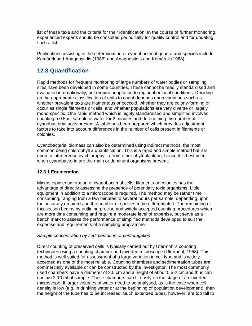
Figure 12.1 The most frequently occurring species of cyanobacteria known to produce toxins

Coelosphaerium

Gomphosphaeria

Microcystis

Synechococcus

Synechocystis

Pseudanabaena

Oscillatoria

Trichodesmium

Schizothrix

Lyngbya

Phormidium

Cylindrospermopsis

Aphanizomenon

Nostoc

Anabaena

Hormothamnion

Nodularia

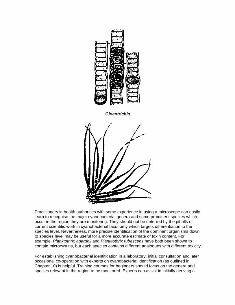
Gloeotrichia

Practitioners in health authorities with some experience in using a microscope can easily learn to recognise the major cyanobacterial genera and some prominent species which occur in the region they are monitoring. They should not be deterred by the pitfalls of current scientific work in cyanobacterial taxonomy which targets differentiation to the species level. Nevertheless, more precise identification of the dominant organisms down to species level may be useful for a more accurate estimate of toxin content. For example, Planktothrix agardhii and Planktothrix rubescens have both been shown to contain microcystins, but each species contains different analogues with different toxicity.

For establishing cyanobacterial identification in a laboratory, initial consultation and later occasional co-operation with experts on cyanobacterial identification (as outlined in Chapter 10) is helpful. Training courses for beginners should focus on the genera and species relevant in the region to be monitored. Experts can assist in initially deriving a

list of these taxa and the criteria for their identification. In the course of further monitoring, experienced experts should be consulted periodically for quality control and for updating such a list.

Publications assisting in the determination of cyanobacterial genera and species include Komárek and Anagnostidis (1986) and Anagnostidis and Komárek (1988).

12.3 Quantification

Rapid methods for frequent monitoring of large numbers of water bodies or sampling sites have been developed in some countries. These cannot be readily standardised and evaluated internationally, but require adaptation to regional or local conditions. Deciding on the appropriate classification of units to count depends upon variations such as whether prevalent taxa are filamentous or coccoid, whether they are colony-forming or occur as single filaments or cells, and whether populations are very diverse or largely mono-specific. One rapid method which is highly standardised and simplified involves counting a 0.5 ml sample of water for 2 minutes and determining the number of cyanobacterial units present. A table has been prepared which provides adjustment factors to take into account differences in the number of cells present in filaments or colonies.

Cyanobacterial biomass can also be determined using indirect methods, the most common being chlorophyll a quantification. This is a rapid and simple method but it is open to interference by chlorophyll a from other phytoplankton, hence it is best used when cyanobacteria are the main or dominant organisms present.

12.3.1 Enumeration

Microscopic enumeration of cyanobacterial cells, filaments or colonies has the advantage of directly assessing the presence of potentially toxic organisms. Little equipment in addition to a microscope is required. The method may be rather time consuming, ranging from a few minutes to several hours per sample, depending upon the accuracy required and the number of species to be differentiated. The remaining of this section begins by outlining precise and widely accepted counting procedures which are more time consuming and require a moderate level of expertise, but serve as a bench mark to assess the performance of simplified methods developed to suit the expertise and requirements of a sampling programme.

Sample concentration by sedimentation or centrifugation

Direct counting of preserved cells is typically carried out by Utermöhl's counting techniques using a counting chamber and inverted microscope (Utermöhl, 1958). This method is well suited for assessment of a large variation in cell type and is widely accepted as one of the most reliable. Counting chambers and sedimentation tubes are commercially available or can be constructed by the investigator. The most commonly used chambers have a diameter of 2.5 cm and a height of about 0.5-2 cm and thus can contain 2-10 ml of sample. These chambers can fit easily on the stage of an inverted microscope. If larger volumes of water need to be analysed, as is the case when cell density is low (e.g. in drinking water or at the beginning of population development), then the height of the tube has to be increased. Such extended tubes, however, are too tall to

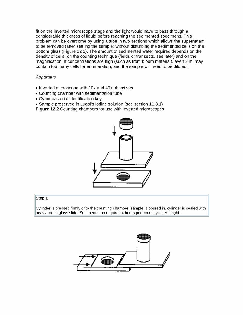
fit on the inverted microscope stage and the light would have to pass through a considerable thickness of liquid before reaching the sedimented specimens. This problem can be overcome by using a tube in two sections which allows the supernatant to be removed (after settling the sample) without disturbing the sedimented cells on the bottom glass (Figure 12.2). The amount of sedimented water required depends on the density of cells, on the counting technique (fields or transects, see later) and on the magnification. If concentrations are high (such as from bloom material), even 2 ml may contain too many cells for enumeration, and the sample will need to be diluted.

Apparatus

• Inverted microscope with 10x and 40x objectives • Counting chamber with sedimentation tube • Cyanobacterial identification key • Sample preserved in Lugol's iodine solution (see section 11.3.1) Figure 12.2 Counting chambers for use with inverted microscopes

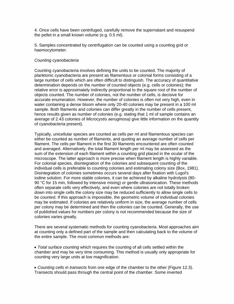
Step 1

Cylinder is pressed firmly onto the counting chamber, sample is poured in, cylinder is sealed with heavy round glass slide. Sedimentation requires 4 hours per cm of cylinder height.

Step 2

Thin, square cover slide is used to slide cylinder and supernatant off the counting chamber.

Procedure

1. Allow the sample to equilibrate to room temperature. If cold samples are placed directly in the counting chamber, air-bubbles develop and prevent sedimentation.

2. Gently invert the bottle containing the sample several time to ensure even mixing of the phytoplankton.

3. Pour the sample into the sedimentation tube in place over the counting chamber.

4. Place the counting chamber on a horizontal surface where it will not be disturbed or exposed to direct sunlight.

5. Allow the sample to settle. Sedimentation times will vary depending on the height of the sedimentation tube. Allow at least 3-4 hours per cm height of liquid. Where neutralised formalin has been used as a preservative, double the time allowed for sedimentation. Note that buoyant cells (i.e. those with gas vesicles) may not settle and may require disruption of the gas vacuoles (see below). However, this problem is frequently overcome by several days of storage with Lugol's solution, because uptake of iodine increases the specific weight of the cells.

6. Phytoplankton density can now be determined by counting either the total number of organisms on the base of the chamber or by counting subsections (transects, fields).

If an inverted microscope is not available, and samples with low cyanobacterial density need to be counted, other techniques may be applied in order to concentrate samples sufficiently (e.g. sedimentation in a measuring cylinder, followed by careful removal of the supernatant).

Apparatus

• Glass measuring cylinder, 100 ml • Glass pipette with pipette bulb or filler • Standard laboratory microscope with 10x and 40x objectives • Sample preserved in Lugol's iodine solution (section 11.3.1) Procedure 1. Allow the sample to equilibrate to room temperature.

2. Gently invert the bottle containing the sample several times to ensure even mixing of the phytoplankton.

3. Pour 100 ml of the sample into the measuring cylinder.

4. Allow the sample to sediment (3-4 hours per cm height of liquid) in a location where it will be out of direct sunlight and it will not be disturbed.

5. Using the glass pipette with pipette bulb or filler attached, carefully remove the supernatant, leaving only the last 5 ml undisturbed.

6. The sample has now been concentrated by a factor of 20 and can be counted using a counting chamber (e.g. Sedgewick-Rafter or haemocytometer).

Where sedimentation is not possible, centrifugation can offer a rapid and convenient method of concentrating a sample (Ballantine, 1953). Fixation with Lugol's iodine solution enhances the susceptibility of cells to separation by centrifugation. However, buoyant cells (i.e. those with gas vesicles) may still be difficult to pellet and may require disruption of vacuoles prior to centrifugation by applying sudden hydrostatic pressure (see below) (Walsby, 1992). Once concentrated, a known volume can be quantified using a counting chamber or by counting a defined volume using a micropipette to place a drop on a microscope slide. Observation and counting can be done with a standard microscope.

Apparatus

• Centrifuge • Centrifuge tube, 10-20 ml • Syringe or bottle with cork, or plastic bottle with screw cap • Standard laboratory microscope with 10x and 40x objectives Reagents • Aluminium potassium sulphate, 1.0 g AIK(SO4)2.12H2O in 100 ml distilled water Procedure 1. Place 10-20 ml of sample in a centrifuge tube, seal with cap, and centrifuge at 360 × g for 15 minutes.

2. When pelleting needs to be enhanced, add 0.05 ml of aluminium potassium sulphate solution per 10 ml of sample. Mix and centrifuge as described.

3. Where problems occur with the pelleting of buoyant cells, try one of the following:

i) Place sample in a plastic syringe, ensure the end is tightly sealed, then apply pressure to the plunger.

ii) Place sample in a bottle with a tightly fitting cork then bang the cork suddenly.

iii) Place sample in a well sealed plastic bottle and bring it down sharply onto a hard surface.

These three approaches should be carried out with extreme care to avoid accidental exposure to toxic cyanobacteria. Once they have been subjected to this pressure shock, the gas vesicles should have been disrupted and cells should pellet when centrifuged.

4. Once cells have been centrifuged, carefully remove the supernatant and resuspend the pellet in a small known volume (e.g. 0.5 ml).

5. Samples concentrated by centrifugation can be counted using a counting grid or haemocytometer.

Counting cyanobacteria

Counting cyanobacteria involves defining the units to be counted. The majority of planktonic cyanobacteria are present as filamentous or colonial forms consisting of a large number of cells which are often difficult to distinguish. The accuracy of quantitative determination depends on the number of counted objects (e.g. cells or colonies); the relative error is approximately indirectly proportional to the square root of the number of objects counted. The number of colonies, not the number of cells, is decisive for accurate enumeration. However, the number of colonies is often not very high, even in water containing a dense bloom where only 20-40 colonies may be present in a 100 ml sample. Both filaments and colonies can differ greatly in the number of cells present, hence results given as number of colonies (e.g. stating that 1 ml of sample contains an average of 2.43 colonies of Microcystis aeruginosa) give little information on the quantity of cyanobacteria present).

Typically, unicellular species are counted as cells per ml and filamentous species can either be counted as number of filaments, and quoting an average number of cells per filament. The cells per filament in the first 30 filaments encountered are often counted and averaged. Alternatively, the total filament length per ml may be assessed as the sum of the extension of each filament within a counting grid placed in the ocular of the microscope. The latter approach is more precise when filament length is highly variable. For colonial species, disintegration of the colonies and subsequent counting of the individual cells is preferable to counting colonies and estimating colony size (Box, 1981). Disintegration of colonies sometimes occurs several days after fixation with Lugol's iodine solution. For more stable colonies, it can be achieved by alkaline hydrolysis (80-90 °C for 15 min, followed by intensive mixing) or gentle ultrasonication. These methods often separate cells very effectively, and even where colonies are not totally broken down into single cells the colony size may be reduced sufficiently to allow single cells to be counted. If this approach is impossible, the geometric volume of individual colonies may be estimated. If colonies are relatively uniform in size, the average number of cells per colony may be determined and then the colonies can be counted. Generally, the use of published values for numbers per colony is not recommended because the size of colonies varies greatly.

There are several systematic methods for counting cyanobacteria. Most approaches aim at counting only a defined part of the sample and then calculating back to the volume of the entire sample. The most common methods are:

• Total surface counting which requires the counting of all cells settled within the chamber and may be very time consuming. This method is usually only appropriate for counting very large units at low magnification.

• Counting cells in transects from one edge of the chamber to the other (Figure 12.3). Transects should pass through the central point of the chamber. Some inverted

microscopes are equipped with special oculars so that the transect width can be adjusted as required. However, in many cases, the horizontal or vertical sides of a simple counting grid can be used to indicate the margin of the transect. Back-calculating to a millilitre of sample requires measuring the area of the transects and of the chamber bottom as well as the volume of the counting chamber.

• Counting cyanobacteria occurring in randomly selected fields ("Sichtfeld") (Figure 12.3). It is recommended that the position of the chamber to find the next field should be changed without looking through the microscope in order to prevent a bias in the selection of fields. The Sichtfeld area covered by a counting grid is usually considered as one field. However, if no counting grid is available the total spherical Sichtfeld can be considered as a single field. Back-calculating to 1 ml of sample requires registration of the number of Sichtfelds counted, measuring the area of the Sichtfeld and of the chamber bottom, as well as knowing the volume of the counting chamber.

The density of different species in one sample can vary and there can also be several orders of magnitude difference between the size of different species; hence it is necessary to select the counting method to suit the sample. Total chamber surface counting with low magnification (100x) is required for large species whereas transect or field counting with higher magnification (200x, 400x) is used for smaller or unicellular cyanobacteria. Accurate enumeration using transects or fields assumes on even distribution of cyanobacteria on the bottom of chamber surface after sedimentation. Due to inevitable convection currents, cells very rarely settle randomly on the surface of the bottom glass and are, almost always, more dense either in the middle or around the circumference of the chamber. Sometimes density also varies between opposite edges. The inaccurate estimate that arises from uneven distribution can be minimised by transect counting. Consequently, transect counting is the preferred method and counting four perpendicular diameters minimises the error. The relation of precision to counting time is very effective if about 100 counting units (cells, colonies, filaments) are settled in one transect (for simplification, see Box 12.1). Samples are best diluted or concentrated so that the number of units of the important taxa lies within this range.

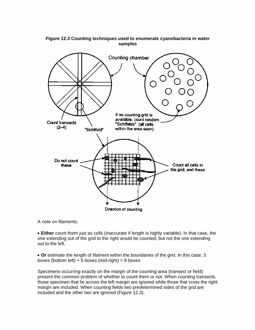
Figure 12.3 Counting techniques used to enumerate cyanobacteria in water samples

A note on filaments:

• Either count them just as cells (inaccurate if length is highly variable). In that case, the one extending out of the grid to the right would be counted, but not the one extending out to the left.

• Or estimate the length of filament within the boundaries of the grid. In this case: 3 boxes (bottom left) + 5 boxes (mid-right) = 8 boxes

Specimens occurring exactly on the margin of the counting area (transect or field) present the common problem of whether to count them or not. When counting transects, those specimen that lie across the left margin are ignored while those that cross the right margin are included. When counting fields two predetermined sides of the grid are included and the other two are ignored (Figure 12.3).

Box 12.1 Simplification for biomass estimates

With some experience and a flexible approach, the time needed for enumeration and measurement of cell dimensions can be considerably reduced (down to 1 hour or less, if only one or two species require counting) without substantial loss of accuracy. The procedure is as follows:

• If the deviation of numbers of dominant species counted in two perpendicular transects is less than 20 per cent between both transects, do not count further transects.

• If the standard deviation of cell dimensions measured on 10 cells is less than 20 per cent, do not measure further cells.

• If a set of samples from the same water body and only slightly differing sites (e.g. vertical or horizontal profiles) is to be analysed, enumerate all samples, but measure cell dimensions only from one. Check others by visual estimate for deviations of cell dimensions and conduct measurements only if deviations are suspected.

There are different recommendations regarding the number of units per species that must be counted to obtain reliable data. It is particularly difficult to count each species with an acceptable error (20-30 per cent if 400 individual units are counted) in each sample. Mass developments of cyanobacteria are characterised by dominance of one to three species. Even if total phytoplankton is to be counted (for example in order to assess the relative share of cyanobacteria), it is rare for more than six to eight species to contribute to the majority of the biomass. Therefore, for total phytoplankton counts, it is suggested that 400-800 specimens in each sample are counted, giving a maximum error for the total count as 7-10 per cent. In this situation there will be a 10-20 per cent error for the few dominant species, 20-60 per cent for the subdominant species and the rest of the species can be considered as insufficiently counted. If only cyanobacteria are to be counted, and only one or two species are present, counting up to the precision level of 20 per cent, by counting 400 individual units per species, can be accomplished within less than one hour.

The use of mechanical or electronic counters for recording cell counts can shorten counting time considerably, especially if only a few species are counted. Computer keyboards can also be used together with suitable programmes for recording cell counts.

The use of an inverted microscope with counting chambers is generally the best approach for estimating cyanobacterial numbers. However, a standard microscope is sufficient for preconcentrated samples or for naturally dense samples from mass developments, provided the size of the water drop enumerated can be defined (e.g. by using a micropipette). Other counting chambers (e.g. Sedgewick-Rafter or haemocytometer) are available for use with a standard microscope. It can also be useful to monitor samples under high magnification with oil-immersion (1,000x) to check the sample for the presence of very small species which may be overlooked during normal counting.

An alternative counting method which has been found to be useful is syringe filtration. This method is considerably less time consuming because it does not depend on lengthy sedimentation times and uses a standard laboratory microscope.

Apparatus

• Syringe, 10 ml • Membrane filters, 13 mm diameter with 0.45 µm pore • Membrane filter holder • Glass microscope slides plus coverslips • Standard laboratory microscope with 10x and 40x objectives Reagents • Immersion oil Procedure 1. Mix water sample by inverting several times.

2. Take up 10 ml of the sample into the syringe.

3. Place filter holder with filter in place, on the end of the syringe.

4. Gently filter the sample through the filter by applying pressure to the syringe piston.

5. Once all the sample has passed through the filter, remove the filter from the holder and place it on a glass microscope slide with the captured cells uppermost.

6. Allow the filter to dry at room temperature then carefully add one or two drops of immersion oil to the filter. The will make the filter appear transparent and permit observation of the cyanobacterial cells trapped on its surface.

7. Finally, cover the filter surface with a glass coverslip and examine under the microscope.

8. The density of cyanobacteria can be easily calculated by counting the number of cells on the filter and dividing this by the volume of water filtered (i.e. number of cells per ml).

12.3.2 Determination of cyanobacterial biomass microscopically

Cell size can vary considerably within and between species, and toxin concentration relates more closely to the amount of dry matter in a sample than to the number of cells. Hence, cell numbers are often not an ideal measure of population size or potential toxicity. This can be overcome by determining biomass. Two approaches are available, either estimation from cell counts and average cell volumes, or from chemical analysis of pigment content.

Cyanobacterial counts and cell volumes

Biovolume can be obtained from cell counts by determining the average cell volume for each species or unit counted and then multiplying this value by the cell number present in the sample. The result is the total volume of each species. Given a specific weight of almost 1 mg mm-3 for plankton cells, this biovolume corresponds quite closely to biomass. Average volumes are determined by assuming idealised geometric bodies for each species (e.g. spheres for Microcystis cells, cylinders for filaments), measuring the relevant geometric dimensions of 10 to 30 cells (depending upon variability) of each

species, and calculating the corresponding mean volume of the respective geometric body.

Example 1

By measuring 20 Microcystis cells, an average diameter of 5 µm was established. Assuming spherical-shaped cells the average cell volume is 4/3 πr3 = 65.4 µm3. Enumeration resulted in 1 million cells per ml and thus the total biovolume is 65.4 × 106 µm3 ml-1.

Example 2

Measuring 30 Planktothrix filaments resulted in an average length of 225 µm and an average diameter of 6 µm. Assuming cylindrical shaped filaments, the average filament volume is 2 πr2 × L = 6,359 µm3. Enumeration resulted in 10,000 filaments per ml. Thus the biovolume of Planktothrix was 63.6 × 106 µm3 ml-1.

Thus, although the number of Planktothrix was 100-fold less than that of Microcystis, biovolumes were similar because the volume (and biomass) of a single Planktothrix filament is about 100 times as large as that of a single Microcystis cell. Both species often contain microcystins, and it is possible to compare the relative toxin content per biovolume or biomass whereas there is little point in comparing toxin content in relation to the respective cell numbers.

12.4 Determination of biomass using chlorophyll a analysis

The pigment chlorophyll a generally contributes 0.5-1 per cent of the ash-free dry weight of phytoplankton organisms. Although the pigment content may vary according to the physiological state of the organisms (e.g. it increases if light availability is low), chlorophyll a is a widely used and accepted measure of biomass. It is an especially useful measure during cyanobacterial blooms, when the phytoplankton chiefly consists of cyanobacteria, often of only one species. However, when chlorophyll a determination is used with mixed phytoplankton populations (cyanobacteria and other species), it gives an overestimation of cyanobacterial biomass. Rough microscopic estimations of the relative share of cyanobacterial cells among the total phytoplankton may be used to correct the overestimate.

Analysis of chlorophyll a requires relatively simple laboratory equipment, principally filtration apparatus, centrifuge and spectrophotometer. It is considerably less time-consuming than microscopic biomass determination (but also less specific and less precise). Standard protocols have been described (e.g. ISO, 1992) but preferred methods vary somewhat between laboratories. However, the main procedural steps in most methods are essentially the same: solvent extraction of chlorophyll a, determination of the concentration of the pigment by spectrophotometry, and adjustments to the result to reduce the interference by phaeophytin a which is a degradation product of chlorophyll a. A simple method following the ISO procedure for the determination of chlorophyll a in a lake water sample is outlined below.

Apparatus

• Spectrophotometer suitable for readings up to 750 nm, or photometer with discrete wavelengths at 665 and 750 nm

• Glass cuvettes, typically of 1 cm path length, or 5 cm for very low concentrations (e.g. from drinking water reservoirs at the beginning of population development)

• Centrifuge

• 15 ml centrifuge tubes, graduated and with screw caps

• Water bath at 75 °C or other heating device for boiling ethanol

• Glass fibre filters (GF/C), 47 mm diameter

• Filtration apparatus and vacuum pump

• Tissue grinder or ultrasonication device

• Pipette or similar for addition of acid

Reagents • Ethanol (90 % aqueous) • Hydrochloric acid, 1 mol l-1 Procedure

Perform the following steps in low intensity of indirect light because light induces rapid degradation of chlorophyll.

1. After recording the initial volume of water, separate the cells from the water by filtration. Filter continuously and do not allow the filter to dry during filtration of a single sample. If extraction cannot be performed immediately, filters should be placed in individual, labelled bags (filters folded in half with cells innermost) or Petri dishes and stored at -20 °C in the dark (this may cause some pigment degradation and is not recommended by ISO). This step can be carried out at the sampling site and the samples are readily transported in this form. In preference to freezing, samples may be stored in the extraction medium (see below) for up to 4 days in the refrigerator.

2. Place the filter in a tissue grinder, add 2-3 ml of boiling ethanol, and grind until the filter fibres are separated. Ultrasonication can also be used. Pour the ethanol and ground filter into a centrifuge tube, rinse out the grinding tube with another 2 ml ethanol and add this to the centrifuge tube. Make up to a total of 10 ml in the centrifuge tube with ethanol. Place cap on the tube, label and store in darkness at approximately 20 °C for 24-48 hours.

3. Centrifuge for 15 minutes at 3,000-5,000 g to clarify samples. Decant the clear supernatant into a clean vessel and record the volume.

4. Blank Spectrophotometer with 90 per cent ethanol solution at each wavelength.

5. Place centrifuged sample in the cuvette and record absorbance at 750 nm and 665 nm (750a and 665a; absorbance at 750 is for turbidity correction and should be very low). Readings at 665 nm should range between 0.1 and 0.8 units.

6. Add 0.01 ml of 1 mol I-1 HCl to sample in cuvette (adjust volume to suit the volume of cuvette being used, calculating approximately 0.003 ml of 1 mol l-1 HCl per ml of ethanol solution) and agitate gently for 1 minute. Record absorbance at 750 nm and 665 nm (750b and 665b).

Calculation 1. Correct for turbidity by subtracting absorbance 665a-750a = corrected 665a absorbance 665b-750b = corrected 665b absorbance 2. Use the corrected 665a and 665b absorbance to calculate:

where: Ve = Volume of ethanol extract (ml) Vs = Volume of water sample (litres) l = Path length of cuvette (cm) Note, the ratio of chlorophyll a to phaeophytin a should give an indication of the condition of the cyanobacterial (and algal) population, but may also reflect the effectiveness of sample handling and preservation, because high levels of phaeophytin a indicate degradation of chlorophyll a either in scenescent field populations or during analysis. When samples are concentrated by filtration for the purposes of analysis, the cells die. Consequently, the chlorophyll immediately starts to degrade to phaeopigments. If filters are not rapidly extracted or frozen, chlorophyll a concentrations are thus reduced. Occasionally, other factors affect this method, resulting in very low or even negative values for chlorophyll a. This can be checked by calculating:

The result of this calculation should give a similar value to the sum of the concentrations of both pigments determined separately, as above. Note also:

• If no centrifuge is available, filtration may be used instead.

• If no tissue grinder or ultrasonication device is available, proceed without this step. Slight underestimations may occur. For cyanobacteria, these are not likely to be too serious.

12.5 Determination of nutrient concentrations

The capacity for development of a cyanobacterial bloom depends on the available concentrations of elements that the cells are composed of (chiefly carbon, hydrogen, oxygen, phosphorus, nitrogen and sulphur). These elements are needed in the ratio in which they occur in living cells (in weight units: 42 C, 8.5 H, 57 O, 7 N, 1 P and 0.7 S). Hydrogen and oxygen are available in unlimited supply in an aqueous environment, and sulphur is usually also present in surplus concentrations. Carbon has been investigated as a potentially limiting factor, but has rarely been found to be relevant. Most often, phosphorus concentrations limit the amount of biomass that can form in a given water body but sometimes, nitrogen is limiting. The chief sources of nitrogen are nitrate and ammonia, but to some extent their lack can be compensated by some cyanobacteria through fixation of atmospheric nitrogen. Thus, even if phosphate is clearly the factor limiting carrying capacity, knowledge of nitrogen availability helps to predict whether nitrogen-fixing species are likely to grow.

Cyanobacterial cells appear to have little means of storing excess nitrogen, but can store enough phosphate for up to four cell divisions, which implies that one cell can grow into 16 without needing to take up dissolved phosphate. Information on dissolved phosphate concentrations, therefore, only demonstrates that if it can be detected, the phytoplankton population is not currently limited by phosphate. In order to assess the capacity of the water body to carry a cyanobacterial population, total phosphate must be determined, which can then be compared with the total concentration of nitrogen salts and organic nitrogen. However, in order to assess whether nitrogen may be limiting, analysis of dissolved components (chiefly nitrate and ammonia) is sufficient.

Among the methods available, the procedure of Koroleff (1983) for determining total phosphate has proved to be most reliable and is the basis of an ISO protocol. For nitrate and ammonia, several methods are available, but the ISO method with the least demands on equipment is described below. Details of ISO methods can be obtained directly from ISO at Case Postale 56, CH-1211, Geneva 20, or requested through the Internet on central@iso.ch.

12.5.1 Analysis of phosphorus according to ISO 6878

Phosphorus in various types of waters can be determined spectrometrically by digestion of organic phosphorus compounds to orthophosphate and reaction under acidic conditions to an antimony-phosphormolybdate complex which is then reduced to a strongly coloured blue molybdenum complex. The internationally harmonised method described by ISO/FDIS 6878 (ISO, 1998a) is applicable to many types of waters (surface-, ground-, sea- and wastewater) in a concentration range of 0.005 to 0.8 mg l-1 (or higher if samples are diluted). Differentiation by the following fractions is possible through filtration procedures:

Option Fraction Filtration/procedure 1 Soluble reactive phosphorus (SRP or orthophosphate) Filtered sample 2 Dissolved organic phosphate Digested filtered sample 3 Particulate phosphorus Option 4 minus option 2

4 Total phosphorus Digested unfiltered sample

Digestion or mineralisation of organophosphorus compounds to orthophosphate is performed in tightly sealed screw-cap vessels with persulphate, under pressure and heat in an autoclave (in the absence of which good results have also been obtained with household pressure cookers), or simply by gentle boiling. Polyphosphates and some organophosphorus compounds may also be hydrolysed with sulphuric acid to molybdate-reactive orthophosphate. The following gives an overview of the procedure, necessary equipment and chemicals, see ISO (1998) for details and specific problems.

Apparatus

• Photometer measuring absorbance in the visible and near infrared spectrum above 700 nm; sensitivity is optimal at 880 nm (and reduced by 30 per cent at 700 nm); sensitivity is increased if optical cells of 50 mm are used (if 100 mm cells are available, determination down to 0.001 mg I-1 may be possible)

• Filter assembly and membrane filters, 45 mm diameter with 0.45 µm pore

• For digestion of samples, an autoclave (or pressure cooker) suitable for 115-120 °C

• For digestion of samples, borosilicate vessels with heat-resistant caps that can be tightly sealed

• Bottles for samples as described in Chapter 11

• Pre-cleaned glass bottles for filtered samples

Reagents

All reagents should be of a recognised analytical grade and the distilled water used must have a negligible phosphorus concentration when compared with the samples

• Sulphuric acid (H2SO4): 9 mol l-1

• Sulphuric acid (H2SO4): 4.5 mol l-1

• Sulphuric acid (H2SO4): 2 mol l-1

• Sodium hydroxide (NaOH): 2 mol l-1

• Ascorbic acid (C6H8O6): 100 g l-1 (stable for 2 weeks in amber glass bottle, refrigerated)

• Acid molybdate solution I: ammonium heptamolybdate tetrahydrate [(NH4)6Mo7O24. 4 H2O] 13 g per 100 ml and antimony potassium tartrate hemihydrate [K(SbO)C4H4O6. ½ H2O] 0.35 g per 100 ml (stable for 2 months in amber glass bottle)

• Orthophosphate standard stock solution: sodium thiosulphate pentahydrate (Na2S2O3. 5H2O) 1.2 g in 100 ml water, stabilised with 0.05 g of anhydrous sodium carbonate (Na2CO3) as preservative

• Potassium peroxodisulphate: (K2S2O8) 5 g per 100 ml (stable for 2 weeks in amber glass borosilicate bottle)

Procedure

All glassware (including sampling bottles) must be washed with hydrochloric acid (1.12 g ml-1) at 40-50 °C and thoroughly rinsed. Do not use detergents containing phosphates and preferably use the glassware only for the determination of phosphorus.

For measuring orthophosphate:

1. Filter samples with pre-washed filters; discard the first 10 ml of filtrate, collect 5-40 ml (depending on concentrations expected).

2. Carry out a blank test with distilled water, using all of the reagents and performing the same procedure as for the samples.

3. Prepare orthophosphate calibration solutions in the concentration range of the samples (e.g. from 0.05 to 0.5 mg l-1) with a volumetric pipette in 50 ml volumetric flasks (filling them only up to about 40 ml).

4. Transfer samples into 50 ml volumetric flasks with volumetric pipettes. Depending on expected concentrations, use 5-40 ml of sample, fill up to about 40 ml with distilled water.

5. Add, while swirling, first 1 ml ascorbic acid solution and then 2 ml acid molybdate solution, fill flask up to the 50 ml mark with distilled water and mix well.

6. After 10-30 minutes, measure absorbance at 880 nm using distilled water in the reference cell.

7. Plot absorbance of calibration solutions against their concentration and determine slope; check for linearity. Run an independently-prepared calibration solution with each series of samples, but especially when new batches of reagents are used.

8. Occasionally dean the glassware used for developing the colour complex with sodium hydroxide solution to remove colour deposits.

For measuring total, particulate and dissolved organic phosphorus: 1. Clean digestion vessels with about 50 ml of water and 2 ml of sulphuric acid (1.84 g ml-1) in autoclave for 30 minutes at 115-120 °C, cool and rinse, repeat procedure several times, store covered.

2. Carry out a blank test with distilled water, using all of the reagents and performing the same procedure as for the samples.

3. Add 1 ml of sulphuric acid (4.5 mol l-1) to 100 ml of sample to adjust pH to about 1 (further adjustment with sulphuric acid or sodium hydroxide solution (2 mol l-1).

4. Pipette 5-40 ml of sample into digestion vessel, add 4 ml of potassium peroxodisulphate solution, mineralise in autoclave (or pressure cooker), or boil gently for 30 minutes.

5. Cool, adjust pH to between 3 and 10 with sodium hydroxide solution or sulphuric acid (2 mol l-1), transfer to 50 ml flask and proceed as above for orthophosphate.

If large quantities of organic matter are present, oxidation with nitric acid-sulphuric acid may be necessary. Furthermore, arsenate may cause interference (see ISO, 1998a).

The test report should contain complete sample identification, reference to the method used, the results obtained and any further details likely to have influence on the results.

12.5.2 Analysis of nitrate

Several methods for determination of nitrate have been provided by the ISO, the simplest being a spectrometric measurement of the yellow compound formed by reaction of sulphosalicylic acid with nitrate and subsequent treatment with alkali (ISO, 1988). The equipment required is a spectrometer operating at a wavelength of 415 nm and optical path length of 40-50 mm, evaporating dishes, a water bath capable of accepting six or more dishes, and a water bath capable of thermostatic regulation to 25 °C. This method is suitable for surface and potable water samples and has a detection limit of 0.003 to 0.013 mg l-1 (depending on optical equipment). Interference from a range of substances, particularly chloride, orthophosphate, magnesium and manganese (III) is possible. Interference problems can be avoided with other spectrometric methods ISO (1986a,b).

12.5.3 Analysis of ammonia

A manual spectrometric method is given by ISO (1984a) which analyses a blue compound formed by the reaction of ammonium with salicylate and hypochlorite ions in the presence of sodium nitrosopentacyanoferrate (III) at a limit of detection of 0.003-0.008 mg l-1. An automated procedure is given by ISO (1986c). A distillation and titration method is given by ISO (1984b).

12.6 References

Anagnostidis, K. and Komárek, J. 1988 Modern approach to the classification system of cyanophytes. Archiv Hydrobiol., Supplement 80, Algological Studies, 50-53, 327-472.

Ballantine, D. 1953 Comparison of different methods of estimating nanoplankton. J. Mar. Biol. Ass. UK, 32, 129-147.

Box J.D. 1981 Enumeration of cell concentrations in suspensions of colonial freshwater microalgae, with particular reference to Microcystis aeruginosa. Brit. Phycol. J., 16, 153-164.

ISO 1984a Water Quality - Determination of Ammonium - Part 1: Manual spectrometric method. ISO 7150-1, International Organization for Standardization, Geneva.

ISO 1984b Water Quality - Determination of Ammonium - Distillation and titration method. ISO 5664, International Organization for Standardization, Geneva.

ISO 1986a Water Quality - Determination of Nitrate - Part 1: 2,6-Dimethylphenol spectrometric method. ISO 7890-1, International Organization for Standardization, Geneva.

ISO 1986b Water Quality - Determination of Nitrate - Part 2: 4-Fluorophenol spectrometric method after distillation. ISO 7890-2, International Organization for Standardization, Geneva.

ISO 1986c Water Quality - Determination of Ammonium - Part 2: Automated spectrometric method. ISO 7150-2, International Organization for Standardization, Geneva.

ISO 1988 Water Quality - Determination of Nitrate - Part 3: Spectrometric method using sulfosalicylic acid. ISO 7890-3, International Organization for Standardization, Geneva.

ISO 1998a Water Quality - Spectrometric determination of phosphorus using ammonium molybdate. ISO/FDIS 6878, International Organization for Standardization, Geneva.

ISO 1992 Water Quality - Measurement of biochemical parameters. Spectrometric determination of the chlorophyll-a concentrations. ISO 10260, International Organization for Standardization, Geneva.

Komárek, J. and Anagnostidis, K. 1986 Modern approach to the classification system of cyanophytes. Archiv Hydrobiol., Supplement 73, Algological Studies, 43, 157-164.

Koroleff, F. 1983 Determination of phosphorus. In: K. Grasshoff, M. Ehrhardt and K. Kremling [Eds] Methods of Seawater Analysis. Verlag Chemie, Weinheim, Deerfield Beach, FL, Basel, 125-139.

Utermöhl, H. 1958 Zur Vervollkommnung der quantitative Phytoplankton-Methodik. Mitt. int. Verein. theor. angew. Limnol. 5, 567-596.

Walsby, A.E. 1992 The control of gas-vacuolated Cyanobacteria. In: D.W. Sutcliffe and G. Jones [Eds] Eutrophication: Research and Application to Water Supply. Freshwater Biological Association, Windermere, 143-162.