Prof. David R. Jackson Dept. of ECE

Fall 2016

Notes 4

ECE 6340 Intermediate EM Waves

1

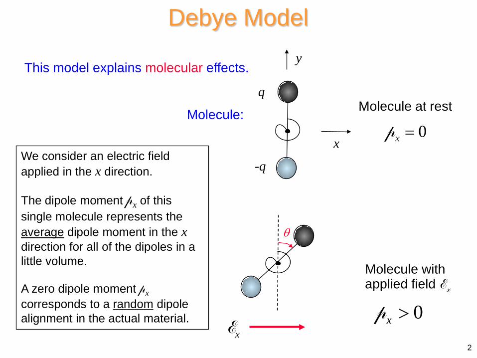
Debye Model

Molecule:

This model explains molecular effects.

Molecule at rest

Molecule with applied field Ex

0x =p

0>xp

We consider an electric field applied in the x direction. The dipole moment px of this single molecule represents the average dipole moment in the x direction for all of the dipoles in a little volume. A zero dipole moment px corresponds to a random dipole alignment in the actual material.

q

-q

x

y

xE

θ

2

3

Debye Model (cont.)

xE

θ

x

y Torque on dipole due to electric field:

( ) ( )( )

ET r q r q

r r q

p

+ −

+ −

= × + × −

= − ×

= ×

E E

E

E

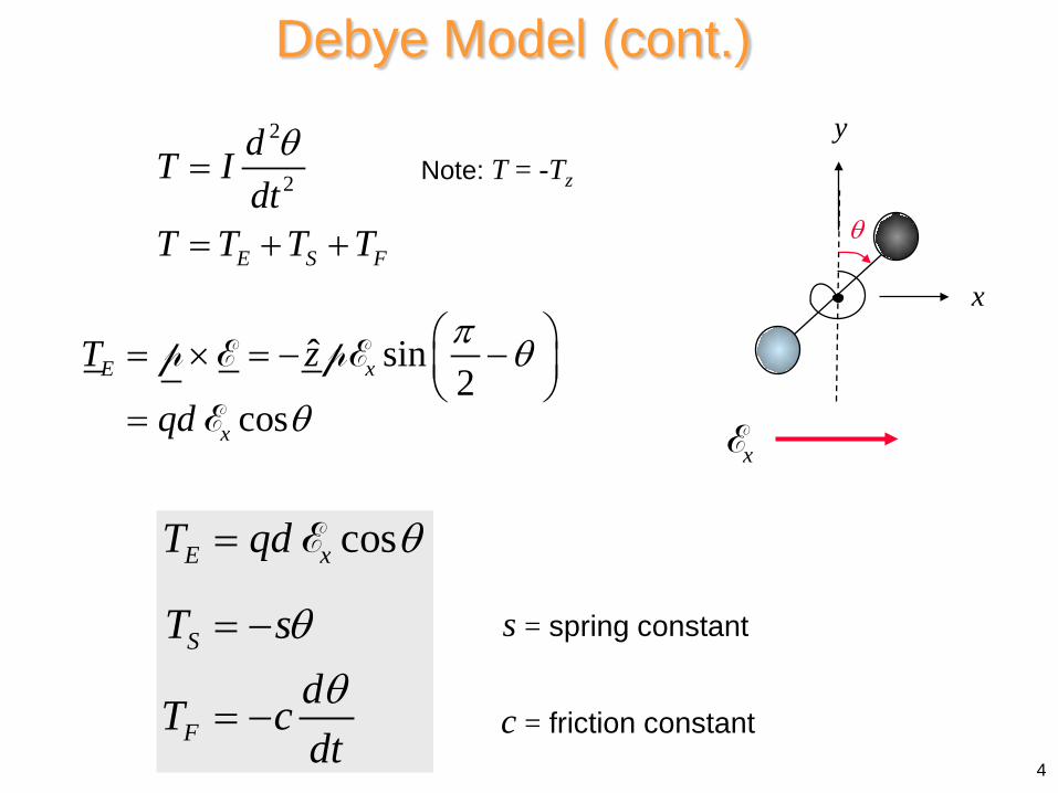
Debye Model (cont.) 2

2

E S F

dT Idt

T T T T

θ=

= + +

cosE x

S

F

T qd

T sdT cdt

θ

θθ

=

= −

= −

E

s = spring constant

c = friction constant

Note: T = -Tz

ˆ sin2

cosE x

x

T z

qd

π θ

θ

= × = − −

=

p E pE

E

4

xE

θ

x

y

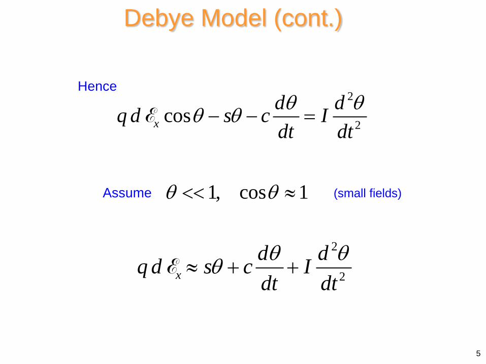
Hence

Assume

2

2cosxd dq d s c Idt dtθ θθ θ− − =E

1, cos 1θ θ<< ≈

2

2xd dq d s c Idt dtθ θθ≈ + +E

Debye Model (cont.)

5

(small fields)

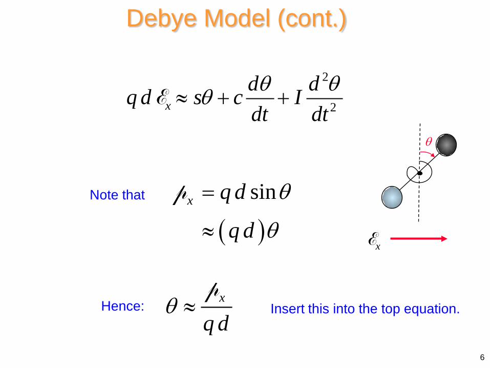
( )sinx q d

q d

θ

θ

=

≈

pNote that

2

2xd dq d s c Idt dtθ θθ≈ + +E

Hence: θ ≈ x

q dp

Insert this into the top equation.

Debye Model (cont.)

6

xE

θ

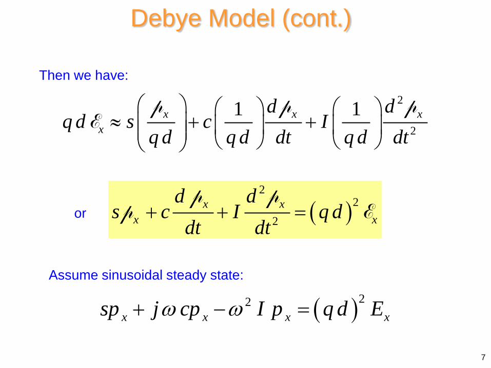
Then we have:

Assume sinusoidal steady state:

or

2

2

1 1x x xx

d dq d s c I

q d q d dt q d dt

≈ + +

p p pE

( )2

22

x xx x

d ds c I q d

dt dt+ + =

p pp E

( )22x x x xsp j cp I p q d Eω ω+ − =

Debye Model (cont.)

7

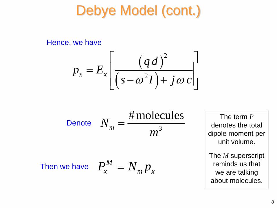
Hence, we have

Then we have

( )( )

2

2x x

q dp E

s I j cω ω

=

− +

3

#moleculesmN

m=

Mx m xP N p=

The term P denotes the total

dipole moment per unit volume.

The M superscript reminds us that we are talking

about molecules.

Debye Model (cont.)

Denote

8

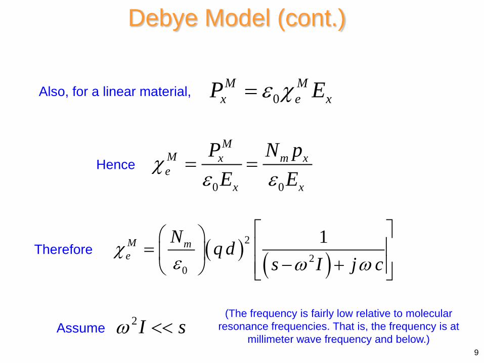
Also, for a linear material,

Hence

0M M

x e xP Eε χ=

0 0

MM x m xe

x x

P N pE E

χε ε

= =

Therefore ( ) ( )2

20

1M me

N q ds I j c

χε ω ω

=

− +

Assume 2I sω <<(The frequency is fairly low relative to molecular

resonance frequencies. That is, the frequency is at millimeter wave frequency and below.)

Debye Model (cont.)

9

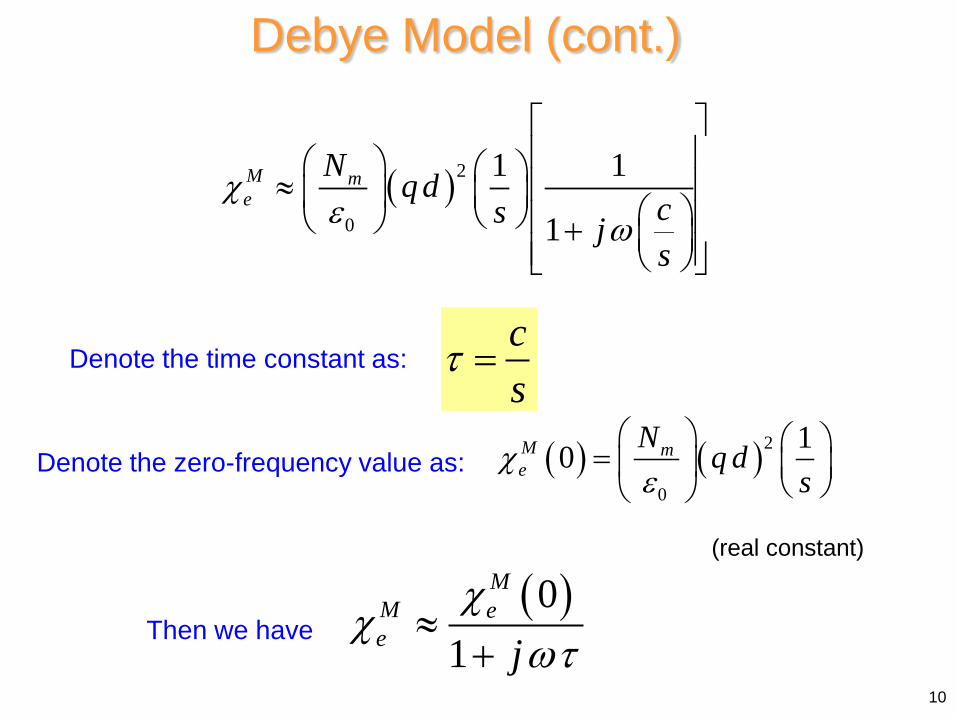
Denote the time constant as:

( )2

0

1 1

1

M me

N q dcs js

χε ω

≈ +

cs

τ =

( ) ( )2

0

10M me

N q ds

χε

=

( )01

MM ee j

χχ

ωτ≈

+

Denote the zero-frequency value as:

Debye Model (cont.)

(real constant)

Then we have

10

( )01

MM ee j

χχ

ωτ≈

+

Debye Model (cont.)

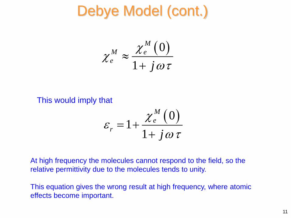
This would imply that

( )01

1

Me

r jχ

εωτ

= ++

At high frequency the molecules cannot respond to the field, so the relative permittivity due to the molecules tends to unity. This equation gives the wrong result at high frequency, where atomic effects become important.

11

( )01

MeM

e jχ

χωτ

=+

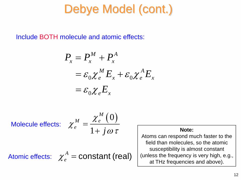
Include BOTH molecule and atomic effects:

Debye Model (cont.)

Molecule effects:

Atomic effects:

0 0

0

M Ax x x

M Ae x e x

e x

P P PE E

Eε χ ε χε χ

= +

= +

=

Aeχ = constant (real)

Note: Atoms can respond much faster to the

field than molecules, so the atomic susceptibility is almost constant

(unless the frequency is very high, e.g., at THz frequencies and above).

12

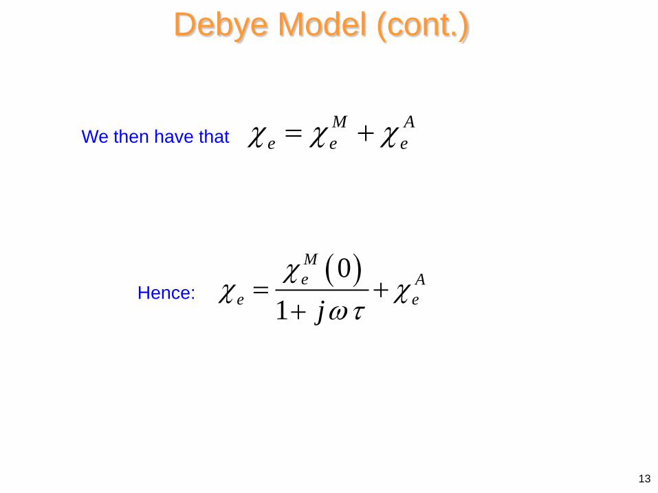
We then have that M A

e e eχ χ χ= +

( )01

Me A

e ejχ

χ χωτ

= ++

Debye Model (cont.)

Hence:

13

Permittivity formula: 1r eε χ= +

( )

21

01

1

1

MeA

r e jaaj

χε χ

ωτ

ωτ

= + ++

= ++

( )1

2

1

0

Ae

Me

aa

χ

χ

= +

=

where

Debye Model (cont.)

(a1 and a2 are real constants.)

14

Hence, we have

( )( )

1 2

1

0r

r

a a

a

ε

ε

= +

∞ =

so ( )( ) ( )

1

2 0r

r r

a

a

ε

ε ε

= ∞

= − ∞

( ) ( ) ( )01

r rr r j

ε εε ε

ωτ− ∞

= ∞ ++

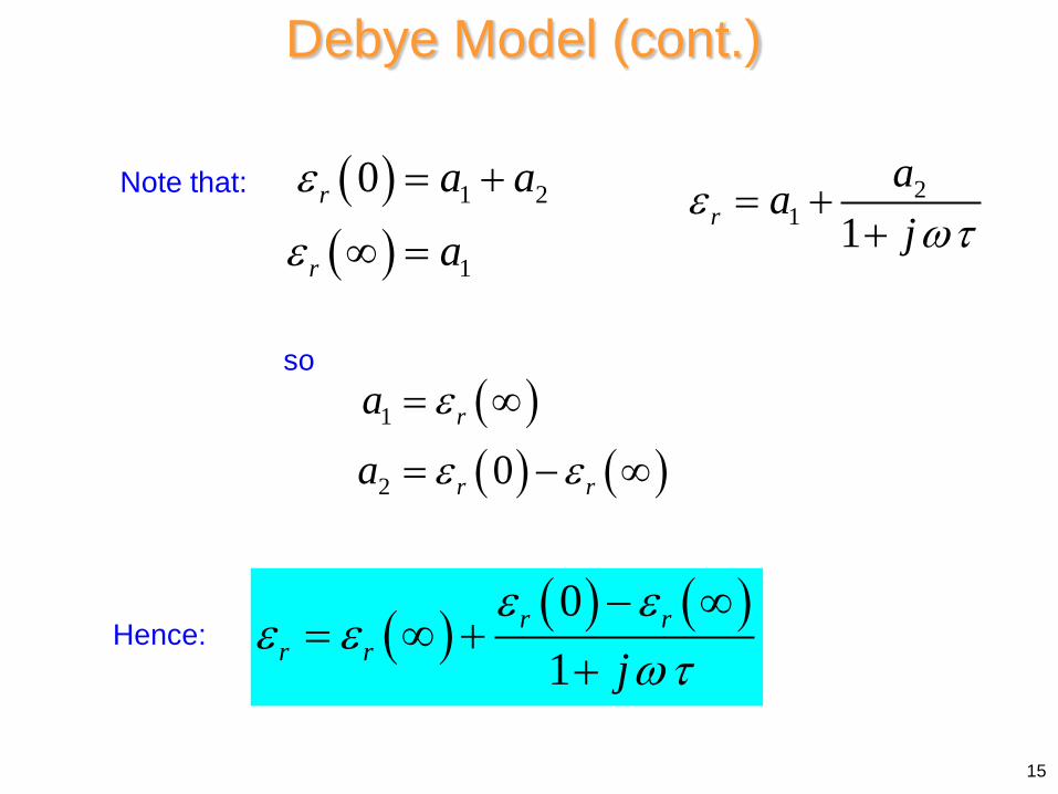
Note that:

Hence:

Debye Model (cont.)

21 1r

aaj

εωτ

= ++

15

( ) ( ) ( )( )

( ) ( )( )

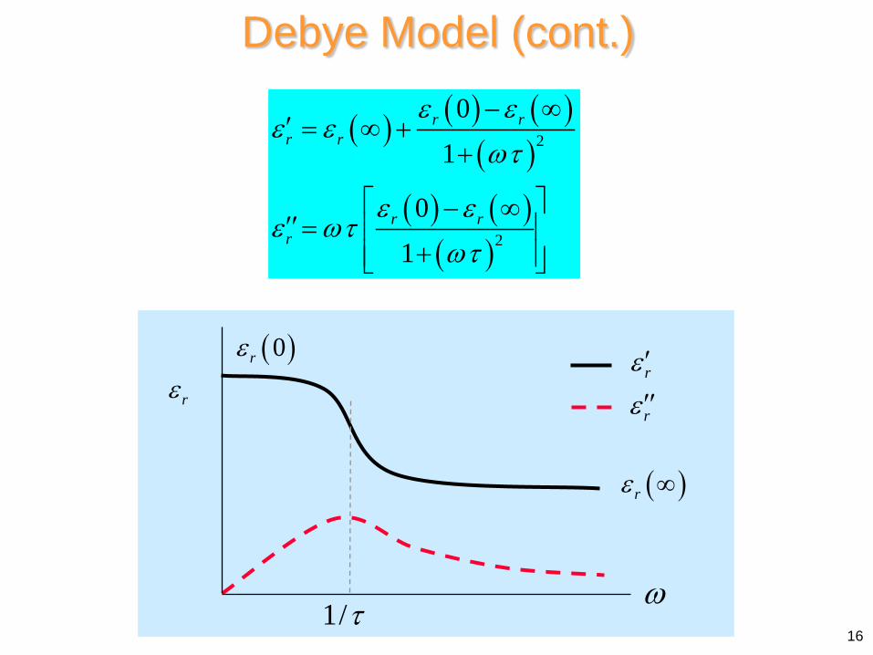
2

2

01

01

r rr r

r rr

ε εε ε

ωτ

ε εε ωτ

ωτ

− ∞′ = ∞ +

+

− ∞′′=

+

( )rε ∞

( )0rε

rε

1/τ

rε ′

rε ′′

ω

Debye Model (cont.)

16

Frequency for maximum loss:

Let x ωτ=

( ) ( )( )2 01r r r

xx

ε ε ε ′′= − ∞ +

A maximum occurs at 1x =

1ωτ

=or

Debye Model (cont.)

17

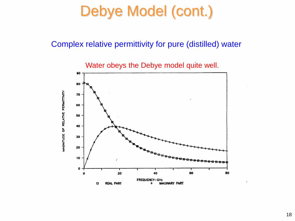
Water obeys the Debye model quite well.

18

Water obeys the Debye model quite well.

Debye Model (cont.)

Complex relative permittivity for pure (distilled) water

Water obeys the Debye model quite well.

19

Ocean water: σ = 4 [S/m]

Example

Calculate the complex relative permittivity εrc for ocean water at 10.0 GHz.

0 0 0

1crc rj jε σ σε ε ε

ε ε ω ωε = = − = −

( ) ( )( )9 12

460 352 10.0 10 8.854 10rc j jεπ −

= − −× ×

from previous plot for distilled water

60 42.19rc jε = −( ) ( )60 35 7.19rc j jε = − −Hence

or

Cole-Cole Model

This is a modification of the Debye model.

( ) ( ) ( )( )1

01

r rr r j α

ε εε ε

ωτ −

− ∞= ∞ +

+

When α = 0, the model reduces to the Debye model.

This model has often been used to describe the permittivity of some polymers, as well as biological tissues.

20

Cole-Cole Model (Cont.) Parameters for Some Biological Tissues

21

Havriliak–Negami Model

This is another modification of the Debye model.

( ) ( ) ( )( )( )0

1

r rr r

jβα

ε εε ε

ωτ

− ∞= ∞ +

+

When α = 1 and β = 1, the model reduces to the Debye model.

This has been used to describe the permittivity of some polymers.

22

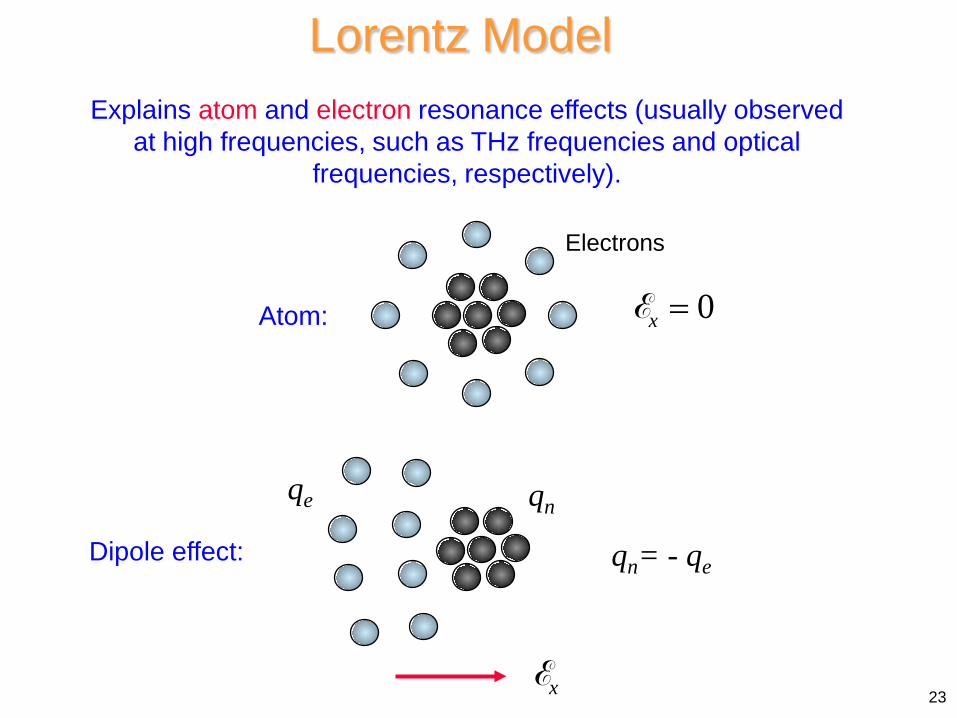
Lorentz Model Explains atom and electron resonance effects (usually observed

at high frequencies, such as THz frequencies and optical frequencies, respectively).

Dipole effect:

Atom:

xE

qn= - qe

qn qe

0=xE

Electrons

23

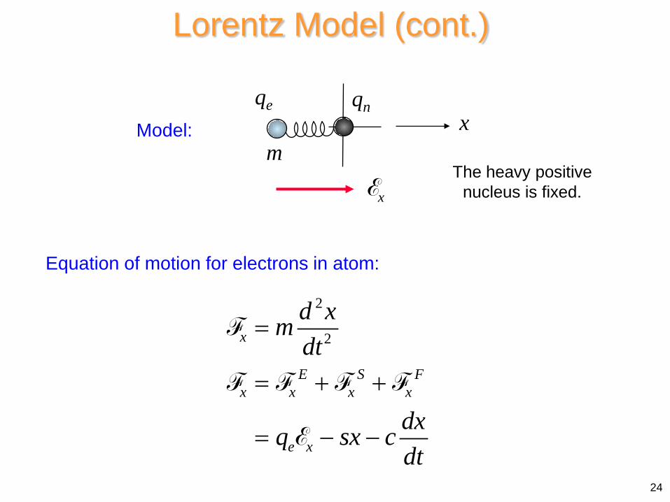
Lorentz Model (cont.)

Model:

Equation of motion for electrons in atom:

x

qn qe

m

xE

2

2x

E S Fx x x x

e x

d xmdt

dxq sx cdt

=

= + +

= − −

F

F F F F

E

The heavy positive nucleus is fixed.

24

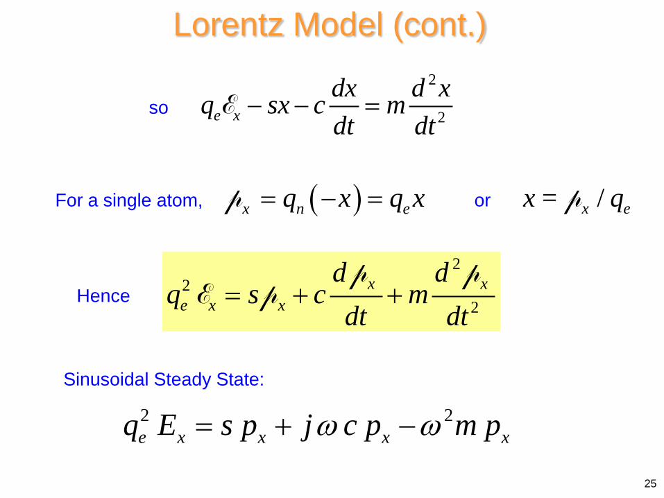
so

Hence

2

2e xdx d xq sx c mdt dt

− − =E

( )x n eq x q x= − =p

22

2= + +x xe x x

d dq s c m

dt dtp p

E p

Sinusoidal Steady State:

2 2e x x x xq E s p j c p m pω ω= + −

For a single atom, = /x ex qpor

Lorentz Model (cont.)

25

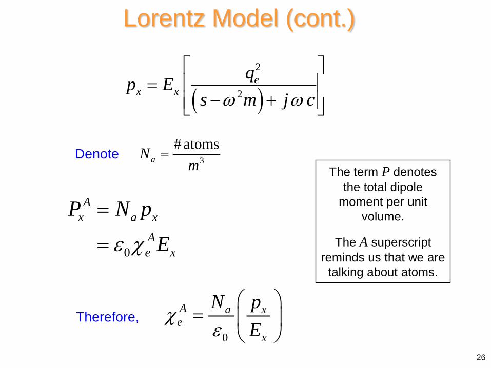
Therefore,

( )2

2e

x xqp E

s m j cω ω

=

− +

0

Ax a x

Ae x

P N pEε χ

=

=

0

A a xe

x

N pE

χε

=

The term P denotes the total dipole

moment per unit volume.

The A superscript reminds us that we are

talking about atoms.

Lorentz Model (cont.)

26

3

#atomsaN

m=Denote

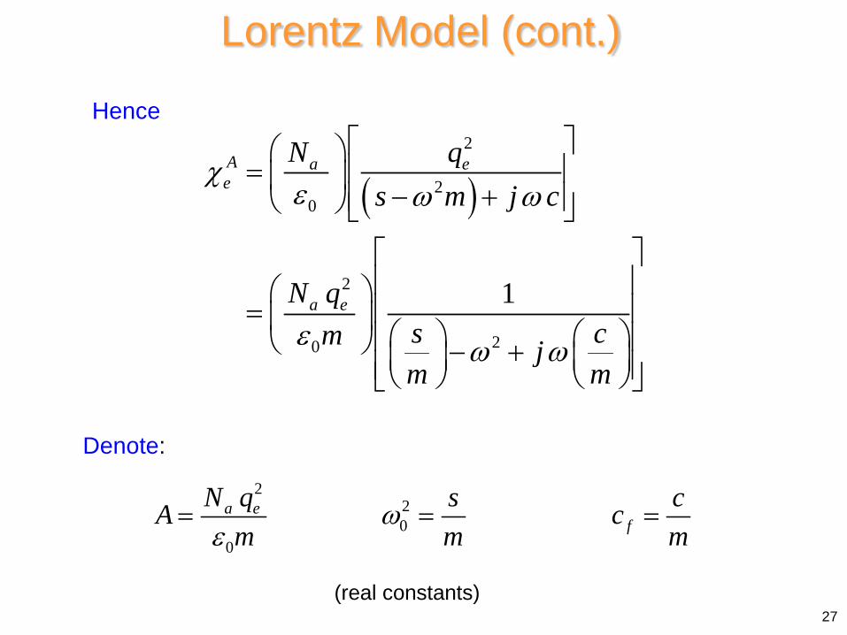
Denote:

( )2

20

2

20

1

A a ee

a e

N qs m j c

N qs cm jm m

χε ω ω

ε ω ω

=

− + = − +

220

0

a ef

N q s cA cm m m

ωε

= = =

Hence

(real constants)

Lorentz Model (cont.)

27

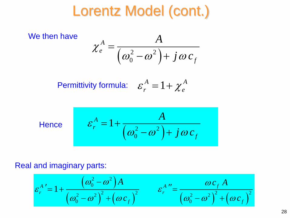
We then have

( )2 20

Ae

f

Aj c

χω ω ω

=− +

( )( ) ( ) ( ) ( )

2 20

2 22 22 2 2 20 0

1 fA Ar r

f f

A c A

c c

ω ω ωε ε

ω ω ω ω ω ω

−′ ′′= + =

− + − +

( )2 20

1Ar

f

Aj c

εω ω ω

= +− +

Permittivity formula: 1A Ar eε χ= +

Lorentz Model (cont.)

28

Hence

Real and imaginary parts:

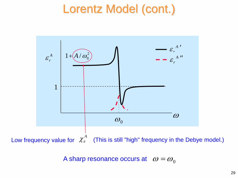
A sharp resonance occurs at 0ω ω=

Lorentz Model (cont.)

Low frequency value for Aeχ

Arε

0ω ω

1

Arε ′

Arε ′′

201 /A ω+

(This is still "high" frequency in the Debye model.)

29

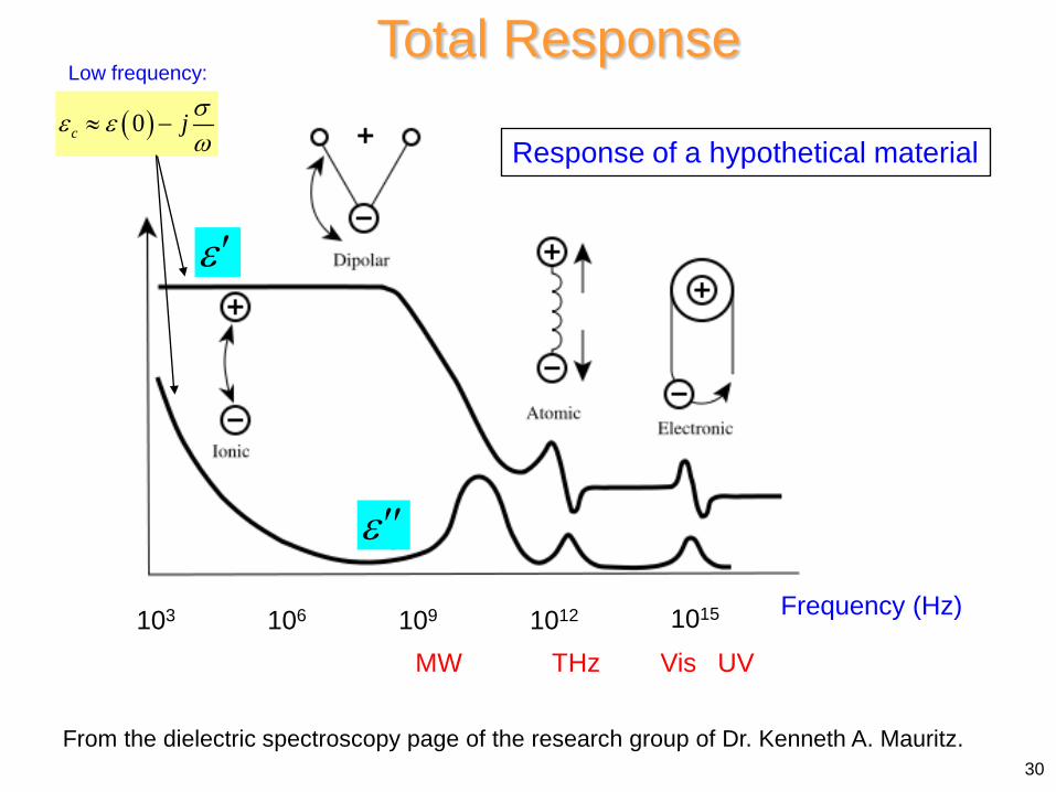
Total Response

From the dielectric spectroscopy page of the research group of Dr. Kenneth A. Mauritz.

Frequency (Hz)

Response of a hypothetical material

103 106 109 1012 1015

MW THz UV Vis

ε ′

ε ′′

30

( )0c j σε εω

≈ −

Low frequency:

Atmospheric Attenuation

60 GHz

90 GHz

31

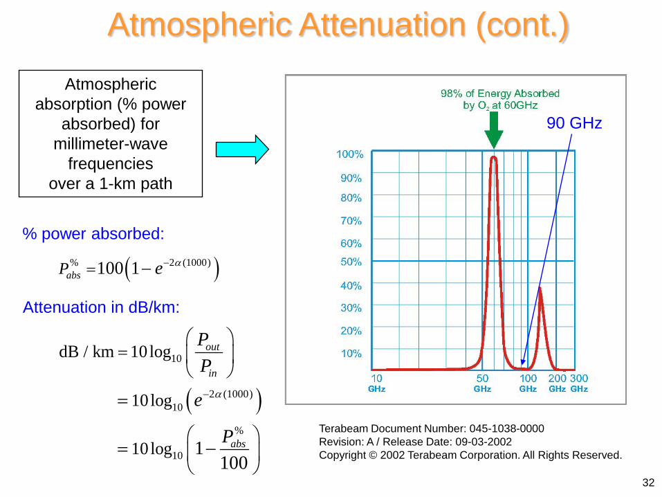
Atmospheric Attenuation (cont.) Atmospheric

absorption (% power absorbed) for

millimeter-wave frequencies

over a 1-km path

( )% 2 (1000)100 1absP e α−= −

( )

10

2 (1000)10

%

10

dB / km 10log

10log

10log 1100

out

in

abs

PP

e

P

α−

=

=

= −

Terabeam Document Number: 045-1038-0000 Revision: A / Release Date: 09-03-2002 Copyright © 2002 Terabeam Corporation. All Rights Reserved.

Attenuation in dB/km:

32

90 GHz

% power absorbed:

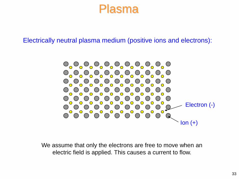
Plasma

Electrically neutral plasma medium (positive ions and electrons):

Ion (+)

Electron (-)

We assume that only the electrons are free to move when an electric field is applied. This causes a current to flow.

33

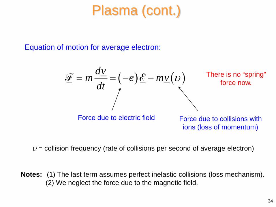
Plasma (cont.)

Equation of motion for average electron:

( ) ( )dvm e mvdt

υ= = − −F E

υ = collision frequency (rate of collisions per second of average electron)

Notes: (1) The last term assumes perfect inelastic collisions (loss mechanism). (2) We neglect the force due to the magnetic field.

Force due to electric field Force due to collisions with ions (loss of momentum)

There is no “spring” force now.

34

Plasma (cont.)

Sinusoidal steady state:

( ) ( )m j v e E mvω υ= − −

( )( )

ev E

m jω υ−

=+

Current: ( )

( )ve

ve

eJ v E

m jρ

ρω υ

−= = +

35

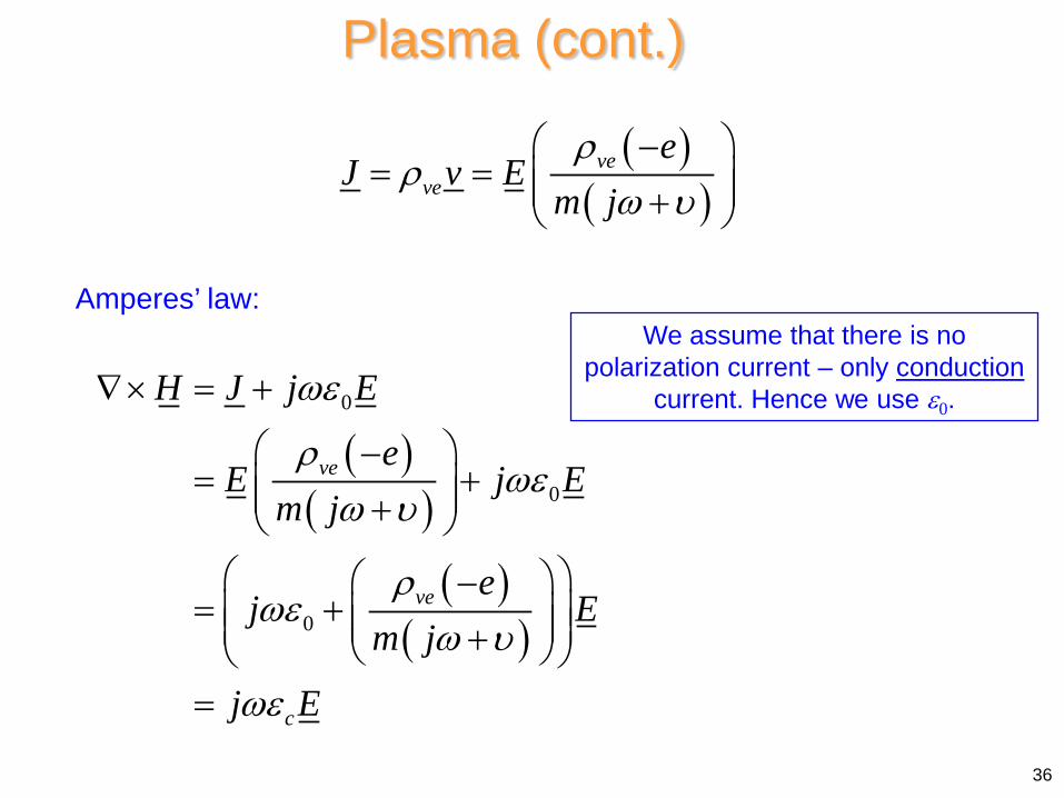
Plasma (cont.)

Amperes’ law:

( )( )

( )( )

0

0

0

ve

ve

c

H J j E

eE j E

m j

ej E

m j

j E

ωε

ρωε

ω υ

ρωε

ω υ

ωε

∇× = +

−= + +

−= + + =

( )( )

veve

eJ v E

m jρ

ρω υ

−= = +

We assume that there is no polarization current – only conduction

current. Hence we use ε0.

36

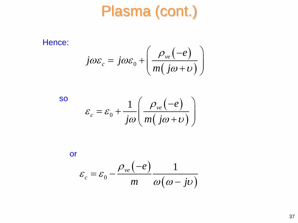
Plasma (cont.)

Hence: ( )

( )0ve

c

ej j

m jρ

ωε ωεω υ

−= + +

so ( )( )0

1 vec

ej m j

ρε ε

ω ω υ −

= + +

or ( )

( )01ve

c

em j

ρε ε

ω ω υ−

= −−

37

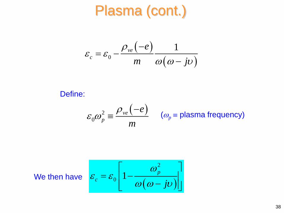
Plasma (cont.)

Define:

( )20

vep

em

ρε ω

−≡

( )

2

0 1 pc j

ωε ε

ω ω υ

= − −

(ωp ≡ plasma frequency)

We then have

( )( )0

1vec

em j

ρε ε

ω ω υ−

= −−

38

Plasma (cont.)

Lossless plasma:

2

0 1 pc

ωε ε

ω

= −

0υ =

(Drude equation)

0

0

: 0, ( )

: 0, ( )p c c c

p c c c

k

k j

ω ω ε ε ω µ ε β

ω ω ε ε ω µ ε α

> = > = =

< = − < = = −

propagation

attenuation

Plane wave in lossless plasma:

39

Plasma (cont.)

Measured complex relative permittivity of silver at optical frequencies

Rel

ativ

e pe

rmitt

ivity

The Drude model is an approximate model for how metals behave at optical frequencies.

40

“Plasmonic behavior”

149.23 10 [Hz]pf = ×

Visible

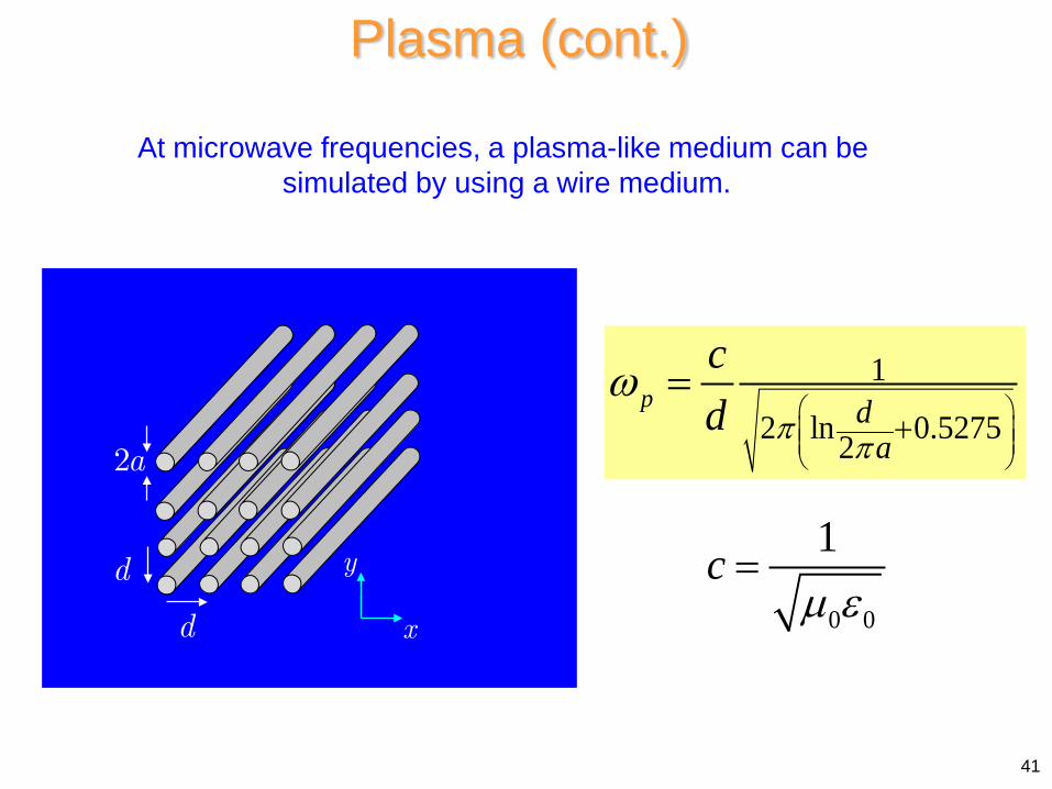
Plasma (cont.)

At microwave frequencies, a plasma-like medium can be simulated by using a wire medium.

d

d

2a

y

x

1

2 ln 0.52752p d

a

cd π π

ω

+=

0 0

1cµ ε

=

41

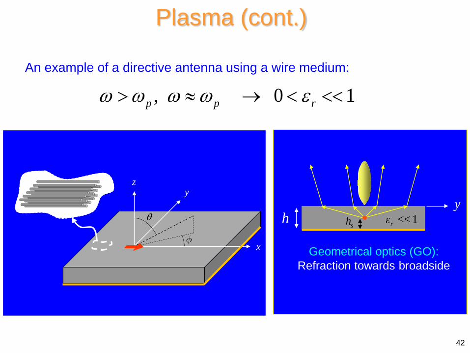
Plasma (cont.)

An example of a directive antenna using a wire medium:

Geometrical optics (GO): Refraction towards broadside

y<< 1rεh

sh

θ

x

yzx

, 0 1p p rω ω ω ω ε> ≈ → < <<

42