ece 320h1f fields and waves problem set 1 - skule
TRANSCRIPT

ECE 320H1F – FIELDS AND WAVES
PROBLEM SET 1
Purpose: To review the use of phasor quantities, calculus of sinusoidal functions, practice transmission-line concepts. Textbook Coverage: Ulaby 1-1 to 1-7, 2-1 to 2-4. Problems from Ulaby: 1.28, 1.29, 2.1, 2.8. Note: Problems indicated with a * will be discussed during the tutorials.
A. PROBLEMS ON PHASORS
1. Prove that for a sinusoidal function ),( tza where z is the space coordinate and t is the time coordinate, there exists a phasor !A(z) such that:
a) ∂∂ta(z, t) = ∂
∂tRe{ !A(z)e jωt} (1)
b) ∂∂ta(z, t) = Re{ jω !A(z)e jωt} (2)
2. Show that: ∂2
∂t2a(z, t) = Re{−ω 2 !A(z)e jωt}
3. * Prove that ifRe{ !A(z)e jωt} = Re{ !B(z)e jωt} , then !A(z) = !B(z) (hence, the operator
Re{} can be removed from phasors of the same frequency).
4. *Show that Re !A(z)e jωt{ }Re !B(z)e jωt{ }timeavg
=12Re !A(z) !B*(z){ } .
UNIVERSITY OF TORONTO FACULTY OF APPLIED SCIENCE AND ENGINEERING The Edward S. Rogers Sr. Department of Electrical and Computer Engineering
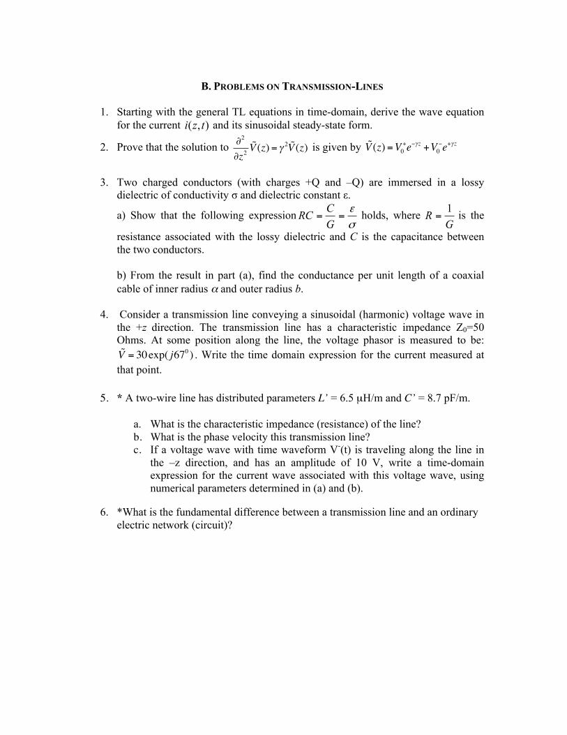
B. PROBLEMS ON TRANSMISSION-LINES
1. Starting with the general TL equations in time-domain, derive the wave equation
for the current ),( tzi and its sinusoidal steady-state form.
2. Prove that the solution to ∂2
∂z2!V (z) = γ 2 !V (z) is given by !V (z) =V0
+e−γz +V0−e+γz
3. Two charged conductors (with charges +Q and –Q) are immersed in a lossy
dielectric of conductivity σ and dielectric constant ε.
a) Show that the following expressionσε
==GCRC holds, where
GR 1= is the
resistance associated with the lossy dielectric and C is the capacitance between the two conductors.
b) From the result in part (a), find the conductance per unit length of a coaxial cable of inner radius α and outer radius b.
4. Consider a transmission line conveying a sinusoidal (harmonic) voltage wave in the +z direction. The transmission line has a characteristic impedance Z0=50 Ohms. At some position along the line, the voltage phasor is measured to be:!V = 30exp( j670 ) . Write the time domain expression for the current measured at
that point.
5. * A two-wire line has distributed parameters L’ = 6.5 µH/m and C’ = 8.7 pF/m.
a. What is the characteristic impedance (resistance) of the line? b. What is the phase velocity this transmission line? c. If a voltage wave with time waveform V-(t) is traveling along the line in
the –z direction, and has an amplitude of 10 V, write a time-domain expression for the current wave associated with this voltage wave, using numerical parameters determined in (a) and (b).
6. *What is the fundamental difference between a transmission line and an ordinary electric network (circuit)?
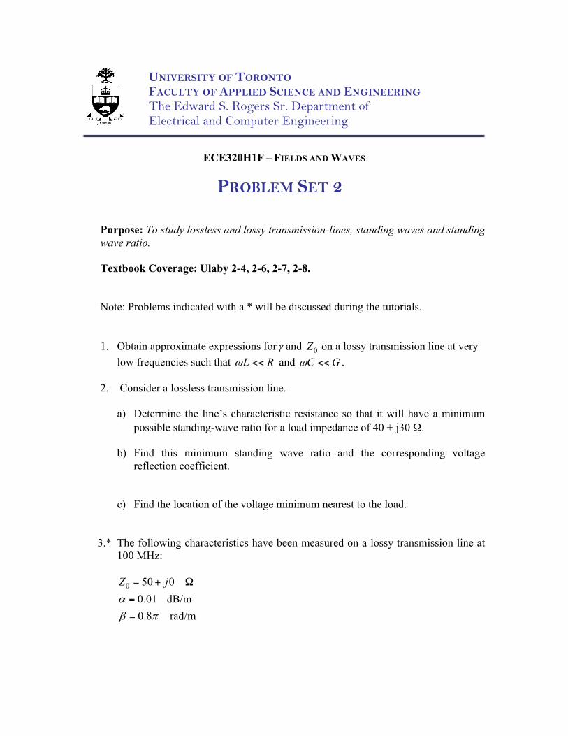
ECE320H1F – FIELDS AND WAVES
PROBLEM SET 2
Purpose: To study lossless and lossy transmission-lines, standing waves and standing wave ratio. Textbook Coverage: Ulaby 2-4, 2-6, 2-7, 2-8. Note: Problems indicated with a * will be discussed during the tutorials.
1. Obtain approximate expressions forγ and 0Z on a lossy transmission line at very low frequencies such that L R<<ω and C G<<ω .
2. Consider a lossless transmission line.
a) Determine the line’s characteristic resistance so that it will have a minimum
possible standing-wave ratio for a load impedance of 40 + j30 Ω. b) Find this minimum standing wave ratio and the corresponding voltage
reflection coefficient.
c) Find the location of the voltage minimum nearest to the load.
3.* The following characteristics have been measured on a lossy transmission line at 100 MHz:
0 50 00.01 dB/m0.8 rad/m
Z j= + Ω
=
=
α
β π
UNIVERSITY OF TORONTO FACULTY OF APPLIED SCIENCE AND ENGINEERING The Edward S. Rogers Sr. Department of Electrical and Computer Engineering
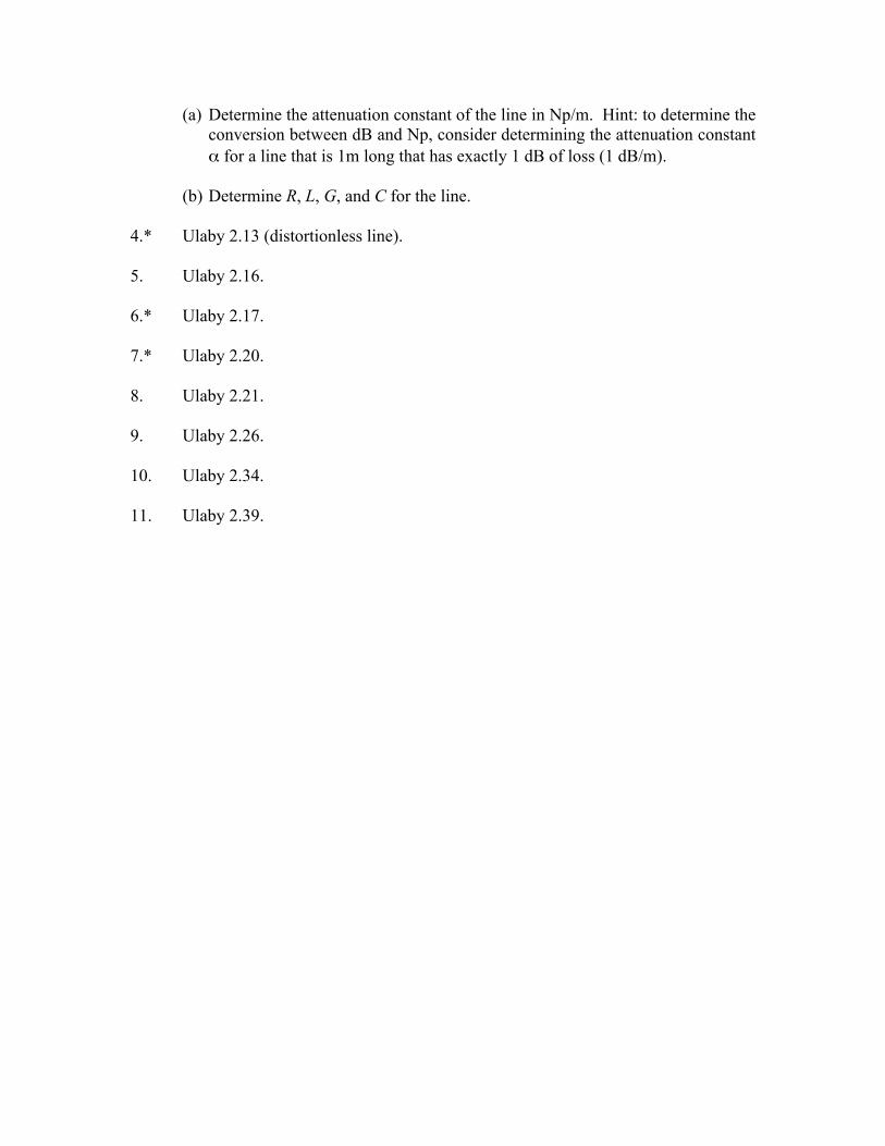
(a) Determine the attenuation constant of the line in Np/m. Hint: to determine the conversion between dB and Np, consider determining the attenuation constant α for a line that is 1m long that has exactly 1 dB of loss (1 dB/m).
(b) Determine R, L, G, and C for the line. 4.* Ulaby 2.13 (distortionless line). 5. Ulaby 2.16. 6.* Ulaby 2.17. 7.* Ulaby 2.20. 8. Ulaby 2.21. 9. Ulaby 2.26. 10. Ulaby 2.34. 11. Ulaby 2.39.
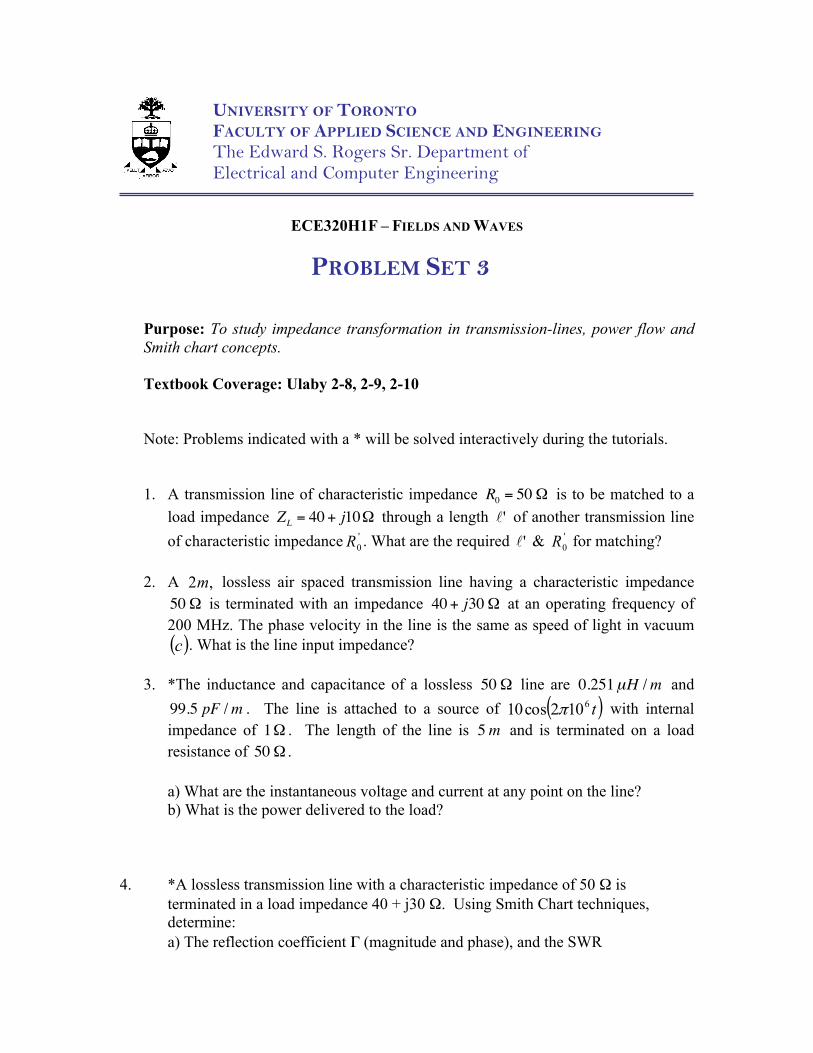
ECE320H1F – FIELDS AND WAVES
PROBLEM SET 3
Purpose: To study impedance transformation in transmission-lines, power flow and Smith chart concepts. Textbook Coverage: Ulaby 2-8, 2-9, 2-10 Note: Problems indicated with a * will be solved interactively during the tutorials.
1. A transmission line of characteristic impedance R0 = 50Ω is to be matched to a load impedance ZL = 40+ j10Ω through a length 'ℓ of another transmission line of characteristic impedance '
0R . What are the required 'ℓ & '0R for matching?
2. A ,2m lossless air spaced transmission line having a characteristic impedance
50Ω is terminated with an impedance 40+ j30Ω at an operating frequency of 200 MHz. The phase velocity in the line is the same as speed of light in vacuum ( )c . What is the line input impedance?
3. *The inductance and capacitance of a lossless 50Ω line are 0.251µH /m and
99.5 pF /m . The line is attached to a source of ( )t6102cos10 π with internal impedance of 1Ω . The length of the line is 5m and is terminated on a load resistance of 50Ω .
a) What are the instantaneous voltage and current at any point on the line? b) What is the power delivered to the load?
4. *A lossless transmission line with a characteristic impedance of 50 Ω is
terminated in a load impedance 40 + j30 Ω. Using Smith Chart techniques, determine:
a) The reflection coefficient Γ (magnitude and phase), and the SWR
UNIVERSITY OF TORONTO FACULTY OF APPLIED SCIENCE AND ENGINEERING The Edward S. Rogers Sr. Department of Electrical and Computer Engineering

b) The input admittance seen looking into the line if it is 0.2λ long. c) The length of line needed to make the input impedance look real (one solution
is sufficient), and the associated resistance value. 5. Ulaby 2.42, 2.43, 2.44*, 2.47*, 2.49*, 2.52, 2.53, 2.55, 2.59

ECE320H1F – FIELDS AND WAVES
PROBLEM SET 4
Purpose: Practice impedance matching via Smith chart, study of transients on transmission lines. Textbook Coverage: Ulaby 2-10, 2-11, 2-12. Note: Problems indicated with a * will be solved interactively during the tutorials.
Ulaby 2.63, 2.66*, 2.68, 2.72, 2.74*, 2,77*, 2.80*
[ECE357, Term test 1, Spring 2007] An unknown impedance ZL is to be measured at 500 MHz, via a transmission-line of characteristic impedance Z0 =50 Ohms and up=c (where c=3x10⁸ m/sec is the speed of light). With the load ZL in place, the Standing-Wave Ratio is measured to be S=3.2, with a voltage minimum occurring at d=z’ away from the load. Replacing ZL with a short-circuit, the first voltage null away from the short-circuit is observed at cm2.8zz −ʹ=ʹ́ . Determine ZL. You can use the Smith chart for this question. [ECE357 Term test 2, Spring 2007] Determine the parameters of the matching network shown in the figure below, to transform a load impedance ZL=150+j50 Ohms into an input impedance Zin=20-j100 Ohms. The transmission-lines of the network have a characteristic impedance Z0 =50 Ohms. Is it possible to perform this matching by connecting the open stub at A-A’?
UNIVERSITY OF TORONTO FACULTY OF APPLIED SCIENCE AND ENGINEERING The Edward S. Rogers Sr. Department of Electrical and Computer Engineering

[ECE357, Final exam, Spring 2007] On the Smith chart, show the normalized impedances zL that you can match to a 100 Ohm input impedance, using the matching network of Fig. 1b at 50 MHz. Extract the corresponding range of values for RL and XL. The transmission-line segment shown has a characteristic impedance of 50 Ohms,
sec/m103 8p ×=υ and the available length you can use is up to 1.5m.
d
L
Zin=20-j100
ZL=150+j50
A
A’

ECE320H1F – FIELDS AND WAVES
PROBLEM SET 5
Purpose: Review of vector calculus and Maxwell’s equations. Textbook Coverage: Ulaby Ch. 3, 4-1, 6-1, 6-2. Note: Problems indicated with a * will be solved interactively during the tutorials.
1. Ulaby 3.5*, 3.44*, 3.46, 3.56 2. Ulaby 6.1*, 6.2*, 6.3, 6.5*
UNIVERSITY OF TORONTO FACULTY OF APPLIED SCIENCE AND ENGINEERING The Edward S. Rogers Sr. Department of Electrical and Computer Engineering

ECE320H1F – FIELDS AND WAVES
PROBLEM SET 6
Purpose: Review of Maxwell’s equations (note: this material has been covered in ECE221; review of the relevant parts of ECE221 is highly recommended). Textbook Coverage: Ulaby Ch. 6-3 to 6-10 (inclusive) Note: Problems indicated with a * will be solved interactively during the tutorials.
1. Ulaby 6-10, 6-12*, 6-14, 6-15, 6-16*, 6-17, 6-18*, 6-22*
UNIVERSITY OF TORONTO FACULTY OF APPLIED SCIENCE AND ENGINEERING The Edward S. Rogers Sr. Department of Electrical and Computer Engineering
ECE320H1F – FIELDS AND WAVES
PROBLEM SET 7
Purpose: Study of Maxwell’s equations for time-harmonic fields and the use of phasors. Textbook Coverage: Ulaby Ch. 6-3 to 6-10 (inclusive) and 6-11 from equation 6.86 onwards (disregard “potentials”). Note: Problems indicated with a * will be solved during the tutorials.
Ulaby 6-23*, 6-24*, 6-25, 6-26, 6-28*, 6-29*.
UNIVERSITY OF TORONTO FACULTY OF APPLIED SCIENCE AND ENGINEERING The Edward S. Rogers Sr. Department of Electrical and Computer Engineering

ECE320H1F – FIELDS AND WAVES
PROBLEM SET 8
Topics: Plane-wave propagation, polarization Reading: Chapter 7: 7-1,7-2,7-3 Ulaby 7.1*, 7.3*, 7.4, 7.8, 7.9, 7.10, 7.11*, 7.12, 7.13*, 7.15*
UNIVERSITY OF TORONTO FACULTY OF APPLIED SCIENCE AND ENGINEERING The Edward S. Rogers Sr. Department of Electrical and Computer Engineering
ECE320H1F – FIELDS AND WAVES
PROBLEM SET 9
Topics: Plane-Wave Propagation, Propagation in lossy media, electromagnetic power Reading: Chapter 7: 7-4,7-5, 7-6 Ulaby 7.18, 7.19, 7.21*, 7.25, 7.27*, 7.29*, 7.31*, 7.33*, 7.35*, 7.39*
UNIVERSITY OF TORONTO FACULTY OF APPLIED SCIENCE AND ENGINEERING The Edward S. Rogers Sr. Department of Electrical and Computer Engineering

ECE 320H1F – FIELDS AND WAVES
PROBLEM SET 10
Purpose: Understand wave reflection and transmission. Emphasis on normal incidence on a medium, nature of oblique plane waves, oblique incidence on a dielectric medium, transmission-line analogy. Textbook Coverage: Ulaby 8-1,8-2, 8-3,8-4 Problems from Ulaby: 8.1, 8.2*, 8.4*, 8.9, 8.10, 8.14*, 8.17*, 8.27*
UNIVERSITY OF TORONTO FACULTY OF APPLIED SCIENCE AND ENGINEERING The Edward S. Rogers Sr. Department of Electrical and Computer Engineering

ECE 320H1F – FIELDS AND WAVES
PROBLEM SET 11
Purpose: Understand wave reflection and transmission. TM and TE oblique incidence on a dielectric medium, transmission-line analogy, Brewster angle, total-internal reflection. Textbook Coverage: Ulaby 8-1,8-2, 8-3,8-4, 8-5 Problems from Ulaby: 8.23,8.29*,8.32*,8.35,8.36*,8.37
UNIVERSITY OF TORONTO FACULTY OF APPLIED SCIENCE AND ENGINEERING The Edward S. Rogers Sr. Department of Electrical and Computer Engineering